Wavefront construction using waverays

Stanford Exploration Project, Report 80, May 15, 2001, pages 1–102

Wavefront construction using waverays

Hector Urdaneta1

ABSTRACT

A method for computing first arrival traveltimes and amplitudes in a general two-dimensional (2-D) velocity model is presented. The method is the result of merging tworecently published ray tracing methods. The product is a very robust algorithm that is ableto produce broadband wave phenomena, such as dispersion and wavelength dependentscattering. Its ability to produce broadband wave phenomena, is achieved by performinga wavelength-dependent smoothing of the velocity model across wavefronts. In the limitof high frequency, the method reduces to geometrical ray theory. The method is able toilluminate areas of large geometrical spreading where conventional ray tracing methodsmay give no arrivals. The method is tested on synthetic complex velocity models.

INTRODUCTION

Traditionally traveltime and amplitude calculations have been performed by ray tracing. Dif-ferent ray tracing algorithms exist that are well known and well documented. They includeJulian and Gubbins’ (1977) ray bending, Dines and Lytle’s (1979) shooting rays andCer-vený’s (1987) paraxial extrapolation. More recently, several new methods have appeared andare enjoying an increasing popularity. They include Vidale (1990), Podvin and Lecomte (1991),van Trier and Symes (1991) finite differences and Moser’s (1991) shortest path rays. This pa-per presents a review of two new ray tracing methods and explores some of the possibilitiesproduced by their fusion. The first method is Lomax’s (1994) waveray method for approxi-mating broadband wave propagation through complex velocity structures. The second methodwas developed at the NORSAR institute in Norway by Vinje, Iversen and Gjøystdal (1993). Aswill be shown later, both methods have their own advantages and drawbacks, but when theyare fused, they interfere positively. The combined product produces a very robust method,which approximates broadband wave phenomena in complex velocity models. The first twoparts of this paper describe the basic characteristics of each method and their implementations.The paper also reviews some of the work done in the last two references listed above. In thelast part, I discuss the combined method. Implementation issues and synthetic examples areshown.

1email: not available

1

2 Urdaneta SEP–80

LOMAX’S WAVERAYS

Two basic ideas characterize Lomax’s method: (1) it does a wavelength-dependent velocitysmoothing and (2) it uses Huygen’s principle to track the motion of narrow-band wavefrontsat a number of center frequencies. Narrow-band wavefronts are defined as surfaces (lines in2-D) of constant phase or traveltime in a narrow-band “wavefield”. As these narrow-bandwavefronts propagate with time they define a wavepath, which is frequency dependent. Thewavelength-dependent smoothing of the velocity is done by averaging with a Gaussian weight-ing curve. The smoothing is done along the wavefronts. The final result; i.e, the broadbandwavefield, is constructed by summing the results of independent narrow-band wavefields atmany center frequencies. Three important advantages of using Lomax’s waveray over con-ventional ray tracing methods are:

• It increases the stability of wavepaths compared to the paths produced by high frequencymethods, due to the wavelength-dependent smoothing.

• It provides waverays with a sensitivity that produces frequency dependent scattering asa function of the ratio of wavelength to the characteristic size of the scattering region.Figure 3 illustrates this point.

• It is capable of handling large to small inhomogeneity sizes, since in the former caseit is similar to ray theory and in the latter it responds to a smooth, averaged velocitystructure.

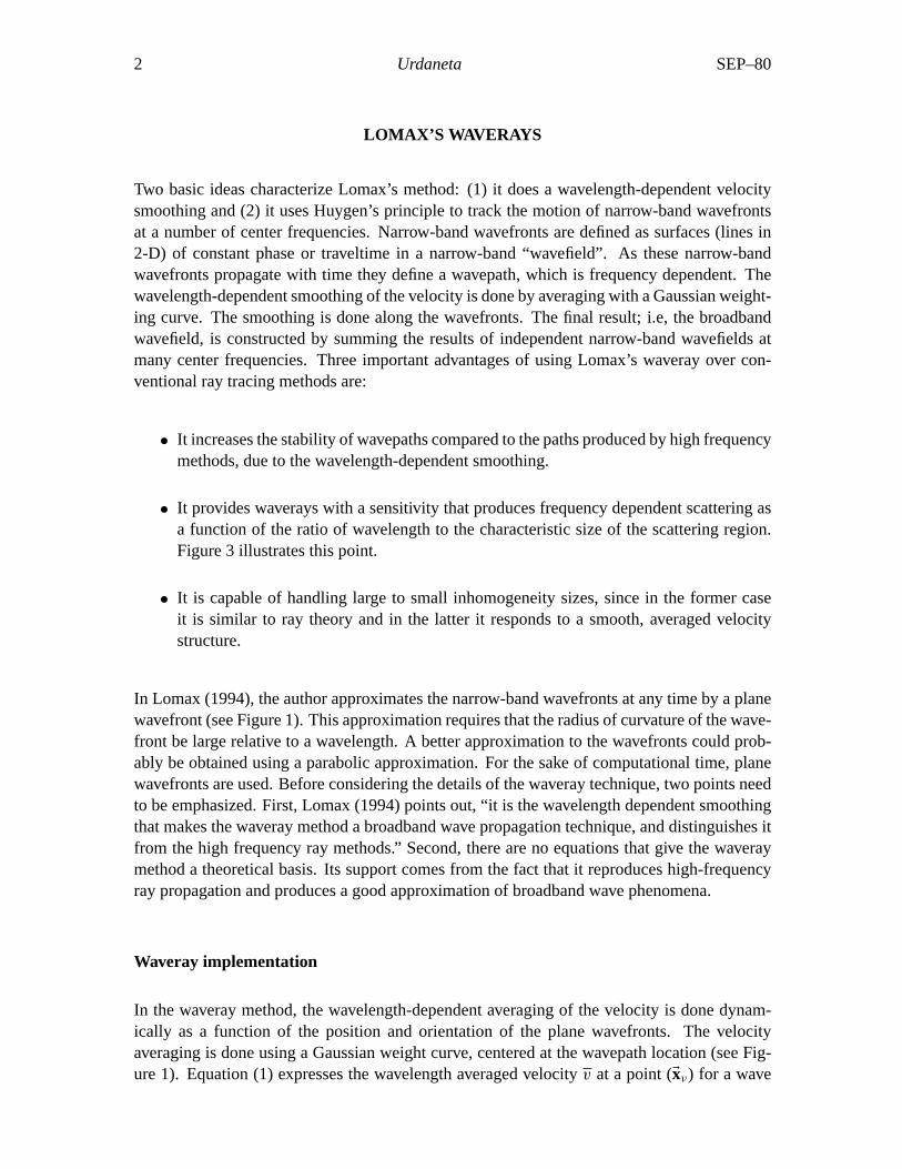
In Lomax (1994), the author approximates the narrow-band wavefronts at any time by a planewavefront (see Figure 1). This approximation requires that the radius of curvature of the wave-front be large relative to a wavelength. A better approximation to the wavefronts could prob-ably be obtained using a parabolic approximation. For the sake of computational time, planewavefronts are used. Before considering the details of the waveray technique, two points needto be emphasized. First, Lomax (1994) points out, “it is the wavelength dependent smoothingthat makes the waveray method a broadband wave propagation technique, and distinguishes itfrom the high frequency ray methods.” Second, there are no equations that give the waveraymethod a theoretical basis. Its support comes from the fact that it reproduces high-frequencyray propagation and produces a good approximation of broadband wave phenomena.

Waveray implementation

In the waveray method, the wavelength-dependent averaging of the velocity is done dynam-ically as a function of the position and orientation of the plane wavefronts. The velocityaveraging is done using a Gaussian weight curve, centered at the wavepath location (see Fig-ure 1). Equation (1) expresses the wavelength averaged velocityv at a point (Exν) for a wave

SEP–80 Waverays and wavefronts 3

Figure 1: Waveray wavepath andwavelength-dependent velocitysmoothing at pointExν Adapted fromLomax (1994). hector-lomax1[NR]

wavepath

instantaneouswavefront wavelength−dependent

weighting function

νXs

n

periodT (Lomax, 1994),

v (Exν ,T) =

∫∞

−∞

ω(γ ) c[Ex(γ ,T)] dγ∫∞

−∞

ω(γ ) dγ

(1)

whereγ is the arc length along the wavefront away fromExν expressed in wavelengths.c(Ex) isthe velocity at pointEx andω(γ ) is the Gaussian weight curve:

ω(γ ) = e−4ln2· (γ /α)2 (2)

whereα specifies the half width of the Gaussian bell in wavelengths. (Ex(γ ,T)) is the positionalong the instantaneous straight wavefront given by the recursive relation (Lomax, 1994):

Ex(γ ,T) = Exν +T2π

∫ γ

0c[Ex(γ ′,T)] n(T) dγ ′ (3)

wheren is the unit normal to the wavepath at pointExν . The discrete representation of equa-tion (1) is given by equation (4):

v (Exν ,T) =

N∑n=−N

ωn c[Exnν (T)]

N∑n=−N

ωn

(4)

where the integral has been replaced by a finite sum over 2N +1 control points. The positionof the control points along the wavefronts are given by equations (5) and (6).

Exν = Ex0ν (5)

4 Urdaneta SEP–80

Exnν =

Exn−1ν +

γmax

4π Nλ (Exn−1

ν ) n n = 1,2,. . . , N.

Exn+1ν −

γmax

4π Nλ (Exn+1

ν ) n n = −1,−2,. . . ,−N.

(6)

These two equations are the discrete version of equation (3), but, the dependence on the wave-length has been made explicit. Notice that the subscriptν of Exn

ν runs along the wavepath andthe superscriptn runs along the wavefront.γmax specifies the largest distance in wavelengthsalong the wavefront at which smoothing is applied. The discrete equivalent of the Gaussianweight function is:

ωn = e−4ln2· (γn/α)2 (7)

where the distanceγn along the wavefront in wavelengths is expressed as:

γn =nγmax

N(8)

The motion of the waverays along the direction of propagation is expressed by the followingequation:

Exν+1 = Exν +vν 1t s (9)

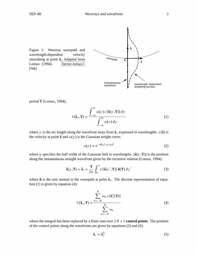
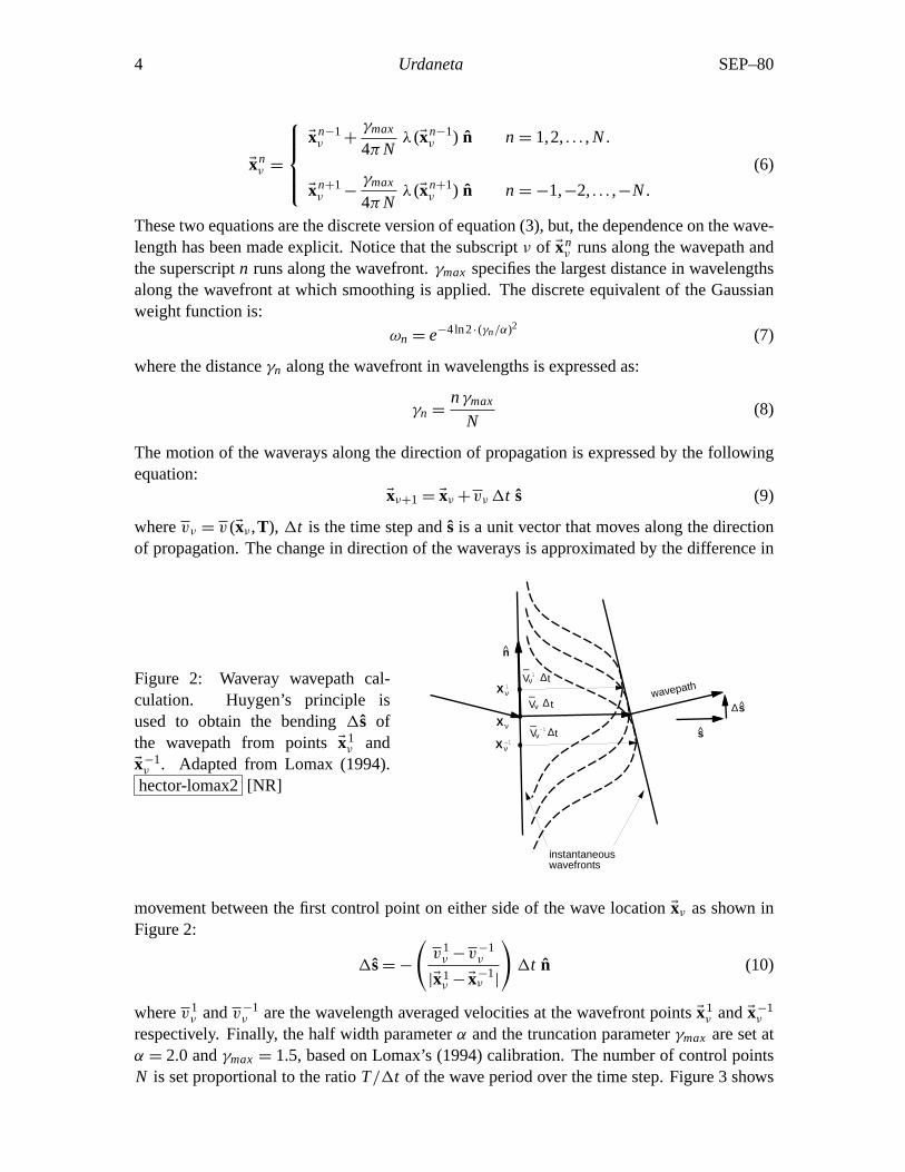
wherevν = v (Exν ,T), 1t is the time step ands is a unit vector that moves along the directionof propagation. The change in direction of the waverays is approximated by the difference in

Figure 2: Waveray wavepath cal-culation. Huygen’s principle isused to obtain the bending1s ofthe wavepath from pointsEx1

ν andEx−1ν . Adapted from Lomax (1994).hector-lomax2[NR]

V t

V twavepath

s

1X

X

−1X

∆

instantaneouswavefronts

s

n

_V t−1 ∆

_

_∆1

∆ν

ν

ν

ν

ν

ν

movement between the first control point on either side of the wave locationExν as shown inFigure 2:

1s= −

(v1

ν −v−1ν

|Ex1ν −Ex−1

ν |

)1t n (10)

wherev1ν andv−1

ν are the wavelength averaged velocities at the wavefront pointsEx1ν andEx−1

ν

respectively. Finally, the half width parameterα and the truncation parameterγmax are set atα = 2.0 andγmax = 1.5, based on Lomax’s (1994) calibration. The number of control pointsN is set proportional to the ratioT/1t of the wave period over the time step. Figure 3 shows


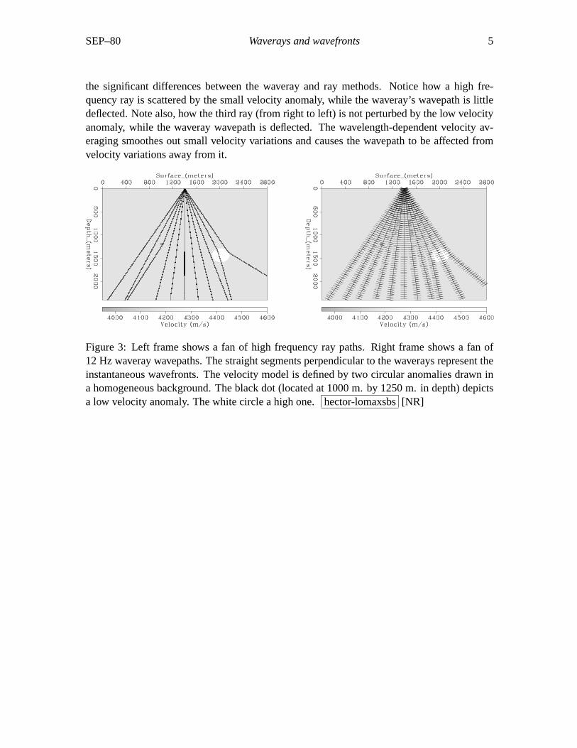
the significant differences between the waveray and ray methods. Notice how a high fre-quency ray is scattered by the small velocity anomaly, while the waveray’s wavepath is littledeflected. Note also, how the third ray (from right to left) is not perturbed by the low velocityanomaly, while the waveray wavepath is deflected. The wavelength-dependent velocity av-eraging smoothes out small velocity variations and causes the wavepath to be affected fromvelocity variations away from it.

Figure 3: Left frame shows a fan of high frequency ray paths. Right frame shows a fan of12 Hz waveray wavepaths. The straight segments perpendicular to the waverays represent theinstantaneous wavefronts. The velocity model is defined by two circular anomalies drawn ina homogeneous background. The black dot (located at 1000 m. by 1250 m. in depth) depictsa low velocity anomaly. The white circle a high one.hector-lomaxsbs[NR]

6 Urdaneta SEP–80

NORSAR WAVEFRONT CONSTRUCTION

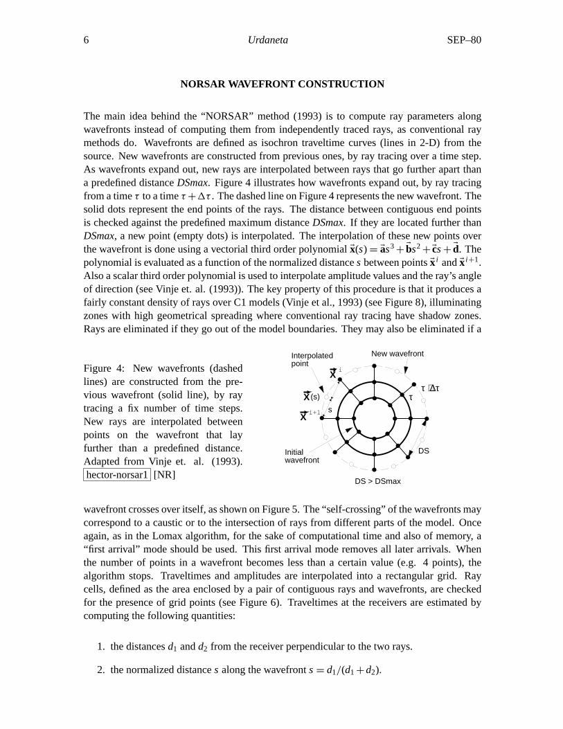
The main idea behind the “NORSAR” method (1993) is to compute ray parameters alongwavefronts instead of computing them from independently traced rays, as conventional raymethods do. Wavefronts are defined as isochron traveltime curves (lines in 2-D) from thesource. New wavefronts are constructed from previous ones, by ray tracing over a time step.As wavefronts expand out, new rays are interpolated between rays that go further apart thana predefined distanceDSmax. Figure 4 illustrates how wavefronts expand out, by ray tracingfrom a timeτ to a timeτ +1τ . The dashed line on Figure 4 represents the new wavefront. Thesolid dots represent the end points of the rays. The distance between contiguous end pointsis checked against the predefined maximum distanceDSmax. If they are located further thanDSmax, a new point (empty dots) is interpolated. The interpolation of these new points overthe wavefront is done using a vectorial third order polynomialEx(s) = Eas3

+ Ebs2+Ecs+ Ed. The

polynomial is evaluated as a function of the normalized distances between pointsEx i andEx i +1.Also a scalar third order polynomial is used to interpolate amplitude values and the ray’s angleof direction (see Vinje et. al. (1993)). The key property of this procedure is that it produces afairly constant density of rays over C1 models (Vinje et al., 1993) (see Figure 8), illuminatingzones with high geometrical spreading where conventional ray tracing have shadow zones.Rays are eliminated if they go out of the model boundaries. They may also be eliminated if a

Figure 4: New wavefronts (dashedlines) are constructed from the pre-vious wavefront (solid line), by raytracing a fix number of time steps.New rays are interpolated betweenpoints on the wavefront that layfurther than a predefined distance.Adapted from Vinje et. al. (1993).hector-norsar1[NR]

DS > DSmax

New wavefront

Initialwavefront

DS

Xi+1

Xi

Interpolatedpoint

X (s)

s

ττ + ∆τ

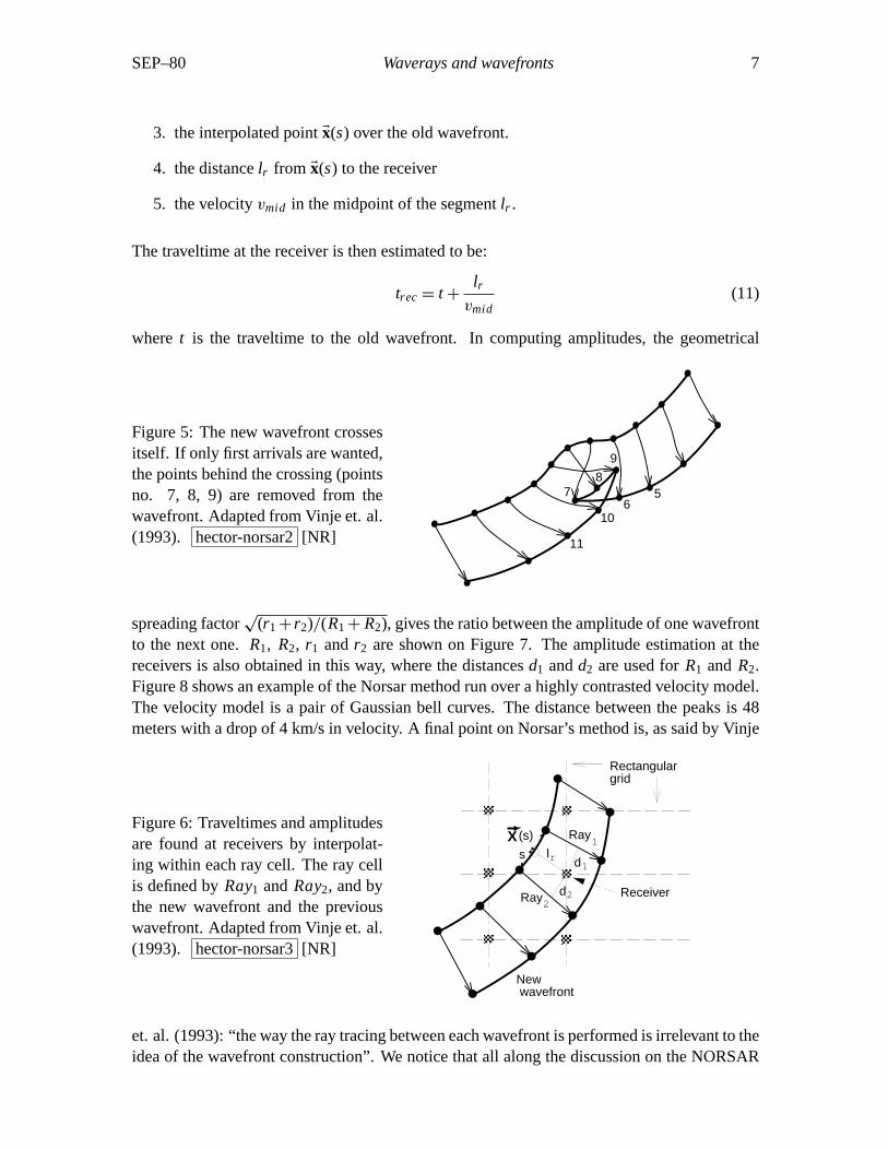
wavefront crosses over itself, as shown on Figure 5. The “self-crossing” of the wavefronts maycorrespond to a caustic or to the intersection of rays from different parts of the model. Onceagain, as in the Lomax algorithm, for the sake of computational time and also of memory, a“first arrival” mode should be used. This first arrival mode removes all later arrivals. Whenthe number of points in a wavefront becomes less than a certain value (e.g. 4 points), thealgorithm stops. Traveltimes and amplitudes are interpolated into a rectangular grid. Raycells, defined as the area enclosed by a pair of contiguous rays and wavefronts, are checkedfor the presence of grid points (see Figure 6). Traveltimes at the receivers are estimated bycomputing the following quantities:

1. the distancesd1 andd2 from the receiver perpendicular to the two rays.

2. the normalized distances along the wavefronts = d1/(d1 +d2).


3. the interpolated pointEx(s) over the old wavefront.

4. the distancelr from Ex(s) to the receiver

5. the velocityvmid in the midpoint of the segmentlr .

The traveltime at the receiver is then estimated to be:

trec = t +lr

vmid(11)

where t is the traveltime to the old wavefront. In computing amplitudes, the geometrical

Figure 5: The new wavefront crossesitself. If only first arrivals are wanted,the points behind the crossing (pointsno. 7, 8, 9) are removed from thewavefront. Adapted from Vinje et. al.(1993). hector-norsar2[NR]

56

8

10

11

9

7

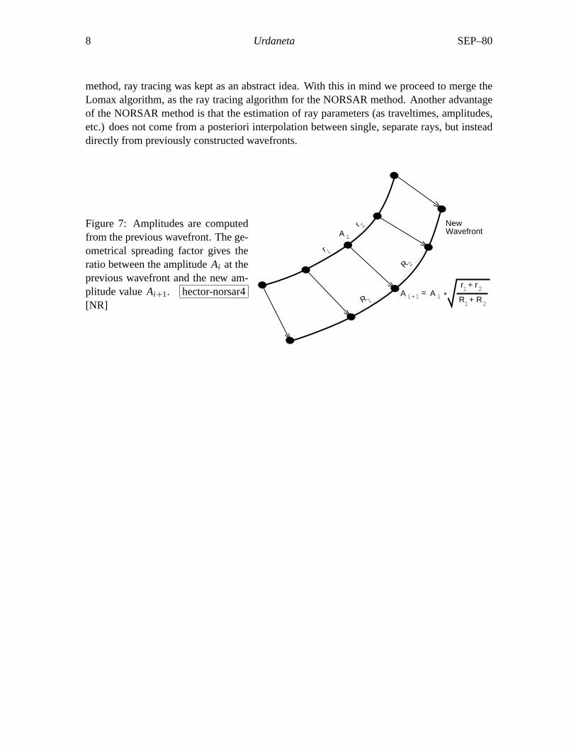
spreading factor√

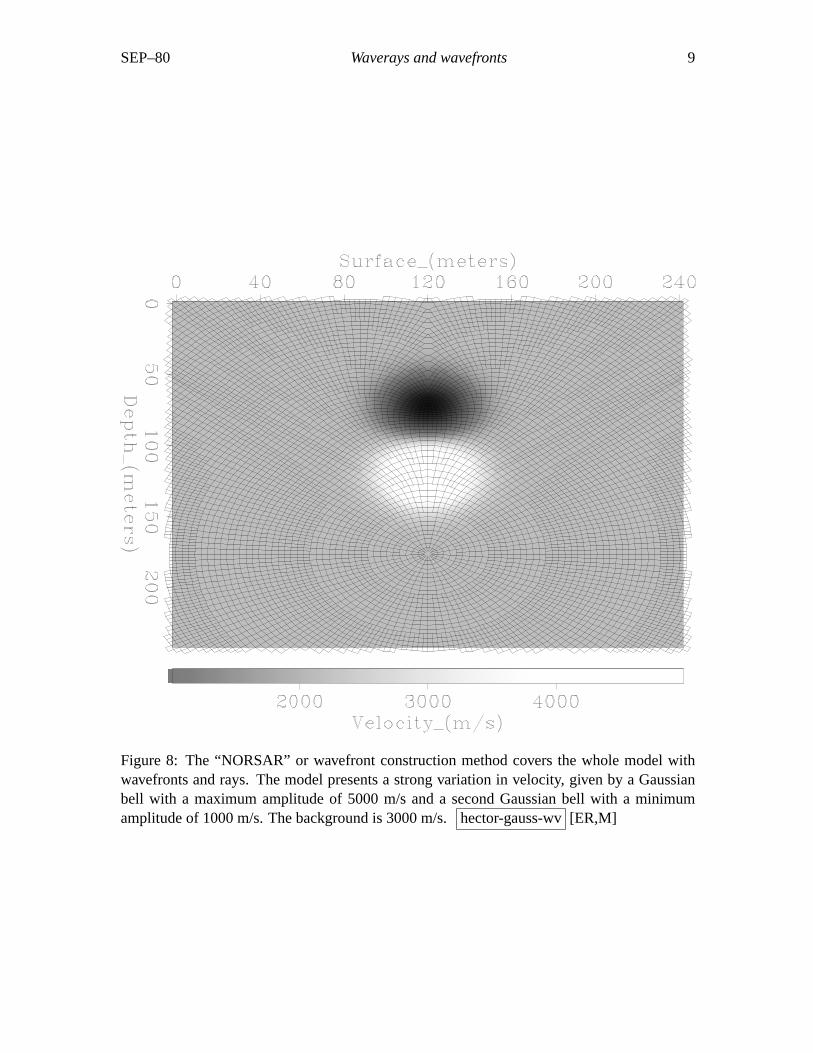
(r1 + r2)/(R1 + R2), gives the ratio between the amplitude of one wavefrontto the next one.R1, R2, r1 andr2 are shown on Figure 7. The amplitude estimation at thereceivers is also obtained in this way, where the distancesd1 andd2 are used forR1 and R2.Figure 8 shows an example of the Norsar method run over a highly contrasted velocity model.The velocity model is a pair of Gaussian bell curves. The distance between the peaks is 48meters with a drop of 4 km/s in velocity. A final point on Norsar’s method is, as said by Vinje

Figure 6: Traveltimes and amplitudesare found at receivers by interpolat-ing within each ray cell. The ray cellis defined byRay1 andRay2, and bythe new wavefront and the previouswavefront. Adapted from Vinje et. al.(1993). hector-norsar3[NR]

New wavefront

Receiver

d1

d2

lr1

Ray

2Ray

Rectangulargrid

s

(s)X

et. al. (1993): “the way the ray tracing between each wavefront is performed is irrelevant to theidea of the wavefront construction”. We notice that all along the discussion on the NORSAR

8 Urdaneta SEP–80

method, ray tracing was kept as an abstract idea. With this in mind we proceed to merge theLomax algorithm, as the ray tracing algorithm for the NORSAR method. Another advantageof the NORSAR method is that the estimation of ray parameters (as traveltimes, amplitudes,etc.) does not come from a posteriori interpolation between single, separate rays, but insteaddirectly from previously constructed wavefronts.

Figure 7: Amplitudes are computedfrom the previous wavefront. The ge-ometrical spreading factor gives theratio between the amplitudeAi at theprevious wavefront and the new am-plitude valueAi +1. hector-norsar4[NR]

NewWavefrontA i

A i+1 = A i * R + R1 2

r + r1 2

1r

r 2

1R

R 2


Figure 8: The “NORSAR” or wavefront construction method covers the whole model withwavefronts and rays. The model presents a strong variation in velocity, given by a Gaussianbell with a maximum amplitude of 5000 m/s and a second Gaussian bell with a minimumamplitude of 1000 m/s. The background is 3000 m/s.hector-gauss-wv[ER,M]

10 Urdaneta SEP–80

WAVERAYS AND WAVEFRONTS

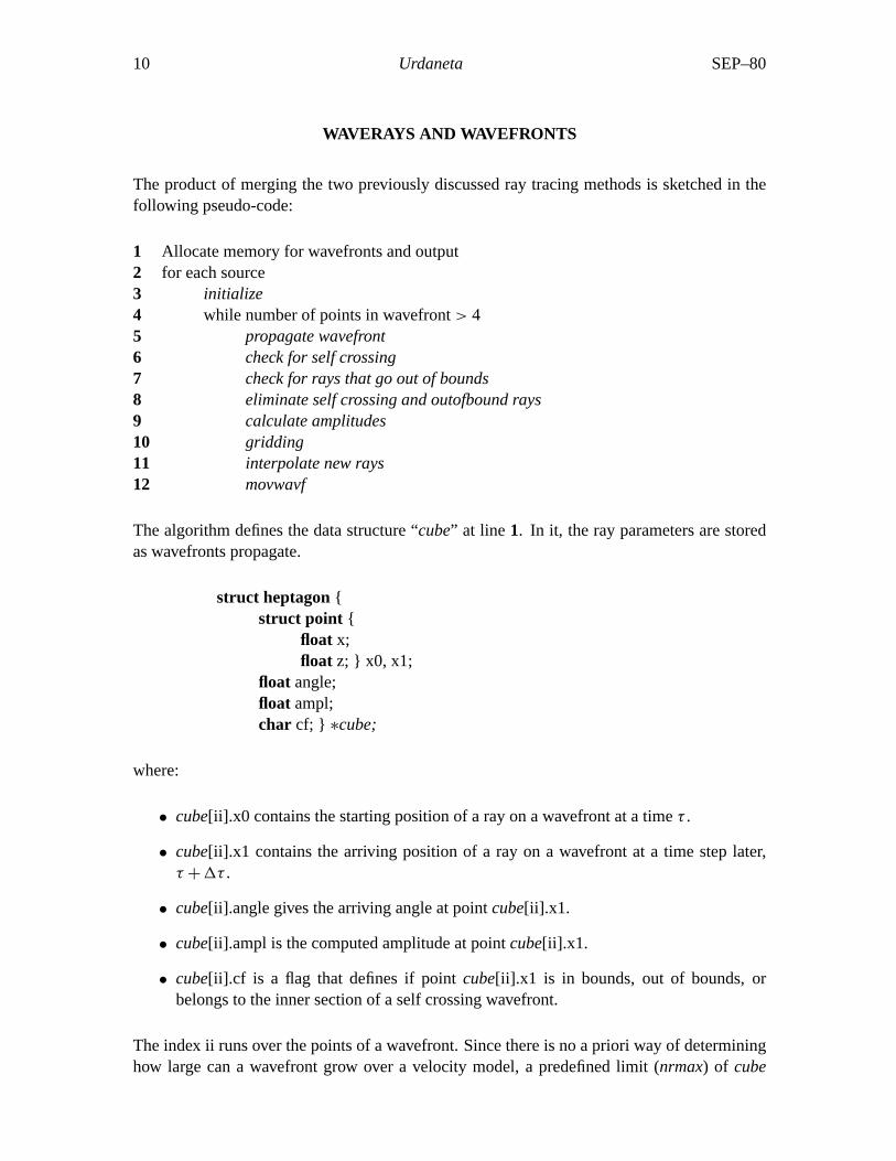
The product of merging the two previously discussed ray tracing methods is sketched in thefollowing pseudo-code:

1 Allocate memory for wavefronts and output2 for each source3 initialize4 while number of points in wavefront> 45 propagate wavefront6 check for self crossing7 check for rays that go out of bounds8 eliminate self crossing and outofbound rays9 calculate amplitudes10 gridding11 interpolate new rays12 movwavf

The algorithm defines the data structure “cube” at line 1. In it, the ray parameters are storedas wavefronts propagate.

struct heptagon{struct point {

float x;float z; } x0, x1;

float angle;float ampl;char cf; } ∗cube;

where:

• cube[ii].x0 contains the starting position of a ray on a wavefront at a timeτ .

• cube[ii].x1 contains the arriving position of a ray on a wavefront at a time step later,τ +1τ .

• cube[ii].angle gives the arriving angle at pointcube[ii].x1.

• cube[ii].ampl is the computed amplitude at pointcube[ii].x1.

• cube[ii].cf is a flag that defines if pointcube[ii].x1 is in bounds, out of bounds, orbelongs to the inner section of a self crossing wavefront.

The index ii runs over the points of a wavefront. Since there is no a priori way of determininghow large can a wavefront grow over a velocity model, a predefined limit (nrmax) of cube


elements is established at the beginning of the algorithm, which defines the total memoryallocated forcube. In other words,nrmaxis the maximum number of points that a wavefrontcan have. If the wavefront grows bigger thannrmaxpoints the algorithm is stopped and anerror message is produce indicating that a bigger value fornrmaxshould be used. This integerdepends directly on the maximum allowed separationDSmaxbetween two contiguous pointsin the wavefront. For the examples shown on Figure 9 through 12, the program ran with avalue ofnrmax=1300. DSmaxwas set to 21 meters for those examples. In the case that thealgorithm is run in a “all arrivals” mode, which could be done by eliminating line6 out of thealgorithm, the number of crossing points on a wavefront could become considerably large. Asthe wavefronts crosses and crosses many times over itself, for a velocity model with strongvariations (as for example the Marmousi model), the number of crossing points can easilyreach the 6 digits figure. This translates directly into a bigger need of computer resources, inuse of memory and time. Subroutineinitialize defines the initial wavefront. It assigns an initialamplitude and take-off angle to the points on the initial wavefront. Thepropagate wavefrontsubroutine ray traces using Lomax’s waverays. The waverays are traced starting atcube[ii].x0with a take-off anglecube[ii].angle during one time step at a certain frequency. The time stepand the frequency are user predefined. Subroutine on line6 checks for self crossed wavefrontsand flags the points that belong to the inner crossed section of the wavefront. Line7 checksfor points that fall out of boundaries, raising a flag. Notice from Figure 8 that the rays crossover the boundaries of the model. This is done in order to obtain arrivals at the receiversthat lie on the boundaries. Subroutine at line8 eliminates the points on a wavefront that areflagged for laying out of bounds or belong to self crossed wavefronts. Subroutines on lines9, 10 and11 are implemented as previously explained for the NORSAR method on Figures7, 6 and 4 respectively. On line11 the number of rays that may be interpolated betweenany two contiguous rays, is given by the number of times the distance between the two raysis bigger than the maximum allowed distanceDSmax. Subroutinegridding is a very timeconsuming, due to the irregular distribution of the data in the model. First, the subroutinechecks for receivers inside the ray cells of two contiguous wavefronts. If a receiver is found,the ray parameters are interpolated to it. Subroutinemovwavfprepares the structurecubefor anew wavefront to be propagated. It takes as the new starting point the previous arriving point(cube[ii].x0 = cube[ii].x1).

Travel-times and amplitudes in the Marmousi model

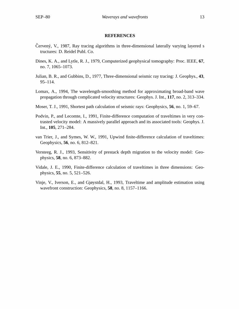
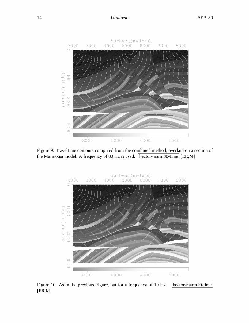
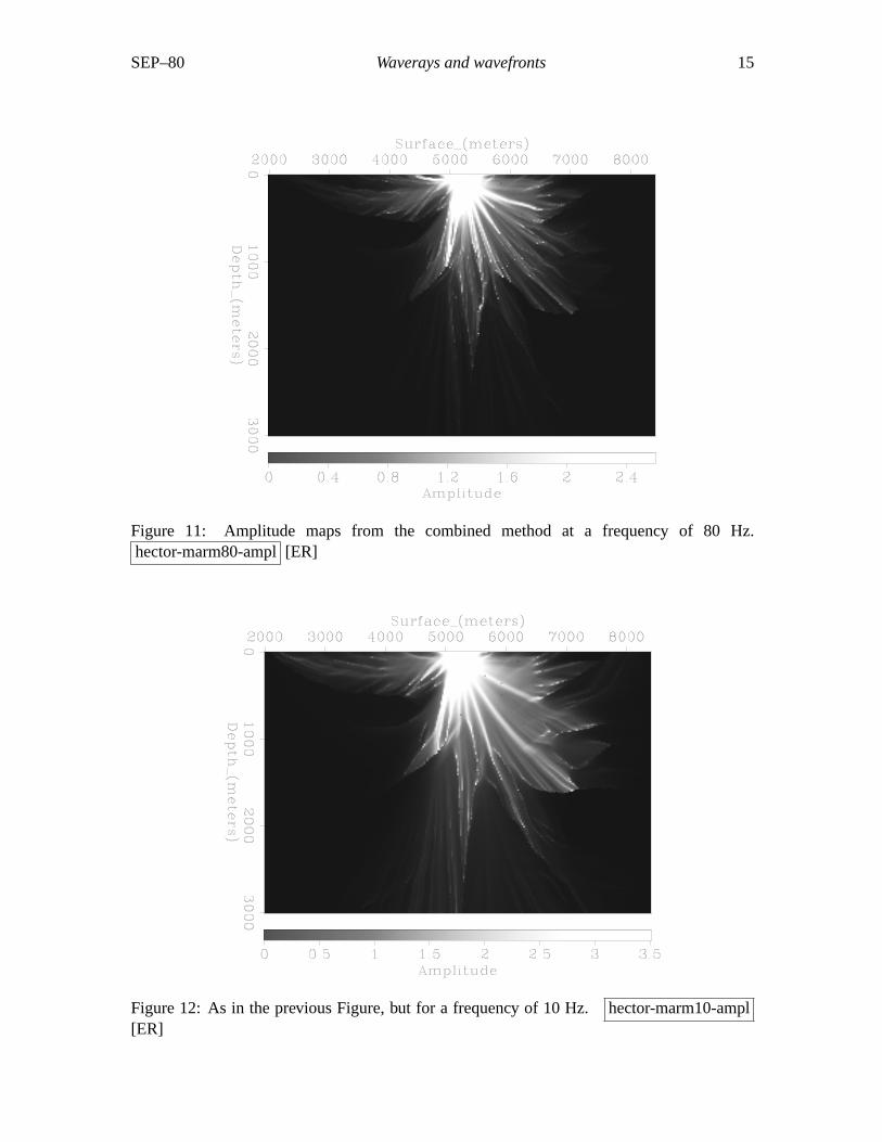
Figures 9 to 12 display the results of a simulation that used the combined method. The under-lying subsurface structure is the Marmousi model (Versteeg, 1993). A source was put at thesurface, 5200 meters away from the left edge of the model, and the wavefronts were propa-gated until they crossed the boundaries of the model. Figure 9 shows the first-arrival traveltimecontours calculated at a frequency of 80 Hz. Figure 10 shows the same experiment at a fre-quency of 10 Hz. Not much difference is apparent. Figure 11 shows the amplitude estimatesfor the 80 Hz shot and Figure 12 shows the 10 Hz estimates. We see that more energy getspropagated down in the case of the low frequency, illuminating part of the high frequencyshadow zones. We have seen that the combined method accomplishes two important tasks,it can be used to compute first arrival traveltimes and amplitudes over any general velocity


model and is it able to illuminate high frequency shadow zones. For these experiments, themesh of the model is re-sampled from the original model at 8 x 8 meters. The traveltime andamplitude outputs are placed in a mesh of 25 x 12.5 meters.

CONCLUSIONS

I have presented a review of two ray tracing methods. I have implemented both of themin a combined version. The method computes first arrival travel-times and amplitudes ofseismic waves in complex 2-D velocity structures. The method uses a wavefront constructiontechnique that produces a complete coverage of the medium by a fairly constant density ofwavefronts and rays. Wavefronts are propagated using a wavelength-dependent smoothing raytracing technique, called the waveray method, which leads to an increased stability of the raypaths relative to high frequency rays. Also, it gives a sensitivity to the rays to larger velocityanomalies that lay within a fraction of a wavelength of the ray path. The data (traveltimes andamplitudes) is computed on an irregular grid. As the wavefronts are constructed the data isinterpolated into a regular grid. The result is a very robust ray tracing method that is able toilluminate areas of large geometrical spreading zones where conventional ray tracing methodsproduce shadow zones. Portions of the diffracted energy is produced in these shadow zones.Further work should be done on calibrating and testing the results produced by the combinedmethod against other methods. Future work should be done on a formal derivation of thewaveray method. Production of seismograms and a 3-D version are also sources of futurework.


REFERENCES

Cervený, V., 1987, Ray tracing algorithms in three-dimensional laterally varying layered structures: D. Reidel Publ. Co.

Dines, K. A., and Lytle, R. J., 1979, Computerized geophysical tomography: Proc. IEEE,67,no. 7, 1065–1073.

Julian, B. R., and Gubbins, D., 1977, Three-dimensional seismic ray tracing: J. Geophys.,43,95–114.

Lomax, A., 1994, The wavelength-smoothing method for approximating broad-band wavepropagation through complicated velocity structures: Geophys. J. Int.,117, no. 2, 313–334.

Moser, T. J., 1991, Shortest path calculation of seismic rays: Geophysics,56, no. 1, 59–67.

Podvin, P., and Lecomte, I., 1991, Finite-difference computation of traveltimes in very con-trasted velocity model: A massively parallel approach and its associated tools: Geophys. J.Int., 105, 271–284.

van Trier, J., and Symes, W. W., 1991, Upwind finite-difference calculation of traveltimes:Geophysics,56, no. 6, 812–821.

Versteeg, R. J., 1993, Sensitivity of prestack depth migration to the velocity model: Geo-physics,58, no. 6, 873–882.

Vidale, J. E., 1990, Finite-difference calculation of traveltimes in three dimensions: Geo-physics,55, no. 5, 521–526.

Vinje, V., Iverson, E., and Gjøystdal, H., 1993, Traveltime and amplitude estimation usingwavefront construction: Geophysics,58, no. 8, 1157–1166.


Figure 9: Traveltime contours computed from the combined method, overlaid on a section ofthe Marmousi model. A frequency of 80 Hz is used.hector-marm80-time[ER,M]

Figure 10: As in the previous Figure, but for a frequency of 10 Hz.hector-marm10-time[ER,M]


Figure 11: Amplitude maps from the combined method at a frequency of 80 Hz.hector-marm80-ampl[ER]

Figure 12: As in the previous Figure, but for a frequency of 10 Hz.hector-marm10-ampl[ER]

Documents

Wavefront construction using waverays