Wavefront Coding Fluorescence Microscopy Using High Aperture Lenses

Wavefront Coding Fluorescence Microscopy UsingHigh Aperture Lenses

Matthew R. Arnison*, Carol J. Cogswell†, Colin J. R. Sheppard*, Peter Török‡

* University of Sydney, Australia† University of Colorado, U. S. A.‡ Imperial College, U. K.

1 Extended Depth of Field Microscopy

In recent years live cell fluorescence microscopy has become increasingly importantin biological and medical studies. This is largely due to new genetic engineeringtechniques which allow cell features to grow their own fluorescent markers. A pop-ular example is green fluorescent protein. This avoids the need to stain, and therebykill, a cell specimen before taking fluorescence images, and thus provides a majornew method for observing live cell dynamics.

With this new opportunity come new challenges. Because in earlier days theprocess of staining killed the cells, microscopists could do little additional harm bysquashing the preparation to make it flat, thereby making it easier to image with ahigh resolution, shallow depth of field lens. In modern live cell fluorescence imag-ing, the specimen may be quite thick (in optical terms). Yet a single 2D image pertime–step may still be sufficient for many studies, as long as there is a large depthof field as well as high resolution.

Light is a scarce resource for live cell fluorescence microscopy. To image rapidlychanging specimens the microscopist needs to capture images quickly. One of thechief constraints on imaging speed is the light intensity. Increasing the illuminationwill result in faster acquisition, but can affect specimen behaviour through heating,or reduce fluorescent intensity through photobleaching.

Another major constraint is the depth of field. Working at high resolution gives avery thin plane of focus, leading to the need to constantly “hunt” with the focus knobwhile viewing thick specimens with rapidly moving or changing features. Whenrecording data, such situations require the time-consuming capture of multiple focalplanes, thus making it nearly impossible to perform many live cell studies.

Ideally we would like to achieve the following goals:

• use all available light to acquire images quickly,• achieve maximum lateral resolution,• and yet have a large depth of field.

However, such goals are contradictory in a normal microscope.For a high aperture aplanatic lens, the depth of field is [18]

∆z = 1.77λ/

[

4 sin2 α

2

(

1 − 13

tan4 α

2

)]

, (1)

2 M. R. Arnison et al.

0.6 0.8 1 1.2 1.4

r (1

/m

)

0

1

2

3

4

NA

0

2

4

6

8

10

z (

m)

Figure1. Depth of field (solid line), lateral resolution (dashed line) and peak intensity atfocus (dotted line – arbitrary units) for an oil immersion (noil = 1.518) aplanatic microscopeobjective with a typical range of NA and λ0 = 0.53 µm is the vacuum wavelength

where ∆z is defined as the distance along the optical axis for which the intensity ismore than half the maximum. Here the focal region wavelength is λ and the aperturehalf–angle is α. A high aperture value for the lateral resolution can be approximatedfrom the full–width at half–maximum (FWHM) of the unpolarised intensity pointspread function (PSF) [17]. We can use the same PSF to find the peak intensity atfocus, as a rough indication of the high aperture light collection efficiency,

Ifocus ∝[

1 − 58

(cos32 α)(1 +

35

cosα)

]2

. (2)

These relationships are plotted in Fig. 1 for a range of numerical apertures (NA),

NA = n1 sinα (3)

where n1 is the refractive index of the immersion medium. Clearly maximising thedepth of field conflicts with the goals of high resolution and light efficiency.

1.1 Methods For Extending the Depth of Field

A number of methods have been proposed to work around these limitations andproduce an extended depth of field (EDF) microscope.

Before the advent of charge–coupled device (CCD) cameras, Häusler [8] pro-posed a two step method to extend the depth of focus for incoherent microscopy.First, an axially integrated photographic image is acquired by leaving the camerashutter open while the focus is smoothly changed. The second step is to deconvolvethe image with the integration system transfer function. Häusler showed that as longas the focus change is more than twice the thickness of the object, the transfer func-tion does not change for parts of the object at different depths — effectively the

High Aperture Wavefront Coding Fluorescence Microscopy 3

transfer function is invariant with defocus. The transfer function also has no zeros,providing for easy single–step deconvolution.

This method could be performed easily with a modern microscope, as demon-strated recently by Juškaitis et al [11]. However, the need to smoothly vary the focusis a time–consuming task requiring some sort of optical displacement within the mi-croscope. This is in conflict with our goal of rapid image acquisition.

A similar approach is to simply image each plane of the specimen, steppingthrough focus, then construct an EDF image by taking the axial average of the 3Dimage stack, or some other more sophisticated operation which selects the best fo-cused pixel for each transverse specimen point. This has been described in applica-tion to confocal microscopy [21], where the optical sectioning makes the EDF post–processing straightforward. Widefield deconvolution images could also be used. Inboth cases the focal scanning and multiple plane image capture are major limitationson overall acquisition speed.

Potuluri et al [16] have demonstrated the use of rotational shear interferometrywith a conventional widefield transmission microscope. This technique, using inco-herent light, adds significant complexity, and sacrifices some signal–to–noise ratio(SNR). However the authors claim an effectively infinite depth of field. The mainpractical limit on the depth of field is the change in magnification with depth (per-spective projection) and the rapid drop in image contrast away from the imaginglens focal plane.

Another approach is to use a pupil mask to increase the depth of field, combinedwith digital image restoration. This creates a digital–optical microscope system. De-signing with such a combination in mind allows additional capabilities not possiblewith a purely optical system. We can think of the pupil as encoding the optical wave-front, so that digital restoration can decode a final image, which gives us the termwavefront coding.

In general a pupil mask will be some complex function of amplitude and phase.The function might be smoothly varying, and therefore usable over a range of wave-lengths. Or it might be discontinuous in step sizes that depend on the wavelength,such as a binary phase mask.

Many articles have explored the use of amplitude pupil masks [14,15,25], in-cluding for high aperture systems [4]. These can be effective at increasing the depthof field, but they do tend to reduce dramatically the light throughput of the pupil.This poses a major problem for low light fluorescence microscopy.

Wilson et al [26] have designed a system which combines an annulus with abinary phase mask. The phase mask places most of the input beam power into thetransmitting part of the annular pupil, which gives a large boost in light throughputcompared to using the annulus alone. This combination gives a ten times increase indepth of field. The EDF image is laterally scanned in x and y, and then deconvolutionis applied as a post–processing step.

Binary phase masks are popular in lithography where the wavelength can befixed. However, in widefield microscopy any optical component that depends ona certain wavelength imposes serious restrictions. In epi-fluorescence, the incident


and excited light both pass through the same lens. Since the incident and excitedlight are at different wavelengths, any wavelength dependent pupil masks wouldneed to be imaged onto the lens pupil from beyond the beam splitter that separatesthe incoming and outgoing light paths. This adds significant complexity to the opti-cal design of a widefield microscope.

The system proposed by Wilson et al [26] is designed for two-photon confocalmicroscopy. Optical complexity, monochromatic light, and scanning are issues thatconfocal microscopy needs to deal with anyway, so this method of PSF engineeringadds relatively little overhead.

Wavefront coding is an incoherent imaging technique that relies on the use of asmoothly varying phase–only pupil mask, along with digital processing. Two spe-cific functions that have been successful are the cubic [3,6] and logarithmic [5]phase masks, where the phase is a cubic or logarithmic function of distance fromthe centre of the pupil, in either radial or rectangular co-ordinates. The logarithmicdesign is investigated in detail in Chap. ??.

The cubic phase mask (CPM) was part of the first generation wavefront codingsystems, designed for general EDF imaging. The CPM has since been investigatedfor use in standard (low aperture) microscopy [24]. The mask can give a ten timesincrease in the depth of field without loss of transverse resolution.

Converting a standard widefield microscope to a wavefront coding system isstraightforward. The phase mask is simply placed in the back pupil of the micro-scope objective. The digital restoration is a simple single-step deconvolution, whichcan operate at video rates. Once a phase mask is chosen to match a lens and appli-cation, an appropriate digital inverse filter can be designed by measuring the PSF.The resulting optical–digital system is specimen independent.

The main trade off is a lowering of the SNR as compared with normal widefieldimaging. The CPM also introduces an imaging artefact where specimen featuresaway from best focus are slightly laterally shifted in the image. This is in additionto a perspective projection due to the imaging geometry, since an EDF image isobtained from a lens at a single position on the optical axis. Finally, as the CPM is arectangular design, it strongly emphasises spatial frequencies that are aligned withthe CCD pixel axes.

High aperture imaging does produce the best lateral resolution, but it also re-quires more complex theory to model accurately. Yet nearly all of the investigationsof EDF techniques reviewed above are low aperture. In this chapter we choose aparticular EDF method, wavefront coding with a cubic phase plate, and investigateits experimental and theoretical performance for high aperture microscopy.

2 High Aperture Fluorescence Microscopy Imaging

A wavefront coding microscope is a relatively simple modification of a modernmicroscope. A system overview is shown in Fig. 2.

The key optical element in a wavefront coding system is the waveplate. This is atransparent molded plastic disc with a precise aspheric height variation. Placing the


Object

Objective Lens

Phase Plate

SignalProcessedFinal Image(deblurred)

CCDIntermediate

Image (blurred)

CCD Camera

Phase Plate

Figure2. An overview of a wavefront coding microscope system. The image-forming lightfrom the object passes through the objective lens and phase plate and produces an intermedi-ate encoded image on the CCD camera. This blurred image is then digitally filtered (decoded)to produce the extended depth of field result. Examples at right show the fluorescing cell im-age of Fig. 7(c) at each stage of the two–step process. At lower left an arrow shows where thephase plate is inserted into the microscope

waveplate in the back focal plane of a lens introduces a phase aberration designedto create invariance in the optical system against some chosen imaging parameter.A cubic phase function on the waveplate is useful for microscopy, as it makes thelow aperture optical transfer function (OTF) insensitive to defocus.

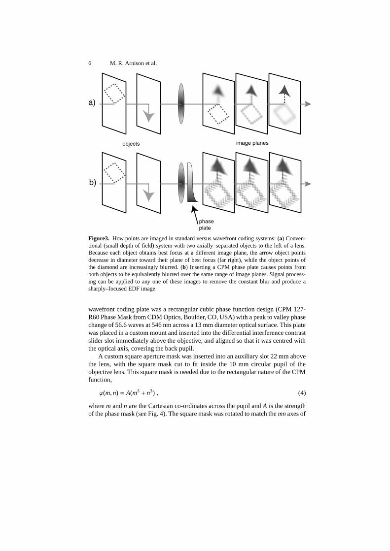
While the optical image produced is quite blurry, it is uniformly blurred over alarge range along the optical axis through the specimen (Fig. 3). From this blurredintermediate image, we can digitally reconstruct a sharp EDF image, using a mea-sured PSF of the system and a single step deconvolution. The waveplate and digitalfilter are chosen to match a particular objective lens and imaging mode, with thedigital filter further calibrated by the measured PSF. Once these steps are carriedout, wavefront coding works well for any typical specimen.

The EDF behaviour relies on modifying the light collection optics only, whichis why it can be used in other imaging systems such as photographic cameras, with-out needing precise control over the illumination light. In epi-fluorescence both theillumination light and the fluorescent light pass through the waveplate. The CPMprovides a beneficial effect on the illumination side, by spreading out the axial rangeof stimulation in the specimen, which will improve the SNR for planes away frombest focus.

2.1 Experimental Method

The experimental setup followed the system outline shown in Fig. 2. We used a ZeissAxioplan microscope with a Plan Neofluar 40x 1.3 NA oil immersion objective. The


objects image planes

phase plate

a)

b)

Figure3. How points are imaged in standard versus wavefront coding systems: (a) Conven-tional (small depth of field) system with two axially–separated objects to the left of a lens.Because each object obtains best focus at a different image plane, the arrow object pointsdecrease in diameter toward their plane of best focus (far right), while the object points ofthe diamond are increasingly blurred. (b) Inserting a CPM phase plate causes points fromboth objects to be equivalently blurred over the same range of image planes. Signal process-ing can be applied to any one of these images to remove the constant blur and produce asharply–focused EDF image

wavefront coding plate was a rectangular cubic phase function design (CPM 127-R60 Phase Mask from CDM Optics, Boulder, CO, USA) with a peak to valley phasechange of 56.6 waves at 546 nm across a 13 mm diameter optical surface. This platewas placed in a custom mount and inserted into the differential interference contrastslider slot immediately above the objective, and aligned so that it was centred withthe optical axis, covering the back pupil.

A custom square aperture mask was inserted into an auxiliary slot 22 mm abovethe lens, with the square mask cut to fit inside the 10 mm circular pupil of theobjective lens. This square mask is needed due to the rectangular nature of the CPMfunction,

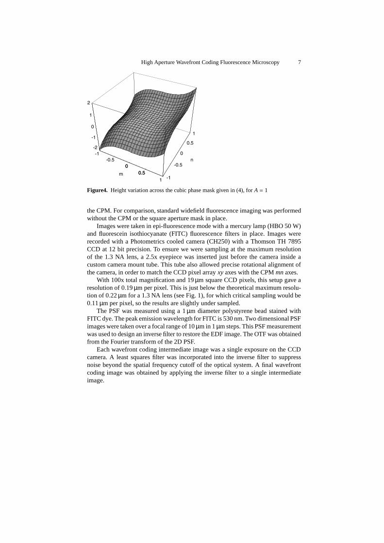
ϕ(m, n) = A(m3 + n3) , (4)

where m and n are the Cartesian co-ordinates across the pupil and A is the strengthof the phase mask (see Fig. 4). The square mask was rotated to match the mn axes of


-1-0.5

00.5

1 -1

-0.5

0

0.5

1

-2

-1

0

1

2

00.5m

n

Figure4. Height variation across the cubic phase mask given in (4), for A = 1

the CPM. For comparison, standard widefield fluorescence imaging was performedwithout the CPM or the square aperture mask in place.

Images were taken in epi-fluorescence mode with a mercury lamp (HBO 50 W)and fluorescein isothiocyanate (FITC) fluorescence filters in place. Images wererecorded with a Photometrics cooled camera (CH250) with a Thomson TH 7895CCD at 12 bit precision. To ensure we were sampling at the maximum resolutionof the 1.3 NA lens, a 2.5x eyepiece was inserted just before the camera inside acustom camera mount tube. This tube also allowed precise rotational alignment ofthe camera, in order to match the CCD pixel array xy axes with the CPM mn axes.

With 100x total magnification and 19 µm square CCD pixels, this setup gave aresolution of 0.19 µm per pixel. This is just below the theoretical maximum resolu-tion of 0.22 µm for a 1.3 NA lens (see Fig. 1), for which critical sampling would be0.11 µm per pixel, so the results are slightly under sampled.

The PSF was measured using a 1 µm diameter polystyrene bead stained withFITC dye. The peak emission wavelength for FITC is 530 nm. Two dimensional PSFimages were taken over a focal range of 10 µm in 1 µm steps. This PSF measurementwas used to design an inverse filter to restore the EDF image. The OTF was obtainedfrom the Fourier transform of the 2D PSF.

Each wavefront coding intermediate image was a single exposure on the CCDcamera. A least squares filter was incorporated into the inverse filter to suppressnoise beyond the spatial frequency cutoff of the optical system. A final wavefrontcoding image was obtained by applying the inverse filter to a single intermediateimage.


10-4

10-3

10-2

10-1

100

0.0 0.2 0.4 0.6 0.8 1.0

|C|

n

widefield zd = 0 µmwidefield zd = 4 µm

CPM zd = 0 µmCPM zd = 4 µm

(e)

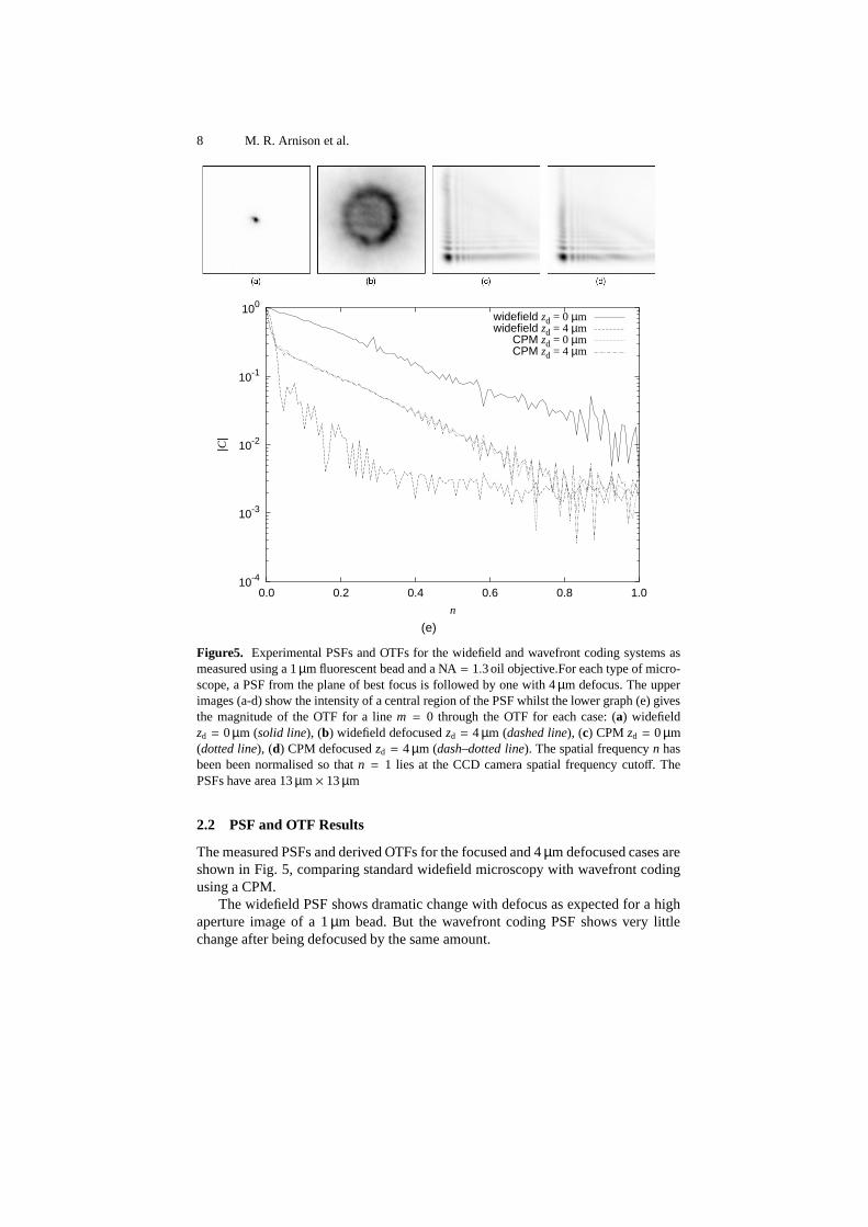
Figure5. Experimental PSFs and OTFs for the widefield and wavefront coding systems asmeasured using a 1 µm fluorescent bead and a NA = 1.3 oil objective.For each type of micro-scope, a PSF from the plane of best focus is followed by one with 4 µm defocus. The upperimages (a-d) show the intensity of a central region of the PSF whilst the lower graph (e) givesthe magnitude of the OTF for a line m = 0 through the OTF for each case: (a) widefieldzd = 0 µm (solid line), (b) widefield defocused zd = 4 µm (dashed line), (c) CPM zd = 0 µm(dotted line), (d) CPM defocused zd = 4 µm (dash–dotted line). The spatial frequency n hasbeen been normalised so that n = 1 lies at the CCD camera spatial frequency cutoff. ThePSFs have area 13 µm × 13 µm

2.2 PSF and OTF Results

The measured PSFs and derived OTFs for the focused and 4 µm defocused cases areshown in Fig. 5, comparing standard widefield microscopy with wavefront codingusing a CPM.

The widefield PSF shows dramatic change with defocus as expected for a highaperture image of a 1 µm bead. But the wavefront coding PSF shows very littlechange after being defocused by the same amount.


(a)

-1.0 -0.5 0.0 0.5 1.0

-1.0 -0.5 0.0 0.5 1.0

-1.0

-0.5

0.0

0.5

1.0

-1.0

-0.5

0.0

0.5

1.0

m

n

(a)

-1.0 -0.5 0.0 0.5 1.0

-1.0 -0.5 0.0 0.5 1.0

-1.0

-0.5

0.0

0.5

1.0

-1.0

-0.5

0.0

0.5

1.0

m

n

-4.0

-3.5

-3.0

-2.5

-2.0

-1.5

-1.0

-0.5

0.0

(b)

-1.0 -0.5 0.0 0.5 1.0

-1.0 -0.5 0.0 0.5 1.0

-1.0

-0.5

0.0

0.5

1.0

-1.0

-0.5

0.0

0.5

1.0

m

n

(b)

-1.0 -0.5 0.0 0.5 1.0

-1.0 -0.5 0.0 0.5 1.0

-1.0

-0.5

0.0

0.5

1.0

-1.0

-0.5

0.0

0.5

1.0

m

n

-3

-2

-1

0

1

2

3

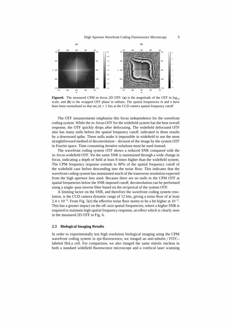
Figure6. The measured CPM in–focus 2D OTF: (a) is the magnitude of the OTF in log10

scale, and (b) is the wrapped OTF phase in radians. The spatial frequencies m and n havebeen been normalised so that |m|, |n| = 1 lies at the CCD camera spatial frequency cutoff

The OTF measurements emphasise this focus independence for the wavefrontcoding system. While the in–focus OTF for the widefield system has the best overallresponse, the OTF quickly drops after defocusing. The widefield defocused OTFalso has many nulls before the spatial frequency cutoff, indicated in these resultsby a downward spike. These nulls make it impossible in widefield to use the moststraightforward method of deconvolution – division of the image by the system OTFin Fourier space. Time consuming iterative solutions must be used instead.

The wavefront coding system OTF shows a reduced SNR compared with thein–focus widefield OTF. Yet the same SNR is maintained through a wide change infocus, indicating a depth of field at least 8 times higher than the widefield system.The CPM frequency response extends to 80% of the spatial frequency cutoff ofthe widefield case before descending into the noise floor. This indicates that thewavefront coding system has maintained much of the transverse resolution expectedfrom the high aperture lens used. Because there are no nulls in the CPM OTF atspatial frequencies below the SNR imposed cutoff, deconvolution can be performedusing a single–pass inverse filter based on the reciprocal of the system OTF.

A limiting factor on the SNR, and therefore the wavefront coding system reso-lution, is the CCD camera dynamic range of 12 bits, giving a noise floor of at least2.4 × 10−4. From Fig. 5(e) the effective noise floor seems to be a bit higher at 10−3.This has a greater impact on the off–axis spatial frequencies, where a higher SNR isrequired to maintain high spatial frequency response, an effect which is clearly seenin the measured 2D OTF in Fig. 6.

2.3 Biological Imaging Results

In order to experimentally test high resolution biological imaging using the CPMwavefront coding system in epi-fluorescence, we imaged an anti-tubulin / FITC–labeled HeLa cell. For comparison, we also imaged the same mitotic nucleus inboth a standard widefield fluorescence microscope and a confocal laser scanning


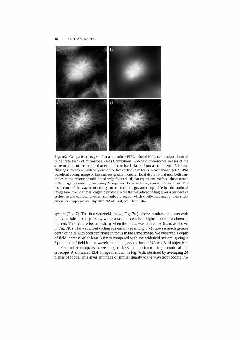
Figure7. Comparison images of an antitubulin / FITC–labeled HeLa cell nucleus obtainedusing three kinds of microscope. (a-b) Conventional widefield fluorescence images of thesame mitotic nucleus acquired at two different focal planes, 6 µm apart in depth. Misfocusblurring is prevalent, with only one of the two centrioles in focus in each image. (c) A CPMwavefront coding image of this nucleus greatly increases focal depth so that now both cen-trioles in the mitotic spindle are sharply focused. (d) An equivalent confocal fluorescenceEDF image obtained by averaging 24 separate planes of focus, spaced 0.5 µm apart. Theresolutions of the wavefront coding and confocal images are comparable but the confocalimage took over 20 times longer to produce. Note that wavefront coding gives a perspectiveprojection and confocal gives an isometric projection, which chiefly accounts for their slightdifference in appearance.Objective NA=1.3 oil, scale bar: 6 µm

system (Fig. 7). The first widefield image, Fig. 7(a), shows a mitotic nucleus withone centriole in sharp focus, while a second centriole higher in the specimen isblurred. This feature became sharp when the focus was altered by 6 µm, as shownin Fig. 7(b). The wavefront coding system image in Fig. 7(c) shows a much greaterdepth of field, with both centrioles in focus in the same image. We observed a depthof field increase of at least 6 times compared with the widefield system, giving a6 µm depth of field for the wavefront coding system for the NA = 1.3 oil objective.

For further comparison, we imaged the same specimen using a confocal mi-croscope. A simulated EDF image is shown in Fig. 7(d), obtained by averaging 24planes of focus. This gives an image of similar quality to the wavefront coding im-


age. However, the confocal system took over 20 times longer to acquire the data forthis image, due to the need to scan the image point in all three dimensions. There isalso a change in projection geometry between the two systems. The confocal EDFimage has orthogonal projection, whereas the wavefront coding EDF image has per-spective projection.

3 Wavefront Coding Theory

In this section we will investigate theoretical models for wavefront coding mi-croscopy. We present a summary of the development of the cubic phase functionand the paraxial theory initially used to model it. We then analyse the system usingvectorial high aperture theory, as is normally required for accuracy with a 1.3 NAlens.

High aperture vectorial models of the PSF for a fluorescence microscope arewell developed [9,23]. The Fourier space equivalent, the OTF, also has a long history[7,13,20]. However, the CPM defined in (4) is an unusual microscope element:

1. Microscope optics usually have radial symmetry around the optical axis, whichthe CPM does not.

2. The CPM gives a very large phase aberration of up to 60 waves, whilst mostaberration models are oriented towards phase strengths on the order of a waveat most.

3. In addition, the CPM spreads the light over a very long focal range, whilst mostPSF calculations can assume the energy drops off very rapidly away from focus.

These peculiarities have meant we needed to take particular care with numericalcomputation in order to ensure accuracy, and in the case of the OTF modeling theradial asymmetry has motivated a reformulation of previous symmetric OTF theory.

3.1 Derivation of the Cubic Phase Function

There are various methods that may be used to derive a pupil phase function whichhas the desired characteristics for EDF imaging. The general form of a phase func-tion in Cartesian co-ordinates is

T (m, n) = exp[ikϕ(m, n)] , (5)

where m, n are the lateral pupil co-ordinates and k = 2π/λ is the wave-number. Thecubic phase function was found by Dowski and Cathey [6] using paraxial opticstheory by assuming the desired phase function is a simple 1D function of the form

ϕ(m) = Amγ, γ , {0, 1}, A , 0 . (6)

By searching for the values of A and γ which give an OTF which does not changethrough focus, they found, using the stationary phase approximation and the ambi-guity function, that the best solution was for A � 20/k and γ = 3. Multiplying outto 2D, this gives the cubic phase function in (4).


3.2 Paraxial Model

Using the Fraunhofer approximation, as suitable for low NA, we can write downa 1D pupil transmission function encompassing the effects of cubic phase (4) anddefocus,

T (m) = exp[ikϕ(m)] exp(im2ψ) , (7)

where ψ is a defocus parameter. We then find the 1D PSF is

E(x) =∫ 1

−1T (m) exp(ixm)dm , (8)

where x is the lateral co-ordinate in the PSF . The 1D OTF is

C(m) =∫ 1

−1T (m′ + m/2)T∗(m′ − m/2)dm′ . (9)

The 2D PSF is simply E(x)E(y).Naturally this 1D CPM gives behaviour in which, in low aperture systems at

least, the lateral x and y imaging axes are independent of each other. This givessignificant speed boosts in digital post–processing. Another important property ofthe CPM is that the OTF does not reach zero below the spatial frequency cutoffwhich means that deconvolution can be carried out in a single step. The lengthyiterative processing of widefield deconvolution is largely due to the many zeros inthe conventional defocused OTF. Another important feature of Fraunhofer optics isthat PSF changes with defocus are limited to scaling changes. Structural changes inthe PSF pattern are not possible.

This paraxial model for the cubic phase mask has been thoroughly verified ex-perimentally for low NA systems [3,24].

3.3 High Aperture PSF Model

We now explore the theoretical behaviour for a high NA cubic phase system. Nor-mally we need high aperture theory for accurate modeling of lenses with NA > 0.5.However large aberrations like our cubic phase mask can sometimes overwhelmthe high NA aspects of focusing. By comparing the paraxial and high NA modelresults we can determine the accuracy of the paraxial approximation for particularwavefront coding systems.

The theory of Richards and Wolf [17] describes how to determine the electricfield near to the focus of a lens which is illuminated by a plane polarised quasi-monochromatic light wave. Their analysis assumes very large values of the Fresnelnumber, equivalent to the Debye approximation. We can then write the equationfor the vectorial amplitude PSF E(x) of a high NA lens illuminated with a planepolarised wave as the Fourier transform of the complex vectorial pupil functionQ(m) [13],

E(x) = − ik2π

∫ ∫ ∫

Q(m) exp(ikm · x)dm . (10)


m=(m,n,s)

x=(x,y,z)

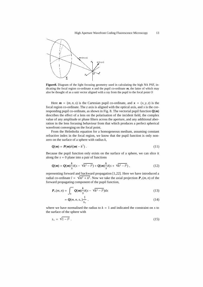
Figure8. Diagram of the light focusing geometry used in calculating the high NA PSF, in-dicating the focal region co-ordinate x and the pupil co-ordinate m, the latter of which mayalso be thought of as a unit vector aligned with a ray from the pupil to the focal point O

Here m = (m, n, s) is the Cartesian pupil co-ordinate, and x = (x, y, z) is thefocal region co-ordinate. The z axis is aligned with the optical axis, and s is the cor-responding pupil co-ordinate, as shown in Fig. 8. The vectorial pupil function Q(m)describes the effect of a lens on the polarisation of the incident field, the complexvalue of any amplitude or phase filters across the aperture, and any additional aber-ration in the lens focusing behaviour from that which produces a perfect sphericalwavefront converging on the focal point.

From the Helmholtz equation for a homogeneous medium, assuming constantrefractive index in the focal region, we know that the pupil function is only non-zero on the surface of a sphere with radius k,

Q(m) = P(m)δ(|m| − k2) . (11)

Because the pupil function only exists on the surface of a sphere, we can slice italong the s = 0 plane into a pair of functions

Q(m) = Q(m)ksδ(s −

√k2 − l2) + Q(m)

ksδ(s +

√k2 − l2) , (12)

representing forward and backward propagation [1,22]. Here we have introduced aradial co-ordinate l =

√m2 + n2. Now we take the axial projection P+(m, n) of the

forward propagating component of the pupil function,

P+(m, n) =∫ ∞

0Q(m)

ksδ(s −

√k2 − l2)ds (13)

= Q(m, n, s+)1s+

, (14)

where we have normalised the radius to k = 1 and indicated the constraint on s tothe surface of the sphere with

s+ =√

1 − l2 . (15)


For incident light which is plane-polarised along the x axis, we can derive avectorial strength function a(m, n), from the strength factors used in the vectorialpoint spread function integrals [12,17,22]

a(m, n) =

(m2s+ + n2)/l2

−mn(1 − s+)/l2

−m

(16)

where we have converted from the spherical polar representation in Richards andWolf to Cartesian co-ordinates.

We can now model polarisation, apodisation and aperture filtering as amplitudeand phase functions over the projected pupil,

P+(m, n) =1s+

a(m, n)S (m, n)T (m, n) (17)

representing forward propagation only (α ≤ π/2), where S (m, n) is the apodisationfunction, and T (m, n) is any complex transmission filter applied across the apertureof the lens. T can also be used to model aberrations.

Microscope objectives are usually designed to obey the sine condition, givingaplanatic imaging [10], for which we write the apodisation as

S (m, n) =√

s+ . (18)

By applying low angle and scalar approximations, we can derive from (17) a parax-ial pupil function,

P+(m, n) � T (m, n) . (19)

Returning to the PSF, we have

E(x) = − ik2π

∫ ∫

Σ

P+(m, n) exp(ikm+ · x)dmdn , (20)

integrated over the projected pupil area Σ. The geometry is shown in Fig. 8. We usem+ = (m, n, s+) to indicate that m is constrained to the pupil sphere surface.

For a clear circular pupil of aperture half–angle α, the integration area Σcirc isdefined by

0 ≤ l ≤ sinα , (21)

while for a square pupil which fits inside that circle, the limits on Σsq are

|m| ≤ sinα/√

2|n| ≤ sinα/

√2. (22)

The transmission function T is unity for a standard widefield system with noaberrations, while for a cubic phase system (4) and (5) give

Tc(m, n) = exp[ikA(m3 + n3)] . (23)


3.4 High Aperture OTF Model

A high aperture analysis of the OTF is important, because the OTF has proven to bemore useful than the PSF for design and analysis of low aperture wavefront codingsystems. For full investigation of the spatial frequency response of a high aperturemicroscope, we would normally look to the 3D OTF [7,13,19,20]. We have recentlypublished a method for calculating the 3D OTF suitable for arbitrary pupil filters[1] which can be applied directly to find the OTF for a cubic phase plate. But sincean EDF system involves recording a single image at one focal depth, a frequencyanalysis of the 2D PSF at that focal plane is more appropriate. This can be performedefficiently using a high NA vectorial adaptation of 2D Fourier optics [22].

This adaptation relies on the Fourier projection–slice theorem [2], which statesthat a slice through real space is equivalent to a projection in Fourier space:

f (x, y, 0)⇐⇒∫

F(m, n, s)ds (24)

where F(m, n, s) is the Fourier transform of f (x, y, z). We have already obtainedthe projected pupil function P+(m, n) in (17). Taking the 2D Fourier transform andapplying (24) gives the PSF in the focal plane

E(x, y, 0)⇐⇒ P+(m, n) . (25)

Since fluorescence microscopy is incoherent, we then take the intensity and 2DFourier transform once more to obtain the OTF of that slice of the PSF

C(m, n)⇐⇒ |E(x, y, 0)|2 . (26)

We can implement this approach using 2D fast Fourier transforms to quickly calcu-late the high aperture vectorial OTF for the focal plane.

3.5 Defocused OTF and PSF

To investigate the EDF performance, we need to calculate the defocused OTF. De-focus is an axial shift zd of the point source being imaged relative to the focal point.By the Fourier shift theorem, a translation zd of the PSF is equivalent to a linearphase shift in the 3D pupil function,

E(x, y, 0 + zd)⇐⇒ exp(ikszd)Q(m, n, s) . (27)

Applying the projection-slice theorem as before gives a modified version of (25)

E(x, y, zd)⇐⇒∫

exp(ikszd)Q(m, n, s)ds . (28)

allowing us to isolate a pupil transmission function that corresponds to a given de-focus zd,

Td(m, n, zd) = exp(iks+zd) , (29)


Table1. Optical parameters used for PSF and OTF simulations

Optical parameter Simulation valueWavelength 530 nmNumerical aperture NA = 1.3 oilOil refractive index n1 = 1.518Aperture half angle α = π/3Pupil shape SquarePupil width 7.1 mmCubic phase strength 25.8 waves peak to valley

which we incorporate into the projected pupil function P+(m, n) from (17), giving

P+(m, n, zd) =1s+

a(m, n)S (m, n)Td(m, n, zd)Tc(m, n) . (30)

If we assume a low aperture pupil, we can approximate (15) to second order, givingthe well known paraxial aberration function for defocus

Td(m, n, zd) � exp

(

−ikzdl2

2

)

. (31)

Finally, using F to denote a Fourier transform, we write down the full algorithm forcalculating the OTF of a transverse slice through the PSF:

C(m, n, zd) = F −1{

|F [P+(m, n, zd)]|2}

. (32)

It is convenient to calculate the defocused PSF using the first step of the same ap-proach:

E(x, y, zd) = F [P+(m, n, zd)] . (33)

3.6 Simulation Results

We have applied this theoretical model to simulate the wavefront coding experi-ments described earlier, using the parameters given in Table 1. The theoretical as-sumption that the incident light is plane polarised corresponds to the placement ofan analyser in the microscope beam path. This polarisation explains some xy asym-metry in the simulation results.

Due to the large phase variation across the pupil, together with the large defocusdistances under investigation, a large number of samples of the cubic phase functionwere required to ensure accuracy and prevent aliasing. We created a 2D array with10242 samples of the pupil function P+ from (30) using (22) for the aperture cutoff.We then padded this array out to 40962 to allow for sufficient sampling of the result-ing PSF, before employing the algorithms in (33) and (32) to calculate the PSF andOTF respectively. Using fast Fourier transforms, each execution of (32) took about8 minutes on a Linux Athlon 1.4 GHz computer with 1 GB of RAM.


10-4

10-3

10-2

10-1

100

0.0 0.2 0.4 0.6 0.8 1.0 1.2 1.4 1.6

|C|

l

vectorialparaxial

(a)

10-4

10-3

10-2

10-1

100

0.0 0.2 0.4 0.6 0.8 1.0 1.2 1.4 1.6

|C|

l

vectorialparaxial

(b)

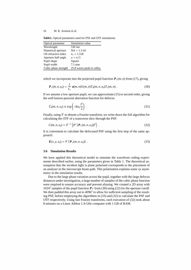
Figure9. A comparison of widefield (no CPM) OTFs using our vectorial (solid line) andparaxial (dashed line) simulations: (a) in–focus at zd = 0 µm and (b) defocused to zd = 4 µm.For a diagonal line through the OTF along m = n, we have plotted the value of the 2Dprojected OTF for each case. While the structure of the in–focus OTF curves is similar for thetwo models, the relative difference between them increases with spatial frequency, reachingover 130% at the cutoff. Once defocus is applied, the two models predict markedly differentfrequency response in both structure and amplitude

The wavefront coding inverse filter for our experiments was derived from thetheoretical widefield (no CPM) OTF and the measured CPM OTF. The discrepancyin the focal plane theoretical widefield OTF between the paraxial approximation


x

y

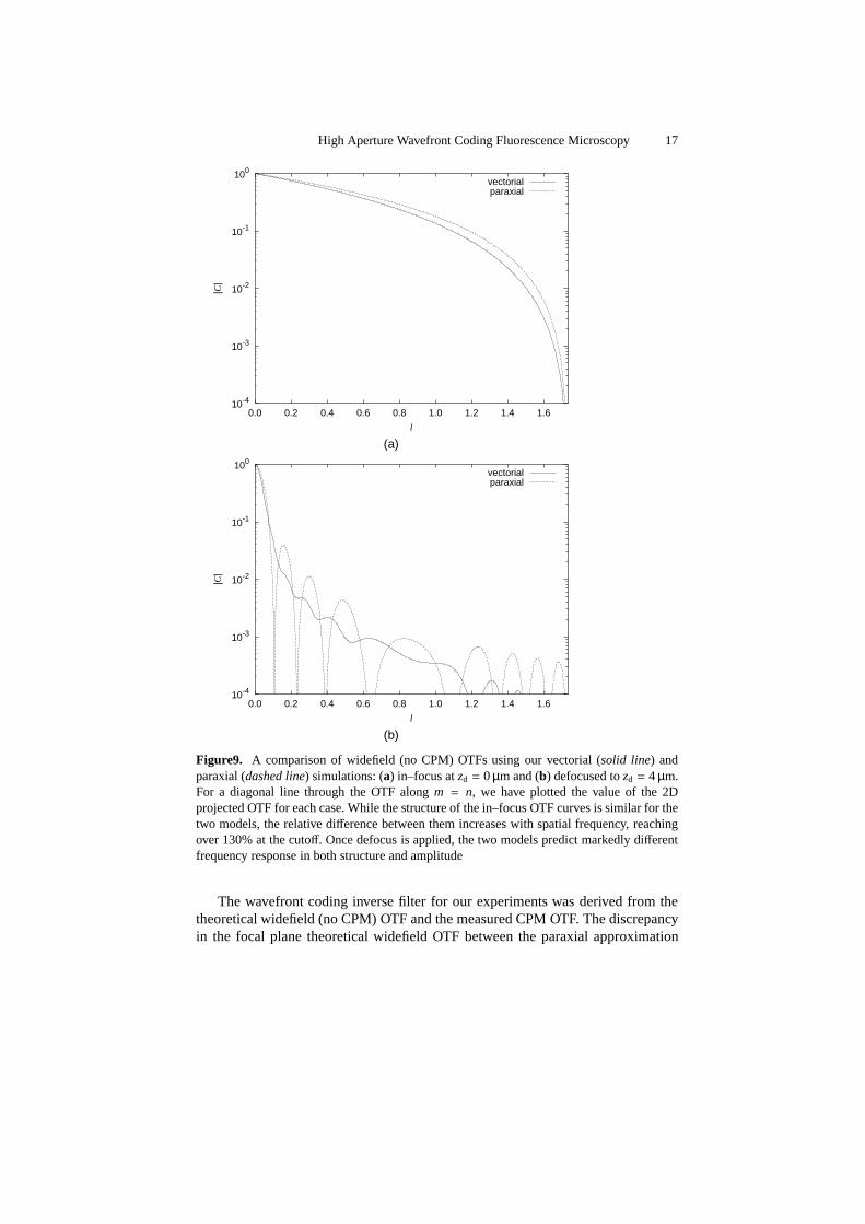
Figure10. The simulated vectorial high aperture PSF for widefield and wavefront coding,showing the effect of defocus: (a) widefield in–focus zd = 0 µm, (b) widefield defocusedzd = 4 µm, (c) CPM in–focus zd = 0 µm, (d) CPM defocused zd = 4 µm. This amount ofdefocus introduces very little discernible difference between the CPM PSFs. Indeed paraxialCPM simulations (not shown here) are also similar in structure. The PSFs shown have thesame area as Fig. 5 (13 µm×13 µm). The incident polarisation is in the x direction. The imagesare normalised to the peak intensity of each case. Naturally the peak intensity decreases withdefocus, but much less rapidly in the CPM system

(a)

-1.0 -0.5 0.0 0.5 1.0

-1.0 -0.5 0.0 0.5 1.0

-1.0

-0.5

0.0

0.5

1.0

-1.0

-0.5

0.0

0.5

1.0

m

n

(a)

-1.0 -0.5 0.0 0.5 1.0

-1.0 -0.5 0.0 0.5 1.0

-1.0

-0.5

0.0

0.5

1.0

-1.0

-0.5

0.0

0.5

1.0

m

n

-4.0

-3.5

-3.0

-2.5

-2.0

-1.5

-1.0

-0.5

0.0

(b)

-1.0 -0.5 0.0 0.5 1.0

-1.0 -0.5 0.0 0.5 1.0

-1.0

-0.5

0.0

0.5

1.0

-1.0

-0.5

0.0

0.5

1.0

m

n(b)

-1.0 -0.5 0.0 0.5 1.0

-1.0 -0.5 0.0 0.5 1.0

-1.0

-0.5

0.0

0.5

1.0

-1.0

-0.5

0.0

0.5

1.0

m

n

-3

-2

-1

0

1

2

3

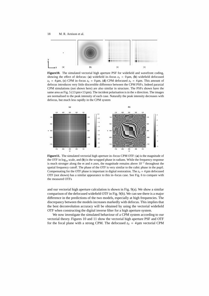
Figure11. The simulated vectorial high aperture in–focus CPM OTF: (a) is the magnitude ofthe OTF in log10 scale, and (b) is the wrapped phase in radians. While the frequency responseis much stronger along the m and n axes, the magnitude remains above 10−3 throughout thespatial frequency cutoff. The phase of the OTF is very similar to the cubic phase in the pupil.Compensating for the OTF phase is important in digital restoration. The zd = 4 µm defocusedOTF (not shown) has a similar appearance to this in–focus case. See Fig. 6 to compare withthe measured OTFs

and our vectorial high aperture calculation is shown in Fig. 9(a). We show a similarcomparison of the defocused widefield OTF in Fig. 9(b). We can see there is a majordifference in the predictions of the two models, especially at high frequencies. Thediscrepancy between the models increases markedly with defocus. This implies thatthe best deconvolution accuracy will be obtained by using the vectorial widefieldOTF when constructing the digital inverse filter for a high aperture system.

We now investigate the simulated behaviour of a CPM system according to ourvectorial theory. Figures 10 and 11 show the vectorial high aperture PSF and OTFfor the focal plane with a strong CPM. The defocused zd = 4 µm vectorial CPM


10-4

10-3

10-2

10-1

100

0.0 0.2 0.4 0.6 0.8 1.0 1.2 1.4 1.6

|C|

l

zd = 0 µmzd = 2 µmzd = 4 µm

(a)

10-4

10-3

10-2

10-1

100

0.0 0.2 0.4 0.6 0.8 1.0 1.2 1.4 1.6

|C|

l

zd = 0 µmzd = 2 µmzd = 4 µm

(b)

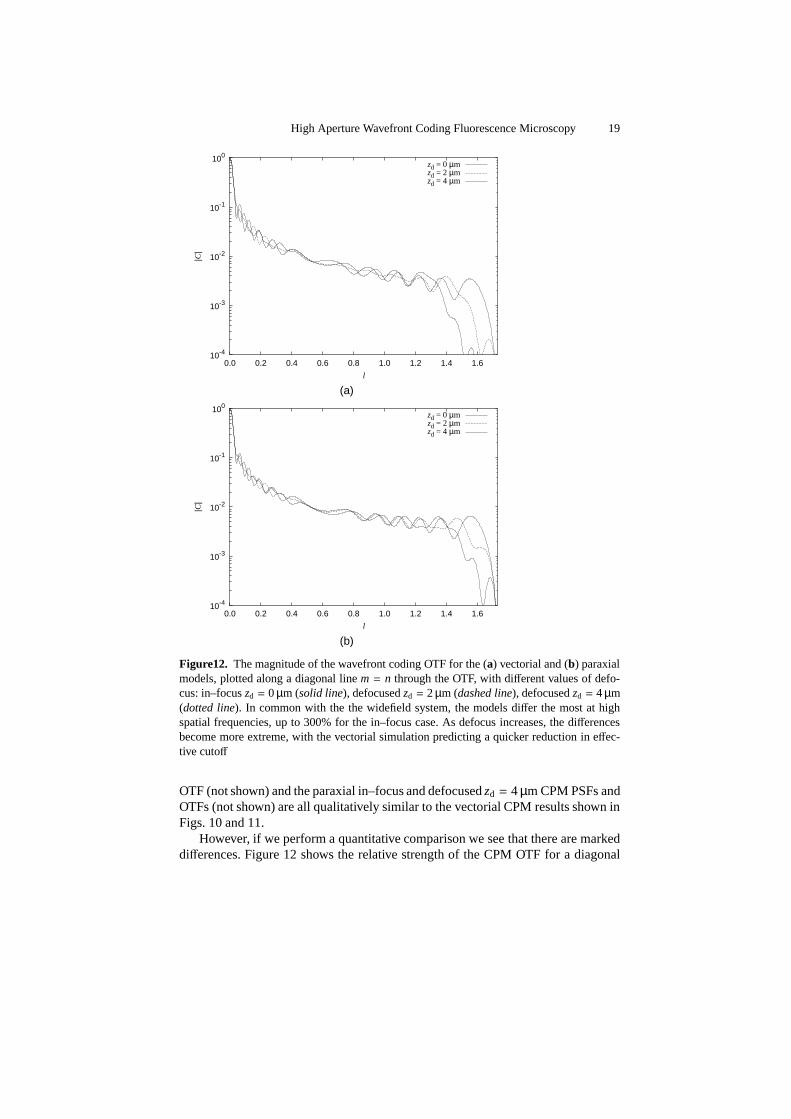
Figure12. The magnitude of the wavefront coding OTF for the (a) vectorial and (b) paraxialmodels, plotted along a diagonal line m = n through the OTF, with different values of defo-cus: in–focus zd = 0 µm (solid line), defocused zd = 2 µm (dashed line), defocused zd = 4 µm(dotted line). In common with the the widefield system, the models differ the most at highspatial frequencies, up to 300% for the in–focus case. As defocus increases, the differencesbecome more extreme, with the vectorial simulation predicting a quicker reduction in effec-tive cutoff

OTF (not shown) and the paraxial in–focus and defocused zd = 4 µm CPM PSFs andOTFs (not shown) are all qualitatively similar to the vectorial CPM results shown inFigs. 10 and 11.

However, if we perform a quantitative comparison we see that there are markeddifferences. Figure 12 shows the relative strength of the CPM OTF for a diagonal


cross section. The differences between the models are similar to the widefield OTFin Fig. 9(a) for the in–focus case, with up to 100% difference at high spatial fre-quencies. However, as the defocus increases, the structure of the vectorial CPM OTFbegins to diverge from the paraxial model, as well as the point where the strengthdrops below 10−4. This is still a much lower discrepancy than the widefield modelfor similar amounts of defocus, as is clear by comparison with Fig. 9.

These plots allow us to assess the SNR requirements for recording images withmaximum spatial frequency response. For both widefield and CPM systems, theexperimental dynamic range will place an upper limit on the spatial frequency re-sponse. In widefield a 103 SNR of will capture nearly all spatial frequencies up tothe cutoff (see Fig. 9(a)), allowing for good contrast throughout. Further increases inSNR will bring rapidly diminishing returns, only gradually increasing the maximumspatial frequency response.

For CPM imaging the same 103 SNR will produce good contrast only for lowspatial frequencies, with the middle frequencies lying less than a factor of ten abovethe noise floor, and the upper frequencies dipping below it. However, a SNR of 104

will allow a more reasonable contrast level across the entire OTF. For this reason,a 16 bit camera, together with other noise control measures, is needed for a CPMsystem to achieve the full resolution potential of high aperture lenses. This need forhigh dynamic range creates a trade off for rapid imaging of living specimens – fasterexposure times will reduce the SNR and lower the resolution.

Arguably the most important OTF characteristic used in the EDF digital decon-volution is the phase. As can be seen from Fig. 11 the CPM OTF phase oscillatesheavily due to the strong cubic phase. This corresponds to the numerous contrastreversals in the PSF. The restoration filter is derived from the OTF, and therefore ac-curate phase in the OTF is needed to ensure that any contrast reversals are correctlyrestored.

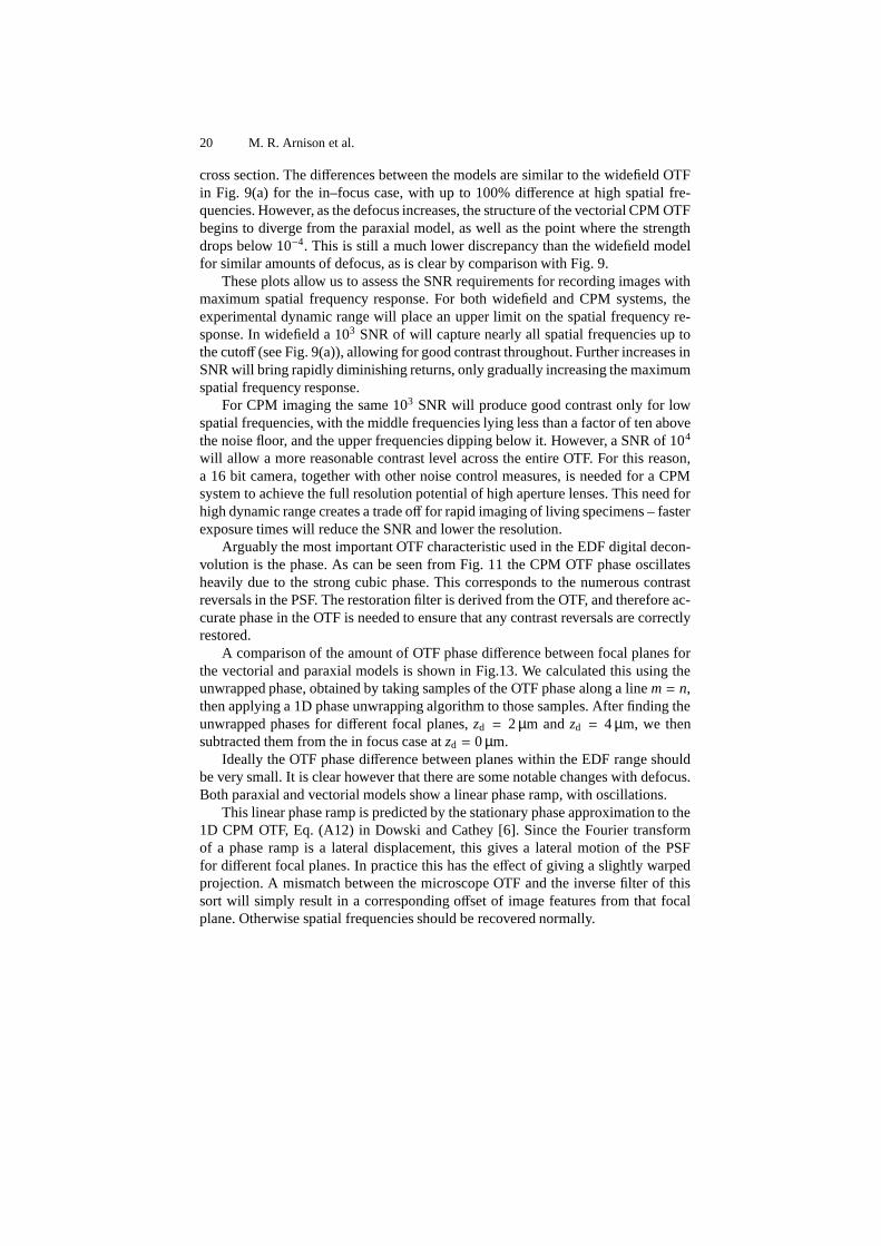
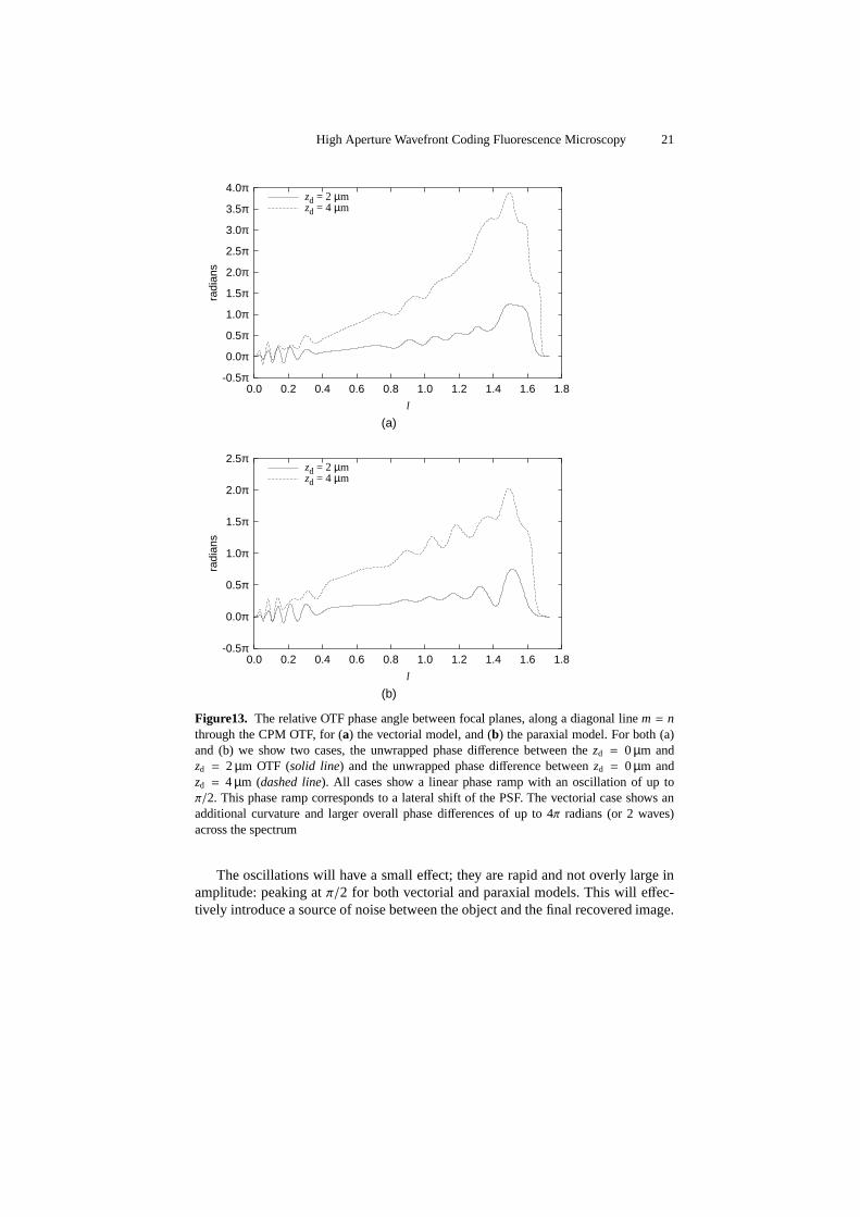
A comparison of the amount of OTF phase difference between focal planes forthe vectorial and paraxial models is shown in Fig.13. We calculated this using theunwrapped phase, obtained by taking samples of the OTF phase along a line m = n,then applying a 1D phase unwrapping algorithm to those samples. After finding theunwrapped phases for different focal planes, zd = 2 µm and zd = 4 µm, we thensubtracted them from the in focus case at zd = 0 µm.

Ideally the OTF phase difference between planes within the EDF range shouldbe very small. It is clear however that there are some notable changes with defocus.Both paraxial and vectorial models show a linear phase ramp, with oscillations.

This linear phase ramp is predicted by the stationary phase approximation to the1D CPM OTF, Eq. (A12) in Dowski and Cathey [6]. Since the Fourier transformof a phase ramp is a lateral displacement, this gives a lateral motion of the PSFfor different focal planes. In practice this has the effect of giving a slightly warpedprojection. A mismatch between the microscope OTF and the inverse filter of thissort will simply result in a corresponding offset of image features from that focalplane. Otherwise spatial frequencies should be recovered normally.


-0.5π

0.0π

0.5π

1.0π

1.5π

2.0π

2.5π

3.0π

3.5π

4.0π

0.0 0.2 0.4 0.6 0.8 1.0 1.2 1.4 1.6 1.8

radi

ans

l

zd = 2 µmzd = 4 µm

(a)

-0.5π

0.0π

0.5π

1.0π

1.5π

2.0π

2.5π

0.0 0.2 0.4 0.6 0.8 1.0 1.2 1.4 1.6 1.8

radi

ans

l

zd = 2 µmzd = 4 µm

(b)

Figure13. The relative OTF phase angle between focal planes, along a diagonal line m = nthrough the CPM OTF, for (a) the vectorial model, and (b) the paraxial model. For both (a)and (b) we show two cases, the unwrapped phase difference between the zd = 0 µm andzd = 2 µm OTF (solid line) and the unwrapped phase difference between zd = 0 µm andzd = 4 µm (dashed line). All cases show a linear phase ramp with an oscillation of up toπ/2. This phase ramp corresponds to a lateral shift of the PSF. The vectorial case shows anadditional curvature and larger overall phase differences of up to 4π radians (or 2 waves)across the spectrum

The oscillations will have a small effect; they are rapid and not overly large inamplitude: peaking at π/2 for both vectorial and paraxial models. This will effec-tively introduce a source of noise between the object and the final recovered image.


Whilst these oscillations are not predicted by the stationary phase approximation,they are still evident for the paraxial model.

The most dramatic difference between the two models is in the curvature ofthe vectorial case, which is particularly striking in the zd = 4 µm plane, and notdiscernible at all in the paraxial case (Fig.13). This primary effect of this curvaturewill be to introduce some additional blurring of specimen features in the zd = 4 µmplane, which the inverse filter will not be able to correct. The total strength of thiscurvature at zd = 4 µm is about 2π across the complete m = n line, or one wave,which is a significant aberration.

3.7 Discussion

The CPM acts as a strong aberration which appears to dominate both the effects ofdefocus and of vectorial high aperture focusing. The paraxial approximation cer-tainly loses accuracy for larger values of defocus, but not nearly so much as in thedefocused widefield case. Yet significant differences remain between the two mod-els, notably a one wave curvature aberration in the vectorial case, and this suggeststhat vectorial high aperture theory will be important in the future design of highaperture wavefront coding systems.

We can also look at the two models as providing an indication of the difference inperformance of CPM wavefront coding between low aperture and high aperture sys-tems. The curvature aberration in the high aperture case varies with defocus, whichmeans that it cannot be incorporated into any 2D digital deconvolution scheme. Thiseffectively introduces an additional blurring of specimen features in planes awayfrom focus, lowering the depth of field boost achieved with the same CPM strengthin a low aperture wavefront coding system.

In general the CPM performs a little better at low apertures for EDF applications.But the high aperture CPM system still maintains useful frequency response acrossthe full range of an equivalent widefield system, especially for on–axis frequencies.

4 Conclusion

Wavefront coding is a new approach to microscopy. Instead of avoiding aberra-tions, we deliberately create and exploit them. The aperture of the imaging lensstill places fundamental limits on performance. However wavefront coding allowsus to trade off those limits between the different parameters we need for a givenimaging task. Focal range, signal to noise, mechanical focus scanning speed andmaximum frequency response are all negotiable using this digital–optical approachto microscopy.

The high aperture experimental results presented here point to the significantpromise of wavefront coding. The theoretical simulations predict an altered be-haviour for high apertures, which will become more important with higher SNRimaging systems. For large values of defocus, these results predict a tighter limit


on the focal range of EDF imaging than is the case for paraxial systems, as well asadditional potential for image artefacts due to aberrations.

The fundamental EDF behaviour remains in force at high apertures, as demon-strated by both experiment and theory. This gives a solid foundation to build on. TheCPM was part of the first generation wavefront coding design. Using simulations,new phase mask designs can be tested for performance at high apertures before fab-rication. With this knowledge, further development of wavefront coding techniquesmay be carried out, enhancing its use at high apertures.

Acknowledgments

We would like to thank W. Thomas Cathey and Edward R. Dowski Jr. of CDMOptics Inc, Boulder, CO, USA. Experimental assistance was provided by ElanorKable, Theresa Dibbayawan, David Philp and Janey Lin at the University of Sydneyand Claude Rosignol at Colorado University.

References

1. Matthew R. Arnison and Colin J. R. Sheppard. A 3D vectorial optical transfer functionsuitable for arbitrary pupil functions. Opt. Commun., 211(1-6):45–55, 2002.

2. R. N. Bracewell. Two-dimensional imaging. Prentice Hall, Englewood Cliffs, NJ, USA,1995.

3. Sara Bradburn, W. Thomas Cathey, and Edward R. Dowski, Jr. Realizations of focusinvariance in optical-digital systems with wave-front coding. App. Opt., 36(35):9157–9166, 1997.

4. Juan Campos, Juan C. Escalera, Colin J. R. Sheppard, and María J. Yzuel. Axiallyinvariant pupil filters. J. Mod. Optics, 47(1):57–68, 2000.

5. Wanli Chi and Nicholas George. Electronic imaging using a logarithmic asphere. Opt.Lett., 26(12):875–877, 2001.

6. Edward R. Dowski, Jr. and W. Thomas Cathey. Extended depth of field through wave-front coding. App. Opt., 34(11):1859–1866, 10 April 1995.

7. B. R. Frieden. Optical transfer of the three-dimensional object. J. Opt. Soc. Am., 57:56–66, 1967.

8. G. Häusler. A method to increase the depth of focus by two step image processing. Opt.Commun., 6(1):38–42, 1972.

9. P. D. Higdon, Peter Török, and Tony Wilson. Imaging properties of high aperture multi-photon fluorescence scanning optical microscopes. J. Microsc., 193(2):127–141, Febru-ary 1999.

10. H. H. Hopkins. The Airy disc formula for systems of high relative aperture. Proc. Phys.Soc., 55:116, 1943.

11. R. Juškaitis, M. A. A. Neil, F. Massoumian, and T. Wilson. Strategies for wide-fieldextended focus microscopy. In Focus on microscopy, Amsterdam, April 2001.

12. M Mansuripur. Distribution of light at and near the focus of high-numerical-apertureobjectives. J. Opt. Soc. Am. A, 3(12):2086–2093, 1986.

13. C W McCutchen. Generalized aperture and the three-dimensional diffraction image. J.Opt. Soc. Am., 54:240–244, 1964.


14. Jorge Ojeda-Castañeda, R. Ramos, and A. Noyola-Isgleas. High focal depth by apodiza-tion and digital restoration. Appl. Opt., 27:2583–2586, 1988.

15. Jorge Ojeda-Castañeda, E. Tepichin, and A. Diaz. Arbitrarily high focal depth with aquasioptimum real and positive transmittance apodizer. Appl. Opt., 28(13):2666–2670,1989.

16. P. Potuluri, Matthew Fetterman, and David Brady. High depth of field microscopic imag-ing using an interferometric camera. Opt. Express, 8(11):624, May 2001.

17. B. Richards and E. Wolf. Electromagnetic diffraction in optical systems II. Structure ofthe image field in aplanatic systems. Proc. Roy. Soc. A, 253:358–379, 1959.

18. C. J. R. Sheppard. Depth of field in optical microscopy. J. Microsc., 149:73–75, 1988.19. C. J. R. Sheppard and C. J. Cogswell. Confocal microscopy, chapter Three-dimensional

imaging in confocal microscopy, pages 143–169. Academic Press, London, 1990.20. C J R Sheppard, M Gu, Y Kawata, and S Kawata. Three-dimensional transfer functions

for high aperture systems obeying the sine condition. J. Opt. Soc. Am. A, 11:593–598,1994.

21. C. J. R. Sheppard, D. K. Hamilton, and I. J. Cox. Optical microscopy with extendeddepth of field. Proc. R. Soc. Lond. A, A387:171–186, 1983.

22. C. J. R. Sheppard and K. G. Larkin. Vectorial pupil functions and vectorial transferfunctions. Optik, 107(2):79–87, 1997.

23. P. Török, P. Varga, Z. Laczik, and G. R. Booker. Electromagnetic diffraction of lightfocussed through a planar interface between materials of mismatched refractive indices:an integral representation. J. Opt. Soc. Am. A, 12(2):325–332, 1995.

24. Sara C. Tucker, W. Thomas Cathey, and Edward R. Dowski, Jr. Extended depth offield and aberration control for inexpensive digital microscope systems. Optics Express,4(11):467–474, 1999.

25. W T Welford. Use of annular apertures to increase focal depth. J. Opt. Soc. Am.,50(8):749–753, 1960.

26. T. Wilson, MAA. Neil, and F. Massoumian. Point spread functions with extended depthof focus. In Proc. SPIE, volume 4621, pages 28–31, San Jose, CA, USA, January 2002.

Documents

Wavefront Coding Fluorescence Microscopy Using High Aperture Lenses