Wave-activity conservation laws and stability theorems for

Wave-activity conservation laws and stability theorems for semi-geostrophic dynamics: part 1. pseudomomentum-based theory

Article

Published Version

Kushner, P. J. and Shepherd, T. G. (1995) Wave-activity conservation laws and stability theorems for semi-geostrophic dynamics: part 1. pseudomomentum-based theory. Journal Of Fluid Mechanics, 290. pp. 67-104. ISSN 0022-1120 doi: https://doi.org/10.1017/S0022112095002424 Available at http://centaur.reading.ac.uk/32895/

It is advisable to refer to the publisher’s version if you intend to cite from the work. See Guidance on citing .Published version at: http://dx.doi.org/10.1017/S0022112095002424

To link to this article DOI: http://dx.doi.org/10.1017/S0022112095002424

Publisher: Cambridge University Press

All outputs in CentAUR are protected by Intellectual Property Rights law,

http://centaur.reading.ac.uk/71187/10/CentAUR%20citing%20guide.pdf

including copyright law. Copyright and IPR is retained by the creators or other copyright holders. Terms and conditions for use of this material are defined in the End User Agreement .

www.reading.ac.uk/centaur

CentAUR

Central Archive at the University of Reading

Reading’s research outputs online

http://www.reading.ac.uk/centaur

http://centaur.reading.ac.uk/licence

J. Fluid Mech. (1995), 001. 290, pp. 67-104 Copyright Q 1995 Cambridge University Press

Wave-activity conservation laws and stability theorems for semi-geostrophic dynamics. Part 1.

Pseudomomentum-based theory By PAUL J. KUSHNER A N D THEODORE G. SHEPHERD

Department of Physics, University of Toronto, Toronto, Canada MSS 1A7

(Received 2 February 1994 and in revised form 22 August 1994)

67

There exists a well-developed body of theory based on quasi-geostrophic (QG) dynamics that is central to our present understanding of large-scale atmospheric and oceanic dynamics. An important question is the extent to which this body of theory may generalize to more accurate dynamical models. As a first step in this process, we here generalize a set of theoretical results, concerning the evolution of disturbances to prescribed basic states, to semi-geostrophic (SG) dynamics. SG dynamics, like QG dynamics, is a Hamiltonian balanced model whose evolution is described by the material conservation of potential vorticity, together with an invertibility principle relating the potential vorticity to the advecting fields. SG dynamics has features that make it a good prototype for balanced models that are more accurate than QG dynamics.

In the first part of this two-part study, we derive a pseudomomentum invariant for the SG equations, and use it to obtain: (i) linear and nonlinear generalized Charney-Stern theorems for disturbances to parallel flows; (ii) a finite-amplitude local conservation law for the invariant, obeying the group-velocity property in the WKB limit ; and (iii) a wave-mean-flow interaction theorem consisting of generalized Eliassen-Palm flux diagnostics, an elliptic equation for the stream-function tendency, and a non-acceleration theorem. All these results are analogous to their QG forms.

The pseudomomentum invariant - a conserved second-order disturbance quantity that is associated with zonal symmetry - is constructed using a variational principle in a similar manner to the QG calculations. Such an approach is possible when the equations of motion under the geostrophic momentum approximation are transformed to isentropic and geostrophic coordinates, in which the ageostrophic advection terms are no longer explicit. Symmetry-related wave-activity invariants such as the pseudomomentum then arise naturally from the Hamiltonian structure of the SG equations. We avoid use of the so-called ‘massless layer’ approach to the modelling of isentropic gradients at the lower boundary, preferring instead to incorporate explicitly those boundary contributions into the wave-activity and stability results. This makes the analogy with QG dynamics most transparent.

This paper treats the f-plane Boussinesq form of SG dynamics, and its recent extension to ,&plane, compressible flow by Magnusdottir & Schubert. In the limit of small Rossby number, the results reduce to their respective QG forms. Novel features particular to SG dynamics include apparently unnoticed lateral boundary stability criteria in (i), and the necessity of including additional zonal-mean eddy correlation terms besides the zonal-mean potential vorticity fluxes in the wave-mean-flow balance in (iii).

In the companion paper, wave-activity conservation laws and stability theorems based on the SG form of the pseudoenergy are presented.

68 P . J . Kushner and T . G . Shepherd

1. Introduction A classical and important area of research in fluid mechanics concerns the evolution

of disturbances to prescribed basic states. Notable examples of theoretical questions falling within this framework include the propagation of waves in inhomogeneous media, the stability or instability of basic states, and the driving of mean-flow changes by wave transience and dissipation. Within the field of large-scale atmospheric dynamics, there is a well-developed body of such theory based on quasi-geostrophic (QG) dynamics. It includes Eliassen-Palm (E-P) flux diagnostics (Andrews & McIntyre 1976, 1978); finite-amplitude wave-activity conservation laws (McIntyre & Shepherd 1987); nonlinear stability theorems for parallel and/or steady flows (Holm et al. 1985; McIntyre & Shepherd 1987; Shepherd 1989, hereinafter referred to as S89); and rigorous saturation bounds on baroclinic instabilities (Shepherd 1988, 1993 ; S89). Aspects of this theory have been successfully applied to diagnose the role of eddies in simple models, primitive-equations general circulation models, and observations (e.g. Edmon, Hoskins & McIntyre 1980; Dunkerton, Hsu & McIntyre 1981 ; Hoskins 1983; Held & Hoskins 1985; Randel & Held 1991).

It is nevertheless widely recognized that QG theory has serious quantitative limitations. Therefore it is natural to ask to what extent the body of theory described above generalizes to other, more complicated dynamical models. To answer this question, one must consider what is fundamental about this theory, and what is specific to the QG model. Despite its seemingly broad range of form and application, it turns out that the above-mentioned QG theory has two related, central features, within which everything may be concisely understood. First, the dynamics can be described in terms of material advection of potential vorticity (PV), together with some sort of ‘invertibility ’ or ‘balance’ relation that determines the advecting velocity given the PV (see e.g. Hoskins, McIntyre & Robertson 1985); and second, there is an underlying Hamiltonian structure which provides conservation laws for so-called ‘ wave-activity ’ invariants such as the pseudomomentum and pseudoenergy (see e.g. Shepherd 1990). Both of these features are exact, finite-amplitude properties of the dynamics.

Seen from this perspective, it seems plausible that the wave-activity conservation laws and stability theorems that underlie the modern understanding of QG dynamics may generalize to other models that are more accurate, yet which contain the two ingredients of balanced dynamics and Hamiltonian structure. The derivation of such models is an active topic of current research. At the present time, there is only one such model : semi-geostrophic (SG) dynamics.

The SG model was first introduced by Hoskins (1975) in the context of thef-plane Boussinesq equations. It is based on the ‘ geostrophic momentum’ approximation of Eliassen (1948), and has been widely used to study the dynamics of mesoscale phenomena. More recently, the SG model has been extended to the B-plane compressible equations by Magnusdottir & Schubert (1990, hereinafter referred to as MSc90).

The purpose of the present study is to generalize the well-established body of QG theory consisting of wave-activity conservation laws and stability theorems to these two SG models. While the study is motivated by analogies between QG and SG dynamics, its length is largely due to the differences between them. Both models are described by material conservation of PV, with appropriate time-evolution equations for quantities at the boundaries. In both models, an invertibility principle relates the advecting stream-function potential to the PV and boundary terms. However, the SG model differs from the QG one in its use of a coordinate transformation to express the

Wave-activity conservation laws for semi-geostrophic dynamics. Part I 69

invertibility principle, in the nonlinear nature of the principle, and, most prob- lematically, in its form of the boundary conditions. The coordinate transformation to isentropic geostrophic coordinates (IGC) is used to reduce the SG model to its simplest form. However, the transformation introduces complications into the dynamics at fixed geometric bounding surfaces. In the transformed space, these surfaces become dynamic quantities whose positions evolve with time. This variability has been explicitly incorporated, where feasible, into the theory.

The paper is structured as follows. We first introduce the reader to SG dynamics, establishing notation and providing some insight into its properties. In $2, the f-plane Boussinesq system of Hoskins (1975) is introduced and transformed to IGC. The set of equations (2.18)-(2.20) summarize the prognostic interior and boundary equations and the diagnostic invertibility relation. Section 3 motivates the rest of the paper by using direct methods to derive a version of the Charney-Stern theorem for disturbances to parallel flows that includes explicit boundary contributions from both vertical and lateral bounding surfaces. The theorem is expressed in terms of a conservation law (equation (3.10) or (3.12)) that turns out to be an expression of linearized pseudomomentum conservation.

We then proceed with a systematic theoretical treatment. In $4, the conservation laws for the system are derived in physical coordimtes. In $ 5 , the pseudomomentum - i.e. the wave-activity invariant for disturbances to parallel flows that is related to the zonal symmetry of the system-is derived from a variational principle, after a discussion of the nature of the basic state and the variational problem at the boundaries. In $6, a nonlinear generalization of the Charney-Stern theorem is derived, with some restrictions on the nature of the perturbations at the boundaries. In $7, a local form of the wave-activity conservation law is developed, and the group-velocity property verified for the particular form of the flux. In $8, wave-mean-flow E-P flux diagnostics are developed, including a non-acceleration theorem. In $ 9, the results of 82-8 are extended to the /3-plane compressible system of MSc90. The results are summarized, and their relevance and limitations discussed, in $ 10.

In the sequel to this paper (Kushner & Shepherd 1995), wave-activity conservation laws and stability theorems based on the SG form of the pseudoenergy are presented.

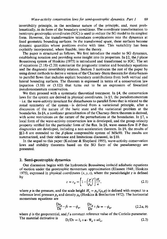
2. Semi-geostrophic dynamics Our discussion begins with the hydrostatic Boussinesq inviscid adiabatic equations

of motion under the geostrophic momentum approximation (Eliassen 1948 ; Hoskins 1975), expressed in physical coordinates (x ,y, z) , where the pseudoheight z is defined

where p is the pressure, and the scale height H , = p0/@,, g) is defined with respect to a reference level pressure po and density po (Hoskins & Bretherton 1972). The horizontal momentum equations are

(2.2 a, b)

where q5 is the geopotential, andfa constant reference value of the Coriolis parameter. The material derivative is D / D t = a, + u - V, + wa,, (2.3)

70

with velocity components

P. J . Kushner and T. G . Shepherd

Dz (2’:) Dt u = ( u , v ) = - - , w=--.

The geostrophic velocity ug is defined by

ug = (ug, Q = (-&/A Mfl. (2.5)

Coordinate subscripts denote partial derivatives, and V, = (az, a&. From (2.2), we see that the geostrophic momentum approximation amounts to a neglect of the Lagrangian acceleration of the ageostrophic velocity uag = u--ug. The continuity equation is

v , . u + w z = 0, the thermodynamic equation

where 8 is the potential temperature, and hydrostatic balance requires

where 8, is a reference value of 8.

DB/Dt = 0,

A = gel803

We transform the system to IGC

and define the Montgomery-Bernoulli potential by

Y = $4 - f zz + gu; + 0;). (2.10)

The sum of the first and second terms on the right-hand side of (2.10) is the Montgomery potential for the system, associated with the transformation to isentropic coordinates. The sum of the first and third terms, on the other hand, is the Bernoulli function associated with geostrophic coordinates (Hoskins 1975). Further discussion of the Legendre transformations relating these different potentials may be found in Sewell & Roulstone (1993) and Roulstone & Norbury (1994). The partial derivatives transform as

(2.1 1)

where the partial derivatives on the left-hand side and in the matrix are evaluated in physical space, and the derivatives a, etc. in IGC. From (2.8)-(2.11) we find

In IGC. the material derivative is

DX DY DZ - a,+-a,+-a,+-a,, D

Dt Dt Dt Dt --

Wave-activity conservation laws for semi-geostrophic dynamics. Part I 7 1

and using the momentum equations (2.2), as well as (2.5), (2.7), (2.9) and (2.12), we find

= (-3 y " , o = ( U g , U g , O ) . f ' f 1 Thus the material derivative contains no explicit ageostrophic advection terms :

D 1 1 1 -= aT+-vxay--vya, =aT+-axy(y, -1. Dt f f f

(2.13)

It is a straightforward matter to show that the materially conserved potential vorticity (Hoskins 1975) is proportional to the dimensionless quantity

The fact that q is the Jacobian of the transformation (x, y , z) + ( X , Y, Z ) is used often below. Defining the non-dimensional potential pseudodensity (the term used in MSc90) g = l/q, we find

D a / D t = 0. (2.14)

Careful treatment of the boundary conditions in the different coordinate systems is necessary in order to prove global invariance and to develop the wave-activity-based theory. In physical (pseudoheight) space, solid horizontal boundaries are subject to the condition that the boundaries are material surfaces :

us A = 0 at horizontal walls, (2.15)

where A is the unit vector normal to the horizontal wall. The vertical boundary condition

w = D z / D t = 0 at bounding z-surfaces (2.16)

is an approximate boundary condition, consistent with Boussinesq scaling (Hoskins & Bretherton 1972; White 1977), and equivalent to taking the domain to be bounded by material surfaces of constant pseudoheight, or pressure. That is, (2.16) implies that o = Dp/Dt = 0 at the boundaries.

Other, and in general simpler, boundary conditions that will be considered below take the flow to be periodic or unbounded in a particular direction, or steady at a given boundary.

Since the coordinates in IGC are dependent on the velocity fields, material boundaries fixed in physical coordinates become dynamic quantities under the transformation. This detracts from the apparent simplicity of the equations derived above and summarized in (2.18H2.20) below. Andrews (1983) and others have tried to circumvent such problems by using the so-called 'massless layer' approach of Lorenz (1955): isentropic surfaces intersecting the earth are taken to extend below ground and are assigned to have the surface pressure. By this construction, no mass is trapped between the subsurface layers, so that the ' pseudodensity ' -pe vanishes there : the layer is massless but infinitely stable. The bounding isentropic surface at the ground is the largest value of 0 remaining below ground everywhere. Taking this surface to be one of constant height, we obtain as a vertical boundary condition

g5 = const. at bounding, below-ground 6' surface, (2.17)

with additional conditions at the interface, as outlined for example by Andrews (1983).

72 P. J. Kushner and T. G. Shepherd

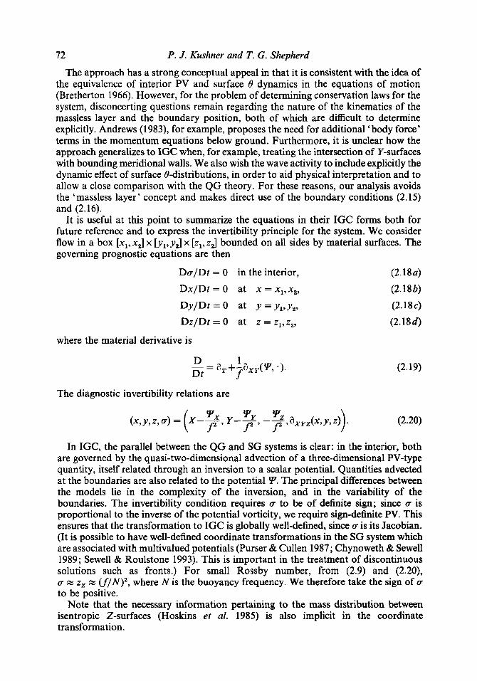
The approach has a strong conceptual appeal in that it is consistent with the idea of the equivalence of interior PV and surface 8 dynamics in the equations of motion (Bretherton 1966). However, for the problem of determining conservation laws for the system, disconcerting questions remain regarding the nature of the kinematics of the massless layer and the boundary position, both of which are difficult to determine explicitly. Andrews (1983), for example, proposes the need for additional ‘body force’ terms in the momentum equations below ground. Furthermore, it is unclear how the approach generalizes to IGC when, for example, treating the intersection of Y-surfaces with bounding meridional walls. We also wish the wave activity to include explicitly the dynamic effect of surface 8-distributions, in order to aid physical interpretation and to allow a close comparison with the QG theory. For these reasons, our analysis avoids the ‘massless layer’ concept and makes direct use of the boundary conditions (2.15) and (2.16).

It is useful at this point to summarize the equations in their IGC forms both for future reference and to express the invertibility principle for the system. We consider flow in a box [x,, x2] x [yl, y2] x [zl, zz] bounded on all sides by material surfaces. The governing prognostic equations are then

Dcr/Dt = 0 in the interior,

Dx/Dt = 0 at x = x,,x,,

Dz/Dt = 0 at z = z1,z2,

Dy/Dt = 0 at Y = Y ~ , Y Z ,

where the material derivative is

1 - = aT+-aXy(Y, .). Dt f D

The diagnostic invertibility relations are

( 2 . 1 8 ~ )

(2.18b)

(2 .18~)

(2.18d)

(2.19)

(2.20)

In IGC, the parallel between the QG and SG systems is clear: in the interior, both are governed by the quasi-two-dimensional advection of a three-dimensional PV-type quantity, itself related through an inversion to a scalar potential. Quantities advected at the boundaries are also related to the potential Y. The principal differences between the models lie in the complexity of the inversion, and in the variability of the boundaries. The invertibility condition requires n to be of definite sign; since n is proportional to the inverse of the potential vorticity, we require sign-definite PV. This ensures that the transformation to IGC is globally well-defined, since n is its Jacobian. (It is possible to have well-defined coordinate transformations in the SG system which are associated with multivalued potentials (Purser & Cullen 1987; Chynoweth & Sewell 1989; Sewell & Roulstone 1993). This is important in the treatment of discontinuous solutions such as fronts.) For small Rossby number, from (2.9) and (2.20), cr B zz x w / N ) , , where N is the buoyancy frequency. We therefore take the sign of cr to be positive.

Note that the necessary information pertaining to the mass distribution between isentropic Z-surfaces (Hoskins et al. 1985) is also implicit in the coordinate transformation.

Wave-activity conservation laws for semi-geostrophic dynamics. Part 1 73

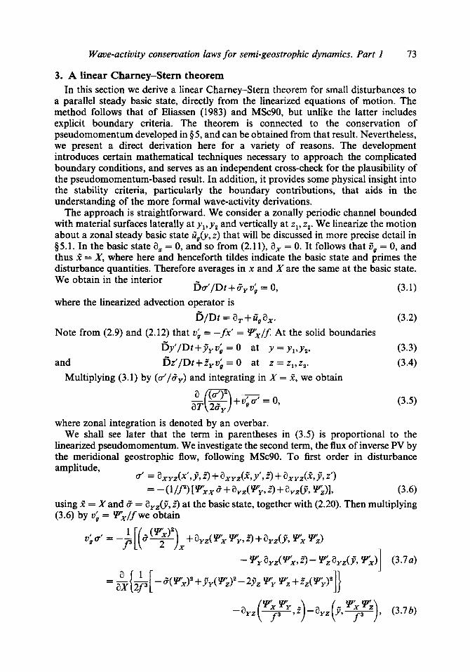
3. A linear Charney-Stern theorem In this section we derive a linear Charney-Stern theorem for small disturbances to

a parallel steady basic state, directly from the linearized equations of motion. The method follows that of Eliassen (1983) and MSc90, but unlike the latter includes explicit boundary criteria. The theorem is connected to the conservation of pseudomomentum developed in $ 5 , and can be obtained from that result. Nevertheless, we present a direct derivation here for a variety of reasons. The development introduces certain mathematical techniques necessary to approach the complicated boundary conditions, and serves as an independent cross-check for the plausibility of the pseudomomentum-based result. In addition, it provides some physical insight into the stability criteria, particularly the boundary contributions, that aids in the understanding of the more formal wave-activity derivations.

The approach is straightforward. We consider a zonally periodic channel bounded with material surfaces laterally at y, , y , and vertically at zl, z,. We linearize the motion about a zonal steady basic state ii,(y, z) that will be discussed in more precise detail in $5.1. In the basic state a, = 0, and so from (2.11), a, = 0. It follows that ijB = 0, and thus I = X, where here and henceforth tildes indicate the basic state and primes the disturbance quantities. Therefore averages in x and X are the same at the basic state. We obtain in the interior

where the linearized advection operator is

Note from (2.9) and (2.12) that vi = - fx’ = Vx/J At the solid boundaries

W / D t + Zy V ; = 0,

6 / D t = aT + fig a,.

(3.1)

(3.2)

and Multiplying (3.1) by (u’/ZY) and integrating in X = I, we obtain

where zonal integration is denoted by an overbar. We shall see later that the term in parentheses in (3.5) is proportional to the

linearized pseudomomentum. We investigate the second term, the flux of inverse PV by the meridional geostrophic flow, following MSc90. To first order in disturbance amplitude,

= - (w) t v;x 5 + a y z v y , .a + ayzv, vZ)i, (3.6) using I = X and Z = a,&, 5) at the basic state, together with (2.20). Then multiplying (3.6) by vi = !P&/fwe obtain

- ayz (F, 2) - ayz (y, y), (3.7b)

74 P . J . Kushner and T. G . Shepherd

where in (3.7b) we have used thermal wind balance to take i, = yZ (see (2.20)). Then invoking periodicity in X, we obtain

0; = a y z ( v ; y , + ayz(y, 0; z’). (3.8)

The expression (3.7b) is the linearized E-P flux divergence, as will be seen in $7, and as is noted by MSc90 for the compressible /3-plane case. Consider now the global integral of (3.8) over the domain in IGC:

where we have changed variables in the final step. The basic-state limits of integration in IGC are symbolized by B, while the limits of integration in physical coordinates are constant and the region is denoted D (cf. $5). Note that y’ and z’ are fluctuations in IGC and may be sensibly defined as functions of the physical coordinates. Now

a,,&% 0; y’, 3 = a&; v’) 12. p ,

and similarly for the second Jacobian in (3.9). Then (3.5) and (3.9) imply

which after using (3.3) and (3.4) may be written

where we have used the fact that in the basic state, averages in X and X are identical. Equation (3.10) and its generalization to the compressible /3-plane case (9.17)

provides a statement of the linearized Charney-Stern theorem for this system. If 52., throughout the interior, -JY over y = y,, y y over y,, -2, over z2, and 2, over z1 all have the same sign, then the disturbance may not grow (in a mean-square sense). Following MSc90, we can restate the result in terms of particle displacements 7’ brought about by the meridional geostrophic wind. Defining 7’ by

U; = fi>r’/Dt

we may integrate (3.1), (3.3) and (3.4) to obtain

I a’ + 5,q’ = 0 in the interior,

y’+.P,7’ = 0 at y = Y1,YZ,

z’+2,7’ = 0 at z = z1,z2,

(3.11)

so that we may rewrite (3.10) as

Equations (3.10) and (3.12) provide statements of ‘formal stability’ (Holm et al.


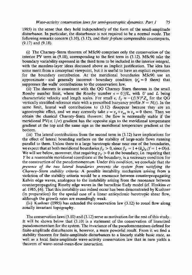
1985) in the sense that they hold independently of the form of the small-amplitude disturbance. In particular, the disturbance is not required to be a normal mode. The following remarks concern (3. lo), (3.12), and their P-plane compressible counterparts, (9.17) and (9.18).

(i) The Charney-Stern theorem of MSc90 comprises only the conservation of the interior PV term in (9.18), corresponding to the first term in (3.12). MSc90 take the boundary variability expressed in the third term to be included in the interior integral, with the massless-layer ideas discussed above as implicit justification. The idea has some merit from a conceptual viewpoint, but it is useful to have an explicit expression for the boundary contribution. At the meridional boundaries MSc90 use an approximate - and generally incorrect - boundary condition (vh = 0 there) that suppresses the walls’ contributions to the conservation law.

(ii) The theorem is consistent with the QG Charney-Stern theorem in the small Rossby number limit, where the Rossby number e = U/fL, with U and L being characteristic velocity and length scales. For small e, ,ZY z - ( f / N ) 2 Z y for the QG vertically stratified reference state with a prescribed buoyancy profile N = N(z). In the same limit, lateral wall contributions to (3.12) disappear because they are an ageostrophic effect, and we may correctly take u = vg+vag z ug = 0 there. Then we obtain the classical Charney-Stern theorem: the flow is necessarily stable if the meridional P V ( a l/g) gradient has the opposite sign to the meridional temperature gradient at the top and the same sign as the meridional temperature gradient at the bottom.

(iii) The lateral contributions from the second term in (3.12) have implications for the effect of lateral bounding surfaces on the stability of large-scale flows running parallel to them. Unless there is a large barotropic shear near one of the boundaries, we expect that at both meridional boundaries j jy > 0, since 9, = 1 + (QY/f = 1 + O(e). We will see below, moreover, that requiring y, > 0 at the boundary, i.e. requiring that Y be a reasonable meridional coordinate at the boundary, is a necessary condition for the construction of the pseudomomentum. Under this condition, we conclude that the presence of the two lateral boundaries prevents the system from satisfying the Charney-Stern stability criteria. A possible instability mechanism arising from a violation of the stability criteria would be a resonance between counterpropagating Kelvin edge waves, analogous to the instability arising from the resonance between counterpropagating Rossby edge waves in the baroclinic Eady model (cf. Hoskins et al. 1985,56). That this instability can indeed occur has been demonstrated by Kushner (in preparation) for the special case of a linear anticyclonic barotropic shear flow, although the growth rates are exceedingly weak.

(iv) Kushner (1995) has extended the conservation law (3.12) to zonal flow along zonally invariant topography.

The conservation laws (3.10) and (3.12) serve as motivation for the rest of this study. It will be shown below that (3.10) is a statement of the conservation of linearized pseudomomentum for the system. The invariance of the pseudomomentum defined for finite-amplitude disturbances is, however, a more powerful result. From it we find a stability theorem for finite-amplitude disturbances to a linearly stable basic state, as well as a local finite-amplitude wave-activity conservation law that in turn yields a theorem of wave-zonal-mean-flow interaction.

76 P. J . Kushner and T. G. Shepherd

4. Global invariants We consider closed box, channel, or doubly periodic boundary conditions. Working

with the system in physical coordinates, we obtain from (2.2)-(2.8) the energy flux law

is the energy density in (x,y,z)-space (Hoskins 1975). Under the Boussinesq approximation, variations in density do not contribute to the energy. The density is thus factored out of (4.2), so that the energy has dimensions of velocity squared. Integrating (4.1) over the domain using the boundary conditions (2.16) and either (2.15) or x or y periodicity, we obtain conservation of the total energy, I :

(4.3)

In a similar manner, (2.2a) can be rewritten as a local flux law for the zonal impulse M :

where

Mt + v, * (uM) + a,(wM) + $hZ = 0,

M = - f Y

has dimensions of momentum divided by mass. There is a corresponding conserved global impulse A for flow periodic in x:

With material conservation of u (2.18a) and of Z (2.7), we may determine a family of globally conserved quantities. For any function C(cr, Z ) we find using the continuity equation (2.6) that

This yields the global conservation law

(4.7) Ct+v,'(uC)+a,(wc) = 0.

In the variational calculations below we will use the IGC form of the fields. The functional variations will be taken on integrals over the field densities in IGC, i.e. the densities in physical space multiplied by the Jacobian of the transformation from physical coordinates to IGC, axuz(x, y, z ) = u. For example the zonal impulse density in IGC is M*, defined by

A = Mdxdydz = M*dXdYdZ, (4.9)

(4.10) s

M* = -flu. I

i.e.

The functionals V thus take the form

V = C*(CT, 2) dXd YdZ, (4.1 1) I where C* = aC(a,Z) is an arbitrary function of cr and Z.

The conservation of the quantities 8, A, and W is linked to the underlying Hamiltonian structure of the dynamics (Salmon 1985, 1 9 8 8 ~ ; Roulstone & Norbury


1994; Kushner 1993). From this point of view, d is the Hamiltonian functional reflecting, through Noether’s theorem, the time symmetry in the system, and A the corresponding zonal impulse invariant reflecting the system’s zonal symmetry. The functionals ‘2? are the system’s Casimir invariants, arising from degeneracies in the Poisson operator in the Hamiltonian formulation, and corresponding to the ‘particle relabelling’ symmetries (e.g. Salmon 1988 b ; Shepherd 1990). Further discussion is provided in Part 2 of this study (Kushner & Shepherd 1995).

5. Pseudomomentum A ‘wave-activity’ invariant is defined to be a conserved quantity that is second order

in the amplitude of a disturbance to a reference or ‘basic’ state with some continuous symmetry. A review of the concept of these invariants, together with a general discussion of their role within Hamiltonian theory, is provided by Shepherd (1 990). The ‘pseudomomentum’ is the wave activity, defined with respect to zonally symmetric basic states, that is associated with the zonal symmetry of the system; it is an exact invariant of the nonlinear dynamics. In a similar way the pseudoenergy, which is considered in Part 2 of this study, is associated with the temporal symmetry of the system and is likewise an exact invariant. The ‘wave action’ (Whitham 1965; Bretherton & Garrett 1968) is related but distinct from these quantities; it is associated with the symmetry properties of a phase-averaged Lagrangian, rather than an exact coordinate symmetry.

5.1. Basic state

Consider a steady zonal basic state in physical space. As noted in $3,a, = 0 implies that a, = 0 in the basic state. Because a, = $,.f = 0 in the basic state, the meridional boundaries are straight in IGC, i.e. constant in Y for all X , at every Z-level. However, in general the distance q- may vary with Z, and the bounding z-surfaces will be curved as well.

At the basic state (Y,4 = ( * ( y , z ) , e ( y , z ) ) . (5.1)

Following previous approaches (e.g. McIntyre & Shepherd 1987; S89) we define an inverse map in the interior, znt(e, 2) : for every Z, values of r~ map onto particular Y- values at the basic state. If e is not monotonic in Y, znt will be multivalued in e, and additional Lagrangian information will be needed to fully define the inverse map. See McIntyre & Shepherd (1987) for a more complete discussion of this issue.

At each of the surfaces at the basic state, there is an isentropic distribution zs( Y ) , where s is a discrete index specifying the surface. Let us denote the surface inverse map z ( Z ) such that for example at z1

g ( Z ) = [zz,( Y)]-l at the basic state, lower z-surface.

Depending on the monotonicity of 2 in Y, may also be multivalued. The index s serves in a sense as another Lagrangian marker. There is also a basic-state surface distribution of e, labelled eS, and defined by

3s(z) = 3( Q Z ) , Z ) . (5 .2 )

Although the surface maps are defined with respect to the basic-state Z-distributions, they may be treated simply as functions of 2 alone. Thus integrals over the functions are Casimirs of the form (4.1 l), although independent of r ~ . It is for this reason that 8, is defined as a function of Z rather than of Y.


(4 (6)

Z

z.

z. - - -

I I b

yc Y .

Y

FIGURE 1. (a) A zonal basic-state profile sketched in IGC. The heavy solid line shows the material boundaries, with the z = z1 surface unbounded to the south and ending at A to the north, the northern y = y , surface running between A and-B, and the upper z = z2 surface running south from B. The solid contours are curves of constant F(Y,Z) , a function monotonic in Y and Z . Dashed contours are of the surface function F,(Z). This basic state is linearly stable for -d, > 0. (b) As in (a), but for a basic state breaking the stability criteria in two ways, for -CY > 0: the presence of the southe-m boundary y = y l , between C and E, and a surface warm anomaly at Y = < on the z,-surface. Now e ( Z ) is multivalued.

Figures 1 (a) and 1 (b) illustrate the definition of the surface maps. Figure 1 (a) depicts a Y, 2 cross-section of a zonal basic state that would be stable according to (3.10) for positive interior PV gradients, - d , > 0. The flow is unbounded to the south, the lower boundary z = z1 ends at point A, the northern boundary y 2 runs between A and B, and the upper boundary z2 continues south from point B. For these boundaries -2, at zl, 2, at z2, and j y at y, are all positive for Zz > 0. Consider a function i( Y, Z ) which for purposes of this illustration is monotonic and increasing in both Y and 2. Contours of P are sketched in the figure. At a boundary, the surface distribution 4 is defined uniquely for all 2: we define it to be the value of at the point (Y , ,Z) where the surface’s isentropic height is 2. Horizontal contours of are sketched with dashed lines in the figure. Hence &Zi) = El(Zi) = 8 and E(ZJ = F,,(Zf) = 4.

Considering figure l (b) , we see how the uniqueness of the inverse surface maps is broken under conditions that violate the linear stability criteria. We include for illustration two ‘problem’ regions, a ‘bump’ (corresponding to a ‘warm anomaly’) at r, on the z,-surface, where 2, changes sign; and the presence of a southern boundary y = y1 with Y y > 0 running between points C and E. &Z) is no longer defined without additional ‘point of origin’ information. At Z j , for example, the function can take either the value 8 if s = y, or & if s = y,. At Zi, the function can have one of four values : 4 if s = y z ; 4 if the region Y > r, is specified on z1 ; F, for s = z1 and Y < ; or 4 for s = yl. We emphasize the connection between violation of the stability criteria and the multivaluedness of whatever the monotonicity properties of F.

5.2 . Fin ite-amplitude pseudomomen tum We seek a conserved quantity, 9, that is second order relative to the zonal basic state. This requires that Y be of the form

(5.3) Y = 4 4 - d [ 5 ] ,


FIGURE 2. Cross-section of boundaries for a given basic state (heavy solid curve ABCE) and perturbed state (lighter solid curve A'BC'E') at a given value of X . The hatched region is D'. The arrows at P and N represent positive and negative 2-variations of the 2,-surface. The cross-hatched region near the upper and northern edge B is of second order relative to the variations at P and N.

where (T and 2 symbolize all perturbed and basic-state fields, and that si2 be extremal at the basic state, i.e.

S d = 0 at the basic state. (5.4)

In order to apply a variational principle of the form (5.4) we must include the variation at the boundaries explicitly. Consider an integral 9 of a density F whose local variation is denoted SF. Rather than specify limits of integration, we will denote the variable region as 0" and variations to it by D'. We find

The variations at x1 and x, cancel owing to periodicity. The quantity 6 Z ) , is the displacement in IGC of the z1 boundary at a given ( X , Y), and SYI,, s(mi1arly represents displacements of y, in IGC for each ( 2 , X ) . These displacements are unambiguously defined as long as

0 < Iyy Jz,x I < 00 at y-boundaries, 0 < (zz I x , 1 < 00 at z-boundaries, (5.6)

for both the perturbed and unperturbed boundaries. If we take the gradients to be positive, the conditions (5.6) require, in essence, that Z and Y act as sensible vertical and meridional coordinates in a statically stable flow with Rossby number less than unity (see remark (iii) in $3).

We note that (5 .5 ) neglects as second-order quantities the variations in the limits of integration along the meridional edges {(x, y,, zl): x, < x < x,}, etc. The contributions at the corners cancel owing to periodicity. Hence, to leading order, the limits of integration on all the integrals are taken to be those of the basic state and there is no additional need to consider the variations D'. The subscripts 0" on the surface y- and z-integrals indicate this approximation.

Figure 2 schematically illustrates the boundary variations in IGC. At a given X, the


boundary of the domain is outlined by a heavy curve for the basic state and a lighter curve for the perturbed (non-zonal) state. The region D' is the hatched region representing the perturbation of the domain. A perturbation 6Z1,, is shown to be positive at point P and negative at point N. It is supposed that under perturbation, each point on a given bounding surface maps onto another, and the variations 6 Y I,, 6Z 1, parametrize these displacements everywhere except near the edges. Such a second-order edge contribution is represented by the cross-hatched region in the figure.

Consider, for example, variations in the zonal impulse A. From (4.9), (4.10) and (5.5),

jYa621,,dXdY . (5.7)

Clearly the zonal impulse is not extremal for this basic state as its first variation is, in general, non-zero. As is standard practice for wave-activity construction (e.g. Shepherd 1990), we define the invariant

d = .M+%, (5.8)

whose conservation is guaranteed by (4.6) and (4.8), and then determine %? such that d satisfies (5.4). On general grounds one may always expect such a '3 to exist (e.g. Shepherd 1990).

-[1,.6 11::

For any Casimir '3 of the form (4.1 I),

(5.9) In order to satisfy (5.4), we require from (5.7) and (5.9) that

X*/i3a Iz = jY in the interior, basic state, (5.10)

C* =flu at all boundaries, basic state.

A Casimir density satisfying (5.10) takes the local form

C*(a, Z ) = fin&+, Z) d++fls(Z) c?#(Z). (5.11)

We now consider a finite-amplitude disturbance to the basic state. We define

Y = *+ Y , rJ = 8+d, (5.12)

where we have dropped the &variational notation to emphasize that the disturbance can be large. We leave the limits of integration of both the 6- and the D'-regions unspecified for the moment.

and ZS are only defined over the range of values of cr and Z present in the basic state. If the disturbance (5.12) introduces values outside that range, then the function (5.1 1) must be extended to include such values. One can make this extension arbitrarily without compromising the fact that C* is a Casimir

r *,(Z)

disturbance quantities !P' and a' by

Note that the inverse maps xnt,

Wave-activity conservation laws for semi-geostrophic dynamics. Part I 8 1

density, and is therefore conserved (cf. Arnol'd 1966). Bearing this possibility in mind, the finite-amplitude pseudomomentum can be written

9 = A[u]+%[cr]-A[8]-%[8]

g,,(&,Z)d&+ E(Z)e , (Z) dXdYdZ 1 cnt(&, Z) d& + t ( Z ) 8,(Z)

[E,,(&,Z)- znt(8,Z)]d& dXdYdZ 1 + ID [ l, grit(+, Z) d& - Y8 + E ( Z ) C,(Z)

[E,,(8+&,Z)- Ent(8,Z)]d& dXdYdZ 1

= Yint + Y,,

where in the derivation of (5.13) we have used the identities

Z,t@, 2) = Y, g , m Z ) , Z) = QZ).

(5.13)

The final expressions in (5.13) formally define the pseudomomentum in terms of both surface and interior contributions.

5.3. Comparison with QG theory and small-amplitude reduction It is worthwhile to compare (5.13) with the pseudomomentum invariant of QG theory. From S89,

+i (-1 (-1)'l z, P f g [ ~ [ ~ i ( 8 + d ) - ~ i ( 8 ) ] d d N " 6 1 dxdy. (5.14)

In (5.14), p = p(z), 8# = 8,(z) and N = N(z) are the prescribed reference-state density, potential temperature and buoyancy frequency profiles, q is the QG PV, and 8 = 8+ 8' the potential temperature deviation away from 8,. Both q and 8 are related, via the QG invertibility principle, to the stream function. The form, as written, is defined on the 8-plane, with the 8-term included in the definition of the PV. The Znt maps defined at every height z are similar to those we have used for the SG analysis except that there is no explicit interior-surface connection as defined in (5.2). The reason for this is that z is not a dynamical variable in the QG model.

82

(5.13) and (5.14), are analogous. At small amplitude

P. J . Kushner and T. G. Shepherd

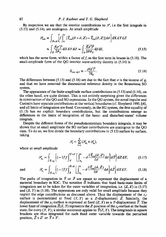
By inspection we see that the interior contributions to 9, i.e the first integrals in

q,, = s [fl[ Znt(3 + 6, Z) - gnt(5, Z)] d 6 dX d Y dZ d+D 1

(5.15)

which has the same form, within a factor off, as the first term in braces in (3.10). The small-amplitude form of the QG interior wave-activity density in (5.14) is

(5.16)

The differences between (5.15) and (5.16) are due to the fact that Q is the inverse of q, and that we have removed the dimensional reference density in the Boussinesq SG system.

The appearance of the finite-amplitude surface contributions in (5.13) and (5.14), on the other hand, are quite distinct. This is not entirely surprising given the differences in construction of the QG and SG expressions. In the QG system, the zonal impulse and Casimirs have separate contributions at the vertical boundaries (cf. Shepherd 1990, §4), and all limits of integration are fixed. Conversely, in the SG system, the first equality of (5.13) has no explicit boundary contributions, but the contributions emerge as differences in the limits of integration of the basic- and disturbed-states' volume integrals.

Despite the different forms of the pseudomomentum boundary integrals, it may be shown that at small amplitude the SG surface contributions are analogous to the QG ones. To do so, we first divide the boundary contributions in (5.13) surface by surface, taking

2 x = c (%{+%J i=l

where at small amplitude

The paths of integration in E or 2 are meant to represent the displacement of a material boundary in IGC. The notation 0" indicates that fixed basic-state limits of integration are to be taken for the outer variables of integration, i.e. (Z, X) in (5.17) and (X, Y) in (5.18). The expressions are only valid for small amplitude because they neglect the edge contributions as discussed above. Thus the displacement of the zt- surface is parametrized at fixed (X, Y) as a Z-displacement 2. Similarly, the displacement of the y,-surface is expressed at fixed (2, X) as a Y-displacement f. The lower limit of integration 2 ( X , Y) represents the 2-position of the z,-surface at the basic state, for every (1, Y); a similar statement applies to P(Z, X). The integrands in square brackets are thus integrated for each fixed outer variable towards the perturbed position, Z + Z or P+ Y.


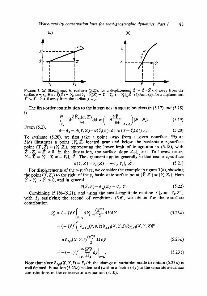
FIGURE 3. (a) Sketch_ used to evaluate c5.2?), for a displacemen! 2’ = 2-2 < 0 away from the sprfae-z =,zz. Here Y,(Z) = &, and Y, - Y,(Z) = - & x - Y, Iz2 Z’ . (b) As in (a), for a displacement Y’ = Y - Y > 0 away from the surface y = y , .

The first-order contribution to the integrands in square brackets in (5.17) and (5.18) is s:, -u a $mi(‘, a‘ ‘) d s x ( -cr- -a2qJ6-68).

6-+., = 6 ( Y , Z ) - 6 ( ~ ( Z ) , Z ) x ( Y - K(Z))6.,.

(5.19)

(5.20) From (5.2),

To evaluate (5.20), we first take a point away from a given z-surface. Figure 3 (a) illustrates a point (5, a located near and below the basic-state z,-surface point (5 , a = (5, ZJ, representing the lower limit of integration in (5.18), with 2-5 = 2 < 0. In the illustration, the surface slope Zyl z , > 0. To lowest order, Y- Y, = 5 - yZ x - Yz I z e 2. The argument applies generally so that near a 2,-surface

5( Y, Z ) - +,((Z) = - cy Y, I Z ( 2. (5.21)

For displacements of the y-surface, we consider the example in figure 3 (b), showing the point (9, Z,) to the right of the y, basic-state surface point ( y, Z,) = (Y,, Z,). Here ?-

6( f, Z ) - 6Yy,(z) = 6, 2. (5.22)

Combining (5.18)-(5.21), and using the small-amplitude relation z’ Iz = - Z Z Z 1, with Zz satisfying the second of conditions (5.6), we obtain for the z-surface contribution

= ?‘ > 0, and in general

(5.23~)

(5.23~)

Note that since az&, Y, Z) = Zz/+, the change of variables made to obtain (5.23b) is well defined. Equation (5.23 c) is identical (within a factor off) to the separate z-surface contributions in the conservation equation (3. lo).

84

from (5.14),

P . J . Kushner and T. G . Shepherd

The QG contribution to the wave activity at small amplitude at the z-surfaces is,

(5.24)

with fluctuations defined in the physical coordinates. The form (5.24), representing the boundary available potential energy, is analogous to (5.23 c) after appropriate scalings of the fluctuations and gradients.

Similarly to the derivation of (5.23) it may also be shown that

whose form is identical within the f-factor to the meridional boundary contributions in (3.10). In deriving (5.25) we have used the relation y' J y = -yy Y' l v , requiring that jy satisfy the first of conditions (5.6). As noted in $3, the contributions from the lateral boundary have no counterpart in QG dynamics, in which the standard scaling sets the normal component of the geostrophic velocity to zero on the boundary.

From (5.15), (5.23) and (5 .25) , we conclude that within a factor off, 9' reduces at small amplitude to the quantity in braces in (3. lo).

6. Nonlinear stability The stability analysis presented here follows the approach of S89. In 55.3 we have

shown that the sign of the small-amplitude form of the pseudomomentum (5.13) depends entirely on the signs of the meridional gradients of basic-state quantities. By conservation of the pseudomomentum these sign-dependences define a linearly stable basic state. It turns out that it is possible to define a positive-definite measure of the disturbance that is bounded for finite-amplitude disturbances to such basic states. Unlike the QG case of S89, however, the nonlinear stability theorem presented here only applies to a restricted class of perturbations, and the disturbance quantity is not, in general, a norm.

S89's approach is to bound a disturbance enstrophy-like norm from above and below by the QG pseudomomentum. Then using pseudomomentum conservation, the norm may be bounded in terms of its initial value, which is a statement of Liapunov stability. The method is first illustrated here for the simple case of a disturbance to a zonal basic state under the restriction that the disturbance vanish on the boundaries. Alternatively, the domain might be periodic or unbounded in x and y , and bounded vertically by isentropic surfaces. The boundary contributions represented by the integration over D' in (5.13) then vanish. For small-amplitude stability ZY must be sign-definite in the interior, and for definiteness we choose it to be negative with a view to the meteorological case. We suppose further that there exist functions K,(Z) and k,(Z) such that in the interior

(6- 1) 0 < k,(Z) < - 3y < K,(Z) < CO.

At every point (A', Y , Z ) in the interior

where Sint is the interior wave-activity density, defined as the quantity within square brackets in (5.15).


In this case we may define a disturbance norm llcrlll by

and we find ~ ~ ~ ’ ~ ~ z ( t ) < -y(t) = - y (o ) < Mllg’112(0)7 (6.4)

where M = max ( K J k J . (6.5) Z

We have used pseudomomentum conservation in (6.4). The maximum in (6.5) is taken over all Z-levels in the interior.

The inequality (6.4) is a statement of Liapunov stability similar in form to the QG case of S89, without the z-boundary contributions. A potential tightening of the bound relative to the approach of that study has been realized by considering the (- 3y)max/( - 3y)min ratio at each level and seeking its maximum, rather than taking the ratio of the global maximum and minimum values. This modified approach follows Held’s suggested improvement to the saturation bound of the two-layer model in Shepherd (1988) (see $5 of that paper).

We now proceed to construct a Liapunov stability theorem explicitly including boundary contributions. In order to do so we have found it necessary to consider a restricted class of perturbations, namely those that vanish along the edges of the domain. The edges are the four lines defined by {(x, y , , z,): x E [xl , XJ}, etc. Restricting the perturbations in this way makes the expressions (5.17) and (5.18) exact at finite amplitude: we may think of the displacement of the surfaces in IGC as that of a membrane fixed at its boundaries, like a drum. The restriction is artificial but appears necessary to obtain the nonlinear stability theorem.

A second problem emerges when considering the potentially destabilizing role of the meridional boundaries. From $3, remark (iii), we recall that Yuy, and Yy, will have opposite sign, at least at small amplitude. The point is also clearly illustrated by (5.25), where we see that for 3 > 0 at the boundaries, the northern contribution must be negative and the southern one positive. A basic state that satisfies the Charney-Stern stability criteria, then, cannot be constructed if variability is allowed at all bounding surfaces. Thus, besides the edge restrictions, we further take the perturbations to vanish at lateral boundaries, in which case yU, = 0. We expect the bounds to apply to regimes where the disturbance region is located well away from lateral boundaries. It is important to remember that the necessity of considering these restrictions for the nonlinear theory does not invalidate the linear stability theorem of $3.

Without a detailed knowledge of the particular basic state to be considered it is difficult to determine the tightest bound on the complex expression (5.18); thus we just provide a general bound that might be tightened for a specific basic state. We suppose that the basic state obeys (6.1) both in the interior and, in addition, at the boundaries. For linear stability, -z”y at the lower surface and ZY at the upper surface were required to be positive. For nonlinear stability, we further require that the quantities

- ( - V Y Z I Z , = (-l>i(zz/zY)lzt

and 3 are positive and bounded away from zero and infinity at the boundaries. We bound the surface wave-activity densities Sz, (defined as the double integrals

within braces in (5.18)) as follows. For example, the lower surface contribution obeys

86

where kzi is defined generally by


[ - (- l)i (Y, I,)]]. (6.7) 1

The maximum in cr in (6.7) is taken for c r ~ [ 6 ~ ~ . G ] ~ and that in 2 taken for ZE [p, 3 + 2’1. We may also define the positive functions

[ - (- l)i (Y, I,,)]]. (6.8)

Therefore

Following the same approach as the derivation of (6.4), we define a positive-definite measure of disturbance amplitude by

(6.10)

Because the limits of integration of the first integral of (6.10) depend on Z’, Ilcr’II does not satisfy the homogeneity property Ilhcr’II = lhl IIdII, where h is a constant and (T’

represents the vector of disturbance quantities (g’, 2’ I,,>. Thus (6.10) does not qualify as a norm. Nonetheless, the expression may be bounded from above and below in the same way as (6.3) and may be shown to obey

l l ~ ’ I l Z ( ~ ) G Mllfl’1I2(0)Y (6.11)

with (6.12)

where the maximum over 2 is taken for all interior values of Z , and that over each z- surface taken for all (X, Y ) there. This proves nonlinear stability.

The bound (6.1 1) with (6.12) is analogous to the QG form found in S89, which also consisted of interior and vertical boundary terms. The differences lie in the restrictions on the perturbations, and in the comparatively complex form of the quantities Kzt and k*,*

7. Local conservation law We now develop a local wave-activity conservation law of the form

(7.1) r + V . F = O asin,

for the pseudomomentum density. Since (7.1) is a local relation, we can analyse the interior equation alone. Taking (7.1) as a definition of Fdoes not specify it completely: the field is only defined to within a non-divergent flux. To further specify the field’s form, we require that it satisfy the group-velocity property that in the WKB limit of a small-amplitude monochromatic wave packet propagating through a slowly varying medium,

where cg is the group velocity and the angular brackets denote a phase average.

(F) = Cff(SiRt)’ (7.2)


Consider the form of the interior pseudomomentum density Sint, the quantity within square brackets in (5.19, whose spatial integral comprises the interior contribution to the pseudomomentum (5.13). We note that from g-conservation (2.18a)

Now

whence

D6 D d - !P’’ I - Dt Dt f uy’

(7.3)

(7.4)

as,,, = f [ En,@ + u’, Z ) - ~, , (6 , Z ) ] ,

aqflt vf, es,,, = f [ Zfl,(6 + d, Z ) - E,,(6, Z ) ] - f -

a g

- a r 23

- Y&uf = -fv;u’. --(---)--- DS,,, - as,,, as,,, DZ

Dt au a d Dt (7.5)

Note that to within a factor off, the zonal average of (7.5) reduces to (3.5) in the small-amplitude limit, with the small-amplitude form of the density Sin, given in the IGC integral in (5.15). To obtain a finite-amplitude flux law, we must express fvh u’ as the divergence of a flux. This is done in Appendix A, gA.1, yielding a wave-activity conservation law of the form (7.1). In QG theory, the invertibility principle is linear, implying that the meridional PV flux has only quadratic terms at finite amplitude. From Appendix A, gA.1 we see that since the SG invertibility principle is cubic- nonlinear in Y, the finite-amplitude flux has terms of cubic and quartic order. The small-amplitude reduction of the flux is, from (A 3),

(7 * 6) iig s , , , - ; fY(v;)”;~[zz(y’)2-21y y’z’+yy(z’)y

f (Iz v; y’ - yz v;, z’)

f ( - I , v; y’ + y y v; z’)

The zonal average of V - F reduces to f times (3.8).

property, we introduce the WKB ansatz To explore the wave properties of the system, and to verify the group-velocity

!P’ = Re[Y*(~LX,~Y,’Z)e“K’X-”T’ I , (7.7)

where perturbation lengthscale a 1, ’ = wave envelope lengthscale

the dimensional wave vector K = (K, L, M ) , and Q(K, Y, 2) is the frequency. Substituting (7.7) into (7.6) and keeping the leading-order contribution in (u yields

(7.8) - ( -Ty KL +Y”,KM)

To verify the group-velocity property we must use (3.6), the linearized invertibility relation for small-amplitude disturbances to the basic state. From (3.6), in matrix form

= h,, ax( ax, Y , (7.9)

88

where

P. J . Kushner and T. G. Shepherd

(7.10)

is a symmetric matrix from the thermal wind relation. In order for (7.9) to be invertible, we require hij to be sign definite. We find

det ( -htj) = -, (V (7.1 1) 6

-h --, det f” l1 -f” implying that hi, is negative definite for a statically stable basic state (2, > 0) with positive PV. Substituting the WKB form (7.7) into (7.9) yields, to lowest order in p,

u ’ = - ~ ~ , K , K , ’ Y ’ . (7.12)

The dispersion relation obtains upon substituting the solution into the linearized governing equation and taking the terms of lowest order in p. We find

(7.13)

where the minus sign accompanies the denominator to keep the quadratic form positive. This is clearly analogous to the QG dispersion relation, which under the WKB approximation is

(7.14)

where w is the frequency, (k,I,m) the wave vector in physical space, and c&, is the meridional QG PV gradient. The group velocity is

where we have used the symmetry of hi*. The phase-averaged linearized pseudomomentum is, from (5.15) and (7.12),

(7.16)

and the group-velocity property (7.2) follows directly from (7.15) and (7.16) if we rewrite (7.8) as

(4,)) = (ti,(siat> -&j Ki Kj I P Iz) St,+ iKhlj Kj I ‘y*12* (7.17)

8. Wave-mean-flow interaction theory Using the results of $7 we develop diagnostic equations to determine the effects of

departures from the zonal flow on the zonal flow itself. We must first distinguish the time-dependent zonal-mean state e, from the steady zonal basic state G, with respect to which the disturbance cr’ is defined (see (5.12)). We may divide u‘ and the other disturbance fields into zonal and eddy parts as follows:

cr‘ = 7( Y, Z , T ) + cr*(X, Y, 2, T), such that 2 = 0. (8.1)


For small-amplitude disturbances, both 7 and cr* are small compared to 3. Using this decomposition based on the zonal-mean statistics of the flow we will be able to see clearly how the evolution of the zonal mean is influenced by a given eddy forcing.

We add a term G to the right-hand side of (7.1) to represent processes that generate or dissipate pseudomomentum locally. Then from the interior governing equation (2.18 a), (7.1) and (7.5), we find that to lowest order in the amplitude of the disturbance

We will examine (8.2) in some detail. The equation expresses the way in which eddies force the zonal mean cr (inverse PV) tendency. The components of the generalized E-P flux F are, from (7.6),

To obtain the QG limit, one may use the invertibility relations (2.20) to find

u”, x 1, iz x -, f y’ x -ug, 1 , z’ x - & Z x -- gB’ P f we,’

whence

where we have taken uh Iz % uh J E . The form (8.4) is a scaled version of the E-P flux from Edmon et al. (1980), with an overall change of sign due to their definition of the linearized wave activity, which is negative relative to (5.16).

Comparison of (8.3) and (8.4) suggests that the off-diagonal thermal-wind terms in the matrix play an important role in Rossby-wave propagation for large Rossby number. This can be seen from the meridional and vertical components of the group velocity (7.13,

where the thermal-wind terms affect the relative magnitudes of the horizontal and vertical components. Since both the basic-state and perturbation quantities depend on the coordinate transformation, however, the extent to which SG dynamics modifies the QG-dynamics-based picture of Rossby-wave propagation is not yet clear. This issue is currently being examined.

The relation (8.2) provides additional diagnostic insight when it is expressed as a wave-mean-flow closure. The idea, as in QG theory (see e.g. Andrews, Holton & Leovy 1987), is to determine the balanced zonal-mean response to a given eddy forcing. We will see, however, that the QG and SG forms of the zonal-mean balance differ significantly. The source of this difference lies in the nonlinear invertibility relation of SG theory, and can be seen by considering the zonal mean invertibility problem. In QG dynamics, q = Yo,(!?‘), where YQG is a linear operator and !P may be obtained from q subject to linear boundary conditions. The linearity of the system implies that the zonal mean - disturbance, - F, or the zonal-mean tendency u, = may be obtained given q’ or qk. The SG invertibility relation (2.20), on the other hand, may be represented symbolically by u = JV( Y, Y, 9. Since the system is invertible by assumption, !P may be obtained from n, but a closure problem emerges when zonal-


mean quantities are desired, because 7 = -K( !P', Y* Y*, Y* Y* Y*, . . . ), i.e. correlations between eddy quantities come into play in the balance. Thus more than the 7 or distribution is needed to determine the corresponding

We find that the second-order eddy correlations are significant even in the linear theory. Equation (8.2) shows that the zonal-mean PV tendency (.;. is second order in disturbance amplitude a. In other words, the dynamics constrain the zonal-mean PV to evolve on a slow timescale. Thus, if 7 = 0 initially, we have 7/c? = @a2). From (2.20) we find to lowest order in disturbance amplitude that

or F.

7 = 9(F)+V. (8.6)

(8.7)

(8.8) In (8.6), we have neglected higher-order terms such as C?,,(y', z') and axyz(x*,y*, z*).

The zonal-mean stream-function tendency, K, can be obtained from the following :

where the linear operator 9 has the form

9 = -f-2 [FA * ) I T - 2Yz( .)YZ +YY( .)zzl,

v * J = axyZ(x*, y*, 5) + C?yz(y*, z*) + c:xuz(x*, 7, z*).

and the divergence term consists of second-order eddy correlations :

_ _

__ 2 a - q Y ; ) = --v. J=--v;a*

i3T c?Y (8.9a)

where we have used (8.2) and (8.6). The boundary conditions on ( 2 . 1 8 ~ d) , (2.20), and (3.3) and (3.4),

are, from

The quantities in square brackets on the right-hand sides of (8.10) are the scaled small- amplitude surface pseudomomentum densities in (3.10) (see also (5.23) and (5.25)).

The operator 9 is elliptic for a statically stable (Fz > 0) basic state with 6 > 0. The ellipticity is used in Appendix B to show that the solution %( Y, 2, T ) to (8.9) with boundary conditions (8. lo), for given -___ interior PV fluxfu; cr* = V - F, eddy correlations (V - JjT, and boundary fluxes (vQ y*, u t z*), is unique to within a spatially constant function of time. Since the Y-derivative of such a constant vanishes, and because this solution is unique, we obtain as a consequence the following non-acceleration theorem : in the absence of transience (namely (V - 4, = [SintlT = Z_guJ, = [sz,lT = 0), and of pseudomomentum generation and dissipation - (namely G = 0), the zonally averaged flow does not accelerate, i.e.

We may cast (8.9) into a form that allows us to obtain the zonal acceleration directly from the inversion. If an assumption is made that the basic-state meridional lengthscales are much larger than those of the disturbance, then -up' 9[c])y x 9(%), and we obtain

= u& = 0 throughout the domain.


Equation (8.1 1) closely resembles the wave-mean-flow balance of QG theory. In the QG limit, using scaling arguments similar to those used to derive (8.4), (8.11) becomes

(8.12)

Equation (8.12) matches the Boussinesq inviscid limit of equation (3.5.7) of Andrews et al. (1987), which expresses the QG zonal-mean response to eddy forcing in log- pressure coordinates. In deriving (8.12), we have neglected the term involving (V - & as being O(s) compared to the right-hand side of the equation.

In conclusion, we have shown that while PV fluxes suffice to determine the zonal- mean PV tendency (equation (8.2)), the nonlinearity of the invertibility relation implies that the zonal-mean stream-function tendency can only be obtained if the flux divergence tendency V is also specified. It is not obvious what net effect the eddy fluxes Jhave on the mean flow. As a limiting case, we find for WKB conditions (7.7) that they have no effect, since ((V - 3,) = 0.

9. P-plane compressible flow 9.1. Introduction

In this section, we extend the results of &j2-8 to the P-plane compressible system of MSc90. Like the Hoskins (1975) system, the MSc90 model has the same two mathematical features that made it possible to find the pseudomomentum in $5: first, its dynamics are also governed by PV advection, with appropriate boundary conditions, and an invertibility principle relating the PV and boundary terms to the velocity; and secondly, it is a Hamiltonian system. The explicit form of the Hamiltonian structure is presented in the sequel to this paper (Kushner & Shepherd 1995).

Given the similarity in structure of the two systems, many of the derivations of the results of this section closely parallel those of the previous sections. We will thus omit the details of the developments below, referring the reader to the earlier sections.

9.2. Semi-geostrophic dynamics for /?-plane compressible Bow MSc90 generalize the hydrostatic compressible equations to the /?-plane as follows :

Du,/Dt- M Y ) +PAVV,l = - U/P) P,, 1 DuglDt + M Y ) 24 +PAP,] = - (l/P)Pv. j (9.1)

where Ay = y - Y, f = f ( Y ) is the variable Coriolis parameter, and /3 = df/dY is constant. The coordinates are (x ,y,z) , where in contrast to the previous sections z refers to geometric height, not pseudoheight. Equations (9.1) anticipate the transformation to IGC by explicit inclusion of the coordinate Y in the variablefand in the Ay-terms. The terms in square brackets in (9.1) represent the SG approximation to the Coriolis terms f.2 x u in the horizontal momentum equations. These expressions do not represent the /?-plane approximation per se, since while /? is constant f still varies in Y ; nor is Ay a deviation from some reference latitude. Rather (9.1) to order Rossby number 6 accuracy expresses the behaviour of the geostrophic coordinate transformation on the /?-plane. MSc90 arrive at the equations by requiring that the horizontal advection in IGC space have the canonical form found in the first two components of (9.10) below. The ‘primitive’ momentum equations then follow on transformation back to physical space. Equations (9.1) are part of a family of results (e.g. Magnusdottir & Schubert 1991; Lu 1993) based on a similar approach of taking

92 P . J . Kushner and T . G . Shepherd

the advection to be simplified in the transformed coordinate space. Craig (1993) has shown that this form of the momentum equations also follows from a systematic asymptotic expansion of the primitive equations in a modified Rossby number.

The material derivative is (2.3), with velocity components given by (2.4), where here and henceforth z is taken to be the geometric height. The geostrophic velocity is now

where p is the density, the continuity equation

the thermodynamic equation

DO O

and hydrostatic balance requires ap/az = - g p .

We transform the system to IGC

(9.4)

(9.5)

(9.6)

where henceforth f =f ly ) , and because fvaries we choose not to rescale 0 as in (2.9). The Montgomery-Bernoulli potential (M* in MSc90) in IGC takes the form

(9.7) with Ii' = c,(p/p,>" the Exner function, and # = gz. Equations (2.10) and (9.7) differ only in their internal energy terms, which turn out to be closely related. Using (2.1), (2.9), and the ideal gas equation of state, it may be shown that c p T = -f2Z(z,-za), where z p is the pseudoheight, z , = HJK z 28 km the maximum of z p for standard atmospheric values (Hoskins & Bretherton 1972), and f is the constant reference value in (2.9). The sum of the first two terms in (9.7) is once again the Montgomery potential, and that of the first and third terms the geostrophic-coordinate potential.

1 ( v , f U

( X , Y , O , T ) = x + Q , y - - 8 , O , t ,

Y = #+c, r+;(u;+v; ) = #+sn+;(u;+v;),

The partial derivatives transform as

From (9.2) and (9.5H9.8) we find (MSc90)

yT = P t / P , y e = 1 7 9

with f = f l y ) . In IGC, the material derivative is

DX D Y DO - = aT+-a,+-ay+-ae, D Dt Dt Dt Dt


and using the momentum equations (9.1), the thermodynamic equation (9.4), (9.6) and (9.9), we find

(9.10) f ’ f

The material derivative in IGC is then

1 - = aT+-axy(p, .). Dt f D

(9.11)

Following MSc90 we introduce the potential pseudodensity u = f / q ( u * / g in their notation), where q is the dimensional potential vorticity. The PV is conserved following the motion, so that

D ( u / f ) / D t = 0.

The discussion of the boundary conditions in $2 applies here as well. Material boundaries obey the ‘no normal flow’ condition, equations (2.15) and (2.16). Note that because z is now a geometric coordinate, the second of these equations applies at geopotential rather than isobaric surfaces.

From MSc90, equation (4.1), we find

fl = - axY& YI p ) / g . (9.12)

To obtain an explicit invertibility principle, and to develop expressions for the local pseudomomentum flux below, it is necessary to relate the physical coordinates (x, y ) and the pressure p to the potential Y. The zonal coordinate x is easily obtained from (9.9a). For the meridional coordinate, the first component of (9.10) may be written as an equation quadratic in ug,

Yy = - f i g + (B/f) (24; + V i ) . (9.13)

We use a scaling consistency argument to determine the appropriate root to solve for ug =fey- Y). The quadratic terms in (9.13) are small relative to the linear term, for

where U and L characterize zonal and meridional velocity and length scales, E is the Rossby number, and ro the Earth’s radius. Thus even for planetary-scale waves we may reasonably take Ocfu,) = O(Yy), forcing a choice of the smaller root of (9.13), namely

(9.14)

because the larger root yields O(ug) = O ( y / P ) - lo3 m s-’. We have thus expressed y in terms of Y, Y, and Yy, and note that the relation is nonlinear.

ug = cf”/2P) [1 - (1 - 4Pf3(Pf-3(~x>2 - !4)>”21 = - yY/f+Pf4[(yx>2 + ( y Y ) 2 1 + “e/r,)2U1,

For the pressure, from the definition of the Exner function we have

P = PO(%/C,)”“ = P(Yd To summarize, the governing prognostic equations are

D ( u / f ) / D t = 0 in the interior, D x / D t = 0 at x = x , ,x , ,

D y / D t = 0 at Y = Y , , Y , , D z / D t = 0 at z = z1,z2,

(9.1 5 a)

(9.156) (9.1 5 c )

(9.1 5 d )

94 P. J . Kushner and T. G. Shepherd

with the material derivative given by (9.11). The diagnostic invertibility relations are

(9.16)

We note the additional nonlinearity for y andp in (9.16) as compared to thef-plane case (2.20). MSc90 characterize the nonlinearity as 'weak' in the sense that to good approximation the quadratic terms in, for example, (9.13) are small compared to the linear term, so that ug = - Yy/f( Y ) . Under a quasi-Boussinesq approximation, the pressure may be taken to be linear in Ye.

Simpler systems may be obtained from (9.15) and (9.16). For modelling on the$ plane, these equations may be used with f constant and p = 0. For modelling Boussinesq p-plane flow, equations (2.2) may be used with the terms f v and f u replaced by the terms in brackets in (9.1).

9.3. Linear Charney-Stern theorem Using the same direct methods of $3, we find that the linear Charney-Stern theorem takes the form

or in terms of the meridional geostrophic displacements r',

Here meridional gradients in 3 / f= l/q" replace those of 5 in (3.10). Sincefis variable, the effects of differential rotation are allowed for. The conservation of the first term alone corresponds to (5.9) of MSc90. We refer to the remarks following (3.12) for a discussion of the implications of the boundary terms.

9.4. Global invariants Considering the same flow domains as in 54, we obtain the energy flux law

E,+V,.[u(E+p)]+a,[w(E+p>] = 0, (9.19)

where E = p(+($ + v:) + @Ye + $ ) - p (9.20)

is the dimensional energy density in physical space. Integrating (9.19) over the domain using the boundary conditions (9.15 kf), or periodicity or unboundedness in some direction, we find conservation of d as given by (4.3).

The zonal impulse obeys

where

with

iwt + v,. (UM) + a,(wM) +p, = 0,

M = -pF( Y ) ,

dF/d Y =A Y ) .

(9.21)

(9.22)

(9.23)

For flow periodic in x, we have the corresponding global conservation law (4.6).


For any function C(u/f, 0) we have

@c), + v,. (WC) + a , ( w m = 0,

which implies the global conservation law for the Casimirs

(9.24)

?.!! dt = AjpCdxdydz dt = 0. (9.25)

For the variational calculations we will again need the IGC form of the fields. The IGC zonal impulse density M* is

M * = - F ( Y ) u * A = M*dXdYd@, (9.26)

where we have used the relation paxue(x,y,z) = u, which follows from the fifth component of (9.16) together with hydrostatic balance (9.5). The functionals %' have the form

%? = fC*(a/f , @)dXdYdO, (9.27)

I

I where C* is an arbitrary function of two arguments.

9.5. Pseudomomentum The basic state is given by (5.1), and we will make use of the inverse maps

E,,<../f, 0) = F( G , , ( a @))?

where F is defined by (9.23), and the boundary maps E(0) = F( E.0)) and [@/A, (0). We seek 9 of the form (5.3), involving the sum of the zonal impulse and a Casimir chosen to satisfy the extremal property (5.4). Boundary variability is treated similarly to thef-plane system. From (9.26) and (9.27), (5.10) is replaced by

} (9.28) aC*/a(u/f) = F( Y) in the interior, basic state,

C* = F(Y)(a/f) at all boundaries, basic state, with solution

C*(v/ f , 0) = E n t ( G / f , 0) d(G/f) + E(0) [3/fl, (0). (9.29)

Using disturbance quantities as defined in (5.12), the /?-plane compressible version

[5/fI,(e)

of (5.13) is then

= x,, +s$. (9.30)

Following the approach of 9 5.3, the small-amplitude reduction of the pseudomomentum (9.30) yields the quantity within braces in (9.17). Note from (9.23) that for f > 0, F is monotonic and increasing in Y, and thus the ent and Ent maps play analogous roles in the stability theory.

96 P. J . Kushner and T. G . Shepherd

9.6. Stability The nonlinear stability theorem has the form (6.11) and (6.12) with the following substitutions : - -

u -+ (u/f) , Z + 8, Knt + &t,

in (6.1), (6.7), (6.8), and (6.12); and with (6.10) replaced by

(9.31)

9.7. Local conservation law From (9.30) the interior pseudomomentum density and its small-amplitude reduction are

Similarly to the derivation of (7.3, we find

(9.33)

The term !Px u' is expressed as the divergence of a flux in Appendix A, gA.2. To do so it is necessary to expand y - and p-fields in powers of the disturbance field Iy', because from (9.16) y and p are not integer powers of gradients of Y. The small-amplitude reduction of the E-P flux is, from (A 5) and (A 12)

(9.34 b)

(9.344

where !=A1 +4/3!Py/f3)1'2, Y = dp/d!€'@ = p 0 . (9.35)

In deriving the above we have used the small-amplitude relation

Y' = q f = - W(fA, together with thermal wind balance in the basic state

(9.36)

f J e = - ~ y / ~ h , (9.37)

both of which may be found using (9.16). Using the WKB ansatz (7.7), with 2 replaced by 0,

(9.38b)

(9 .38~)


To verify the group-velocity property, we have from (9.16) that to leading order

CTf = hij ax< ax, Y +pi ax{ Y , (9.39)

The matrix hi, is symmetric from thermal wind balance (9.37). In order for (9.39) to be invertible, we require hi, to be sign definite. As in the Boussinesqf-plane case, for a statically stable basic state with positive PV, hi, is negative definite since in that case

I - f(+/f)Z - hll -h ---0, det = -Ma> 0, det (- h,) = - > 0. (9.41) CT

df l1 - f 2

Under the WKB approximation

CT’ = -hij Ki Kj Y , the dispersion relation is -

o = - y K + ( - h ( w 9 Y K K ) ? K i j i j

and the group velocity is

(9.42)

(9.43)

which follows from the symmetry of h,. The phase-averaged linearized pseudomomentum is, from (9.32) and (9.42),

(9.45)

and the group-velocity property follows directly from (9.44) and (9.45) if we rewrite (9.38) as

(9.46) 2

9.8. Wave-mean-flow interaction theory We find that (8.2) holds withfvariable and Sinl given by the small-amplitude form in (9.32). The zonally averaged E-P flux is given by

(9.47)

Equation (8.6) holds with the operator


where the subscripts 1 and 2 indicate the first- and second-order terms in the expansions of p' and y' in (A 4) and (A 7). The linear terms in the Jacobians in (9.49) are

x* = - P X / f 2 , y: = - %/( fyj, p : = f!P& (9.50)

and the zonally averaged quadratic eddy correlations are, to leading order,

(9.5 1)

The nonlinear relation between p , y and Y in (9.16) implies, bearing in mind the discussion of $8, that the boundary conditions on %will be more complex than (8.10).

Y;. = -K/(ffi+G (9.52) We find from (A 7) that -

and from (9.16) that

(9.53)

The boundary conditions on % are thus, from (9.15c, d) ,

(9.544

The ellipticity of the operator (9.48) is guaranteed for a statically stable positive-PV basic state. The proof of uniqueness of the boundary value problem, given all eddy forcings in the interior and at the boundaries, is similar to that given in Appendix B for the f-plane Boussinesq case. Given this uniqueness, the non-acceleration theorem holds for this system.

Under the appropriate WKB-like conditions, (8.1 1) is replaced by

10. Discussion In the Introduction we referred to a body of theoretical work based on QG wave-

activity invariants. We have derived the pseudomomentum invariant for the SG system, and have used it to extend some of this QG theory to SG dynamics: the linearized Charney-Stern stability theorem and its nonlinear generalization, the finite- amplitude local wave-activity conservation law, and the E-P flux diagnostics describing wave-mean-flow interaction. The existence of the pseudomomentum, and its similarity to the QG form, is guaranteed because SG dynamics, like QG dynamics, is a PV- advecting invertible system, with an underlying Hamiltonian structure.

At finite amplitude, the interior contributions to the SG and QG pseudomomenta are similar, involving the spatial distribution of the basic-state PV. The more


complicated form of the finite-amplitude boundary contribution to the SG pseudomomentum reflects the behaviour of the dynamic isentropic and geostrophic coordinates at the boundaries. At small amplitude, the SG and QG vertical boundary contributions are analogous. However, the ageostrophic circulations allowed in the SG form at meridional boundaries yield contributions to the pseudomomentum that are absent in QG dynamics.

Conservation of the small-amplitude form of the pseudomomentum yields the linearized Charney-Stern theorem. The QG theorem describes conditions on the signs of the meridional gradients of the interior PV and of the vertical-boundary potential- temperature distributions that must be obeyed for the flow to be necessarily stable. The terms at the meridional boundaries included in the SG pseudomomentum yield additional stability criteria. According to these criteria stable basic states for flow in a channel are difficult, if not impossible, to construct. On the other hand, the stability theorem derived in Part 2 of this study (Kushner & Shepherd 1995), which arises from pseudoenergy conservation and is analogous to Arnol’d’s first theorem, does not suffer from this restriction.

The nonlinear generalization of the QG Charney-Stern theorem of S89 bounds a disturbance enstrophy-like norm, consisting of both interior and vertical boundary contributions, in terms of its initial value. For the extension to SG theory, the complex boundary dynamics require us to consider perturbations that are restricted to vanish on the domain edges, and the potentially destabilizing effect of the meridional boundaries requires further restrictions at these boundaries. Furthermore, the positive- definite disturbance quantity that is bounded in terms of its initial value is not, in general, a norm. The resulting Liapunov stability theorem, mutatis mutandi, is similar to that of QG theory. It is an unresolved question whether having to make these restrictions represents a mere technical difficulty or has significant physical implications for the nonlinear theory. Before constructing saturation bounds for disturbances to unstable basic states in SG theory, it will be necessary to understand this issue more

The QG and SG finite-amplitude local pseudomomentum fluxes are also similar. Because of the nonlinear invertibility relation in SG dynamics, the SG meridional PV flux includes terms of higher-than-quadratic order in the disturbance.

The QG wave-mean-flow interaction theorem provides a closure relation between eddy forcing and tendencies in the zonal-mean flow. Because the SG invertibility relation is nonlinear, additional eddy correlation terms besides the zonal-mean PV fluxes are needed to obtain the mean-flow stream-function tendency. It remains to be seen how critical and realistic this effect is, for example, in the eddy-driven circulation. A useful test would be a direct comparison of the SG and QG E-P flux diagnostics for a highly baroclinic state.

One principal motivation of this study is to obtain improved diagnostics for the analysis of large-scale flows from SG theory. SG theory overcomes many of the practical limitations of QG theory, since unlike the latter it: (i) allows for large ageostrophic circulations; (ii) does not build in an assumption that the flow is linearized about a resting reference state; and (iii) makes no explicit restrictions on the shape and size of the variation of underlying topography relative to the scale height. These points suggest that SG-based analysis could be superior to that of QG in regimes, such as the lower stratosphere and the oceans, where the stratification varies strongly with latitude. Regarding the meridional boundaries as finite-amplitude jumps in the topography, we have seen how (iii) comes into play in the Charney-Stern theorem. It may be shown that the theorem also generalizes to flow parallel to finite-amplitude

fully.

100 P. J . Kushner and T. G . Shepherd

ridges (Kushner 1995). In $9, we have shown that the results of @2-8 generalize to /3- plane geometry in a compressible atmosphere. The effects of p and large-scale compressibility are critical to any proper model of large-scale dynamics on the sphere. It should be noted that Magnusdottir & Schubert (1991) have extended SG dynamics to the hemisphere, and we are confident that the results presented here should also extend to that geometry.

The claim that SG theory could provide a superior diagnostic tool might be criticized given that the formal and numerical accuracy of three-dimensional SG dynamics, as well as its physical realism in simulations, have been questioned (McWilliams & Gent 1980; Barth, Allen & Newberger 1990; Snyder, Skamarock & Rotunno 1991). These objections generally focus on SG dynamics as an accurate, predictive intermediate balanced model. The emphasis in this work, however, is on the diagnostic use of the system for insight into observations and model output, in the spirit of the use of QG theory as a tool of understanding rather than of prediction. The critical question for applications of the results in th s study then becomes whether or not the distinct processes captured by SG theory are reasonably well-represented. This is a very different issue than that of long-term accuracy of the model equations. Even though SG dynamics may be inaccurate in simulations because of small-error buildup over time, at any instant the SG diagnostic relationships may be quite good.

The question of whether the MSc90 system models ,8 and compressibility effects well has not yet been fully answered: MSc90 support their system by investigating its Rossby-Haurwitz normal modes and comparing them to the modes in Laplace’s tidal equations. The results of this study provide a framework for further tests, such as general circulation model or observed data analysis.

We would like to thank 0. Bokhove and J. C. Bowman for helpful discussions. P. J. K. is supported by a postgraduate fellowship from the Natural Sciences and Engineering Research Council of Canada (NSERC). T. G. S. is supported by NSERC as well as by the Atmospheric Environment Service of Canada.

Appendix A. Local flux law calculations

Equation (7.5) may be rewritten A. 1. f-plane Boussinesq system

ast,,/az-+ ax(us sinti + ay(u; sint) +fi; uf = 0. (A 1)

We will show that the last term, the meridional d u x , can be expressed as the divergence of a vector field. The finite-amplitude disturbance d is

V’ = axyz(z + XI, y’ + y , z”+ 2’) - axuz(f, y, 3, whence from (2.20) we have (noting that R = X )

fur B u’ = = a xYz[-xu;)29Y, ZI +faYz(o;Y/, 3 +f3YZ(Y, -fY’ aYz(u;, 3 -fz’ ay,(J, $1 + a x y z ( ~ , ~ ’ , z’) - py azx(~’, z’) - v; a X y w , z’)

= axyz[-:(~;)2~~, ZI +faYz(u;y/ , 3 +fayz(g, u; z’) + y ax[z“z(y/)2 - 25, y’z’ + p y ( z ’ ) z ~

+~XYZ(M,~’,~’)+~~~[~ZX((Y’)~, z’) +axy(y’ , (z’)’)]. (A 2)


From (A 1) and (A 2), a flux F satisfying (7.1) is

4x) = ug sin, -Xu;)z ayz(y, z) +y[Zz(y’)2 - 2Z“,y’z’+y”,(~’)~] + M a y z ( y , z/) + 2f2y3z’ , (A 3 4

qy) = ~ ; s , n , - ~ ~ ; ) z a z x ( ~ , z ) + ~ ~ ~ ~ ; ~ ’ - j j ~ v ; z ’ ) + ~ a ~ ~ ( y ~ , Z ~ ) - - f 2 Z ; r ~ ‘ ~ ‘ , (A 3b) <z) = - ;(v;12 axy(y, z) + f l y y u; zf - z “ ~ .; y / ) + M axy(y’, z/) (A 3 4 where y and z are to be distinguished from j j and 2.

A.2. P-plane compressible system The derivation follows that of 5A.1, with the important difference that we must expand the pressure and y-fields in power series as follows. From (9.16), we write

102 P. J. Kushner and T . G. Shepherd

Combining (9.33) with (A 1 l), a flux F satisfying (7.1) is

Appendix B. Uniqueness of solutions to (8.9) THEOREM The solution %( Y, Z , T ) to (8.9) with given Q - F and V 0 &, and boundary

conditions (8.10) with given uQ+y* and at the appropriate sulfcIces, is unique to within a spatially constant function of time.

Proof The proof uses the methods of $3. Suppose - we have two solutions Y1,, and p2, , to the problem. Then their difference @T = Yl, - Y2, , satisfies the homogeneous problem

with Neumann boundary conditions 9(@,) = 0, (B 1)

- Q,, = 0 on y = y l , y , , aZT = 0 on z = z1,z2.

We find

= 0, (B 3)

where the boundary terms are treated in a similar manner to the terms in (3.8) and (3.9), and (B 2) has been used.

The quadratic form in (B 3) is positive definite for a statically stable basic - state (Zz > 0) with positive basic-state PV. For the equality to hold, then, @TY = aTZ = 0. The theorem follows. 0

REFERENCES

ANDREWS, D. G. 1983 A finite-amplitude Eliassen-Palm theorem in isentropic coordinates. J. Atmos. Sci. 40, 1877-1883.

ANDREWS, D. G., HOLTON, J. R. & LEOVY, C. B. 1987 Middle Atmosphere Dynamics. Academic Press.

ANDREWS, D. G. & MCJNTYRE, M. E. 1976 Planetary waves in horizontal and vertical shear: the generalized Eliassen-Palm relation and the mean zonal acceleration. J. Atmos. Sci. 33,

ANDREWS, D. G. & MCINTYRE, M. E. 1978 Generalized Eliassen-Palm and Charney-Drazin theorems for waves on axisymmetric mean flows in compressible atmospheres. J . Atmos. Sci. 35, 175-185.

2031-2048.


ARNOL'D, V. I. 1966 On an a priori estimate in the theory of hydrodynamical stability. Izv. Vyssh. Uchebn. Zaved. Matematika 54 (3, 3-5. (English transl. Am. Math. SOC. Transl., Series 2, 79,

BARTH, J. A., ALLEN, J. S. & NEWBERGER, P. A. 1990 On intermediate models for barotropic continental shelf and slope flow fields: Part 11, comparison of numerical model solutions in doubly-periodic domains. J. Phys. Oceanogr. 20, 10461076.

BRETHERTON, F. P. 1966 Critical layer instability in baroclinic flows. Q. J. R. Met. SOC. 92,325-334. BRETHERTON, F. P. &GARRETT, C. J. R. 1968 Wavetrains in inhomogeneous moving media. Proc. R.

SOC. Lond. A 302, 529-554. CHYNOWETH, S. & SEWELL, M. J. 1989 Dual variables in semigeostrophic theory. Proc. R. SOC. Lond.

A 424, 155-186. CRAIG, G. C. 1993 A scaling for the three-dimensional semigeostrophic approximation. J. Atmos.

Sci. 50, 3350-3355. DUNKERTON, T. J., Hsu, C.-P. F. & MCINTYRE, M. E. 1981 Some Eulerian and Lagrangian

diagnostics for a model stratospheric warming. J. Atmos. Sci. 38, 819-843. EDMON, H. J., HOSKINS, B. J. & MCINTYRE, M. E. 1980 Eliassen-Palm cross sections for the

troposphere. J. Atmos. Sci. 37, 260&2616. ELIASSEN, A. 1948 The quasi-static equations of motion. Geofys. Publ. 17, No. 3. ELIASSEN, A. 1983 The Charney-Stern theorem on barotropic-baroclinic instability. Pure Appl.

Geophys. 121, 563-572. HELD, I. M. & HOSKINS, B. J. 1985 Large-scale eddies and the general circulation of the atmosphere.

A h . Geophys. 28A, 3-31. HOLM, D. D., MARSDEN, J. E., &nu, T. & WEINSTEIN, A. 1985 Nonlinear stability of fluid and

plasma equilibria. Phys. Rep. 123, 1-1 16. HOSKINS, B. J. 1975 The geostrophic momentum approximation and the semi-geostrophic equations.

J. Atmos. Sci. 32, 233-242. HOSKINS, B. J. 1983 Modelling of the transient eddies and their feedback on the mean flow. In Large-

Scale Dynamical Processes in the Atmosphere (ed. B. J. Hoskins & R. P. Pearce), pp. 169-199. Academic Press.

HOSKINS, B. J. & BRETHERTON, F. P. 1972 Atmospheric frontogenesis models: mathematical formulation and solution. J. Atmos. Sci. 29, 11-37.

HOSKINS, B. J., MCINTYRE, M. E. & ROBERTSON, A. W. 1985 On the use and significance of isentropic potential-vorticity maps. Q. J. R. Met. SOC. 111, 877-946.

KUSHNER, P. J. 1993 Nonlinear stability and wave, mean-flow interaction in semi-geostrophic theory. In Ninth Conf. on Atmospheric and Oceanic Waves and Stability. Preprint volume, pp. 363-366. American Meteorological Society.

KUSHNER, P. J. 1995 A generalized Charney-Stern theorem for semi-geostrophic dynamics. Tellus (In press).

KUSHNER, P. J. & SHEPHERD, T. G. 1995 Wave-activity conservation laws and stability theorems for semi-geostrophic dynamics. Part 2. Pseudoenergy-based theory. J. Fluid Mech. 290, 105-129.

L~RENZ, E. N. 1955 Available potential energy and the maintenance of the general circulation. Tellus 7 , 157-167.

Lu, C. D. 1993 Balanced dynamics for three dimensional curved flows. PhD dissertation, Colorado State University.

MAGNUSDOTTIR, G. & SCHUBERT, W. H. 1990 The generalization of semi-geostrophic theory to the /?-plane. J. Atmos. Sci. 47, 1714-1720 (referred to herein as MSc90).

MAGNUSDOTIIR, G. & SCHUBERT, W. H. 1991 Semigeostrophic theory on the hemisphere. J. Atmos. Sci. 48, 1449-1456.

MCINTYRE, M. E. & SHEPHERD, T. G. 1987 An exact local conservation theorem for finite-amplitude disturbances to non-parallel shear flows, with remarks on Hamiltonian structure and on Arnol'd's stability theorems. J. Fluid Mech. 181, 527-565.

MCWILLIAMS, J. C. & GENT, P. R. 1980 Intermediate models of planetary circulations in the atmosphere and ocean. J . Atmos. Sci. 37, 1657-1678.

PURSER, R. J. & CULLEN, M. J. P. 1987 A duality principle in semi-geostrophic theory. J. Atmos. Sci. 44, 3449-3468.

267-269 (1969).)

104

RANDEL, W. J. & HELD, I. M. 1991 Phase speed spectra of transient eddy fluxes and critical layer

ROULSTONE, I. & NORBURY, J. 1994 A Hamiltonian structure with contact geometry for the semi-

SALMON, R. 1985 New equations for nearly geostrophic flow. J. Fluid Mech. 153, 461477. SALMON, R. 1988a Semigeostrophic theory as a Dirac-bracket projection. J. Fluid Mech. 1%,

SALMON, R. 19886 Hamiltonian fluid mechanics. Ann. Rev. Fluid Mech. 20, 225-256. SEWELL, M. J. & ROULSTONE, 1. 1993 Anatomy of the canonical transformation. Phil. Trans. R. Soc.

SHEPHERD, T. G. 1988 Nonlinear saturation of baroclinic instability. Part I : The two-layer model.

SHEPHERD, T. G. 1989 Nonlinear saturation of baroclinic instability. Part 11: Continuously stratified

SHEPHERD, T. G. 1990 Symmetries, conservation laws, and Hamiltonian structure in geophysical

SHEPHERD, T. G. 1993 Nonlinear saturation of baroclinic instability. Part 111: Bounds on the energy.

SNYDER, C., SKAMAROCK, W . . & ROTUNNO, R. 1991 A comparison of primitive-equation and

WHITE, A. A. 1977 Modified quasi-geostrophic equations using geometric height as vertical

WHITHAM, G. B. 1965 A general approach to linear and nonlinear dispersive waves using a


absorption. J. Atmos. Sci. 48, 688497.

geostrophic equations. J. Fluid Mech. 272, 21 1-233.

345-358.

Lond. A 345, 577-598.

J . Atmos. Sci. 45, 2014-2025.

fluid. J. Atmos. Sci. 46, 888-907 (referred to herein as S89).

fluid dynamics. Adv. Geophys. 32, 287-338.

J . Atmos. Sci. 50, 2697-2709.

semigeostrophic simulations of baroclinic waves. J. Atmos. Sci. 48, 2179-2194.

coordinate. Q. J. R. Met. SOC. 103, 383-396.

Lagrangian. J. Fluid Mech. 22, 273-283.

Documents

Wave-activity conservation laws and stability theorems for