WATERSHED ACADEMY WEB - cfpub.epa.gov · PDF fileWatershed Academy Web, found at . To the extent ... Is modeling needed to scope or quantify a problem?

WATERSHED ACADEMY WEB 1 Watershed Modeling http://www.epa.gov/watertrain

NOTICE: This PDF file was adapted from an on-line training module of the EPA’s Watershed Academy Web, found at http://www.epa.gov/watertrain. To the extent possible, it contains the same material as the on-line version. Some interactive parts of themodule had to be reformatted for this non-interactive text presentation. This document does not constitute EPA policy. Mention of trade names or commercial products does not constitute endorsement or recommendation for use. Links to non-EPA web sites do not imply any official EPA endorsement of or responsibility for the opinions, ideas, data, or products presented at those locations or guarantee the validity of the information provided. Links to non-EPA servers are provided solely as a pointer to information that might be useful to EPA staff and the public.


Welcome to the Watershed Modeling Tools module. Modeling is one among many assessment tools used in watershed planning and management. This module has three main purposes. It should help you to:

1. Understand when and how modeling can contribute to watershed assessment. 2. Learn approaches and tools that are useful for watershed modeling. Note that the

requirements of watershed assessment can necessitate different tools and approaches from a traditional point source modeling problem.

3. Understand the considerations in choosing models for watershed assessments. Throughout the module, underlined terms in bold are in the glossary on page 35.

What is a model?

This module introduces the topic of water quality modeling to support watershed studies. Let’s start with the simplest question: what are models? In general, models are representations of systems or processes. Some of the oldest forms of models were actual miniature physical representations of natural systems. Mathematical models are also representations of systems, but use a series of mathematical equations. The number, form, and interconnections of these equations in a model can range from very simple to highly sophisticated.

An example of a collection of processes that might be included in a watershed nonpoint source model is shown in Figure 1 on the next page. As you can see, watershed nonpoint source modeling can be rather complex and require knowledge of several ongoing processes. The processes are divided into those applicable into pervious and impervious areas. The linkages describe how the model handles the simulation of several state variables, which are the basic components for which mass is conserved. In this model, the state variables are water, sediment, and a generic pollutant (such as phosphorus). The model first represents the movement of water, starting with precipitation and snow melt. In pervious areas (the left hand side) water may evaporate, run off on the surface, or infiltrate and move through the soil or ground water. In impervious areas water does not infiltrate, so only evaporation and surface runoff are considered. The model next simulates the movement of particles, which often carry pollutants. This is done through erosion in the pervious area, and washoff of particulate matter in the impervious area. Finally, the model represents movement of pollutants, in association with either water or particulate matter.


Figure 1

There are two points to remember as we discuss models:

• Models are a type of tool, and are used in combination with many other assessment techniques.

• Models are a reflection of our understanding of watershed systems. As with any tool, the answers they give are dependent on how we apply them, and the quality of these answers is no better than the quality of our understanding of the system.


Ways in which issues are identified for modeling

Let’s step back and consider the position of a water quality manager, who, confronted by various kinds of information, has to make a decision about whether modeling would be a useful tool for assessment. Water quality issues may have been brought to the water quality manager’s attention in various ways, including:

Informal Assessment: For example, issues might be identified after receiving a public complaint or observing a nuisance condition. Issues might also be identified as a result of a decline in resource condition or quality perceived by general public or by experts.

Formal Assessment: Section 106(e)(1) of the Clean Water Act requires each state to establish appropriate monitoring methods and procedures necessary to compile and analyze data on the quality of waters of the United States. Under Section 305(b), each State, Territory, and Interstate Commission provides a biennial report of the current status of water quality to EPA. These 305(b) lists contain a formal assessment of water quality issues identified in monitoring. (See the web site: www.epa.gov/305b/ for information on section 305(b) programs). For instance, monitoring might reveal a chronic occurrence of a standard violation, a declining trend in water quality, or a documented impairment of aquatic or wildlife habitat.

Proactive Need. Issues also arise from a desire to protect existing resources and prevent future degradation. For example, a local community may want to ensure protection of its drinking water supply for the next 50-100 years, or a wildlife agency may wish to protect critical habitat.

Since issues are identified in such various ways (Figure 2), our background knowledge of the issues may vary considerably. In carrying out an assessment of a given problem, the manager needs to ask a number of questions to identify what is already known about magnitude, sources and causes of problems or threats to water quality:

Do we know the extent of the problem or threat (spatial scale)?

Do we know the existing and projected persistence of the problem (time scale)?

Informal assessment (observation/perception)

Informal assessment (monitoring and evaluation)

Proactive need

(protection/ prevention)

Figure 2


Figure 3

• Do we know the severity of the problem or threat (level of risk)?

o Is there a threat to human health? o Is it causing irreversible ecological damage? o Is it repairable or restorable?

• Do we know the cause(s) of the problem or threat?

o Is it due to point and/or nonpoint sources? o Are there multiple sources of the problem? o Is the problem exacerbated by interaction with other stressors, including chemical

stressors, physical stressors, or the alteration or loss of habitat?

Having asked and answered these questions to the extent possible with existing information, the manager must decide if further assessment is required, and if so, what type of assessment. Often the manager will be confronted by choice: monitor or model? Modeling is useful for many purposes, but it may not always be the best tool for a given situation. If one has the choice, real monitoring data are always preferable to model predictions (and, of course, the quality of any modeling effort depends a great deal on the quality and quantity of data available to it).

The first step in choosing a model for watershed assessment is to step back and decide if a model is needed at all, or whether another assessment tool might be better for the given situation. The next several screens present questions which will often clarify whether a model would be useful.

Is modeling needed to scope or quantify a problem?

When a water quality issue is first identified, the level of understanding of the severity and sources of the problem is often limited. Modeling is frequently used to help build understanding of a water quality problem. Typically, simple “scoping” models are useful to help you quickly estimate the extent and severity of a problem. Figure 3 shows a checklist of problem descriptors that a scoping model can address.

For example, consider a lake which is believed to receive excess loads of nutrients. Does this loading result in a degree of eutrophication which impairs uses?

Both monitoring and modeling can be used to help answer this question. Monitoring actual lake responses would be more reliable, but there is not always the luxury of time and funding necessary to collect the data. Further, a few scattered measurements may not be very informative. Lakes often exhibit a high


degree of variability in algal response both within a season, and year to year, so a few chlorophyll a measurements of algal concentrations may not provide a clear answer.

In some cases, a simple scoping model can quickly be applied to give a general answer or estimate of the risk posed to water quality. For example, you could use an empirical model, which predicts trophic state based on a statistical relationship between phosphorus load and lake retention time, and algal concentration.

Simple models can also help to estimate runoff flows or contaminant loads for the purpose of assessing relative magnitudes, and thus targeting areas of greatest risk. This is another area where modeling can be more cost-effective than monitoring if a high degree of accuracy is not required for initial estimates. For example, simple models, such as loading coefficients, can aid in identifying areas where runoff is greatest, and areas which are likely to generate the largest loads of a given pollutant. Such modeling is particularly useful for obtaining initial estimates of nonpoint loads; it is difficult to gather monitoring data on nonpoint runoff flow and pollutant loads. This makes modeling of runoff-generated loading an attractive option.

Recommended further reading: Mills, W.B. et al. 1985. Water Quality Assessment: A Screening Procedure for Toxic and Conventional Pollutants in Surface and Ground Water. EPA/600/6-85/002.

Is modeling needed to predict how conditions are expected to change over time?

Models are also useful for extrapolating from current conditions to potential future conditions. Indeed, it is not possible to monitor the future, so modeling is the default choice.

An example of the type of question a manager may wish to answer is:

Given the expected rate of population growth and development within a watershed, and accompanying conversion of land use and land cover, what do we expect to happen to environmental resources under existing management measures and regulatory programs? Are these protections adequate, or are additional management strategies needed?

To answer this type of question, we could either consult a clairvoyant or use a model that helps convert projections concerning land use and population change into a prediction of watershed conditions and waterbody response (see Figure 4 on the next page).


Is modeling needed to evaluate alternative management options?

The ability of models to predict future conditions (Figure 5) is very useful for projecting the outcome(s) of various possible management measures and strategies (see: www.epa.gov/OWOW/NPS/MMGI/ for guidance specifying management measures for sources of nonpoint pollution in coastal waters). Modeling is thus a tool to aid in selecting desired management options. For example, you may wish to compare the impacts of various possible ways of allocating waste among a number of known sources of some pollutant, as is required in the Total Maximum Daily Load (TMDL) provisions of the Clean Water Act. Or, you may be considering a range of management strategies, and you would like to know the answers to questions like:

• Should we consider modifying local land use ordinances as a means of managing runoff loading of pollutants to a waterbody?

• What best management practices (BMPs) are likely to be the most effective, or most cost-effective in controlling pollutant loads?

• Would resource management measures like protection of riparian buffers or flow controls be effective?

• Would increased treatment of waste water (point source control) or increased treatment of drinking water (an engineering approach to controlling risks to human health) suffice to solve the water quality problem?

Figure 5

Look into the Crystal Ball Or

Figure 4


• Is there a useful role for ecological restoration techniques, such as restoring channel form or riparian shading, in managing the problem?

• What combinations of management options are likely to be most effective?

What’s different about watershed modeling?

How will it change my job? What additional difficulties will it present?

Given that modeling can and often is needed to answer questions related to watershed assessment, let’s consider the aspects of watershed modeling that differ from more traditional modeling of point source impacts. You may be quite accustomed to using mathematical models to evaluate water quality problems associated with point sources. You may now be wondering how the new paradigm of watershed management is going to change your job. In other words: What other types of models may be needed to address watershed systems? What additional difficulties does it present?

Let’s start by considering an example of a typical point source problem. We’ll then expand this problem to a watershed scale to see what sort of additional factors will need to be considered.

Consider that a publicly owned treatment works (POTW) has requested an increase in the permitted amount of oxygen-demanding waste it is allowed to discharge to a river. As shown in Figure 6 on the next page, we can apply a steady-state water quality model to estimate the dissolved oxygen (DO) depletion associated with this source at a design low flow condition in the receiving water (e.g., the 7Q10 flow).

In this case, the steady-state EPA model QUAL2E was applied (See www.epa.gov/QUAL2E_WINDOWS/ for more on QUAL2E). River miles increase in the upstream direction, by convention. The outfall of interest is at river mile 17. As the oxygen-demanding waste is carried downstream it begins to deplete oxygen within the river. This effect increases as river velocity slows, decreasing aeration, below river mile 14. The analysis was made at design conditions, consisting of proposed new permitted effluent flow, 7Q10 low flow in the receiving water, and late summer monthly average water temperatures. (Higher temperatures result in more biological oxygen demand and lower potential for the water to hold oxygen). Under these conditions, DO concentrations are predicted to be below the state minimum DO standard of 5 mg/l between river mile 13 and river mile 6. Therefore, the proposed increased load is not acceptable.

The careful observer will note that there is also some depression of DO levels above the effluent discharge. This is due to nonpoint sources, which can also be incorporated into a watershed scale analysis, as described in Figure 6.


Moving to the watershed scale

Continuing the previous example, now suppose that there are other nonpoint sources of oxygen demanding waste in this watershed. These include runoff from a number of small and large animal operations, urban runoff containing leaf litter and other organic wastes (both nonpoint sources), and combined sewer overflows during storm events (an episodic point source).

What should the modeler consider in evaluating the watershed-scale DO problem? A traditional approach has been to treat these various nonpoint and episodic point sources as background against which the wasteload allocation for the point source is evaluated. If the estimate of “background” is based on detailed and comprehensive monitoring, such an approach can yield an accurate estimate of the acceptable load from the point sources consistent with meeting water quality standards. But, if the background sources are based on incomplete monitoring or guesses, an inaccurate wasteload allocation may result. For instance, precipitation-driven nonpoint sources like combined sewer overflows only occur during rain events in which case the receiving water is unlikely to be at 7Q10 low flow. Considering only the background present during drought conditions may not be the right answer either. Indeed, if the nonpoint sources provide a sufficiently large load of oxygen demanding waste, the most critical condition, in which the least assimilative capacity is available to the point source effluent, may occur at flows well above a 7Q10 low flow, in which case a steady-state wasteload allocation may miss the point entirely.

Perhaps more importantly, for effective management, which aims both to protect water quality and to allow economic development, it is often desirable to look at the watershed-scale big picture, including management strategies for both point and nonpoint sources. For instance, it

A Typical Point Source Modeling Problem:• Steady State • Low Flow Conditions

Figure 6. Predicted DO concentration (mg/l) along river miles


would be unwise to impose expensive new treatment costs on the POTW, resulting in significant increases in local utility rates, if the same level of water quality protection could be obtained with less expense through nonpoint source controls.

In sum, it is important to understand how the nonpoint sources interact with the point source, and how these jointly affect water quality. A watershed-scale analysis may thus need to address both the POTW and the nonpoint sources simultaneously (Figure 7).

But, undertaking the watershed-scale analysis of oxygen-demanding waste and DO may introduce a number of complications. Some of the issues that may arise are:

Oxygen-demanding wastes from different sources may have different characteristics: Some sources may load highly reactive, quickly degrading substances, while others may load more slowly reacting refractory substances. The highly reactive substances

are most likely to cause an impact near the source. Slowly degrading wastes are likely to be problematic further from the source, or in a place where they reside longer and accumulate (e.g., a slow-moving river segment, lake, or estuary). The DO profile in a watershed may be the net result of the interaction of a variety of types of wastes.

Quantifying nonpoint sources: Most nonpoint sources are precipitation driven, and vary widely in time. Further, because they are not discharged through a managed discrete conveyance, they are inherently difficult to monitor, and even rough estimates of loading may be subject to considerable uncertainty.

“Design” conditions for analysis: When both steady and episodic sources are present, there may no longer be a clear design condition for analysis. In other words, the maximum watershed-scale impact may occur at some flow higher than 7Q10 flow. Further, if some of the sources are episodic it may be very difficult to estimate the actual frequency or risk of excursions of the water quality standard. One recourse is to go to a fully time-dependent (dynamic) modeling analysis, but this is likely to require a high level of effort.

So, what will the purpose of modeling be? This will include refining the wasteload allocation for the point source, but also evaluating trade-offs and control strategies at the watershed scale which consider both the point and the nonpoint sources. These trade-offs involve deciding who will bear the burden of the necessary pollution reductions. Do we place the whole burden on point sources, which can be controlled by enforcement, or do we encourage implementation of BMPs on farms? Do we require the same BMPs of small and large farms, or place a greater burden on large operations responsible for more of the loading? What is the most equitable and cost effective approach to management?

Figure 7. A Typical Watershed Scale Problem


Many potential complicating factors have been mentioned above, which may make the prospects of watershed scale analysis appear daunting. There are, however, also many ways in which the analysis may be simplified. It is therefore essential to start by asking how detailed an assessment is required that is, to develop a modeling strategy. In general, the level of detail that is required will be closely related to the types of decisions that need to be made, the level of uncertainty that is acceptable in results, and the financial and ecological implications of decisions.

Watershed Modeling Strategy

Key points of a modeling strategy are best illustrated by example. Let’s now go through some examples of watershed assessment questions you may be called upon to address, and discuss the types of things each situation requires us to consider when choosing an appropriate model (or models). For each example presented in the following pages, a number of common issues will need to be addressed, including:

• The need for a model to estimate the runoff of water and loading of contaminants from land areas in the watershed (nonpoint sources).

• How to represent spatial components in the model. • How to represent time in the model. • Whether it is necessary to link together more than one model to answer assessment

questions. • The appropriate level of complexity of the components of the modeling system.

Notice that model complexity is not independent of the other considerations listed here. It depends on each of these other factors: whether a loading model is used, how time and space are represented, whether more than one model is needed, and what decisions need to be made. These factors are illustrated in Figure 8.

Figure 8. Considerations while choosing a model for Watershed Assessment


Figure 9

Appropriate model complexity is an important issue, so let’s look at that subject a little further before going through the examples. (Additional information on this topic will be provided during and after the examples). The complexity of the model used for watershed assessment will depend on many factors. First, there are a number of technical needs regarding the complexity of the assessment questions being addressed, and the inherent complexity of the problem being studied. Determining whether a water quality standard will be met at the edge of a mixing zone is inherently simpler than evaluating actual ecological risks. In addition, watershed-wide problems are usually more complex than localized problems, multiple sources are more complex than single sources, and nonpoint sources are usually more complex to analyze than point sources. The characteristics of the contaminant are also important: contaminants which undergo degradation or phase changes, or which persist and bioaccumulate in the environment often require a more complex analysis. In addition, appropriate model complexity is also usually influenced by a number of practical and sociological issues. Often, stakeholder demands about detail and scientific certainty of model results will play an important part in model selection. When model results are likely to be used to support costly management actions, the model must have the detail and certainty sufficient to satisfy the affected stakeholders. Finally, practical issues such as available funding, staff time, availability of historic data, and user expertise play an important role in the appropriate level of model complexity.

We now present some specific examples of the use of watershed modeling tools.

Example 1

For the first example, consider a lake at risk of eutrophication. For planning purposes, we wish to project the effects of land use changes in the surrounding watershed on nutrient loading to the lake (Figure 9).


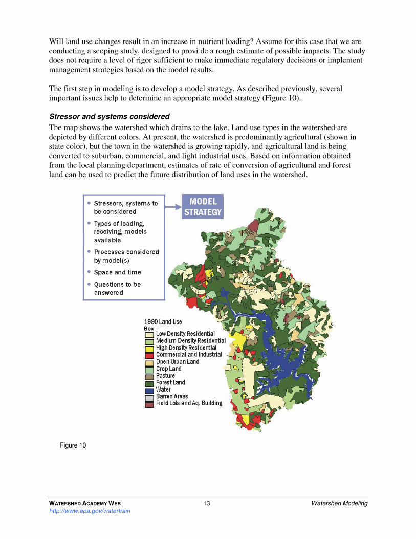
Will land use changes result in an increase in nutrient loading? Assume for this case that we are conducting a scoping study, designed to provi de a rough estimate of possible impacts. The study does not require a level of rigor sufficient to make immediate regulatory decisions or implement management strategies based on the model results.

The first step in modeling is to develop a model strategy. As described previously, several important issues help to determine an appropriate model strategy (Figure 10).

Stressor and systems considered The map shows the watershed which drains to the lake. Land use types in the watershed are depicted by different colors. At present, the watershed is predominantly agricultural (shown in state color), but the town in the watershed is growing rapidly, and agricultural land is being converted to suburban, commercial, and light industrial uses. Based on information obtained from the local planning department, estimates of rate of conversion of agricultural and forest land can be used to predict the future distribution of land uses in the watershed.

Figure 10

Box


Level of study / complexity Because the purpose of modeling is to provide an initial scoping-level estimate, rather than to make final management decisions based on model results, it is appropriate to undertake the initial modeling with a simple, but appropriate model. We know that model results will be subject to considerable uncertainty, but this is not a great concern for initial scoping. Once we see the initial results we can then decide how much additional rigor should be introduced.

A detailed, quantitative uncertainty analysis is also not needed at the scoping level. We will, however, wish to have some information on the quality of predictions in order to interpret results and make an informed decision about the need for additional modeling. For instance, if the scoping model indicates that no water quality impacts are expected will we be confident that no problems will arise, or is there a good chance that the model prediction of no adverse impact is wrong.

There are two ways to address this issue at the scoping level. On the one hand, we could structure the model with conservative (worst case) estimates of nutrient loading rates, so that we can be pretty sure that a prediction of no adverse impact means no adverse impact. On the other hand, a simple sensitivity analysis could be used to estimate the likely range of model predictions.

Spatial considerations The purpose of the scoping application is to predict nutrient loads to the lake. Therefore, it is not necessary to try to accurately predict nutrient concentrations in each tributary stream, as long as the general loading pattern is adequately represented. In addition, since this is a scoping level study, it is not critical that we separate the impact of each individual source of nutrient pollution, as it might be if the modeling was to be used to impose pollutant limitations on various stakeholders.

Time considerations The receiving water of interest is a lake, with a reasonably long residence time, and the intention of scoping is to predict an approximate average nutrient concentration in the lake in response to land use changes. Thus, we need not focus on transient changes in nutrient concentrations, but will be more interested in growing-season or yearly average concentrations. A continuous simulation model is not needed; a steady-state model should be sufficient.

Questions to be answered In sum, what is needed for the scoping analysis is a model that can predict loading of nutrients to the lake from all points in the watershed, on an annual or seasonal basis. This can be compared with existing rates of nutrient loading.

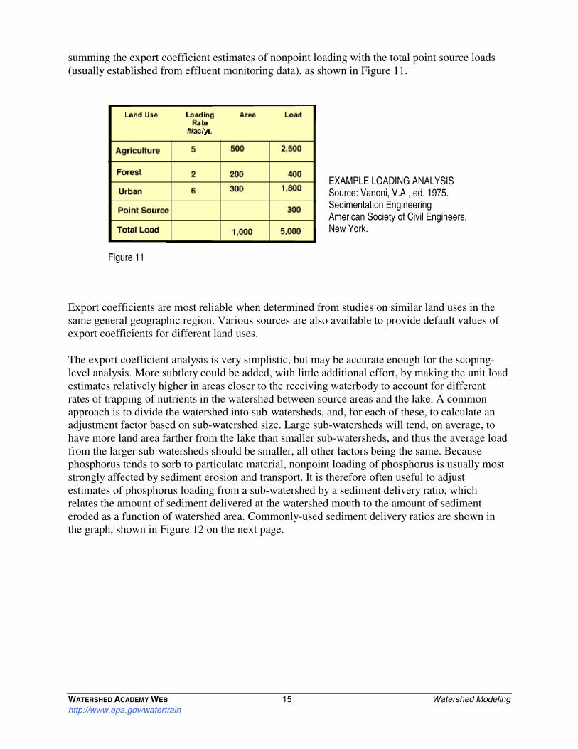
Based on the analysis of model selection considerations, an annual-average steady-state model of nutrient loading from the watershed will be sufficient. Watershed loading of nutrients can thus be described using an export coefficient model. In an export coefficient model, the average nonpoint loading from the watershed is calculated simply from a coefficient which represents an amount of load per unit area per unit time - e.g., pounds per acre per year. This unit load typically varies with land use, and its value is based on past studies, and is thus an empirical estimate. Total load to the lake under future land use conditions can then be estimated by


summing the export coefficient estimates of nonpoint loading with the total point source loads (usually established from effluent monitoring data), as shown in Figure 11.

Export coefficients are most reliable when determined from studies on similar land uses in the same general geographic region. Various sources are also available to provide default values of export coefficients for different land uses.

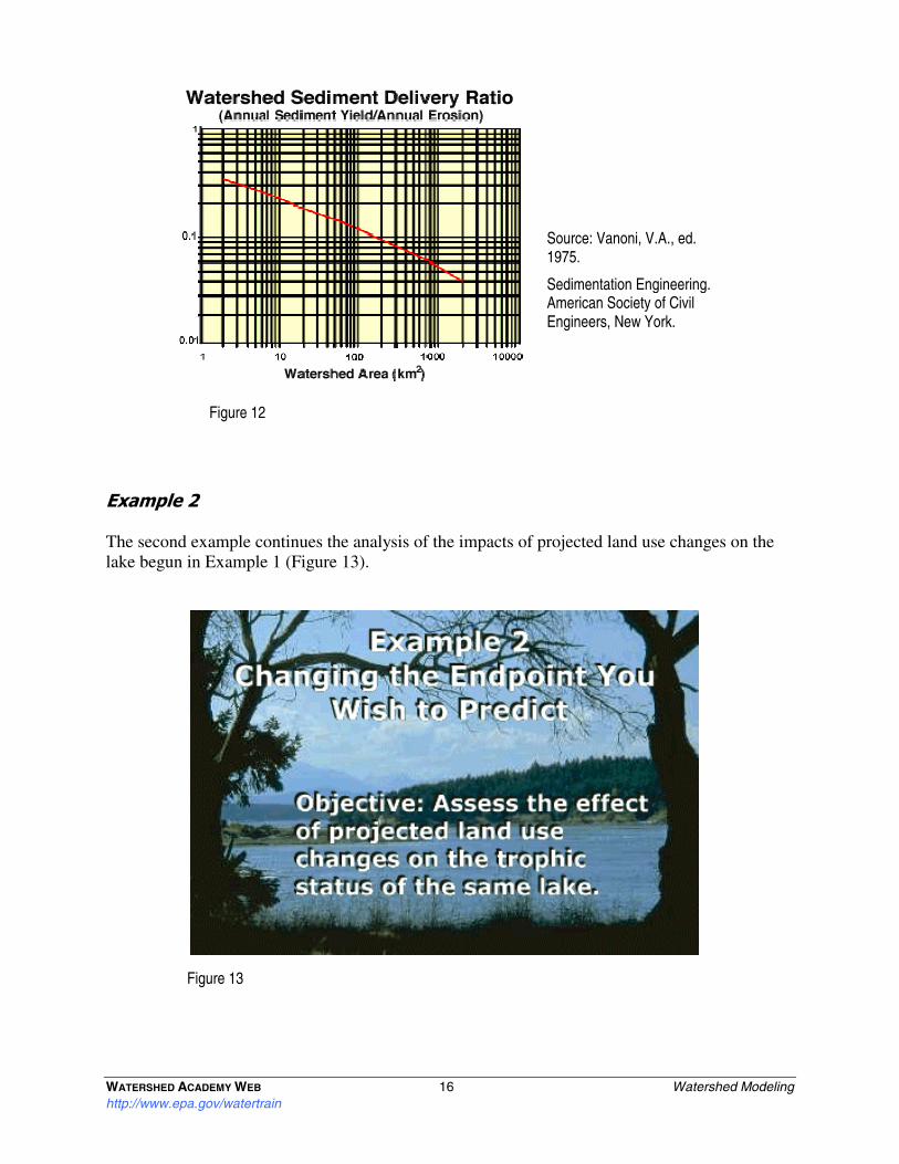
The export coefficient analysis is very simplistic, but may be accurate enough for the scoping-level analysis. More subtlety could be added, with little additional effort, by making the unit load estimates relatively higher in areas closer to the receiving waterbody to account for different rates of trapping of nutrients in the watershed between source areas and the lake. A common approach is to divide the watershed into sub-watersheds, and, for each of these, to calculate an adjustment factor based on sub-watershed size. Large sub-watersheds will tend, on average, to have more land area farther from the lake than smaller sub-watersheds, and thus the average load from the larger sub-watersheds should be smaller, all other factors being the same. Because phosphorus tends to sorb to particulate material, nonpoint loading of phosphorus is usually most strongly affected by sediment erosion and transport. It is therefore often useful to adjust estimates of phosphorus loading from a sub-watershed by a sediment delivery ratio, which relates the amount of sediment delivered at the watershed mouth to the amount of sediment eroded as a function of watershed area. Commonly-used sediment delivery ratios are shown in the graph, shown in Figure 12 on the next page.

Figure 11

EXAMPLE LOADING ANALYSIS Source: Vanoni, V.A., ed. 1975. Sedimentation Engineering American Society of Civil Engineers, New York.


Figure 13

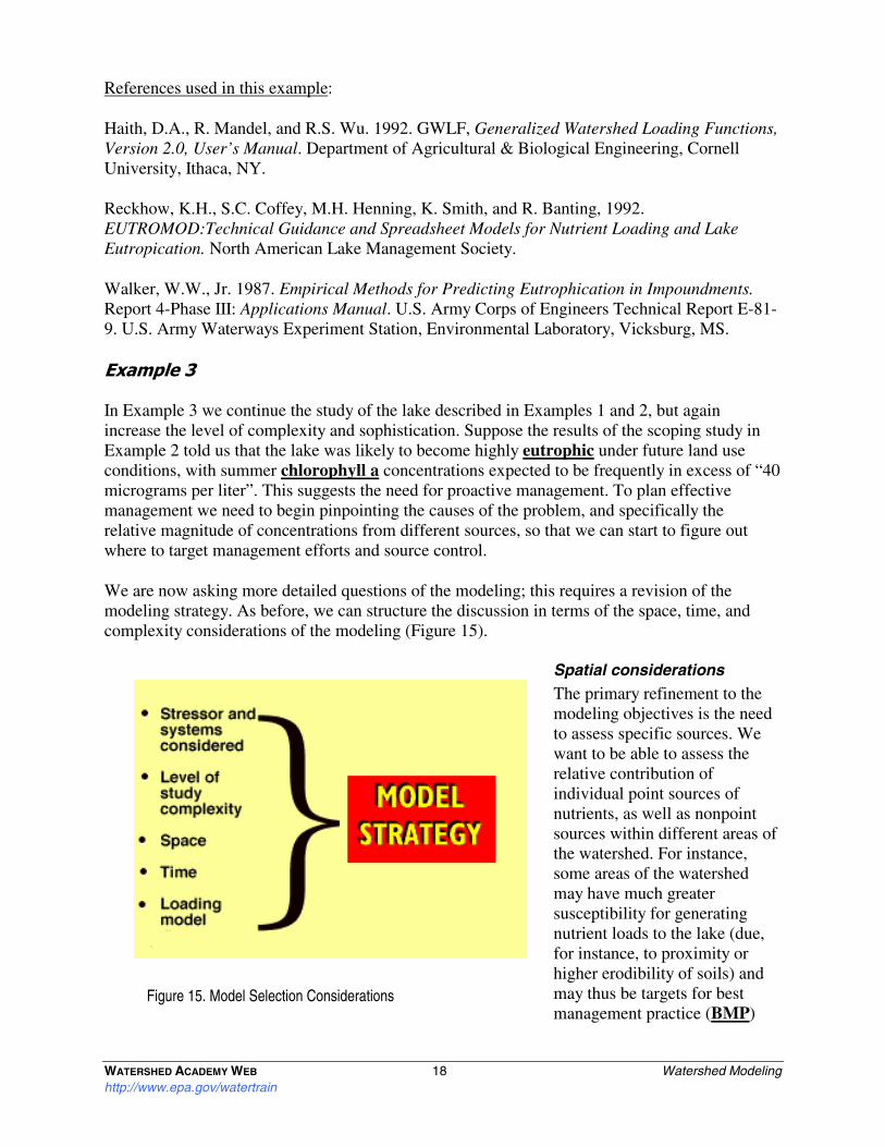
Example 2

The second example continues the analysis of the impacts of projected land use changes on the lake begun in Example 1 (Figure 13).

Source: Vanoni, V.A., ed. 1975.

Sedimentation Engineering. American Society of Civil Engineers, New York.

Figure 12


The analysis is still at the scoping level, but one additional layer of complexity is added by attempting to assess what changes in nutrient loading may imply for in-lake conditions. We have thus refined the “questions to be answered”, and need to refine the modeling strategy accordingly.

The motivation for this additional complexity is that nutrients are not in themselves the subject of our interest. Instead, nutrients are proxies for what we are really interesting in assessing: the ability of this lake to meet uses such as swimming, fishing, support of aquatic habitat, etc. The actual objectives of the assessment are often referred to as “assessment endpoints”, while the proxy measurements are referred to as “indicators”. Indicators are chosen as parameters which are closely related to assessment endpoints (i.e., nutrients are a cause of eutrophication in the lake, which can lead to impairment of uses), but are more readily measured and predicted than the assessment endpoints.

The strength of the linkage between assessment endpoints and indicators, and thus the quality of our assessment depends on which indicators are chosen. In general, indicators which are more strongly tied to the assessment endpoints provide a stronger basis for assessment. We can get closer to the actual assessment endpoints by selecting predicted trophic status as an indicator of the ability of the lake to meet its existing and designated uses.

Instead of simply predicting nutrient loads, we now want to take the loading information and use it to predict an in-lake indicator: an index of trophic status. To do this, we will need to link the loading model described previously with a receiving water model that will predict the effects of nutrient loading on the trophic status of the lake. As shown in Figure 14, predicted land use changes lead to new estimates of nutrient loads, provided by the nutrient loading model. These new nutrient loads are then used to predict trophic status using the lake water quality model.

For example, for a scoping level analysis we might use the Generalized Watershed Loading Functions (GWLF) model (Haith et al., 1992) to predict annual average nutrient loads from each subwatershed, then use these predictions as input to the Corps of Engineers BATHTUB model (Walker, 1987) to estimate (1) nutrient balance within the lake segments, and (2) average growing season algal response measured as concentration of chlorophyll a. Other, similar models such as EUTROMOD (Reckhow et al. 1992) are available which combine the loading model and receiving water response model in a single software package.

Figure 14


References used in this example:

Haith, D.A., R. Mandel, and R.S. Wu. 1992. GWLF, Generalized Watershed Loading Functions, Version 2.0, User’s Manual. Department of Agricultural & Biological Engineering, Cornell University, Ithaca, NY.

Reckhow, K.H., S.C. Coffey, M.H. Henning, K. Smith, and R. Banting, 1992. EUTROMOD:Technical Guidance and Spreadsheet Models for Nutrient Loading and Lake Eutropication. North American Lake Management Society.

Walker, W.W., Jr. 1987. Empirical Methods for Predicting Eutrophication in Impoundments. Report 4-Phase III: Applications Manual. U.S. Army Corps of Engineers Technical Report E-81-9. U.S. Army Waterways Experiment Station, Environmental Laboratory, Vicksburg, MS.

Example 3

In Example 3 we continue the study of the lake described in Examples 1 and 2, but again increase the level of complexity and sophistication. Suppose the results of the scoping study in Example 2 told us that the lake was likely to become highly eutrophic under future land use conditions, with summer chlorophyll a concentrations expected to be frequently in excess of “40 micrograms per liter”. This suggests the need for proactive management. To plan effective management we need to begin pinpointing the causes of the problem, and specifically the relative magnitude of concentrations from different sources, so that we can start to figure out where to target management efforts and source control.

We are now asking more detailed questions of the modeling; this requires a revision of the modeling strategy. As before, we can structure the discussion in terms of the space, time, and complexity considerations of the modeling (Figure 15).

Spatial considerations The primary refinement to the modeling objectives is the need to assess specific sources. We want to be able to assess the relative contribution of individual point sources of nutrients, as well as nonpoint sources within different areas of the watershed. For instance, some areas of the watershed may have much greater susceptibility for generating nutrient loads to the lake (due, for instance, to proximity or higher erodibility of soils) and may thus be targets for best management practice (BMP)

Figure 15. Model Selection Considerations


implementation or zoning restrictions on development. Accordingly, we now need a loading model with more spatial detail.

Time considerations The revised modeling objectives can still be addressed in terms of seasonal or annual average conditions, since eutrophication is a long-term process, which is relatively unaffected by short-term variability in nutrient loads. We may, however, wish to increase the sophistication of the modeling to look at average conditions in response to a variety of flow regimes. What is the range of expected responses under average, low-precipitation, and high-precipitation years?

Level of study/complexity As we move to tentative source identification in a planning-level study, certainty in model results becomes more important, because the results may be used to make decisions with economic and ecological impacts and to target future management efforts. In general, high levels of uncertainty in modeling results become less acceptable the closer we get to making real management decisions that affect stakeholders, including wastewater treatment plants which may need to install more advanced treatment, towns which may need to improve stormwater controls, and farmers who may be asked to install more BMPs.

This need to reduce uncertainty in model predictions will justify additional model complexity. Keep in mind that the rule of thumb concerning appropriate model complexity is: Do not add any more detail than is necessary. The potential need for management decisions makes more detail necessary but more data, more funds, and more expertise are required for every increment in model complexity.

One important way to reduce prediction uncertainty is to make the model more site-specific. In this example, we could continue to use the unit loads if we know for each sub-watershed the break-down of area within each land use. However, this approach is likely to maintain a significant level of uncertainty or error, since the unit loads are probably derived from averages of historical data from many areas. We can make the model more site-specific by shifting from simple export coefficients to somewhat more detailed models of runoff processes in urban and rural areas (Figure 16).

Urban runoff The dominant characteristic of urban land areas is a high percentage of impervious land cover. Precipitation runs off directly from impervious surfaces, rather than percolating into the soil, and can often transport significant pollutant loads (See www.epa.gov/OWOW/NPS/facts/point7.htm). A more sophisticated, yet still simple, approach to estimating pollutant loads generated by urban

Figure 16


areas is the use of buildup-washoff models, for which there is a well-developed literature (Novotny and Olem, Water Quality: Prevention, Identification, and Management of Diffuse Pollution). This approach is based on the observation that almost all runoff from urban areas comes from the paved or impervious area, and that most of the polluting material carried in runoff accumulates within 1 meter of curbs. Thus, between precipitation events, the model estimates the buildup or amount of material that accumulates per curb length. In addition to an increase with time, buildup may be correlated with other variables such as time of year, curb height, street width, traffic speed, atmospheric deposition rate, traffic emission rate, and frequency of street cleaning. The model then estimates the amount of washoff of material that occurs in response to a precipitation event. Washoff is correlated with rainfall intensity, and the amount of available accumulated solids.

Buildup-washoff calculations can be implemented with simple equations, but require additional data, including estimates of buildup rates and the intensity and inter-event timing of precipitation. The buildup-washoff formulation is also used within more complex simulation models, such as EPA’s SWMM (http://ccee.oregonstate.edu/swmm/).

Note that a buildup-washoff formulation is, at least in part, a representation of the actual process of pollutant load generation, rather than simply an empirical average. Such a process-based modeling technique is inherently time-variable, because it depends on the time available for buildup, and the timing and characteristics of storms which drive washoff.

Non-urban runoff Non-urban sources of runoff and pollution include agriculture (www.epa.gov/OWOW/NPS/facts/point6.htm), forestry (www.epa.gov/OWOW/NPS/facts/point8.htm), and other rural land uses. Non-urban areas are generally characterized by pervious surfaces, into which water may infiltrate. Pollutant loading is often separated into a dissolved component, which moves with the flow of water, and a sediment-attached component, which moves with the erosion of sediment. A simple process-based approach is to calculate the amount of runoff volume and the amount of erosion, then apply a concentration factor to estimate pollutant loads.

Overland runoff is often estimated with the Natural Resource Conservation Service (NRCS) Curve Number method (Ogrosky and Mockus, 1964). This method relates runoff volume to precipitation volume, antecedent soil moisture conditions, and a so-called “curve number” (CN). CN is taken from tables compiled by NRCS and depends on land use, land cover, and hydrologic soil group.

Erosion from non-urban pervious areas is often estimated using the Universal Soil Loss Equation (USLE) or one of its modifications (Wischmeier and Smith, 1978). The USLE includes factors for rainfall erosivity, soil erodibility, slope length and steepness, and land cover and management. Depending on the units used for erosivity, the USLE may be expressed on an annual or event basis. The USLE is designed to predict long-term average rates of soil losses from fields and other land uses. The rate of soil loss is not, however, the same as the yield of eroded sediment, as a substantial amount of the eroded soil may be trapped or redeposited before reaching a water body. Therefore, in watershed models the USLE is usually coupled with an estimate of fraction of sediment delivery (“delivery ratio”).


Figure 17

In many watersheds, delivery of dissolved nutrients via ground water flux is also significant, particularly for nitrogen. At the simple process-model level, simple mass balance models of precipitation infiltration and ground water delivery to streams are often used to account for ground water loading.

Use of process-based models In an attempt to reduce uncertainty in model predictions, we have moved to process-based models, albeit simple ones. These use mathematical relationships to convert data on land use, land cover, and time series of precipitation into estimates of time series of pollutant loads to a waterbody. With a process-based model of loading in hand, we can begin to examine specific management questions, such as the following:

• What effects can be expected from increasing development and impervious area? • How much can increased street sweeping reduce loading from urban areas? • What is the effect of various agricultural and erosion control practices on sediment and

nutrient loads? • What areas of the watershed generate the highest loads of pollutants?

It should be cautioned that even the most sophisticated process-based models of nutrient loading contain many empirical parameters, which cannot be measured directly. To increase confidence in model predictions, it will be necessary to go through a process of model calibration, in which model parameters are adjusted to provide a better fit to observations.

Example 4

The previous examples considered the case of nutrient enrichment of a lake, for which it was appropriate to think in terms of long-term average conditions. There are many other cases in which it is not sufficient to address only long-term averages. A typical problem in which we are concerned with short-term impacts is the case of violations of a dissolved oxygen (DO) standard in a river segment (Figure 17). The state has specified a daily average DO standard of 5 mg/l, and an instantaneous value of 4 mg/l for the protection of aquatic life. This water quality standard is being violated due to a combination of sources, and the state wishes to develop a management strategy to bring the river segment back into compliance.


As in the previous examples, model selection and model strategy are determined by a number of considerations, including stressors, and required treatment of time, space, and the level of study/complexity (Figure 18).

Stressors Depletion of DO in the river segment results from the interaction of a number of different sources of oxygen demand, including both point sources and diffuse watershed sources (Figure 18). These sources include:

1. A wastewater treatment plant, which is a permitted point source discharging a relatively steady load of oxygen-demanding waste;

2. Urban runoff routed through a separate storm sewer system, which is also a permitted point source, but discharges a highly episodic load of oxygen demanding waste;

3. Runoff from agricultural crop farming and animal operations, which constitute a diffuse nonpoint source of oxygen demanding waste; and

4. Sediment oxygen demand, exerted by organic material stored in the river sediment.

The stressors have a variety of different spatial and temporal characteristics, which will affect the choice of a model strategy.

Figure 18


Time considerations The objective of management is to prevent excursions of the DO water quality standard. This should be protected at all times, except under extraordinary conditions. Equivalently, the objective could be stated as maintaining a frequency of excursions of the standard that is below a certain acceptable low frequency, such as once in three years.

Not all the sources are constant in time, and we are concerned that the standard be met at almost all times. For these reasons, long-term average predictions of DO concentrations in the river segment do not provide us what we need to know. Instead, we need a model that will capture transient depression of DO concentrations in the river segment.

There are two ways in which we could try to capture the time-varying nature of impacts. The direct approach would be to implement a continuous model with adequate temporal resolution to predict the actual time-series of DO concentrations. This would typically require a substantial effort. The alternative is to apply a “worst-case” type of model that predicts only what happens at critical conditions, which are those conditions at which the greatest impact is expected.

In modeling the impacts of point sources a worst-case approach is typically used. This consists of assuming a minimal instream dilution capacity or design flow and applying a steady-state water quality model such as QUAL2E - which is much simpler, and less expensive to implement than a continuous model (See www.epa.gov/ORD/WebPubs/QUAL2E/). By choosing a conservative design flow and other conservative design conditions (such as the high end of the expected water temperature range, which increases oxygen demand), a wasteload allocation can be assigned to the point source, which is protective of the waterbody under most conditions. Typically, the design flow is assumed to be the 7Q10 flow which is the 7-day average low flow which recurs, on average, once every 10 years. Note that this still potentially allows occasional excursions of the DO standard, during those time periods when the instream flow is less than the 7Q10 flow.

Thus, a relatively simple method is available for the analysis of point source impacts. The addition of episodic and nonpoint sources of load (typical in watershed assessment) complicates this analysis. For these sources, lowest dilution flows and highest source loads often do not coincide, particularly when there are significant precipitation-driven sources. In these cases, the “worst case” may be at some flow higher than the 7Q10 low flow.

The simplest and most conservative approach to the watershed-scale analysis in this example would be to apply a steady-state model at the design low flow, as was done for the point source, and assume a worst-case loading from the storm sewers, agricultural areas, and other precipitation-driven sources. This would certainly be protective of water quality, but is likely to be unrealistic, since maximum loading from the runoff would normally be associated with higher than 7Q10 flows in the river. Indeed, such an ultra-conservative approach is likely to suggest that there is no assimilative capacity available for the point source, even when observations indicate that this is clearly not the case.

To make the modeling assessment more realistic, while continuing to use a simple, conservative approach we could run two steady-state model applications, intended to represent the range of expected impacts in the receiving water segment. The first application would be intended to reflect the impact of the point source at drought condition flows, with no contribution from episodic precipitation-driven sources. The second model application would be designed to reflect


the impact of nonpoint loading during a large runoff event, plus the point source. To make this application conservative (but not completely unrealistic) we would combine the large runoff loads with an unusually low dilution flow for such an event in the receiving water. One way to do this is to analyze historical records of flows during large rain events, and choose the lowest instream flow (or once-in-10-years recurrence flow) observed in association with large rain events.

Alternatively, the results can be made more realistic by running a continuous simulation model that will provide a full representation of the correlation of runoff events and instream flows. Continuous modeling allows us to assess the interaction of point sources and nonpoint sources over all flow conditions, including the period following a runoff loading event when flow drops off, but concentrations may be high. The main drawback of using a continuous modeling analysis is the additional data, time, and user expertise required to implement it.

The choice of which method to use will depend on the level of detail required to answer the question at hand, and the resources available for the assessment.

Model linkage considerations Developing a watershed modeling tool for this example will require linking several different types of models together. Or, we may be able to use an existing software package that has all these parts already linked together (i.e., it includes sub-models for each of the components) (see Figure 19 on the next page). The three main types of models which must be linked are:

1. A model for flow and pollutant loading in urban runoff;. 2. A model for flow and pollutant loading in rural runoff; and 3. A model of the receiving water body, which calculates the effects of oxygen demanding,

loads on DO in the river segment.

Spatial detail As with the previous example of the lake, the amount of spatial detail we need to include depends largely on how well we wish to be able to separate out the effects of different sources. This is less important at the scoping level, when one perhaps only wishes to assess the approximate severity of a problem, but more important when results of the modeling study will be used to evaluate management strategies. For instance, we may wish to consider the potential effectiveness and trade-offs between reducing overall input of BOD via requiring a higher level of treatment at the wastewater treatment plant, implementing street cleaning to reduce urban stormwater loading, requiring the town to build infiltration basins to reduce the total flow and loading from urban areas, or encouraging more use of best management practices in agricultural areas. A model is a useful tool for comparing the effectiveness of various possible control options. However, to make the comparison the model must include sufficient complexity to assess the relative impacts, and interactions of individual sources.


Example 5

We will now move on to a more complex example in which the joint impacts of many sources must be considered. This example addresses a large (7,000 square mile) watershed which contains many point sources, including wastewater treatment plants and industrial discharges. There are also urban and rural sources of nonpoint load, including combined sewer overflows (CSOs), separate storm sewer systems, septic systems, and runoff and groundwater flux from agricultural fields and animal feed lots. In the estuary at the downstream end of this watershed massive fish kills are occurring as a result of a complex interaction of natural tidal events with eutrophication caused by nutrient inputs. The nutrient loads promote excessive algal growth, including some toxic species. In addition, algal die off, particularly at the salt-freshwater interface, exerts a large oxygen demand and results in intermittent depressed dissolved oxygen levels. Degraded conditions in the estuary are attributed primarily to excess nitrogen loads, which derive from the entire watershed.

Figure 19 Model Components


The state wishes to reduce nutrient inputs to the estuary, but must decide by how much, and how to do it (Figure 20). A key question is who bears the burden of additional pollution controls? There are many stakeholders in this watershed who would be affected by any management decisions. The issue is contentious: agricultural interests in the lower watershed claim that problems are due primarily to increased wastewater flows from rapid growth in upstream urban areas, and they should not have to bear the costs of management. The urban areas blame agriculture and contend that loads from their plants are significantly attenuated before reaching the estuary, and it would be unfair to restrict their ability to grow. Landowners in rural areas are afraid that nutrient restrictions will preclude them from developing their property. Meanwhile, fishermen and the tourist industry in the estuarine area are losing money and demanding immediate action.

In such a contentious atmosphere, with major financial interests at stake, any modeling prediction which appears to favor one stakeholder group’s point of view is likely to be challenged by other groups in the watershed, who may claim that the results of the model are too uncertain to justify the restrictive measures the state wishes to impose on them. Because of these

Figure 20. Controlling Eutrophication in a Large Watershed

Photo: USDA Develop a strategy to significantly reduce nutrient inputs to a river in a large watershed with many sources and diverse stakeholders.

Objective


demands, and the need for defensibility in results, it is judged that a high level of complexity is warranted in the modeling application.

This case demonstrates that the stakeholders or affected parties will often drive the nature and complexity of a watershed modeling study. Even though it may be possible to reach a correct management decision using a simpler scoping model this will not provide a high enough degree of certainty to justify politically difficult management decisions. A high degree of model complexity may be required to assure all stakeholders that their interests are being addressed.

Model selection considerations for this case may be summarized as follows:

Stressors The stressor of interest is nitrogen loading. Nitrogen is linked to support for uses through eutrophication in the estuary. A means of predicting algal response to nitrogen loads is also required; however, it may be advisable to handle this component separately by first determining an acceptable target nitrogen load at the estuary head, then using the watershed model to assess attainment of the target load.

Time considerations There is a fairly long lag time in estuarine response, and estimates of loading to the estuary at the time scale of weeks would be sufficient. However, some important watershed sources are precipitation driven, and contention over the importance of these sources may demand use of a continuous (daily time step) simulation model driven by precipitation data. The model will, however, need to be run over a long time series of precipitation data (decades) to derive a reasonable estimate of the efficacy of control strategies under the expected range of meteorologic and hydrologic conditions.

Spatial considerations Both types of land use and the location of these land uses within the watershed are at issue in evaluating management options. Therefore, good spatial resolution of land uses is required, using a GIS-based approach. Evaluating loss or attenuation of nitrogen loads during transport in stream will require use of an appropriate river model. Finally, ground water can be an important pathway for transport of nitrogen, so the model must also be able to address surface-ground water interactions.

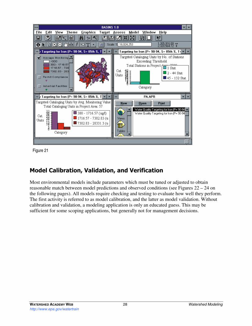
The model strategy for this case requires linking of a GIS-based continuous model of watershed nitrogen loading with a continuous model of river transport. This is accomplished using the EPA model BASINS (See: www.epa.gov/OST/BASINS). BASINS combines spatially distributed land use data, EPA’s Reach File 1, and the HSPF simulation model for watersheds and rivers into a convenient package with an ArcView GIS interface (see Figure 21 on the next page). Only by using the power of a GIS interface is it convenient to undertake a continuous simulation model of such a large watershed. (Note that the ability to address routing of stream flows and transformations of pollutant loads during stream transport is included in BASINS Version 2, currently undergoing testing and scheduled for full release in early 1998).


Model Calibration, Validation, and Verification

Most environmental models include parameters which must be tuned or adjusted to obtain reasonable match between model predictions and observed conditions (see Figures 22 – 24 on the following pages). All models require checking and testing to evaluate how well they perform. The first activity is referred to as model calibration, and the latter as model validation. Without calibration and validation, a modeling application is only an educated guess. This may be sufficient for some scoping applications, but generally not for management decisions.

Figure 21


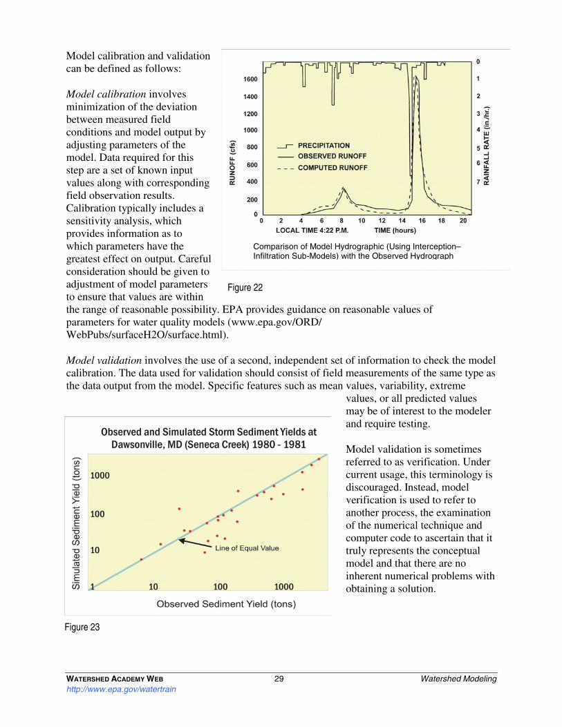
Model calibration and validation can be defined as follows:

Model calibration involves minimization of the deviation between measured field conditions and model output by adjusting parameters of the model. Data required for this step are a set of known input values along with corresponding field observation results. Calibration typically includes a sensitivity analysis, which provides information as to which parameters have the greatest effect on output. Careful consideration should be given to adjustment of model parameters to ensure that values are within the range of reasonable possibility. EPA provides guidance on reasonable values of parameters for water quality models (www.epa.gov/ORD/ WebPubs/surfaceH2O/surface.html).

Model validation involves the use of a second, independent set of information to check the model calibration. The data used for validation should consist of field measurements of the same type as the data output from the model. Specific features such as mean values, variability, extreme

values, or all predicted values may be of interest to the modeler and require testing.

Model validation is sometimes referred to as verification. Under current usage, this terminology is discouraged. Instead, model verification is used to refer to another process, the examination of the numerical technique and computer code to ascertain that it truly represents the conceptual model and that there are no inherent numerical problems with obtaining a solution.

Figure 23

Figure 22

Comparison of Model Hydrographic (Using Interception–Infiltration Sub-Models) with the Observed Hydrograph


A variety of statistical tests are available for assessing model goodness of fit during calibration and validation. A useful introductory summary is provided in: Reckhow, K.H., J.T. Clements, and R.C. Dodd. 1990. Statistical evaluation of mechanistic water quality models. J. Environ. Eng., 116(2): 250-268.

How Do We Deal With the Added Complexity?

Watershed assessment may require additional complexity beyond traditional modeling exercises for the evaluation of point source impacts. Looking back over our examples, we can see that modeling at the watershed level can add complexity for several reasons:

• Involvement of diverse stakeholders who demand a certain level of modeling detail and certainty

• The need to consider nonpoint source loading of pollutants from land areas

• The need to consider multiple sources of stressors

• Sometimes (though not necessarily), watershed modeling requires representation of greater spatial and temporal detail than a point source problem. Often there will be interaction between point sources and episodic nonpoint sources which may require evaluation of temporal patterns. In addition, evaluating management options may require separating out the effects of many different sources.

How can limited resources be stretched to handle the additional demands of watershed modeling? While watershed management can add levels of complexity to the jobs of assessment and modeling, it also provides a number of new opportunities for partnerships with other agencies and groups, allowing the state to deal with water quality problems more effectively (see Figure 25 on the next page). You can be more cost-effective by drawing on existing expertise in other agencies and organizations (e.g., using agricultural agency expertise on runoff processes). You can also be more effective by leveraging resources through monitoring consortia or watershed associations. A watershed model may be more complex than a point source model, but may be useful for the evaluation of multiple sources within a watershed. These arrangements allow you to reduce duplication, be more strategic with monitoring plans, and leverage available lab resources. In many cases, you may also be able to pool public and private funds to conduct

Figure 24


joint analyses. This type of jointly funded study has the added benefit that when you get buy-in at the beginning, the stakeholders are more likely to accept the results.

Overarching Principles

This module concludes by reviewing some of the important points discussed above in the form of some overarching principles to follow when choosing appropriate models for watershed assessment.

1. Have a clear statement of project objectives and verify the need for modeling. (Figure 26)

Ask yourself: How can a model help address the questions and problems relevant to decisions? How can a model be used to link stressors or management actions to quantitative measures (endpoints) of waterbody condition? Is modeling appropriate for examination of the stressors of concern in this situation?

Some of the types of problems for which modeling could be useful include:

• Quantifying loads from nonpoint sources • Estimating load reductions needed to

meet a water quality standard • Establishing a total maximum daily load

(TMDL) • Distinguishing between levels of

effectiveness of different management strategies

• Determining if management criteria can be met by a proposed strategy.

Remember that, where practically and economically feasible, real data are always preferable to model predictions as a basis for decisions.

Figure 25

Figure 26


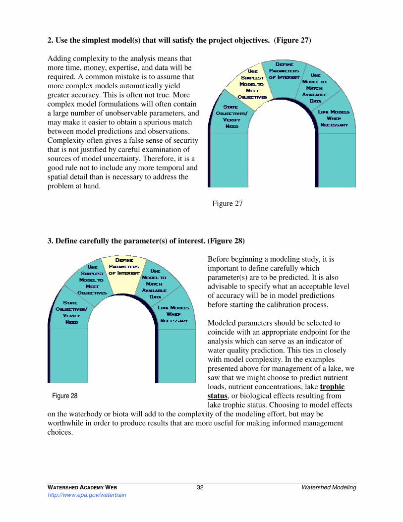
2. Use the simplest model(s) that will satisfy the project objectives. (Figure 27)

Adding complexity to the analysis means that more time, money, expertise, and data will be required. A common mistake is to assume that more complex models automatically yield greater accuracy. This is often not true. More complex model formulations will often contain a large number of unobservable parameters, and may make it easier to obtain a spurious match between model predictions and observations. Complexity often gives a false sense of security that is not justified by careful examination of sources of model uncertainty. Therefore, it is a good rule not to include any more temporal and spatial detail than is necessary to address the problem at hand.

3. Define carefully the parameter(s) of interest. (Figure 28)

Before beginning a modeling study, it is important to define carefully which parameter(s) are to be predicted. It is also advisable to specify what an acceptable level of accuracy will be in model predictions before starting the calibration process.

Modeled parameters should be selected to coincide with an appropriate endpoint for the analysis which can serve as an indicator of water quality prediction. This ties in closely with model complexity. In the examples presented above for management of a lake, we saw that we might choose to predict nutrient loads, nutrient concentrations, lake trophic status, or biological effects resulting from lake trophic status. Choosing to model effects

on the waterbody or biota will add to the complexity of the modeling effort, but may be worthwhile in order to produce results that are more useful for making informed management choices.

Figure 27

Figure 28


It is also important to be sure that predictions will be available in appropriate units (e.g., dissolved versus particle-attached concentrations, daily versus annual average concentrations) for use in decision making. For example, for a eutrophication analysis it may be sufficient to predict total phosphorus concentrations on a seasonal average basis, while a wasteload allocation to prevent metal toxicity may require predicting the dissolved-phase concentration of the metal on a continuous basis.

4. To the extent possible, use a prediction method consistent with available data. (Figure 29)

Data availability should be evaluated before beginning the model selection process. Models selected for analysis should have input requirements which match up well with data which is already available, or which can be collected in the course of the study.

5. It will often be necessary to use multiple models or link models to address watershed assessment problems. (Figure 30)

As we have seen in the examples, it is often necessary to use one model to predict loading to a waterbody from nonpoint sources, and a second model to predict fate and transport of pollutants in the waterbody, and possibly a third model to predict effects of the pollutant on biota or communities. It is important to choose models with compatible data input/output. For instance, if the fate and transport model requires daily load values, then the loading model should provide daily output of the appropriate parameters.

Figure 29

Figure 30


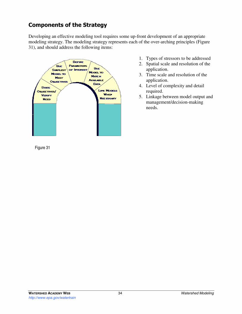
Components of the Strategy

Developing an effective modeling tool requires some up-front development of an appropriate modeling strategy. The modeling strategy represents each of the over-arching principles (Figure 31), and should address the following items:

1. Types of stressors to be addressed 2. Spatial scale and resolution of the

application. 3. Time scale and resolution of the

application. 4. Level of complexity and detail

required. 5. Linkage between model output and

management/decision-making needs.

Figure 31


Glossary of Underlined Terms

Pervious & Impervious Surfaces: Pervious surfaces allow water to penetrate or infiltrate into the underlying soil or rock. Impervious surfaces do not allow water to pass through. For instance, tiled soil is highly pervious, while asphalt is impervious.

Eutrophication: The process of physical, chemical, and biological changes associated with nutrient and organic matter enrichment of a water body. Most frequently used to refer to nuisance growth of algae or other aquatic plants associated with nutrient enrichment.

Chlorophyll a: A green pigment used by algae and green plants during the process of photosynthesis to convert light, carbon dioxide, and water to sugar. Chlorophyll a concentration is often used as an approximate index of algal biomass.

Trophic Status: A measure of the degree of eutrophication of a water body.

BMPs: Best Management Practices

7Q10 Flow: The 7-day average low flow which recurs, on average, once every 10 years.

POTW: Publically Owned Treatment Works

Erosivity: The susceptibility of a surface to be eroded or worn away.

Documents

WATERSHED ACADEMY WEB - cfpub.epa.gov · PDF fileWatershed Academy Web, found at . To the extent ... Is modeling needed to scope or quantify a problem?