WATER RESOURCES DIVISION I ESTIMATING STEADY-STATE ... · The dependence of relative evaporation rates, 17 E/E po t' upon the potential evaporation rates, E po t' for 18 Chino clay-----29

I v~ I

eFT<~ f'f*f{J

I I I I I I I I I~ I~ .-

IcC I I I I I I

UNITED STATES DEPARTMENT OF THE INTERIOR

GEOLOGICAL SURVEY WATER RESOURCES DIVISION

ESTIMATING STEADY-STATE EVAPORATION RATES FROM

BARE SOILS UNDER CONDITIONS OF HIGH WATER TABLE

BY

C. D. RIPPLE, J. RUBIN AND T. E. A. VAN HYLCKAMA

OPEN-FILE REPORT

Wa.tvr. RcuoUJtee6 fJ.iv.U.ion Mualo J'aJtk, Cali6o!UUa.

1910

- -

l.128) I I I I I I I I I I I I I I I I I I

2

3

4

5-

6

7

8

9

10-

11

12

13

14

15-

16

17

18

19

Contents

Page

Symbols----------~---------------------------------------------- iii

Abstract-------------------------------------------------------- 1

Introduction------~--------------------------------------------~ 2

Theory-------------------------.--------------------------------- 4

Meteorological equation----------·-------------------------- 5 Soil equation---------------------------------------------- 8

Application-----------------------------------------------------· 14

Data required--------------------------------------------~- 14 Homogeneous soil---------------------------------------•--- 17 Layered soil----------------------------------------------- 30 Effects of vapor·transfer---------------------------------- 36

Discussion, experimental test; and conclusions-------------.----- 46

Appendix: Flow charts for es.timating steady-state evaporation rates from bare soils-------------------- 58

References------------------~----------------------------------- 60

Illustrations

Figure 1. The water-table-soil-atmosphere systems considered:

Case A. A homogeneous soil with water transferred

20- exclusively in liquid form; Case B. A layered soil with

21

22

23

24

25--

water transferred exclusively in liquid form; Case c.

A homogeneous soil with water transferred in liquid and

vapor forms------------------------------------------------9

ll. S. GOVERNMENT PIUNTING OFFICE: 1959 0-511171

867-100

i

I I I I I I I I I I I I I I I I I I

Page

1 n

2 Figure 2. Dimensionless plots of f·= f(e) = (e+l) (;1) ---- 19 3

yu 4 Figure 3. Dimensionless plots. of I = I(y ) = r ...2L. u

Jo 20

yn+l 5-

6 Figure 4. Dependence of dimensionless soil water suction, s,

7 on dimensionless soil height, z: A. Soil parameter n = 2;

8 B. Soil parameter n = 5----------------------------------- 21 9 Figure 5. Plots relating dimensionless evaporation, e, to

10- dimensionless depth to water ·table, .(,---------------------- . 23-

u Figure 6. The intercept method for determining evaporation

12 rates: A. Chino clay; B. Buckeye soil------------•----- 25

13 Figure 7. Dependence of evaporation rates on water table

14 depths, calculated by intersection method (solid lines).:

15- A. Chino clay; B. Buckeye soil--~--------------------•-- 27

16 Figure 8. The dependence of relative evaporation rates,

17 E/E t' upon the potential evaporation rates, E t' for po po

18 Chino clay------------------------------------------------- 29

19 Figure 9e The influence of layering on the relation between

20- evaporation rate and depth to water table: i. the

21

22

23

24

25·-

homogeneous case(~= 0); ii. a two-layered soil;

iii. a three-layered soil.,.·-------------------------------- 37

Figure 10. Comparison of actual versus estimated evaporation·

rates for a given depth to water table--------------------- 53

ii

II. S. GOVERNMENT PHINTING OFFICE: 1959 0- 511171

867 ·100

I~ ·:>r:.·l

I I I I I I I I I I.

I I I I I I I I

;a

I

Symbols

= a subscript, indicating a variable determined in the air,

H em above the soil surface. a

I = a subscript, indicating a variable determined at the soil :u I

surface.

.v = a subscript, indicating a variable which involves water

I

b

B

c

D a

=

=

=

=

=

vapor transfer.

..a -1 sensible heat transfer into the air, cal em day -·

-B(Tu - ~) /L~, gm em -4

-3 0 -1 (1'\/cr) (C/o.)s', gm em K •

E/Dhv' em -1

I a coefficient characterizing the molecular diffusion of watert

! a -1

vapor in free air, em day

Dhv = a coefficient characterizing the molecular diffusion of a -1

soil-water vapor caused by humidity gradients, em day •

DTv = a coefficient characterizing the molecular diffusion of

e

E

e pot

E pot

E co

f(e)

=

=

=

=

=

a -1 o -1 · soil-water vapor caused by thermal gradients, em day K •·

E/K t' rate of evaporation from the soil, dimensionless. sa -1

rate of evaporation from the soil, em day •

rate of potential evaporation, dimensionless.

-1 rate of potential evaporation, em day soil-limited ~'-&tias~rate of evaporation from the soil, dimensionless.

soil-limited ,_ f · f h 1 day~1 = ·2i j tirg.Arate o evaporat~on rom t e soi , em

= a functional relation defined by equation 27.

• t.l..l\( ti'"·l ':· •j, , :• ! II'

iii

1 .. : ;•1';7

I I I I I I I I I I.

I I I I I I I I

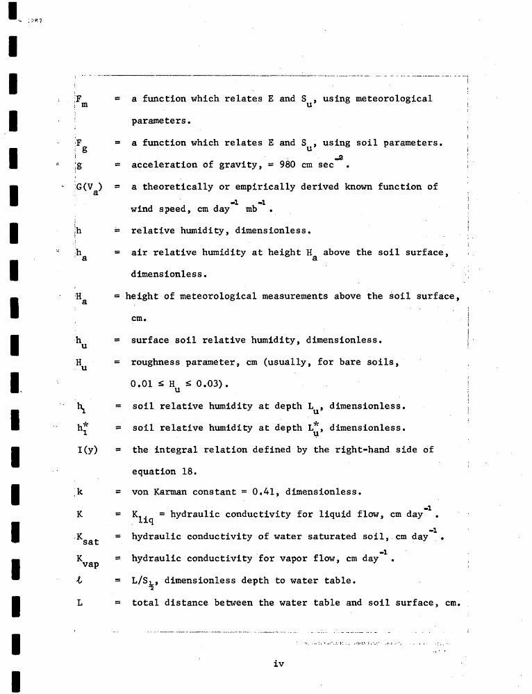
I ... -------·-----~------·-·-·-------------·· ..... - .... ·-·- .... -.--.............. , = a function which relates E and S , using meteorological

u

parameters.

= a function which relates E and su' using soil parameters.

..a = acceleration of gravity, = 980 em sec

·· ;G(V a) = a theoretically or empirically derived known function of

-1 -1 wind speed, em day mb

= relative humidity, dimensionless.

= air relative humidity at height H above the soil surface, a

dimensionless.

1H = height of meteorological measurements above the soil surface, a

em.

·h = surface soil relative humidity, dimensionless. u

.H = roughness parameter, em (usually, for bare soils,

.u

h* 1

=

=

0.01 S H s 0.-03). u

soil relative humidity

soil relative humidity

at depth L , dimensionless. u

at d.epth L *, dimensionless. ~

I(y) = the integral relation defined by the right-hand side of

K

.K sat

K vap

L

=

=

=

=

=

=

equation 18.

von Karman constant = 0.41, dimensionless.

Kliq = hydraulic conductivity for liquid flow, em day -1

hydraulic conductivity of water saturated soil,. em day -1

hydraulic conductivity ·for vapor flow, em day -1

L/S%' dimensionless depth to water table.

total distance between the water table and soil surface, em.

.. ; • ' '. : \ 1·. I'~ •. \. 1·: • • ' • H i.'.. ! 11 .. •• • • ~· l : •. I

.. [.'

iv

I . ;·~. 1


r·--·-··-- .. -------·------...,...----- ---------------·---------------- ------.--. ! I

I

i L. = in the multilayer case, the thickness of soil layer, em, j

layers above ~he water table (that is, j = 1 means one layer i

J

1 above the water table, etc.). I jL = thickness of the uppermost soil layer, em. : u I

iL* = thickness of the uppermost portion of the dry soil surface I U

at which ~ was determined, em.

:L' = thickness of the dry soil layer in which isothermal vapor u

transfer is assumed to predominate, em.

-1 :M = molecular weight of water = 18 gm mol • ;

n = an integer soil coefficient which usually ranges from 2 for

clays to 5 in sands.

p = saturation vapor pressure of water, mb.

. p(T) = a known relation between the saturation water. vapor .

pressure and temperature (given in tabular or functional

form), mb.

P = ambient pressure, mb (taken asP= 1000mb in this study).

q = flux of water, em day -1

-2 -1 Qg = soil heat flux into the ground, cal em day

R

s

s

~ = net radiative flux received by the soil surface, cal em

=

=

=

-1 day •

7 0 -1 gas constant = 8.32 x 10 erg K •

S/S~, dimensionless suction. 2

soil water suction, defined as the negative of the soil water

pressure head, em of water.

Sj = in the multilayer case, the soil water suction at the upper

interface of layer j, em of water.

1,1 • .'! ,,·.'·'

v

I


s u

T

T a

T u

:r,.

y

z

=

=

=

=

=

=

=

=

=

=

water suction at the soil surface, em of water.

a constant soil coefficient representing S at K = L K ":! sat'

em of water.

temperature, °K. . 0

air temperature at H , K. . a

surface soil temperature, °K.

soil temperature at depth L:, °K. wind speed at height H , em day

a -1

a variable, defined by equation 16.

a variable, defined in conjunction.with the right-ha~d side

of equation 31 of the layered ·Soil case.

Z/S~,· dimensionless height above water table.

Z = vertical height above the water table, em.

=

s I =

y =

e: =

tortuosity factor, dimensionless.

...:3 0 -1 d(log p )/dT, gm em K e v

psychrometric constant, 0 -1

0.000659 P, mb K

water/air molecular ratio= 0.622 (dimensionless).

C = a ratio of the average temperature gradient in the air-filled

11

A.

p v

soil pores to the overall soil temperature_ gradient,

dimensionless.

= soil porosity, dimensionless.

-1 = latent heat of vaporization of water at T , cal gm

a -3 = air density at T , gm em

a ...:3

= P (T) = density of saturated water vapor, gm ern p is a v . v

function of temperature. -·· . - ...

vi

·-··· .. -- -¥·--- .. :... ·--... ·----· ---------~-- -·-··-...:.--~...,..----··.

= . . . -'3

water density at appropriate T, grn em

= volumetric air cqntent of the soil, dimensionless.

= a dimensionless function defining the effectiveness of the

water-fl;'ee ·pore· space for diffusion.

1,. ' , 1 .' ~ I , ', · : '•i. : I J• ' , . • ··~ 1 ~ •l ; ,

vii

., I

l

,,126)


2

3

4

b

7

H

1.:1

11

l4

lb

l i

I~

i9

:.'.1

5 ..

I I

I ESTIMATING STEADY-STATE EVAPORATION RATES FROM I I

I BARE SOILS UNDER CONDITIONS OF HIGH WATER TABLE

I

I

By C. D. Ripple, J. Rubin and T. E. A. van Hylckama

I i

10- I t

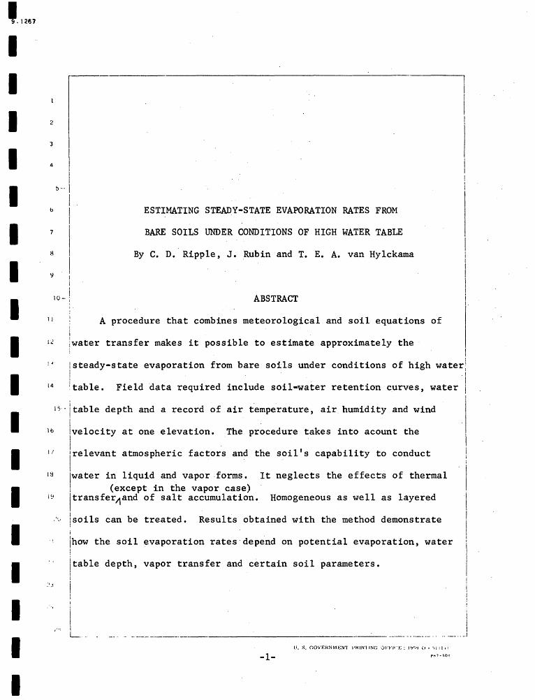
ABSTRACT I

I I

i A procedure that combines meteorological and soil equations of

!water transfer makes it possible to estimate approximately the

I I

I I i I

I I I.

! I steady-state evaporation from bare soi·ls under conditions of high water; I, . · . i .I 1table. Field data required include soil-water retention curves, water 1

1?· • j table depth and a record of air temperature, air humidity and wind

~velocity at one elevation. The procedure takes into acount the

~relevant atmospheric factors and the soil's capability to conduct

'water in liquid and vapor .forms. It neglects the effects of thermal , (except in the vapor case) · ltransfer~and of salt accumulation. Homogeneous as well as layered

.''-· I soils can be treated. Results obtained with the method demonstrate I I

!how the soil evaporation rates·depend on potential evaporation, water I l

Jtable depth, vapor transfer and certain soil parameters. i

I i I

·. I L .. -------------- --- ··-··-· ·····---- .... ___ ,,

!1. S. GOVEHNMI::NT I'HIN'IING OFVI"J-:: I'I~Y 0 ·~Ill,:

-1-

I


r :

. ····--·- ····--·------· -------... --· . . . .. ................. ··----·

INTRODUCTION

It is sometimes desirable to estimate the evaporation rates from

bare land surfaces and to predict approximately the variation of these

rates with meteorological conditions or with man-imposed changes in the

water table level.· This might be rather important in certain regions

during the appraisal of ground water availability. For such purposes,

it is often both permissible and useful to use relatively simple

estimation methods. One~ possibility is to assume steady state of·

the hydraulic-gradient driven, upward flux of water and to neglect

certain effects of soil temperature and of solute accumulations.

The basic approaches required for the development of this method

can be found in the literature. Gardner (1958) suggested a convenient

equation for describing hydraulic conductivity, the most relevant soil

parameter, and from it developed methods for evaluating soil-limited

evaporation in cases of high water table. Anat and others (1965) and

Stallman (1967), employed Gardner's general approach, but different

soil parametric equations. They demonstrated the usefulness of

dimensionless curves in solving problems of the type under consideration.

The above treatments stressed the cases in which soil properties

were the determining factor as far as evaporation is concerned. Cases

of evaporation in which the atmospheric conditions play the decisive

role can be treated by means of several, purely meteorological equation,s

(for example, Sla~yer and Mcilroy, 1961).

\ ,·, I..•(''J'I 'I,; i

-2-

1 .. 1 : ;·~ 1

I ·------,..---------------·-----------------. ----·-· .... -------------

I Philip {1957a, b) showed how the effects of the soil factors on

I bare-soil evaporation coupled with those of the atmospheric parameters.,

I i l Due to utilization of numerical methods, his approach to soil influenceis

I iwas more general but mathematically less convenient than the one of I

I .• i Gardner.

All of the studies quoted above concerned themselves with

I homogeneous soils and mainly with cases involving liquid transfer.

Gardner indicated how to include the vapor-transfer effects, but only

I for selected circumstances. Philip's approach to vapor effects is more·

I general, but again mathematically less convenient.

It is the purpose of this paperto integrate and extend the above

I approaches for estimating steady-state evaporation from bare soils

under high water table conditions. The past approaches are unified,

I modified and supplemented when necessary to improve their practicability

as a general {though approximate) me·thod.

I Stress has been placed on use of readily available data, simple

I parameter-determination techniques, dimensionless variables and simple

graphical or algebraic treatments. Numerical integrations have been

"I avoided. The older approaches are generalized so as to make them

applicable to layered as well as homogeneous soils. In addition,

I analysis of the multilayer case is modified to allow for the treatment

I of evaporation affected by water vapor transfer. Examples of the

results obtained with the suggested method are presented, discussed and

I utilized for demonstrating the· role of some of the relevant factora.

I -3-I ; ~ ) \• J• t \ \ ' • ' ; •I i ~ • 'I ,• t

I

I .·r •'

I I I I I I I I I I I I I I I I I

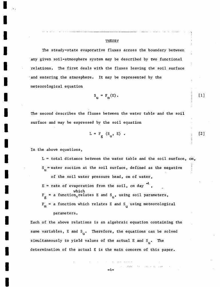
THEORY

The steady-state evaporative fluxes across the boundary between

·any given soil-atmosphere system may be described by two functional

relations. The first deals with the fluxes leaving the soil surface

'and entering the atmosphere. It may be represented by the

meteorological equation

S = F (E). u m

The second describes the fluxes between the water table and the soil

surface and may be expressed by the soil equation

In the above equations,

L = F (S , E) • g u

L = total distance between the water table and the soil surface, em,

S =water suction at the soil surface, defined as the negative u

of the soil water pressure head, em of water,

-1 E = rate of evaporation from the soil, em day

which Fg = a functionArelates E and Su' using soil parameters,

F = a function which relates E and S using meteorological m u

parameters.

Each of the above relations is an algebraic equation containing the

same variables, E and S • Therefore, the equations can be solved u

simultaneously to yield values of the actual E and S • The u

determination of the actual E is the main concern of this paper.

~ ' i, I\· •

-4-

i·

!

[ 1]

[2]

I. I I I I I I I I I I I I I I I I I I

·'"' 1

Meteorological Equation

A relation is sought to express meteorological equation 1.

:However, for simplicity and ease of handling, it is best to treat

1 the components of this relation individually.

The basic meteorological equation used is of the type generally

known as the bulk aerodynamic, or Dalton equation (Slatyer and Mcilroy,!

: 1961). I I

Its form is I

where

G(V ) = a theoretically or empirically derived, known function a

v a

-1 -1 of wind speed, ern day rnb

= wind speed at height H , ern day a

-1

h = relative humidity, dimensionless,

T

p

p(T)

a

u

0 = temperature, K,

= saturation vapor pressure of water, mb,

= a known relation between the saturation water vapor

pressure and temperature (given in tabular or functional

form) , rnb,

= a subscript indicating a variable determined in the air

H ern above the soil surface, a

= a subscript indicating a variable determined at the soil

surface.

I ~ ' . • , ··!·!1•

-5-

[3]

I '. r. ~ .•

I I I I I I I I I I I

:·.

I I I I I I

-----·-·---·--·-------·----------·-···--- -·- -- ......... _______ ~ ....... "'1

This equation, due to its simplicity, has been used extensively for

estimating the loss 9f water by free-water surfaces, plants, and bare

Either soils. ~{its empirical fontl (Harbeck, 1962) ·'Or one of its modified

can be :forms (Slatyer and Mcilroy',· 1961, p. 3-40 to 3-44) 11 ka 1 ein~· employed.

The present study utilized.the·wind function used by van Bavel

(1966)'

:a

G(Va) = (:wa :k) __ v_a....._ __ · (log H /H )2

e a u

·where

p air density at T , ~

= gm em a a -3

Pw = water density at T gm em a

€ = water/air molecular ratio = 0.622, dimensionless,

k = von Karman constant = 0.41, dimensionless,

p = ambient pressure, mb (taken as P = 1000 mb in this study),

' I

[ 4]

H = height· of meteorological measurements, above the soil surface·, em, · a

H = roughness parameter, em (usually, for bare soils, u

0.01 ~ H ~ 0.03)~ u

Equation 3 may be rewritten as follows in order to obtain the

form required by equation 1

h __ 1_ [ E + ( )h l u - p(Tu) G(Va) P Ta aJ •

The surface relative humidity, h , specified by equation 5 may u

now be substituted into the thermod¥namic relation (Edelfson and

Anderson, 1943)

~ .. , .. ' .. -6-

[5)

1. . ~~,. •'


, •• u • ·-·· ------·-···-·--··-···· -·--··--···-------·-·--·---·- ~-

'

s u

RT u

= --Mg log (h ) e u

.where ..].

M = ~olecular weight of water = 18 gm mole ,

g = acceleration of gravity ~ = 980 em sec

· 7 o•1 -1 R = gas cons·tant = 8.32xl0 erg K -mol •

. .

The above substitution wouid result in an equation expressing S in u

terms of atmospheri-c variables, the soil surface boundary

temperature l', and·E~ . . u

In order to completely attain the form of equation 1, the

variables on the right-hand side of the equation sought. should be,

·except for E, entirely meteorological. But T , the surface soil 1,1 .

temperature, is present in the combination of equations 5 and ·6. To

replace T .with meteorological variables and parameters, an u

appropriate expression forT may-be developed as follows. First, u .

note that T is related to sensible heat transfer in the air by the u

following equation for turbulent transfer (Slatyer and Mcilroy, .1961,

p. 3-53; van Bavel, 1966, p. 466)

where

A= - AYG(Va) (T - T ) , u a

-2 -1 A = sensible heat transfer into the air, cal Cl'(l day

A = latent heat of vaporization of water at T , cal gm a 0 -1

Y = psychrometric consta~t, = 0.000659 P, mb K •

.. ,. ,, :.

-7-

-1

[6]

[7]

1.1287


2

3

4

6

7

8

9

11

12

13

5-

Second, substitute A into the following heat balance equation (Slatyer

and Mcilroy, 1961, p. 3-50; van Bavel, 1966, p. 456)

where

QN = A.P E + P A + Q , w w g

Q = net radiative flux recieved by the soil surface, c~l cm..a N

day·1 ,

Qg = soil heat flux into the ground, cal em-a day..J. ·(assumed to

equal zero for periods of interest in this study).

The combined equations 7 and 8, after rearrangement, yield the

10-- following for T U.

T -- T + u a

Q - Q - A.P E N g w A. YP G (V ) w a

If equation 9 were substituted into a combination of equations

14 5 and 6, the overall meteorological equation, equivalent to equation 1,

E:.- would be obtained.

16 Soil Equation

17 The simplest system to be considered is portrayed in figure 1,

18 Case A. A homogeneous soil .is underlain by a shallow water table,

19 ith the reference height Z measured positively upward from the

20~ piezometric surface. The soil surface is at Z = L.

21

23

24

For determi~ing water transfer in liquid form, the soil's

hydraulic conductivity re~ation is assumed to conform to an empirical

function, originally suggested by Gardner (equation 11, 1958). It is

presented here in a modified form (Gardner, 1964) which demonstrates

?b- more clearly the physical significance of the coefficients

-8-

li, S. GOV~JHN:>.<t::NT I·'H:NTING O~'FJCJ·:: t<l'•\1 "- ~~: 171

b67•IOO

[8]

[9]

-

I \0 I

- - - - - - - - - - - - - -

E E E

1 Su } • Su ~.

1 .f

Layer u Lu ---------- I~ p...s.

Layer 1 L1=L L

I Layer I L, +Z

Z=Oj_l 1...-L--S=O ~ --S=O

CASE A CASE B CASE C Figure 1.--The water-table-soil-atmosphere systems considered.

Case A: A homogeneous soil with water transferred exclusively in liquid form. Case B: A layered soil with water transferred exclusively. in liquid form. Case C: A homogeneous soil with water transferred in liquid and vapor forms, the former

transfer being predominant in the lower layer and the latter in the upper layer.

- - - ..

Su

L

1

S=O


, ..... ·····--------·

i

I ;where i

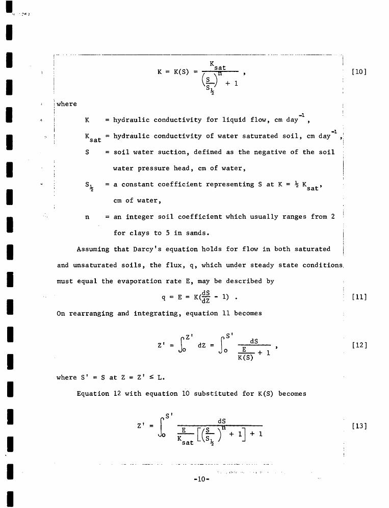
! K

K = K(S) K sat

-1 hydraulic conductivity for liquid flow, em day

-1 K = hydraulic conductivity of water saturated soil, em day ,;

1 sat :

S = soil water suction, defined as the negative of the soil

water pressure head, em of water,

a constant coefficient representing S at K = % Ksat'

em of water,

n = an integer soil coefficient which usually ranges from 2

for clays to 5 in sands.

Assuming that Darcy's equation holds for flow in both saturated

and unsaturated soils, the flux, q, which under steady state conditions.

must equal the evaporation rate E, may be described by

q = E = K(2§_ 1) dZ

On rearranging and integrating, equation 11 becomes

where S' = S at Z = Z' ~ L.

dS _E_+ 1 K(S)

Equation 12 with equation 10 substituted for K(S) becomes

+ 1

• \.:1''.' .• , . J i• \

-10-

[ 10]

[11]

[12]

[13]

I .. ~,:~


---·----·-·-----·--·--. -·· ··- ·---·-- .

The above integral can be expressed in closed form (Gardner, 1958).

·Equation 13 expresses explicitly Z' as a function of Sand E. It also

:defines implicitly the relation between E and S' for any given Z'.

!Both facts have been utilized in the past (Philip, 1957a and Gardner,

1958). However, utilization of the implicit relation is unwieldy in

·practice, except for n = 1 or 2. In the latter two cases the relation

;can easily be inverted and made explicit. In order to convert equation:

, 13 to a more tractable form, the following transformations may be

carried out. First, define the dimensionless variable,

e = E/K t' .sa

and substitute it into equation 13, obtaining

S' Z'=!J dS =

e o ( L) n + ( 1 + .!.) s-\ e

8' 1 r

e(l + ~) vo

Second, define a variable y by

y = 8/S~

= L (1:

( 1 + ~')~ 81: 2

1

e)n

and transform the integral of equa~ion 15 with its aid, obtaining,

after rearrangement, the basic equation of this study:

1 n s:· (e:

\ Z' di (e + 1) 1) -= 81: yn + 1 2

-11-

[14]

[15]

[16]

[17]


··-·-· .. -·--.. ---------·--------···---··1'"" - ..... -. ·····-·· -· _, ..

where y' = ~~ (e : lf

In particular, at the soil surface, when Z' = L

1

)n L yu

(e + 1) (e e I dl + 1 s~ = yn + 1

where 1 s l)n s~ C e

Yu = + 2

The integral on the right-hand side of equations 17 and 18 is

known in closed form for any positive n (Gradshteyn and Ryzhik, 1965,

equation 2.142). The form of equations 17 or 18 makes it possible to

determine the relation between e and the suction (either S' or S ) for u

any n by means of simple graphs. This technique as well as the ~esults:

obtained with its aid will be described presently.

For certain purposes, the use of equations 17 and 18 can be

further simplified by adopting the dimensionless variables

z z = s'

~

and t = L s , ~

-12-

[18]

[19]

[20]

[21]

I


in addition to the dimensionless e = E/K t used previously. With the sa

exception of s, these dimensionless variables are similar to those

·employed by Staley (cited by Anat, 1965) whose hydraulic conductivity

equation is also somewhat similar to equation 10. Inspection of

numerous curves indicates that S~ of the dimensionless s matches the 2

observed relations between K and S better than does the air entry

pressure, used in this connection by Staley. The above dimensionless

variables reduce the basic equation 18 to

1

I n s:u e

1) t dy

(e + 1) \e = + yn + 1

where

An analogous reduction can be carried out for equation 17.

The following reasoning leads to another useful relation which is

implied by equation 18. It is clear from physical considerations, that

an increase in the evaporative capacity of the atmosphere will produce

an increased suction at the soil surface. This higher suction, in

turn, must magnify"the upward water flux through the soil. If equation

18 correctly describes reality, such a flux cannot increase without

bound, because as S ~nd hence y ) approaches infinity, the integral on u u

the right-hand side of equation 18 approaches a finite limit, TI/(n sin*)

(Gradshteyn and Ryzhik, 1965, equation 3.241-2 with~= 1). It follows soil-limited

that a limiting soil water flux and hence aAli~ iti=s evaporation, e00

,

exists. For any particular soil system .. the ·latt,er is given hy

-13-

[22]

Is. t267


1

2

( e l)n L TI

(e(p + 1) e : - = ----CP sl.. n s-In !I. "2 .... n

3 or, in completely dimensionless form,

4

5-

6

7

8

9

10-

11

12

13

14

1 e n

(e(p + 1) (e : 1) t = CP

TI

n sin I!. n

The last two equations can be simplified considerably if e << 1 OJ

(that is, if E << Ksat).

and 24 lead to

In such a case, e + 1 ; 1, and equations 23 OJ

S n

[t J [ E ;; K CP sat

and

15- Equation 25 is similar to the formulas for EL. given without ~m.

16 derivation by Gardner (1958) for n 3 = 7 , 2, 3, 4 and yields identical

17 numerical coefficients.

18

19 APPLICATIONS

20- Data Required

21 The equations presented above may be used to compute the

22 estimated evaporation from bare soils under high water table

23 conditions. The data needed for such computations are as follows.

24

25·-

1!. S. GOVF:R!'iMENT PIUNTJNG OFFICE: 195'1 0- >11171

-14-

[23]

[24]

[25]

[26]'

19.1267


2

3

4

6

7

8

9

The meteorological data (those needed in connection with the

utilization of equations 4, 5 and 9) are obtained by standard

techniques or from references. These data include wind velocity, V , a

air temperature, T , the air relative humidity, h , and net radiation, a a

The magnitude of p(T )h , the water vapor pressure in the air, a a

is determined from T and h with the aid of standard tables or a a

formulas. Daily QN values may be determined either by direct

measurement, or by the method outlined in Slatyer and Mcilroy (Appendix

II, 1961). For a given site, the latter technique can produce

10- calculated QN values with the aid of standard information in the

11

12

13

14

Smithsonian Meteorological Tables (List, 1951). A zero value has been

assumed for Q in the computations of this paper. This is a reasonable g

assumption for daily means of Q , especially when these are used in g

conjunction with QN and· .A.P wE (see equation 9).

15- In addition to the above strictly meteorological data, the soil

16

17

18

19

surface temperature, T , is needed,. because it appears in equations 5 u

and 6. Data on this temperature are usually unavailable, hence the

need for the development of equation 9 as an indirect method for T u

determination. If however, soil surface temperature data are

20- available, it is possible to avoid the use of equation 9 and of the

21 usually approximate QN data needed in connection with this equation.

22

23

24

25·-

II. S. GOVERNMENT PHINTING OFFICE:: l'IS9 0- Sll171

867 • lOll

-15-


2

3

4

6

7

The soil equation requires knowledge of the hydraulic conductivity

for a reasonable range of soil water suctions. Such data will allow

evaluation of the necessary coefficients K t' n, and S~ for a sa 2

particular soil. K t can be measured directly and readily. sa However,

5- the other two coefficients are more difficult to obtain. They may be

computed from more routinely available data, using the technique of

!Marshall (1958), as modified by Millington and Quirk (1961) and by

Jackson and others (1965). This technique produces, for selected

9 magnitudes of s, a series of scaled hydraulic conductivity values

11

12

13

14

16

17

18

19

:.:·:J

:::'4

10 -· K' (S) = sK(S), where S is the scale factor and where K' (S) at S = 0 is

~0--

designated by K'sat• Note that the scale factor need not be determined K sat

to find n and s~. K' 2

If equation 10 is obeyed, a plot of log(K(S) - 1)

sat [= log(K'(S) - 1)] versus logS is linear. The slope of such a plot is

equal ton and the plot's intercept with the abscissa determines s~. 2

The manner of the computation of the scaled hydraulic conductivity

described in the above references. The basic

by these computations is the characteristic

relation between the soil water suction and t~e volumetric moisture

content (that is, the water retention curve or the pore size

distribution function). Such data are regularly determined in soil Some of these

laboratories. ~~may also be obtained in the field by measuring the sufficiently

moisture content of the soil overlying aAshallow water table as a

function of depth, after a prolonged period of negligible soil water

,,, I flux~s. --------·--------------------------------~------------------------~

II, S, GOVF.RNMI::NT PRINTING OFFICE:; 1'1'~? ll- C.lll ?I

867 ·lOll

-16-

Is. t267


Homogeneous Soil

2 For a homogeneous soil with insignificant vapor transfer

3 (figure 1, Case A), evaporation, E, can be computed from the

4

6

7

8

9

meteorological and soil equations in several ways. In most cases it is

5- convenient to compute e first. When appropriate, e may be converted to

E using equation 14. In the early stages of the computation, -the

soil-imposed upper bounds of e (e ) or the bounds imposed by 00

atmospheric factors (e t) may be needed. They can be easily computed po

as will be shown presently.

1o- Equations 4, 5, 6 and 9 are combined and yield an overall

11

12

13

14

16

17

18

19

meteorological equation, which expresses S as a function of e and u

which corresponds to equation 1. This equation is substituted into the

soil equation 18 yielding a nonlinear algebraic equation in e. The

root of this equation may be found by routine numerical methods. In

15- this study, the method of "false position" (Hildebrand, 1956, pp.

446-447) was programmed for a digital computer, tried, and found

satisfactory.

Alternately, e can be obtained by plotting the curves

corresponding to the above meteorological and soil equations, the

20--· magnitude of the actual e being· given by the intercept of the two

21

22

23

24

curves. The meteorological equation is plotted for selected values

of e < e in a straightforward manner. The soil curve is determined pot

for selected values of e < e using the following graphical procedure. 00

Any given e value may be used with an appropriate (that is, proper n)

"-~lot of

1!. S. GOVI·~IH:MENT !-'HINTING OFFICE: 14~9 0-511171

-17- 867•100

1.1287

I I I I I I I I I I I I I

2

3

4

6

7

8

1

(

,n f = f(e) = (e + 1) --!--).

e + 1

to determine the corresponding value off (figure 2). When f is

multiplied by t = L/S%,one obtains the magnitude of the left-hand side

~- of equation 18. This magnitude is equal to the value of the integral,-

. I = I(y ) , on the right-hand side of the same equation. Then by using \

I a plot :f I (y ) , given in figure 3, y. is found. Finally, the require~ I u u

I Su is computed from yu using the relevant definition, g·iven below

9 I equation 18.

10 _1 For less accurate but quicker estimates of the soil curve,

11

12

13

16

I . I dimensionless plots of the type illustrated in figures 4A and 4B may

I be used, the needed values of e and s being obtained for any given

z = t. The limited range covered by the plot, and the necessity for a

field filled with many curves are the obvious detriments of this

15 _1 approach. It should be noted that the curves in question also indicate

I the suction within the soil profile as a function of depth for any

11 given evaporation rate.

!8

!9

20-

I ,,

I I , .. ,. L.--------· ------------'-----I 1:. ~:. GOVI':H~~~VIl:NT i'Hii'ITINO OFFICi::: JQ~~ ll - ''i:! 71

-18-

I

[27]

I

I I I I· I I I I

f (e)

I I I I I I I

. 0 _ _.__..__...,__~.....___..-,---L......._,.,_____,....L.-----L-.----1..;.._,....&..;..;.---L-__,..l...;..---L.-----L..,-~, _j

0 5' 10 . 15

e x 105

I .!. n

Figure 2.--Dimensionless plots of f = f~e) = (e+l} ( e~l) for n ~ 2, 3, 4, 5 ..

I -19-

I

I

I I 0 -I an

II

I c 10

I .,; ~

..j"

~

M

~

I N

II c: )..j

0 .....

I ~c:: ::l

>. ·o c_ __

I :J II

0 ,-..

~ :l . >, - '-' .....

I II

......

..... 0

Cll .u

I 0 ...... c:l.

10 Cll Cll

• (11 ...... s::

I 0 ·~ Cll s:: (11

E ..... 0 I

I I

M'

(11 .... ::l

,bl)

·~

I t<..

I I L _j_

0 • 10 -• • • - ..........

I ::1 ~ ~ .......

I -20-

I

- -

I N ..... Ill I

-

z

-

30

20

10

- - - - - - - - - - - - - - .. r l

n=2

e =lx 10·1

e=lxlo·•

e=lx 10° L-----~----~----~~----~----~----~------~----~----~-----J

20 40 60 80 100 s

Figure 4A.--Dependence of dimensionless soil water suction, s, on dimensionless soil height z. The numbers labeling the curves indicate the magnitude of dimensionless evaporation rates, C'.

A. Soil parameter n = 2.

- -

I N t--4 cT I

-

z

-

20

10

0

- - - - - - - - - - - - - - -r I

n=5 e=lxlo-•

e=lxlo-•

e=lxlo-•

~~~~~=-~~~~~ 20 60 40 80 100

s Figure 4B.--Dependence of dimensionless soil water suction, s, on dimensionless soil height, z.

The numbers labeling the curves indicate the magnitude of dimensionless evaporation rates, e. R. Soil parameter n = 5.

19.1267


[~xact and approximate limiting evaporation rates, imposed by soil I ~

00 r E

00, can be obtained from equations 23 through 26, The

3 !approximate values are given directly by the appropriate equations.

• JThe exact values can be computed easily with the aid of figure 2, or

~-· jif less accurate values are needed, they can be read off directly from !

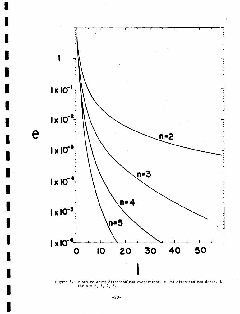
G an appropriate dimensionless plot in figure 5.

7

8

l~

13

14

lb

li'

!9

The limiting evaporation rates imposed by meteorological

conditions, e t' can be computed (graphically or numerically) for any po

weather data by solving simultaneously equations 5 and 9, with

10 .. h = 1. 0 (that is, with S = 0) • u u

Examples of results obtained with the aid of the above graphical

;methods are shown in figures 6, 7 I

and 8. The examples refer to two I

I selected soils, Chino clay with n = 2, s~ = 24, and K = 1.95 sat

: (Gardner and Fireman, 1958) and a coarse-textured alluvial soil taken I

~~-· j from the 50-60 em zone of the u.s. Geological Survey evaporation t~nks I I near Buckeye, Arizona, with n = 5, S~ = 44.7 and Ksat = 417. These

j evaporation tanks are described by van Hylckama (1966). I i I

I ... I

22

I I

L._ -. --·---·--- ····- -·------·-- _j

I. ~;. GOVI':ll!'.:.·,t:;:'ll'i l'iCINT!t-;G OVFJ-.'t': !•)· ·; ,, -~I: I:'!

H~'/•l·W

-22-

I

I I I I I I I I I I· I I I I I I I I

e

I

1 x lo·•---------.....___~____._-----~-.L.-__.__---'--~ 0 10 20 30 40 50

I Figure 5.--Plots relating dimensionless evaporation, e, to dimensionless depth, t,

for n = 2, 3, 4, 5.

-23-

.9.1287


2.

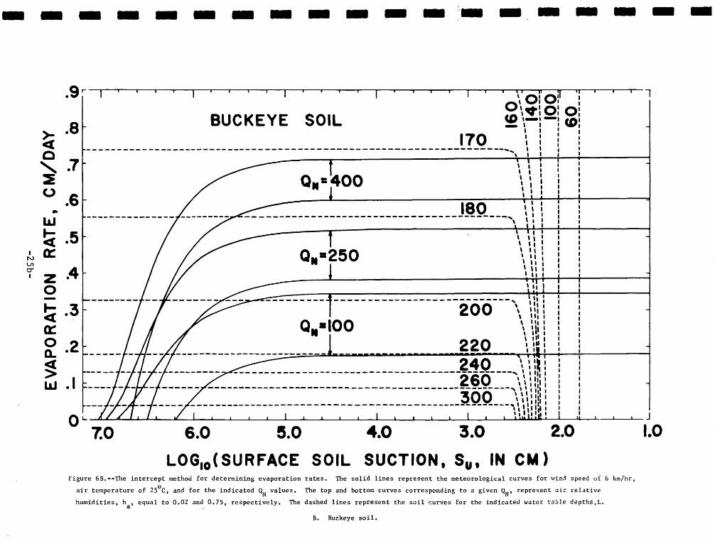
Application of the graphical intersection method is illustrated inl

figures 6A and 6B. Each figure shows meteorological curves for several

3 arbitrarily selected atmospheric conditions and soil curves

4 corresponding to several water table depths. Note that the soil curves

5- approach a limiting E with increasing S , in agreement with the u

6 previously presented theoretical proof. The rate of approach to the

7 actual E00

(or e00

) shown by the soil curves mainly depends on the value

a of n characterizing the particular soil. A relatively rapid approach

in 9 is exhibited by the Buckeye soil (n = 5) while

1the case of Chino clay

10··· (n 2) the approach is much more gradual. It should be noted that

11

12

13

14

16

17

18

19

~'1

22

most of the field soils commonly found show n values which lie between

2 and 5. Hence, such soils will usually yield E(S ) plots similar to u

or intermediate between those shown in figures 6A and 6B. The

meteorological curves also seem to approach a limiting E, but with

15·- decreasing S. The values of E, fixed by the intersection points

between meteorological and soil curves of the figur~s in question,

represent the actual evaporation rates under the particular

meteorological, soil and water table conditions.

20-

_______ j -24-

-

I N V1 IU I

- - - - - - - - - - - - - - - - -.9 !'"' I I I I I I I I I I I I I I I I I I I I I I I I I I I I I I 1

> .8 <I c '.7 ~

0 .6 .. l&J

~ .5 0:

z .4 0 -~ .3 0::: 0 0.. .2 ~ w .I

CHINO CLAY

--------.... .......... ,

o .. ·2so

----------------- 90 ................... -.....

',60 ' ' ' ' ' \

'

..........

120 ---------........

.... '

.........

' ' '

' \ \ \ \ \ \ \ \ \ \

OL

........ , -----......... ', ------ --.... \ J .... ', \

7.0 6.0 5.0 4.0 3.0 2.0

LOG 10 (SURFACE SOIL SUCTION, Su, IN CM) Figure 6A.--The intercept method for determining evaporation rates. The solid lines represent the meteorological curves for wind speed of 6 km/hr,

air/temperature of 25°C, and for the indicated QN values. The top and bottom curves corresponding to a given QN' represent air relative

humidities, ha, equal to 0.02 and 0.75, respectively. The dasred lines represent the soil curves for the indicated water table depths, L.

A. Chino clay.

1.0

..

- - - - - - - - - - - --- - - - - -g r I • 1 1

• I ' I ' ' I I I I I I ' I I i I I I I I \' I' :1 ij I I I 1.

O,o.o~ :

>- .8 <I c '.7 ~

0 .6 .. L&J

~ .5 ~ 0:: ll1

r z .4 0 -~ .3 0::

~ .2 ~ LaJ .I

BUCKEYE SOIL \•~ o: o: <D ,_, -· ,ft, -\ I I~

170 --------------------------------------------------------------~---,, \

180 --------------------------~-------------~, \

' ' ' \ I ' I ' I '

-------------------~()() ___ \ \

' \ 220 240 \ ~ :t

----------------------------------------------------------, \ I II 260 \\:~·: ----------------------------------------------------------"\\'II., 300 ,,.Ill,. \ I l I I I

OL ---------------------------------------------------- .. ,\I I I I~

'/ L 1 , ' I .1 1 I I I I 1 I I I I 1 I I I I , I , ~ \J l n I! : ' ~: I J

7.0 6.0 ~.0 4.0 3.0 2.0

LOG10 ( SURFACE SOIL SUCTION, Su, IN CM) Figure 6B.--TI1e intercept method for determining evaporation rates. The solid lines represent the meteorological curves for wind speed of 6 km/hr,

air temperature of 25°C, and for the indicated QN values. The top and bottom curves corresponding to a given QN' represent air relative

humidities, ha, equal to 0.02 and 0.75, respectively. The dashed lines represent the soil curves for the indicated water table depths,L.

B. Buckeye soil.

1.0

-

1-1287


2

3

4

6

7

8

9

The dependence of the actual E on weather and water table depth is

demonstrated more clearly in figures 7 and 8. Figure 7A and B is

concerned with the influence of the depth to water table under given

meteorological conditions. This figure demonstrates that for a

5- particular soil and meteorological condition, the evaporation rate

remains essentially constant and fixed by weather, if the water table

depth does not exceed a certain value. With the water table at

!greater depths, the evaporative flux decreases markedly because the

soil becomes the limiting factor. In other words, the flux decreases

11

12

13

10- because in figure 6, the pertinent meteorological curve intercepts the

!flat portion of the relevant soil curve. In agreement with the

observations by Philip (1957b}, for any given set of meteorological andl

soil conditions, the transition between the horizontal and descending

14 portions of an appropriate curve in figure 7 is so sharp that it can be

15-1 taken as discontinuous and its curvature can be neglected. Therefore,

16 each curve of figure 7 consists, essentially of a horizontal part

11 fixed by the weather, and a descending part fixed by equation 23 or 24

18

19

:·t

22

23

(that is, by figure 5).

It is this characteristic form of the curve that leads to the

20···!simplicity of the following procedure for determining the actual E ..

The appropriate soil-limited evaporation, E , may be determined with co

!equation 23 or 24, and plotted against depth to the water table.. The

appropriate meteorologically controlled potential evaporation, Epot'

24 I

, I __ --·- . ....... -·-·- -------·-··· -----·---·--· -----· -----------·---· -···--·--·-·-·-- .

.. 26-

I I I I I I I I I I I I I I I I I I I

~ .8r ,

c

' .7 -. \

2 \ CHINO CLAY a.·40o, u .6 \

\ .. \ LIJ \

~ .5 \ \ \ a:: \

z A \ \

0 \ - \

~ .3 \ \ a::

0 a. ~ 1&.1

Q••IOO \ \

.2 \ ~ ~ ~ ~

.I ~

.L--------~----------L---------~-------------------~

0 100 200

DEPTH TO WATER TABLE, CM Figure 7A.--Relation between evaporation rates and water table depths,

calculated by the intersection method (solid lines). The indicated meteorological conditions are identical with those of figure 6. The descending solid line also represents the exact soil-limited rates of evaporation obtained from equation 23. The dashed line represents the approximate soil limited rates of evaporation and is obtained from equation 25. The exact and approximate curves coincide in B.

A. Chino clay.

-27a-

- - - - -.8r

> g .7

' ~ .6 ..

1&.1

~ a: 4

• z I

2 .3 N -....J

1-0' I

C( a: .2 0 Q. c .I > 1&.1

OL 0

- - - - - - - - - -• -------y- .-------T T --- ~ ~- --. -~-- -. ----------. r --------. ---.-- ,

a,.~4oo

Q,.•250

Q,.ciOO

BUCKEYE SOIL

--~----~----~--~-----L----~--~-----L----L---~----~----L---~-----L----~--~

100 200 300

DE-PTH TO WATER TABLE, CM Figure 7B.--Relation between evaporation rates and water table depths,

calculated by the intersection method (solid lines). The indicated meteorological conditions are identical with those of figure 6. ;he descending solid line also represents the exact soil-limited rates of evaporation obtained from equation 23. 1be dashed line represents the approximate soil limited rates of evaporation and is obtained from equation 25. The exact and approximate curves coincide in B.

B. Buckeye soil.

- - - ..

1.1267


2

3

4

-----------

may then be entered as a straight, horizontal line. The actual

~~~~~~D evaporation for any given water-table depth may be taken as

the lowermost portions of the two intersecting curves.

Note that if E << Ksat' as in the case illustrated in figure 7B,

s- the exact and approximate E curves essentially coincide. Hence, (X)

6 equations 25 or 26 may be used for estimating E under such circum-

l

On the other hand, figure 7A illustrates a case in which

does not occur. As a result, the approximate E

such I curve

7 stanceso I Ia coincidence

I 8

9

10-

~ :

12

13

14

15

(X)

!overestimates the actual E in the descending portion of the E curve.

Figure 8 illustrates, for several water table depths in Chino

soil how efficiently the atmosphere can remove soil water under

various meteorological conditions. The index of the meteorological

conditions is the potential (that is, S = 0) evaporation, E t• The u po

efficiency of removal is measured by the ration E/E t• For a given po

water table depth, the figure demonstrates that the maximum efficiency

i I

I I

16 of water removal (= 1.0) occurs at small values of Epot For any given

I 7

J8

water table depth, as E t increases, the efficiency remains at a po

maximum until a certain limiting E t is reached. Thereupon the po

t9 efficiency declines rapidly. This transition point is fixed by the

.'!I water table depth and occurs when the evaporation rate becomes limited

by the soil's inability to conduct water rapidly enough.

~·· -- .. ·--·--------------------~--·---- ---·--------·--- --· ··---·- ._...,_._.

-28-

\ i I I

I

I J

-------------------

I N \.0 I

L1J

~ "0:: 1.0 Wz ~2 0::~

<(

zo::: 2 ~ .5 ~~ 0::~ 0 o....J CHINO CLAY

I 180

~~ wlz

0 . .2 .4 .6 .8

lU 1- POTENTIAL EVAPORATION RATE, CM/DAY 0 Q.

Figure 8.--The dependence of relative evaporation rates, E/E , upon the potential evaporation rates, E , for pot pot Chino clay. Numbers labeling the curv~~ inJicate the depths to water table.

1-1287


Layered Soil

2 In a manner analogous to the homogeneous case, steady state

3 evaporation in a layered system unaffected by vapor transfer may be

4 described by the functional relations appropriate to each layer.

5-· For a soil with i layers above the water table, (figure 1, Case B),

6

7

a·

9

10-

11

12

13

14

15-

16

these relations may be symbolized by

Soil layer 1 (lowermost) : I;. = F (Sl ' E)' -~

Soil layer 2 ~ = F (Sl ' Sa' E)' 8:a

E)' Soil layer 3 La = F (Sa ' Ss ' &3

Soil layer i (uppermost) : L = Fg (Si-l , S , E), u i -· u

The atmosphere E = F (S ). m u In any one of the equations 28-j above (j = 1,2, ••• i), S.

1 and

J-are,

s.~respectively, the suctions at the lower and upper interface of J 1\.

layer j. Note that S is known (S = 0). 0 0

Therefore, it does not

appear in equation 28-1. In addition, in conformance with the earlier

11 symbolism, Si ~is designated as Su (see equation 28-i). Presently,

1a the subscript j will also be used for subscripting the coefficients n,

19 S1: and K t of the layer j. 2 sa

20- The above set of equations may be solved simultaneously since it

:-?1 contains as many equations as unknowns. Such a solution may be

22 achieved using either a numerical or graphical (intercept) method.

23

24

The latter method will be described presently. Note that, as in the

2:.; interface.

the present approach is possible due to the fact

layers exhibit identical suctions at their common lhomogeneous case,

that two adjacent

··---·· -·--·-------------------------------l

-30-

ll. S. GOVERNMENT !'HINTING OFFICI':: 1'1~9 (J-<;11111

8~7 ·IOU

[28-1]

[28-2]

[28-3]

[28-i]

[29]

I ... t,


It will be recalled that the intercept method discussed

previously involves finding the intersection between plots

~epresenting the meteorological and soil equations. In applying the

intercept method to the layered case, one must deal with diffeuen~ sets which differ from layer to layer

·of parameterA. Hence, E and s should be plotted rather than their

dimensionless counterparts, although e may be employed in certain

computations involving single layers. with the aid of

The meteorological curve needed is plottedA~equations

4, 5, 6 and 9, as it was in the homogeneous soil case. The graph that is

of the soil equation involves S (in addition to E), ~' the surface u

suction of the uppermost layer. To plot such a graph for a layered

soil system, a procedure for obtaining S from any given E must be u

used. This procedure involves the determination, for a given E value, ,s j'

of the suction~at the upper surface of each successive soil layer,

starting with j = 1 and ending with the ·appropriate value of

S for j = i. u

The equation for computing such a suction at the lowermost

layer 1, (figure 1 Case B), is:

dy

yi1. + 1

where

-31-

[30]

I I I I I I I I I I I I I I I I I I I

with Note that equation 30 is identical~~·equation 18, because of the

physical similarity of the respective situations. The graphical

procedure for obtaining sl (utilizing figures 2 and 3) described for

equation 18 is applicable here.

In the second step, the following equation is used for the

relations in layer 2:

1

( e2 1)~. ~

(ea + 1) e2 + -(S ) = !:- 2 2

1 ' [31]

where e2 = E/ (K t)2 sa

1 82 e2 ~

y2 = (S!:-)2 (e2 + 1)

2

1

sl e2 na

}\ = (S~)2 (e2

+ 1)

-32-

I


The derivation of the above equation is identical in principle to that

of equation 17. However, the lower boundary condition here is S = S l

and not zero, as it was in equation 17.

Equation 31, for ease in handling, is rearranged:

~ -+ (S~)2

dy

y~ + 1

With the aid of equation 32 one can find S2 for the given S1 and E

values. To accomplish this, first compute y1 and e2 , using the

relevant definitions given in Gonnection with equation 31. The

integral~ on the left~hand side of equation 32, I(y1 ) is then

evaluated employing the appropriate cu~ve of figure 3. Next, a

technique identical with that of the homogeneous.case (and involving

figure 2) is used to determine.the magnitude of the first term of

equation 32, f(e2 ) 1;a /(S.!>) 2 • Addition of the latter term to the 2

previously computed l(y1 ) yields the value of I(y2 ) from which S2 i~

computed using figure 3. such as

Equations~~ equation 32, with subscript 2 replaced by

j = 3,4, ••• i, may be written for each ~dditional soil layer. Thus the

calculation procedure may be carried stepwise up the soil profile. the

The equation for the uppermost layer, leading t~Su values sougqt is:

1

-33-

[32]

[33]

I


with the definitions of y, 1 andy similar to those of analogous terms 1.- u

in equation 31. only

Often, theAinformation sought is ~the dependence of the

soil-limited evaporation, E , upon the water table depth. Such CX)

information may be obtained for multilayered systems without determining

the individual soil curve and without using graphical or numerical

means. Most of the required procedure consists of computing, for

various E values of interest, the suctions at the lower surfaces of

successive soil layers, starting with the uppermost layer, i, and

finishing with the layer just above the one in which the water table

can be found. These computations are followed by calculation of the

water table position in the lowest soil layer, 1. required by such a proced~re

The i'BlB 8ft@ equation for the uppermost layerAis derived from

equation 33, by noting that e is associated with an infinite S and CX) u

hence with an infinite y • This in turn implies that the integral on u

the right of equation 33 is equal to TI/[n. sin (TI/n.)] (see the 1. 1.

derivation of equation 23). Using this fact,one obtains, after

rearrangement, the following equation for the uppermost layer:

n u

-34-

dy

y~ + 1 [34]

19.1267


The value of the left-hand side of equation 34 can be computed for the

2 known parameters involved. From this value, y 1 is determined with u-

3 the aid of figure 3. The definition of y 1 provides the means of u-

4 calculating the corresponding S. 1

• 1.-

5- The underlying layers, j = i-1, i-2, ••• ,2, are described by

6 equations identical in form to equation 32, but with index 2 replaced

8

9

by indices appropriate to the particular layer. These equations may

be successively solved for S. 1 , progressing downwards, in the manner J-

closely resembling the one described in the preceding paragraph. In

10- each step, the suction previously determined at the lower interface

11

12

13

14

16

17

18

!9

;'1

22

24

provides the suction value for the upper-interface of the analyzed

I layer. This procedure may be carried out stepwise, down the soil

·profile, for any number of discrete soil layers, until the lowermost

layer is reached. At this point, equation 30 is used with y1

known

15- from the solution of the equation appropriate to the layer just above.

This equation is applicable because the suction at the lower surface o

layer 1 (the water table surface) is equal to zero for all cases.

!Equation 30 may be used for determining the value of~ which

corresponds to the value of E employed. The final result of such a

?o-- computation for a given value of E is the relevant depth to the water

2h .

table expressed as the sum total of soil layer thicknesses. Note that

as computations for various E values progress, the water table position

may be found to shift from one soil layer to an adjacent one. Such

cases would necessitate an appropriate adjustment in the computation

p~ocedure outlined abo_v_e __ ·------------------~--------------------

-35-ll. ~. 00Vf:l!r01E:'I:T 1-'HINTIJI,;G OFFICI;: J';IS'I n--~11171

867 -ton

19.1267


2

3

4

6

9

r

I Figure 9 demonstrates the application of either of the above two

I computation methods to Buckeye soil with: i. no crust; ii. the same

I soil overlain by a slightly salt-cemented upper crust

(n = 4, S% = 28.1, Ksat = 47) of either 3 or 10 em thickness; and

~i-· iii. the same soil overlain by the 10 em crust of the previous layer

plus an uppermost 10 em layer of a hypothetical soil (n = 3, S~ = 20, 2

K = 20) The figure· shows clearly that a relatively thin less sat •

permeable layer may markedly decrease evaporation rates.

Effects of Vapor Transfer

10- If a homogeneous soil in contact with a water table is suf-

l!

12

14

lfi

I J

td

:'I

.·· ~

ficiently dry near the surface, water transfer in the dessicated,

upper region involves primarily vapor rather than liquid flow. Vapor

flux in this layer may depend significantly on soil-temperature

gradients. The probable existence of such a transfer can be detected

I

lb·! by noting that, in general, appreciable vapor-transfer influences in

soils tend to occur when h ~ 0.8 (Philip and de Vries, 1957;

Rose, 1963b; Jackson, 1964). To utilize this fact, derive h , using u

the previously described procedures for cases unaffected by vapor-

I transfer (for example, after computing E, employ equation 5 to

~()-- evaluate h ) • If the derived h value is smaller than 0.8, it might u u

be expected that E can be significantly affected by vapor-transfer.

I

l ...... . '"··-··--·-·-····---··---------'-----_j

-36-

1:. !>. GUV,:Ho\o:"S:-.lT I"HINTlNG OFFI~·l;: ~~··~ 0 • ;lli71

tl6 7 ·11J•'

- - - -

I \.t.J -...,J

I

- - - - - - - - - --- -~ .8r , C( c '.7 t 2 QN1400 0 .6 \:jm\ BUCKEYE .. SOIL w ~ .5t l a: a.=25o z .4 1 0

'\ \\ .. La=O - l ~ .3 a. =loo / 0::

~ .2 1 ~ L&J .I

OL ~

0 100 200 300 400 Figure 9.--The influence of layering on the relation between evaporation rate and depth to water table.

Soil evaporation limiting curves are shown for i. the homogeneous case(~= 0); ii. a two-layered

soil, with the upper layer thickness, Le, of either 3 or 10 em; and iii. a three-layered soil with

thethicknesses of intermediate and uppermost layers equal to Le = 10 em and ~ = 10 em, respectively.

- - ..

19.1267


When the dessicated, upper layer in question is present, ·a more

2 or less exact evaluation of E involves numerical integrations and is

3 based on heat-transfer as well as water-transfer equations. The

4 approach outlined below avoids this relatively complex procedure, but

5-- it is clearly approximate. This approach utilizes a suggestion

6 originally made by Gardner (1958) and a theory of vapor-transfer in

7 soils developed by Philip and de Vries (1957; see also de Vries, 1958)

8 Gardner suggested that the homogeneous soil-water system in

9 question may be represented approximately by a two-layered column

1o- (figure 1, Case C) in which water is being transported exclusively in

11

12

13

14

16

17

18

!9

23

vapor form within the upper layer u, while in the lower layer 1 only

liquid flow take place. The theory of Philip and de Vries (1957),

applied to the dry, upper soil layer of such a system may be formulate

in terms of humidity and temperature gradients. Such a formulation

15-J results in the following equation of vapor flow

where

20·-

E = _ D dh _ D dT hv dz Tv dz

Dhv = a coefficient characterizing the molecular diffusion of

a -1 soil-water vapor caused by humidity gradients, em day

DTv = a coefficient characterizing the molecular diffusion of

soil-water vapor caused by thermal gradients,

a -1 o -1 em day K

.J4 It can be shown (Penman, 1940, Philip and de Vries, 1957) that the

,; ~e~~icient Dhv __ 1_·s __ d_e __ s_c_r_i_b_e_d __ b_y-------------------------------~--------~ -38-

1'. !:i. GOVI;:R!'>:·•~:NT i'klNTING OFFICE;: !Q~'! 0- ··.1 1111

Ho7• lOll

[35]


2 where

3

4

5-

6

7

8

9

10--

11

12

13

D = a coefficient characterizing the molecular diffusion a

a -1 of water vapor in free air, em day

ao3 = 50.91 T /P, (de Vries, 1958),

p = ambient pressure, mb,

cr = volumetric air content of the soil, dimensionless,

~{cr) = a dimensionless function defining the effectiveness

of the water-free pore space for diffusion

,... a,cr,

a = tortuosity factor, dimensionless ~ 0.66,

p = p (T) v v

-3 = density of saturated water vapor, gm em

P is a function of temperature. v

14 According to the Philip and de Vries theory, the coefficient DTv

15- is given by

16 D ~ fP/[P- hp(T)]} (dp /dT) C h/p , a v w

17 where

18 ~ = soil porosity, dimensionless,

19 C = a ratio of the average temperature gradient in the air-filled

21.)- soil pores to the overall soil temperature gradient; this

21 ratio depends upon soil porosity, water content, temperature

22 and quartz content; it usually varies between 1.3 and 2.3,

23 except in extremely dry, compact soils in which it may reach ,

24 the value of 3.2, especially if the soil contains much quartz

;>') ·- (see Philip and de Vries, 1957, and Rose, 1968),

11, ~. GOVERNMI::NT !-'HINTING OFFICE: 19'i<l 0- 5111:1

•39- 8i:?•ICO

[36]

[37]

1-1267


2

3

4

5-

6

8

9

Note that

where

DTv = Bh Dhv ,

B = en /cr) ('/a) [ d (loge p v) I d T] = en /0') ('/a) a ' , gm em-s °K -l

.... -4 S' = d(log P )/dT = 0.1516- 3.22 x 10 T; the latter empirical e v

equation has been fitted for 290°K < T < 360°K using data from List (1951).

It follows from the expressions for Dhv and DTv given above, that

equation 35.can be written

E --- =

Dhv dh + Bh dT dz dz

10- Utilization of equation 39 is facilitated by the following

11 approximations, which are made possible by the low water content of

12 the upper soil layer in question.

13 First,in dry soils, the volumetric air content, cr, is

14 approximately constant and equal either to porosity, ~, less the water

15- 1 content of air-dry soil, or to~ alone, if the latter water content is

16 negligible. Hence the ratio ~/cr of B is approximately constant and

11 often equal to unity. It may be noted that of the other factors

18 determining B, only C depends on variables other than temperature. In

19 this study C, which in all soils is of the same general order of

20-- magnitude, will be taken as a constant and all the computations needed

for determining E will be carried out twice: once for the probable

.... minimum value of C, (C 1.3) and another time for the corresponding .,..,

.. r

maximum value (C ~ 2.3). It can be shown that such calculations lead j 1

to the estimation of the probable upper and lower bounds of the E valu

? 4 ! sought. It follows from the above considerations that in this study i

., I will be possible to regard B as determined by temperature alone. _j .:,.) . !_ ___________________________________________ _

-40-

[38]

[39]

I I I I I I I I I I I I I I I I I

2

3

4

Second, in dry soils, the ratio P/[P- hp (T)] is approximately

equal to unity. Hence, the coefficient Dhv of equation 39 can be

regarded as a function of temperature alone.

In addition to the above approximations and to soil and

5- meteorological data, needed in the previously discussed cases, the

6

7

8

9

10-

11

12

13

14

15-

16

17

18

19

20-

22

23

24

approach under consideration requires two new assumptions, as well as

acquisition of information about soil temperature, ~, at one small

* depth, L • The latter depth is defined here as one which may exhibit u

a significant gradient of the mean daily temperature. In the

computations of this study, the L* value was taken as 2 em. u

'Ihe first new assumption required is that the temperature gra~lient

in the dessicated, L em deep, upper layer does not vary with depth u

* and is approximately equal to (T - 1' )/L • u ., u

The second new premise is based on the fact that Dhv and B,

though temperature-dependent, do not vary greatly with T. Due to this,

the following can be assumed for temperature ranges commonly met near

the soil surface: Dhv amd B are independent of temperature, if they

are evaluated at the mean temperature of the upper soil layer defined

It will be noted that the above two premises tend to imply that

the depth of the upper layer in question, L , is not very different u

., ... from L'. If the procedure to be derived presently yields results whic

u

are strongly at variance with this implied assumption, a satisfactory

assessment of E may require certain special measures. These will be

described in due course.·

-41-

II, S, GOV~:RNMENT PHINTING OFFICE: 1959 0-511111

867 •IOU

1.1287

I I With the aid of the above approximations and premises, equation

I 2 39 can be easily integrated. ·First, this equation is rewritten in a

3 slightly different form,

I 4

I I I I I I I I I I I I I I

5 --

6

7

8

9

10-

11

13

14

15·-

16

1 7

18

19

dh c d; = b(h - 1)) '

where

c = E/Dhv •

Second, h of equation 40 is replaced by a new variable,~' defined by

~ = h- (c/b). The resulting equation in~ is readily solved by

separation of variables, using boundary conditions, which state that

the variable h assumes the values of h and h at Z = (L - L ) and .). u u

Z = L, respectively. This solution yields, after rearrangement, the

working equation of the procedure under consideration

L u

h (c/b) 2.3 1 u = b 0~ o _.~~-(-c-=-/b~) •

Equation 41 makes it possible to compute L for a given E, if the u

relevant soil properties are k~own, and if the given value of E is

22 plausible under the assumptions made. Note that because of the latter

23 limitation, when b is positive (that is, when Tu < ~), ~here w;i.ll

24 exist certain arbitrarily chosen E values for which equat;i.on 41 cannot

2 ~ __ yield a meaningful answer.

-42- &ti"i• IV·

[40]

[41]

19-1267


The value of ~ in equation 41 may be taken as corresponding to

2 the soil moisture suction at which the vapor transfer influences

3 become sufficiently important. According to theoretical considerations

4 of Philip and de Vries (1957) and measurements by Rose (1963b), liquid

5- flow commences at h ~ 0.6. Jackson's experiments (1964) suggest for

6 desorption that this value may lie between 0.5 and 0.8. The

7 commencement of appreciable vapor-transfer influences probably occurs

8 at somewhat higher values of h than those associated with the

9 commencement of liquid flow. Hence, perhaps \ could be taken as at

IO-· least equal to 0. 8. For a given soil, the soundness of this choice can

11

I 12

13

14

1">·-

16 I

17

18

19

be checked and possibly improved by comparing the value of K = Kl. ~q

at

h = 0.8 (computed with the aid of equations 6 and 10) and the value of

the corresponding coefficient of isothermal vapor transfer (Rose,

1963a), K = (Mgh Dh ) I (RT). If K ~ K1 . , it is very probable vap v vap ~q

that the value of ~ chosen was suitable.

Whichever reasonable value of ~ is used, it is found that the

interface suction S1

, which corresponds to ~ , is relatively high

and usually exceeds 10,0~0 em. For suctions of this magnitude the rate

of water flow in the moist soil below the interface in question is

20 ·- essentially soil limited. Hence, the rate of water transfer in the

2''

23

24

lower, moist soil layer can be evaluated with the aid of equation 23.

If the thickness of the moist layer is taken as ~ = L - Lu, then for

steady state conditions and any given L, equation 23 (with its L

!replaced by L - Lu) in effect expresses E as an increasing function of I

,., Lt:h~_~_ry l~yer <Jepth, L _j l'. '>. GOVEI!SME~~T I'HINT!Nl~ ll!o'FJ('f:: · 1'6~ ". ···ill71

t'ci7 ·1011

-43-

I

19-1287


2

3

4

5-

6

7

8

9

10-

11

12

13

14

15-

16

17

18

19

20·-

21

22

23

24

25-

Another relation,giving E as a decreasing function of L is u

expressed by the just derived equation 41. The two equations linking

E and L, (equations 23 and 41), can be solved simultaneously, either u

graphically or numerically, yielding the actual E and L • u

If the value of L thus obtained is of a different order u * .

should magnitude than L , the actual E which corresponds to L u u

reassessed. * If L << L , it might be u u desirable to acquire·new

of

be

r,_ data

for an appropriately small L* and to repeat the original procedure, u

using the new T,_ • On the other hand, if L >> L*, it is advisable to u u

consider the upper layer, u, as consisting of two sublayers. In the

upper sublayer, nonisothermal vapor tr~nsfer can be taken as the

predominant manner of water transfer. Equation 41 describes the

relevant relations for such a region. If the depth of this sublayer

is assumed to beL: and if E is given, humidity, 1\~, at the bottom

of the sublayer in question can be computed, since it follows from

equation 41 that

!\= (c/b) + [h - (c/b)]/exp(-bL*) u u

In the lower part of layer u, isothermal vapor transfer can be assumed

to be the dominant mode of water flow. Such a flow is described by

equation 35, with dT/dz = 0. Integration of this equation, leads to

the relation

L' = (h - h ~~) I (E /D ) u ·~ ·~ hv

in which L~ is the depth of the lower sqp}~Si:\"~MENT I'IHNTrNc oFFICE: 19s9 o- s11111

867 ·100

-44-

[42]

[43]

19-1267


2

3

4

6

7

8

9

For a given E, the reassessment procedure just outlined can

produce a corresponding value of L (= 1 1 + 1* ). Thus, a relation u u u

between E and L can be obtained for a set of arbitrarily selecte·d E u

values. As in the first vapor-case procedure described above, such a

5-- relation can be used in conjunction with equation 23 in order to

determine, either graphically or numerically, the desired values of the

actual E and L • u

The above procedures for including vapor-transfer in the

evaporation computations were tried out with the data of the Buckeye

10- soil on hand, and several estimated ~ values. The results obtained

11 showed that under the conditions tested (Tu > ~), the E value was

12 somewhat increased by the vapor-transfer influences. However, this

13 increase did not exceed 0.01 em/day (less than five percent of E) and

14 hence could be neglected for most practical purposes (compare with the

15- results of Hanks and Gardner, 1965). The reason for so slight an

16 increase probably was two-fold. Firstly, the values of Dhv and DTv are

11 rather small. Secondly, when Tu > ~ , thermal transfer is counteractin

18 the influence of the humidity gradients. If, contrary to the above

19 experience, conditions are such that significant vapor-transfer effects

20- are suspected, the methods given in this section can be used to estimat

21 such influences.

22

1 23

24 I

I 25-- ________ j t:. S, GOVEHN:-1F:NT !'HINTING OFFICE: 1<159 0- 51117i

I -45-

I

19-1267


DISCUSSION, EXPERIMENTAL TEST AND CONCLUSIONS

2 Of the relations which can be computed with the aid of the

3 approach presented in the preceding pages, the one which might be most

4 useful in hydrologic practice is described by the plots of E versus L,

5 _ as those in figures 7 and 9. A summary of the procedure based on using

6 these plots is given in the Appendix. The results obtained in this

7 study confirm Philip's (1957b) contention that for all practical

8 purposes, plots of this kind can be prepared by assuming that, for any

9 given L, the actual E(L) is the smaller of Epot and E~(L). In such

10- cases, the latter two quantities may be calculated, respectively, with

p the aid of the appr~iate meteorological and soil equations. It 11

12

13

14

16

17

18

19

21

22

23

24

follows that the actual E is either atmosphere-limited or soil-limited.

This implies that the region on the E(L) plots in which both

atmospheric and soil factors are influential is so small that it can

15- be neglected. For a Yolo light clay, Philip noted that the impreciseness

due to such a

than could be

experience of

was similar.

20-

25-

neglect as compared with the exact solution was smaller

exhibited on a graph bf the scale he used. The

this study, in which two very different soils were used,

-46-

U, S, GOVERNMENT !-'HINTING OFFIC'E: 1959 0- ~11171

867. 100


2

3

4

·6

7

8

9

The reason for the narrowness of this region of imprecision is

suggested by the shapes of the curves shown in figures 6A and 6B. An

inspection of these curves reveals that the S axis may be divided into u

the following three regions: (1) a low suction region (roughly

3 5- S < 6 x 10 ) in which the soil curves may show relatively steep slopes

u 0

but the meteortogic~l curves are nearly horizontal and are fixed by

E ;;.. E ; (2) an intermediate suction region (approximately, pot

6 x 103 < S < 6 x 104) in which soil and meteorological curves are

u

10-

·nearly horizontal and approach their respective, limiting E values;

(3) a high suction region (S > 6 x 104) in which the meteorological u

11

12

13

14

curves exhibit appreciable slopes, whereas the soil curves are

practically horizontal and are fixed by E ; E • From the above it is (X)

clear that an intersection between meteorological and soil curves which

occurs in the low-suction range results in E = E t• On the other hand po

15- when such an intersection occurs on the high-suction range, one obtains

16 · E ~ E • The intersections which occur in the intermediate range involv~ (X)

17 plots with nearly horizontal slopes of opposite sign. Hence, for any

18

19

21

22

23

24

given set of weather and soil parameters only a limited range of water

table depths will produce intersection values confined to the

20- intermediate S range. u

In this range the values of E may vary somewhat

the However 'A almost horizontal character of the curves specifies that the

actual value of E lies between the very nearly equal values of E t and po E~· Therefore, for all practical purposes, E ~ E t ~ E for the ...,.. po (X)

intermediate range. It follows from the above considerations that in

all three suction ranges in question, the actual E must be almost equal

25- either to E(X) or to E00

t or to both of these quantities.

-47-

ll. S. GOVERNMENT PHINTING OFFICE: 1959 0- Slll71

867 ·ICU

1-1287


2

3

4

6

7

8

It should be noted that the conclusion just stated very probably

is not restricted to the soil and weather conditions treated in the

examples of this study and that it can be expected to be applicable

rather generally. The reasons for this are as follows. Equation 3

5- demonstrates that the meteorologically determined E is a linear

function of h • However, it follows from equation 6 that u

h = exp [(-MgS )/(RT)] = exp [J..L2

x 10-7 S ] where Jl2 < 8 for the u u u u

commonly found surface soil temperatures, T • Hence, h deviates .U U

9 appreciably from 1.0 (that is, from full saturation) only if the S u

10- value is very high. 0

This accounts for the fact that the met~rological

11 curve deviates from the horizontal only in the high S range. On the u

it follows from _, 12 other handY\ equation 22 and figure 3 4Ja .. aa6il'at;e that for the usual

13 soil parameters and evaporation rates, the soil curves almost reach

14 their limiting level when S is still relatively low. This accounts u

15- for the soil curve contribution to the peculiarities of the E(L)

16 relation under consideration.

17

18

19

20-

21

22

1 23

24

I I I

25-

-48-

U, S, GOVERNMENT PHINTING OFFICE: 1959 0-~11171

867 ·I•JO


2

3

4

6

7

8

9

An inspection of figures 6A and 6B indicates that in the

intermediate suction range, the E(S ) curves drawn for soils with low u

valued n parameters (for example, n = 2) show the largest slopes,

whereas the soils with large n values (for example, n = 5) exhibit

5- the smallest slopes. Further confirmation of this conclusion is

It follows f~om implied by the curves of figure 3.A such a conclusion iapliiB that in

the intermediate ,suction zone, the lower the value of n, the larger

the limited range of transitional E values which depend on both soil

and meteorological factors. This might suggest that the E(L) estimatio

10- procedure under consideration is least precise in cases of soils with

II low values of n. However, even in these cases the procedure was found

12 sufficiently accurate for most practical purposes. Note also that the

13 appreciably sloping parts of the soil and meteorological curves shift

14 towards the intermediate suction region.as the limiting E values

15- decrease. Hence, the relative importance of the transitional E range

16 increases as the magnitude of the limiting E decreases. But for these

17 small values of E, the absolute importance of any imprecision of E in

18 the intermediate suction range is insignificant.

19 In order to test in a preliminary way the applicability of the

2I

22

23

24

20~ E(L) estimation procedure considered above,its results were compared

25-

with actual field observations. The field d~ta were obtained from two

large, bare-soil evaporation tanks located at Buckeye, Arizona and

described by van Hylckama (1966). The local soil contained in these

tanks had a slightly salt-cemented upper layer (layer 2 discussed

above in the la ered soil case) that a than 10 em.

-49-

eared to be somewhat thicker

U.S. GOVERNMENT PHINTING OFFICE: 1q59 0-511171

867.100

I I I I I I I I I I I

.The tanks were provided with apparatus for automatically

2 ·maintaining a pre•selected water table depth, and for recording the

3 quantity of water required to do this. Consequently, data on the

4 actual daily rate 9f evporation for a selected depth to water table was

5- readily obtained.

6 Meteorological' data, which. included air temperatures, air relative

7 humidities, and wind velocities, were also collected hourly at the

8 site. These variables, converted to a daily average basis, along with

9 tabular radiation data appropriate to the site (List, 1951), were

1o- used to calculate E t by the methods described earlier in this paper. . po

11 In addition to the above, soil temperatures at ·the depths of 5 and 10

12 em were recorded.

13

14

16

17

Data sets of various periods were chosen for analysis, primarily

on the basis of completeness of both actual E and E t information, po

15- and achievement of a steady state. All these sets were selected from

March to October data of three consecutive years.

1 18

19

I 20-

I 21

22

1 23

24

I 25~·-

I I

-so-

ll. S. GOVERNMENT PHINTING OFFICE: 1959 0 ~51 II 71

867 •IOU

1-1287

I I I

2

3

I 4

I 6

I 7

8

I 9

To provide information needed for calculation of.E00

, undisturbed

soil cores were obtained from the evaporation tanks at 0-10 em a'Q.d

50-60 em depths. The cores, 3 em thick. and ~ em in diameter, were

taken in successive, spaced pairs from each depth zone with a soil

5- sampler provided with retainer rings. Using the local ground water of

the area, saturated hydraulic conductivities and moisture retention

curves were determined on cores selected from the two layers. Each

moisture retention curve was determined in two parts. A ceramic plate

with a hanging water column was utilized for the 0 to 0.1 bar suction

a 10- range, whereas a pressure plate appax;{us (Richards, 1954, .Method 32)

I 11

12

I 13

I 14

I 16

17

I 18

I 19

I 21

22

1 23

24

I I I

was used for suctions between 0.1 and 1.0 bar. The moisture

retention curves for the two soil zones were used to compute the

appropriate n and S~ parameters by the methods described earlier ·in 2

this report. 'Ibese parameters we·re then used, along with the K t sa

15- data, to calculate E by the procedure outlined in the section of this 00

paper concerned with layered soil.

20-

25·-

-51-

ll. S. GOVEilNMENT !'HINTING OFFICE: 19~~ 0 ~ 511171

867 •lOll

1-1287


A comparison of the observed evaporation rates with calculated

2 E and E t is illustrated in figure 10. The circles on the plot co po

3 indicate average observed evaporation rates for three depths to water

4 table. Due to the insufficiency of the available data, these averages

s- do not carry the same weight. The circles, indicating the 120, 146,

• I and 156 em depths, represent the averages from 55, 13, and 6 days,

7 I respectively, The bars connected in figure 10 to the appropriate

a I circles by dotted lines represent the average Epot values calculated

9 I from the meteorological data obtained for identical time periods.

11

10-IAlso plotted in figure 10 are two E curves calculated, as mentioned co

above, for a layered soil case. The upper and lower E curves co

12 correspond, respectively, to assumed 10 em and 15 em depths of the

]~ cemented, upper soil layers.

14 Figure 10 shows that under the conditions studied, evaporation

J5- was soil limited. Also, this figure demonstrates that the observed

16 I 1values correlate reasonably well with those predicted by the layered !

17 soil estimating technique. Since layered soils are quite prevalent in

18 the field, the method's suitability for handling such situations is an

19 attractive feature.

:_II

24

?.f··- In spite of these encouraging results it must be stressed that

due to the various premises involved in the derivation of the

I theoretical meteorological and soil relations of this study, the

I 1 procedure suggested here is subject to obvious limitations.

i I I I "' t ---·- .... --- __ _j

'"'··-i:;.

-52-

- - - -

I ll1 w I

- - - - - - - - - - -.8r ----~----~----~----~----~----~----~----~----~----~----~----r---~~--,

~ 0

' ~ .6

• LaJ

~ a:: 4

• z ~ .3 ti a:: .2 0 Q. ~ .I :::> LIJ

OL 0

... Lz=IO L2 =15 ... ,

100

BUCKEYE SOIL

200 300

DEPTH TO WATER TABLE, CM Figure 10.--Influence of water-table depth on actual and estimated rates of

evaporation from the Buckeye tanks. Computed, soil-limited evaporation level~ are indicated by the solid lines. The soils involved are two-layered, with the upper layer thickness, L~ em, Each circle and each bar connected with it represent, respectively, an observed mean evaporation rate and the corresponding, calculated mean potential evaporation.

- - - ..

lq : ,:,: ... ;

I I Steady state conditions were assumed throughout this paper.

I :However, in nature the systems considered are seldom in such a state,

;principally because of the variations in meteorological conditions, in

I !soil salt content and in wate~·table depth.

Owing to the periodic~ty of the meteorological and water-table

I changes it might be hoped that use of daily averages for the input

I data will decrease the errors inherent in a steady state model applied

to transient situations. Gardner and Hillel (1962) have suggested that

I the circadian variation in evaporation rate is effectively damped in

the upper few centimeters, and that the overall evaporation rate is

I subject to little error. However,. it is doubtful that such errors are

diminished to negligible proportions.

I The changes in soil salt-content and water-table depth are

I .relatively slow and therefore their short period effects might be

negligible. However, their long-range influences could be of very

I considerable importance and should be taken into account, perhaps by

assuming a series of steady states, with different experimentally

I determined soil parameters and measured or predicted water-table

I depths. The effect of salts accumulating and often precipitating in

the surface layers might be particularly significant, especially when

I leaching rains are infrequent and ground water solute-content is

relatively high.

I I I

-54• =.· .• ,.n\t-:;c.:~ .. il'.t ··h:: .• :\• .. ;'·.

I


2

3

4

6

7

8

9

Under various conditions, the thermal transfer of water might

significantly change the evaporation rate. In this study, such a

transfer was taken into account only in the last case treated (that is,

the case affected by vapor flowing within the upper, relatively dry

5- soil layer). Thus, the thermal transfer of liquid water was entirely

neglected. This approximation seems to be justified by the following:

(1) in moist soils such a transfer usually is negligibly small in a

comP.rison with the coexisting liquid flow due to pressure gradients; A

(2) in dry soils such a transfer is usually insignificant in

10- comparison with the coexisting, thermal flow of vapor (see Philip,

11 1957a,and de Vries, 195~ for some typical relative magnitudes of the

12 relevant transfer coefficients).

13 The analysis of the vapor-affected case presented in this study

14 attempts to treat the most important of the thermal influences taken

15- into account by the Philip--de Vries theory. However, it must be

16 stressed, that the simple analysis under consideration is based on

17 several assumptions, which are extraneous to the above theory and which

18

19

21

22

can be only approximately valid. These assumptions may influence the

c vapor-effect corre~ion, though it is very doubtful that they could

20- change it sufficiently to be of practical significance.

1 23

24

I I I

25-

-55-

ll. S. GOVERNMENT PRINTING OFFICE: 19~9 0·511171

867 ·100

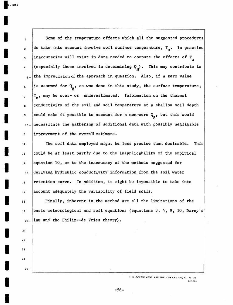
•• 1287


2

3

4

6

7

8

Some of the temperature effects which all the suggested procedures

do take into account involve soil surface temperature, T • In practice u

inaccuracies will exist in data needed to compute the effects of T u

(especially those involved in determining QN). This may contribute to

5 _ the imprecision of the approach in question. Also, if a zero value

is assumed for Q , as was done in this study, the surface temperature, g

T , may be over- or underestimated. Information on the thermal u

conductivity of the soil and soil temperature at a shallow soil depth

9 could make it possible to account for a non~ero Q , but this would g

10- necessitate the gathering of additional data with possibly negligible

11 improvement of the overall estimate.

12 The soil data employed might be less precise than desirable. This

13 could be at least partly due to the inapplicability of the empirical

14 equation 10, or to the inaccuracy of the methods suggested for

15- deriving hydraulic conductivity information from the soil water

16 retention curve. In addition, it might be impossible to take into

11 account adequately the variability of field soils.

1a Finally, inherent in the method are all the limitations of the

19 basic meteorological and soil equations (equations 3, 4, 9, 10, Darcy's

20_ law and the Philip--de Vries theory).

21

22

1 23

24

I I I

25-

-56-

U.S. GOVERNMENT PRINTING OFFICI::: 1959 0-511171

867 •IOU

•• 1287


2

3

4

6

7

8

9

With the surface-temperature equation 9 included in the

computation scheme, the procedure described in this paper might be

called quadri-comQinational, because it is an algorithm which combines

a soil equation of water flow and meteorological equations of heat

5- balance, vapor transfer and sensible heat transfer. Alternate forms of some of these equations

Jfould be employed and, possibly, other ways of including them in the

algorithm could be devised. The relative merits of such variants of

the proposed approach will have to be determined experimentally.

It follows from the above considerations that the technique

10- described in this paper is only approximate and that therefore it

11 should be used with appropriate care. It is possible to devise changes

12 in this technique which would considerably improve its precision.

13 However, these changes would imp~ir the ~ethod's relative simplicity

14 and its dependence on generally available data. The preliminary

15- experimental results cited above as well as theoretical considerations

16 seem to indicate that in spite of its limitations, the procedure for

17 evaluating evaporation presented in this paper can yield useful,

18 approximate estimates. It should be used primarily when simplicity

19 is needed and precision of estimates is not crucial.

20-

21

22

23

24

25-

-57-

U.S. GOVERNMENT PRINTING OFFICE: 1959 0-511171

867. 100

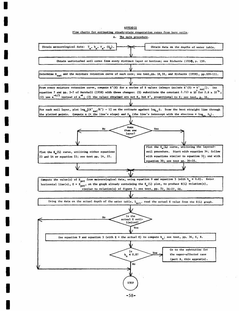
I


APPENDIX

Flow charts for est~ating steady-state evaporation rates from bare soils.

A. The main procedure.

Obtain meteorological data: Ta' ha' Va' (QN). Obtain data on the depths of water table.

Obtain undisturbed soil cores from every distinct layer or horizon; see Richards (195~, p. 159.

Determine Ksat and the moisture retention curve of each core; see text,pp. 16, 51, and Richards (1958), pp.109-lll.

From every moisture retention curve, compute K'(S) for a series of S values (always include K'(O) • K' !). Use 7

sat equation 7 and pp. 5-7 of Marshall (1958) with the•e changes: (1) substitute the constant 2.713 x lD for 2.8 x 10~;

(2) use n·4/ 3 instead of n-Q; (3) the values obtained are not K, but K', proportional to K; see text, • 16.

For each soil layer, plot lo~J(K'sat/K') • 1) on the ordinate against lo~0 S. Draw the best straight line through

the plotted points. Compute n (• the line's slope) and S (the line's intercept with the abscissa • lo

No

P~ot the E~(L) curve, utilizing either equations

23 and 14 or equation 25; see text pp. 14, 22.

Yes

Plot the E~(L) curve, utilizing the layered

soil procedure. Start with equation 34; follow

with to equation 3~; end with

Compute the value(s) of Epot from meteorological data, using equation 9 and equation 5 (with hu • 1.0). Enter

horizontal line(s), E = Epot' on the graph already containing the E~(L) plot, to produce E(L) relation(s),

similar to relation(s) of figure 7; see text, PP• 22 26-27 46.

Using the data on the actual depth of the water table, Lact' read the actual E value from the E(L) graph.

No

Use equation 9 and equation 5 (with E = the actual E) to compute hu; see text, pp. 36, 6, 8.

-58-

Go to the subroutine for

the vapor-affected case

(part B, this appendix).

I


B. The subroutine for the vapor-affected case.

Obtain data on T1

•

Using~ • 0.8, calculate Kliq (with equations 6 and 10) and Kvap·~ghDhv)/RT; see text, pp. 43, 7, 10.

Adjust the value of ~ •

For several arbitrary E values (not much different from the actual E, yielded by the aain

procedure), determine the corresponding Lu values (using equation 41); plot the relation

between Lu and E thus obtained; see text, pp. 42-43.

Plot the E.., (L) cu~ve, yielded. by the main procedure 6lith L = Lact - Lu •' ·where Lact • the actual

and L =a variablcl· Also plot the relation between L and E derived in the previous step. u u \

The intersection between these two curves determines the value of the actual E, adjusted for

vapor effects; see text, p. 44.

Redetermine T,_ ' * at smaller Lu;

see text, p. 44.

No

For several arbitrary E values (not much different from the actual E, yielded by the main

procedure) compute the values of~ and of the corresponding L', using equations 42 and 43; * u

plot the relation between Lu (= L~ + Lu) and E, based on this computation; see text, p. 44.

Plot the E=(L) curve, yielded by the Lact - Lu - Lu' where Lact = the

actual Land Lu = L~ + ~ "' a variable). Also plot the relation between Lu • L~ + L~ and E

derived in the previous step. The intersection between these two curves determines the value

• 45.

-59-

I •r,


i i

References

;Anat, Arbhabhirama, Duke, H. R.,and Corey, A. T., 1965, Steady upward · '

flow from water tables: Hydrology Paper No. 7, Coloradq State

Univ.,Fort Collins, Colo., 34 p.

; de Vries, D. A., 1958, Simultaneous transfer of heat and moisture in

porous media: Trans Amer. Geophys. Union, v. 39, p. 909-916.

: Edlefson, N. E., and Anderson, A. B. C., 1943, Thermodynamics of soil

moisture: Hilgardia, v. 15, p. 31-298.

Gardner, W. R., 1958, some steady-state solutions of the unsaturated

moisture flow equation with application to evaporation from a

water table: Soil Sci., v. 85, no. 4, p. 228-232.

--------~------1964, Water movement below the root zone, 8th Intern.

Congress of Soil Science, Bucharest, Rumania, v. II, p. 63-68.

--------------~and Fireman, M., 1958, Laboratory studies of

evaporation from soil columns in the presence of a water table:

Soil Sci., v. 85, no. 5, p. 244-249.

---------- and Hillel, D. I., 1962, The relation of external

evaporative conditions to the drying of soils: J. Geophys.

Research, v. 67, no. 11, p. 4319-4325.

. Gradshteyn, I. s., and Ryzhik, I. M., 1965, Table of Integrals, Series

and Products, Translated by A. Jeffrey, Academic Press, N.Y.,

1086 p.

Hanks, R. J., and Gardner, H. R., 1965, Influence of diffe~ent

diffusivity-water content relations on evaporation of water from

soils: Soil Sci ..... -~~.C: .. ~--~~:.::.· --~-:~-~-~ .. ! _'L~--~·-~'-·-~·()· 5, 1?~ .. 4_9~·498. ~ ... ' . • • '·I· .

-60-

1 t:.·~~


i ... ;

Harbeck, G. E., 1962, A practical field technique for measuring

reservoir evaporation utilizing mass-transfer theory: U.S. Geol.:

Survey Prof. Paper 272-E, p. El01-El05.

Hilqebrand, F. B., 1956, Introduction to Numerical Analysis, McGraw

Hill Book Co., N.Y., 511 P•

Jackson, Ray D., 1964, Water vapor diffusion in relatively dry soil.

II. Steady-state experim~nt: Soil Sci. Soc. Amer. Proc., v. 28,

no. 4, p. 467-470.

---------------- Reginato, R. J., and van Bavel, C. H. M., 1965,

Comparison of measured and calculated hydraulic conductivities of ·

unsaturated soils: Water Resources Res., v. 1, no. 3, p. 375-380.i

·List, R. J., 1951, Smithsonian Meteorological Tables, Misc.

Collections: v. 114, 527 p.

Marshall, T. J.~ 1958, The relation between permeability and size

distribution of pores: J. Soil Sci., v. 9, no. 1, p. 1-8.

Millington, R. J., and Quirk, J. P., 1961, Permeability of porous

solids: Trans. Faraday Soc., v. 57, p. 1200-1206.

Penman, H. L., 1940, Gas and vapour movements in the soil I. The

diffusion of vapours through porous solids: J. Agric. Sci.,

v. 30, p. 437-462.

Philip, J. R., 1957a, Evaporation, and moisture and heat fields in the

soil: J. Meteo~~ogy, ~· 14, p. 354-366.

_______________ 1957b, The physical principles of soil water movement

during the irrigation cycle: Trans. of Third Cong. on Irrigation

and Drainage, v. III, p. -~·.1_~?..:-.~~1~~· , .I 'I,\' . :.: ..

-61-

I·· !?~7

I I I I I I I • ..

I I I

I'

I I I I I I I I

r-- -·---··-----·---·--·----·--·-···-·---··----··· --,

I and de Vries, D. A., 1957, Moisture movement in porous i ,---------------I

material under temperature gradient: Trans. Amer. Geophys. Union,!

v. 38, p. 222-232.

Richards, L.A., (ed.), 1954, Diagnosis and improvement of saline and

alkali soils, Agricultural Handbook No. 60, USDA. I

. Rose, C. w., 1968, i

Water transport in soil with a daily temperature I I !

wave. I. Theory and experiment: Australian, Jou~ Soil Res.,

v. 6, p. 31-44.

:Rose, D. A., 1963a, Water movement in porous materials. Part 1.

u Isoth~rmal vap9f transfer: Brit. Jour. Appl. Phys., v. 14,

p. 256-262.

-----------1963b, Water movement in porous materials. Part 2. The

separation of the components of water movement: Brit. Jour. Appl.!

Phys., v. 14, p. 491-496.

·slatyer, R. 0., and Mcilroy, I.- C., 1961, Practical Microclimatology,

UNESCO (Prepared by CSIRO, Australia), 328 p.

Stallman, R. W., 1967, Flow in the zone of aeration: Adv. Hydrosci.,

v. 4, p. 151-195, ed. VenTe Chow, Academic Press, N.Y.

:van Bavel, C. H. M., 1966, Potential evaporation: The combination

concept and its experimental verification: Water Resources Res.,

~· 2, no. 3, p. 455-467.

van Hylckama, T. E. A., 1966, Evaporation from vegetated and fallow

soils: Water Resource.s Res., v. 2, no. 1, 99-103.

t • ,--i (,()\• I' ii!\,\'-!·:"., 1•1, :;. I II\ , ; t •

-62-

Documents

WATER RESOURCES DIVISION I ESTIMATING STEADY-STATE ... · The dependence of relative evaporation rates, 17 E/E po t' upon the potential evaporation rates, E po t' for 18 Chino clay-----29