VOL. 27, NO.1 WATER RESOURCES BULLETIN

AMERICAN WATER RESOURCES ASSOCIATION FEBRUAR.Y 1991

WATER QUAUTYTRENDSAT INFLOWS TO EVERGLADES NATIONAL PARKl

William W. Walker2

ABSTRACT: Wawr qII ality data rollected at infllJVfS w EVI:'rglllrles Nalion91 Park (ENP) are linalyzed fo!' trends using the seasonal Kendal! test (Hil"Jcli et cU., 1982; Hire<;h IlJld Slack, 1984). The peri­od of record ill 1977-1989 for innow. to Shark River Slough and 1983-1989 for innowll to Taylor Slough and ENPs Coastal Basin. The analy!;is considers 20 water quality components, including nutrients, field measurements, inorganic species. and opticnl prop­erties.

Significant (p<:O.10) increasing trends in total phosphorus con­centration are indicated at eight out of nine stations examined. When the data are adjusted to account for variations in antecedent rainfall and water surrace .. Ievation, increalling trends are indicat­ed at seven out of nine stations. Phosphorus trend magnitudes range from 4 percentJyear to 21 percent/year. Decreasing trends in the Thtal NIP ratio arc detected at seven out of nine stations. NIP trend magnitude.. range fmm -7 percent/year to -15 percentiyear. Trend. in water quality componenh other than nutrients are observed less frequently and a?'€ of Less importance from a water­quality-management perspective. The apparent nutrient tnmds are not expLained by v9.1'iatlnml In mat'Rh watCl' clcvntlMl, nnt~dent rainfall. flow, or season. (KEY TERMS: Evcrglad",,; &" .. ",,, .... \ K",,,dall le8t; w"Lcr quality; statistics; eutrophication; trend analysis; phosphon.l!l; nitrogen; nulrients; wetlands; Florida.)

INTRODUCTION

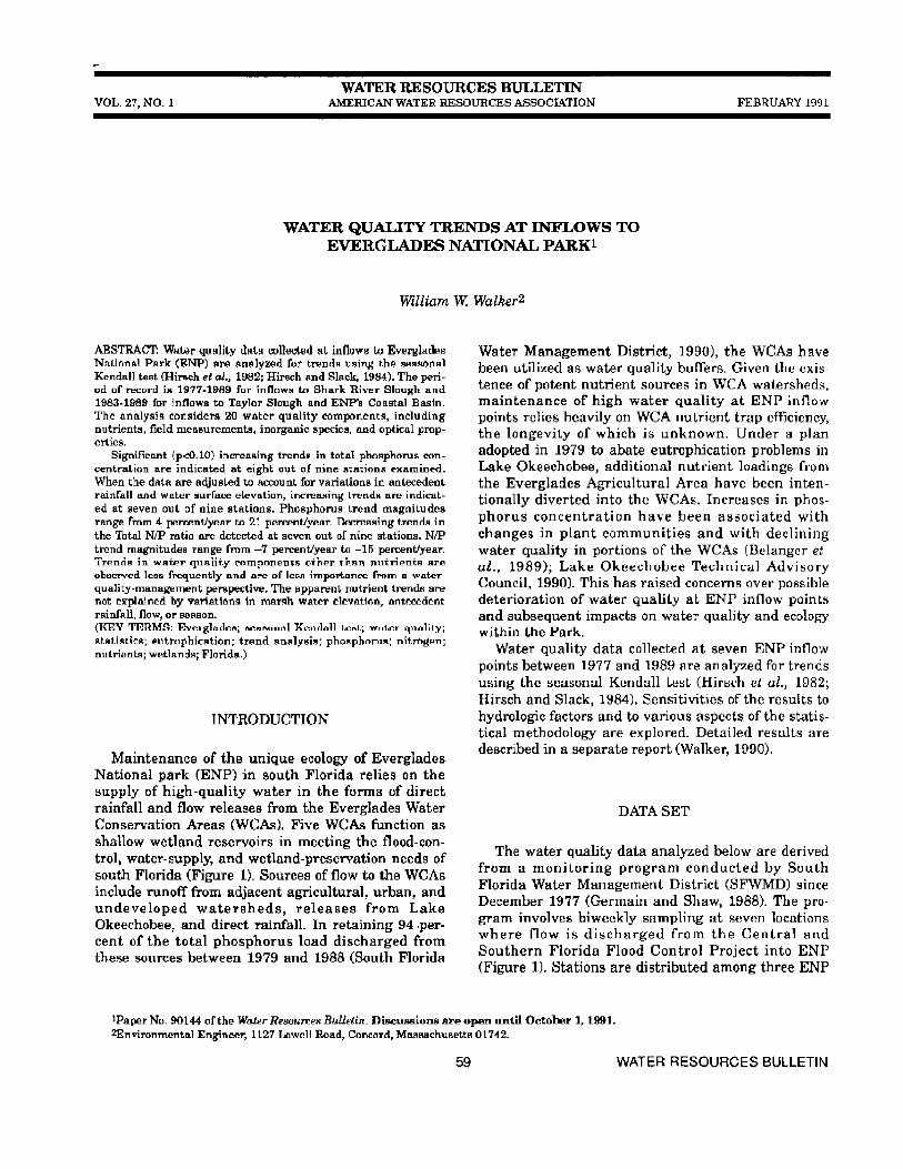
Maintenance of the unique ecology of Everglados National park (ENP) in south Florida relies Gn the supply of high-quality water in the forms of direct rainfall and flow releases from the Everglades Water Conservation Areas (WCAs). Five WCAs function as shallow wetland reservoirs in meeting the flood-con­tro], water-supply, and wetland-preservation needs of south Florida (Figure 1). Sources of flow to the WCAs include runoff from adjacent agricultural, urban, and undeveloped watersheds, releases from Lake Okeechobee, and direct rainfall. In retaining 94 per­cent of the total phosphorus load discharged from these sources between 1979 and 1988 (South Florida

Water Management District, 1990), the WCAs have been utilized as water quality buffers. Given the exis· tence of potent nutrient sources in WCA watersheds, maintenance of high water quality at ENP inflow points relics heavily on WCA nutrient trap efficiency, the longevity of which is unknown. Under a plan adopted in 1979 to abate eutrophication problems in Lake Okeechobee, additional nutrient loadings from the Everglades Agricultural Area have been inten­tionally diverted into the WCAs. Increases in phos­phorus concentration have been associated with changes in plant communities and with declining water quality in portions of the WCAs (Belanger et al., 1989); Lake Okeechobee Technical Advisory Council, 1990). This has raised concerns over possible deterioration of water quality at ENP inflow points and subsequent impacts on water quality and ecology within the Park.

Water quality data collected at seven ENP inflow points between 1977 and 1989 are analyzed for trends using the seasonal Kendall test (Hirsch et al., 1982; Hirsch and Slack, 1984). Scnsitivitics of the results to hydrologic factors and to various aspects of the statis­tical methodology are explored. Detailed results aTe described in a separate report (Walker, 1990).

DATASET

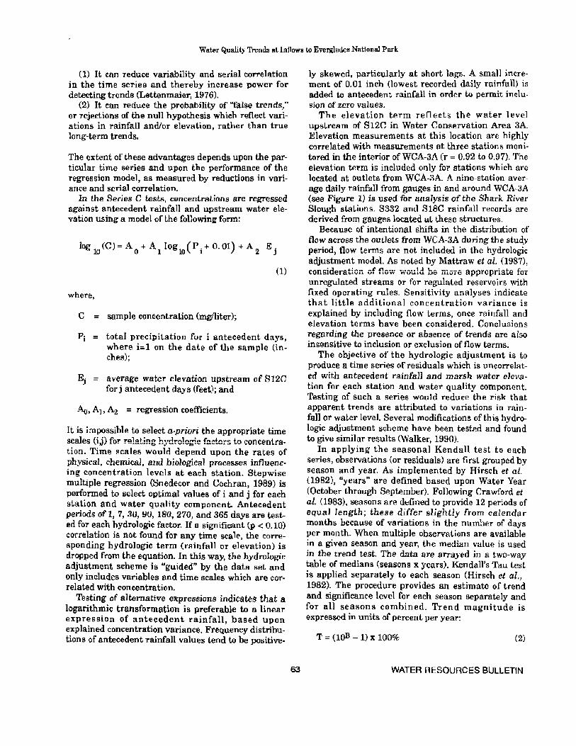
The water quality data analyzed below are derived from a monitoring program conducted by South Florida Water Management District (SFWMD) since December 1977 (Germain and Shaw, 1988). The pro­gram involves biweekly sampling at seven locations where flow is discharged from the Central and Southern Florida Flood Control Project into ENP (Figure 1). Stations are distributed among three ENP

lPaper No. 90144 of the Water ReWU7Ces BulieUn. DiscussioDfi are open until October I, 1991. 2Environmental Engineer, 1127 Lowell Road, Concord, Massachusetts 01742.

59 WATER RESOURCES BULLETIN

N

Everglades

Water

Conservation

Areas

, i.1 -I

Big Cypr ...

National

-. 1 L. _____ . _____ 1 ; Shark River

Everglades

National

Park

10 km

Slough

Florida Bay

/ I

• ENP Inflow Water Quality Station

~ Rainfall Gauge

--Canal or Levee

- - - - - ENP Boundary

Figure 1. Station Map.

WATER RESOURCES BULLETIN

Walker

60

watersheds: Shark River Slough (S12A, S12B, S12C, SI2D, and S333), Taylor Slough (S332), and Coastal (SI8C). The period of record is December 1977-September 1989 for Shark River Slough and October 1983-September 1989 for Taylor Slough and Coastal stations.

Two composite time series (SI2T and SI2.334) have been constructed by calculating flow-weigh ted­mean concentrations across structures in Shark River Slough on each sampling date. Station S 12T reflects total discharge Shark River Slough west of L67 (= S12A + S12B + S12C + SI2D). Station S12_334 reflects total discharge to Shark River Slough, includ­ing the Northeast portion. These composite series have been constructed to reflect total releases to Shark River Slough and to minimize effects of shifts in flow distribution across the individual outlet struc­tures during the monitoring period (SFWMD, 1990; Walker, 1990).

Detection of water quality trends is often compli­cated by hydrologic variations (Smith et al., 1982). Daily flow, water elevation, and rainfall measure­ments have been compiled for studying correlations between hydrology and water quality (SFWMD, 1988; USGS, 1989). A spatiallY'averaged rainfall time series for WCA-3A has been constructed by averaging data from nine gauges in and around the reservoir (Figure 1). Mean daily water surface elevation mea­sured by the U.S. Geological Survey upstream of S12C in WCA-3A provides an additional hydrologic variable for use in analyzing concentration data at inflows to Shark River Slough.

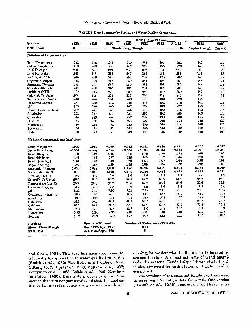
The analysis considers 20 water quality compo­nents, including nutrients, field measurements (dis­solved oxygen, temperature, pH, conductivity), inorganic species, and optical properties (color, turbid­ity). Table 1 summarizes the number of observations and median concentration for each station and water quality variable. Values reported below the detection limit have been set equal to the detection limit minus a small concentration increment (0.0001 mg/liter). In this way, such values can be distinguished from val­ues equal to the detection limit (Hirsch et al., 1982). Since the trend test is based upon ranks, the precise magnitude of the concentration increment does not influence computed significance levels. The percent­age of total phosphorus values reported below detec­tion limits ranges from 1 percent to 20 percent for the individual sampling stations.

STATISTICAL METHODS

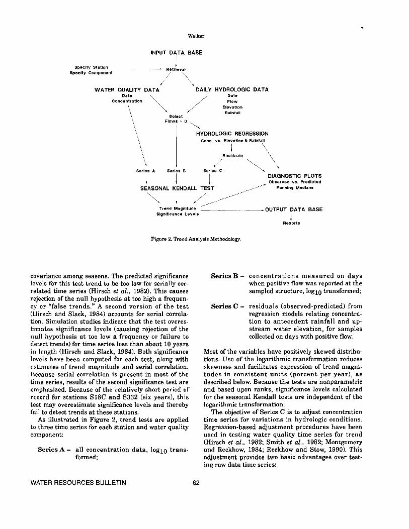
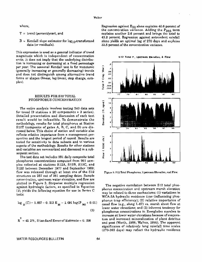
The trend analysis methodology (Figure 2) employs the seasonal Kendall test (Hirsch et al., 1982; Hirsch

Water Quality Trends at Inflows to EVI!rglades N ntional })ark

TABLE 1. Data Summary by Station and Water Quality Component.

ENP Inflow Station Station 81M 812B Si2C S]20 8l2l' saaa S12}IM S3a2 SlSC ENP Baain ~- - ---- ---- ---- ---- Shark River SlouCh ----- ------ ----- --- .... Taylor Sl~ ... eh Coalltal

N umb9r of ObservatlnllA

Total Phosphorus 241 246 255 249 281 196 281 143 118 Ortha Phosphorus 239 245 253 247 218 195 218 141 117 Thtal Nitrogen 244 249 257 250 282 194 282 146 122 ibial NIP Ratio 241 246 254 247 281 194 281 143 118 Total Kjeldahl N 244 249 258 251 282 196 282 146 122 Organ i~ Nitrogen 243 248 256 249 281 196 281 145 121 Ammonia Nitrogen 243 241 256 250 281 196 281 145 121 Nitrate+Nitrite N 244 248 256 251 281 194 281 146 122 Turbidity (NTU) 220 226 233 229 259 190 259 142 119 Col(>f (Pt-Co U nit.e) 209 214 222 217 246 179 246 U9 114 'llimpcralu.Te (neg'C) 240 244- 254 248 278 193 278 144 119 Dis.solved Oxygen 237 242 252 246 276 191 276 141 116 pH 233 238 24B 242 272 188 272 140 116 Conductivity (umhos) 237 241 251 245 275 190 275 142 118 Alkalinity 223 227 234 231 260 192 260 146 122 Chlorides 244 249 257 252 282 196 282 146 122 Calcium 81 15S 93 194 200 166 201 145 122 Magnesium SO 155 92 193 199 165 200 145 122 Potassium 50 125 51 141 145 134 145 132 l11 Sodium 50 125 51 143 147 136 148 145 121

Median C6noentratioDS (mlVliter)

'lbtal Phosphorus a.OIQ O.OIO (J.n 1O O.Q18 (J.Oll 0.014 O.()la [WO? V.{)/)7 Ortho Phosphorus <:0.004 <OJ)()4 <0.004 <0.004 <0.004 <;0.004 <0.004 <0.004 <0.004 Total Nitrogen 1.49 1.57 1.65 1.78 1.72 1.70 1.74 0.98 1.03

Total NIP Ratio 144 154 157 138 146 112 144 123 127

Total KjeldD.hl N 1.46 1.55 1.62 1.10 1.63 1.67 1.64 0.95 0.98

Organic Nil~g .. n 1.40 1.48 1.59 1.65 1.69 1.64 1.60 Q.'lB Q.&'l'

Ammonia Nitmgen 0.020 0.022 0.020 0.020 0.025 0.020 0.024 0.151 0.069 NitratuNitrite N 0.010 0.016 0.022 0.036 0.030 0.051 0.035 0.028 0.031

Turbidity (NTU) 0.9 0.9 1.0 1.0 1.0 1.1 1.1 2.5 1.9

Color (Pt,..Co Unit.l1) 28.0 38.0 51.2 58.3 48.2 63.7 54.2 26.2 26.4

1ernperature(deg-C) 25.7 25.8 25.2 25.6 25.7 26.1 25.6 25.5 25.5 Dissolved Oxygen .t.7 4.0 3.8 3.9 3.9 3.6 3.8 ,"-I 5.4

pH 7.21 7.11 7.10 7.24 7.18 7.19 7.1M 1.19 7.35

Conductivity (umhos) :iDH 361 485 617 512 65B 547 495 ~na

""" Alkalinity 120 133 161 191 167 201 177 1m! 203 Chlorides 22.6 30.6 50.2 68.9 50.5 82.0 58.5 36.5 53.7

Calcium 40.1 46.8 53.5 62.5 57.7 63.5 60.1 72.8 75.3

Magmlsiurn 3.0 4.1 8.3 12.8 9.0 14.9 11.1 5.1 6.9

PotassiuID 0.93 1.34 2.36 2.86 2.21:1 3.24 2.85 1.12 2.78

Sodium 13.2 21.3 35.9 44.S 35.4 52.6 42.3 22.7 33.3

ShttioJUl Ptlriod of Record N"mher ofWatu YearWVariable Shark Riy_ Slough Dec. 1977&pt. Ul89 S332, Sli!C Oct. 1983-Sept. 1989

and Slack, 1984). This test hal; been recommended frequently for application to water quality time series (Smith et al., 1982; Van Belle and Hughes, 1984; Gilbert, 1987; Ripel et al., 1988; Mattraw et aL 1987; Berryman et 01., 1988; Loftis et 01., 1989; Reckhow and Stow, 1990). Desirable properties of the test include that it is nonparametric and that it is applica­ble to time series containing values which are

61

U-12 6

missing, below detection limits, andior influenced by seasonal factors. A robust estimate of trend magni­tude, the seasonal Kendall slope (Hirsch et at., 1982), is also computed for each station and water quality component.

Two versions of the seasonal Kendall tes.t are used in screening ENP inflow data for trends. One version (Hirsch et ai., 1982) assumes that there is no

WATER RESOURCES BULLETIN

Walker

INPUT DATA BASE

j ---- Retrieval Specify Station

Specify Component

/ ~ WATER QUALITY DATA DAIL Y HYDROLOGIC OAT A

Dale Concentration ~ /

Oat ..

Flow Elevation Rainfall

Series A

j

Select Flows' 0

Series B

j

~ HYDROLOGIC REGRESSION

Cone. va. Elevation 8. Rainfall

,.,,(,""!"'" '''\ j DIAGNOSTIC PLOTS

Observed va. Predicted

SEASONAL KENDALL TEST ~~~

~ J ~~~~ Running Medians

Trend Magnitude ---------OUTPUT DATA BASE Significance Levels j

Reports

Figure 2, Trend Analysis Methodology,

covariance among seasons, The predicted significance levels for this test trend to be too low for serially cor­related time series (Hirsch et al., 1982). This causes rejection of the null hypothesis at too high a frequen­cy or "false trends," A second version of the test (Hirsch and Slack, 1984) accounts for serial correla­tion, Simulation studies indicate that the test overes­timates significance levels (causing rejection of the null hypothesis at too Iowa frequency or failure to detect trends) for time series less than about 10 years in length (Hirsch and Slack, 1984), Both significance levels have been computed for each test, along with estimates of trend magnitude and serial correlation, Because serial correlation is present in most of the time series, results of the second significance test are emphasized. Because of the relatively short period of record for stations S18C and S332 (six years), this test may overestimate significance levels and thereby fail to detect trends at these stations.

As illustrated in Figure 2, trend tests are applied to three time series for each station and water quality component:

Series A - all concentration data, 10glO trans­formed;

WATER RESOURCES BULLETIN 62

Series B - concentrations measured on days when positive flow was reported at the sampled structure, 10glO transformed;

Series C - residuals (observed-predicted) from regression models relating concentra­tion to antecedent rainfall and up­stream water elevation, for samples collected on days with positive flow,

Most of the variables have positively skewed distribu­tions, Use of the logarithmic transformation reduces skewness and facilitates expression of trend magni­tudes in consistent units (percent per year), as described below, Because the tests are non parametric and based upon ranks, significance levels calculated for the seasonal Kendall tests are independent of the logarithmic transformation.

The objective of Series C is to adjust concentration time series for variations in hydrologic conditions, Regression-based adjustment procedures have been used in testing water quality time series for trend (Hirsch et ai., 1982; Smith et al" 1982; Montgomery and Re ckh ow, 1984; Reckhow and Stow, 1990). This adjustment provides two basic advantages over test­ing raw data time series:

Water Quality Trend!! at In!lows to Evergladce National Park

(1) It cnn reduce variability and serial correlation in the time series and thereby increase power for detecting trends (Lettenmaier, 1976).

(2) It can reduce the probability of "'false trends, n

or rejections of the null hypothesis which reflect vari­ations in rainfall andior elevation, rather than true long-term trends.

The extent of these advantages depends upon the par­ticular time series and upon the performance of the regression model, as measured by reductions in vari­ance and serial correlation.

In the Series C tests, concentrations are regressed against antecedent rainfall and upstream water ele­vation using a model of the following form:

(1)

where,

C = sample concentration (mgiliter);

Pi = totnl precipitation for i antecedent days. where i=l on the date of the sample (in­ches);

Ej = average water elevation upstream of S12C for j antecedent days (feet); and

Ao. AI, ~ = regression coefficients.

It is impossible to select a-priori the appropriate time sca.Jes (ij) for relating hydrologic factors to concentra­tion. Time scales would depend upon the rates of physical. chemical. and biological pmcesses influenc­ing concentration levels at each station. Stepwise multiple regression (Snedecor and Cochran, 1989) is performed to select optimal values of i and j for each station and water quality component. Antecedent periods of 1, 7, 30, 90, 180, 270, and 365 days are test­ed fol' each hydrologic factor. If a significant (p < 0.10) correlation is not found for any time scale, the corre­sponding hydrologic term (rainfall or elevation) is dropped from the equation. In this way, the hydrologic adjustment scheme is "guided" by the data set and only includes variables and time scales which are cor­related with concentration.

Testing of alternative expressions indicates that a logarithmic transformation is llreferable to a linear expression of antecedent r~infal1, based up-~n explained concentration variance. Frequency distribu­tions of antecedent rainfall values tend to be positive-

63

ly skewed, particularly at short lags. A small incre­ment of 0.01 inch (lowest recorded daily rainfall) is added to antecedent rainfall in order to permit inclu­sion of zero values.

The elevation term reflects the water level upstream of S12C in Water Conservation Area 3A. Elevation measurements at this location are highly correlated with measurements at three stations moni­tored in the interior of WCA-3A (r = 0.92 to 0.97). The elevation term is included only for stations which are located at outlets from WCA-3A. A nine-station aver­age daily rainfall from gauges in and around WCA-3A (see Figure 1) is used for ana1ysis of the Shark River Slough stations. S332 and S18C rainfall record:> are derived from gauges located ut these stmctures.

Because of intentional shifts in the distribution of flow across the outlets from WCA-3A during the study period, flow terms arc not included in the hydrologic adjustment model. As noted by Mattraw et al. (1987), consideration of flow would be more appropria.te for unregulated streams or for regulated reservoirs with fixed operating rules. Sensitivity analyses indicate that little additional concentration variance is explained by including flow terms, once rainfall and elevation terms have been considered. Conclusions regarding the presence or absence of trends are also insensitive to inclusion or exclusion of flow terms.

The objective of the hydrologic adjustment is to produce a time series of residuals which is uncorrelat­ed with antecedent rainfall and marsh water eleva­tion for each station and water quality component. Testing of such a series would reduce the risk that apparent trends are attributed to variations in rain­fall or water level. Several modifications of this hydro­logic adjustment scheme have been tested and found to give similar results (Walker, 1990).

In applying the seasonal Kendall test to each series, observations (or residuals) are first grouped by season and year. As implemented by Hirsch et al. (1982), "year:»" are defined based upon Water Year (October through September). Following Crawford et ai. (1983), seasons are defined to provide 12 periods of equal length; these differ slightly from calendar months because of variations in the number of days per month_ When multiple observations are available in a given season and year, the median value is used in the trend test. The data are arrayed in a two-way table of medians (seasons x years). Kendall's Tau test is applied separately to each season (Hirsch et al., 1982). The procedure provides an estimate of trend and significance level for each season separately and for all seasons combined. Trend magnitude is expressed in units of percent per year: -

T = (loB - 1) x 100% (2)

WATER RESOURCES BULLETIN

Walker

where,

T = trend (percent/year), and

B ;;; Kendall slope estimator for loglO-transformed data (or residuals).

This expression is used as a general indicator of trend magnitude which is independent of concentration units. It does not imply that the underlying distribu­tion is increasing or decreasing at a fixed percentage per year. The seasonal Kendall test is for monotonic (generally increasing or generally decreasing) trends and does not distinguish among alternative trend forms or shapes (linear, log-linear, step change, com­plex).

RESULTS FOR S12 TOTAL PHOSPHORUS CONCENTRATION

The entire analysis involves testing 540 data sets for trend (9 stations x 20 components x 3 series). Detailed presentation and discussion of each test result would be infeasible. To demonstrate the methodology, results for total phosphorus at Station S12T (composite of gates A, B, C, and D) are dis­cussed below. This choice of station and variable also reflects relative importance from a management per­spective and the longest period of record. Results are tested for sensitivity to data subsets and to various aspects of the methodology. Results for other stations and variables are summarized and discussed in a sub­sequent section.

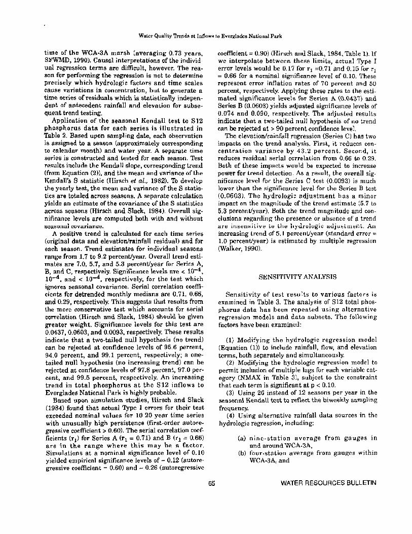
The test data set includes 281 daily composite total phosphorus concentrations computed from 991 sam­ples collected at stations S12A, S12B, S12C, and 812D between December 1977 and September 1989; flow was released through at least one of the S 12 structures on 257 out of 281 sampling dates. Sample concentration, upstream water elevation, and flow are plotted in Figure 3. Stepwise multiple regression against hydrologic factors, as specified in Equation (1), yields the following equation for use in Series C tests:

log 10 (C) = 1.857 - O. 213 E ill - 1 001Iog(P 365 + 0.01)

(3)

2 R = 43. 2%, Standard Error of Estimate = 0.236

WATER RESOURCES BULLETIN 64

Regression against Eao alone explains 40.6 percent of the concentration variance. Adding the P365 term explains another 2.6 percent and brings the total to 43.2 percent. Regression against antecedent rainfall alone yields an optimal lag of 270 days and explains 33.5 percent of the concentration variance.

! :=

QI E

!1.

! 0 I-

"C > QI r::

--r:: 0 ;;:;

'" > 41 iij

J!! u o o o ,....

~ o i!

.2

.1

.06

.04

.02

.01

.006

.004

.002

11

10

9

8

7

6

5

S 12 Total P, Upstream Elevation, & Flow

77 79 81 83 85 87 89

Figure 3.812 Total Phosphorus, Upstream Elevation, and Flow.

The negative correlation between 812 total phos­phorus concentration and upstream marsh elevation may be related to three mechanisms: (1) variations in WCA-3A hydraulic residence time (influencing phos­phorus trap efficiency); (2) relative importance of canal flow (e.g., along L-67) vs. marsh sheet flow at lower water elevations; and (3) inherent tendency for phosphorus concentrations in Everglades marshes to increase at lower water elevations because of evapora­tion and increased mineralization of plant detritus and peat (Worth, 1988; Walker, 1990). The apparent significance of relatively long rainfall time scales (270-365 days) may reflect the hydraulic residence

Wat.cr Quality Trends at Inflow. to Everglades National Park

time of the WCA-3A marsh (averaging 0.73 years, SFWMD, 1990), Causal interpretations of the individ­ual regression terms are difficult, however. The rea­son for performing the regression is not to determine precisely which hydrologic factors and time scales cauSe variations in concentration, but to generate a time series of residuals which is statistically indepen­dent of antecedent rainfall and elevation for subse­quent trend testing,

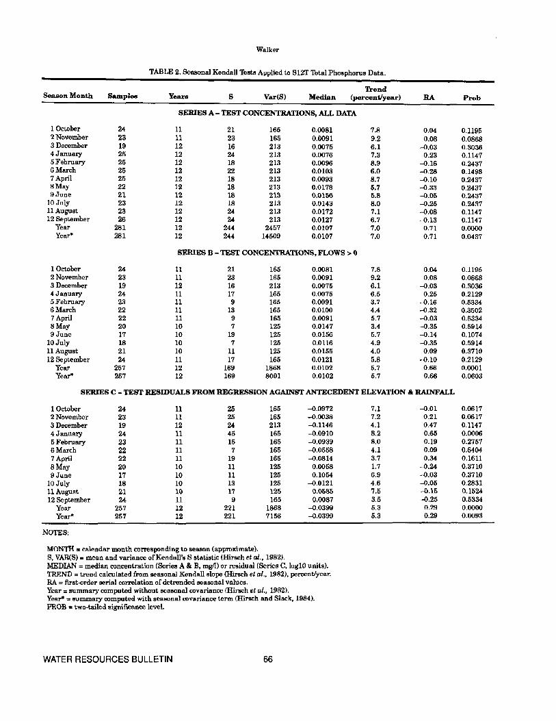
Application of the seasonal Kendall test to 812 phosphorus data for each series is illustrated in Table 2. Based upon sampling date, each observation is assigned to a season (approximately corresponding to calendar month) and water year. A separate time series is constructed and tested for each season. Test results include the Kendall slope, corresponding trend (from Equation (2)), and the mean and variance of the Kendall's S statistic (Hirsch et ai., 1982). To develop the yearly test, the mean and variance of the S statis­tics are totaled across seasons. A separate calculation yields an estimate ofthe covariance of the S statistics across seasons (Hirsch and Slack, 1984). Overall sig­nificance levels are computed both with and without seasonal covariance.

A positive trend is calculated for each time series (original data and elevation/rainfall residual) and for each season. Trend estimates for individual seasons range from 1.7 to 9.2 percenUyear. Overall trend esti­mates are 7.0, 5.7, and 5.3 percent/year for Series A, B, and C, rel'lpectlvely. S;gnificance levels aTe <; 10-4. 10-4, and < 10-4, respectively, for the test which ignores seasonal covariance. Serial correlation coeffi­cients for detrended monthly medians are 0.71, 0.66, and 0.29, respectively. 'I'his suggests that results from the more conservative test which accounts for serial corTelation (Hirsch and Slack, 1984) should be given greater weight. Significance levels for this test are 0.0437,0.0603, and 0,0093, respectively. These results indicate that a two-tailed null hypothesis (no trend) can be rejected at confidence levels of 95.6 percent, 94.0 percent, and 99.1 percent, respectively; a one­tailed null hypothesis (no increasing trend) can be rejected at confidence levels of 97.8 percent, 97.0 per­cent, and 99,5 percent, respectively. An increasing trend in total phosphorus at the 812 inflows to Everglades National Park is high Iy probable.

Based upon simulation studies, Hirsch and Slack (1984) found that actual Type 1 errors for their test exceeded nominal values for 10-20 year time series with unusually high persistence (first-order autore­gressive coefficient> 0.60). The serial correlation coef­ficients (r1) for Series A (rl = 0.71) and B (r1 :::: 0.66) are i.n the range where this may be 8 factor, Simulations at a nominal significance level of 0.10 yielded empirical significance levels of - 0.12 (autore­gressive coefficient = 0.60) and - 0.26 (autoregressive

65

coefficient = 0.90) {Hirsch and Slack, 1984, Table n If we interpolate between these limits, actual Type I error levels would be 0.17 for r1 =0.71 and 0.15 for r1 = 0.66 for a nominal significance level of 0.10. These represent error inflation rates of 70 percent and 50 percent, respectively. Applying these rates to the esti­mated significance levels fm- Series A (0.0431) and Series B (0.0603) yields adjus~d significance levels of 0.074 and 0.090, respectively. The adjusted results indicate that a two-tailed null hypothesis of no trend can be rejected at > 90 percent confidence level.

The elevation/rainfall regression (Senes C) has two impacts on tbe trend analysis. First, it reduces con­centration variance by 43.2 percent. Second, it reduces rBsidual serial correlation from 0.66 to 0.29. Both of these impacts would be expected to increase power for trend detection. As a rf!!Hl It, the overall sig­nificance level for the Series C test (0.0093) is much lower than the signilicance level for the Series B test (0.0603). The hydrologic adjustment has a minor impact on the magnitude of the trend Bstimate (5.7 to 5.3 percent/year). Both the trend magnitude and con­clusions regarding the presence or absence of a trend are insensitive to the hydrologic adjustment. An increasing trend of 5.1 percenUyear (standard error = 1.0 percent/year) is estimated by multiple regression (Walker, 1990).

SENSITIVITY ANALYSIS

Sensitivity of test results to various factors is examined in Table 3. The analysis of S12 total phos­phorus data has been repeated using alternative regression models and data subsets. The fonowing factors have been examined:

(1) Modifying the hydrologic regression model (Equation (1) to include rainfall, flow, and elevation terms, both separately and simultaneously.

(2) Modifying the hydrologic regression model to permit inclusion of multiple lags for each variable cat­egory (NMAX in Table 3), subject to the constraint that each term is significant at p < 0.10.

(3) Using 26 ins~ad of 12 seasons per year in the seasonal Kendall test to reflect the biweekly sampling frequency.

(4) Using alternative rainfall data sources in the hydrologic regression, including:

(a) nine-station average from gauges in and around WCA-3A,

(b) four-station average from gauges within WCA-3A, and

WATER RESOURCES BULLETIN

Walker

TABLE 2. Seasonal Kendall Tests Applied to SI2T Total Phosphorus Data.

'hend Season Month Sampl_ Years S Var(S) Median (percent/year) RA Prob

SERIES A - TEST CONCENTRATIONS, ALL DATA

1 October 24 11 21 166 0.0081 7.8 0.04 0.1195 2 Novemher 23 11 23 165 0.0091 9.2 0.08 0.0868 3 December 19 12 16 213 0.0075 6.1 ~.03 0.3036 4 January 25 12 24 213 0.0076 7.3 0.23 0.1147 5 February 25 12 18 213 0.0096 8.9 ~.16 0.2437 6 March 25 12 22 213 0.0103 6.0 ~.28 0.1498 7 April 25 12 18 213 0.0093 8.7 ~.10 0.2437 8 May 22 12 18 213 0.0178 5.7 -0.33 0.2437 9 June 21 12 18 213 0.0156 5.8 -0.05 0.2437

10 July 23 12 18 213 0.0143 8.0 -0.25 0.2437 11 August 23 12 24 213 0.Q172 7.1 ~.08 0.1147 12 September 26 12 24 213 0.0127 6.7 ~.13 0.1147

Year 281 12 244 2467 0.0107 7.0 0.71 0.0000 Year* 281 12 244 14509 0.0107 7.0 0.71 0.0437

SERIES B - TEST CONCENTRATIONS, FLOWS>.,

1 October 24 11 21 165 0.0081 7.8 0.04 0.1195 2 November 23 11 23 165 0.0091 9.2 0.08 0.0868 3 December 19 12 16 213 0.0075 6.1 ~.03 0.3036 4 January 24 11 17 165 0.0075 6.5 0.26 0.2129 5 February 23 11 9 165 0.0091 3.7 ~.16 0.5334 6 March 22 11 13 165 0.0100 4.4 -0.32 0.3502 7 April 22 11 9 165 0.0091 5.7 ~.03 0.5334 8 May 20 10 7 125 0.0147 3.4 ~.35 0.5914 9 June 17 10 19 125 0.0156 5.7 ~.14 0.1074

10 July 18 10 7 125 0.0116 4.9 ~.35 0.5914 11 August 21 10 11 125 0.0155 4.0 0.09 0.3710 12 September 24 11 17 165 0.0121 5.8 -0.10 0.2129

Year 257 12 169 1868 0.0102 5.7 0.66 0.0001 Year* 257 12 169 8001 0.0102 5.7 0.66 0.0603

SERIES C - TEST RESIDUALS FROM REGRESSION AGAINST ANTECEDENT ELEVATION 01: RAINFALL

1 October 24 11 25 165 ~.0972 7.1 ~.01 0.0617 2 November 23 11 25 165 ~.0038 7.2 0.21 0.0617 3 December 19 12 24 213 ~.1146 4.1 0.47 0.1147 4 January 24 11 45 165 ~.0910 8.2 0.65 0.0006 5 February 23 11 15 165 ~.0939 8.0 0.19 0.2757 6 March 22 11 7 165 ~.0558 4.1 0.09 0.6404 7 April 22 11 19 165 ~.0814 3.7 0.34 0.1611 8 May 20 10 11 125 0.0058 1.7 ~.24 0.3710 9 June 17 10 11 125 0.1054 6.9 -0.03 0.3710

10 July 18 10 13 125 -0.0121 4.6 ~.05 0.2831 11 August 21 10 17 125 0.0585 7.5 -0.15 0.1524 12 September 24 11 9 165 0.0087 3.5 -0.25 0.5334

Year 257 12 221 1868 -0.0399 5.3 0.29 0.0000 Year* 257 12 221 7156 -0.0399 5.3 0.29 0.0093

NOTES:

MONTH '" calendar month corresponding to season (approximate). S, VAR(S) = mean and variance of Kendall's S statistic (Hirsch et aI., 1982). MEDIAN '" median concentration (SeriCll A & B, mgIl) or residual (Series C, loglO units). TREND = trend calculated from !leasonal Kendall slope (Hirsch et al., 1982), percentJycar. RA = fIrSto()rder serial correlation of detrended seasonal values. Year = summary computed without f!eMonal covariance (Hirsch et aI., 1982). Year* = 8u=ary computed with seasonal covariance term (Hirsch and Slack, 1984). FROB = two-tailed significance level.

WATER RESOURCES BULLETIN 66

Water Quality Trendl! at Inflows to Everglades National Park

(c) vAlues from a single station closest to the S12's (southwest ofS12A, Figure 1).

This series of regressions also considers extended rainfall lags beyond one year (1, 7, 30, 90, 180, 270, 365,545,730, and 910 days) and includes any regres­sion term significant at p < 0.10.

(5) Excluding data from January I-September 15, 1985 (duration of the pho5phoros spike in Figure 3, associated with low WCA·3A water elevations and open 812 gates).

(6) Considering wet season (May~October) vs. dry season (Novemool'-April) data separately.

(7) Considering low-elevation « 9.4 feet) vs. high­elevation (> 9.4 feet) observations separately; eleva­tion cutpoint selected to divide data set roughly in half.

(8) Excluding periods of extreme low elevation c< 8 feet), associated with phosphorus spikes in Figure 3.

(9) Considering low-flow (<: 500 cfs) VB. high-flow (> 500 cfs) data separately; flow cutpoint selected to divide data set roughly in half.

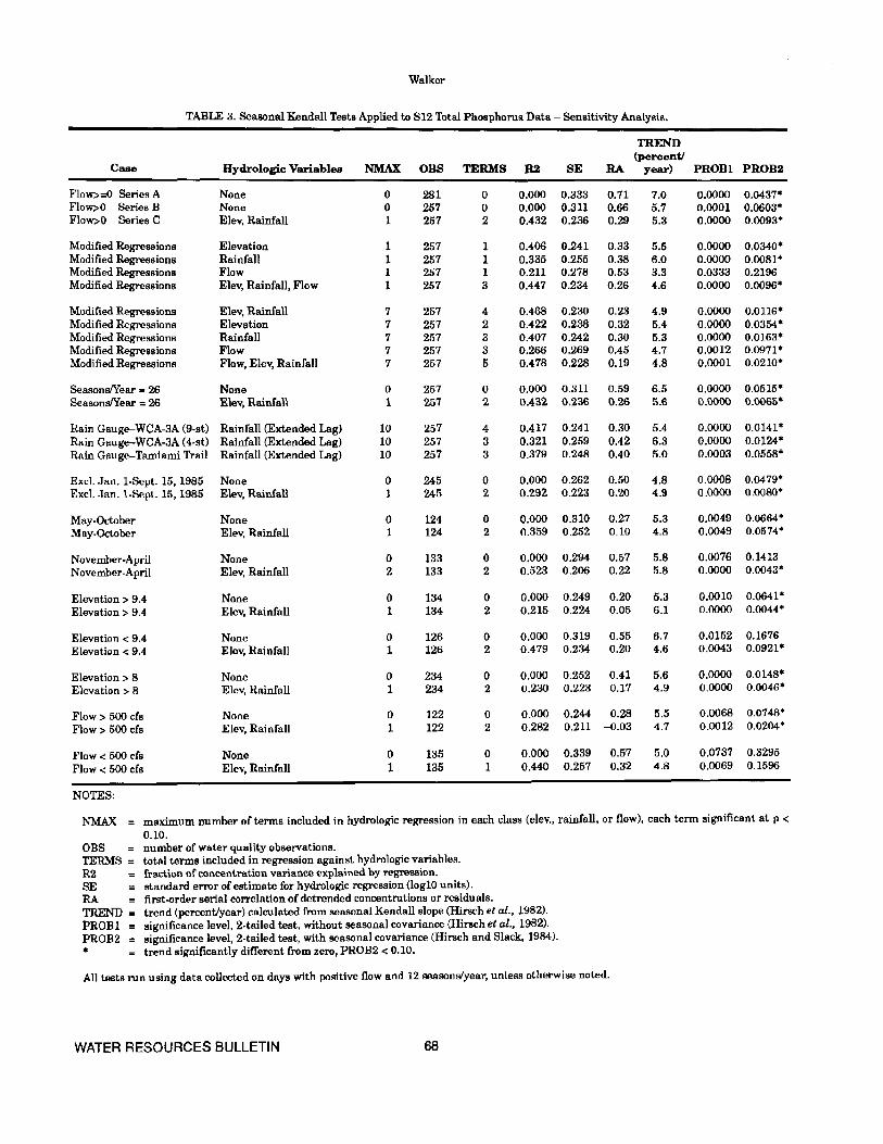
Thst results are generally insensitive to these factors. Estimated trend magnitudes range from 3.3 to 7.0 percent/year. Significance levels for the more conser­vative test accounting for serial correlation are below 0.10 in 28 out of 33 tests summarized in Table 3.

Results are insensitive to modifications in the hydrologic Tegression model, number of seasons per year, rainfall data source, and wet-season vs. dry-sea­son subsets. When flow alone is used in the hydrologic regression equation, the significance level increases to 0.2196. Flow explains only 21.1 percent of the vari­ance of the concentration variance, however, as com­pared with 33.5 percent for antecedent rainfall and 40.6 percent for elevation. Adjustment based upon flow is complicated by increases in 8333 flows and deCTcaos,cs 1n 812 flows which occurred in and after 1984 as a result of changes in water management strategies. The presence of a significant increasing trend when data from January I-September 15, 1985, are excluded indicates that the trend is not explained by the phosphorus spike evident in Figure 3,

When the sensitivity analysis in Table 3 is repeat­ed using the combined discharge to Shark River Slough (Station 812_334), significance levels are below 0.06 in every case except for the low-flow and low-elevation data sets. The relative weakness of trends in low-flow or low-ell!vation sampll!s partially reflects the fact that concentrations are more variable under these conditioll!i. For example, the log-scale standard deviation of the low-flow and high -flow data sets for 812T are 0,339 and 0.244, respectively. Higher variabiljty makes it more difficult to identify trends. Another important factor contributing to

67

higher significance levels is that the number of obser· vations is cut in half when the data set is split; this reduces the power of the test. Despite differences in significance levels, estimates of trend magnitude are similar for the low-flow vs. high-flow data sets and for the low-elevation vs. high·elevation data sets. The fact that trends are more distinct under high-flow conditions is important because such conditions are primarily responsible for phosphorus transport into the Park. Analysis of 812 daily now data for water years 1978-1989 indicates that flow rates exceeding 500 cfs accoWlted for 87 percent of the total discharge volume ruld 49 percent of tbe tota1 days.

RESULTS FOR OTHER STATIONS AND COMPONENTS

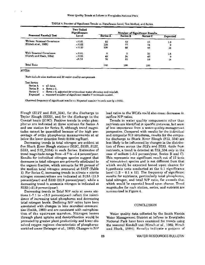
The seasonal Kendall test has been applied to data for each station and water quality component. Detailed results are reported in Walker (1990), Table 4 summarizes the number of significant test results as a functiun uf probability level « 0,01, < 0.05, <: 0.10), test method (with VB. without seasonal covari­ance), and test series (A, B, and C). Application of the more conservative test which accounts for serial cor­relation reduces the number of significant results, particularly at the 0.01 test level. The number of sig­nificant -results in each cate~()1"Y faT exceeds that which would be expected based upon chance if no trends existed, For example, 52 Series B results out of 180 tests had significance levels less than 0.10. If no trends existed, the expected number of significant results would be 18 (= 0.10 x 180).

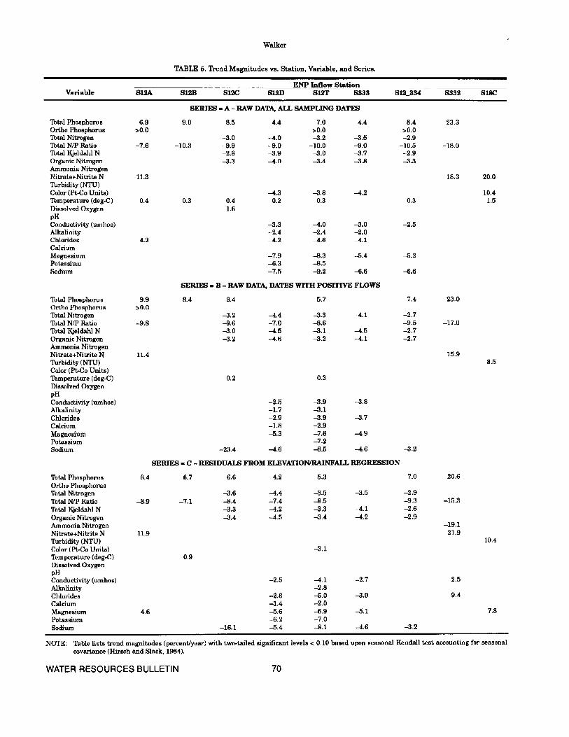
Table 5 lists estimated trend magnitudes for each station, variable, and series for all tests with two­tailed significance levels less than 0.10 using the more conservative lest (Hirsch and Slack, 1984). Increasing trends in total phosphorus are indicated in at least one test series (A, B, or C) at eight out of nine stations (excluding S18C). With adjustments for antecedent elevation and rainfall (Series C), increas­ing trends are indicated at seven out of nine stations (excluding 8333 and SI8C). An increasing phosphorus trend (9.1 percent/year) is also likely at SIBC, based upon the estimated significance level for Series B and C (p = 0.1048) and the tendency for the test to overestimate significance levels in time series less than 10 years in length (Hirsch and Slack, 1984). Trend magnitudes in residuals range from 4.2 per­cent/year for S 12D to 20.6 percent/year for 8332. Conclusions regarding the presence or absence of trend, as well as trend magnitudes, are insensitive to hydrologic adjustment of the time series (Series B vs. Series C) fOT the combined di'behal'ge'b ro Shark Rivet

WATER RESOURCES BULLETIN

Walker

TABLE 3. Seasonal Kendall Tests Applied to S12 '!btal Phosphorus Data ~ Sensitivity Analysis.

TREND (percentJ

Case Hydrologic Variables NMAX ODS TERMS R2 SE RA year) PROBl PROB2

Flow>::O Series A None 0 281 0 0.000 0.333 0.71 7.0 0.0000 0.0437* Flow>O Series B None 0 257 0 0.000 0.311 0.66 5.7 0.0001 0.0603" Flow> 0 Series C Elev. Rainfall 1 257 2 0.432 0.236 0.29 5.3 0.0000 0.0093"

Modified Regressions Elevation 1 257 1 0.406 0.241 0.33 5.5 0.0000 0.0340· Modified Regressions Rainfall 1 257 1 0.335 0.255 0.38 6.0 0.0000 0.0081* Modified Regressions Flow 1 257 1 0.211 0.278 0.53 3.3 0.0333 0.2196 Modified Regressions Elev, Rainfall, Flow 1 257 3 0.447 0.234 0.26 4.6 0.0000 0.0096·

Modified Regressions Elev. Rainfall 7 257 4 0.468 0.230 0.23 4.9 0.0000 0.0116· Modified Regressions Elevation 7 257 2 0.422 0.238 0.32 5.4 0.0000 0.0354· Modified Regressions Rainfall 7 257 3 0.407 0.242 0.30 5.3 0.0000 0.0163* Modified Regressions Flow 7 257 3 0.266 0.269 0.45 4.7 0.0012 0.0971· Modified Regresl!ions Flow, Elev, Rainfall 7 257 5 0.478 0.228 0.19 4.8 0.0001 0.0210·

SeaaonslYear = 26 None 0 257 0 0.000 0.311 0.59 6.5 0.0000 0.0515· SeasonslYear = 26 Elev, Rainfall 1 257 2 0.432 0.236 0.26 5.6 0.0000 0.0065"

Rain Gauge-WCA-3A (9-st) Rainfall (Extended Lag) 10 257 4 0.417 0.241 0.30 5.4 0.0000 0.0141* Rain Gauge-WCA-3A (4-8t) Rainfall (Extended Lag) 10 257 3 0.321 0.259 0.42 6.3 0.0000 0.0124· Rain Gauge-Tamiami Trail Rainfall (Extended Lag) 10 257 3 0.379 0.248 0.40 5.0 0.0003 0.0558*

Exe!. Jan. I-Sept. 15, 1985 None 0 245 0 0.000 0.262 0.50 4.8 0.0008 0.0479" Rxcl .• Jan. I-Sept. 15, 1985 Elev, Rainfall 1 245 2 0.292 0.223 0.20 4.9 0.0000 0.0080*

May-Oct~ber None 0 124 0 0.000 0.310 0.27 5.3 0.0049 0.0664· May-October Elev, Rainfall 1 124 2 0.359 0.252 0.10 4.8 0.0049 0.0574*

November-April None 0 133 0 0.000 0.294 0.57 5.8 0.0076 0.1413 November-April Elev, Rainfall 2 133 2 0.523 0.206 0.22 5.8 0.0000 0.0043*

Elevation> 9.4 None 0 134 0 0.000 0.249 0.20 5.3 0.0010 0.0641 • Elevation> 9.4 Elev, Rainfall 1 134 2 0.215 0.224 0.05 6.1 0.0000 0.0044·

Elevation < 9.4 None 0 126 0 0.000 0.319 0.55 6.7 0.0152 0.1676

Elevation < 9.4 Elev, Rainfall 1 126 2 0.479 0.234 0.20 4.6 0.0043 0.0921*

Elevation> 8 None 0 234 0 0.000 0.252 0.41 5.6 0.0000 0.0148*

Elevation> 8 Elcv, Rainfall 1 234 2 0.230 0.223 0.17 4.9 0.0000 0.0046"

Flow> 500 efa None 0 122 0 0.000 0.244 0.28 5.5 0.0066 0.0748*

Flow> 500 cfs Elev, Rainfall 1 122 2 0.282 0.211 -0.03 4.7 0.0012 0.0204*

Flow < 500 cfs None 0 135 0 0.000 0.339 0.57 5.0 0.0737 0.3295

Flow < 500 cfs Elev, Rainfall 1 135 1 0.440 0.257 0.32 4.8 0.0069 0.1596

NOTES:

NMAX maximum number of terms included in hydrologic regression in each class (elev., rainfall, or flow), cach term significant at p < 0.10.

OBS number of water quality observations. TERMS total terms included in regression against hydrologic variables. R2 fraction of concentration variance explained by regression. SE standard error of estimate for hydrologic regression (log10 units). RA first-order serial correlation of detrended concentrations or residuals. TREND = trend (percent/year) calculated from seasonal Kendall slope (Hirsch et aI., 1982). PROBI significance level. 2-tailed test, without seasonal covariance (Hirsch et aI., 1982). PROB2 significance level, 2-tailed test, with seasonal covariance (Hirsch and Slack, 1984).

* trend significantly different from zero, PROB2 < 0.10.

All tests run using data collected on days with positive flow and 12 seasons/year, unless other-wise noted.

WATER RESOURCES BULLETIN 68

Water Quality Trends at Inflows to Everglades National Park

TABLE 4. Nllmbe,r of Significant Trend.. vs. Significance Level, Test Method, Ilnd Series.

Witbout &I\sonal Covariance (Hirsch et ol., 1982)

With Seasonal Covariance (HiNch and Slack, 1984)

'Ibtal Tests

NOTES:

Two-Tailed Sipificanee

L.eve!

<0.01 <0.05 <O.lD

<0.01 <0.05 <0.10

ThBte include nine Btationa Bnd 2Q wBter quality components

Test Series: all data. flows> O.

S9rieeA

92 109 120

6

49 70

lAO

Nwuber of SiJillficllnt Results

53 51 77 74 88 88

5 16 34 43 52 58

100 180

L8 9

18

1.8 9

18

Serle<! A Series B Series C Expect.ed

flows» 0, a.;ljuatad for ant(l<ledent water elevation and rainfall. expected number Df significant results if no trends existed.

Observed frequency of significant results » Expected number in each case (p < 0.05).

Slough (812T and S12_334), for the discharge to Taylor Slough (8332), and for the discharge to the Coastal basin (S18C). Positive tTends in ortho phos­phorus are indieated at three stations for Series A and one station for Series B, although trend magni­tudes eannot be quantified because of the high per­centage of ol'tho phosphorus measurements at or below the 10wer detection 1imit (0.004 mgIJiter).

Decreasing trends in total nitTogen are evident at five Shark River Slough stations (S12C, SI2D, Sl2T, 5333, and SI2_8334) in eacll Series. Estimates of trend magnitude range from -2.7 to -4.4 percent/year. Resuits for individuai nitrogen species suggest that decreases in total nitrogen are primarily attributed to the organic fraction, which accounts for 92 percent of the median total nitrogen measured at S12T (Table 1). For Series C, increasing trends in nitrate + nitrite nitrogen concentrations are indicated at S12A (11.9 percent/year) and 8332 (21.9 percent/year), while a decreasing trend is ammonia nitrogen is indicated at 8332 (-21.9 percent/year).

Decreasing trends in Total NIP ratio at seven sta­tions (-7.1 to -15.3 percent/year) reflect the coinci­dence of increasing total phosphot'Us and decreasing total nitrogen levels. Declining NIP ratios have been associated with changes in lake microbial communi-6es (Smith, 1983) and are consistent with eutTophica­tion of the upstream marshes. Nitrogen losses through plant uptake and denitrification \~ou]d be promoted by greater plant productivity and lower dis­solved oxygen regimes eharacteristie of phosphorus­enriched ~ones (Belanger et al., 1989). Changes in NIP

69

load ratios to the WCNs could also cause deereases in outflow NIP ratios.

Trends in water quality eomponents other than nutrients are identified in specific instances, but seem of less importance from a water-quality-management perspective. Compared with results for the individual and composite 812 structures, results for the compos­ite discharge to Shark River Slough (S 12_334) are less likely to be influenced by changes in the distribu­tion of flows acrOSS the 812's and 8333. Aside from nutrients, a trend IS detecl.ed at 812_334 on1y in the case of sodium (-3.2 percent/year, Series B and C). This represents one significant result out of 12 test::; of nonnutrient species and is not different from that which would be expected based llllon chance for hypothesis tests conducted at the 0.1 significance level (1.2 = 0.1 x 12). The frequency of significant results for nutrients, particularly total phosphorus, total nitrogen, and total NIP ratio, far exceeds that which would be expected based upon chance. Trend magnitudes for each station, series, and nutrient are summarized in Figure 4.

CONCLUSION

Water quality data coUected b::; the South F1()1'1da 'lIster ~1anag2ment District at inf1o\vs to Everglades National Park have been examined for trends using the seasona1 Kendall test (Hirsch et al., 1982; Hirsch and Slack, 1984). Rp.sults indicate a pattern of

WATER RESOURCES BULLETIN

Walker

TABLE 5. Trend Magnitudes vs. Station, Variable, and Series.

El'!PJnflow S~tion Variable Sl2A Sl2B Sl2C S12I) Sl2T 8333 S12_334 8332 SlBC

SERIES. A - RAW DATA, ALL SAMPUNG DATES

'Ibtal Phosphorus 6.9 9.0 8.5 4.4 7.0 4.4 8.4 23.3 Ortho Phosphorus >0.0 >0.0 >0.0 'Ibtal Nitrogen -3.0 -4.0 -3.2 -3.5 -2.9 'Ibtal NIP Ratio -7.6 -10.3 -9.9 -9.0 -10.0 -9.0 -10.5 -18.0 Total lijeldahl N -2.8 -3.9 -3.0 -3.7 -2.9 Organic Nitrogen -3.3 -4.0 -3.4 -3.8 -3.3 Ammonia Nitrogen Nitrate+Nitrite N 11.3 18.3 20.0 Turbidity (NTU) Color (Pt-Co Units) -4.3 -3.8 -4.2 10.4 Temperature (deg-C) 0.4 0.3 0.4 0.2 0.3 0.3 1.5 Dissolved Oxygen 1.6 pH Conductivity (umhos) -3.3 -4.0 -3.0 -2.5 Alkalinity -2.4 -2.4 -2.0 Chlorides 4.2 -4.2 -4.6 ---4.1 Calcium Magnesium -7.9 -8.3 -5.4 ~".2 Potassium -6.3 -8.5 Sodium -7.5 -9.2 -6.6 -6.6

SERIES. B - RAW DATA, DATES WITH POSITIVE FLOWS

Total Phosphorus 9.9 8.4 8.4 5.7 7.4 23.0 Ortho Phosphorus >0.0 'Ibtal Nitrogen -3.2 -4.4 -3.3 -4.1 -2.7 Total NIP Ratio -9.8 -9.6 -7.0 -8.6 -9.5 -17.0 Total Kjeldahl N -3.0 -4.5 -3.1 -4.5 -2.7 Organic Nitrogen -3.2 -4.6 -3.2 -4.1 -2.7 Ammonia Nitrogen Nitrate+Nitrite N 11.4 15.9 Turbidity (NTU) 8.5 Color (Pt-Co Units) Temperature (deg-C) 0.2 0.3 Dissolved Oxygen pH Conductivity (umhos) -2.5 -3.9 -3.8 Alkalinity -1.7 -3.1 Chlorides -2.9 -3.9 -3.7 Calcium -loll -2.9 Magnesium -5.3 -7.6 -4.9 Potassium -7.2 Sodium -23.4 -4.6 -8.5 -4.6 -3.2

SERIES. C - RESIDUAUl FROM ELEVATIONIRAINFALL REGRESSION

Total Phosphorus 6.4 6.7 6.6 4.2 5.3 7.0 20.6 Mho Phosphorus Total Nitrogen -,'3.6 -4.4 -3.5 -3.5 -2.9 'Ibtal NIP Ratio -8.9 -7.1 -8.4 -7.4 -8.5 -9.3 -15.3 Total Kjeldahl N --3.3 -4.2 --3.3 -4.1 -2.6 Organic Nitrogen --3.4 -4.5 -3.4 -4.2 -2.9 Ammonia Nitrogen -19.1 Nitrate+Nitrite N 11.9 21.9 Turbidity (NTU) 10.4 Color (Pt-Co Units) --3.1 Temperature (deg-C) 0.9 Dissolved Oxygen pH Conductivity (umhos) -2.5 -4.1 -2.7 2.5 Alkalinity -2.8 Chlorides -2.8 -5.0 --3.9 9.4 Calcium -1.4 -2.0 Magnesium 4.6 -5.6 -6.9 -5.1 7.8 Potassium -6.2 -7.0 Sodium -16.1 -5.4 -8.1 -4.6 --3.2

NOTE: Table lists trend magnitudes (percent/year) with two-tailed significant levels < 0.10 based upon seasonal Kendall test accounting for seasonal covariance (Hirseh and Slack, 1984).

WATER RESOURCES BULLETIN 70

Water Quality Trend! at InflDws to Everglades NatiDnal Park

Nutrient Trend Magnitudes

VS. Station and Data Series

Taylor ENP Basin: --- -- Shark River Slough ~ - ,_ Slough Coastal

"Q C (I) .. ....

24 r---------------------------------------------------nn7Tr----------, Total Phosphorus

20

16

....

e L... Total Nitrogen

r-4 f-

f-

•• f::~ II ••

.:: {r

.: 1-:---"~.,,'t~':",.,.'=.-·~:-.·,..,r;,-"'----,w_r* . ....,,:J."";;~-~-.--rU-,-.:."..·\~j!I-----r~-,-·*:"·~j"..~,-*..-r.t.,.,*Ig::i:~':~ ~ ....... ..

r-

-8 I-

S1ZA SHe S12D S1'2T

-4

-8

-12

-16

Total N/P Ratio -20

Sl2& S'2C 812D S12T

s18e

n:-\~

S1BC

S18C

C3 Series A , All Data

[?3J Series B '" ,. Flows> 0

Series C - Elevation/Rainfall Residual

Trends Significant at p < .10 ell:) or p ( .05 ('1'*)

Figure 4. Nutrient Trend Magnitudes VB. Station and Data Series.

71 WATER RESOURCES BULLETIN

Walker

increasing phosphorus concentrations and decreasing NIP radios at ENP inflow points. Conclusions regard­ing the presence or absence of nutrient trends are insensitive to adjustment of the time series to account for variations in hydrologic factors (rainfall, water elevation, or flow). Trends detected for the 1977 to 1989 period cannot be extrapolated into the past or into the future. The analysis does not distinguish among alternative trend shapes (linear, exponential, step change at a specific date) or identify specific causes. Increasing phosphorus concentrations and decreasing NIP ratios are symptoms of eutrophica­tion, a process which must be avoided if the unique water quality and ecology of ENP marshes are to be preserved.

ACKNOWLEDGMENTS

This analysis was supported by the U.S. Department of Justice, Environment and Natural Resources Division. Daniel Sheidt, Robert Johnson, and David Sikkema of the Everglades National Park Research Laboratory assisted in supply data and reviewing the manuscript. Comments by Dennis Helsel, James Slack, and Aaron Higer of the U.S. Geological Survey, J ames Loftis of Colorado State University, Robert Gcrzoff of Environ Corporation, and AWRA reviewers are also gratefully acknowledged.

LITERATURE CITED

Belanger, T. V., D. J. Scheidt, and J. R. Platko, 1989. Effects of Nutrient Enrichment on the Florida Everglades. Lake and Reservoir Management 5(1);101-112.

Berryman, D., B. Bobee, D. Cluis, and J. Haemmerli, 1988. Nonparametric Tests for Trend Detection in Water Quality Time Series. Water Resources Bulletin 24(3);545-556.

Crawford, C. G., J. R. Slack, and R. M. Hirsch, 1983. Nonpara­metric Tests for Trends in Water-Quality Data Using the Statistical Analysis System. U.S. Geological Survey, Open-File Report 83.550.

Germain, G. J. and J. E. Shaw, 1988. Surface Water Quality Network. South Florida Water Management District, Technical Publication 88-3.

Gilbert, R. 0., 1987. Statistical Methods for Environmental Pollution Monitoring. Van Nostrand.

Hipel, K. W., A. I. McLeod, and R. R. Weiler, 1988. Data Analysis of Water Quality Time Series in Lake Erie. Water Resources Bulletin 24(3):533-544.

Hirsch, R. M. and J. R. Slack, 1984. A Nonparametric Trend Test for Seasonal Data with Serial Dependence. Water Resources Re!learch 20(6):727-732.

Hirsch, R. M., J. R. Slack, and R. A. Smith, 1982. Techniques of Trend Analysis for Monthly Water Quality Data. Water Resources Research 18(1):107-121.

Lake Okeechobee Technical Advisory Council (LOTAC II), 1990. Final Report to State of Florida.

Lettenmaier, D. P., 1976. Detection of Trends in Water Quality Data from Records with Dependent Observations. Water Resources Research 12(5):1037-1046.

Loftis, J. C., R. C. Ward, R. D. Phillips, and C. Taylor, 1989. An Evaluation of Trend Detection Techniques for Use in Water

WATER RESOURCES BULLETIN 72

Quality Monitoring Programs. U.S. Environmental Protection Agency, Office of Acid Deposition Environmental Monitoring and Quality Assurance, Washington, D.C., EPN600/3-89/037.

Mattraw, H. C., D. J. Scheidt, and A. C. Federico, 1987. Analysis of Trends in Water-Quality Data for Water Conservation Area 3A, The Everglades, Florida. U.S. Geological Survey, Water Resources Investigations Report 87-4142.

Montgomery, R. H. and K. H. Reckhow, 1984. Techniques for Detecting Trends in Lake Water Quality. Water Rcsources Bulletin 20( 1):43-52.

Reckhow, K. H. and C. Stow, 1990. Monitoring Design and Data Analysis for Trend Detection. Lake and Reservoir Management 6(1):49-60.

Smith, R. A., R. M. Hirsch, and J. R. Slack, 1982. A Study of Trends in 'Ibtal Phosphorus Measurements at Stations in the NASQAN Network. U.S. Geological Survey, Water Supply Paper 2190.

Smith, V., 1983. Low Nitrogen to Phosphorus Ratios Favor Dominance by Blue-Green Algae in Lake Phytoplankton. Science 221:669-671.

Snedecor, G. W. and W. G. Cochran, 1989. Statistical Methods, 8th Edition. The Iowa State University Press, Ames, Iowa.

South Florida Water Management District, 1988. Access to the South Florida Water Management District Hydrologic Data Base. Data Management Division, Version 3.t.

South Florida Water Management District, 1990. Everglades SWIM Plan (draft).

U.S. Geological Survey, 1989. Water Resources Data for Florida. Miami, Florida, Office.

Van Belle, G. and J. P. Hughes, 1984. Nonparametric Tests for Trend in Water Quality. Water Resources Research 20(1):127-136.

Walker, W. W., 1990. Water Quality Trends at Inflows to Everglades National Park. Prepared for U.S. Department of Justice, Environment and Natural Resources Division, Washington, D.C.

Worth, D. F., 1988. Environmental Response of WCA-2A to Reduction in Regulation Schedule and Marsh Drawdown. Technical Publication No. 88-2, South Florida Water Management District.