Embed Size (px)
Citation preview

WATER DISTRIBUTION SYSTEM DESIGN AND REHABILITATION UNDER CLIMATE CHANGE MITIGATION
SCENARIOS
by
Ehsan Roshani
A thesis submitted to the Department of Civil Engineering
In conformity with the requirements for
the degree of Doctor of Philosophy
Queen’s University
Kingston, Ontario, Canada
(April 2013)
Copyright © Ehsan Roshani, 2013

ii
To My Father

iii
Abstract
The water industry is a heavy consumer of electricity to pump water. Electricity generated with
fossil fuel sources produce greenhouse gas (GHG) emissions that contribute to climate change.
Carbon taxation and economic discounting in project planning are promising policies to reduce
GHG emissions. The aim of this research is to develop novel single- and multi-objective
optimization frameworks that incorporate a new gene-coding scheme and pipe ageing models
(pipe roughness growth model, a pipe leakage model, and a pipe break model) to examine the
impacts of a carbon tax and low discount rates on energy use, GHG emissions, and
design/operation/rehabilitation decisions in water systems. Chapter 3 presents a new algorithm
that optimizes the operation of pumps and reservoirs in water transmission systems. The
algorithm was applied to the KamalSaleh transmission system near Arak, Iran. The results
suggest that a carbon tax combined with a low discount rate produces small reductions in energy
use and GHG emissions linked to pumping given the high static head of the KamalSaleh system.
Chapter 4 presents a new algorithm that optimizes the design and expansion of water distribution
networks. The algorithm was applied to the real-world Fairfield water network in Amherstview,
Ontario, Canada. The results suggest that a carbon tax combined with a low discount rate does not
significantly decrease energy use and GHG emissions because the Fairfield system had adequate
installed hydraulic capacity. Chapters 5 and 6 present a new algorithm that optimizes the optimal
rehabilitation type and timing of water mains in water distribution networks. In Chapter 5, the
algorithm is applied to the Fairfield network to examine the impact of asset management
strategies (quantity and infrastructure adjacency discounts) on system costs. The results suggest
that applying discounts decreased capital and operational costs and favored pipe lining over pipe
replacement and duplication. In Chapter 6, the water main rehabilitation optimization algorithm is
applied to the Fairfield network to examine the impact of a carbon tax and low discount rates on

iv
energy use and GHG emissions. The results suggest that adopting a low discount rate and levying
a carbon tax had a small impact in reducing energy use and GHG emissions and a significant
impact in reducing leakage and pipe breaks in the Fairfield system. Further, a low discount rate
and a carbon tax encouraged early investment in water main rehabilitation to reduce continuing
leakage, pipe repair, energy, and GHG costs.

v
Co-Authorship
This thesis represents mainly original work by the author; however, significant contributions were
made by co-authors who collaborated in interpreting the results and preparing journal and
conference papers, some of which have been used in modified forms as chapters in this thesis.
Chapters 3, 4, 5, and 6 were written as independent journal manuscripts that have been published
in, or submitted to, peer-reviewed journals. Dr. Yves Filion, provided intellectual supervision and
editorial comments for all chapters and is a co-author of all the manuscripts. Stephanie P.
MacLeod, M.A.Sc., is also a co-author of Chapter 4. Stephanie prepared the case study data and
helped in the preparation and writing of the manuscript.

vi
Acknowledgements
I would like to express my sincere gratitude to my supervisor, Dr. Yves Filion, for his
encouragement, patience and guidance throughout the course of the project and also for his
incredible generosity with his time and knowledge. His constructive suggestions and comments
on my work have been invaluable, and have enabled me to develop this research to its fullest
potential. I enjoyed the privilege of doing this research with him. I have benefited immensely
from his support and I consider myself lucky to have worked with Dr. Filion. I am deeply
indebted for all his efforts.
I also would like to gratefully acknowledge Stephanie P. MacLeod, M.A.Sc., who played an
essential role in the success of this thesis. Stephanie contributed immensely in preparing Chapter
4. My warmest regards goes to David Thompson, P.Eng. and Jason Sands at Loyalist Township
for providing invaluable information and professional contribution to the development of this
thesis. This research was financially supported by Queen’s University and the Natural Sciences
and Engineering Research Council (NSERC).
I am sincerely thankful to Dr. Ian Moore at Queen’s University, Dr. Ahmad Malekpour and Dr.
Bryan Karney at University of Toronto, Dr. Steven Buckberger at University of Cincinnati, Dr.
Zoran Kapelan at University of Exeter, and Dr. Kevin Lansey at University of Arizona for
valuable discussion and encouragement and for sharing their practical experiences with me.
I would like to thank Ms. Maxine Wilson and Mr. Bill Boulton at the Department of Civil
Engineering at Queen’s University for their incredible support. In addition I would like to thank
my friends, A. Kanani, L. Herstein, Dr. R. Valipour, A. Oldford, and H. Swartz for their input,
support, and friendship.

vii
I would also like to acknowledge the contribution made by my parents Omran and Fozieh
Roshani and my sisters Kosar and Elham. Thank you for your support and endless
encouragements. Finally, I must express my deepest gratitude to my love, Rezvan, whose
unconditional love and support through the last 10 years gave me the strength and hope to live.

viii
Table of Contents
Abstract .....................................................................................................................................iii Co-Authorship ............................................................................................................................v Acknowledgements ....................................................................................................................vi List of Figures..........................................................................................................................xiii List of Tables ............................................................................................................................xv Chapter 1 Introduction.................................................................................................................1
1.1 Research Background ........................................................................................................1 1.2 Research Objectives ..........................................................................................................7 1.3 Thesis Organization...........................................................................................................9 1.4 Publication Related to the Thesis .....................................................................................10
1.4.1 Journal Papers...........................................................................................................10 1.4.2 Papers in Conference Proceedings.............................................................................11
1.5 References.......................................................................................................................12 Chapter 2 Problem Definition and Literature Review.................................................................19
2.1 Water distribution system design, expansion and rehabilitation as an optimization problem.
.............................................................................................................................................19 2.1.1 WDS Design.............................................................................................................21 2.1.2 WDS Expansion .......................................................................................................21 2.1.3 WDS Operation ........................................................................................................26 2.1.4 WDS Rehabilitation ..................................................................................................29
2.2 Incorporating economic measures to mitigate GHG emission in the problem formulation.34 2.3 GA-Based Single- and Multi-Objective Optimization ......................................................38
2.3.1 Introduction to the GA ..............................................................................................38 2.3.2 GA operators ............................................................................................................40 2.3.3 Single-Objective GA, Elitist GA ...............................................................................42 2.3.4 Multi-Objective GA, NSGA-II ..................................................................................42 2.3.5 Penalty Functions......................................................................................................44
2.4 OptiNET..........................................................................................................................44 2.4.1 Asset Management and Model Validation .................................................................45
2.5 Research Contributions....................................................................................................46

ix
2.5.1 Publication 1: “Impact of Uncertain Discount Rates and Carbon Pricing on the Optimal
Design and Operation of the KamalSaleh Water Transmission System” .............................48 2.5.2 Publication 2: “Evaluating the Impact of Climate Change Mitigation Strategies on the
Optimal Design and Expansion of the Fairfield, Ontario Water Network: A Canadian Case
Study” ...............................................................................................................................49 2.5.3 Publication 3: “Event-Based Approach to Optimize the Timing of Water Main
Rehabilitation While Considering Asset Management Strategies” ......................................50 2.5.4 Publication 4: “Water Distribution System Rehabilitation under Climate Change
Mitigation Scenarios in Canada”........................................................................................51 2.6 References.......................................................................................................................52
Chapter 3 Impact of Carbon-Mitigating Strategies on Energy Use and Greenhouse Gas Emissions
in the KamalSaleh Water Transmission System: A Real Case Study ..........................................65 3.1 Abstract...........................................................................................................................65 3.2 Introduction.....................................................................................................................66
3.2.1 Economic Instruments to Mitigate GHG Emissions...................................................66 3.2.2 Previous Research in the Optimization of Sustainable Water Distribution Networks ..68
3.3 KamalSaleh Water Transmission: Single-objective and Multi-objective Optimization ......72 3.3.1 Multi-Objective Optimization Formulation ...............................................................74 3.3.2 Single-Objective Optimization Formulation ..............................................................77 3.3.3 Optimization Constraints...........................................................................................78 3.3.4 Reservoir and Pump Operation Constraints ...............................................................79
3.4 Gene Coding Scheme for Pump Scheduling .....................................................................81 3.4.1 Elitist Genetic Algorithm ..........................................................................................82 3.4.2 Non-Dominated Sorting Genetic Algorithm (NSGA-II).............................................82
3.5 Case Study: KamalSaleh Water Transmission Pipeline ....................................................83 3.6 Single-Objective Optimization Results.............................................................................86
3.6.1 Impact of Discount Rate on Optimal Design, Costs, Electricity Use, and GHG
Emissions ..........................................................................................................................87 3.6.2 Impact of a Carbon Tax on Optimal Design, Costs, Electricity Use, and GHG
Emissions ..........................................................................................................................88 3.6.3 Combined Impact of a Carbon Tax and Discount Rates on the Optimal Design, Costs,
Electricity Use, and GHG Emissions..................................................................................88 3.7 Multi-Objective Optimization Results..............................................................................89

x
3.8 Discussions and Interpretation of Results .........................................................................93 3.9 Summary and Conclusions...............................................................................................94 3.10 Acknowledgements .......................................................................................................95 3.11 References .....................................................................................................................95
Chapter 4 Evaluating the Impact of Climate Change Mitigation Strategies on the Optimal Design
and Expansion of the Fairfield, Ontario Water Network: A Canadian Case Study ....................100 4.1 Abstract.........................................................................................................................100 4.2 Introduction...................................................................................................................100 4.3 Research in Planning, Design, and Optimization of Water Distribution Networks for
Environmental Sustainability...............................................................................................102 4.3.1 NRTEE Carbon Pricing...........................................................................................104 4.3.2 Social Discount Rates Suggested by the Treasury Board of Canada.........................104
4.4 Problem Formulation .....................................................................................................106 4.5 Case Study: Optimization of the Fairfield Water Distribution Network ..........................109
4.5.1 Demand Conditions ................................................................................................111 4.5.2 Capital Costs...........................................................................................................113 4.5.3 Operational Cost .....................................................................................................115 4.5.4 GHG Emissions ......................................................................................................116 4.5.5 GHG Cost...............................................................................................................117
4.6 Results ..........................................................................................................................118 4.7 Discussion .....................................................................................................................122 4.8 Summary and Conclusions.............................................................................................124 4.9 Acknowledgments .........................................................................................................125 4.10 References ...................................................................................................................125
Chapter 5 Event-Based Approach to Optimize the Timing of Water Main Rehabilitation with
Asset Management Strategies ..................................................................................................131 5.1 Abstract.........................................................................................................................131 5.2 Introduction...................................................................................................................132 5.3 Problem Definition ........................................................................................................136 5.4 Event-Based Rehabilitation: A New Approach to Gene Coding......................................138 5.5 Asset Management Strategies ........................................................................................140 5.6 Model Implementation...................................................................................................142 5.7 Fairfield Water Distribution Network.............................................................................143

xi
5.7.1 Pipe Leakage Model ...............................................................................................146 5.7.2 Break Model ...........................................................................................................147 5.7.3 Pipe Roughness Growth Model ...............................................................................148
5.8 Asset Management Scenarios and Results ......................................................................149 5.8.1 Pareto-Fronts of Scenarios 1 Through 4 ..................................................................149 5.8.2 Impact of the Budget Constraint and Discounts on Capital and Operational Costs ...152 5.8.3 Impact of Discounts on the Geographic Location of Rehabilitated Pipe ...................153 5.8.4 Impact of Budget Constraint and Discounts on the Occurrence of Rehabilitation Events
........................................................................................................................................155 5.8.5 Impact of Budget Constraint on the Annual Costs ...................................................157
5.9 Sensitivity Analysis .......................................................................................................159 5.10 Summary and Conclusions...........................................................................................161 5.11 Acknowledgements .....................................................................................................162 5.12 References ...................................................................................................................162
Chapter 6 Water Distribution System Rehabilitation under Climate Change Mitigation Scenarios
in Canada................................................................................................................................167 6.1 Abstract.........................................................................................................................167 6.2 Introduction...................................................................................................................167
6.2.1 Greenhouse Gas Emissions, Carbon Tax, and Economic Discounting in Canada .....168 6.3 Review of Previous Research in Network Rehabilitation and Sustainable Network Design
...........................................................................................................................................170 6.4 Problem Definition ........................................................................................................173
6.4.1 Leak Forecasting Model..........................................................................................174 6.4.2 Break Forecasting Model ........................................................................................175 6.4.3 Pipe Roughness Growth Forecasting Model ............................................................176 6.4.4 Model Implementation ............................................................................................176
6.5 Fairfield Water Distribution Network.............................................................................178 6.6 Results and Discussions.................................................................................................181
6.6.1 Effect of Discount Rate and Carbon Tax on the Location of Pareto Fronts...............182 6.6.2 Effect of Discount Rate and Carbon Tax on Energy Use and GHGs ........................184 6.6.3 Effect of Discount Rate and Carbon Tax on Water Loss and Break Repair Cost ......189 6.6.4 Effect of Discount Rate and Carbon Tax on Rehabilitation Decision Type and Timing
........................................................................................................................................189
xii
6.6.5 Differences in Leakage Costs, Pipe Break Repair Costs, and Energy Costs across
Minimum Capital Cost Solutions and Minimum Operational Cost Solutions ....................191 6.7 Sensitivity Analysis .......................................................................................................193
6.7.1 Capital Costs...........................................................................................................194 6.7.2 Operational Costs....................................................................................................195 6.7.3 Greenhouse Gas Emissions .....................................................................................197
6.8 Summary and Conclusions.............................................................................................197 6.9 Acknowledgements .......................................................................................................197 6.10 References ...................................................................................................................198
Chapter 7 Conclusions.............................................................................................................204 7.1 Overall Research Contributions .....................................................................................204
7.1.1 Model Development................................................................................................205 7.1.2 Scenario Analyses...................................................................................................206 7.1.3 Research Findings in Case Studies ..........................................................................206
7.2 Research Limitations .....................................................................................................208 7.3 Recommendation for Future Work.................................................................................209 7.4 References.....................................................................................................................210
Appendix A OptiNET Validation Results ................................................................................212 Summery of test functions ...................................................................................................212 OptiNET test results vs. NSGA-II........................................................................................213
Appendix B Parallel Processing...............................................................................................218 Abstract...............................................................................................................................218 Introduction.........................................................................................................................218 Methodology/Process ..........................................................................................................219
Parallel Processing ..........................................................................................................219 Message Passing Interface (MPI).....................................................................................220 Task Parallel Library, TPL ..............................................................................................224 Parallelism in Practice .....................................................................................................225 Results/Outcomes ............................................................................................................228 Summery.........................................................................................................................231 References.......................................................................................................................231
Appendix C The Optimization Specifications ..........................................................................233

xiii
List of Figures
Figure 2.1 The typical genetic algorithm flowchart ....................................................................39 Figure 2.2 The schematic crossing diagram ...............................................................................41 Figure 2.3 GA mutation schematic diagram. ..............................................................................42 Figure 2.4 The OptiNET graphical user interface.......................................................................45 Figure 2.5 Contribution of the four journal papers presented in this thesis in relation to the thesis
objectives..................................................................................................................................47 Figure 3.1 Schematic of KamalSaleh water transmission system................................................73 Figure 3.2 Diurnal patterns used for first and second 25-year periods in the KamalSaleh water
transmission pipeline. ................................................................................................................75 Figure 3.3 Pump control logic used to operate the KamalSaleh water transmission system. ........81 Figure 3.4 Non-dominated solutions generated for discounting and carbon tax: a) Scenario 1, b)
Scenario 2, c) Scenario 3, d) Scenario 4, where electricity discount rate = DR(elec), greenhouse
gas cost discount rate = DR(GHG), carbon tax = CT..................................................................91 Figure 4.1 Layout of Fairfield water distribution network. .......................................................109 Figure 4.2 Fairfield water distribution system average-day diurnal curve (data from CH2M Hill
2007) ......................................................................................................................................113 Figure 4.3 Forecasted Canadian greenhouse gas emission intensity factors (data from S & T
Consultants Inc. 2008).............................................................................................................117 Figure 4.4 Percent contribution of capital cost, operating cost and GHG cost to total cost for (a)
PVC and (b) DCLI pipe materials............................................................................................118 Figure 5.1 Encoded genes in a chromosome for a single pipe and its duplicate.........................138 Figure 5.2 Effect of pipe length on quantity discount. ..............................................................141 Figure 5.3 Flow chart of OptiNET optimization model. ...........................................................142 Figure 5.4 Fairfield water distribution system. .........................................................................144 Figure 5.5 Pareto fronts generated in asset management Scenarios 1 through 4. .......................150 Figure 5.6 Location of pipes that benefit from: a) adjacency and quantity discounts in Scenario 1
(Scn. 1-3), and b) adjacency and quantity discounts in Scenario 4 (Scn. 4-3)............................154 Figure 5.7 Time variation of annual total cost (capital cost + operational cost) for the minimum
total cost solutions in Scenarios 1 through 4. ...........................................................................157

xiv
Figure 5.8 Time variation of annual leak volume for minimum total cost solutions in Scenarios 1
through 4.................................................................................................................................158 Figure 6.1 Flow chart of OptiNET water main rehabilitation timing optimization model. .........177 Figure 6.2 Schematic of Fairfield water distribution system. ....................................................178 Figure 6.3 Pareto fronts generated in Scenarios 1 through 6. ....................................................183 Figure 6.4 Time variation of annual cost of lost water for minimum capital cost solution (“-1) and
minimum operational cost solution (“-2”) of Scenario 6 (CT=FD, DR=1.4%)..........................192
Figure A- 1 Non-dominated Pareto front obtained on SCH benchmark ....................................213 Figure A- 2 Non-dominated Pareto front obtained on FON benchmark ....................................214 Figure A- 3 Non-dominated Pareto front obtained on ZDT1 benchmark ..................................214 Figure A- 4 Non-dominated Pareto front obtained on ZDT2 benchmark ..................................215 Figure A- 5 Non-dominated Pareto front obtained on ZDT3 benchmark ..................................215 Figure A- 6 Non-dominated Pareto front obtained on Constr benchmark .................................216 Figure A- 7 Non-dominated Pareto front obtained on SRN benchmark ....................................216 Figure A- 8 Non-dominated Pareto front obtained on TNK benchmark....................................217
Figure B-1 Fairfield water distribution system.........................................................................226 Figure B- 2 Part of the Graphical User Interface, GUI, developed to prepare the optimization
models and to control the cluster machine ...............................................................................228 Figure B-3 Required time to evaluate all solutions in one generation with a different number of
cores. ......................................................................................................................................229 Figure B-4 Running acceleration achieved with the parallelism. ..............................................230

xv
List of Tables
Table 3-1 Hazen-Williams ‘C’ factors of transmission pipes in the KamalSaleh system in the first
and second 25-year periods. ......................................................................................................77 Table 3-2 GHG mass, GHG cost, electricity cost, reservoir construction cost, and total cost for a
range of discounting and carbon tax scenarios in the single-objective optimization of the
KamalSaleh system. ..................................................................................................................85 Table 3-3 GHG mass, GHG cost, electricity cost, reservoir construction cost, and total cost for a
range of discounting and carbon tax scenarios in the multi-objective optimization of the
KamalSaleh system. ..................................................................................................................92 Table 4-1 NRTEE carbon price trajectories: “No tax”, “Slow and shallow” and “Fast and Deep”
...............................................................................................................................................105 Table 4-2 Rated head, rated flow, speed, rated efficiency, and tank controls for high-lift and
booster pumps in the Fairfield network. ...................................................................................110 Table 4-3 Diameter, length, and age of existing water mains in the Fairfield system (excluding
Odessa) (CH2MHill 2007). .....................................................................................................111 Table 4-4 Fairfield annual water demand growth rates and current and future water demands
(CH2M Hill 2007)...................................................................................................................112 Table 4-5 Unit costs of new commercially-available PVC and DCLI pipe diameters and unit cost
of cleaning and cement-mortar lining existing pipes (from Walski 1986). ................................114 Table 4-6 Capital cost, operating cost, GHG cost, and total cost of the Fairfield expansion for
PVC and DCLI pipe materials under a range of discounting and carbon pricing scenarios........119 Table 4-7 Energy use and mass of GHG emissions in the Fairfield expansion for PVC and DCLI
pipe materials under a range of discounting and carbon pricing scenarios. ...............................120 Table 4-8 Percent of mains duplicated, percent of mains cleaned and lined, percent of mains with
no intervention for PVC and DCLI pipe materials under a range of discounting and carbon
pricing scenarios. ....................................................................................................................121 Table 5-1 Pipe material and age distribution in Fairfield system...............................................144 Table 5-2 Unit costs of commercially-available PVC pipes and their cleaning and lining costs
(adapted from Walski 1986). ...................................................................................................145

xvi
Table 5-3 Projected annual growth rates and current and projected water demands in the Town of
Amherstview...........................................................................................................................146 Table 5-4 Break distribution by pipe material and exponential model values............................148 Table 5-5 Average annual costs, present value capital costs, present value operational costs, and
present value total cost for asset management Scenarios 1 through 4........................................151 Table 5-6 Main length rehabilitated, age of rehabilitation, and percent of mains that benefit from
discounts in the asset management Scenarios 1-4.....................................................................156 Table 5-7 The results of sensitivity analysis.............................................................................160 Table 6-1 NRTEE carbon tax trajectories. ...............................................................................169 Table 6-2 Pipe break data (number and pipe age at time of break) and calibrated and assumed
parameters for the time-exponential pipe break forecasting model for the four pipe materials in
the Amherstivew network........................................................................................................175 Table 6-3 Pipe material, length, and age in the Fairfield system. ..............................................179 Table 6-4 Unit costs of commercially-available PVC pipes and their cleaning and lining costs
(from Walski 1986). ................................................................................................................179 Table 6-5 Projected annual demand growth rates and current and projected water demands in the
Town of Amherstview (from CH2MHill 2007)........................................................................180 Table 6-6 Average annual costs, annual greenhouse gas emissions, present value capital costs,
present value operational costs, and present value total costs for select solutions generated in
Scenarios 1 through 6. .............................................................................................................186 Table 6-7 Main length rehabilitated, age of rehabilitation, and percent of mains rehabilitated for
select solutions in Scenarios 1 through 6..................................................................................187 Table 6-8 The length and percent of mains rehabilitated over the planning period for select
solutions in Scenarios 1 through 6. ..........................................................................................188 Table 6-9 Results of the sensitivity analysis.............................................................................196
Tabel A- 1 Benchmarks without constraint used to validate OptiNET ......................................212 Tabel A- 2 Benchmarks with constraints used to validate OptiNET .........................................213
Table C- 1 The optimization specifications in each chapter. ....................................................233

1
Chapter 1
Introduction
1.1 Research Background
Constructing, maintaining, and rehabilitating water infrastructure is a costly and important
endeavor for cities around the world (UN Habitat 2012). A study by Deb et al. (2002) indicated
that $325 billion is needed to rehabilitate drinking water systems in the USA to maintain current
service levels. An equivalent Canadian study indicated that $11.5 billion should be spent over the
next 15 years to upgrade municipal water distribution systems (CWWA 1997). Most of the need
is in replacing and rehabilitating deteriorated water mains in water distribution systems. In North
America, water distributions systems leak at an average rate of 20-30% (Brothers 2001) and at
comparable rates in Europe (European Environment Agency 2010). Water loss through leaks and
pipe roughness growth in deteriorated water mains increase energy use and energy costs of
pumping in water distribution systems.
Climate change and its negative impacts is seen as a major concern in both developed and
developing countries. Reducing greenhouse gas (GHG) emissions is recognized as a valuable tool
to mitigate unacceptable physical and financial damages linked to the future changes in climate
(Stern et al. 2006). The water sector is a heavy consumer of electricity for raw water pumping in
transmission systems and for pumping treated drinking water in distribution networks. For
example in the UK, roughly 3% of generated electricity is consumed by the water industry
(Ainger et al. 2009). Another estimate indicates that the energy used to pump, and heat water is
approximately 13% of all US electricity generation (Griffiths-Sattenspiel & Wilson 2009). More
than 60% of electricity is generated through the combustion of fossil-fuels (e.g., coal, natural gas)
(IEA 2012) which releases GHGs such as carbon dioxide into the atmosphere. Considerable

2
portion of these GHG emissions is generated by the water industry. One study estimated that
water provision and water heating accounts for 6% of GHGs emitted in the UK (Clarke et al.
2009). Economic instruments can play an important role to reduce GHG emissions. Indeed, many
industrialized and developing countries including the United Kingdom, Australia, Canada, and
Iran have begun, or are planning, to use financial measures such as levying carbon taxes,
introducing carbon cap-and-trade systems, and using economic discounting in project planning to
encourage large economic sectors and industries, including the water sector, to reduce their GHG
emissions and mitigate predicted future damages caused by climate change. Under a carbon tax
structure, government levies a tax on sectors that emit GHGs. Under a cap-and-trade system,
government sets a maximum annual level of GHG emissions (the cap) that a sector is permitted to
release without economic penalty. Sectors that emit GHGs below the maximum level can receive
a credit for their unused emissions. Sectors that emit GHGs above the maximum level must buy
carbon credits to cover these surplus emissions, usually from other sectors whose annual
emissions are below the cap. Both tax and cap-and-trade system directly increase the electricity
cost which is one of the major expenses in the water distribution system maintenance. This work
will focus on the impact of a carbon tax on energy use and GHGs generated from pumping water
in water distribution networks. Economic discounting is another instrument being considered to
encourage sectors to reduce their GHG emissions. The social discount rate (SDR) is the
minimum real rate of return that public projects must earn if they are to be worthwhile
undertakings (Boardman et al. 2008). The SDR can have a significant impact on the economic
analysis of a project especially for long-term projects with climate change implications. High
SDRs reduce the influence of future operational costs (e.g., electricity costs, maintenance, etc.) on
the net present value of a project. Conversely, low SDRs give greater weighting to future costs

3
and thus have the potential to lower GHG emissions linked to electricity use for pumping water in
water distribution systems.
Water network design/expansion, operation and water network rehabilitation have different
meanings in the field of water distribution systems analysis. Water network design and expansion
optimization is concerned with sizing and locating system components such as pipes, pumps, and
tanks to provide pressure at or above a minimum required to meet peak and off-peak demands, to
meet fire flow requirements, and to meet water quality requirements while minimizing the
construction and operation cost of the system (Boulos et al. 2004). In the design/expansion
problem, component selection and sizing occur only at the start of the planning period of the
system. Follow-up maintenance and system upgrades are not considered in the design problem.
What distinguishes the rehabilitation problem from the design/expansion problem is the time-
dependent nature of decision variables in network rehabilitation. In aging networks, pipe wall
conditions tend to deteriorate with time (wall roughness increases and inner diameter decreases),
while leakage and pipe failures tend to increase with time. The rehabilitation problem seeks to
optimize the type and timing of pipe replacement, repair, and lining interventions that will
minimize overall system costs. System costs include the capital cost of replacing, repairing, and
lining pipes, and the operation cost of pumping water to satisfy demands and the water lost to
leakage and to other non-revenue uses (e.g., fire hydrants, etc.). Pipe replacement, repair, and
lining activities are subject to constraints on minimum pressure and demand requirements, annual
budgetary limits, and water quality and reliability requirements (Engelhardt et al. 2000). Unlike
in the design/expansion problem, rehabilitation considers recurring replacement, repair, and
lining interventions throughout the entire planning period of a water distribution system.

4
A number of optimization algorithms have been developed to search the large decision space in
the pipe design/expansion, operation and rehabilitation problems. A comprehensive review of
optimization algorithms developed to solve the pipe design/expansion problem is found in Lansey
and Mays (1989a) and Lansey (2006). Previous research that has focused on the development of
pipe rehabilitation optimization models and incorporated environmental considerations in
optimization is briefly reviewed here. A more comprehensive review of optimization algorithms
that solve the design, expansion, operation, and rehabilitation problems is presented in Chapter 2
The water distribution network rehabilitation problem was initially formulated by Alperovits and
Shamir (1977), Bhave (1978), and Deb (1976). These researchers framed network rehabilitation
as a single-objective optimization problem with the objective to minimize the total cost of
construction and operation. This is often referred to as the least-cost optimization problem. The
least-cost criterion was used by Walski (1985 and 1986), and Walski and Pelliccia (1982) to
replace pipes with break rates greater than the critical break rate. This criterion specifies that a
pipe should be rehabilitated if the cost to rehabilitate is lower than the pumping cost without
rehabilitation. Day (1982) also used of least-cost criterion and was the first to propose that water
network rehabilitation be based on realistic and up-to-date hydraulic information and not just on
pipe age. Non-linear optimization algorithms that included hydraulic solvers for updating of pipe
hydraulic conditions under a wider range of demands and pump failure scenarios were developed
by Woodburn et al. (1987), Su et al. (1987), Lansey and Mays (1989), and Kim and Mays (1994).
Kleiner et al. (1998a, 1998b) developed a rehabilitation framework based on dynamic
programming and partial and implicit enumeration schemes to minimize the cost of rehabilitation
over a pre-defined time horizon. Dandy and Engelhardt (2001) applied genetic algorithms to
minimize the present value of capital, repair and pipe damage costs for a real pipe network in
Adelaide, Australia.

5
More recently, researchers have applied multi-objective optimization algorithms to solve the
network rehabilitation problem (Farmani et al. 2005; Ejeta and Mays 2002; and Lansey et al.
1989, 1992). In multi-objective approaches, the goal is to minimize one or more objectives that
typically include cost and some form of system performance (e.g., network reliability). Dandy
and Engelhardt (2006) proposed a multi-objective framework to minimize the rehabilitation costs
and maximize network reliability simultaneously. A head-driven hydraulic model was first linked
to a multi-objective genetic algorithm by Alvisi and Franchini (2006) to realistically simulate
water leakage in rehabilitation planning. Jayaram and Srinivasan (2008) developed a multi-
objective program to minimize the life-cycle cost of rehabilitation and maximize the hydraulic
performance of a network.
Recently research has also focused on incorporating environmental considerations (e.g., energy
use, release of emissions, etc.) in the network design and expansion problem. Filion et al. (2004)
were the first to develop a decision support system to determine the timing of water main
replacement based on life-cycle energy considerations in the fabrication, use, and disposal stages
of a network. Dandy et al. (2006 and 2008) were the first to develop a multi-objective
optimization algorithm that incorporates objectives of whole-of-life-cycle costs, energy use, GHG
emissions, and resource consumption. Wu et al. (2008, 2010) used a multi-objective genetic
algorithm (MOGA) to design a small, hypothetical water distribution network by minimizing its
total present value cost and the mass of GHG emissions.
Previous studies have incorporated environmental objectives in the water distribution system
design problem mainly to understand the effect of climate change mitigation scenarios on design
decisions and on energy use and GHG emissions (Filion et al. 2004; Dandy et al. 2006 and 2008;
Wu et al. 2008, 2010). Hypothetical, simplified networks have been used in most of these studies.
The research results generated with these simple networks are not directly transferable to real,

6
complex networks and this is a current limitation of the previous research. To the authors’
knowledge, no approach to date has been proposed to investigate the impact of climate change
mitigation strategies on the optimization of WDS expansion, operation, and the timing and type
of water main rehabilitation. This is owing to the complexity of solving this problems which
typically comprises a vast number of time-dependent variables such as rehabilitation and
replacement decisions and pump status which requires a great deal of computational power to
solve.
The major goal of this research is to identify the impact of a carbon tax and using low discount
rates on the design/expansion, operation and rehabilitation of water distribution systems. There
are several issues that must be addressed in order to carry out this research. First of all, the water
distribution system design/expansion, operation and rehabilitation planning problems are
formulated as single-objective and multi-objective approaches that include a carbon tax. Second,
realistic climate change mitigation scenarios are defined by combining different carbon tax levels
and discounting rates to examine their effect on energy use and the mass of GHGs generated in
distribution networks. Third, appropriate single-objective and multi-objective optimization
techniques are combined with a hydraulic model and pipe ageing models (e.g., pipe break
forecasting model, leakage forecasting model, and wall roughness growth model) to simulate all
aspects of the pipe deterioration including leakage, pipe breaks, and wall roughness growth. A
novel gene-coding technique has been developed to increase the efficiency and speed of the
search process. Fifth, the single-objective and multi-objective approaches are applied to complex,
real-world water transmission and distribution systems.

7
1.2 Research Objectives
The main objective of this research is to develop an optimization framework that accounts for
GHG emissions in the design/expansion, operation and rehabilitation of a water distribution
network. The framework is used to examine the impact of climate change mitigation scenarios on
design/expansion, operation and rehabilitation planning decisions as well as on the energy use
and GHG emissions in optimal or near-optimal water distribution network solutions. The sub-
objectives of the research are listed below.
Objective 1: Develop the single-objective and multi-objective frameworks to solve the network
design/expansion, operation and rehabilitation problems;
Objective 2: Develop single-objective and multi-objective optimization framework with a novel
gene-coding scheme and parallel computing techniques to reduce the complexity and
computation requirements of the search process;
Objective 3: Combine the single-objective and multi-objective optimization algorithms with an
appropriate hydraulic network solver, a pipe break forecasting model, a leakage forecasting
mode, and a pipe wall roughness growth model.
Objective 4: Apply the single-objective and multi-objective algorithms to examine the impacts of
a carbon tax and low discount rates on reservoir sizing and pump scheduling decisions in a
complex, real-world water transmission pipeline system.
Objective 5: Apply the single-objective and multi-objective algorithms to examine the impacts of
a carbon tax and low discount rates on design/expansion decisions, energy use, and GHG
emissions in a complex, real-world water distribution system.
Objective 6: Apply the multi-objective algorithms to examine the impacts of asset management
strategies on network rehabilitation decisions in a complex, real-world water distribution system;

8
Objective 7: Apply the multi-objective algorithms to examine the impacts of a carbon tax and
low discount rates on network rehabilitation decisions, energy use, and GHG emissions in a
complex, real-world water distribution system;
Objective 8: Perform a sensitivity analysis to examine the impact of uncertain parameters such as
predicted demands, initial and growth rates in break growth model, initial and growth rates in
leakage model, and Hazen-Williams coefficients on system costs, energy use, and GHG
emissions in a complex, real-world water distribution system
The first two objectives require investigating various optimization models and hydraulic
simulators. In the literature various approaches have been used including mathematical
programming, linear programming, non-linear programming, dynamic programming, and
evolutionary algorithms (EA) (Shamir 1974; Savic and Walters 1997; Simpson et al. 1994; Gupta
et al. 1999). Among these methods EA and specifically Genetic Algorithm proves to be effective
for large water distribution systems (Simpson et al. 1994; Eusuff and Lansey 2003; Zecchin et al.
2007). Therefore single- and multi-objective GA are used in this research and it is combined with
EpaNET2.0 (Rossman 2000) to perform the hydraulic simulations. Since the commercial
optimization engines are not designed to handle problems with high number of decision variables,
a new code must be developed for both single- and multi-objective GA engines. The combination
of the first two objectives and objective 5 required enormous programming. Over 20,000 lines of
code are written to prepare the model. The model benefits from extensive parallelization to
reduce the computational time (for detail on parallel computing achievements please refer to the
Appendix B). To achieve the third objective, a real water conveyance system (KamalSaleh,
Markazi, Iran) with three pumping stations and 7 reservoirs is modeled to investigate the effect of
considering GHG tax and social discount rate on pump scheduling and reservoir characteristics.
In the fourth objective the impacts of various GHG mitigation scenarios are studied on the

9
expansion of a real water distribution system (Fairfield WDS, Ontario, Canada). In the fifth
objective, three pipe deterioration models are developed to simulate the effect of pipe aging on
the pipe characteristics in the WDSs including leakage growth, breakage growth, and wall
roughness growth. To validate the outputs of the model as the sixth objective, Fairfield WDS
rehabilitation planning is solved without considering the GHG mitigation scenario. Also the
sensitive variables in the model are investigated in the seventh objective. And finally to fulfill the
last objective, the effects of considering various GHG mitigation strategies are studied in the
WDSs rehabilitation planning optimization problem, the model was applied on Fairfield WDS.
1.3 Thesis Organization
The doctoral thesis is comprised of seven chapters. Chapter 2 provides formal definitions for the
water distribution system design/expansion, operation and rehabilitation optimization problems.
Chapter 2 also includes a comprehensive review of previous research in the areas of water
distribution system design/expansion, operation and rehabilitation optimization. The second
chapter also explains how each of the four journal publications addresses the research objectives
stated above. Chapter 3 presents the single-objective and multi-objective optimization models that
account for GHG emissions and that are applied to the design of reservoirs and scheduling of
pumps in the real-world KamalSaleh water transmission system in Iran. Chapter 4 presents the
single-objective optimization models that account for GHG emissions in the network
design/expansion problem. The models are applied to the real-world Fairfield water distribution
in southeastern Ontario, Canada. Chapter 5 presents the multi-objective optimization models that
account for asset management strategies in the network rehabilitation problem. In this chapter, the
models are applied to the Fairfield water distribution network to examine the impacts of asset
management strategies on system costs and the timing and type of rehabilitation decisions. In

10
Chapter 6, the multi-objective network rehabilitation optimization models are again applied to the
Fairfield water distribution network to examine the impact of a carbon tax and low discount rates
on energy use, GHG emissions and on the timing/type of rehabilitation decisions. In both
Chapters 5 and 6, sensitivity analyses are performed to examine the impact of uncertain
parameters (ex: predicted future demands, roughness coefficients, etc.) on the system costs,
energy use, and GHG emissions. Chapter 7 summarizes the major research contribution of this
thesis and discusses potential future directions for the research.
1.4 Publication Related to the Thesis
The research presented in this thesis resulted in the preparation of 4 journal papers published or
submitted to peer-review journals (ASCE Journal of Water Resources Planning and Management
and the Journal of Water and Climate Change) and 5 papers published in conference proceedings
(Water Distribution System Analysis International Symposium and the Computing and Control in
the Water Industry International Conference). The journal and conference papers (published and
submitted) arising from the thesis are listed below:
1.4.1 Journal Papers
Chapter 3: Roshani, E., Filion, Y.R., “Impact of Uncertain Discount Rates and Carbon Pricing on
the Optimal Design and Operation of the KamalSaleh Water Transmission System” Journal
of Water and Climate Change, (Submitted).
Chapter 4: Roshani, E., MacLeod, S.P., Filion, Y.R. (2012). “Evaluating the Impact of Climate
Change Mitigation Strategies on the Optimal Design and Expansion of the Fairfield,
Ontario Water Network: A Canadian Case Study” Journal of Water Resources Planning
and Management, ASCE, Vol 138, Issue 2, P 100-110.

11
Chapter 5: Roshani, E., Filion, Y.R. “Event-Based Approach to Optimize the Timing of Water
Main Rehabilitation While Considering Asset Management Strategies” Journal of Water
Resources Planning and Management, ASCE (Submitted).
Chapter 6: Roshani, E., Filion, Y.R., “Water Distribution System Rehabilitation Under Climate
Change Mitigation Scenarios in Canada” Journal of Water Resources Planning and
Management, ASCE, (Submitted)
1.4.2 Papers in Conference Proceedings
1) Roshani, E., Filion, Y.R. (2012). “Using parallel computing to increase the speed of water
distribution network optimization” 14th Water Distribution Systems Analysis conference
(WDSA), Adelaide, Australia. 28-35
2) Roshani, E., Filion, Y.R. (2012). “Event based network rehabilitation planning and asset
management” 14th Water Distribution Systems Analysis conference (WDSA), September,
2012, Adelaide , Australia. 933-943
3) Roshani, E., Filion, Y.R. (2012). “Multi-objective Rehabilitation Planning of Water
Distribution Systems Under Climate Change Mitigation Scenarios” World Environmental
& Water Resources Congress, Albuqruerque, New Mexico, May 20-24. 2012.
4) MacLeod, S., Roshani, E and Filion, Y. (2010) “Impact of Pipe Material Selection on
Greenhouse Gas Mitigation in the Optimal Design of Water Networks under Uncertain
Discount Rates and Carbon Prices” 12th Water Distribution Systems Analysis conference
(WDSA), September 12-15, 2010, Tucson, Arizona, USA., Granted with the best paper
nominee in the conference.

12
5) Roshani, E., Filion, Y. R. (2009). "Characterizing the impact of uncertain discount rates and
carbon pricing on the optimal design and operation of the Kamalsaleh water transmission
system", CCWI 2009, Sheffield, UK, September 1-3, 2009.
1.5 References
Alperovits, E., and Shamir, U. (1977). "Design Of Optimal Water Distribution Systems." Water
Resources Research, 13(6), 885-900.
Alvisi, S., Franchini, M. (2006). "Near-Optimal Rehabilitation Scheduling Of Water Distribution
Systems Based On A Multi-Objective Genetic Algorithm." Civil Engineering
Environmental Systems, 23(3), 143-160.
Ainger, C., Butler, D., Caffor, I., Crawford-Brown, D., Helm, D., Stephenson, T. (2009). “A Low
Carbon Water Industry in 2050.” UK Environment Agency, Bristol, UK,
<http://cdn.environment-agency.gov.uk/scho1209brob-e-e.pdf, Accessed: Oct. 25, 2012>.
Bhave, P. R. (1978). "Noncomputer Optimization of Single-Source Networks." ASCE Journal of
Environmental Engineering Division, 104(4), 799-814.
Boulos, P. F., Lansey, K. E., Karney, B. W. (2004) Comprehensive Water Distribution Systems
Analysis Handbook for Engineers and Planners, MWHSoft Press, Colorado, USA.
Boardman, A. E., Moore, M. A., and Vining, A. R. (2008). “Social Discount Rates For Canada.”
John Deutsch Institute Conference: Discount Rates for the Evaluation of Public Private
Partnerships, Kingston, Ontario, Canada.
Brothers KJ. (2001). “Water Leakage And Sustainable Supply-Truth Or Consequences?” Journal
of American Water Works Association, 93(4), 150-152.

13
Canadian Water and Wastewater Association (CWWA). (1997). Municipal Water and
Wastewater Infrastructure: Estimated Investment Needs 1997-2012. CWWA, Ottawa,
Canada.
Clarke A, Grant N, Thornton J (2009) Quantifying the Energy and Carbon Effects of Water
Saving. Environment Agency, Rotterdam, UK.
Dandy, G.C., Engelhardt, M. (2001). “Optimal Scheduling Of Water Pipe Replacement Using
Genetic Algorithms.” Journal of Water Resources Planning and Management, 127(4), 214-
223.
Dandy, G.C., Engelhardt, M. (2006). “Multi-Objective Trade-Offs Between Cost And Reliability
In The Replacement Of Water Mains.” Journal of Water Resources Planning and
Management, 132 (2), 79-88.
Dandy, G., Roberts, A, Hewitson, C., and Chrystie, P. (2006). “Sustainability Objectives For The
Optimization Of Water Distribution Networks.” 8th Annual Water Distribution Systems
Analysis Symposium, Cincinnati, Ohio, 1-11.
Dandy, G., Bogdanowicz, A., Craven, J., Maywald, A., Liu, P. (2008). “Optimizing the
Sustainability of Water Distribution Systems.” 10th Water Distribution Systems Analysis
Symposium, Kruger National Park, South Africa, 267-277.
Day, D. K. (1982). "Organizing and Analyzing Leak and Break Data for Making Main
Replacement Decisions." Journal of American Water Works Association, 74(11) 588-594.
Deb, A. K. (1976). "Optimization of Water Distribution Network Systems." ASCE Journal of
Environmental Engineering Division, 102(4), 837-851.

14
Deb AK, Grablutz FM, Hasit YJ, Snyder JK, Loganathan GV, Agbenowsi N. (2002). Prioritizing
Water Main Rehabilitation and Replacement. American Water Works Association
Research Foundation, Denver CO, USA.
Engelhardt, M. O., Skipworth, P. J., Savic, D. A., Saul, A. J., and Walters, G. A. (2000).
"Rehabilitation Strategies For Water Distribution Networks: A Literature Review With A
Uk Perspective." Urban Water, 2, 153-170
Ejeta. M.Z, and Mays, L. W. (2002). Chapter 6. Water Price and Drought Management. in Water
Supply Handbook. McGraw Hill. Ohio, USA.
European Environment Agency. (2010). “Indicator Fact Sheet, WQ06, Water Use Efficiency (In
Cites): Leakage” <http://www.eea.europa.eu/data-and-maps/indicators/water-use-
efficiency-in-cities-leakage/water-use-efficiency-in-cities-leakage, Accessed: Oct. 1,
2012>.
Eusuff, M. M. and Lansey, K. E. (2003). "Optimization of Water Distribution Network Design
Using the Shuffled Frog Leaping Algorithm." Journal of Water Resources Planning and
Management, 129(3).
Farmani, R., Walters, G., and Savic, D. (2005). "Trade-Off Between Total Cost And Reliability
For Anytown Water Distribution Network." Journal Water Resources Planning and
Managment-ASCE, 131(3), 161-171.
Filion, Y.R., MacLean, H., Karney, B.W. (2004). “Life-Cycle Energy Analysis Of A Water
Distribution System.” Journal of Infrastructure Systems, 10(3), 120-130.

15
Goldstein, R., Smith, W. (2002). “Water and Sustainability: US Electricity Consumption for
Water Supply and Treatment: The Next Half Century.” Electric Power Research Institute,
<https://www.rivernetwork.org/rn/climate/EPRIwsv4, Accessed: Oct. 1, 2012>.
Griffiths-Sattenspiel B, and Wilson W (2009) “The Carbon Footprint of Water.”
<http://www.rivernetwork.org/resource-library/carbon-footprint-water. Accessed 12 Dec
2012>
Gupta, I., Gupta, A., and Khanna, P. (1999). "Genetic Algorithm For Optimization Of Water
Distribution Systems." Environmental Modeling & amp; Software, 14(5), 437-446.
Halhal, D., Walters, G. A., and Ouazar, D. (1997). "Water Network Rehabilitation With
Structured Messy Genetic Algorithm." Journal Water Resources Planning and
Managment-ASCE, 123(1), 137-146.
International Energy Agency (IEA) (2012) Monthly Electricity Statistic,
http://www.iea.org/stats/surveys/elec_archives.asp. Accessed: 12 Dec 2012.
Jayaram, N., and Srinivasan, K. (2008). "Performance-Based Optimal Design And Rehabilitation
Of Water Distribution Networks Using Life Cycle Costing." Water Resources Research,
44(1), W01417 1-15.
Kim, J. H., and Mays, L. W. (1994). "Optimal Rehabilitation Model For Water-Distribution
Systems." Journal Water Resources Planning and Managment-ASCE, 120, 674-692.
Kleiner, Y., Adams, B. J., and Rogers, J. S. (1998a). "Long-Term Planning Methodology For
Water Distribution System Rehabilitation." Water Resources Research, 34(8), 2039-2051.

16
Kleiner, Y., Adams, B. J., and Rogers, J. S. (1998b). "Selection And Scheduling Of
Rehabilitation Alternatives For Water Distribution Systems." Water Resources Research,
34(8), 2053-2061.
Kleiner, Y., and Rajani, B. (1999). "Using Limited Data To Assess Future Needs." Journal of
American Water Works Association, 91(7), 47-61.
Lansey K. E., (2006). “The Evolution of Optimizing Water Distribution System Applications” 8th
Annual Water Distribution Systems Analysis Symposium, Cincinnati, Ohio, USA, August
27-30, 2006: 1-20.
Lansey, K. E., and Mays, L. W. (1989a). "Optimization Model For Design Of Water Distribution
Systems." Reliability analysis of water distribution systems, L. R. Mays, ed., ASCE, New
York, N.Y.
Lansey, K. E., and Mays, L. W. (1989b). "Optimization Model For Water Distribution System
Design." Journal of Hydraulic Engineering, 115, 1401-1418.
Lansey, K. E., Basnet, C., Mays, L. W., and Woodburn, J. (1992). "Optimal Maintenance
Scheduling for Water Distribution Systems." Civil Engineering Environmental Systems,
9(3), 211-226.
Lansey, K. E., Ning Duan, and Mays, L. W. (1989). "Water Distribution System Design Under
Uncertainties." Journal Water Resources Planning and Management-ASCE, 115, 630-645.
Savic, D. A. and Walters, G. A. (1997). "Genetic Algorithms for Least-Cost Design of Water
Distribution Networks." Journal of Water Resources Planning and Management, 123(2),
67-77.

17
Simpson, A. R., Dandy, G. C., and Murphy, L. J. (1994). "Genetic Algorithms Compared To
Other Techniques For Pipe Optimization." Journal of Water Resources Planning and
Management, ASCE, 120(4), 423-443.
Shamir, U. (1974). "Optimal Design and Operation of Water Distribution Systems." Water
Resources Research, 10(1), 27-36.
Stern, N., Peters, S., Bakhshi, V., Bowen, A., Cameron, C., Catovsky, S., Crane, D., Cruickshank,
S., Dietz, S., Edmonson, N., Garbett, S., L., Hamid, L., Hoffman, G., Ingram, D., Jones, B.,
Patmore, N., Radcliffe, H., Sathiyarajah, R., Stock, M., Taylor, C., Vernon, T., Wanjie, H.,
and Zenghelis, D. (2006). Stern Review: The Economics Of Climate Change. HM
Treasury, London, UK.
Su, Y. C., Mays, L. W., Duan, N., and Lansey, K. E. (1987). "Reliability-Based Optimization
Model For Water Distribution System." Journal of Hydraulic Engineering, ASCE 114(12),
1539-1556.
Treasury Board of Canada Secretariat (TBS). (2007). Benefit-Cost Analysis Guide – Interim
Report. Treasury Board of Canada Secretariat, Ottawa.
United Nations Human Settlements Programme (UN Hbitat) (2012) “State of the World’s Cities
Report 2012/2013: Prosperity of Cities.”
<http://www.zaragoza.es/ciudad/medioambiente/onu/en/detallePer_Onu?id=507 Dec 14,
2012>
Walski, T. M. (1986). "Predicting Costs Of Pipe Cleaning And Lining Projects." Journal of
Transportation Engineering, 112. 317-327.

18
Walski, T. M. (1985). "Cleaning And Lining Versus Parallel Mains." Journal Water Resources
Planning and Managment-ASCE, 111 43-53.
Walski, T. M., and Pelliccia, A. (1982). "Economic Analysis of Water Main Breaks." Journal of
American Water Works Association, 74(3), 140-147.
Woodburn, J., Lansey, K., and Mays, L. W. (1987). "Model for the Optimal Rehabilitation and
Replacement of Water Distribution System Components." Hydraulic Engineering,
Proceedings of the 1987 National Conference. ASCE, New York, NY, USA, 606-611.
Wu, W., Simpson, A.R., Maier, H.R. (2008). “Multi-Objective Genetic Algorithm Optimization
Of Water Distribution Systems Accounting For Sustainability.” 10th Annual Symposium on
Water Distribution Systems Analysis, Krueger National Park, South Africa, 1-12.
Wu, W., Simpson, A.R., and Maier, H.R. (2010). “Accounting for Greenhouse Gas Emissions in
Multi-Objective Genetic Algorithm Optimization of Water Distribution Systems” Journal
of Water Resources Planning and Management, 136(2), 146-155.
Zecchin, A. C., Maier, H. R., Simpson, A. R., Leonard, M., and Nixon, J. B. (2007). "Ant Colony
Optimization Applied to Water Distribution System Design: Comparative Study of Five
Algorithms." Journal of Water Resources Planning & Management, 133(1), 87-92.

19
Chapter 2
Problem Definition and Literature Review
2.1 Water distribution system design, expansion and rehabilitation as an
optimization problem.
From the underground stone water canals in Persepolis and aqueducts in Athens to advanced
water distributions systems in large modern cities, supplying clean water with an affordable cost
has always been a concern of human societies. Water distribution systems are at the heart of this
concern. The purpose of a WDS is to convey and distribute - at acceptable pressures - water that
is of acceptable quality to meet user demands. Specifically, a minimum pressure must typically be
met under average day, peak demand and fire flow conditions and a disinfectant residual must be
maintained in the bulk water in the pipe and at the user’s faucet (Lansey et al. 1992). Network
design, operation, and rehabilitation planning (in the case of existing systems) is required to meet
these hydraulic and water quality performance standards.
Water distribution design/expansion is concerned with the optimal sizing and selection of
components such as pipes, pumps, and tanks to meet pressure and water quality requirements and
minimize construction and operation costs of the system (Boulos et al. 2004). In the
design/expansion problem, component selection and sizing occur only at the start of the planning
period of the system. Follow-up maintenance and system upgrades are not considered in the
design problem. Water distribution operation is concerned with optimizing pumping schedules
(time variation of on and off switches) to minimize the cost of pumping water in the system over
a diurnal demand period that can span 24- to 72-hours. Water network rehabilitation seeks to
optimize the type and timing of pipe replacement, repair, and re-lining interventions that will

20
minimize overall system costs. System costs include the capital cost of replacing, repairing, and
re-lining pipes, and the operation cost of pumping water to satisfy demands and the water lost to
leakage and to other non-revenue uses. Pipe replacement, repair, and re-lining activities are
subject to constraints on minimum pressure and demand requirements, annual budgetary limits,
and water quality and reliability requirements (Engelhardt et al. 2000). Unlike in the
design/expansion problem, rehabilitation considers recurring replacement, repair, and re-lining
interventions throughout the entire planning period of a water distribution system.
Whether one is undertaking network design/expansion, operation, or rehabilitation, the general
optimization problem is formulated as searching for the “best” combination of decision variables
that minimizes or maximizes an objective function while satisfying a number of constraints:
Given: a function ( ) nRAxf → :
Sought: an element 0x in A
such that ( ) ( )xfxf o ≤
for all x in A
(minimization of objective
function) or such that ( ) ( )xfxf o ≥
for all x in A
(maximization of objective function)
In which ( )xf is the objective function, x is the vector of decision variables. Typically, A
is
some sub-set of the Euclidean space, nR specifies the set of equality and inequality constraints
that the members of A
must satisfy. The domain A
of f is called the search space or the choice
set, while the elements of A
are called feasible solutions. The above framework will be used to
define more specific optimization programs for the water distribution design/expansion,
operation, and rehabilitation problems.

21
2.1.1 WDS Design
The aim of WDS design is to size and locate system components such as pipes, pumps, and tanks
which minimize the overall cost of the system that includes up-front capital investments at the
beginning of the project and continuing energy costs as in (1) over a specific planning horizon.
This is subject to the constraints of continuity at nodes and energy conservation around pipe
loops, minimum and maximum operating pressures, minimum and maximum fluid velocities, and
minimum and maximum disinfectant residual concentrations.
( ) cccc EgyTankPmpPTCMinimize ++++= ...)( (1)
In which TC is the total cost, cP is the pipe cost, cPmp is the pump cost, cTank is the cost of
elevated tanks, and cEgy is the annual energy cost.
2.1.2 WDS Expansion
Contrary to the WDS design in which a distribution system is designed as one new system, the
WDS expansion divides WDS into two subsystems. a) the current network, which has to be
updated to satisfy future demands and b) the new WDS for future growth areas, which has to be
designed and added to the current WDS. The decision variables for the current system often
include pipe replacement, pipe lining and pipe duplication; while the decisions in the future
expansion areas are the same as the WDS design problem (refer to section 2.1.1). The WDS
expansion problem is subject to the same constraints as the WDS design problem. The WDS
expansion is formulated as follows.
( ) ( ) cnewccccurrentccc EgyTankPmpPDLRTCMinimize +++++++= ...)( (2)
In which ccc DLR ,, are the pipe replacement cost, pipe lining cost, and pipe duplication cost for
the current network and ccc TankPmpP ,, are the pipe cost, pump cost, and tank cost respectively,

22
for the future growth areas. Note that the tanks, pumps, and other components in the current
network could also be renewed. These terms are eliminated for simplicity. The constructions (e.g.
installing new pipes, building new tanks, etc.) for the new WDS and the network interventions
(e.g. the pipe replacement, lining, and duplication) in the current WDS happen at the first year of
planning. Therefore neither WDS design nor expansion deals with time-dependent decisions,
which are the focus of the WDS operation and rehabilitation.
A large number of the early optimization approaches such as linear programming (Gupta et al.
1969; Jacoby 1968; Watanatada 1973; Kally 1971a; Morgan and Goulter 1985) continuous
gradient formulation (Featherstone 1983), direct search techniques (Ormsbee and Contractor
1981), dynamic programming (Yang 1975; Kally 1971b), discrete gradients (Lam 1973) and
integer programming (Rowell 1982; Oron and Karmeli 1979) have been reported to solve the
WDS design/expansion in the literature before 1990. Although pipes are only available in discrete
commercial diameters, most of these approaches considered the pipe diameter as a continuous
variable. The main decision variable in these papers is often pipe diameter. Other WDS
components such as the pumps, tanks, and valves have also been considered in the literature
(Shamir 1974; Alperovits and Shamir 1979; Kher 1979; Deb and Sarkar 1971; Deb 1976;
Calhoun 1971; Kareliotus 1984; Swamee 1973; Duan et al. 1990). Gessler (1985) proposed the
selective enumeration method to reduce the number of solutions which need to be simulated and
evaluated. In their method a heuristic algorithm was used to eliminate less appealing solutions
before simulation. The proposed approach has two major problems. The computational
requirement increases dramatically with the size of the network. Additionally, there is a
possibility that a potential optimal solution is being eliminated in the process (Simpson et al.
1994).

23
The early mathematical optimization techniques have shown some limits especially when multi-
objective optimization is required (Deb 2002; Coello Coello 2005). For instance some prior
problem knowledge is required in all of these methods. Besides, the ability of finding the Pareto
solutions (i.e. non-dominated solutions) is a function of the shape of the front in the mathematical
techniques (Deb 2002). Another major problem in the most of these techniques is that constraints
and objective functions should be differentiable. This makes it difficult to apply these techniques
to WDS problems with a discrete search space. Developing stochastic optimization methods and
advances in the computer science in the 1990s opened new opportunities in WDS analysis. The
stochastic optimization models such as evolutionary algorithms, EAs, held promise to solve the
discrete search space issue. They have been proven to overcome the multi-objective optimization
challenges (Deb 2002).
Simpson et al. (1994) were the first to apply Genetic Algorithm, GA to the WDS design problem.
The model was applied on a simple network that consists of 14 pipes and 2 reservoirs. The GA
outcomes were compared with several other techniques such as complete enumeration and
nonlinear programming. The results suggested that GA can find the global optimum with
relatively few evaluations. Simpson and Goldberg (1994) investigated the factors that influence
the performance of the simple GA in finding the optimal solution for a simple two-reservoir
looped network. The results indicated that the use of a tournament selection scheme and the
population size are the most critical aspects of applying the GA.
Dandy et al. (1996) modified the simple GA by applying fitness scaling, creeping mutation, and
Gray coding. They solved the New York tunnel problem using the proposed modified GA.
Although the new approach could find the least-cost solution, the major drawback of the
approach was the tuning procedure for GA parameters (e.g. the population size, probability of the
mutation and crossover). The modified GA outperformed the other traditional optimization

24
methods including the linear, nonlinear and dynamic programming. Savic and Walters (1997)
were the first who combined GA with the EPANET hydraulic solver (Rossman 1994). They
applied the proposed model on three benchmark networks (The two-reservoir looped network,
Hanoi network, and New York City network). They successfully found the least-cost solutions for
the design and expansion of these benchmarks. The outcomes showed the optimization results
were sensitive to the Hazen-Williams coefficients used in the hydraulic modelling. Abebe et al.
(1998) also linked EPANET with the global optimization tool (GLOBE). Four algorithms
including the Controlled Random Search (CRS2) (Price 1983), CRS4 (Ali & Storey 1994),
Genetic Algorithm (Goldberg 1989) and Adaptive Cluster Covering with Local Search (ACCOL)
(Solomatine 1998) were used and compared. They concluded that GA and ACCOL outperform
the other algorithms.
Halhal et al. (1997) solved the WDS design and expansion problem with the structured messy
multi-objective GA optimization model. They maximized the benefit of WDS pipe replacement
and lining subjected to a limited available budget and minimized the capital costs. The model was
applied to two networks. The authors concluded that the structured messy GA performed better
than the simple GA. Wu and Simpson (2001) applied the messy genetic algorithm to solve the
WDS design and expansion problem. The proposed model was applied to a real water distribution
system. They showed that the number of design trials required by the messy GA is considerably
smaller than the other GAs. One of the important aspects of their work was to account for most of
the network components including, the pipes, pumps, tanks, and valves.
Babayan et al. (2005) considered the demand uncertainty in solving the WDS design. They
combined the Monte Carlo Simulation (MCS) with GA. Since MCS requires a large number of
evaluations, the authors converted the original stochastic model to the deterministic formulation
which uses the standard deviation as the measure of variability. Using this approach they were

25
able to quantify the impacts of uncertainty on the robustness of the system. The proposed model
was then applied to the New York tunnel and Anytown benchmarks. The authors concluded that
neglecting the uncertainty in the design process may lead to a serious under-estimation of the
design variables.
More recently, Reca et al. (2008) evaluated the performance of several meta-heuristic
optimization models including the GA, simulated annealing, Tabu search, and iterative local
search. They first applied the models to the small Hanoi benchmark network. The models were
then applied to a much larger irrigation network. They concluded that in the small Hanoi network,
the GA outperformed the other algorithms, while in the larger network, the simulated annealing
and Tabu searches performed better.
Because of the high costs of WDS construction, the main objective in the optimal design problem
has been to minimize the capital costs of the project. Most of the early studies (abovementioned)
only considered the construction costs in their objective function. Other objectives such as the
operation and maintenance costs have also been incorporated in the WDS problems. Walski et al.
(1987) considered the network maintenance cost and energy cost in the objective function. In
another study, the operational costs of WDS were minimized as a separate objective (Boulos et al.
2001; Bounds et al. 2006). Since it is important to have a reliable and robust system in the long
term, network reliability has also been considered as a separate objective or sometimes as a
constraint in the WDS optimization frameworks (Mays et al. 1989; Schneiter et al. 1996; Wagner
et al. 1988; Todini 2000; Ostfeld et al. 2002; Savic 2002; Keedwell and Khu 2004; Jourdan et al.
2005; Atiquzzaman et al. 2006; Kapelan et al. 2005; Jayaram and Srinivasan 2008). The WDS
reliability is not the focus of this thesis therefore these works are not reviewed here.

26
2.1.3 WDS Operation
Contrary to the WDS design in which finding the optimal size for WDS components (e.g. the
pipes, tanks, pump, etc.) is the main goal, the main focus of WDS operation is to find the optimal
operational settings of pumps, tanks, and valves. The decision variables include the pump on and
off status, valve open and close status and opening degree, and operational level of tanks. Several
objectives have been considered in the literature to find the optimal WDS operation. These
objectives include minimizing the energy costs, maximizing the system reliability, minimizing
the system leakage, maximizing the harvested energy using micro turbines, and reducing the
number of system components such as pressure-reducing valves. The most common WDS
operation problem is the pump scheduling which deals with reducing the energy costs. In the
general form, the WDS operation could be formulated as the following:
( ) ( )tEPCOCMinimize p ,= (3)
In which OC is the operational cost and ( )tEPC p , is the pumping cost which is a function of the
time t and energy price pE . This is often subject to several constraints including
a) The conservation of mass and energy
b) The pump specification limits, such as number of on/off switches and the time between
each on/off cycle.
c) Valve specification constraints
d) Tank operation constraints
Generally, an extended period simulation for 24 hours is required to simulate the diurnal demand
pattern to find the optimal WDS operation, while in the WDS design and expansion only one
single demand is simulated as a common approach to model the loads. Much of the early

27
researches on this topic were started during the 1980s and 1990s in which the linear programming
was used to optimize the pump scheduling (Little and McCrodden 1989; Jowitt and
Germanopoulos 1992). Other methods such as the nonlinear programming, dynamic
programming, mixed and integer programming were used to minimize the energy costs as a
single-objective optimization problem (Zessler and Shamir 1989; Lansey and Awumah 1994; Yu
et al. 1994) A comprehensive review of these primary models was presented by Ormsbee and
Lansey (1994).
Zessler and Shamir (1989) applied the progressive optimality and dynamic programming methods
to solve the WDS operation problem. A 24-hour demand pattern was used to simulate the loads in
the system. They included the initial and final water levels in the tanks as the design constraints.
They also incorporated the variable energy cost within a 24 hour simulation. Lansey and
Awumah (1994) used the dynamic programming to minimize the energy cost of the WDS
operation. Various practical constraints including the limit to the number of pumps that are
switched on, water level in the tanks, maximum energy consumption, and the rate of change in
the tank water level were considered for the first time in the proposed model. A two-step
approach was adopted. In the first step, the system hydraulic characteristics were analyzed. Then
the optimization procedure was performed in the second step. The model was applied to a small
size system. The authors concluded that the dynamic programming could be used to solve the
pump scheduling problems in an on-line mode.
Sakarya and Mays (2000) were the first to consider water quality measures to find the optimal
WDS operation. They combined the hydraulic and water quality model, EPANET, with the
nonlinear optimization code to minimize three separate objectives. (1) The total energy cost (2)
The deviations of actual substance concentrations from the desired concentration values, and (3)
the total pump duration times. The model was applied to a hypothetical WDS. The authors

28
concluded that minimizing the total operational time or total cost, produces the optimal pump
schedules that satisfy the water quality constraints. Results suggested that minimizing the
concentration deviations reduces the pump operation time to a level that just satisfies the water
quality considerations without considering the operational or economical factors.
McCormick and Powell (2003) proposed a new approach to find the optimal plan for the pump
scheduling when an energy maximum demand charge is applied. The method incorporates the
uncertainties for the future average and maximum day demands. This approach was based on
building a cost function for the daily pump schedule decision making by repeating the energy cost
optimization. The model was applied to a hypothetical and simple system. The authors claimed
that the proposed approach has considerable advantages over the heuristic techniques due to the
fact that it allows accounting for the demand uncertainties.
A more sophisticated method based on the artificial neural network, ANN, and GA was
developed by Rao et al (2007) to find the real time, near optimal control setting for WDS. The
ANN was used to predict the consequences of various control settings and GA was adopted to
search the best settings. The approach accounted for the short time demand fluctuations,
electricity tariff, and operational constraints. The proposed model was also applied to a
hypothetical system. Broad et al (2009) developed a method to use the meta-modeling to find the
optimal operation of hydraulically complex systems. The approach starts with the simplification
(skeletonization) of the WDS. Then it trains an ANN model and finally it searches for the optimal
solution with GA. Bene et al. (2010) also found the least-cost pump schedule using the neutral
search technique with GA. The optimization was subject to the several constraints including the
storage and source limitations, pump setting bounds, and power demand charges. They concluded
that the neutral search technique outperforms the conventional GA models.

29
Although sophisticated methods have been used to achieve the least-cost solutions in the
literature, in most of them the proposed models were applied to a small and hypothetical system.
In reality the programmable logic controller (PLC) is commonly being used to control the pumps,
valves, and reservoirs especially in the transmission pipelines. Almost in all of the mentioned
papers, PLC and their effects were not incorporated to simplify the simulations. This can
compromise the practicality of the proposed approaches. Another major issue which prevents
these methods to be acceptable and applicable in the industry is that they use the pre-assigned
time slots to simulate the pump on/off cycle. These issues are discussed in detail in Chapter 3.
2.1.4 WDS Rehabilitation
Water distribution system rehabilitation planning is defined as finding the best place, the best
time, and the best option to rehabilitate and replace WDS components (e.g. pipes, pumps, tanks
etc.) in order to achieve one or more objectives. This is subject to hydraulic, construction, time,
and budgetary constraints. In other words, the network rehabilitation is concerned with choosing
the optimal set of rehabilitation interventions that minimize multiple objectives. Quite often WDS
rehabilitation focuses on the water main rehabilitation options (e.g. pipe replacement, duplication,
lining, installing new pipes, and break repair). The total cost comprises the cost of pipe
replacement, pipe lining, installing new pipes in the expansion areas, pipe break repair, pipe
leakage, and energy costs for pumping to overcome static lift and energy losses in the system.
The search for optimal rehabilitation interventions that minimize the cost is subject to a number
of constraints. The availability of financial resources, materials and components, and hydraulic
performance of the system are among these constraints. The most common objective in the
rehabilitation problem is the cost which can be framed as follows.

30
( ) ( )∑∑ ∑= = =
++++++=T
t
P
p
T
tt
tp
tp
tp
tp
tp
tpt EPVLWCBRCNRLDPVCMinimize
1 1 1
)( (4)
Where, tC is the total cost within the time horizon T , t is the year, P is the number of the pipes
in the network, p is the pipe index, ()PV is the present value function, tpD is the cost of
duplication for the pipe p at the year t , tpL is the cost of lining for the pipe p at the year t ,
tpR is the cost of replacement for the pipe p at the year t , t
pN is the cost of installing new pipes
in the future growth area for the pipe p at the year t , tpBRC is the break repair cost for the
pipe p at the year t , tpLWC is the lost water cost for the pipe p at the year t , and t
pL is the
energy cost for the system at the year t .
The water distribution network rehabilitation was initially formulated by Alperovits and Shamir
(1977), Bhave (1978) and Deb (1976). These researchers framed network rehabilitation as a
least-cost optimization problem. Shamir and Howard (1979) developed a procedure to schedule
the pipe replacements based on the forecasted number of existing pipe breaks, replacement cost,
and the discount rate. Walski (1985, 1986) and Walski and Pelliccia (1982) developed the least-
cost criterion to replace the pipes with the break rates greater than the critical break rate. The
least-cost criterion specifies that a pipe should be rehabilitated if the cost to rehabilitate is lower
than the pumping cost without rehabilitation. They also concluded that the Shamir and Howard
(1979) approach is useful to analyze the replacement of the entire group of pipes while their
approach is more suitable in analyzing the economic replacement on pipe-by-pipe basis.
Building on the least-cost criterion, Day (1982) was the first to propose that WDS rehabilitation
planning should be based on the realistic and up-to-date hydraulic information and not just based
on the pipe age. Following this proposal, rehabilitation planning algorithms were developed to

31
link hydraulic solvers with optimization codes. The hydraulic solver continuously updates the
optimization engine with up-to-date hydraulic data of the pipe performances in the system. Su et
al. (1987) proposed the basic framework for the model that can find the least-cost design of WDS
rehabilitation. This model was subjected to the mass and energy conservation, nodal pressure
bounds, and reliability constraints. Reliability was defined as the probability of satisfying the
demands and pressure bounds for various possible pipe failures (breaks). The hydraulic simulator,
KYPIPE by Wood (1980), the reliability model based on the minimum cut set method, and the
optimization engine based on the generalized reduced-gradient method were combined to find the
optimal planning. This was the first time that a pipe break model and a hydraulic simulator were
incorporated directly into the optimization engine to solve the WDS rehabilitation planning.
Using the continuous pipe diameter rather than commercial discrete diameter was the biggest
disadvantage of the proposed model
Woodburn et al. (1987) and Lansey et al. (1992) proposed a model to determine the minimum
cost solution in the WDS rehabilitation. The model was solved for the rehabilitation or
replacement of the pipes in the system to meet the specific demand and pressure requirements
while minimizing the costs. They included the cost of pipe replacement, pipe relining, expected
repair cost, and energy cost in their approach. They used an algorithm called the operations
research scheme to find the optimal solution. Instead of pipe diameter, the pipe length was used
as the decision variable in the model therefore this model allowed for the rehabilitation and
replacement of a portion of a pipe which is not realistic.
Kim and Mays (1994) continued the work by Lansey et al. (1992) and proposed a new
methodology that can select the pipes to be rehabilitated or replaced in an existing WDS while the
total rehabilitation and energy costs is minimized. They combined the KYPIPE hydraulic
simulator with the generalized reduced gradient (GRG2) optimizer. The rehabilitation options

32
such as pipe replacement, lining, and do-nothing were included in the proposed model. The
advantage of this model over the Lansey et al. (1992) model was that the integer variables
algorithm was used to simulate the decisions for rehabilitation or replacement instead of pipe
length which solved the partial pipe rehabilitation issue. The concept of Significant Index, SI,
was introduced by Arulraj and Suresh (1995). SI is an optimality criterion which can be used in
heuristic optimization models to prioritize rehabilitation activities for existing pipes or to design a
new WDS. Schneiter et al. (1996) used the concept of capacity reliability (defined as the
probability that a carrying capacity of the system meets the flow demand) and proposed a
decision making platform for maintenance and rehabilitation of pipes in the network.
Kleiner et al. (1998a, 1998b) developed a rehabilitation framework based on the dynamic
programming and partial and implicit enumeration schemes to minimize the cost of rehabilitation
in the predefined time horizon. In their approach, network economics and hydraulic capacity were
analyzed simultaneously. The Kleiner et al. model also considered the time-dependent
deterioration of pipe structural integrity and pipe hydraulic capacity. Dandy and Engelhardt
(2001) applied the genetic algorithm to minimize the present value of capital, repair and pipe
damage costs for a real pipe network in Adelaide, Australia. They showed that GA could be a
powerful tool to assist in planning for the WDS rehabilitation.
Lansey et al. (1989, 1992), Ejeta and Mays (2002), and Farmani et al. (2005) considered the
system reliability as a separate objective in the multi-objective framework. Farmani et al. (2005)
investigated the trade-off characteristics between the total cost and reliability of WDSs. A wide
range of decision variables including pipe rehabilitation decisions, tanks sizing and setting, and
pump operation schedules were considered in their approach and the model was applied to the
Anytown benchmark network. The costs include the capital cost of pipes and tanks, and present
value of the energy during the specific period. The resilience index (a surrogate measure for the

33
network reliability) was considered as the second objective. They concluded that the optimal
solution on the payoff curve shows a poor performance under random pipe failure or pump being
out of service.
Alvisi and Franchini (2006) proposed a procedure based on the multi-objective GA to find the
near optimal rehabilitation planning. The first objective was to minimize the overall cost of the
repair and or replacing pipes and the second objective was to maximize the hydraulic
performance of the network. They also considered the annual budget constraint. A head-driven
hydraulic simulator was linked to a GA engine to simulate the various hydraulic and pipe break
scenarios. They concluded that the multi-objective GA has the potential to be a useful tool for
water main rehabilitation scheduling.
Jayaram and Srinivasan (2008) considered the life-cycle cost of pipe rehabilitation in a multi-
objective GA framework to minimize the cost and maximize the hydraulic performance of a
WDS. The life-cycle costs included the initial cost of the pipes, the pipe replacement cost,
cleaning and lining cost, break repair cost, and the salvage value of the replaced pipes. A
modification of the resilience index was used to maximize the reliability. The results indicated
that the modified resilience index is a good indicator of the uncertainty handling ability of the
system. Dridi et al. (2008) used and compared several evolutionary optimization techniques
including IGA, NPGA-II, and NSGA-II to schedule the optimal water pipe renewal for short
planning periods. Their results confirmed that using evolutionary algorithms could be useful to
solve the pipe renewal scheduling problem. In particular, they recommended the use of NSGA-II
to optimize large networks.
Nafi and Kleiner (2010 and 2011) incorporated the asset management strategies into a model
which optimized the timing of pipe renewal in a WDS. They considered the discounts that

34
account for the adjacency of infrastructure works to the newly installed pipes and volume
discounts on large quantities of purchased pipe for installation in networks. The Nafi and Kleiner
(2010) optimization model minimized cost that included the pipe replacement and break repair
and maximizes the usage of the available budget. The proposed model does not account for pipe
roughness growth and leakage which often drives the search process since the operation cost is
often the most significant component of the total cost.
The main rehabilitation decision option in the literature is pipe replacement and in rare cases pipe
lining. This is mainly done to simplify the problem. In reality a full range of rehabilitation options
for pipes including pipe duplication, replacement, various lining techniques, and installing new
pipes in future growth areas are considered by utility managers. The lack of a comprehensive
range of rehabilitation options in the proposed models sacrifices the practicality of the approach.
There are several other assumptions in the previous approaches to simplify the complexity of the
problem which compromise the outcomes. These assumptions are further discussed in Chapter 5.
2.2 Incorporating economic measures to mitigate GHG emission in the problem
formulation
In recent years, public environmental awareness has increased. This is due to the fact that climate
change poses a serious threat to mankind (Erwin et al. 2012). Governments of many developed
and developing countries have started campaigns to mitigate GHG emission, which is the main
cause of climate change. Financial tools are considered as an effective measure to mitigate GHG
emission consequences (Stern et al. 2006). Carbon tax, cap-and-trade system, and discounting are
various financial instruments that have been proposed in the literature to control GHG emissions.
As mentioned in Chapter 1, in the carbon tax approach, the governments levy tax on the GHG
emissions while in cap-and-trade system the governments issue a permit to each industry section,

35
allowing them to produce a specific amount of GHG emissions. If the permit holder’s emission
exceeds the permitted limit, the holder should buy the extra permit from those who sell their
permit in the market.
Taxing and cap-and-trade systems potentially can increase the electricity cost directly.
Governments also use indirect methods to reduce the GHG emissions through controlling social
discount rate. The social discount rate (SDR) is the minimum real rate of return that public
projects must earn if they are to be worthwhile undertakings (Boardman et al. 2008). SDR has a
significant impact on the projects’ economic analysis, especially in the projects with long-life and
carbon footprints. If SDR is set to a high percentage, the effect of future costs would decrease in
the economic analysis and vice versa. Since the energy cost and the extra costs from tax or cap-
and-trade system are a part of the annual costs in water distribution projects, therefore SDR
influences them. The GHG emission cost could be formulated as an extra term in equations (1) to
(4). In its most complicated form in WDS rehabilitation, equation (4) can be formulated as:
( ) ( )∑∑ ∑= = =
+++++++=T
t
P
p
T
ttt
tp
tp
tp
tp
tp
tpt GEPVLWCBRCNRLDPVCMinimize
1 1 1
)( (5)
In which tG is the GHG cost. Note that GHG terms for WDS design/expansion and operation are
formulated in detail in Chapter 3 and 4.
Only very recently, environmental considerations have been included in the WDS design. Filion
et al. (2004) were the first to include life-cycle-energy-analysis to quantify energy expenditure in
the fabrication, use, and end-of-life of the pipes, in WDS. The proposed approach incorporated
the environmental input-output life-cycle-analysis to quantify the energy required to manufacture
pipes. They have combined the EPANET hydraulic model with a pipe aging model and
exponential pipe break model to calculate the theoretical energy recovery in the use stage. Then
the energy required to dispose and recycle pipes was formulated. The final model was applied to
36
the New York tunnel benchmark with various pipe replacement frequencies from 10 to 100 years.
The pipe replacement period close to 50 years produced the lowest overall energy expenditure in
all of the life stages.
Dandy et al. (2006 and 2008) were the first to incorporate sustainability as a key objective in
WDS optimization. A multi-objective GA was used to identify the Pareto optimal trade-off
between cost and total energy for a simple WDS design. The total energy included the embedded
energy of the materials and consumed energy in the system operation, while the capital cost only
included the cost of pipes. Wu et al. (2008 and 2010a) incorporated the GHG emissions as the
second objective in a multi-objective optimization framework, based on GA to solve WDS
design. The model was used to investigate the trade-off between the traditional minimum cost
objective and an additional environmental objective of minimizing GHG emissions. The model
was applied to a simple WDS. Results indicated that incorporating the GHG emissions as a key
objective causes a significant trade-off between economic objective and environmental objective.
They also concluded that the Pareto front is very sensitive to the discount rate.
Wu et al. (2010b) compared the use of single-objective and multi-objective approaches to
investigate the trade-off between economic objectives and GHG emission. In Wu at al. (2010a)
authors used GHG emissions as one objective while in the Wu et al. (2010b) paper GHG
emissions were converted to GHG cost using the carbon tax model. This made it possible to
investigate the environmental aspects of the WDS design in a single-objective framework. Two
simple WDSs were analyzed. The results indicated that the single-objective approach produced
less trade-off information between the GHG emission and system costs. They recommended the
multi-objective approach to find the optimal WDSs design while accounting for the GHG
emissions over the single-objective approach.

37
In another study Wu et al. (2012) investigated the effects of considering variable speed pumps
(VPS) and fixed speed pumps (FSP) in water transmission systems to reduce the energy
consumption and GHG emission. A pump power estimation method was developed and used to
incorporate the VSP. The proposed method was combined with a multi-objective optimization
framework to minimize the total cost and GHG emissions. They indicated that the use of VSP
could significantly save the operational costs and reduce GHG emissions.
With the exception of the Wu et al. (2012) paper, in all of the previous works in which
environmental objectives had been considered, only the optimal WDS design was solved. The
effects of considering the GHG emission mitigation scenarios on the water distribution system
expansion, operation, and rehabilitation have not been investigated yet. Moreover the proposed
models were applied on hypothetical simplified WDSs. Both of these issues are the main focus of
this research.
It should be noted that this research attempts to see the direct consequences of the GHG
mitigation policies on the design, expansion, operation, and rehabilitation of WDS through
increasing the energy costs incurred by the GHG tax. Theoretically increasing the energy cost has
the potential to increase the water cost leading to the water demand reduction. The demand
reduction itself will reduce the energy consumption which decreases GHG emissions. Due to the
lack of data and studies in this context, the impacts of GHG mitigation policies on the demand
reduction are not investigated in this research.

38
2.3 GA-Based Single- and Multi-Objective Optimization
2.3.1 Introduction to the GA
Genetic Algorithms (GAs) are adaptive heuristic search algorithms based on evolutionary ideas
about the natural selection and genetics inspired by Darwin’s theory of evolution. GAs were
developed by John Holland (Goldberg 1989) and they continue to be one of the most successful
evolutionary algorithms in recent years. GAs start with generating a group of random solutions
for the problem. Each solution is called a String or a Chromosome and a group of these solutions
is called a Generation or Population. Each solution is the combination of decision variables
(Genes) required to solve the problem. Depending on the type of decision variables considered,
each gene could be a binary number, an integer number, or a real number and a chromosome
could contain one or a combination of various types of genes. Assume a hypothetical problem in
which the goal is to find the optimal pipe diameters for a WDS consisting of 10 pipes and the
objective is to minimize the construction cost. Therefore each solution (String) consists of 10
decision variables and holds together an array of numbers (Genes). GA produces several of these
solutions randomly (Population) and then evaluates each solution to see if it satisfies the
problem’s constraints. The GA then calculates the objective value for each solution. In the WDS
design example, the constraints could be the minimum and maximum pressure in each node or the
velocity in the pipes and the objective value is the cost of each solution. The value of the
objective function can be used as one of the indicators of the fitness of each solution in the
problem. The objective value generally is combined with the penalty value which represents
whether the solution satisfies all of the constraints or not. The combination of the objective value
and penalty value is called the fitness value. The way these two variables are combined is called
the fitness function.

39
The evaluation of the objective functions and constraints in a GA depends on the problem itself.
In the WDS least-cost design, the objective function is the total cost of the pipes but to evaluate
the constraints the WDS should be simulated with a network hydraulic solver (e.g. EPANET
hydraulic model by Rossman 1994). In the ordinary GA, if a solution does not satisfy its
constraints, a penalty coefficient would be applied to the objective value. For instance if the
pressure in a node was higher than the allowable pressure, the objective value would be
multiplied by a coefficient to increase the cost of the solution.
Figure 2.1 The typical genetic algorithm flowchart
Generate random population
Constraint and Objective evaluation
Selection
Crossover
Mutation
Create new generation
Stopping
criterion is
satisfied
Print the results
Yes
No
40
GAs mimic nature where the fittest animals (those most adapted to their environment) have the
highest chance to survive, mate, and pass their genes to their offspring. Therefore in GAs, the
solutions with the highest fitness values “survive” and can pass on their genes to the next
generation of solutions. The selection function, crossing and mutation follow the “survival of the
fittest” concept in nature. These functions are also called GA operators. In the WDS design
analogy, the fittest solution is the one that satisfies all the design constraints and has the least-
cost. This solution has greater opportunity to mate with other solutions and hence it has a higher
chance to pass its genes to the next generation of solutions. Producing a new generation from the
old generation continues until the stopping criterion is satisfied. This procedure is illustrated in
the Figure 2.1. The most common stopping criterion is based on the number of generations. There
are other types of stopping criteria such as the execution time, the variance of the objective
values, and using scalar quantities such as the hyper-volume.
2.3.2 GA operators
As mentioned in the last section, the selection, crossover and mutation are the three GA operators
with equivalents in nature. Various techniques have been reported for these operators in the
literature. The first operator is the selection operator. The goal of this operator is to increase the
probability of selecting suitable solutions (solution with a high fitness value) to convey their
genes to the next generation of solutions. The simplest form of selection operator is the roulette
wheel in which the smaller numbers have more space (slots). In GA, these numbers are the
solutions with better objectives. There are other methods such as the elitist selection and
tournament selection which are discussed in detail in the next section. In the general form of GA,
a mating pool with the same number of solutions as the parent population is created from the

41
selected solutions and the solutions are crossed in the next step to produce the offspring
generation.
The second operator is the crossover operator which copies the mating in nature. The crossing
combines two solutions (P1 and P2 in Figure 2.2) which previously have been identified for
having desired characteristics (e.g. solutions with lower costs) and produces two new offspring
(C1 and C2 in Figure 2.2). There is no guarantee that the desired genes (characteristics) are
passed on to the offspring but since better solutions have a higher chance to mate therefore those
suitable genes have more chance to be passed on. In the simple crossover of chromosomes,
solutions are divided in two or more parts and the parts between two chromosomes are
interchanged. The points where each chromosome is broken are decided randomly by chance or
by the user. Also the probability of the successful crossover is chosen by the user.
Figure 2.2 The schematic crossing diagram
In the nature, evolution occurs as a result of gene crossing and mutation. The third operator in GA
is the Mutation which introduces the diversity to the population. It prevents the GA search from
getting trapping into local optima. The simplest form of the Mutation operator changes genes in
each chromosome randomly. The probability of a successful Mutation is defined by the user and
it is generally a small probability. Figure 2.3 illustrates the mutation operator.
1 0 0 1 1 0 1 1
1 0 1 0 1 1 0 1
1 0 0 1 1 1 0 1
1 0 1 0 1 0 1 1
Parents Offspring
Break point
P1
P2
C1
C2

42
Figure 2.3 GA mutation schematic diagram.
2.3.3 Single-Objective GA, Elitist GA
Whenever there is only one objective function in the optimization process, the problem is called
single-objective. This objective could minimize or maximize the objective value. For instance
traditionally the costs should be minimized and objective such as the reliability should be
maximized in the WDS design/expansion, operation, and rehabilitation. There are several GAs
designed to solve these type of problems. Among them the elitist GA (EGA) was proven to
outperform others (Majumdar and Bhunia 2007). EGAs are based on standard GAs, unlike
standard GAs, EGAs copy the fittest chromosomes over to the next generation (elitism) and
generate the remaining solutions by the crossing and mutation. Retaining the fittest chromosomes
and copying them to the next generation increases the performance of the EGA search process
(Bhandari et al. 1996; Majumdar and Bhunia 2007).
2.3.4 Multi-Objective GA, NSGA-II
Most engineering problems in the real world have multiple objectives which need to be satisfied
simultaneously. For instance the reliability in WDS problems should be maximized, while the
cost should be minimized. GA by its nature is a single-objective optimization framework. The
primary approach to solve multi-objective problems is to convert multi-objective problems to
single-objective problems. Approaches such as the Weighted Sum method, Weighted Metric
method, Ɛ-constraint algorithm, Value Function method and Goal programming techniques
1 0 0 1 1 0 1 1
Gene with mutation
1 0 0 1 0 0 1 1
Mutation

43
follow this principle (Deb 2002). Several problems are attributed to these methods for instance
they are not able to search the true objective space (Singh et al. 2003). They do not provide the
trade-off between the objectives (Deb 2002). A real multi-objective GA should be used to solve
the WDS problems with more than one objective. Probably the first real multi-objective GA is the
Vector Evaluated GA (VEGA) by Schaffer (1985). In 1992 the weighted based GA was
introduced by Hajela and Lin (1992). The non-dominated Sorting GA (NSGA) was first
introduced by Srivinas and Deb (1994) and the second version was introduced by Deb et al.
(2002). Since 2002, NSGA-II has been widely used by researchers in various fields. In the WDS
analysis field it has been used by Dridi et al. (2008), Dandy et al. (2008), Wu et al (2010a), Nafi
and Kleiner (2010).
NSGA-II has two important characteristics: 1) It does not use the penalty function, and 2) It is
less computationally expensive than most other multi-objective optimization methods. NSGA-II
employs tournament selection to search for non-dominated solutions. From a population of N
parent chromosomes and N offspring chromosomes (found by applying crossover and mutation
operators), NSGA-II combines parent and offspring populations to form a population of 2N
chromosomes. The NSGA-II then sorts all 2N chromosomes in a new generation and assigns a
rank to each of them based on their objective function values (or error value). To generate a new
population with N chromosomes, NSGA-II selects all chromosomes in the first rank and then
adds all chromosomes in the second rank, and so on. This is continued by adding chromosomes
that belong to the next rank until the total number of chromosomes selected is greater than N. A
crowding distance (CD) parameter is used to compare between chromosomes with the same rank
in the sub-set of fit chromosomes. (CD represents the density of chromosomes that surround a
particular solution.) All of the multi-objective optimization problems in this research were solved
with the non-dominated sorting genetic algorithm (NSGA-II) by Deb et al. (2002).
44
2.3.5 Penalty Functions
NSGA-II does not have a penalty function while EGA needs a penalty function to lower the
likelihood of selecting undesirable solutions. Penalty value has been calculated from (6) for all of
the scenarios in the following chapters where EGA has been used.
ErrCPty ×= (6)
In which Pty is the penalty value that would be added to the objective value. C is the constant coefficient, and Err is the calculated error for the solution.
2.4 OptiNET
For the purpose of this research, the optimization framework called OptiNET is developed which
can solve the single- and multi-objective WDS problems. Various versions of OptiNET are able
to solve the WDS design/expansion, operation, and rehabilitation problems. It uses the EGA to
solve single-objective problems and the NSGA-II to solve multi-objective problems. The
EpaNET is linked to OptiNET to hydraulically simulate WDSs. OptiNET also includes the pipe
roughness growth models, pipe break forecasting model, pipe leakage growth model, financial
models to calculate the objectives, demand growth model, asset management modules and a
graphical user interface (GUI). Figure 2.4 illustrates the OptiNET graphical user interface.
All of the interfaces in the GUI and the computational subroutines were developed using the C#
programming language in Visual Studio 2008 and 2010. EPANET2.0 toolkit is also linked to the
OptiNET by C# and compiled for the 64 bit environment. Solving the optimal water main
rehabilitation problem for a complex, real-world water distribution system requires a tremendous
amount of computer power. To address this challenge, two parallel computing techniques (the
Task Parallel Library (TPL), and Massage Passing Interface (MPI)) were employed. The
proposed techniques increased the speed of the optimization procedure dramatically. On the
cluster framework (the 120 core machine running windows HPC server 2008R2) designed and

45
built to run OptiNET, it was able to reduce the execution time by a factor of 72. The application
of parallel processing and its details are published in the Water Distribution System Analysis
(WDSA) 2012 proceedings (Roshani and Filion 2012a).
Figure 2.4 The OptiNET graphical user interface.
2.4.1 Asset Management and Model Validation
The NSGA-II optimization engine in OptiNET was validated using all of the benchmark
problems mentioned in the Deb et al. (2002). The benchmark problems detail and the model
outcomes are included in the Appendix A. The WDS subroutines were tested and validated using
the benchmark networks in Simpson et al. (1994). No benchmark is available on the WDS
rehabilitation in the literature which contains all of the sub-models. As mentioned in the last
section, the OptiNET contains several models, to test the framework and to make sure that all of
its sub-routines are linked correctly and worked properly. Then OptiNET was applied to the real
world case study, The Fairfield WDS, and various asset management strategies were incorporated

46
to the problem definition. The results were examined with manual calculation to find any kind of
calculation errors or unrealistic outcomes. The results are submitted as a manuscript to ASCE
Journal of Water Resource Planning and Management (Roshani and Filion 2012b).
2.5 Research Contributions
This section discusses the contributions of the four journal publications presented in the
subsequent chapters (3, 4, 5, and 6). The overall aim of this study is to investigate the effects of
considering the GHG mitigation strategies on the WDS optimization problems including the
operation, design/expansion, and rehabilitation planning via the single- and multi-objective
approaches. In order to achieve this, eight sub-objectives were identified in the first chapter. Each
publication covers part of these sub-objectives. Figure 2.5 illustrates the relevance of four journal
publications and their contents to eight sub-objectives of this research.

47
Figure 2.5 Contribution of the four journal papers presented in this thesis in relation to the thesis objectives
Optimization Framework 1
Gene Coding Techniques 2
Pipe Aging Models 3
WDS Pump Scheduling 4
WDS Design/Expansion 5
Asset Management
Strategies
6
WDS Rehabilitation 7
Sensitivity Analysis 8
OptiNET
Journal
Paper
#1
Journal Paper
#2
Journal Paper
#3
Journal Paper
#4

48
2.5.1 Publication 1: “Impact of Uncertain Discount Rates and Carbon Pricing on the
Optimal Design and Operation of the KamalSaleh Water Transmission System”
This publication describes and formulates the WDS operation in the single- and multi-objective
frameworks (Objective # 1) while it accounts for the carbon mitigation strategies. It explores the
trade-off between the cost of reservoir construction and the cost of electricity consumed to pump
water plus the extra cost of the GHG emission tax (Objective 4). Transmission pipe lines are
often designed for a long life (e.g. 50 years and longer). Therefore the operational cost of these
structures will occur over a long period of time while most of the construction cost happens at the
beginning year. A present value analysis (PVA) is required to investigate and compare the time
performance of the operational costs with the capital costs. The discount rate (DR) plays an
important role in calculating the net present value of the costs. Since GHG tax is part of the
operational cost which happens in a long time therefore DR can diminish or highlight its effects.
Additionally, the actual cost of GHG tax could effect the design and GHG emission. The first
contribution of this publication is to investigate the effects of uncertain discount rate and GHG
cost on the GHG mass, reservoirs design and setting, and the pump scheduling.
The second major contribution of this publication is that the proposed model is applied on the real
world water transmission system with 3 pumping stations (over 16 pumps), 6 reservoirs and a
SCADA system which controls the entire line. All of the previous approaches in this field were
applied on hypothetical and simplified systems. This compromises the practicality of the previous
approaches and limits the outcomes to the simple systems. In this research all of the components
of a real-world system including the supervisory control and data acquisition were simulated.
The third major contribution is the development of a new methodology to encode the pump
scheduling problem with the genetic algorithm (Objective #2). In the traditional approach each
gene represents one hour of the pump simulation time. If the gene value equals 1, it means the

49
pump should stay on for one hour and if it is 0, it means the pump should be off for one hour.
This approach has two major problems; it needs at least 24 genes to simulate one pump in 24
hours period which is the common simulation time. And it limits the minimum time slots to one
hour which is not realistic. The proposed gene encoding approach eliminates both of these
problems. The detail about the proposed methodology is included in the Chapter 3.
2.5.2 Publication 2: “Evaluating the Impact of Climate Change Mitigation Strategies on the
Optimal Design and Expansion of the Fairfield, Ontario Water Network: A Canadian Case
Study”
The second publication formulates the WDS design/expansion under climate change mitigation
strategies in a single-objective framework (Objective #5). The major contribution of this
publication is to use optimization approach in a parametric analysis to explore the impacts of
discounting and carbon pricing on the GHG emission reduction in the WDS design and expansion
for the first time.
For the first time ever the real proposed policies on the time-varying carbon pricing and time-
varying GHG emission factors were considered in the evaluation procedure for the design and
expansion of a relatively complex system. Additionally, the effectiveness of the GHG mitigation
strategies was examined in a real network that is not otherwise accessible through case studies of
simplistic systems.
Pipe construction materials have various surface roughness and they follow different roughness
growth rates which can effect the energy requirement for pumping water into the system. Another
major contribution of the second publication is to investigate and compare the effects of various
pipe materials (e.g. the cement-mortar ductile iron and polyvinyl chloride pipe materials) on the
energy and GHG mass reduction in WDSs.

50
In the previous works mainly the pipe replacement were considered to update the current WDSs
and rarely the pipe cleaning and lining was considered. In reality a wider range of options are
used by utility managers. The proposed model includes all of the common options to update the
system including the pipe replacement, pipe cleaning and lining, and pipe duplication. It also
considers new pipe installations for the future growth areas which make the problem more
complicated.
2.5.3 Publication 3: “Event-Based Approach to Optimize the Timing of Water Main
Rehabilitation While Considering Asset Management Strategies”
The main goal of publication 3 is to develop and examine the required multi-objective framework
to find the optimal WDS rehabilitation plan (Objective #1). The WDS rehabilitation planning is
the most complicated WDS optimization problem. This is because the decisions are time-
dependent and pipe aging processes should be incorporated in the framework. The proposed
framework includes 5 different models: the optimization engine, pipe roughness model, pipe
break model, pipe leak model, and hydraulic simulator (Objective #3). This is for the first time
that all of these models are considered simultaneously to find the optimal WDS rehabilitation
plan. A trade-off between the capital costs of network rehabilitation and the network operating
costs were explored. The capital costs included the pipe replacement costs, lining costs,
duplication costs, and installing new pipes costs, while the operational costs accounted for the
break repair cost, energy cost, and water loss cost. The proposed model was applied to the
Fairfield WDS which is a fairly complicated system.
The second major contribution of the Publication 3 is that it proposes a new approach for gene
coding to solve the WDS rehabilitation (Objective #2). In the traditional approach each year of
the project life span is modeled by the one gene for instance to model one pipe in its life span of
50 years, 50 genes are required. Note that if the pipe duplication is among the decision options,
51
the number of the required genes should be doubled to account for the second pipe rehabilitation
planning. This causes several problems including the memory and computational issues. The
proposed approach reduces the number of the genes by 80 percents. It allows including all of the
rehabilitation options in the decision domain. Again this is for the first time that the pipe
replacement, pipe lining, pipe duplication, and installing new pipes in the future growth areas are
considered in the decision domain of the WDS rehabilitation planning.
The third major contribution of this publication is that it includes asset management strategies
such as the adjacency to public works discount, quantity discount, and annual budgetary limits
(Objective #6). Appling these strategies can potentially reduce the construction costs. It also
investigates the effects of considering these strategies on the distribution of the rehabilitation
decisions over the time and location. Finally the last major contribution of this publication is the
sensitivity analysis of the model (Objective #8). Variables such as the forecasted water demand,
roughness growth rate, initial leak rate, leak growth rate, initial and break growth rate are
included in the sensitivity analysis.
2.5.4 Publication 4: “Water Distribution System Rehabilitation under Climate Change
Mitigation Scenarios in Canada”
Publication 4 deals with the effects and consequences of considering the GHG mitigation
scenarios in the WDS rehabilitation planning (Objective #7). Formulating the WDS rehabilitation
planning under the climate change strategies for the first time ever is this publication’s most
important contribution. Secondly, it explores the effects of the uncertain GHG tax and discount
rates not only on the energy consumption and GHG emission but also on parameters such as the
water loss costs, break repair cost, and the distribution of the decision options. It investigates the
trade-off between the capital cost minimization and operational cost minimization. The proposed
model is applied to the real Fairfield WDS in Amherstview, Ontario, and it studies the effects of

52
various GHG pricing and discount rate on the shape and location of the optimal Pareto fronts.
Finally an extensive sensitivity analysis is performed on the input variables (Objective #8).
Note that the multi-objective framework that has been used in this study is also unique. It
accounts for the fullest range of decision variables (e.g. the pipe duplication, replacement,
relining, and installing new pipes). It applies pipe aging models such as the roughness growth,
leakage, and pipe break to fully simulate the aging effects on the pipes performance in the system.
2.6 References
Ali, M.M., Storey C. (1994) “Modified Controlled Random Search Algorithms” International
Journal of Computer Mathematics, 53, 229-235.
Alperovists R., Shamir U., (1977). “Design of Optimal Water Distribution Systems” Water
Resources Research. 13(6) 885-900.
Alvisi, S., Franchini, M. (2006). "Near-Optimal Rehabilitation Scheduling Of Water Distribution
Systems Based On A Multi-Objective Genetic Algorithm." Civil Engineering
Environmental System, 23(3), 143-160.
Arulraj, G. P., Suresh H. R., (1995), “Concept Of Significancein Dex For Maintenance And
Design Of Pipe Networks”, Journal of Hydraulic Engineering, 121, 833-837.
Babayan, A., Kapelan, Z., Savic, D., and Walters, G. (2005). "Least-Cost Design of Water
Distribution Networks under Demand Uncertainty." Journal of Water Resources Planning
and Management, 131(5), 375-382.
Bene, J.G., Selek, I., and Hös, C. (2010), “Neutral Search Technique for Short-Term Pump
Schedule Optimization”, Journal of Water Resources Planning and Management, 136(1),
133-137.

53
Bhandari D, Murphy CA, Pal SK (1996) Genetic Algorithm with Elitist Model and Its
Convergence. International Journal of Pattern Recognition and Artificial Intelligence
10(6), 731-747.
Bhave, P. R. (1978). "Noncomputer Optimization of Single-Source Networks." ASCE Journal of
Environmental Engineering Division, 104(4), 799-814.
Boardman, A. E., Moore, M. A., and Vining, A. R. (2008). “Social Discount Rates For Canada.”
John Deutsch Institute Conference: Discount Rates for the Evaluation of Public Private
Partnerships, Kingston, Ontario, Canada.
Boulos, P. F., Wu, Z., Orr, C. H., Moore, M., Hsiung, P., and Thomas, D. (2001). "Optimal Pump
Operation of Water Distribution Systems using Genetic Algorithms." Proceedings of
AWWA Distribution System Symposium, American Water Works Association, Denver.
Bounds, P., Kahler, J., and Ulanicki, B. (2006). "Efficient Energy Management Of A Large-Scale
Water Supply System." Civil Engineering and Environmental Systems, 23(3), 209-220.
Broad, D.R, Maier, H.R. and Dandy, G.C. (2009) “Optimal Operation of Complex Water
Distribution Systems Using Metamodels”, Journal of Water Resources Planning and
Management, 136(4), 433-443.
Calhoun C. (1971). “Optimization of Pipe Systems by Linear Programming” Control of Flow in
Closed Conduits, J.P. Tullis. Ed., Colorado State University, Ft. Collins, CO 175-192.
Coello Coello, C. A. (2005). Twenty Years of Evolutionary Multi-Objective Optimization: A
Historical View of the Field. No. 2508, Evolutionary Computation Group, Departamento
de Ingenier´ıa El´ectrica, Secci´on de Computaci´on, Col. San Pedro Zacatenco, Mexico.

54
Dandy, G., Bogdanowicz, A., Craven, J., Maywald, A., Liu, P. (2008). “Optimizing the
Sustainability of Water Distribution Systems.” 10th Water Distribution Systems Analysis
Symposium, Kruger National Park, South Africa, 267-277.
Dandy, G., Roberts, A, Hewitson, C., and Chrystie, P. (2006). “Sustainability Objectives For The
Optimization Of Water Distribution Networks.” 8th Annual Water Distribution Systems
Analysis Symposium, Cincinnati, Ohio, 1-11.
Dandy, G.C., Engelhardt, M. (2001). “Optimal Scheduling Of Water Pipe Replacement Using
Genetic Algorithms.” Journal of Water Resources Planning and Management, 127(4), 214-
223.
Dandy, G. C., Simpson, A. R., and Murphy, L. J. (1996). ‘‘An Improved Genetic Algorithm For
Pipe Network Optimization.’’ Water Resources Research., 32(2), 449–458.
Day, D. K. (1982). "Organizing and Analyzing Leak and Break Data for Making Main
Replacement Decisions." Journal of American Water Works Association, 74(11) 588-594.
Deb, A. K. (1976). "Optimization of Water Distribution Network Systems." ASCE Journal of
Environmental Engineering Division, 102(4), 837-851.
Deb A., Sarkar A., (1971). “Optimization of Desing of Hydraulic Networks” Journal of Sanitary
Division, ASCE, 97(SA2) 141-159.
Deb, K. (2002). Multi-Objective Optimization Using Evolutionary Algorithms, John Wiley &
Sons, Ltd., West Sussex, England.
Dridi L., Parizeau M., Mailhot A., Villeneuve J., P. (2008). “Using Evolutionary Optimization
Techniques for Scheduling Water Pipe Renewal Considering a Short Planning Horizon”
Computer-Aided Civil and Infrastructure Engineering, 23, 625-635.

55
Duan, N., Mays, L. W., and Lansey, K. E. (1990). "Optimal Reliability-Based Design of Pumping
and Distribution Systems." Journal of Hydraulic Engineering, 116(2), 249-268.
Ejeta. M.Z, and Mays, L. W. (2002). Chapter 6. Water Price and Drought Management. in Water
Supply Handbook. McGraw Hill. Ohio, USA.
Erwin S. I., Magnuson S., Parsons D., Tadjdeh Y., (2012) “Top Five Threats to National Security
in the Coming Decade”, National Defense Magazine, Nov 2012, Accessed: Feb 2, 2013
<http://www.nationaldefensemagazine.org/archive/2012/November/Pages/TopFiveThreatst
oNationalSecurityintheComingDecade.aspx>
Farmani, R., Walters, G., and Savic, D. (2005). "Trade-Off Between Total Cost And Reliability
For Anytown Water Distribution Network." Journal of Water Resources Planning and
Managment-ASCE, vol.131, no.3, pp.161-171.
Featherstone R., El-Jumaily K., (1983). “Optimal Diameter Selection for Pipe Networks” Journal
of Hydraulic Division, ASCE 109(HY2) 221-233.
Filion, Y.R., MacLean, H., Karney, B.W. (2004). “Life-Cycle Energy Analysis Of A Water
Distribution System.” Journal of Infrastructure Systems, 10(3), 120-130.
Gessler, J. (1985). "Pipe Network Optimization By Enumeration." Proceeding, Special Conf. on
Computer Applications/Water Resources, ASCE, New York, 572-581.
Goldberg, D.E. (1989) Genetic Algorithms in Search, optimization & Machine Learning Addison-
Wesley Publishing Co., Reading.
Gupta I., Hussan M., Cook J., (1969). “Linear Programming Analysis of a Water Supply System”
Transactions of the American Institute of Industrial Engineers, Vol. 1, No. 1, 200-214

56
Hajela, P. and Lin, C. Y. (1992). "Genetic Search Strategies In Multicriterion Optimal Design."
Structural and Multidisciplinary Optimization, 4(2), 99-107.
Halhal, D., Walters, G. A., and Ouazar, D. (1997). "Water Network Rehabilitation With
Structured Messy Genetic Algorithm." Journal of Water Resource Planning and
Management, 123, 137-146.
Jacoby S., (1968). “Design of Optimal Hydraulic Networks” Journal of Hydraulic Division,
ASCE 94(HY3) 641-661.
Jayaram, N. and Srinivasan, K. (2008). "Performance-Based Optimal Design And Rehabilitation
Of Water Distribution Networks Using Life Cycle Costing." Water Resources Research,
44(1), W01417.
Jourdan, L., Corne, D. W., Savic, D., and Walters, G. (2005). "LEMMO: Hybridising rule
induction and NSGA II for Multi-Objective Water Systems design." Computation and
Control in Water Industry CCWI, Exeter, UK.
Jowitt, P., and Germanopoulos, G. (1992). "Optimal Scheduling In Water-Supply Networks."
Journal of Water Resource Planning and Management, ASCE, 118(4), 406-422.
Kally E., (1971a). “Automatic Planning of Least-Cost Water Distribution Networks” Water and
Water Engineering, April 148-152.
Kally E., (1971b). “Pipeline Planning by Dynamic Computer Programmin” Journal of American
Water Works Association, March 114-118.
Kapelan, Z. S., Savic, D. A., and Walters, G. A. (2005). "Multiobjective Design Of Water
Distribution Systems Under Uncertainty." Water Resources Research, 41(11), W11407.

57
Kareliotis S., (1984). “Optimization of Tree-Like Water Supply Systems” Journal of Hydrology
68 419-429.
Keedwell, E. and Khu, S. T. (2004). "Hybrid Genetic Algorithms For Multiobjective
Optimisation Of Water Distribution Networks." Genetic and Evolutionary Computation
GECCO 2004 , Pt 2, Proceedings, 1042-1053.
Kim, J. H., and Mays, L. W. (1994). "Optimal Rehabilitation Model For Water-Distribution
Systems." Journal of Water Resource Planning and Management, 120, 674-692.
Kleiner, Y., and Rajani, B. (1999). "Using Limited Data To Assess Future Needs." Journal of
American Water Works Association, 91(7), 47-61.
Kleiner, Y., Adams, B. J., and Rogers, J. S. (1998a). "Long-Term Planning Methodology For
Water Distribution System Rehabilitation." Water Resources Research, 34(8), 2039-2051.
Kleiner, Y., Adams, B. J., and Rogers, J. S. (1998b). "Selection And Scheduling Of
Rehabilitation Alternatives For Water Distribution Systems." Water Resources Research.,
34(8), 2053-2061.
Lam C., (1973) “Discrete Gradient Optimization of Water Systems” Journal of Hydraulic
Division 99(HY6) 863-872.
Lansey, K.E., and Awumah, K. (1994), “Optimal Pump Operations Considering Pump Switches”,
Journal of Water Resources Planning and Management, 120(1), 17-35.
Lansey, K. E., Basnet, C., Mays, L. W., and Woodburn, J. (1992). Optimal Maintenance
Scheduling for Water Distribution Systems." Gordon and Breach Science Publishers,
U.K., 211-226.

58
Little, K., and McCrodden, B. (1989). "Minimization Of Raw Water Pumping Costs Using
MILP." Journal of Water Resources Planning and Management, ASCE, 115(4), 511-522.
Lopez-Ibáñez, M., Prasad, T. D., and Paechter, B. (2005). "Multi-Objective Optimization of the
Pump Scheduling Problem using SPEA2." The 2005 IEEE Congress On Evolutionary
Computation, IEEE, Edinburgh, UK., 435-442.
Majumdar J, Bhunia AK (2007) “Elitist Genetic Algorithm For Assignment Problem With
Imprecise Goal” European Journal of Operational Research, 177(2),684-692.
Mays, L. W., Bao, Y., Brion, L., Cullinane, L., Duan, N., Lansey, K., Su, Y.- C., and Woodburn,
J. (1989). "New Methodologies For The Reliabilitybased Analysis And Design Of Water
Distribution Systems." Center for Resaerch for Water Resources, the University of Texas,
Austin.
McCormick, G., and Powell, R.S. (2003) “Optimal Pump Scheduling in Water Supply Systems
with Maximum Demand Charges”, Journal of Water Resources Planning and
Management, 129(5), 372-379.
Morgan D.R., Goulter I., (1985). “Optimal Urban Water Distribution Design” Water Resources
Research, 21(5) 642-652.
Nafi, A., and Kleiner, Y. (2011). “A Comprehensive Approach To Long And Short Term
Planning Of Water Main Renewal” 2011 Conference in Computation and Control in Water
Industry, Exeter, England.
Nafi, A., and Kleiner, Y. (2010). “Scheduling Renewal of Water Pipes While Considering
Adjacency of Infrastructure Works and Economies of Scale” Journal of Water Resources
Planning and Management, 136(5), 519-530.

59
Ormsbee, L.E., and Lansey, K.E. (1994) “Optimal Control of Water Supply Pumping Systems”,
Journal of Water Resources Planning and Management, 120(2), 237-252.
Ormsbee L., Contractor D. (1981). “Optimization of Hydraulic Networks” International
Symposium on Urban Hydrology, Hydraulics, and Sediment Control, Lexington, KY 255-
281.
Oron G., Karmeli D. (1979). “Procedure for Economic Evaluation of Water Networks
Parameters” Water Resources Bulletin. 15(4) 1050-1060.
Ostfeld, A., Kogan, D., and Shamir, U. (2002). "Reliability Simulation Of Water Distribution
Systems - Single And Multiquality." Urban Water, 4(1), 53 - 61.
Price, W.L. (1983). “Global Optimization By Controlled Random Search” Journal of
Optimization Theory & Applications, (40), 333-348.
Rao, Z., and Salomons, E. (2007) “Development Of A Real-Time, Near-Optimal Control Process
For Water-Distribution Networks”, Journal of Hydroinformatics, 9(1), 25-37.
Reca, J., Martínez, J., Gil, C., and Baños, R. (2008). "Application of Several Meta-Heuristic
Techniques to the Optimization of Real Looped Water Distribution Networks." Water
Resources Management, 22(10), 1367-1379.
Rowell W., Barnes J., (1982) “Obraining Layout of Water Distribution Systems” Journal of
Hydraulic Division, ASCE 108(HY1), 137-148.
Roshani, E., Filion, Y.R. (2012a). “Using Parallel Computing To Increase The Speed Of Water
Distribution Network Optimization” 14th annual Water Distribution Systems Analysis
conference (WDSA), Adelaide, Australia. 28-35
60
Roshani, E., Filion, Y.R.. “Event-Based Approach to Optimize the Timing of Water Main
Rehabilitation While Considering Asset Management Strategies” Journal of Water
Resources Planning and Management, ASCE (Submitted).
Rossman, L. A. (1994). EPANET User’s Manual, Risk Reduction Engrg. Lab., Off. of Res. and
Devel., U.S. Environmental Protection Agency, Cincinnati.
Sakarya, A.B.A. and Mays, L.W., (2000), “Optimal Operation of Water Distribution Pumps
Considering Water Quality”, Journal of Water Resources Planning and Management,
126(4), 210-220.
Savic, D. (2002). "Single-objective vs. Multiobjective Optimisation for Integrated Decision
Support." Integrated Assessment and Decision Support: Proceedings of the First Biennial
Meeting of the International Environmental Modelling and Software Society, A. E. Rizzoli
and A. J. Jakeman, eds., Lugano, Switzerland, 7-12.
Savic, D. A., and Walters, G. A. (1997). ‘‘Genetic Algorithms For Leastcost Design Of Water
Distribution Networks.’’ Journal of Water Resources Planning and Management,, ASCE,
123(2), 67–77.
Schaffer, J. D. (1985). "Multiple Objective Optimization with Vector Evaluated Genetic
Algorithms." Proceedings of the 1st International Conference on Genetic Algorithms, L.
Erlbaum Associates Inc.
Schneiter, C. R., Haimes, Y. Y., Li, D., and Lambert, J. H. (1996). "Capacity Reliability Of Water
Distribution Networks And Optimum Rehabilitation Decision Making." Water Resources
Research, 32(7), 2271 - 2278.

61
Simpson, A. R., Dandy, G. C., and Murphy, L. J. (1994). "Genetic Algorithms Compared To
Other Techniques For Pipe Optimization." Journal of Water Resources Planning and
Management, ASCE, 120(4), 423-443.
Simpson, A. R., and Goldberg, D. E. (1994). ‘‘Pipeline Optimization Via Genetic Algorithms:
From Theory To Practice.’’ Proc., 2nd Int. Conf. on Pipeline Syst., Edinburgh, U.K.
Singh, A., Minsker, B., and Goldberg, D. E. (2003). "Combining Reliability and Pareto
Optimality - An Approach Using Stochastic Multi-Objective Genetic Algorithms." World
Water and Environmental Resources Congress 2003, June 23-26 2003, American Society
of Civil Engineers, Philadelphia, PA, United States, 1543-1552.
Shamir U., (1974). “Optimal Design and Operation of Water Distribution Systems” Water
Resources Research 10(1) 27-35.
Solomatine D.P. (1998) “Genetic And Other Global Optimization Algorithms-Comparison And
Use In Calibration Problems” Proc. Int. Conf. Hydroinformatics-98, COPENHAGEN,
DENMARK
Srinivas, N. and Deb, K. (1994). "Multiobjective Optimization Using Nondominated Sorting in
Genetic Algorithms." Journal of Evolutionary Computation, 2(3), 221-248.
Stern, N., Peters, S., Bakhshi, V., Bowen, A., Cameron, C., Catovsky, S., Crane, D., Cruickshank,
S., Dietz, S., Edmonson, N., Garbett, S., L., Hamid, L., Hoffman, G., Ingram, D., Jones, B.,
Patmore, N., Radcliffe, H., Sathiyarajah, R., Stock, M., Taylor, C., Vernon, T., Wanjie, H.,
and Zenghelis, D. (2006). Stern Review: The Economics Of Climate Change. HM
Treasury, London, UK.

62
Su, Y. C., Mays, L. W., Duan, N., and Lansey, K. E. (1987). "Reliability-Based Optimization
Model For Water Distribution System." Journal of Hydraulic Engineering, ASCE 114(12),
1539-1556.
Swamee P., Kumar V., Khanna P., (1973) “Optimization of Dead End Water Distribution
Systems” Journal of Environmental Engineering, ASCE, 99(EE2) 123-134.
Todini, E. (2000). "Looped Water Distribution Networks Design Using A Resilience Index Based
Heuristic Approach." Urban Water, 2, 115 - 122.
Walski, T. M., Brill, J. E. D., Gessler, J., Goulter, I. C., Jeppson, R. M., Lansey, K., Lee, H.-L.,
Liebman, J. C., Mays, L., Morgan, D. R., and Ormsbee, L. (1987). "Battle of the Network
Models: Epilogue." Journal of Water Resources Planning and Management, 113(2), 191-
203.
Walski, T. M. (1986). "Predicting Costs Of Pipe Cleaning And Lining Projects." Journal of
Transportation Engineering, 112. 317-327.
Walski, T. M. (1985). "Cleaning And Lining Versus Parallel Mains." Journal of Water Resources
Planning and Management, 111 43-53.
Walski, T. M., and Pelliccia, A. (1982). "Economic Analysis of Water Main Breaks." Journal of
American Water Works Association, 74(3), 140-147.
Wagner, J. M., Shamir, U., and Marks, D. H. (1988). "Water Distribution Reliability - Analytical
Methods." Journal of Water Resources Planning and Management-Asce, 114(3), 253-275.
Watanatada T., (1973). “Least-Cost Design of Water Distribution Systems” Journal of Hydraulic
Division, ASCE 99(HY9) 1497-1513.

63
Wood, D. J. (1980). "Computer Analysis Of Flow In Pipe Networks Including Extended Period
Simulations." Reference material for three-day short course and correspondence course,
Office of Continuing Education and Extension of the College of Engineering, University of
Kentucky, Lexington, Ky.
Wu Z. Y., Simpson A. R. (2001). “Competent Genetic-Evolutionary Optimization of Water
Distribution Systems” Journal of Computing in Civil Engineering, 15(2), 89-101.
Wu, W., Simpson, A. R., and Maier, H. R. (2012) “Incorporation Of Variable-Speed Pumping In
Multiobjective Genetic Algorithm Optimization Of The Design Of Water Transmission
Systems.” Journal of Water Resources Planning and Management, Vol. 138, (5), 543-552.
Wu, W., Simpson, A. R., and Maier, H. R. (2010a). "Accounting for Greenhouse Gas Emissions
in Multiobjective Genetic Algorithm Optimization of Water Distribution Systems." Journal
of Water Resources Planning and Management, 136(2), 146-155.
Wu, W., Maier, H. R., and Simpson, A. R. (2010b). "Single-Objective versus Multi-Objective
Optimization of Water Distribution Systems Accounting for Greenhouse Gas Emissions by
Carbon Pricing." Journal of Water Resources Planning and Management, 136(5), 555-565.
Wu, W., Simpson, A.R., Maier, H.R. (2008). “Multi-Objective Genetic Algorithm Optimization
Of Water Distribution Systems Accounting For Sustainability.” 10th Annual Symposium on
Water Distribution Systems Analysis, South Africa, 1-12.
Yang K., Liang T., Wu I., (1975) “Design of Conduit System with Diverging Branches” Journal
of Hydraulic Division, ASCE 101(HY1) 167-188.
Yu, G., Powell, R.S., and Sterling, M.J.H. (1994) “Optimized Pump Scheduling In Water
Distribution Systems”, Journal of Optimization Theory and Applications, 83(3), 463–488.

64
Zessler, U., and Shamir, U. (1989), “Optimal Operation of Water Distribution Systems”, Journal
of Water Resources Planning and Management, 115(6), 735-752.

65
Chapter 3
Impact of Carbon-Mitigating Strategies on Energy Use and Greenhouse
Gas Emissions in the KamalSaleh Water Transmission System: A Real
Case Study
3.1 Abstract
Carbon tax and carbon cap-and-trade frameworks being proposed in international jurisdictions
stand to change the manner in which water utilities plan, design, and manage water systems. In
this paper, single-objective and multi-objective optimization approaches are applied to the design
of the KamalSaleh water transmission pipeline in KamalSaleh, Iran to examine the impact of a
carbon tax and discount rates on the optimization of the system. Single-objective results indicate
that a carbon tax and discount rate have a noticeable impact on capital costs and the level of
installed reservoir storage in the system, and produce only small reductions in greenhouse gas
emissions from electricity use from pumping. This is owing to the high static head that dominates
the energy requirements of the KamalSaleh system and that is unaffected by discount rate and the
carbon tax. Multi-objective optimization results indicate that decreasing discount rate and
increasing the carbon tax increases the steepness of the Pareto front where modest investments in
reservoir storage produce significant reductions in operational cost.
Keywords: water transmission system, discount rate, carbon tax, sustainability, energy use,
greenhouse gas emissions, design, optimization, operation.

66
3.2 Introduction
Throughout the world, the water sector is a heavy consumer of electricity for raw water pumping
in transmission systems and for pumping drinking water in urban distribution networks. One
estimate indicates that the energy used to pump, and heat water is approximately 13% of all US
electricity generation (Griffiths-Sattenspiel and Wilson 2009). The latest International Energy
Agency monthly report indicates that 62% of electricity is generated through the combustion of
fossil-fuels (e.g., coal, natural gas) (IEA 2012) which releases greenhouse gases (GHGs) such as
carbon dioxide into the atmosphere. Clarke et al. (2009) estimated that water provision and water
heating account for 6% of GHGs emitted in the UK. For this reason, many countries such as the
United Kingdom, Australia, Canada, and Iran are planning, or already have begun, to use
economic instruments such as levying carbon taxes, introducing carbon cap-and-trade systems,
and using economic discounting in project planning to encourage large economic sectors–
including the water sector–to reduce their GHG emissions and mitigate future damages caused by
climate change.
3.2.1 Economic Instruments to Mitigate GHG Emissions
A carbon tax and economic discounting have been proposed by researchers and economists to
mitigate the climate change effects of GHG emissions. Under a carbon tax structure, a
government can levy a tax on a sector’s GHG emissions to encourage it to reduce its emissions.
Since 2009, the provincial Government of British Colombia in Canada has adopted a carbon tax
on gasoline fuel (Ministry of Small Business and Revenue 2008). Economic discounting is
another instrument being considered to encourage sectors to reduce their GHG emissions. Note
that the discounting can affect the project with or without a carbon tax. The social discount rate
(SDR) is defined as the minimum real rate of return that public projects must earn if they are to
be worthwhile undertakings (Boardman et al. 2008). The SDR can have a significant impact on

67
the economic analysis of a project especially for long-term projects with climate change
implications (Nordhaus 1991, Cline 1992). For example, social discount rates being proposed by
Stern et al. (2007) and others would give greater weighting to GHG costs incurred in the future
and thus have the potential to lower GHG emissions linked to the construction and operation of
public infrastructure projects such as drinking water systems.
Recent research has begun to investigate how a carbon tax and social discounting stand to change
the way water utilities manage system design and make improvements in aging systems to
mitigate their GHG emissions (Roshani et al. 2012a and Wu et al 2010a). The key questions here
are: (1) How will a carbon tax and social discounting affect design and operation decisions made
by water utilities for their systems?, and (2) How will a carbon tax and social discounting affect
the energy use and greenhouse gas emissions generated by water distribution networks? These
questions are particularly relevant in large water transfer projects that typically have large
pumping and operating requirements over service lives that span 50 to 100 years. Since water is
heavy (~1,000 kg/m3) and systems are in operation for a long period of time, energy use and
therefore GHG emissions are often largest in the operational stage of a system. In these projects,
sizing and placement of storage reservoirs can have an important influence on pumping
operations (time and number of pumps being used) as well as on pump control and pumping
energy use. Given the dominance of the operational stage, the embodied energy associated with
the construction of reservoirs and fabrication of pipes was not included in the case study of the
present paper.
Iran is undertaking a substantial expansion of its water infrastructure in large to mid-sized cities.
The KamalSaleh water transmission pipeline, the subject of the case study presented in this paper,
delivers water to the mid-sized city of Arak, which is located in the geographic centre of Iran.
The KamalSaleh system is relied upon to supply water to sustain Arak’s rapid growth in

68
population and industry. Iran is also part of the international movement toward decreasing GHG
emissions to address climate change. There is a growing interest to examine the impact of carbon
mitigating strategies on the energy use and GHG emissions generated by the domestic water
industry in Iran.
3.2.2 Previous Research in the Optimization of Sustainable Water Distribution Networks
Recently, a number of researchers have developed both single-objective and multi-objective
optimization programs that incorporate the environmental impacts of upgrading and operating
water distribution networks. Dandy et al. (2006) developed a multi-objective optimization
program that incorporates sustainability objectives of whole-of-life-cycle costs, energy use,
greenhouse gas emissions, and resource consumption. The optimization program was applied to
a real network in Australia, where the least-cost design was compared with the ‘environmentally
sustainable’ design. The ‘sustainable’ design was found to have a lower cost, a reduced rate of
PVC material and energy use, and lower levels of greenhouse gas emissions. Later, Dandy et al.
(2008) developed a multi-objective optimization program that incorporates the objectives of cost
and embodied energy of pipes. The multi-objective program was applied to a hypothetical test
network to solve both the single-objective and multi-objective problems. In the single-objective
problem, the authors found the minimum-cost solution to comprise of PVC-M (modified PVC)
pipe with a low unit cost, and the minimum-energy solution to comprise a mixture of PVC-M and
PVC-U (unplasticized PVC) pipe with low embodied energy values. The multi-objective analysis
indicated a trade-off between the cost and embodied energy objectives.
Wu et al. (2010a) developed a multi-objective optimization program that incorporates a carbon
tax on GHG emissions linked to the fabrication and operation of water distribution networks.
Their multi-objective optimization program was used to examine the impact of discount rates and

69
a carbon tax on the cost and GHG emissions associated with Pareto-optimal solutions. The
results of two single-objective network examples indicated that for low discount rates and a high
carbon tax, the optimization program chose larger pipes to reduce energy use and GHG emissions
in the operation stage.
Wu et al. (2010b) compared the use of single-objective and multi-objective optimization
approaches to account for GHG emissions in water distribution networks. Their analysis indicated
that a multi-objective approach was better able to account for the trade-off between costs and
GHG emissions than the single-objective approach.
Roshani et al. (2012a) developed a single-objective optimization framework to assess the effects
of proposed Canadian climate change mitigation change policies (lowering the discount rate and
introducing a carbon tax) on cost, energy use, and GHG emissions in the design and expansion of
the Fairfield water distribution network in Amherstview, Ontario, Canada. Their analysis
indicated that the proposed discount rate and carbon tax had no significant influence on energy
use and GHG emissions in the Fairfield system. This result was attributed to a number of factors
that included: 1) adequate installed hydraulic capacity in the Fairfield system, 2) the use of a
time-declining GHG emission intensity factor, and 3) the limited scope of the expansion problem.
Wu et al. (2010a and 2010b) examined the impact of discounting and a carbon tax on GHG
emissions in the design of systems with fewer than 10 pipes. These previous studies focused on
pipe sizing only and did not consider other factors such as pump scheduling and reservoir
operation which might have a large impact on energy use and GHG emissions. While Roshani et
al. (2012a) examined the impact of discounting and a carbon tax on GHG emissions in the more
complex all-pipes Fairfield water network in Amherstview, Ontario, Canada, they too focused
only on pipe sizing and did not consider pump scheduling and reservoir operations in any detail.

70
The difference in results reported by Wu et al. (2010a) and Roshani et al. (2012a) indicates that
network complexity (number of pipes, tanks, reservoirs, and pumping stations) can potentially
have an influence on the sensitivity of energy use and GHG emissions to changes in discount rate
and carbon tax levels.
Wu et al. (2012a) incorporated variable-speed pumping into the design of new water transmission
systems and combined it with optimization to minimize the costs and GHG emissions associated
with pumping. The authors developed a generic pump power estimation method which uses a
flow control valve (FCV) element in a network solver (EPANET2) and the false position method
optimization approach. They applied their new approach to a simple water transmission system
with a single pump and demonstrated that variable-speed pump control could decrease the cost
and GHG emissions in a water transmission system.
Wu et al. (2012b) examined the sensitivity of optimal trade-off relationships between cost and
GHG emissions to uncertainties in electricity generation and tariffs. The sensitivity analysis was
performed on a simple water transmission system with a single pump. Their analysis suggested
that uncertainty in electricity tariffs can have a significant effect on pumping costs but only a
small effect on GHG emissions. Wu et al. also demonstrated that uncertainty in the GHG
emission factor has no direct effect on the total cost of the system.
The overall objective of the research is to examine the impact of carbon mitigating strategies on
the design and operation of the KamalSaleh water transmission system. The specific objectives of
the paper are to examine the impact of a carbon tax and social discounting on: (1) the optimal
design of regulation reservoirs and the optimization of pump operations in the KamalSaleh water
transmission system, and (2) the cost, energy use, and greenhouse gas emissions generated by the
KamalSaleh water transmission system. The real-world KamalSaleh water transmission pipeline

71
in Iran has a length of 79 km and comprises 3 submerged pumping stations, 3 dry pumping
stations, and 6 regulation reservoirs. The paper’s objectives are achieved by way of a scenario
analysis that examines the impact of discounting and a carbon tax on the design and operation of
the KamalSaleh system in the next 50 years. In each scenario, the regulation reservoirs and pump
operations are optimized and the reservoir construction cost, electricity cost, GHG cost, and the
GHG mass generated in the KamalSaleh system are calculated. The optimization includes the
decision variables for sizing reservoirs that included initial water level, minimum allowable water
level, maximum allowable water level, and equivalent reservoir diameter. The decisions variables
that related to the pumps included the pump on/off status and pump operation duration.
To the authors’ knowledge, the present study is the first ever to investigate the impact of a carbon
tax and social discount rates on energy use and GHG emissions in a real, complex water
transmission pipeline. Previous researchers have focused on examining the relationship between
carbon mitigating strategies and energy use and GHG emissions in simplified water distribution
or transmission systems with one pump and fewer than 10 pipes. The study builds on the work of
Wu et al. (2010b) in making the following advancements: (1) development of a new pump
scheduling optimization approach that can model a Programmable Logic Controller (PLC) system
that simultaneously controls the water level and pumps; (2) development of a new gene-coding
approach that reduces the length of each chromosome and the associated memory requirements;
(3) consideration of a real, complex water transmission system that includes 16 pumps and 6
reservoirs.
The analysis is also novel since the on/off pump schedules are optimized in simulated time rather
than being pre-assigned before the optimization is performed. The most challenging issue in
simulating a real transmission pipeline is simulating it in a real time manner. This means the
pump schedule should be agile enough to respond very quickly to external triggers (e.g., water

72
levels in reservoirs). In reality, systems are controlled by a PLC machine which can override pre-
assigned pumping schedules. A fair simulation of a real system should simulate the PLC
commands as well. The proposed approach is designed to fully simulate the realities of pump
scheduling. It enables the model to schedule the pump status on the order of seconds (which is
critical for heavy duty pumps due to the amount of water they pump and their high level of
energy use). In the traditional approach, the time step is usually fixed at one hour and pumping
schedules are pre-assigned to individual pumps and/or pumping stations. In the proposed
approach, the pumping time schedule is coupled and controlled ultimately by a PLC machine
which controls the pumps status based on water level and the rate of falling or raising in the
reservoirs.
The chapter is structured as follows; The single-objective and multi-objective optimization
frameworks developed in this paper are presented. Then the Kamalsaleh case study and the
carbon mitigating scenarios are presented. Following this, the results of the scenario analysis are
presented and the impact of a carbon tax and social discount rates on the design and operational
decisions, cost, energy use, and greenhouse gases of the Kamalsaleh project are discussed.
3.3 KamalSaleh Water Transmission: Single-objective and Multi-objective
Optimization
The KamalSaleh water transmission pipeline shown in Figure 3.1 conveys water over a distance
of 79 km from the KamalSaleh reservoir dam to the City of Arak in Iran (population 2,000,000).
The pipeline consists of 3 pumping stations and 6 reservoirs. The 3 pressurized pipe segments
between Pumping Station #1 (PS. 1) and Reservoir #3 (Res. 3) in Figure 3.1 have an average pipe
diameter of 1,500 mm. The 3 pipe segments that drain by gravity between Reservoir #3 (Res. 3)
and Reservoir #6 (Res. 6) in Figure 3.1 have an average pipe diameter of 1,200 mm.

73
Figure 3.1 Schematic of KamalSaleh water transmission system.

74
Pumping Station #1 has 4 submerged service pumps and 1 submerged back-up pump. Pumping
Stations #2 and #3 are dry stations each with 6 service pumps and 1 back-up pump. The goal of
the KamalSaleh optimization problem is to minimize the capital cost of building new reservoirs
and to minimize the cost to operate the system that includes the electricity cost for pumping and
the carbon tax levied on GHG emissions generated in the production of electricity for pumping.
In this paper, a single-objective approach was used to optimize the KamalSaleh system and to
compare the capital and operational cost objectives across carbon mitigating scenarios. A multi-
objective optimization approach was also used to examine trade-off relationships between the
capital and operational cost objectives (Wu et al. 2010b). The mathematical definitions of the
multi-objective and single-objective approaches are given below.
3.3.1 Multi-Objective Optimization Formulation
The multi-objective optimization seeks to minimize the two objectives of: (1) one-time cost of
new reservoirs to regulate pumping operations along the KamalSaleh pipeline, and (2) the
ongoing electricity cost and carbon tax levied on electricity used for pumping. The objective
functions for reservoir cost (CC) and operational costs (OC) are defined in (1)-(2).
Minimize:
Objective 1 [ ]∑=
×=RR
rr ConsCVolCC
1 (1)
Objective 2
( ) ( )[ ]
( ) ( )[ ]∑
∑
=
=
×+×
+×+×=
PMP
pmG
ndpmG
stpm
PMP
pme
ndpme
stpm
IGCGHGPVIGCGHGPV
IPCEPVIPCEPVOC
1
21
1
21
,25,,25,
,25,,25, (2)
in which CC = capital cost of reservoirs ($); RR = number of reservoirs; rVol = reservoir
volume (m3); ConsC = construction cost per cubic meter of reservoir ($100 / m3); OC =
operational cost ($); PMP = number of pumps; ( )InXPV ,, = present value of yearly payment

75
X in n = 25 years at a discount rate of I; eI = discount rate used to discount electricity costs; GI
= social discount rate used to discount GHG costs; PC = price of electricity ($0.08 / kWh). The
discount rate used for electricity relates to the cost of borrowing that would be typically found in
the private sector.
Figure 3.2 Diurnal patterns used for first and second 25-year periods in the KamalSaleh water
transmission pipeline.
The design horizon of the project is 50 years (Lar 2005a) and it is divided into two 25-year
periods to more accurately calculate energy use driven by an increase in demand and an increase
in pipe roughness over the 50-year period. Here, stpmE1 = average annual energy used by pump pm
in the first 25-year period; ndpmE 2 = average annual energy used by pump pm in the second 25-
year period. In the first 25-year period, a single 24-h diurnal demand pattern (Figure 3.2) is used
along with a single set of Hazen-Williams ‘C’ factors that correspond to new pipes at t = 0 in the
KamalSaleh system (Table 3-1) (Lar 2005a). In the second 25-year period, diurnal demand

76
factors in the 24-h diurnal demand pattern are increased by 10% to reflect the projected 10%
increase in water demand over this period in the KamalSaleh system (Lar 2005a) driven by
population growth and new industrial developments in Arak.
It is also noted that Hazen-Williams ‘C’ factors are adjusted downwards with the pipe-aging
model of Sharp and Walski (1988) to reflect pipe-aging at time t = 50 years which is then applied
to the second 25-year period. Therefore for each solution, the optimization algorithm evaluates
the objectives and constraints (described below) for a 24-h diurnal pattern and ‘C’ factors at time
t = 0 that applies to the first 25-year period, and diurnal pattern and ‘C’ factors at time t = 50
years that applies to the second 25-year period. stpmGHG1 , st
pmGHG2 = average annual mass of
GHGs generated in the production of electricity to operate pump pm at time t = 0 (first 25-year
period) and time t = 50 years (second 25-year period) in the KamalSaleh system. The annual mass
of GHGs generated in electricity production for pumping is calculated by multiplying the daily
energy use by 365 days and the weighted-average GHG emission factor of 0.75 kg CO2 / kWh
(IWRMC 2005). The energy used in pumping water in the KamalSaleh system project is sourced
from the national electricity grid in Iran. Therefore the weighted average GHG emission factor
corresponds to a fuel mix of gas, coal, hydropower, and complex cycle fuels in Iran. GC is the
carbon tax on electricity used for pumping ($ / tonne CO2-e). In this paper, it is assumed that the
carbon tax on electricity use is transferred from an energy utility (who generates the electricity) to
a customer water utility through a price increase that incorporates the carbon tax.

77
Table 3-1 Hazen-Williams ‘C’ factors of transmission pipes in the KamalSaleh system in the first
and second 25-year periods.
Years 0 – 25 Years 25 - 50
1100 120 1121200 120 1121500 120 113
Pipe Diameter
Hazen-Williams ‘C’ Factor
The multi-objective framework seeks to find a set of Pareto-optimal solutions that minimize the
two objective functions simultaneously. Maintenance costs for pipes, and pumps were not
included in the analysis since they are nearly identical in all solutions. The estimations based on
the Iranian Plan and Budget Office (IPBO 2010) show that reservoir maintenance costs account
for less than 0.05% of overall costs and therefore were not included in the analysis. Further, end-
of-life decommissioning costs were not considered due to lack of data to quantify them.
The decision variables in the capital cost objective function of Objective (1) are the minimum
operating reservoir level, the maximum operating reservoir level, and the equivalent reservoir
diameter. Together, minimum and maximum levels and diameter establish reservoir storage
volume. The decision variables in the operating cost objective function of Objective (2) are pump
status (on/off), and duration between pump switches. A description of pump operations is given
in section 3.3.4.
3.3.2 Single-Objective Optimization Formulation
The single-objective optimization formulation incorporates a single-objective function that sums
the one-time cost of new reservoirs with the ongoing operation cost of the system in (3)
Minimize: OCCCTC += (3)

78
where TC is total cost (capital + operating costs, $). Unlike in the multi-objective framework that
seeks to find a set of Pareto-optimal solutions that minimize the two objective functions, the
single-objective approach seeks to find a single solution that minimizes the total cost objective
function of the system.
A number of assumptions have been made in the analysis because of the lack of data on key
parameters. A constant emission factor was adopted because of a lack of data on a time-declining
emission factor that would reflect an increased adoption of green energy production technologies
in the future. A constant GHG emission factor implies that green energy production technologies
will not be adopted in the future and likely comprises an overestimation of the GHG emissions
and carbon tax costs in the KamalSaleh system. The embodied energy use and greenhouse gas
emissions linked to concrete reservoir construction have been estimated to account for less than
0.1% of GHG emission based on an emission factor for reinforced concrete (Sustainable Concrete
Forum 2012) and can justifiably be excluded from the model.
3.3.3 Optimization Constraints
The KamalSaleh optimization problem (both single-objective and multi-objective) is subject to
constraints on continuity at all nodes
∑∑ =− nQQQ outin for all n = 1, 2, 3, …, NN nodes (4)
where, NN = number of nodes; inQ = pipe flow into node n; outQ = pipe flow out of node n; and
nQ = external demand at node n. The network solver EPANET2 (Rossman 2000) is used to
satisfy this constraint external to the optimization program. Pressure head at all nodes must be
higher than the minimum allowable pressure and lower than the maximum allowable pressure
under peak demand conditions

79
maxminnnn PPP ≤≤ for all n = 1, 2, 3, …, NN nodes (5)
where nP = pressure head at node n, maxmin , nn PP = minimum and maximum allowable pressure
heads at node n. Pipes velocities must be higher than the minimum allowable velocity to ensure
acceptable water age and water quality and lower than the maximum allowable to prevent pipe
scouring during peak demand conditions
maxminppp VVV ≤≤ for all p = 1, 2, 3, …, PP pipes (6)
Where pV = fluid velocity in pipe p, maxmin , pp VV = minimum and maximum allowable fluid
velocities in pipe p. Reservoir diameters must be between the maximum and minimum allowable
diameters allowed by local site conditions
maxminrrr DDD ≤≤ for all r = 1, 2, 3, …, RR reservoirs (7)
where rD = equivalent diameter of reservoir r, maxmin , rr DD = minimum and maximum allowable
equivalent diameter in reservoir r.
3.3.4 Reservoir and Pump Operation Constraints
To maintain the stability of water levels over an extended time period, the maximum difference
between the initial water level and final water level over the 24-h diurnal periods that apply to the
first and second 25-year periods should be less than 20 cm in each reservoir
alwfinalinitrrr WLDWLWL ≤− for all r = 1, 2, 3, …, RR reservoirs (8)
where initrWL = initial water level in reservoir r, final
rWL = final water level in reservoir r, alwrWL =
allowable water level difference in reservoir r. Local practice stipulates that water level difference
be no greater than 5% of reservoir height and on that basis a maximum water level difference of
20 cm was selected (IPBO 2003). Constraints are also placed on maximum and minimum water
levels. The maximum operating water level is set to the overflow reservoir level minus a

80
freeboard height of 0.2 m to prevent overflow. Similarly, the minimum operating water level is
set to the bottom of the reservoir level plus a freeboard height of 0.2 m to prevent complete
draining of the reservoir (IPBO 2003).
( ) ( )FBRWL rr −≤ maxMax for all r = 1, 2, 3, …, RR reservoirs (9)
( ) ( )FBRWL rr +≥ minMin for all r = 1, 2, 3, …, RR reservoirs (10)
where ( )rWLMax , ( )rWLMin = maximum and minimum water levels observed in reservoir r
during 24-h diurnal periods, maxrR = overflow height of reservoir r, min
rR = bottom of reservoir r,
FB = freeboard height.
Each pump may switch on and off fewer than or equal to 5 times per day of service, as suggested
by the pump manufacturer
alwpmpm CNCN ≤ for all pm = 1, 2, 3, …, PMP pumps (11)
where pmCN = number of on/off cycles for pump pm per day of service, alwpmCN = maximum
allowable number of on/off cycles for pump pm per day of service. To prevent overheating in the
electromotor of the pumps, the amount of time between pump switches (from on to off and vice
versa) should be greater than 1,800 seconds (30 minutes). This time period is based on the
specific manufacturer recommendations.
The pump control logic is indicated in Figure 3.3. The operating state of a pump is controlled by
the water level in the downstream reservoir. At each time step, the pump control unit checks the
water level and the rate of filling/draining in the downstream reservoir. Based on the water level
and the rate of filling/draining, the control unit turns on or shuts off the pump to ensure that the
reservoir does not overflow or drain completely.

81
Figure 3.3 Pump control logic used to operate the KamalSaleh water transmission system.
3.4 Gene Coding Scheme for Pump Scheduling
With a traditional approach, a 24-hour pumping scheduling would require 24 binary genes, where
each gene represents the on/off status in each hour of the scheduling period. For a scheduling
problem the size of the KamalSaleh system, decreasing the time step to less than an hour
increases the number of required genes as well as the computational and memory requirements. A
new gene coding scheme was used to circumvent this problem. In this scheme, each gene is
assigned a serial location identifier to denote the on/off pump status and a real-valued number to
denote the duration of the on/off status. For example, if the first gene is a assigned a real value of

82
3,400 and the second gene is assigned a real value of 8,700, this means that the pump will be on
for the first 3,400 s of the simulation and then will be shut off for the remaining 8,700 s of the
simulation. The real values could also be set to zero to reduce the number of on/off cycles. The
total number of genes in the proposed coding scheme equals alw2 pmCN× . Since the KamalSaleh
case study has 16 pumps each with 5 maximum allowable pump switches, a total of 80 genes are
required to simulate the system. The new gene coding scheme reduces the number of required
genes by at least 60% and it is independent of the length of time steps. With a variable time step
length, the algorithm is able to simulate a realistic pump-switching scheme that is typical of
systems like the KamalSaleh system that are controlled in a real-time manner.
3.4.1 Elitist Genetic Algorithm
Design solutions for the single-objective approach were generated with an elitist genetic
algorithm (EGA). EGAs are based on standard GAs but, unlike standard GAs, EGAs copy the
fittest chromosomes over to the next generation (elitism) and generate the remaining solutions by
crossover and mutation operations. Retaining the fittest chromosomes and copying them to the
next generation increases the performance of the EGA search process (Bhandari et al. 1996;
Majumdar and Bhunia 2007). In the EGA, design solutions that violate any constraint are
assigned a “penalty error” that is added to the objective function value in (3). The “penalty error”
inflates the cost in the objective function and thus decreases the likelihood that these solutions are
carried forth in the next generation of the GA search process.
3.4.2 Non-Dominated Sorting Genetic Algorithm (NSGA-II)
The multi-objective optimization problem was solved with the non-dominated sorting genetic
algorithm (NSGA-II) by Deb et al. (2002). The NSGA-II was used to find optimal reservoir sizes
and pump-scheduling patterns in the KamalSaleh water transmission pipeline. NSGA-II has two

83
important characteristics: 1) It does not use fitness function evaluation, and 2) It is less
computationally expensive that most other multi-objective optimization methods. NSGA-II
employs elitism selection to search for non-dominated solutions. From a population of N parent
chromosomes and N offspring chromosomes (found by applying crossover and mutation
operators), NSGA-II combines parent and offspring populations to form a population of 2N
chromosomes. The NSGA-II then sorts all 2N chromosomes in this new generation and assigns a
rank to each of them based on their objective function value (or error value). To generate a new
population with N chromosomes, NSGA-II selects all chromosomes in the first rank and then
adds all chromosomes in the second rank, and so on. This is continued by adding chromosomes
that belong to the next rank until the total number of chromosomes selected is greater than N. A
crowding distance (CD) parameter is used to compare between chromosomes with the same rank
in the sub-set of fit chromosomes. (CD represents the density of chromosomes that surround a
particular solution.) The algorithm indicates how the selection operator in NSGA-II selects
chromosomes in the successive generations (Deb et al. 2002). EPANET2 hydraulic solver
(Rossman 2000) is used to evaluate constraints (4)-(6) and the hydraulic performance of the
network under average day and peak demands.
3.5 Case Study: KamalSaleh Water Transmission Pipeline
The KamalSaleh transmission pipeline indicated in Figure 3.1 conveys water from the
KamalSaleh reservoir dam to the City of Arak in Iran with a population of approximately
2,000,000. This pipeline has a maximum capacity of 2.46 m3/s and a total length of 78.4 km. The
pipeline consists of 3 pumping stations and 6 reservoirs. The pipeline has 3 pressurized pipe
segments with average pipe diameters of 1,500 mm and 3 gravity pipe segments with average
pipe diameters of 1,200 mm, as indicated in Figure 3.1.

84
This pipeline was designed in the year 2000 and construction started in 2001. In the year 2005,
four years after the start of construction, and when more than 80% of the pipes had been installed
and all pumps had been purchased, construction was stopped and put on hold for 3 years. In
August 2008, the client asked the consulting engineer to review the design of the reservoirs to
minimize the total cost to project completion. The case study in this paper considers the post-
construction sizing of the reservoir in the KamalSaleh system where pipe diameters and pump
sizes have already been determined. The case study will focus on reservoir sizing and pump-
schedule selection and their impacts on direct operating cost and GHG-related cost.
To control the flow in gravity pipe segments, all reservoirs are equipped with two needle valves
connected to a PLC (Programmable Logic Controller) that open and close with varying water
levels in the downstream reservoir. The first submerged pumping station (PS. 1) was constructed
in a vertical shaft with a depth of 70 meters and with 4 service pumps and 1 spare pump with an
average capacity of 650 L/s and average pumping head of 110 meters (Lar 2005a). The second
and third pumping stations (PS. 2 and PS. 3) are dry stations and have 6 service pumps and 1
spare pump with an average capacity of 450 L/s with pumping heads ranging from 170 m to 190
m (Lar 2005a). Pumping heads, discharges, reservoir water levels, valve opening status, etc. are
controlled by a SCADA (Supervisory Control And Data Acquisition) system located in the
central control room in Arak city.

85
Table 3-2 GHG mass, GHG cost, electricity cost, reservoir construction cost, and total cost for a range of discounting and carbon tax scenarios
in the single-objective optimization of the KamalSaleh system.
Pumping
Time Elec. Cost
(0-25 yr) (25-50 yr) (hours) ($M) Cost ($M)Volume
(m3)
1 8% 8% 0 71,639 74,739 1,335,703 0 248.0 109.6 6.1 61,484 115.7
2 4% 4% 67,460 75,922 1,308,364 0 243.1 195 7.2 71,602 202.13 1.4% 1.4% 68,578 74,160 1,302,477 0 243.3 329.1 8.4 83,551 337.54 0% 0% 65,962 76,384 1,298,903 0 242.0 466.4 8.6 86,255 475
5 10 69,226 74,779 1,314,048 44 245.9 109.7 6.2 62,116 159.96 50 67,272 75,490 1,302,707 219 245.0 109.5 7.2 72,358 335.87 180 68,365 72,741 1,287,597 789.7 245.9 109.7 8.3 82,724 907.88 10 68,954 75,291 1,316,240 10.1 246.6 108 5.9 59,363 124.19 50 67,502 76,529 1,314,289 46 247.9 109.7 6.7 66,864 162.4
10 180 68,145 73,403 1,291,629 294.8 248.5 109.7 6.8 68,210 411.3
11 10 67,954 74,884 1,303,392 43.9 244.6 195.4 7.8 78,239 247.112 50 69,441 73,029 1,300,039 215.9 241.6 193.9 8.2 81,954 41813 10 68,234 74,835 1,305,503 18.4 242.6 195.9 7.2 71,622 221.414 50 67,588 75,229 1,303,204 89.4 238.3 190.6 8.4 83,596 288.315 0% 50 67,421 74,177 1,292,084 218.5 243.8 330.2 9.2 92,331 557.916 1.4% 50 67,471 74,543 1,295,878 154.8 246.3 330.3 8.8 88,050 493.917 0% 0% 180 65,287 75,615 1,285,738 789.9 248.5 468.1 9.2 91,670 1267.2
Disc. Rate (GHG)
GHG Tax ($/tonne)
(2) All costs are in million dollars.
Total Cost ($M)
Status Quo
Decrease in Discount Rate Only
0
GHG Mass (kg/day)(1) Total GHG Mass
(tonne)
GHG Cost ($M)(2)
ReservoirsScenario
No.Disc. Rate
(Elec)
Increase in Carbon Tax
8%
0%
8%
1.4%
(1) The change in GHG mass linked to the dynamic pumping head only was reported in this table
Decrease in Discount Rate and Increase in Carbon Tax
4%0%
4%

86
3.6 Single-Objective Optimization Results
A total of 17 discounting and carbon tax scenarios were run with the single-objective EGA
approach to examine the impact of low discount rates and a carbon tax on the design and
operation of the KamalSaleh system in the next 50 years. In each scenario, a particular discount
rate was combined with a carbon tax and the EGA was run to optimize the design and operation
of the KamalSaleh system. For each discounting and carbon tax scenario, the reservoir
construction cost, electricity cost, GHG cost and GHG mass generated in the KamalSaleh system
are indicated in Table 3-2.
Both electricity and greenhouse gas emission costs were discounted with discount rates ranging
between 8% and 0% as suggested by (Lar 2005b) and Stern et al. (2006). The discount rate used
for electricity costs relates to the cost of borrowing which is typically found in the private sector.
The social discount rate used to discount GHG costs is meant to include the potential
environmental damages from climate change from a public sector project. Electricity and GHG
costs have been discounted with different rates in some scenarios to investigate the effect of
discount rate on electricity costs and GHG costs separately. A carbon tax ranging from $0 / tonne
CO2-e to $180 / tonne CO2-e Tol (2005) was imposed on greenhouse gases linked to electricity
generation for pumping.
The ‘status quo’ discounting and carbon tax policy corresponds to Scenario 1 in Table 3-2, where
electricity and GHG costs were discounted at a rate of 8% and the carbon tax was set to $0 / tonne
CO2-e. The most ambitious discounting and carbon tax policy is reflected in Scenario 17 where
both electricity cost and GHG emission costs were discounted at a rate of 0% and the carbon tax
was set to $180 / tonne CO2-e (Tol 2005).
It is noted that Table 3-2 and Table 3-3 report the GHG mass linked to electricity use to satisfy
the dynamic pumping head requirements of the system. Since the GHG mass linked to the static

87
pumping head is unaffected by decisions concerning reservoir storage sizing and pumping
scheduling, it was not included in these tables (although it was included in the optimization
procedure).
3.6.1 Impact of Discount Rate on Optimal Design, Costs, Electricity Use, and GHG
Emissions
The effect of decreasing discount rate on the optimization is investigated in Scenarios 1 through
4, where discount rate was lowered from 8% to 0% and the carbon tax was held fixed at the
‘status quo’ level of $0 / tonne CO2-e. In Table 3-2, total cost increases with decreasing discount
rate since increased weighting is placed on recurring electricity costs. To reduce the operational
costs the search process can either decrease the pumping time, increase the reservoir volume, or
change the reservoir operation parameters including the allowable minimum and maximum water
level). It is noted that a combination of these strategies was employed by the search process.
Decreasing discount rate in Scenarios 1 through 4 forced the optimization algorithm to select
solutions with more reservoir volume (from 61,000 m3 in Scenario 1 to 86,000 m3 in Scenario 4)
to reduce ongoing pumping and electricity requirements and lower continuing electricity costs.
In Scenarios 1 through 4, discount rate has little effect on pumping time. For instance, total
pumping time in the status quo scenario (8% discount rate) is 248 hours, while in Scenario 4 (0%
discount rate) pumping time is 242 hours. Since construction costs are much lower than
electricity costs in Iran, it is clear from Scenarios 1 through 4 that the optimization approach
favors the addition of a significant volume of reservoir storage in order to achieve a marginal
reduction in pumping time and a reduction in electricity cost. Table 3-2 also indicates that
discount rate has only a small impact on the mass of GHG emissions in the KamalSaleh system
where the difference between GHG mass between Scenario 1 (status quo) and Scenarios 4 is

88
2.8%. This decrease in GHG mass is attributed to an increase in reservoir volume which tends to
decrease pumping time slightly.
3.6.2 Impact of a Carbon Tax on Optimal Design, Costs, Electricity Use, and GHG
Emissions
The carbon tax was increased from $0 / tonne CO2-e (Scenario 1) to $10 - $180 / tonne CO2-e in
Scenarios 5 through 10 to examine its impact on storage volume, pumping time, and GHG
emissions in the KamalSaleh system. In these scenarios, discount rate for electricity was held
fixed at the ‘status quo’ level of 8% and social discount rates for GHG emissions were fixed at
0% (suggested by Hasselmann et al. (1997) and Fearnside (2002)) and 8%. Table 3-2 indicates
that when social discount rate is set to 0% and 8% for GHG emissions, increasing the carbon tax
from $10 to $180 / tonne CO2-e increases reservoir volume by approximately 2 - 36% and
decreases the GHG mass by 3.3-3.6% (relative to the status quo scenario). The larger reservoir
volume increases average water levels and decreases the dynamic pumping head required by the
system and the associated GHG mass generated in electricity production.
3.6.3 Combined Impact of a Carbon Tax and Discount Rates on the Optimal Design, Costs,
Electricity Use, and GHG Emissions
The effect of lowering discount rate and increasing the carbon tax simultaneously on the
optimization of the KamalSaleh system was also examined. The carbon tax was increased from
$10 to $50 / tonne CO2-e while discount rates were decreased from 4% to 0% in Scenarios 11
through 16. Scenario 17 is the most aggressive scenario where discount rate is set to 0% and the
carbon tax is set to $180 / tonne CO2-e. Table 3-2 indicates that increasing the carbon tax from
$10 to $50 / tonne CO2-e and decreasing discount rate from 4% to 0% increased reservoir volume
by 14% and produced no significant reduction in pumping time. Table 3-2 indicates that even the

89
scenarios with low discount rates and a high carbon tax only reduce the GHG mass by a small
amount. For example, Scenario 17, the most ambitious scenario, reduces the GHG mass by only
3.7% relative to the status quo scenario. Further, Scenario 13, the least ambitious mitigation
scenario, reduces the GHG mass by only 2.2% relative to the status quo scenario. Owing to the
stochasticity of the EGA search process, it is difficult to ascertain the source and significance of
these slight differences in GHG mass.
3.7 Multi-Objective Optimization Results
Four discounting and carbon tax scenarios were selected to optimize the KamalSaleh transmission
system with the multi-objective NSGA-II. The Pareto-optimal solutions generated in these four
scenarios are indicated in Figure 3.4. The x-axis in this figure indicates the capital cost of
constructing reservoir storage while the y-axis indicates the net present value of operational cost
(electricity and taxes levied on greenhouse gas emissions) in the KamalSaleh system. For each
scenario, the solutions with the minimum capital cost (Solution 1 in Table 3-3), minimum
operational cost (Solution 3 in Table 3-3), and minimum total cost (Solution 2 in Table 3-3) are
indicated with the rest of the non-dominated solutions in Figure 3.4. The details of each solution
are indicated in Table 3-3.
The results in Figure 3.4a and b indicate that when electricity and greenhouse gases are
discounted at 8% and 0% respectively, increasing the carbon tax from $0 / tonne CO2-e (Figure
3.4a, Scenario 1 in Table 3-3) to $180 / tonne CO2-e (Figure 3.4b, Scenario 2 in Table 3-3)
increases the steepness of the Pareto front. To a lesser extent, decreasing the electricity discount
rate from 8% (Figure 3.4a, Scenario 1) to 0% (Figure 3.4c, Scenario 3) also increases the
steepness of the Pareto front and reduces the range of capital costs. Increasing both the carbon tax
from $0 tonne CO2-e (Figure 3.4a, Scenario 1) to $180 tonne CO2-e (Figure 3.4d, Scenario 4)

90
and decreasing electricity discount rate from 8% to 0% further increases the steepness of the
Pareto front.
Increasing the carbon tax and decreasing discount rate have the effect of magnifying the
weighting on recurring operational costs such that any incremental change in reservoir storage
will result in significant increases (or decreases) in operational costs in the system. From a
decision-making vantage point, this means that under conditions of a high carbon tax and low
discount rates, only modest investments in reservoir storage will produce significant reductions in
operational cost in the KamalSaleh system.
The data in Table 3-3 indicate that both discount rate and carbon tax have only a small effect on
the GHG mass generated in the KamalSaleh system. When the discount rate of electricity is
lowered from 8% to 0% and carbon tax is held at $0 / tonnes CO2-e (discount rate of GHG is held
at 0%) across Scenarios 1 and 3, the change in GHG mass is 1.6%. This is owing to the low
electricity discount rate that places a large weight on future operational costs and that encourages
the search process to select solutions with higher average water levels to reduce pump operation
times. When the carbon tax is increased from $0 to $180 / tonnes CO2-e (both discount rate of
electricity and GHG are held at 0%) across Scenarios 3 and 4, the GHG mass is reduced by 4.1%
due to an increase in the pump operation time. Further, when both the discount rate of electricity
is lowered from 8% to 0% and the carbon tax is increased from $0 to $180 / tonnes CO2-e
(discount rate of GHG is held at 0%) across Scenarios 1 and 4, the GHG mass is reduced by
6.0%. This suggests that a low discount rate in combination with a high carbon tax can produce
moderate reductions in GHG mass in the KamalSaleh system.

91
Figure 3.4 Non-dominated solutions generated for discounting and carbon tax: a) Scenario 1, b) Scenario 2, c) Scenario 3, d) Scenario 4, where
electricity discount rate = DR(elec), greenhouse gas cost discount rate = DR(GHG), carbon tax = CT.

92
Table 3-3 GHG mass, GHG cost, electricity cost, reservoir construction cost, and total cost for a range of discounting and carbon tax scenarios in
the multi-objective optimization of the KamalSaleh system.
Elec. Cost
Pumping Time
(0-25 yr) (25-50 yr) ($M) Cost ($M)
Volume (m3)
(hours)
1 68,443 82,198 1,374,597 0.0 110.4 5.4 54100 248.1 110 1162 68,320 81,064 1,363,128 0.0 110.2 5.6 55600 243.7 110 1163 67,707 81,463 1,361,172 0.0 109.4 8.5 84800 248.0 109 1181 66,397 78,268 1,320,069 789.4 109.9 3.8 38400 247.0 899 9032 65,572 77,507 1,305,600 783.0 109.0 5.0 50400 244.1 892 8973 65,572 77,507 1,305,600 783.0 109.0 5.0 50400 244.1 892 8971 67,550 79,941 1,345,850 0.0 469.5 4.9 48600 245.6 470 4742 67,545 79,497 1,341,760 0.0 467.7 5.3 52600 244.9 468 4733 66,303 79,066 1,326,491 0.0 467.2 6.4 64400 245.7 467 4741 65,650 79,062 1,320,499 800.2 474.2 4.4 43700 248.2 1274 12792 64,810 76,212 1,286,824 786.8 466.3 5.3 53100 247.3 1253 12583 64,810 76,212 1,286,824 786.8 466.3 5.3 53100 243.3 1253 12581 67,101 80,748 1,349,122 187.0 110.8 5.8 57800 250.4 298 3042 65,674 79,496 1,324,671 185.3 109.8 6.7 66700 247.0 295 3023 65,772 79,137 1,322,293 185.2 109.8 7.3 73300 246.7 295 302
(2) All costs are in million dollars.
(1) The change in GHG mass linked to the dynamic pumping head only was reported in this table
GHG Mass (kg/day)(1) Total GHG Mass
(tonne)
GHG Cost
($M)(2)
Scenario No.
Disc. Rate (Elec)
Disc. Rate
(GHG)
GHG Tax ($/tonne)
Reservoirs Total Operational Cost ($M)
Total Cost ($M)
1
8% 0%
0
2 180
Solution No.
3
0% 0%
0
4 180
5 8% 8% 180

93
3.8 Discussions and Interpretation of Results
To the authors’ knowledge, there are no known policies on discounting and carbon tax to reduce
greenhouse gas emissions in the water industry in Iran. Despite this, the government of Iran is a
signatory to the Kyoto climate change agreement and it is vigorously trying to reduce their
emissions. The KamalSaleh system is representative of water transmission projects in Iran. Most
water transmission systems in the country have been designed to lift water over usually
mountainous terrain across an average transfer distance of 62 km (Roshani 2012b). The results of
the current study have made clear that decreasing discount rate and increasing the carbon tax have
only a small effect (less than 8%) in reducing energy use and greenhouse gas emissions in the
KamalSaleh system. This is owing to the fact that the static lift requirement accounts for 70% of
the total dynamic head and that this lift is largely unaffected by a change in pumping patterns and
the addition of more reservoir storage in response to a lower discount rate and higher carbon tax.
While firm recommendations cannot be made based on this single case study, the results from the
KamalSaleh indicate that discount rate and carbon tax have little effect on inducing changes in
pumping patterns and reservoir storage that can significantly reduce energy use and greenhouse
gas emissions in high-lift systems. Further studies of high-lift systems are required to make such a
firm recommendation.
In the KamalSaleh system, the reservoir construction cost accounted for 1-5% of the total cost,
while electricity and GHG costs accounted for more than 95% of total cost. This is owing to the
fact that labor cost in Iran are currently very low ($6/day minimum wage, IML 2012). In the
single-objective optimization study, the low construction cost encouraged the addition of
significant reservoir storage to achieve slight decreases in electricity and GHG costs. In future

94
studies, the large difference between labor cost and electricity cost will have to be revisited in
order to achieve a better balance between these two factors in the optimization.
The results of this study have begun to shed light on the effectiveness of discount rate and carbon
tax in a high-lift water transmission system. More research is needed to examine the effectiveness
of discount rate and carbon tax in reducing energy use and greenhouse gas emissions in low-lift
transmission system with different topographies, a range of water demand levels and diurnal
patterns, a range of pipeline diameters, and a range of reservoir configurations. With this
additional research, it will be possible to make recommendations on the effectiveness of discount
rate and carbon tax in reducing energy use and greenhouse gas emissions in systems with certain
combination of lift, demand, and other characteristics.
3.9 Summary and Conclusions
The research examined the impact of a carbon tax and discount rates on the optimization of the
KamalSaleh water transmission system in KamalSaleh, Iran. Single-objective and multi-objective
optimization approaches were applied to the design of the KamalSaleh water transmission
pipeline to examine the effect of decreasing discount rate and increasing the carbon tax levied on
electricity to reduce energy use and greenhouse gases. The single-objective results indicated that
increasing the carbon tax and lowering discount rate had a noticeable impact on capital costs,
reservoir storage in the system and in reducing greenhouse gas emissions in the KamalSaleh
system. Under these conditions, the installation of additional storage capacity, along with the use
of a low discount rate and a high carbon tax, can produce a moderate reduction in energy use and
GHG emissions in the KamalSaleh system. Multi-objective results indicated that decreasing the
discount rate and increasing the carbon tax increased the steepness of the Pareto front which
suggested that modest investments in reservoir storage produced significant reductions in

95
electricity and GHG costs in the KamalSaleh system. More research is needed to examine the
effectiveness of discount rate and carbon tax in reducing energy use and greenhouse gas
emissions in low-lift and high-lift transmission systems with different topographies, a range of
water demand levels and diurnal patterns, a range of pipeline diameters, and a range of reservoir
configurations.
3.10 Acknowledgements
The authors wish to thank the Natural Science and Engineering Research Council (NSERC) and
Queen’s University for their financial support of this research. Also authors thank Lar Consulting
Engineers for providing the required data.
3.11 References
Bhandari D, Murphy CA, Pal SK (1996) “Genetic Algorithm with Elitist Model and Its
Convergence”, International Journal of Pattern Recognition and Artificial Intelligence
10(6):731-747.
Boardman AE, Moore MA, and Vining AR (2008) “Social Discount Rates for Canada.” John
Deutsch Institute Conference: Discount Rates for the Evaluation of Public Private
Partnerships. Kingston, Ontario, Canada.
Clarke A, Grant N, Thornton J (2009) “Quantifying The Energy And Carbon Effects Of Water
Saving.” Environment Agency, Rotterdam, UK.
Dandy, G., Roberts, A, Hewitson, C., and Chrystie, P. (2006). “Sustainability Objectives For The
Optimization Of Water Distribution Networks.” 8th Annual Water Distribution Systems
Analysis Symposium, Cincinnati, Ohio, 1-11.

96
Dandy, G., Bogdanowicz, A., Craven, J., Maywald, A., Liu, P. (2008). “Optimizing the
Sustainability of Water Distribution Systems.” 10th Water Distribution Systems Analysis
Symposium, Kruger National Park, South Africa, 267-277.
Deb K, Pratap A, Agarwal S, Meyarivan T (2002) “A Fast And Elitist Multiobjective Genetic
Algorithm: NSGA-II.”, IEEE Transactions on Evolutionary Computation, 6(2),182-197.
Fearnside PM (2002) “Time Preference In Global Warming Calculations: A Proposal For A
Unified Index.” Ecological Economics, 41(1), 21-31.
Filion, Y.R., MacLean, H., Karney, B.W. (2004). “Life-Cycle Energy Analysis Of A Water
Distribution System.” Journal of Infrastructure Systems, 10(3), 120-130.
Griffiths-Sattenspiel B, and Wilson W (2009) The Carbon Footprint of Water.
http://www.rivernetwork.org/resource-library/carbon-footprint-water. Accessed 12 Dec
2012
Hasselmann K, Hasselmann S, Giering R, Ocana V, and Storch HV (1997) “Sensitivity Study of
Optimal CO2 Emission Paths Using a Simplified Structural Integrated Assessment Model
(SIAM).”, Climate Change, 37(2):345-386.
Iranian Plan and Budget Office (IPBO) (2010) Water Transmission Activities and Services’ Price
List, Deputy of Technical Affairs, Tehran Iran.
Iranian Plan and Budget Office (IPBO) (2003) Standards And Calculation Criteria To Design
Water Reservoirs Structures, Issue 123, Deputy of Technical Affairs, Tehran Iran.
Iranian Ministry of Labour and Social Affairs (IML) (2012) Minimum Wage for 2012. Official
Letter No. 152327.
97
International Energy Agency (IEA) (2012) Monthly Electricity Statistic,
http://www.iea.org/stats/surveys/elec_archives.asp. Accessed: 12 Dec 2012.
Iran Water Resource Management Company (IWRMC) (2005) Environmental Report on Power
Production, Ministry of Power, Tehran, Iran.
Jensen MT (2004) “Helper-Objectives: Using Multi-Objective Evolutionary Algorithms for
Single-Objective Optimisation.” Journal of Mathematical Modeling and Algorithms,
3:323-347.
Lar consulting engineers (2005a) KamalSaleh Transmission Pipeline Engineering Design Report,
Tehran, Iran.
Lar consulting engineers (2005b) KamalSaleh Transmission Pipeline Financial Analysis, Tehran,
Iran.
Majumdar J, Bhunia AK (2007) “Elitist Genetic Algorithm For Assignment Problem With
Imprecise Goal”, European Journal of Operational Research, 177(2), 684-692.
Ministry of Small Business and Revenue (2008) British Colombia Carbon Tax
http://www.bcenergyblog.com/uploads/file/British_Columbia_Carbon_Tax.pdf; Accessed:
15/03/2012
Nordhaus WD (1991) “To Slow Or Not To Slow: The Economics Of The Greenhouse Effect”,
The Economic Journal, 101(July), 920-937
Roshani, E., MacLeod, S.P., Filion, Y.R. (2012a). “Evaluating the Impact of Climate Change
Mitigation Strategies on the Optimal Design and Expansion of the Fairfield, Ontario Water
Network: A Canadian Case Study” Journal of Water Resources Planning and
Management, 138(2), 100-110.

98
Roshani E. (2012b) Personal Communication, Office of water resources management, Iranian
Ministry of Power. March 2012.
Rossman LA (2000) EPANET 2: User’s manual. National Risk Management Research
Laboratory, Cincinnati, OH.
Sharp W, and Walski TM (1988) “Predicting Internal Roughness In Water Mains”, Journal of
American Water Works Association, 80(11), 34-40.
Stern NS, Peters V, Bakhshi A, Bowen C et al (2006) Stern Review: The Economics of Climate
Change. HM Treasury: London.
Stokes J, and Horvath A (2006) “Life Cycle Energy Assessment Of Alternative Water Supply
Systems”, International Journal of Life Cycle Assessment, 11(5), 335-343.
Sustainable Concrete forum (2012) Embodied CO2 of Concrete and Reinforced Concrete.
http://www.sustainableconcrete.org.uk/PDF/C1 20CISCF 20WG2 20Embodied 20CO2
20of 20UK 20Concrete 2027 20Nov 2008.pdf. Accessed: 20/03/2012
Treasury Board of Canada Secretariat (TBS) (2007) Benefit-Cost Analysis Guide – Interim
Report. Treasury Board of Canada Secretariat, Ottawa.
Tol RSJ (2005) “The Marginal Damage Costs Of Carbon Dioxide Emissions: An Assessment Of
The Uncertainties”, Energy Policy, 33, 2064-2074.
Wu W, Simpson AR, Maier HR (2010a) “Accounting for Greenhouse Gas Emissions in
Multiobjective Genetic Algorithm Optimization of Water Distribution Systems”, Journal
of Water Resources Planning and Management, 136(2), 146-155.

99
Wu W, Maier HR, Simpson AR (2010b) “Single-Objective versus Multi-Objective Optimization
of Water Distribution Systems Accounting for Greenhouse Gas Emissions by Carbon
Pricing”, Journal of Water Resources Planning and Management, 136(5):555-565.
Wu W, Simpson A, Maier H, Marchi A (2012a). “Incorporation of Variable-Speed Pumping in
Multiobjective Genetic Algorithm Optimization of the Design of Water Transmission
Systems.” Journal of Water Resources Planning Management, 138(5), 543–552.
Wu W, Simpson A, Maier H (2012b). “Sensitivity of Optimal Tradeoffs between Cost and
Greenhouse Gas Emissions for Water Distribution Systems to Electricity Tariff and
Generation.” Journal of Water Resources Planning Management, 138(2), 182–186.

100
Chapter 4
Evaluating the Impact of Climate Change Mitigation Strategies on the
Optimal Design and Expansion of the Fairfield, Ontario Water
Network: A Canadian Case Study
4.1 Abstract
The objective of this research is to assess the impact of proposed Canadian climate change
mitigation policies (discounting and carbon pricing) on cost, energy use and greenhouse gas
(GHG) emissions in the single-objective design/expansion optimization of the Fairfield water
distribution system in Amherstview, Ontario, Canada. The single-objective optimization problem
is solved with the Elitist Genetic Algorithm (EGA). The optimization approach is used in a
parametric analysis to examine the impact of discounting and carbon pricing on GHG reductions
for cement-mortar ductile iron and polyvinyl chloride pipe materials. Results indicate that the
discount rate and carbon prices investigated had no significant influence on energy use and GHG
mass in the Fairfield system and did not meet the emission-reduction targets set by the Canadian
Government. This result was attributed to a number of factors including, adequate installed
hydraulic capacity in the Fairfield system, the use of a time-declining GHG emission intensity
factor, and the scope of the expansion problem.
Keywords: water distribution systems, greenhouse gas emissions, environmental sustainability,
environmental impact, optimization, material selection.
4.2 Introduction
The water industry is energy and carbon-intensive. In the U.S., one estimate indicates that the
energy used to pump, treat, and heat water is equal to 13% of all U.S. electricity generation

101
(Griffiths-Sattenspiel and Wilson 2009). It is estimated that the 60,000 water systems and 15,000
wastewater systems in the US use approximately 75 billion kWh/yr of electricity which amounts
to 3% of electricity generated in the US annually (Electric Power Research Institute 1994). Clarke
et al. (2009) estimated that water provision and water heating account for 6% of all greenhouse
gases (GHG) emitted in the UK. In Canada water provision services are carbon-intensive
primarily because electricity is generated with fossil fuels in many parts of the country (Cuddihy
et al. 2005). The raw material extraction, material production, manufacturing, transport and
installation activities associated with pipes and other components (e.g., water treatment plants,
pipes, pumps and tanks) are also linked with the use of electricity and liquid fuels (such as diesel
and gasoline) and generation of GHGs. With aging infrastructure, there is an urgent need to
retrofit and upgrade water networks to maintain a high level of water service to customers in
Canada. The consideration of GHG emissions in water network design and expansion will be
increasingly important for water utilities as policy makers in Canada develop climate change
mitigation policies centered around low discount rates and carbon pricing strategies to meet the
Canadian Government’s 2020 (20% below 2006 levels) and 2050 (65% below 2006 levels)
emission reduction targets.
The objective of this research is to assess the impact of proposed GHG mitigating strategies (low
discount rates and carbon pricing) in Canada on cost, energy use and greenhouse gas emissions in
the design/expansion optimization of the Fairfield water distribution system in Amherstview,
Ontario, Canada. The Fairfield case study considers a discount rate proposed by the Treasury
Board of Canada Secretariat and a discount rate proposed in the Stern Review (Stern et al. 2006)
as well as carbon price trajectories developed by the Canadian National Round Table on the
Environment and the Economy (NRTEE). Polyvinyl chloride (PVC) and cement-mortar lined
ductile iron (DCLI) pipe materials are considered in the optimization of the Fairfield system.

102
The chapter is organized as follows. First, previous research in planning, design, and
optimization of water networks for sustainability is reviewed. Second, proposed Canadian carbon
pricing policy and discounting practices are discussed. Third, the single-objective optimization
approach is presented and applied to the Fairfield system and the results of the analysis are
discussed.
4.3 Research in Planning, Design, and Optimization of Water Distribution
Networks for Environmental Sustainability
A number of researchers have used systems-level tools such as life-cycle analysis (LCA) to
evaluate water system design and expansion planning in light of both environmental and socio-
economic considerations. Dennison et al. (1999) utilized LCA to identify stages where
environmental impacts could be reduced in the life-cycle of ductile iron and medium density
polyethylene pipe materials. Filion et al. (2004) selected energy as a key environmental measure
and performed a life-cycle energy analysis (LCEA) to quantify energy expenditures in the
fabrication, use, and end-of-life stages of a water distribution network. Lundie et al. (2004, 2005)
and Stokes and Horvath (2006) applied LCA to examine the environmental impacts of alternative
strategic planning scenarios. Ghimire and Barkdoll (2007) discussed the use of Eco-Efficiency
Analysis–a coupling of life-cycle cost analysis (LCCA) with LCA–to generate an environmental
impact score and guide water network planning and development decisions.
Incorporating sustainability criteria in single- and multi-objective optimization of water
distribution network design and expansion has been proposed by a number of researchers. Dandy
et al. (2006) developed a genetic algorithm (GA) optimization model with the sustainability
objective of minimizing pipe material usage. Dandy et al. (2008) were among the first to consider
sustainability objectives in conjunction with least-cost optimization in a multi-objective approach.

103
In their study, the authors developed a multi-objective GA to minimize pipe embodied energy and
total present value cost. Herstein et al. (2009, 2010) developed an environmental impact index
based on economic input-output life-cycle assessment that was integrated into a multi-objective
GA optimization program and applied to the benchmark ‘Anytown’ test network.
More recently, Wu et al. (2009) investigated whether the introduction of carbon pricing under an
emissions trading scheme will make the use of a multi-objective optimization approach for the
design of new water distribution systems obsolete. In this study a number of constant market-
based carbon costs and social costs of carbon (SCC) were investigated. The authors assumed a
constant discount rate of 8% for the present value analysis of cost (capital and operating), while
GHG emission costs (both market-based and SCC) were discounted using a zero discount rate.
Wu et al. (2008, 2010) utilized a multi-objective GA to explore the impacts of minimizing the
mass of GHG emissions (resulting from the fabrication and operation of water distribution
networks) and total present value cost on the design of a new water distribution network. A
sensitivity analysis was conducted using discount rates of 0%, 1.4%, 2%, 6%, 8% and a declining
discount rate in present value analysis for computing both system pumping cost and the mass of
greenhouse gas emissions. Capital GHG emissions were calculated using pipe embodied energy
values published in Ambrose et al. (2002). Data on these factors are not yet available in Canada.
The present research builds upon the work of Wu et al. (2009, 2010) to investigate the influence
of proposed Canadian carbon mitigating policies on the single-objective water distribution
design/expansion optimization problem. The present research is the first ever to examine a GHG-
based optimization of a real-life, all-pipes network with a realistic level of complexity (345 pipe
segments and 346 nodes, 2 pumping stations with pump/tank controls, and three fluctuating head
tanks). The present study provides insights into the effectiveness and impact of GHG mitigation
(e.g., discounting and carbon tax) in a real network that is not otherwise accessible through case

104
studies of simplistic systems. The research is also the first ever to consider a real proposed policy
on time-varying carbon pricing as well as time-varying GHG emission factors that reflects an
actual forecast in electricity fuel mixtures in Canada.
4.3.1 NRTEE Carbon Pricing
In 2009, the National Round Table on the Environment and the Economy proposed a carbon
pricing policy framework for Canada to achieve the Canadian Government’s 2020 and 2050
emission reduction targets (NRTEE 2009). At the core of the proposed framework is an
economy-wide cap-and-trade system that sets the annual level of emissions reductions by issuing
emissions permits (NRTEE 2009). With permit auctioning, the Canadian water industry will incur
an additional cost on fossil fuel-derived electricity (such as coal and natural gas) used to operate
treatment and pumping facilities in networks.
NRTEE (2009) modeling suggests GHG market-based permit prices in the range of the “Fast and
Deep” cost trajectory (Table 4-1) are required to change the relative cost of fuel and technologies
so that low-carbon technology is deployed and consumer behaviour changes at a level sufficient
to achieve the government’s medium- and long-term emission reduction targets. It is
acknowledged by NRTEE (2009) that lower permit prices could be expected if Canada were to
engage in international carbon emissions trading. Thus in this study two NRTEE carbon price
trajectories will be investigated: “Fast and Deep” and “Slow and Shallow” (Table 4-1). It should
be noted that emission prices predicted beyond 2025 are speculative due to market uncertainty
(NRTEE 2007).
4.3.2 Social Discount Rates Suggested by the Treasury Board of Canada
The social discount rate is defined as the minimum real rate of return that a public investment
must earn if it is to be worthwhile undertaking (Boardman et al. 2008). The social discount rate is

105
intended to reflect the real rate of return foregone in the private sector when resources are shifted
into the public sector (Burgess 1981). Discounting has significant implications on the economic
analysis of public projects with long-term GHG implications as high discount rates minimize the
influence of future climate-related environmental impacts and costs on the net present value of a
project (Nordhaus 1991, Cline 1992).
Table 4-1 NRTEE carbon price trajectories: “No tax”, “Slow and shallow” and “Fast and
Deep”
Selecting an appropriate discount rate has been a policy issue in Canada for many years (Jenkins
and Kuo 2007). The Treasury Board of Canada has recently recommended a discount rate of
approximately 8% (TBS 2007). In the United Kingdom, Stern et al. (2006) advocate the use of a
constant near-zero discount rate of 1.4% to reduce the risk of future climate damages. This paper
will explore the impact of the Treasury Board of Canada discount rate of 8% and the Stern
Review discount rate of 1.4%. The use of a zero discount rate for GHG emission costs has also
been suggested by authors Hasselmann et al. (1997) and Fearnside (2002) to calculate the net
present value of climate change costs. However, as this discounting method is used in conjunction
with GHG costs expressed as social costs of carbon, it would not be appropriate to apply this
discounting method to Canadian market-based GHG costs since they would experienced by water

106
utilities as an additional surcharge on their electricity bill. For this reason, in this study, capital
costs, operating costs and GHG costs are discounted using the same constant discount rate.
4.4 Problem Formulation
The optimization approach developed in this paper aims to identify network expansion solutions
that minimize the cost of water main capital improvements, the cost of electricity used to pump
water, and the cost associated with a carbon price levied on electricity used for pumping water in
the Fairfield system. The decision variables of the optimization problem include the diameter of
new PVC and DCLI pipes, the diameter of duplicate PVC and DCLI pipes, and the cleaning and
lining of existing pipes in the network. Note that although the cleaning is a separate activity than
the lining but since a pipe is often cleaned before lining therefore the cost accounts for both of
these activities together. It was determined that the Fairfield network has adequate tank and
pump capacity, and so the setting and sizing of new elevated tanks and pump stations were not
included as decision variables in the optimization problem.
Minimize: GHGOperatingCapital CCCCostTotal ++= (1)
where CapitalC = present value cost of new and duplicate pipes and cleaning and lining of existing
pipes ($); OperatingC = present value cost of electricity for pumping ($); and GHGC = present value
cost of GHG emissions generated in electricity production for pumping ($). Capital cost ( CapitalC )
is calculated as
( ) ( )∑ ∑= =
+=PP
i
M
jjjCLiipCapital LdCLdCC
1 1
,, (2)
where PP = number of new and duplicate pipes in the system; ( )iip LdC , = cost of new pipe i
with diameter id and length iL ; M = number of existing pipes that are cleaned and lined; and

107
( )jjCL LdC , = cost of cleaning and lining pipe j with diameter jd and length jL . Note that all
pipe interventions (e.g., installation of new pipes in new developments, duplication of existing
pipes, and cleaning and lining of existing pipes) occur at the beginning of the design horizon
(time t = 0) of the system.
Operating costs ( OperatingC ) and GHG costs ( GHGC ) occur annually throughout the design life of
the project and are calculated with net present value (NPV) analysis. Operating costs are
calculated as
( )∑∑= =
⋅=PMP
p
T
ttpOperating ECPEPVC
1 1, (3)
where PMP = number of existing pumps in the network; T = number of years in the design life
of the project; tpPE , = annual electricity consumption of pump p in year t (kWh); and EC =
price of electricity ($/kWh). The mass of GHGs emitted over the design life of a water network
can be calculated as follows
( )∑∑= =
⋅=PMP
p
T
tttpe EIFPEPVGHG
1 1, (4)
where eGHG = total GHG mass generated in network operation (tonne CO2-e); and tEIF =
GHG emission intensity factor for year t (tonne CO2-e/kWh). GHG costs are calculated using (5)
( )∑∑= =
⋅⋅=PMP
p
T
ttttpGHG CPEIFPEPVC
1 1, (5)
where tCP = the cost of carbon in year t ($/tonne CO2-e).
Subject to:
(a) Conservation of mass at nodes and energy conservation around loops:

108
∑∑ =− eQQQ outin (6)
0=− ∑∑loop
ploop
f Eh (7)
(b) Minimum pressure requirements:
min,ii hh ≥ for Ni ,...,2,1= (8)
(c) Maximum velocity constraint:
max,ii VV ≤ for pNi ,...,2,1= (9)
(d) Commercially-available pipe diameter constraints:
D∈iD for Mi ,...,2,1= (10)
where inQ = the flow of water into the junction (l/s); outQ = the flow of water out of the junction
(l/s); and eQ = the demand at the junction node (l/s); fh = headloss in each pipe (m); pE =
pumping head (m); ih = pressure head at node i (m); min,ih = minimum pressure head required at
node i (m); N = number of network nodes; iV = fluid velocity in pipe i (m/s); max,iV = maximum
allowable fluid velocity in pipe i (m/s); pN = number of network pipes; iD = diameter of pipe i
(mm); D = set of discrete commercially-available pipe diameters; and M = number of pipes.
Design solutions are generated using the Elitist Genetic Algorithm (EGA) (Bhandari et al. 1996;
Majumdar and Bhunia 2007) and the EPANET2 hydraulic solver (Rossman 2000) is used to
evaluate constraints (6)-(10) and the hydraulic performance of the network (maximum velocity
and minimum pressure limits) under average day and peak demands. Unlike a standard GA, the
EGA copies the best chromosomes over to the next generation (elitism) and generates the
remaining solutions by crossover and mutation operations. Retaining the fittest chromosomes and
copying them to the next generation increases the performance of the GA search process
(Bhandari et al. 1996; Majumdar and Bhunia 2007). In the EGA, design solutions that violate the

109
minimum pressure constraint in (8) and the maximum velocity constraint in (9) under maximum
hour and/or maximum day + fire demand are assigned a ‘penalty error’ that is added to the
objective function value in (1). The ‘penalty error’ inflates the cost in the objective function and
thus decreases the likelihood that these solutions are carried forth in the next generation of the
GA search process.
4.5 Case Study: Optimization of the Fairfield Water Distribution Network
The Fairfield system provides drinking water to the communities of Amherstview and Odessa
which have a combined population of approximately 15,000 people. The all-pipes model of the
Fairfield system is indicated in Figure 4.1. Storage capacity includes a 0.9 megalitre (ML) in-
ground reservoir located at the Fairfield Water Treatment Plant in Amherstview (R1), a 1.1 ML
standpipe in Amherstview (T1), a 4.2 ML ground storage tank in Amherstview (T3) and a 0.9 ML
elevated standpipe in Odessa (T2). The design horizon for the case study is 50 years spanning
2009 – 2058.
Figure 4.1 Layout of Fairfield water distribution network.

110
Three identical high-lift pumps (‘High-Lift Pumps’ in Figure 4.1) in parallel (two online and one
standby) provide water to the Town of Amherstview and the Town of Odessa. Also, three
identical pumps in parallel (two online and one standby) in the County Road 6 Booster Station
transfer water from the Fairfield system to Odessa. The rated head, rated flow, speed, rated
efficiency, and tank controls for these pumps are indicated in Table 4-2.
Table 4-2 Rated head, rated flow, speed, rated efficiency, and tank controls for high-lift and
booster pumps in the Fairfield network.
Existing pipe materials in the Fairfield system include cast iron (CI), cement-lined ductile iron
(DCLI), concrete (C), steel (S) and polyvinyl chloride (PVC). Since at the start of the 1990s all
water mains in Odessa were replaced with new PVC pipe, the addition of new pipes will be
limited to the Fairfield system only. The all-pipes water network in Figure 4.1 consists of
approximately 41 kilometers of pipe which is represented in EPANET2 with roughly 345 pipe
segments and 346 nodes. For computational efficiency, 44 existing pipe segments shorter than 25
m were excluded from the analysis; thus 301 pipe segments are included in the network
expansion problem. The diameter, length, and age of existing water mains in the water system
(excluding Odessa) are presented in Table 4-3. The Hazen-Williams ‘C’ factors for existing water
mains in the Fairfield system were determined by ‘C’ factor flow tests conducted by CH2M Hill
(2007). Flow tests produced average ‘C’ values of 55 (DCLI), 100 (S), 120 (C), 130 (DI) and 150
(PVC). Due to a lack of data on existing water mains in the Fairfield system, pipe ageing was not
considered in this study.

111
Table 4-3 Diameter, length, and age of existing water mains in the Fairfield system (excluding
Odessa) (CH2MHill 2007).
4.5.1 Demand Conditions
Water use in the Fairfield system consists of residential (62% of water demand), multi-residential
(18%), institutional (8%), industrial (10%) and commercial (2%) (CH2M Hill 2007). The 2009
average day demand for drinking water is 32 L/s. Future water demand to the year 2026 was
projected with annual water demand growth rates provided by Loyalist Township, as indicated in
Table 4-4 (CH2M Hill 2007). Due to a lack of data on annual water demand growth rates beyond
2026, annual water demand growth rates presented in Table 4-4 were assumed constant to the
year 2058 and average day demand in the year 2058 was projected to 153 L/s in Fairfield. CH2M
Hill (2007) did not provide any information on future demands or future servicing (pipe layout)
beyond the year 2026. However, partner Loyalist Township indicated that future development
and demands beyond 2026 would likely expand well north of the geographic location indicated

112
with grey shaded areas in Figure 4.1. In the analysis, future demand growth in 2026 - 2058
geographically north of the grey shaded areas in Figure 4.1 was lumped and applied to the nodes
located in the serviced areas shown in the grey shaded area. This is a modeling approximation
that underestimates energy use and greenhouse gas emissions linked to the additional 2026-2058
demand since that additional demand is not conveyed by additional pipes (north of the grey area)
at any additional headloss. Water demand in existing developments already at ‘build-out’ (non-
shaded areas in Figure 4.1) was held constant at 2009 levels in all scenarios.
Table 4-4 Fairfield annual water demand growth rates and current and future water demands
(CH2M Hill 2007)
The 2009 water demand in the Town of Odessa was lumped together in a single value of 6 L/s
base demand and assumed fixed over the 50-year design horizon (no growth). The diurnal pattern
used in the analysis was applied to the 6 L/s base demand in Odessa. Average daily demand in the
water distribution system was modeled as an extended period simulation with the average-day
diurnal pattern in Figure 4.2. The diurnal pattern was constructed with SCADA data collected
over a two-week period in August 2005 and April 2006 (CH2M Hill 2007).
Maximum hour demand (MHD) and maximum day demand (MDD) plus required fire flow were
considered to evaluate the minimum pressure constraint in (8) and the maximum fluid velocity

113
constraint in (9) in the Fairfield expansion problem. Peaking factors for MHD and MDD were set
at 2.0 and 1.5 respectively (CH2M Hill 2007). Fire simulations were carried out on two critical
nodes J-514 and J-551 in Fairfield in Figure 4.1. A needed fire flow of 33 L/s was adopted for
residential construction at a residual pressure of 137 kPa for the duration of 1 hour in accordance
with the Fire Underwriters Survey (FUS) guidelines (FUS 1999). The minimum pressure required
in the system during average-day and MHD simulation is 275 kPa (CH2M Hill 2007).
Figure 4.2 Fairfield water distribution system average-day diurnal curve (data from CH2M Hill
2007)
4.5.2 Capital Costs
To quantify the cost of new PVC and DCLI pipes, unit prices for these pipe materials were
obtained from Canadian pipe distributors (Table 4-5). For consistency with subdivision
development and design practices in Ontario, Canada, minimum pipe diameters for new pipes and
duplicate pipes were set to 200 mm and 150 mm respectively. Pipe installation costs (excavation,
pipe laying, bedding, backfill and restoration) were excluded from the analysis because these data
was not available in the Fairfield study. Including pipe installation costs in the analysis would
increase pipe and capital costs in the objective function (1) and perhaps guide the search process

114
to choose solutions that minimize pipe diameter and pipe cost in (1). This would likely have an
impact on the balance between capital costs and electricity and GHG costs in (1) and on the GA
search process.
Table 4-5 Unit costs of new commercially-available PVC and DCLI pipe diameters and unit cost
of cleaning and cement-mortar lining existing pipes (from Walski 1986).
The manufacturer-recommended ‘C’ factors for PVC and DCLI are 150 and 140 respectively. In
the absence of available data on new PVC and DCLI pipe aging, ‘C’ factors were assumed to
remain constant at their manufacturer-specified values over the 50-year design life of the Fairfield
system.
Pipe cleaning and cement-mortar lining costs for existing pipes were estimated using costs from
Walski (1986) and are presented in Table 4-5. In accordance with the Walski (1986)
methodology, cleaning and lining cost estimates were adjusted to 2009 dollars using the
Engineering News Report (ENR) Construction Cost Index (ENR 2009). Costs were converted
from US dollars to Canadian dollars using the average exchange rate of 1.16 reported by the Bank
of Canada (2009) for the last 12 months. Cleaning and lining costs include labour, materials,
equipment, and contractor overhead and profit, and exclude excavation, mobilization, temporary
service and valve replacement costs (Walski 1986). For existing pipes that are cleaned and
cement-mortar lined, ‘C’ factor values have been taken from the research literature. Hudson

115
(1966) found that cleaned and lined concrete pipes had an average ‘C’ factor of 130, while in
Larson and Sollo (1967) the ‘C’ factor of cleaned and lined cast iron pipe was found to have an
average value of 110. According to the findings of Hudson (1966), cement-mortar lined pipes
were assumed to retain their ‘C’ factor values to the end of the 50-year design life of the Fairfield
system (Hudson 1966).
4.5.3 Operational Cost
To calculate energy use over the 50-year time horizon, the authors divided the 50-year time
horizon into two periods each lasting 25 years. In the first 25-year period, annual energy use was
calculated by entering the 2009 average day demands and the diurnal pattern (Figure 4.2) (CH2M
Hill 2007) into a network solver (EPANET2) and computing pumping heads and pumping flow
rates over an 24-hour extended period. The pumping heads and flow rates were then entered into
the brake horsepower equation which was integrated over the 24-hour diurnal period to calculate
daily energy use. Annual energy use was calculated by multiplying daily energy use by 365 days.
The energy use over the first 25-year period was calculated by multiplying the annual energy use
by 25 years. The same procedure was applied to the second 25-year period with the 2058 average
day demand and the diurnal pattern in Figure 4.2. The energy calculation above is
computationally efficient and appropriate for the optimization application since only two
extended period simulations are required to estimate energy use over the 50-year period. The
energy calculation is also an approximation since demand growth is captured with only two sets
of demands (2009 and 2058). In reality, because demand is continually growing from year to
year, a different set of average day demands should be used to calculate annual energy use and
total energy use over the 50-year period. However, this approach is computationally more
expensive as 50 separate extended period simulations would have to be performed to calculate the
annual energy use from year to year over the entire design horizon. The close relationship

116
between energy use and GHG emissions means that the above approach is also an approximation
of GHG emissions generated in the Fairfield network.
Annual operating cost was calculated using an electricity cost of 6.6 cents per kWh – the
Regulated Price Plan (RPP) electricity consumption price set by the Ontario Energy Board (OEB
2008). Due to the lack of data on future electricity prices, the electricity price was assumed
constant. Given that energy prices are widely anticipated to increase in the future (by an amount
as yet unknown), the assumption of a constant electricity price is deemed ‘conservative’ in that it
likely underestimates operating costs and total costs in the Fairfield system optimization.
4.5.4 GHG Emissions
GHG emissions from pumping operations in the Fairfield system were calculated using
projections of Canada’s future energy fuel mix produced by the National Energy Board (NEB
2007). The baseline ‘Reference Case’ projection produced by NEB (2007) is the most likely
forecast of Canada’s electricity mix to the year 2015 and is summarized as follows: hydroelectric
generation will increase its contribution from approximately 60% of Canadian electricity
generation in the year 2005 to 65% in 2015; nuclear electricity capacity will increase its
contribution from 15% to 17%; natural gas will increase its contribution from 7% to 10%; coal’s
contribution will fall from 17% in 2005 to 6% in 2015; wind power is projected to increase its
contribution from 0.4% in 2005 to 1.1% by 2015; and contributions from unconventional
generation technologies, such as biomass, landfill gas, waste heat, solar and tidal will grow from
0.6% of electricity generation to 0.9%.
The ‘Reference Case’ is extended to the year 2030 by the National Energy Board’s ‘Continuing
Trends Scenario’ NEB (2007). The ‘Continuing Trends Scenario’ maintains trends that are
apparent at the beginning of the outlook over the entire long-term forecast. In the Natural
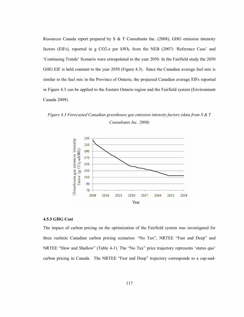
117
Resources Canada report prepared by S & T Consultants Inc. (2008), GHG emission intensity
factors (EIFs), reported in g CO2-e per kWh, from the NEB (2007) ‘Reference Case’ and
‘Continuing Trends’ Scenario were extrapolated to the year 2050. In the Fairfield study the 2050
GHG EIF is held constant to the year 2058 (Figure 4.3). Since the Canadian average fuel mix is
similar to the fuel mix in the Province of Ontario, the projected Canadian average EIFs reported
in Figure 4.3 can be applied to the Eastern Ontario region and the Fairfield system (Environment
Canada 2009).
Figure 4.3 Forecasted Canadian greenhouse gas emission intensity factors (data from S & T
Consultants Inc. 2008)
4.5.5 GHG Cost
The impact of carbon pricing on the optimization of the Fairfield system was investigated for
three realistic Canadian carbon pricing scenarios: “No Tax”, NRTEE “Fast and Deep” and
NRTEE “Slow and Shallow” (Table 4-1). The “No Tax” price trajectory represents ‘status quo’
carbon pricing in Canada. The NRTEE “Fast and Deep” trajectory corresponds to a cap-and-

118
trade policy with domestic trading only and the NRTEE “Slow and Shallow” trajectory
corresponds to a cap-and-trade policy that includes international carbon trading.
4.6 Results
The capital cost, operating cost, and GHG cost in the Fairfield expansion are presented in Table
4-6 for a range of discount rates and carbon prices to reflect possible climate change mitigating
strategies in Canada over the next 50-years. A total of six climate change mitigating scenarios
were investigated in Table 4-6 each for PVC and DCLI pipe materials. The “do nothing” climate
change mitigation approach corresponds to Scenarios 1 (PVC) and 7 (DCLI) in Table 4-6, where
costs are discounted at a rate of 8% and no carbon pricing is adopted. The strongest climate
change mitigating policy is represented by Scenario 6 (PVC) and 12 (DCLI) where the discount
rate of 1.4% proposed by Stern et al. (2006) is implemented and the NRTEE “Fast and Deep”
price trajectory is adopted.
Figure 4.4 Percent contribution of capital cost, operating cost and GHG cost to total cost for (a)
PVC and (b) DCLI pipe materials
In Table 4-6, total cost increases with decreasing discount rate and a move to a more ambitious
carbon price trajectory for both pipe materials. This is because as the discount rate is decreased,
increased weight is given to future operating and GHG emission costs. The impact of discount
rate and carbon price trajectory on the contributions of capital cost, operating cost and GHG cost

119
to total cost of the Fairfield system is indicated in Figure 4.4. With an 8% discount rate and a
“FD” carbon price trajectory, GHG costs contribute to only 7% of the total cost for PVC
(Scenario 3) and 5% for DCLI (Scenario 9). When the discount rate is reduced to 1.4% at a “FD”
carbon price trajectory, the contribution of GHG cost to the total cost reaches 21% for PVC
(Scenario 6) and 19% for DCLI (Scenario 12). Capital costs in Table 4-6 vary within a narrow
range of $100,000 for PVC pipes and $54,000 for DCLI which suggests that lowering discount
rate and increasing carbon price do not force the search algorithm to choose solutions with larger
pipe diameters in order to reduce headloss and reduce energy and GHG costs in the Fairfield
network.
Table 4-6 Capital cost, operating cost, GHG cost, and total cost of the Fairfield expansion for
PVC and DCLI pipe materials under a range of discounting and carbon pricing scenarios.
The impact of lowering the discount rate on pumping energy and total mass of GHG emissions is
examined by comparing Scenarios 1 and 4 for PVC and Scenarios 7 and 10 for DCLI (Table 4-7).
Across these scenarios, the discount rate is reduced from 8% to 1.4% while the carbon price is
fixed at $0 per tonne CO2-e. Table 4-7 indicates that discount rate does not have a significant
impact on total pumping energy and total mass of GHG emissions in the Fairfield system. For

120
PVC pipe, a decrease in discount rate from 8% to 1.4% (Scenario 1 to Scenario 4), reduces
energy use by 0.5% and GHG emissions by 0.6%. Similarly, for DCLI, a decrease in discount
rate from 8% to 1.4% (Scenario 7 to Scenario 10) reduces energy use by 0.8% and GHG
emissions by 0.5%. It is noted that the energy use in the second 25-year period is more than three
times higher than the energy use in the first 25-year period for all scenarios in Table 4-7. This
increase in energy use is owing to a near fivefold increase in average day demand (from 32 L/s in
2009 to 153 L/s in 2058) over the 50-year horizon.
Table 4-7 Energy use and mass of GHG emissions in the Fairfield expansion for PVC and DCLI
pipe materials under a range of discounting and carbon pricing scenarios.
Table 4-7 suggests that the carbon price trajectory has no significant influence on the magnitude
of pumping energy and GHG emissions for both pipe materials. At discount rates of 8% and
1.4%, moving from carbon price trajectory “NT” (No tax) to “FD” (fast and deep) produces a
change in GHG emissions that ranges from 0% to +0.7% for PVC and DCLI pipe materials.
Increasing carbon price is supposed to encourage energy conservation and lead to a decrease in
GHG emissions in a water network. However, the results in Table 4-7 indicate that GHG
emissions increase slightly with a move to a more ambitious carbon pricing trajectory. This result

121
points to the fact that carbon pricing has a negligible impact on GHG emissions in the Fairfield
network and the stochasticity of the GA search process is largely responsible for the slight
increase in GHG emissions across solutions.
The combined influence of a reduced discount rate and strong carbon price trajectory on pumping
energy and GHG emissions is assessed by comparing PVC “status quo” Scenario 1 (discount rate
= 8%; carbon trajectory = “NT”) and PVC carbon mitigating Scenario 6 (discount rate = 1.4%;
carbon trajectory = “FD”). Moving from Scenario 1 to Scenario 6 reduces pumping energy by
0.2% and GHG emissions by 0.2%. For the DCLI pipe material, moving from the “status quo”
Scenario 7 to the carbon mitigating Scenario 12 (1.4% discounting and “FD” carbon pricing)
increases pumping energy by 0.2% and GHG emissions by 0.3%. These results suggest that the
proposed discounting and NRTEE carbon-mitigation strategies have a limited impact in reducing
energy use and GHG emissions in the Fairfield system.
Table 4-8 Percent of mains duplicated, percent of mains cleaned and lined, percent of mains with
no intervention for PVC and DCLI pipe materials under a range of discounting and carbon
pricing scenarios.
The extent of pipe duplication and cleaning and lining in design Scenarios 1 through 12 are
presented in Table 4-8. The majority of duplicate pipes were installed alongside large

122
transmission mains (300 mm diameter and greater) rather than next to local distribution mains.
The results of Table 4-8 indicate that little pipe duplication and pipe cleaning and lining are
needed in the system to meet present and future demands. This suggests that there is adequate
hydraulic capacity to meet current and future demands.
4.7 Discussion
It was hypothesized that decreasing discount rate and increasing carbon pricing would guide the
optimization search to select solutions with extensive pipe duplication and more pipe cleaning
and lining relative to the “status quo” scenarios to reduce friction losses and decrease electricity
and GHG costs. However, the small variation in capital costs across all scenarios in Table 4-6
suggests that there is an adequate level of installed hydraulic capacity and that adding more
capacity does little to reduce frictional energy losses and lower electricity and GHG costs. This
observation was verified by conducting additional optimization runs for the PVC and DCLI pipe
materials with an objective function (1) that included only capital costs (new pipes, duplicate
pipes, and pipe cleaning and lining) and that excluded electricity and GHG costs. In these runs,
the capital cost was $968,114 for PVC and capital cost was $1,319,458 for DCLI. The capital
costs in these two additional runs are comparable to those found in Scenarios 1-12 of Table 4-6.
This suggests that there was adequate installed hydraulic capacity in the Fairfield network and no
additional capacity (e.g., new pipes, duplicating existing pipes, and cleaning and lining existing
pipes) was needed to offset increases in electricity cost and GHG costs driven by lower discount
rates and higher carbon prices. The exclusion of pipe-roughness growth in existing pipes also
likely discouraged the addition of duplicate pipes and the cleaning and lining of existing pipes in
the Fairfield system.

123
Other factors likely contributed to the insensitivity of electricity and GHG costs to the discount
rate and carbon pricing scenarios considered in the optimization of the Fairfield system. One
important factor is the time-declining GHG emission intensity factor used in the analysis. The
selection of discounting rate and carbon pricing can have a big impact on the weighting of GHG
costs that occur near the end of the 50-year horizon. However, a low GHG emission intensity
factor near the end of the 50-y horizon decreased the mass of GHG generated in that period and
reduced the ‘weighting force’ of discounting and carbon pricing on GHG costs. Thus the time-
declining emission factor adopted in the Fairfield study likely placed a minimal weight on GHG
costs in the objective function (1). This is in turn produced solutions with similar capital costs
each with minimal levels of pipe duplication and pipe cleaning and lining under all discounting
and carbon pricing scenarios.
The selection of a 50-year design horizon may also have played a part in the insensitivity of
electricity and GHG costs to discount rate and carbon price. Selecting a design horizon longer
than 50 years would likely increase the magnitude and weighting of electricity and GHG costs
relative to capital costs in the objective function (1). This would in turn drive the search process
to find solutions with varied capital costs and varied levels of pipe duplication and pipe cleaning
and lining under different discounting and carbon pricing scenarios.
The final factor to consider was the scope of the optimization problem. The scope of the water
distribution expansion problem was limited to include the decision variables of new and duplicate
pipe sizing and the cleaning and lining of existing pipes; tank and pump sizing and location were
excluded from the optimization problem because no needed pump and tank upgrades were
identified in the 50-year planning horizon. Despite this, the inclusion of tanks and pumps in a
network often has a large influence over energy use and GHG emissions. Had these additional
decision variables been included in the problem, larger variations in capital costs, electricity

124
costs, and GHG emission costs likely would have been observed across climate change mitigating
scenarios.
To meet the Canadian Government’s 2020 emission reduction targets, policy changes in Canada
may be centered around revised project discounting practices and a new carbon pricing
framework. The Canadian Government has set out to reduce greenhouse gas emissions by 20%
below 2006 levels by the year 2020 and by 65% below 2006 levels by the year 2050. In this
context, the proposed discount rates and carbon pricing strategies presented in this paper fail to
produce the emission-reduction levels set by the Canadian Government in the Fairfield network.
Further studies on Canadian water networks are needed to determine the effectiveness of the
proposed climate change mitigating strategies.
4.8 Summary and Conclusions
Canada may be moving closer to implementing carbon-mitigation policies that will potentially
include an economy-wide cap-and-trade carbon pricing system. This research examined the
impact of proposed GHG mitigating strategies in Canada on cost, energy use and greenhouse gas
emissions in the design and expansion optimization of the Fairfield water distribution system in
Amherstview, Ontario, Canada. The objective of the optimization approach was to minimize the
sum of capital costs associated with adding new pipes and cleaning and lining existing pipes, and
the electricity and GHG costs associated with pumping water. Results indicated that decreasing
the discount rate and moving to a more ambitious carbon pricing trajectory had no significant
impact on energy use and mass of GHG emitted in the Fairfield system. Factors that contributed
to the insensitivity of energy use and GHG emissions across climate change mitigating scenarios
included: 1) adequate hydraulic capacity in the Fairfield system to meet present and future
demands, 2) a time-declining emission intensity factor that gave minimal weighting to energy and

125
GHG costs in the objective function, 3) a relatively short design horizon of 50 years, and 4) the
exclusion of decision variables such as tank and pump location and sizing which can have a
significant impact on energy use and GHG emissions in networks. The proposed discount rates
and carbon pricing strategies presented in this paper failed to produce the emission-reduction
levels set by the Canadian Government in the Fairfield network. Further research is needed to
determine the effectiveness of the proposed climate change mitigating strategies in other water
networks in Canada.
4.9 Acknowledgments
The authors wish to thank David Thompson, P. Eng., M. J. Merritt, P. Eng., and Alex Scott
(CTech) at Loyalist Township for their contributions to the development of this paper. This
research was financially supported by Queen’s University and the Natural Sciences and
Engineering Research Council (NSERC).
4.10 References
Ambrose, M. D., Salomonsson, G. D., and Burn, S. (2002). “Piping Systems Embodied Energy
Analysis.” CMIT Doc. 02/302, CSIRO Manufacturing and Infrastructure Technology,
Highett, Australia.
Bank of Canada. (2009). “Monthly And Average Of Exchange Rates.”
(http://www,bankofcanada.ca: Accessed August 3, 2009).
Bhandari, D., Murphy, C.A., Pal, S.K. (1996) “Genetic Algorithm with Elitist Model and Its
Convergence”, International Journal of Pattern Recognition and Artificial Intelligence,
10(6), 731-747.

126
Boardman, A. E., Moore, M. A., and Vining, A. R. (2008). Social Discount Rates for Canada.
John Deutsch Institute Conference: Discount Rates for the Evaluation of Public Private
Partnerships. Kingston, Ontario, Canada.
Burgess, D. F. (1981). “The Social Discount Rate For Canada: Theory And Practice.” Canadian
Public Policy, 7(3), 383 – 394.
CH2M Hill. (2007). Fairfield Water Storage Project – Final Report. CH2M Hill, Ottawa.
Cline, W. R. (1992). The Economics of Global Warming. Institute for International Economics,
Washington, D.C.
Clarke, A., Grant, N., Thornton, J. (2009). Quantifying the energy and carbon effects of water
saving. Environment Agency, Rotterdam, UK.
Cuddihy, J., Kennedy, C., Byer, P. (2005). “Energy Use In Canada: Environmental Impacts And
Opportunities In Relationship To Infrastructure Systems.” Can. J. Civ. Eng., 32, 1-15.
Dandy, G., Roberts, A, Hewitson, C., and Chrystie, P. (2006). “Sustainability Objectives For The
Optimization Of Water Distribution Networks.” 8th Annual Water Distribution Systems
Analysis Symposium, Cincinnati, Ohio, August 27-30, 2006.
Dandy, G., Bogdanowicz, A., Craven, J., Maywald, A., Liu, P. (2008). “Optimizing the
Sustainability of Water Distribution Systems.” WDSA 2008, South Africa, August 17-21,
2008.
Dennison, F. J., Azapagic, A., Clift, R., and Colbourne, J. S. (1999). “Life Cycle Assessment:
Comparing Strategic Options For The Mains Infrastructure—Part I.” Water Sci. Technol.,
39(10–11), 315–319.

127
Electric Power Research Institute. (1994). Energy Audit Manual for Water/Wastewater Facilities.
EPRI, Palo Alto, CA.
Engineering News Report (ENR). (2009). “Construction Cost Index History.”
(http://enr.construction.com/: Accessed August 3, 2009).
Environment Canada (2009). National Inventory Report 1990-2007: Greenhouse Gas Sources and
Sinks in Canada. Library and Archives Canada Cataloguing in Publication, Gatineau,
Quebec.
Fearnside, P., M. (2002). “Time Preference In Global Warming Calculations: A Proposal For A
Unified Index.” Ecological Economics, 41(1), 21-31.
Filion, Y. R., MacLean, H. L., and Karney, B. W. (2004). “Life-Cycle Energy Analysis Of A
Water Distribution System”, Journal of Infrastructure Systems, 10(3), 120–130.
Fire Underwriters Survey (FUS). (1999). Water Supply for Public Protection. CGI Group Inc.,
Markham.
Ghimire, S. R., and Barkdoll, B. D. (2007). “Incorporating Environmental Impact Decision
Making For Municipal Drinking Water Distribution Systems Through Eco-Efficiency
Analysis.” Proc., EWRI-2007, ASCE, Reston, Va., 1–10.
Hasselmann, K., Hasselmann, S., Giering, R., Ocana, V., and Storch, H. V. (1997). “Sensitivity
Study of Optimal CO2 Emission Paths Using a Simplified Structural Integrated
Assessment Model (SIAM).” Climate Change, 37(2), 345-386.
Herstein, L.H., Filion, Y.R., Hall, K. (2009). “Evaluating Environmental Impact in Water
Distribution System Design.” Journal of Infrastructure Systems, 15(3), 241-250.

128
Herstein, L.H., Filion, Y. R., and Hall, K. (2010). “Evaluating The Environmental Impacts Of
Water Distribution Systems Using EIO-LCA-Based Multi-objective Optimization.”
Journal of Water Resources Planning and Management.
Hudson, W. D. (1966) “Studies Of Distribution System Capacity In Seven Cities.” Journal of
American Water Work Associations, 58 (2) 157-164.
Jenkins, G.P., and Kuo, C.Y. (2007). The Economic Opportunity Cost of Capital for Canada – An
Empirical Update. Queen’s Economics Department Working Paper No. 1133.
Larson, T. E. and Sollo, F. R. (1967) “Loss In Water Main Carrying Capacity.” American Water
Work Associations, 59(12), 1565–1572.
Lundie, S., Peters, G. M., and Beavis, P. C. (2004). “Life Cycle Assessment For Sustainable
Metropolitan Water Systems Planning.” Environ. Sci. Technol., 38, 3465–3473.
Lundie, S., Peters, G. M., and Beavis, P. C. (2005). “Quantitative Systems Analysis As A
Strategic Planning Approach For Metropolitan Water Service Providers.” Water Sci.
Technol., 52(9), 11–20.
Majumdar, J., Bhunia, A.K. (2007) “Elitist Genetic Algorithm For Assignment Problem With
Imprecise Goal”, European Journal of Operational Research, 177(2), 684-692.
National Energy Board (NEB). (2007). Canada’s Energy Future Reference Case and Scenarios to
2030: An Energy Market Assessment. National Energy Board Publications, Calgary.
National Round Table on the Environment and the Economy (NRTEE). (2007). Getting to 2050:
Canada’s Transition To a Low-emission Future. Library and Archives Canada Cataloguing
in Publication, Ottawa.

129
National Round Table on the Environment and the Economy (NRTEE). (2009). Achieving
2050:A Carbon Pricing Policy For Canada. Library and Archives Canada Cataloguing in
Publication, Ottawa.
Nordhaus, W., D. (1991). “To Slow Or Not To Slow: The Economics Of The Greenhouse
Effect.” The Economic Journal, 101(July), 920-937.
Ontario Energy Board (OEB). (2008). Regulated Price Plan Price Report. Queens Printer for
Ontario, Toronto.
Rossman, L. A. (2000). EPANET2 User’s Manual. US EPA, Washington, D.C.
S & T Consultants Inc. (2008). 2008 GHGenius Update. Natural Resources Canada, Ottawa.
Stern, Nicholas, Peters, S., Bakhshi, V., Bowen, A., Cameron, C., Catovsky, S., Crane, D.,
Cruickshank, S., Dietz, S., Edmonson, N., Garbett, S. L., Hamid, L., Hoffman, G., Ingram,
D., Jones, B., Patmore, N., Radcliffe, H., Sathiyarajah, R., Stock, M., Taylor, C., Vernon,
T., Wanjie, H., and Zenghelis, D. (2006). Stern Review: The Economics of Climate
Change. HM Treasury, London.
Stokes, J., and Horvath, A. (2006). “Life Cycle Energy Assessment Of Alternative Water Supply
Systems.” Int. J. Life Cycle Assess., 11(5), 335–343.
Treasury Board of Canada Secretariat (TBS). (2007). Benefit-Cost Analysis Guide – Interim
Report. Treasury Board of Canada Secretariat, Ottawa.
Walski, T. M. (1986). “Predicting Costs Of Pipe Cleaning And Lining Projects.” Journal of
Transportation Engineering, 1123(3), 317 – 327.
130
Wu, W., Simpson, A. R., and Maier, H. R. (2008). “Multi-Objective Genetic Algorithm
Optimization Of Water Distribution Systems Accounting For Sustainability.” 10th Annual
Symposium on Water Distribution Systems Analysis, South Africa, August 17-20.
Wu, W., Maier, H. R., and Simpson, A.R. (2009). “Single-Objective Versus Multi-Objective
Optimization Of Water Distribution Systems Accounting For Greenhouse Gas Emissions
By Carbon Pricing.” Journal of Water Resources Planning and Management, 136(5), 555-
565.
Wu, W., Simpson, A.R., and Maier, H. R. (2010). “Accounting for Greenhouse Gas Emissions in
Multi-Objective Genetic Algorithm Optimization of Water Distribution Systems.” Journal
of Water Resources Planning and Management, 136(2), 146-155.

131
Chapter 5
Event-Based Approach to Optimize the Timing of Water Main
Rehabilitation with Asset Management Strategies
5.1 Abstract
Municipalities with limited budgets will have to rehabilitate a large stock of deteriorated water
mains in the coming decades. There is an opportunity to reduce rehabilitation costs through
optimization and asset management strategies. The aim of this paper is to present a new event-
based approach to optimize the timing of water main rehabilitation. The approach incorporates a
new sparse gene-coding scheme and covers the full range of decision variables such as pipe
replacement, pipe duplication, pipe lining, the installation of new pipes, and asset management
strategies (e.g., budget constraint and discounts). The new approach was applied to the Fairfield
water network. The results suggest that applying a budget constraint prohibited the search process
from investing early and heavily in pipe rehabilitation with a resulting increase in cost linked to
pipe leakage, pipe breaks, and energy use. Applying discounts decreased capital and operational
costs and favored pipe lining over pipe replacement and duplication. A sensitivity analysis
showed that water demand, leakage and break growth rates can have a moderate to significant
impact on capital and operational costs.
Keywords: water distribution systems, rehabilitation, asset management, multi-objective
optimization, pipe breaks, pipe leakage, pipe aging.

132
5.2 Introduction
Most water distribution systems in North America are old and in need of rehabilitation. An
estimated $325 billion is needed to rehabilitate drinking water systems in the United States (Deb
et al. 2002) to maintain current service levels. A Canadian study has indicated that $11.5 billion
should be spent over the next 15 years to upgrade municipal water distribution systems (CWWA
1997). In North America, water distributions systems lose water at an average rate of 20-50%
(Brothers 2001) and at comparable rates in Europe (European Environment Agency 2010). Water
loss through leaks and pipe roughness growth in deteriorated pipe account for low pressures,
increases in energy costs, and higher repair costs in water distribution networks. Municipalities
are faced with the prospect of rehabilitating and replacing a large stock of deteriorated water main
assets with capital budgets that are increasingly stretched to their limit. In this context,
municipalities have started to examine optimization and asset management strategies as means to
reduce the cost of water main asset rehabilitation and replacement.
Research in the last 30 years has focused on developing models to optimize the timing of pipe
replacement and rehabilitation in networks. Shamir and Howard (1979) and Walski and Pelliccia
(1982) were the first to propose the exponential break model to forecast pipe break rates over a
future time horizon. Arulraj and Suresh (1995) developed a significance index to prioritize pipe
rehabilitation. Kleiner et al. (1998) proposed a new optimization framework that made use of the
exponential break model in which break rate was modeled deterministically as a function of age.
In their approach, both network economics and hydraulic capacity were analyzed simultaneously
over a pre-defined time horizon. Goulter and Kazemi (1998) studied the effect of spatial and
temporal clustering on pipe failure rates. They showed that historical failures in a location of
interest are an important predictor of future failures in the same location. Dandy and Engelhardt
(2001) applied genetic algorithms (GAs) to optimize the pipe replacement scheduling of the

133
Adelaide water distribution system and to minimize the overall cost of the project. They showed
that GAs are able to identify which pipes to replace when an available budgetary constraint is
considered in the decision making procedure. Burn et al. (2003) developed a pipeline asset and
risk management system to prioritize the replacement of pipe groups. The model was used to
predict failure rates for individual pipes rather than for cohorts of pipes. Nafi et al. (2008)
developed a decision support model that considers available financial resources in pipe renewal
scheduling. The authors used Cox’s proportional hazard model (PHM) to forecast pipe failure and
combined it with multi-objective optimization to enhance the network reliability and reduce
failure occurrences.
Multi-objective approaches to optimize the rehabilitation timing of water main assets have also
been suggested. Halhal et al. (1999) used a messy genetic algorithm to solve the rehabilitation
timing problem. The model was applied to a simple case study in which they maximized benefits
of improved system performance and minimized the costs under an available budget constraint.
Halhal et al. (1999) also examined the sensitivity of the optimal solution to uncertainties in
interest rate and inflation rate. Dandy and Engelhardt (2006) proposed a multi-objective
framework to minimize the rehabilitation costs and maximize network reliability simultaneously.
In their work, the economic costs of rehabilitation were converted to the present value and
reliability was measured as the expected number of customer interruptions per year. Their work
provided the starting point that can be extended to include other performance measures which
affect customers’ level of service. Dridi et al. (2008) used and compared several evolutionary
optimization techniques including IGA, NPGA-II, and NSGA-II to schedule water pipe renewal
for short planning periods. Their results confirmed that using evolutionary algorithms could be
useful to solve the pipe renewal scheduling problem. In particular, they recommended the use of
NSGA-II to optimize large networks. Nafi and Kleiner (2010) developed a model to optimize the

134
timing of pipe renewal in a distribution network. Their model included discounts that account for
the adjacency of infrastructure works to the newly installed pipes and volume discounts on large
quantities of purchased pipe for installation in networks. The Nafi and Kleiner (2010)
optimization model minimizes cost that include pipe replacement and break repair and maximizes
the available budget. The Nafi and Kleiner model does not account for pipe roughness growth and
leakage which often drive the search process since the operation cost is often the most significant
component of the total cost.
Water distribution system rehabilitation optimization has been addressed in the literature mainly
by focusing only on pipe replacement and, in some rare cases, pipe lining. This has been done
mostly to simplify what is a complex optimization problem. In reality, utility owners and
managers select among a wider decision domain which includes pipe duplication, pipe
replacement, a set of pipe lining technologies (e.g., cement-mortar lining, cured-in-place liners),
and installing new pipes in areas slated for new growth. Eliminating decision options to simplify
the problem sacrifices the practicality of the approach.
Further, previous approaches have attempted to reduce the complexity of the rehabilitation
problem by grouping pipes in cohorts or groups and applying replacement scheduling decisions to
all pipes in a cohort. In the cohort method, a decision is made for a group of pipes which share
some common properties. The number of decisions needed to schedule rehabilitation is fewer in
this approach. However, since all pipes in the same group are treated in exactly the same way,
these algorithms cannot guarantee that a decision is optimal for each individual pipe in the group.
Another limitation of previous approaches is the assumption that an individual pipe should be
replaced strictly if its maintenance cost (e.g., break repair cost) is greater than the replacement
cost (Nafi and Kleiner 2010, 2011) without considering system-wide effects. Replacing an

135
individual pipe strictly based on its maintenance cost and regardless of the effect of this single
pipe on the financial analyses of the entire system is neither accurate nor will it guarantee that the
final solution will be optimal.
Unlike previous models, the optimization model presented in this paper selects among the fullest
range of rehabilitation and/or replacement options that include: the replacement of existing pipes
with new pipes, the lining of existing pipes, the duplication of existing pipes while making it
possible to apply the fullest range of rehabilitation options to the primary pipe, and the
installation of new pipes in new growth areas. Unlike previous models (Nafi and Kleiner 2010,
2011), the model presented in this paper considers the fullest range of commercially-available
pipe diameters. The financial and hydraulic performances of each pipe are evaluated annually in
the system and in combination with other pipes. Time-varying pipe properties such as the Hazen-
Williams ‘C’ factor, break rates, and leakage rates are considered in the model. The model is used
to perform an extended period simulation (e.g., 24 hours) in each year of the planning horizon to
construct a complete hydraulic ‘picture’ of the system and to better estimate water loss and
energy use. The model is used to perform fire simulations at critical nodes in a system at the
beginning, middle, and the end of planning period. Previous rehabilitation studies (Halhal et al.
1999, Dandy and Engelhardt 2006, Nafi and Kleiner 2010, Kleiner and Nafi 2011) have not
incorporated as extensive a hydraulic analysis as was done in this research.
The paper presents a new event-based multi-objective optimization algorithm that determines the
optimal allocation of financial resources and optimal scheduling of water main rehabilitation in
water distribution networks. The new optimization model accounts for annual capital and
operating budgets and incorporates realistic asset management strategies. The event-based model
incorporates a novel sparse gene-coding scheme with small computational and memory
requirements that assigns a unique sequence of rehabilitation events (rehabilitation time and type)

136
to each individual pipe independently of all other pipes in the network. (This is in contrast to
previous models where a limited number of rehabilitation schedules are applied to all pipes in an
a priori manner.) The model can characterize the hydraulic and cost performance of the unique
rehabilitation schedules assigned to each pipe by simulating breaks, leakage, pipe-roughness
aging, and hydraulic conditions in the network. The optimization model was applied to the real-
world Fairfield water distribution system in southeastern Ontario, Canada, which has
approximately 400 pipes and supplies water to approximately 15,000 people. The algorithm was
run on a 120 parallel core high performance computing cluster with the Message Passing
Interface (MPI) to distribute the computational load among computing nodes (Roshani et al.
2012c).
The chapter is organized as follows. First, the rehabilitation optimization problem is
mathematically defined. Second, the Fairfield case study is described. Third, the new algorithm is
used to optimize the timing of water main rehabilitation and replacement in the Fairfield system
under four asset management scenarios. Fourth, a sensitivity analysis is performed to determine
the sensitivity of capital and operational costs to variations in uncertain parameters such as water
demand, leakage, and pipe roughness.
5.3 Problem Definition
The multi-objective optimization problem seeks to find the optimal timing of water main
rehabilitation and replacement that minimizes the present value of capital and operational costs of
the network as detailed in the objective functions (1)-(2). A fast-elitist non-dominated sorting
genetic algorithm (NSGA-II) by Deb et al. (2002) was used to search the large decision space
efficiently and minimize two objectives:

137
( )DR
T
t
np
pptptptpt NPLCDCRCPVCCMinObj
+++== ∑∑
= =0 1,,,,)(1 (1)
( )DR
T
t
np
p
T
ttptpt ECBCLkCPVOCMinObj
++== ∑∑ ∑
= = =0 1 0,,)(2 (2)
in which CC is the capital cost, OC is the operational cost, PV is the present value of the costs,
DR is the discount rate, t is time in years, T is the planning horizon of the project, p is the pipe
number, np is the maximum pipe number, ptRC , is replacement cost for the pth pipe in the tth
year, ptDC , is pipe duplication cost, ptLC , is lining cost, ptNP , is the new pipe cost, ptLkC , is the
cost of lost water to leakage, ptBC , is break repair cost, and tEC is the cost of electricity to pump
water. The optimization is also subject to an annual budget constraint such that annual
expenditures cannot exceed an annual budget ceiling tAB for year t in the planning period. Since
the cost of lost water to leakage is not a budget line item, it has been eliminated from the annual
costs in the budget constraint (3)
( ) t
np
ptptpppp ABECBCNPLCDCRC ≤+++++∑
=1, (3)
The usual nodal continuity and loop energy conservation constraints are satisfied externally with
the network solver EPANET2 (Rossman 2000). The optimization is also subject to minimum
pressure and fluid velocity constraints under peak demands. The decision variables are the time,
the type, and the place of rehabilitation decisions. Possible types of rehabilitation interventions
include the diameter of a pipe being replaced, the diameter of a pipe being duplicated, the
diameter of a new pipe in an area slated for future growth, and the type of lining technology used.
It also includes the same decisions for the pipe installed as a duplicated pipe.

138
5.4 Event-Based Rehabilitation: A New Approach to Gene Coding
To simulate a sequence of rehabilitation events for a single pipe in the water main rehabilitation
timing problem, the traditional approach is to use one gene to represent each year of the planning
horizon. For instance, 50 genes are required to simulate a rehabilitation event in each year of a
50-year planning period in a single pipe. If pipe duplication is also included in the optimization,
the number of genes must be doubled to simulate the rehabilitation events linked to the duplicated
pipe added in the system. In practice, most of these genes will have zero values in the optimal
solution since no rehabilitation activities take place in most years. For example, after replacing an
existing pipe with a new pipe, there is typically no need to replace or rehabilitate the pipe for at
least another 20-30 years and thus all the genes that represent the intervening 20-30 years are set
to zero. This dramatically increases the computational and memory requirements for solving the
water main rehabilitation timing problem. Moreover, based on schema theorem (Holland 1992),
having these zero-valued (dormant) genes can greatly decrease the speed of convergence to the
optimal solutions. This is due to the fact that the zero-valued genes increase the number of
decision variables and hence the search space unnecessarily.
Figure 5.1 Encoded genes in a chromosome for a single pipe and its duplicate.

139
The new gene coding adopted in this research is indicated in Figure 5.1. The chromosome
structure indicated in Figure 5.1 applies to a single pipe, henceforth called the “main pipe”, and
an adjacent duplicate pipe over a fixed planning horizon. A variable called Maximum Number of
Events (MNE) represents the maximum number of rehabilitation events expected over the
planning period for the main pipe and the duplicate pipe. Considering a lag time of 20-30 years
between rehabilitation interventions and a planning horizon of 50 years, typical MNE values
could range between 3 and 5. In other words, a pipe and its duplicate could be rehabilitated 3 to 5
times over a 50-year planning horizon.
In Figure 5.1, each rehabilitation event applied to the main pipe and its duplicate (if it is needed)
is described with four gene identifiers. The first gene identifier “Event time (main pipe)” denotes
the timing of the rehabilitation event applied to the main pipe. The second gene identify “Main
pipe event type” denotes the type of rehabilitation applied to the main pipe. The third gene
identifier “Event time (duplicate pipe)” denotes the timing of rehabilitation applied to the
duplicate pipe. The fourth gene identifier “Duplicate pipe event type” denotes the type of
rehabilitation applied to the duplicate pipe. For example, in Figure 5.1 the first rehabilitation
event (Event 1) has four gene identifiers. The first gene identifier “9” means that the main pipe is
replaced in Year 9 of the planning horizon. The second gene identifier “3” means that the main
pipe will be replaced with a new pipe with a new 250 mm diameter. The third and fourth gene
identifiers “0” and “0” mean that in Year 0, no duplicate pipe is installed (Do nothing - “0”). In
Figure 5.1, for an MNE of 5 events over a 50-year planning horizon, the new gene coding
approach of this research produces a chromosome with 20 genes. By comparison, the traditional
gene coding method of previous models (Dandy and Engelhardt 2006; Nafi and Kleiner 2010,
Kleiner and Nafi 2011) would require 100 genes (2 genes for the main pipe and the duplicate pipe
in each year of the 50-year planning horizon). The new approach of this research can thus reduce

140
the chromosome length by 80% and thus save a significant amount of computer memory and
increase the speed of convergence.
5.5 Asset Management Strategies
Budget limitations often force utility decision makers to employ rehabilitation strategies that will
allow them to manage their assets in the most cost-effective way. Synchronizing several
municipal maintenance projects (e.g., roadwork with pipe replacement and rehabilitation), and
aggregating rehabilitation projects together to get a discounted price on materials and labour are
two common approaches used to cut costs (Nafi and Kleiner 2010). The new model accounts for
savings achieved through synchronizing road reconstruction work with water main replacement
or rehabilitation (henceforth called the infrastructure adjacency discount) and discounts achieved
on the purchase of large quantities of water main pipe (henceforth called the economies of scale
discount). The infrastructure adjacency and economies of scale discounts are indicated in (4)
( ) pppp ACConDAdjDDAC ×−×= 1 (4)
in which pDAC is the discounted rehabilitation activity cost for pipe p . The actual pipe
rehabilitation cost pAC in (4) is reduced by the infrastructure adjacency discount, pAdjD , and
the quantity discount pConD . The infrastructure adjacency discount pAdjD is applied to all
water main rehabilitation activities if they are carried out in the same year of road construction or
re-construction work in which the pipe is located. The quantity discount pConD is applied to
new pipes installed, old pipes replaced, and old pipes duplicated projects completed in the same
year and purchased on a volume basis. This means the water main rehabilitation activities should
be performed on pipes which have at least one node in common and should occur in the same

141
year to be considered for quantity discounting (Nafi and Kleiner 2010). The quantity discount is
calculated from the schedule in (5)
( )( )
<
≤<−
−
≤
=
t
tt
t
p
llConD
lllll
llConDll
ConD
maxmax
maxminminmax
minmax
min
,
,
,0
(5)
in which tl is the total pipe length to be replaced or rehabilitated, maxConD is the maximum
value of the quantity discount, minl , maxl are minimum and maximum pipe length quantities that
determine the minimum and maximum quantity discounts, as defined by the supplier (contractor).
A graphical illustration of (5) is shown in Figure 5.2. This figure indicates that if the length of
pipe to be rehabilitated is less than minl , the quantity discount is zero. If the length of pipe to be
rehabilitated is more than lmax, then the quantity discount is set to its maximum level. If the
rehabilitation length falls between minl and maxl , the quantity discount will be between 0 and
maxConD in (5).
Figure 5.2 Effect of pipe length on quantity discount.

142
5.6 Model Implementation
The non-dominated sorting genetic algorithm (NSGA-II) was combined with the hydraulic solver
EPANET2 (Rossman 2000), a pipe-aging model, a pipe leakage model and a pipe break
forecasting model to solve the water main rehabilitation timing problem. Figure 5.3 indicates a
flowchart of the OptiNET pipe rehabilitation optimization model which makes use of parallel
computing to decrease computational time.
Figure 5.3 Flow chart of OptiNET optimization model.

143
In Figure 5.3, an initial random population of solutions is generated. The population of solutions
is sent to the hydraulic model, pipe aging, leakage, and pipe break models for hydraulic and
economic evaluation. In each year of the planning horizon, the new pipe replacement and
rehabilitation activities are applied to the layout of the network. Based on the location and
quantity of these new and rehabilitated pipes relative to other public works infrastructure (e.g.,
roads, other utilities), quantity and infrastructure adjacency discounts in (4)-(5) are calculated.
Pipe roughness and pipe leakage are updated with pipe aging and pipe leakage models (discussed
below) specified by the user. The EPANET2 hydraulic solver is then run to evaluate the hydraulic
performance of the network for the new pipe layout, and the pipe roughness and pipe leakage
conditions applied. The break repair cost is estimated for the current year with a break forecasting
model specified by the user.
The objective functions (1)-(2) are updated and errors are calculated for the current year. The
hydraulic and economic evaluations are repeated in this manner for all n years of the planning
period. The objective functions and errors computed over n years of the planning period for all
solutions in the population are then used by the NSGA-II to perform crossover, mutation, and
selection operations to select the next population of solutions. Successive populations are
generated and evaluated until a stopping criterion is satisfied.
5.7 Fairfield Water Distribution Network
The Fairfield system provides drinking water to the community of Amherstview and Odessa in
southeastern Ontario which have a combined population of approximately 15,000 people. Figure
5.4 indicates the all-pipes model of the system with 405 pipe segments and Table 5-1 indicates
the material and age distribution of the pipes in the Fairfield network.

144
Figure 5.4 Fairfield water distribution system.
PVC pipes were used to replace old pipes or to duplicate them as specified by Loyalist Township.
The unit prices of PVC pipes were obtained from a Canadian pipe distributor and are indicated in
Table 5-2. Pipe cleaning and cement-mortar lining costs were estimated by inflating costs from
Walski (1986) to 2010 dollars. Detailed cost calculations can be found in Roshani et al. (2012a).
Table 5-1 Pipe material and age distribution in Fairfield system.

145
Table 5-2 Unit costs of commercially-available PVC pipes and DI pipes cleaning and lining costs
(adapted from Walski 1986).
The average day demand in the Fairfield network is 32 L/s. The water demand at the end of the
20-year planning horizon was projected with annual growth rates reported in Table 5-3 and
provided by Loyalist Township (CH2M Hill 2007). Two future network expansions are planned
by Loyalist Township. The first expansion located in the western part of the network (indicated in
Figure 5.4 as a grey-shaded area) will be completed in the first 10 years of the planning period
and the second expansion, located in the northern part of the network, will be completed at the
end of the 20-year planning horizon. Loyalist Township has an annual budget of $850,000 / yr for
capital and operational expenditures (Thompson 2011).
The hydraulic performance (maximum velocity and minimum pressure limit) of the Fairfield
network was evaluated under average day and peak demands. The maximum velocity constraint
was evaluated under maximum hour and/or maximum day + fire demand for each year of the 20-
year rehabilitation planning period. Average day demand was modeled as an extended period
simulation (EPS) for 24 hours with an average day diurnal pattern. The average day demand EPS
was performed for each year of the planning period. Maximum hour demand simulations were

146
performed at Year 0, Year 10, and Year 20 of the planning period. Maximum day + fire
simulations were performed and pressures were observed at 2 critical nodes (J-514 and J-551 in
Figure 5.3) at Years 0, 10, and 20. A needed fire flow of 33 L/s was adopted in accordance with
Fire Underwriters Survey (FUS) guidelines (FUS 1999). Therefore the hydraulic conditions of
each solution was evaluated on the basis of twenty 24-hour extended period simulations, three
maximum hour demand simulations, and six maximum day demand + fire simulations.
Table 5-3 Projected annual growth rates and current and projected water demands in the Town
of Amherstview.
Water Use Land Use (%)Annual
Growth Rate (%)
2010 Present Water Demand
(L/s)
2030 Projected Water Demand
(L/s)
Residential 68 3.5 20 40Multi-residential 18 3.5 6 12Commercial 2 2 1 2Institutional 8 2 2 3.7Industrial 10 1 3 4.1New Industrial - - 0 8.8Total 100 32 70.6
5.7.1 Pipe Leakage Model
A number of models have been proposed in the literature to forecast leakage in deteriorated pipes.
Among these models, the approach by Germanopoulos (1985) that was later adapted by Alvisi et
al. (2009) was used in this study to forecast water loss in the Fairfield network. This approach
was selected for its simplicity and its accuracy in estimating lost water and for its parsimonious
data requirements. The approach assumes that the leak area (percent of the pipe wall surface area)
increases over time as a function of pipe age and that it follows an exponential trend as in (6)
147
tpp eld βυπ=Ω (6)
in which Ω is the percent of open surface area in a pipe, π = pi constant, pd = pipe diameter, pl
= pipe length, υ and β are two exponential components, and t = pipe age (year). While υ and
β may vary with pipe diameter and material and even the type of pipe installation (Martinez et
al. 1999), they have been assumed to be the same for all pipe segments in the Fairfield system
since there is no data available for these variables. (It is noted that both these variables are subject
to a sensitivity analysis presented later in this paper.) Both of these variables were calibrated
based on water loss measurements provided by Loyalist Township. The calibration was
performed for the period 1998-2003 in which no rehabilitation activities (pipe replacement and
lining) were reported. The calibrated leak model parameters were found to be υ = 4 × 10⁻⁷ and
β =0.13 for the Fairfield network.
5.7.2 Break Model
A total of 94 pipe break incidents were reported by Loyalist Township in the period 1982-2011.
Break distribution by pipe material is indicated in Table 5-4. The time-exponential break model
of Shamir and Howard (1979) was used to project the number of breaks in each pipe. The Shamir
and Howard (1979) forecasting model was used in this research because it is practical and has
been used extensively in the past to generate reasonable forecasting results. This model assumes
that number of breaks will increase exponentially with pipe age as in (7).
teNbr βα 0= (7)
in which Nbr is the future break rate, 0α = initial break rate (break/year/km), β = break
growth rate (break/year), and t = time (year). The values of 0α and β were calculated for cast
iron (CI) and ductile iron (DI) pipe materials based on the records provided by Loyalist

148
Township. Break records for Asbestos Cement (AC) and Polyvinyl Chloride (PVC) pipes were
scarce and so values near the lower limit of the proposed range in the literature were assumed for
0α and β in AC and PVC pipes (Shamir and Howard 1979; Walski and Pelliccia 1982; Kleiner
and Rajani 1999; Mailhot et al. 2003). The effects of these values on the Pareto front were also
examined in the sensitivity analysis of the paper. Table 5-4 indicates the calibrated and assumed
values for the pipe break exponential models applied to the Fairfield system.
Table 5-4 Break distribution by pipe material and exponential model values.
5.7.3 Pipe Roughness Growth Model
The roughness growth model of Sharp and Walski (1988) has been used extensively in the
research literature to forecast reductions in the Hazen-Williams ‘C’ factor in aging pipe. Since the
Sharp and Walski (1988) roughness growth model is unique in the literature, it was adopted in
this study to forecast Hazen-Williams ‘C’ factors in CI and DI pipes in the Fairfield network.
Flow test data were used to estimate the Hazen-Williams ‘C’ factor values of existing water
mains in the network (CH2M Hill 2007). Average ‘C’ factor values of 55 for cast iron, 120 for
concrete, 120 for ductile iron and 150 for PVC pipes were found. Given the inability of the Sharp
and Walski model to forecast roughness growth in PVC and AC pipe, the ‘C’ factors for these

149
pipe materials were assumed constant for the planning period. The assumption of constant ‘C’ is a
conservative assumption with respect to energy use.
5.8 Asset Management Scenarios and Results
Four scenarios were defined to investigate the impact of different water main asset management
strategies on capital and operational costs in the Fairfield network. In Scenario 1 (Scn. 1), both
infrastructure adjacency and quantity discounts were applied in conjunction with the annual
budget constraint. In Scenario 2 (Scn. 2), the discounts were applied while the annual budget
constraint was not applied. In Scenario 3 (Scn. 3), both the adjacency and quantity discounts and
the annual budget constraint were not applied. In Scenario 4 (Scn. 4), the infrastructure adjacency
and quantity discounts were not applied, while the budget constraint was applied.
5.8.1 Pareto-Fronts of Scenarios 1 Through 4
The Pareto fronts generated in the four scenarios are indicated in Figure 5.5. This figure indicates
that the Scenario 2 front (discounts applied, budget constraint not applied) has the lowest capital
cost and operational costs, while the Scenario 4 front (discounts not applied, budget constraint
applied) has the highest costs. The application of the budget constraint and the adjacency and
quantity discounts largely accounts for the difference in cost between these two fronts. Scenario 2
has low capital costs because it benefits from adjacency and quantity discounts, while Scenario 4
has higher capital costs because no such discounts are available. The removal of the budget
constraint in Scenario 2 allows the optimization engine to make “up-front” capital investments to
replace and rehabilitate the large stock of old, deteriorated water mains in the Fairfield system.
This “up-front” capital investment at the beginning of the planning period is not capped by the
budget constraint and allows the municipality to lower operational costs in the system in
subsequent years – mostly from reduced leakage and reduced energy use for pumping.

150
Conversely, applying the budget constraint in Scenario 4 limits the “up-front” capital investments
to the available annual funds (as set by the budget). The rehabilitation of the old, deteriorated
stock of pipes must be deferred to subsequent years which increases operational costs from
leakage loss and pumping.
Figure 5.5 Pareto fronts generated in asset management Scenarios 1 through 4.
The capital and operational costs of solutions located at opposite ends of the Pareto fronts in
Figure 5.5 were examined and compared. In Figure 5.5, select solutions in distinct regions of each
Pareto front are indicated with a circle. These solutions are the minimum capital cost solutions
(left side of fronts), the minimum operational cost solutions (right side of fronts), and the
minimum total cost solutions (at or near the elbow of the fronts). In Table 5-5, the minimum
capital cost solution is identified with the hyphenated identifier “-1” (e.g., Scn. 1-1), the

151
minimum operational cost solution is identified with “-2” (e.g., Scn. 1-2), and the minimum total
cost solution is identified with “-3” (e.g., Scn. 1-3).
Table 5-5 Average annual costs, present value capital costs, present value operational costs, and
present value total cost for asset management Scenarios 1 through 4.
PV Operational
CostBreak Leak Energy ($M)
Scn. 1-1 2 X X X 49.5 276.6 44.9 3.13 4.68 7.81
Scn. 1-2 3
X X X 29 174.8 43 4.35 2.61 6.96
Scn. 1-3 4X X X 38.6 218.6 43.7 3.52 2.99 6.51
Scn. 2-1 X X 63.8 366.4 45.4 3.05 4.42 7.47Scn. 2-2 X X 17.4 82.9 40 4.52 1.64 6.16Scn. 2-3 X X 15.8 101.3 39.3 3.81 1.72 5.53Scn. 3-1 56.5 379.5 46 3.11 4.35 7.47Scn. 3-2 19.1 103.2 39.2 5.45 1.85 7.29Scn. 3-3 24.1 121.9 40.2 4.03 1.96 5.98Scn. 4-1 X 59.5 379.4 46.5 3.29 4.5 7.79Scn. 4-2 X 34.2 196.8 42.3 4.66 2.9 7.56Scn. 4-3 X 37.1 226.7 44.4 3.72 3.14 6.86
Average Annual Cost ($1,000) PV Capital
Cost ($M) 1PV Total Cost ($M)Solution
Adjacency Discount
Quantity Discount
Budget Limit
1. $M = millions of dollars 2. Scn. 1-1 denotes the minimum capital cost solution on the Scenario 1 front (from Figure 5.5). 3. Scn. 1-2 denotes the minimum operational cost solution on the Scenario 1 front (from Figure 5.5). 4. Scn. 1-3 denotes the minimum total cost solution on the Scenario 1 front (from Figure 5.5).
Table 5-5 indicates that minimum capital cost solutions (“-1”) have higher average annual
operational costs (break repair, leakage, and energy) than minimum operational cost solutions (“-
2”). This is owing to the fact that in minimum capital cost solutions (“-1”), the search process
makes minimal capital investments to replace and rehabilitate the old CI pipe stock in the
Fairfield network to keep the capital costs low. As a result, the unimproved CI pipe stock breaks
frequently, has a high leakage level, and induces high frictional losses in the system which
account for the high annual operational costs. By contrast, in minimum operational cost solutions

152
(“-2”) continuous investments in rehabilitation are made throughout the planning period to keep
operational costs low.
5.8.2 Impact of the Budget Constraint and Discounts on Capital and Operational Costs
The influence of the budget constraint on average annual costs (breaks, leaks, and energy) in the
four scenarios was examined. Scenario 1 where the budget constraint is imposed was compared to
Scenario 2 where it is not (both scenarios include adjacency and quantity discounts). The results
in Table 5-5 suggest that average annual costs of break repair, energy, and leakage are higher in
Scenario 1 than in Scenario 2 for minimum capital cost solutions (“-1”), minimum operational
cost solutions (“-2”), and minimum total cost solutions (“-3”). Similar results are found by
comparing Scenario 4 (budget constraint applied) to Scenario 3 (no budget constraint applied) in
Table 5-5. Removing the budget constraint allows the search process to make “up-front” capital
investments to replace and rehabilitate the large stock of old, deteriorated CI water mains in the
Fairfield system. This “up-front” capital investment at the beginning of the planning period
allows the municipality to lower operational costs in the system in subsequent years – mostly
from reduced leakage and reduced energy use for pumping.
The influence of the adjacency and quantity discounts on average annual costs (break, leaks, and
energy) as well as on present value capital costs and operational costs was also examined. By
comparing minimum total cost solutions (“-3”) in Table 5-5, the adjacency and quantity discounts
of Scenarios 1 and 2 produce lower present value capital costs and operational costs than
Scenarios 3 and 4 where no discounts are applied. This is due to the fact that applying the
quantity and adjacency discounts in Scenarios 1 and 2 reduces the present value capital costs of
rehabilitation relative to Scenarios 3 and 4 and part of these savings are applied to the
replacement and rehabilitation of additional pipes. For example, the total length of pipes replaced

153
in the minimum total cost solution of Scenario 1 (Scn. 1-3) is 43,593 m while the replaced length
in the minimum total cost solution of Scenario 4 (Scn. 4-3) is 41,735 m. The added replacement
activities further decreases operational costs associated with water loss, energy use, and break
repair in Scenarios 1 and 2.
5.8.3 Impact of Discounts on the Geographic Location of Rehabilitated Pipe
The impact of adjacency and quantity discounts on the location of rehabilitation activities was
also examined. Figure 5.6 indicates the location of rehabilitated pipes that benefit from discounts
in the minimum total cost solution of Scenario 1 (Scn. 1-3) where the budget constraint and
discounts are applied, and in the minimum total cost solution of Scenario 4 (Scn. 4-3) where the
budget constraint is applied but no discounts are applied. In Scenario 1, newly installed pipes that
benefit from the quantity discount are mainly located in the future growth areas while the
rehabilitated pipes (replaced, relined, or duplicated) that benefit from the adjacency discount are
located in the old section of Fairfield in close proximity to the aging pipes and roads in need of
repair. In Scenario 4 where no discounts are applied, the location of rehabilitated pipes which
could hypothetically benefit from adjacency and quantity discounts are distributed across the
network.

154
Figure 5.6 Location of pipes that benefit from: a) adjacency and quantity discounts in Scenario 1
(Scn. 1-3), and b) adjacency and quantity discounts in Scenario 4 (Scn. 4-3).

155
5.8.4 Impact of Budget Constraint and Discounts on the Occurrence of Rehabilitation
Events
The impact of the budget constraint and discounts on the length and age of rehabilitated pipes was
examined. Table 5-6 indicates the length and average age of pipes replaced, duplicated, and
relined in the minimum total cost solutions (“-3”) for the four asset management scenarios. Table
5-6 indicates that when the budget constraint is applied, the length of pipe replaced decreases by
2,915~7,312 m, the length of pipe duplicated decreases by 349-691 m, and the length of pipe
relined decreases by 1,415-1,422 m. This is owing to the fact that the budget constraint limits the
funds available and the amount of pipe that can be rehabilitated in any given year. Table 5-6
suggests that applying the budget constraint increases the average replacement age by 1.2-1.6
years, the average duplication age by 0.4-2.5 years, and the average lining age by 2.2-7.5 years.
This result suggests that the budget constraint prohibits the search process from investing early
and heavily in pipe rehabilitation and that this deferment lengthens the age at which old pipes are
replaced, duplicated, and relined.
The application of discounts decreased the replacement and duplication activities and increased
pipe lining activities in the system. Table 5-6 indicates that applying the discounts decreased the
replacement length by 4,062 m (moving from Scenario 3 and 2) and slightly increased it by 335
m (moving from Scenario 4 to 1). Further, applying discounts decreased the duplication length by
121-463 m, and led to a 2,042-2,049 m increase in pipe lining. This is owing to the fact that the
search process chose to invest the savings achieved with the discounts to increase the length of
pipe relined – a less expensive option than pipe replacement and pipe duplication. Further,
applying the discounts tended to decrease the pipe age at replacement by 0.3-0.7 years, to
decrease the pipe age at duplication by 1.5-3.6 years, and to decrease pipe age at lining by 3.3
years (the lining age increases by 2 years when moving from Scenario 3 to 2). Not surprisingly,

156
Table 5-6 also indicates that including discounts increases the percent of rehabilitated pipes
which benefit from these discounts. Since discounts were not applied in Scenarios 3 and 4, the
percent of pipes that benefit from discounts (indicated in grey in Table 5-6) is a theoretical
number that represents the percent of pipes that would have benefited had discounts been
included in these two scenarios.
Table 5-6 Main length rehabilitated, age of rehabilitation, and percent of mains that benefit from
discounts in the asset management Scenarios 1-4.
Scenario
Adjacency and
Quantity Discounts
Budget Limit
Length (m) and Percent of Total
(%)
Avg. Age of Rehab.
(Year)
Adjacency Discount
(%)2
Quantity Discount
(%)3
Scn. 1-31 X X 43,593 (64.8) 31.7 5.6 13.8
Scn. 2-3 X 46,508 (64.4) 30.5 7.4 15.9Scn. 3-3 50,570 (68) 30.8 4.04 7.4Scn. 4-3 X 43,258 (66.2) 32.4 2.7 8.1
Scn. 1-3 X X 10,723 (15.9) 27.6 1.3 5.3Scn. 2-3 X 11,414 (15.8) 27.2 0 6.3Scn. 3-3 11,535 (15.5) 28.7 0.3 3.4Scn. 4-3 X 11,186 (17.1) 31.2 0.3 2.2
Scn. 1-3 X X 12,936 (19.2) 31.2 2.5 1.3Scn. 2-3 X 14,351 (19.9) 29 3.3 2.4Scn. 3-3 12,309 (16.5) 27 0.9 0.5Scn. 4-3 X 10,887 (16.7) 34.5 1.3 0.3
Pipe Replacement
Pipe Duplication
Pipe Relining
1. The “-3” identifier denotes the minimum total cost solution. 2. Denotes the percent of mains that benefit from the adjacency of infrastructure discount. This statistic is calculated as: (length of mains that benefit from adjacency of infrastructure discount) / (total length of main rehabilitated). 3. Denotes the percent of mains that benefit from the quantity discount. This statistic is calculated as: (length of mains that benefit from quantity discount) / (total length of main rehabilitated). 4. The grey area denotes the percent of mains that could hypothetically have benefited from asset management strategies had discounts been applied.

157
5.8.5 Impact of Budget Constraint on the Annual Costs
The impact of the budget constraint on the time variation of annual costs (leaks, breaks, and
energy) was examined. Figure 5.7 indicates the time variation of annual costs for the minimum
total cost solutions (“-3”) in Scenarios 1 through 4. (The budget constraint of $850,000 is also
indicated in this figure.) Figure 5.7 shows that in Scenarios 2 and 3 (budget constraint not
applied), the annual cost is allowed to exceed the $850,000 limit in Year 1 and in Years 19 and
20. Figure 5.7 also indicates that these two scenarios have among the lowest annual costs in the
middle period (Years 8-15) of the planning horizon.
Figure 5.7 Time variation of annual total cost (capital cost + operational cost) for the minimum
total cost solutions in Scenarios 1 through 4.
Conversely, in Scenarios 1 and 4 (budget constraint applied), annual costs never exceed the
$850,000 limit and are consistently higher than those of Scenarios 2 and 3 in the middle period.
Removing the budget constraint allows for “up-front” replacement and rehabilitation of
deteriorated pipe which has the effect of reducing annual costs later in the planning period. The
impact of the budget constraint on the time variation of annual leak volumes was also examined.
Figure 5.8 indicates the time variation of annual leak volume for the minimum total cost solution
in Scenarios 1-4. Figure 5.8 suggests that the annual leak volume is higher in Scenarios 1 and 4

158
(where the budget constraint was applied) than in Scenarios 2 and 3 (where the budget constraint
was not applied). This is explained by the fact that removing the budget constraint allows the
optimization engine to make “up-front” investments in pipe replacement and rehabilitation above
and beyond the $850,000 ceiling at the beginning of the planning period to reduce leakage later
into the planning period. Similarly, an analysis of the time variation of breaks suggest that
removing the budget constraint allows the search process to make “up-front” investments in pipe
replacement and rehabilitation that lower pipe breaks and repair costs for the duration of the
planning period.
Figure 5.8 Time variation of annual leak volume for minimum total cost solutions in Scenarios 1
through 4.
The impact of the budget constraint on the time variation of annual energy costs was also
examined. The results suggest that applying the budget constraint did not create any significant
differences in annual energy costs across the four scenarios. The similarity in energy use and
energy costs across the scenarios is owing to the fact that the majority of pumping energy is used
to lift water over the height of 49 m to the elevated tank T-1 in the Fairfield network in Figure
5.4.

159
5.9 Sensitivity Analysis
The analysis of the asset management scenarios suggests that the main drivers of cost were water
demand, leakage, and pipe breaks. A sensitivity analysis was performed to examine the sensitivity
of the capital and operational costs to uncertainties in forecasted water demand, initial break rate,
break growth rate, initial leak rate, leak growth rate, and Hazen-Williams ‘C’ factor. The main
result from this sensitivity analysis suggests that water demand, leakage growth rate, and break
growth rate can have a moderate to significant impact on capital and operational costs.
Specifically, a 15% increase in water demand produces a 15.4% increase in present value capital
cost and a 7.4% increase in operational cost. A 15% increase in leak growth rate produces a
15.4% in present value capital cost and a 100% increase in present value operational cost.
Further, a 15% increase in break growth rate produces a 2.6% increase in present value capital
cost and a 14.8% increase in present value operational cost. Generally, to meet higher demand,
leakage, and break levels, the search process selects solutions with more installed hydraulic
capacity by replacing pipes, duplicating pipes, and installing new pipes in growth areas to reduce
costs linked to breaks, leakage, and energy use.
The projected water demand could be reduced through water conservation incentives in the future
therefore this parameter is increased and decreased by 15%. Hazen-Williams coefficients are only
decreased by 15% to be in conservative side. Moreover the leak and break coefficients are
increased by 15%. The goal of this sensitivity analysis is to understand how uncertain variables
can affect final solutions which are on the trade off curve. These variation levels are chosen based
on engineering judgment.
It is a controversial issue to select one solution from a trade off curve to compare various runs.
Therefore the mean and standard deviations of objectives and all of their components (i.e. the
water lost cost, break repair cost, energy cost, pipe replacement cost, etc.) were calculated for all

160
of the solutions in the final generation of each run. The results were compared with the status quo
(Scenario 3 in which neither budget limit nor discounts were applied).
Table 5-7 The results of sensitivity analysis
+15% Future
Demand-15% Future
Demand+15% Initial
Leak+15% Leak
Growth Rate+15% Initial
Break+15% Break Growth Rate
-15% Hazen-Williams
3.9 (0.47) 4.5 (0.37) 3.9 (0.44) 4.2 (0.46) 4.5 (0.39) 3.9 (0.37) 4 (0.43) 3.9 (0.43)Average Annual Pipe Replacement Cost ($1,000) 231.3 (39.3) 281.5 (34.2) 238.1 (39.6) 242.2 (38.4) 266.2 (31.6) 238.8 (32.1) 246.4 (38) 244 (38.2)Average Annual Lining Cost ($1,000) 47.2 (6.6) 39.5 (6.2) 48.8 (7.1) 48.2 (6.8) 43.9 (7.3) 43.8 (6.4) 44.5 (7.1) 47.9 (6.4)Average Annual Pipe Duplication Cost ($1,000) 72.9 (13.1) 68.3 (12) 59.3 (10) 74.8 (12.7) 85.4 (15.9) 66.1 (12.1) 68.4 (13.4) 62.9 (11.6)Average Annual New Pipe Installation Cost ($1,000) 27.9 (3.6) 31.6 (3.4) 27.2 (5.6) 26.2 (4.1) 30.5 (4.3) 26.9 (3.5) 25.6 (4) 27.6 (3.7)
2.7 (0.72) 2.9 (0.45) 2.8 (0.85) 3 (0.6) 5.4 (1) 2.8 (0.54) 3.1 (0.68) 2.5 (0.53)Average Annual Lost Water Cost ($1,000) 195.2 (74.2) 195 (47.6) 203.7 (87.7) 215.1 (62.8) 425.3 (110.5)193.6 (54.9) 178.6 (56.2) 171.6 (55.3)Average Annual Energy Cost (1,000$) 42.2 (2.1) 46.4 (1.6) 39.3 (2.7) 42.8 (1.8) 48.6 (2.6) 42.9 (1.7) 42.5 (1.7) 42.2 (1.6)Average Annual Break Repair Cost (1,000$) 33.5 (11.8) 36.6 (8.7) 36 (16.5) 32.9 (9.1) 27.6 (5.9) 39.2 (10.8) 74.4 (28.7) 30.1 (10.3)
Operational Cost ($M)
(1) Million Dollars(2) The first number is the mean value and the second number is the standard deviation
ParametersS-3 No Disc. No Budget
Scenario
Capital Cost ($M)(1)
Table 5-7 presents the results of sensitivity analysis. The first number in each cell is the average
value and the number in the parenthesis is the standard deviation of the values. The results
indicated that the projected future demand and leak growth rate are the most sensitive parameters
which affected the capital cost. 15% increment in either of these values increases the capital cost
by 15.4%. Increasing the future demand increases the investment in the pipe replacement by 21%
and decreases both lining and pipe duplication while increasing the leak growth rate increases the
replacement and duplication by 15% and 17% respectively. This is mainly because increasing the
leak growth rate increases the operational cost dramatically (approximately 100%) while the
future demand increases it only 7.4%. To reduce the operational cost the OptiNet attempts to
reduce the leak by a) replacing old pipes with new ones and b) decreasing the dynamic head of
the system by increasing the network capacity using pipe duplications.

161
Decreasing the projected future demand by 15% had no impact on the capital cost and it slightly
increased the operational cost. This is owing to the fact that most of the pipes in the Fairfield
WDS are old and in need to be replaced therefore investment in pipe replacement and lining stay
almost the same as before while the pipe duplication investment decreases because there is no
need to increase the system capacity. Increasing the initial leak rate increases the operational cost
and to reduce this cost the OptiNet increases the investments in pipe replacement, lining and
duplication.
Although increasing in the pipe roughness did not affect the capital cost but it changes the
distribution of investments among rehabilitation options. It decreases the duplication investment
by 13% and uses the saved money to increase pipe replacement by 5%. In this way the optimizer
can decrease the operational cost while it keeps the energy cost without increasing. And finally,
increment in initial break rate and break growth rate can dramatically increase the break repair
cost. To decrease this cost the optimizer encourages the solutions which invest more in the pipe
replacement and reduces the lining and duplication investment.
5.10 Summary and Conclusions
The paper has presented a new event-based approach to optimize the timing of water main
rehabilitation and replacement in water distribution networks. The approach was applied to the
Fairfield water network to examine the impact of asset management strategies (applying a budget
constraint and discounts) on the capital and operational costs of rehabilitation solutions. The
results suggested that applying a budget constraint prohibited the search process from investing
early and heavily in pipe rehabilitation; the resulting postponement of pipe rehabilitation
increased operational costs linked to leakage, breaks, and energy use in old, unimproved pipes.
The results also suggested that applying discounts decreased capital and operational costs and

162
favored pipe lining over pipe replacement and duplication. A sensitivity analysis showed that
water demand, leakage growth rate, and break growth rate can have a moderate to significant
impact on capital and operational costs.
5.11 Acknowledgements
The authors thank David Thompson, P. Eng. at Loyalist Township for providing data in the
development of this paper. This research was financially supported by Queen’s University and the
Natural Sciences and Engineering Research Council.
5.12 References
Alvisi S., Franchini M. (2009). “Multiobjective Optimization of Rehabilitation and Leakage
Detection Scheduling in Water Distribution Systems.” Journal of Water Resources
Planning and Management, 135(6), 426-439.
Arulraj, G. P., Suresh, H. R. (1995). “Concept Of Significance Index For Maintenance And
Design Of Pipe Networks.” Journal of Hydraulic Engineering, 121(11), 833-837.
Brothers KJ. (2001). “Water Leakage And Sustainable Supply-Truth Or Consequences?” Journal
of American Water Works Association, 93(4), 150-152.
Burn, L. S., Tucker, S. N., Rahilly, M., Davis, P., Jarrett, R., Po, M. (2003). “Asset Planning For
Water Reticulation Systems: The PARMS Model.” Water Science & Technology: Water
Supply, 3(1), 55-62.
CH2M Hill. (2007). Fairfield Water Storage Project: Final Report. CH2M Hill, Ottawa, Canada.
Canadian Water and Wastewater Association (CWWA). (1997). Municipal water and wastewater
infrastructure: estimated investment needs 1997-2012. CWWA, Ottawa, Canada.

163
Dandy, G.C., Engelhardt, M. (2001). “Optimal Scheduling Of Water Pipe Replacement Using
Genetic Algorithms.” Journal of Water Resource Planning and Management, 127(4), 214-
223.
Dandy, G.C., Engelhardt, M. (2006). “Multi-Objective Trade-Offs Between Cost And Reliability
In The Replacement Of Water Mains.” Journal of Water Resource Planning and
Management, 132 (2), 79-88.
Dridi L., Parizeau M., Mailhot A., Villeneuve J., P. (2008). “Using Evolutionary Optimization
Techniques for Scheduling Water Pipe Renewal Considering a Short Planning Horizon”
Computer-Aided Civil and Infrastructure Engineering, 23, 625-635.
Deb, K., Pratap, A., Agarwal, S., Meyarivan, T. (2002). “A Fast And Elitist Multiobjective
Genetic Algorithm: NSGA-II.” IEEE Transactions on Evolutionary Computation, 6(2),
182-197.
Deb AK, Grablutz FM, Hasit YJ, Snyder JK, Loganathan GV, Agbenowsi N. (2002). Prioritizing
Water Main Rehabilitation and Replacement. American Water Works Association Research
Foundation, Denver CO, USA.
European Environment Agency. (2010). “Indicator Fact Sheet, WQ06, Water Use Efficiency (In
Cites): Leakage” <http://www.eea.europa.eu/data-and-maps/indicators/water-use-
efficiency-in-cities-leakage/water-use-efficiency-in-cities-leakage, Accessed: Oct. 1,
2012>.
Fire Underwriters Survey (FUS). (1999). Water Supply for Public Protection. CGI Group Inc.,
Markham. Canada.

164
Germanopoulos, G. (1985). “A Technical Note On The Inclusion Of Pressure Dependent Demand
And Leakage Terms In Water Supply Network Models.” Civil Engineering Systems, 2,
171-179.
Goulter, I. C. & Kazemi, A. (1988). “Spatial And Temporal Groupings Of Water Main Pipe
Breakage In Winnipeg.” Canadian Journal of Civil Engineering, 15(1), 91-97.
Halhal, D., Walters, G. A., Savic, D. A. & Ouazar, D. (1999). “Scheduling Of Water Distribution
System Rehabilitation Using Structured Messy Genetic Algorithm.” Evolutionary
Computation, 7(3), 311-29.
Holland, J. (1992). Adaptation in Natural and Artificial Systems: An Introductory Analysis with
Applications to Biology, Control and Artificial Intelligence. MIT Press Cambridge, MA,
USA.
Kleiner, Y., Adams, B. J., and Rogers, J. S. (1998). “Long-Term Planning Methodology For
Water Distribution System Rehabilitation.” Water Resources Research, 34(8), 2039-2051.
Kleiner, Y., Rajani, B. (1999). “Using Limited Data To Assess Future Needs” Journal American
Water Works Association. 91(7), 47-61.
Kleiner, Y., Nafi, A. (2011). “A Comprehensive Approach To Long And Short Term Planning Of
Water Main Renewal” 2011 Conference in Computation and Control in Water Industry,
Exeter, England.
Martinez, F., Conejos, P., and Vercher, J. (1999). “Developing An Integrated Model For Water
Distribution Systems Considering Both Distributed Leakage And Pressure-Dependent
Demands.” 26th ASCE Water Resources Planning and Management Division Conference,
Tempe, Arizona. 1-14.

165
Mailhot A, Poulin, A., and Villeneuve, J.P. (2003). “Optimal Replacement Of Water Pipes”
Water Resources Research, 39(5), 1-14.
Nafi, A., Werey, C. and Llerena, P. (2008). “Water Pipe Renewal Using A Multi-Objective
Optimization Approach”, Canadian Journal of Civil Engineering, 35, 87-94.
Nafi, A., and Kleiner, Y. (2010). “Scheduling Renewal of Water Pipes While Considering
Adjacency of Infrastructure Works and Economies of Scale” Journal of Water Resources
Planning and Management, 136(5), 519-530.
Roshani, E., MacLeod, S.P., Filion, Y.R. (2012a). “Evaluating the Impact of Climate Change
Mitigation Strategies on the Optimal Design and Expansion of the Fairfield, Ontario Water
Network: A Canadian Case Study” Journal of Water Resources Planning and
Management, 138(2), 100-110.
Roshani, E., Filion, Y.R. (2012b). “Multi-objective Rehabilitation Planning of Water Distribution
Systems Under Climate Change Mitigation Scenarios” 2012 World Environmental and
Water Resources Congress, Albuquerque, New Mexico, USA.
Roshani, E., Filion, Y., R. (2012c). “Using Parallel Computing To Increase The Speed Of Water
Distribution Network Optimization.” 2012 Water Distribution System Analysis Conference,
Adelaide, Australia. 28-35.
Rossman, L. A. (2000). EPANET2 User’s Manual. US EPA, Washington, D.C.
Shamir, U., Howard, C. D. D. (1979). “An Analytic Approach To Scheduling Pipe Replacement.”
Journal of American Water Works Association, 71(5), 248-258.
Sharp, W. W., Walski, T. M. (1988) “Predicting Internal Roughness In Water Mains.” Journal of
American Water Works Association, 80(11), 34-40.

166
Thompson, D. (2011) Personal Communication. Director of Engineering, Loyalist Township,
Ontario, Canada.
Walski, T.M. and Pelliccia, A. (1982). “Economic Analysis Of Water Main Breaks.” Journal of
American Water Works Association, 74(3), 140-147.
Walski, T.M. (1986). “Predicting Costs Of Pipe Cleaning And Lining Projects.” Journal of
Transportation Engineering, 112(3), 317-327.

167
Chapter 6
Water Distribution System Rehabilitation under Climate Change
Mitigation Scenarios in Canada
6.1 Abstract
Many countries are considering policy instruments such as a carbon tax and economic
discounting to reduce greenhouse gas (GHG) emissions in key sectors like the water sector. The
research examines the impact of economic discounting and a carbon tax on the optimization of
water main rehabilitation. A new pipe rehabilitation optimization algorithm that accounts for
GHGs was developed and applied to the Fairfield water distribution system in Amherstview,
Ontario, Canada. Here, adopting a low discount rate and levying a carbon tax had a small impact
in reducing energy use and GHG emissions and a significant impact in reducing leakage and pipe
breaks. Further, a low discount rate and a carbon tax encouraged the search process to invest in
rehabilitation early in the planning period to reduce continuing leakage, pipe repair, energy, and
GHG costs. A sensitivity analysis suggested that water demand and leakage growth rate had a
moderate to significant impact on the present value of capital and operational costs and on GHG
emissions in the Fairfield system.
Keywords: water distribution systems, water main rehabilitation, multi-objective optimization,
climate change, carbon tax, discount rate, energy use.
6.2 Introduction
Meeting an increased demand for clean water, adapting water systems to be more resilient to
anticipated changes in climate, and reducing greenhouse gas (GHG) emissions are the great
challenges which water managers face over the coming decades. Reducing GHGs across

168
economic sectors has been recognized as a valuable tool to mitigate unacceptable physical and
economic damages linked to a future change in climate (Stern et al. 2006). The water sector is a
heavy consumer of electricity for raw water pumping in transmission systems and for pumping
treated drinking water in distribution networks. For example in the UK, roughly 3% of generated
electricity is consumed by the water industry (Ainger et al. 2009). Approximately 4% of
electricity produced in the U.S. is used to transport and treat water (Goldstein and Smith 2002).
At the same time, many water distribution networks are aging. Buried water mains in many
systems are experiencing high break and leakage rates, loss of hydraulic capacity, and water
quality problems (Canadian Infrastructure Report Card 2012; ASCE 2009). Significant leakage
rates ranging from 10% to 50% have been reported in European cities (European Environment
Agency 2010). In North America, the average reported leakage rate is estimated to range between
20% and 30% (Brothers 2001). Replacing and rehabilitating old water mains presents an
opportunity to reduce energy use and GHGs linked to water distribution through the reduction of
leakage, breaks, and energy frictional losses in aging systems. For example, Arai (2012) reported
that a leak-reduction program implemented in the City of Tokyo reduced CO2 emissions by
67,100 tonnes/year.
6.2.1 Greenhouse Gas Emissions, Carbon Tax, and Economic Discounting in Canada
Many governments have begun or are planning to use economic instruments such as discounting,
levying carbon taxes, and introducing carbon cap-and-trade structures to encourage large
economic sectors—including the water sector—to reduce their GHG emissions and mitigate the
effects of climate change. In Canada, adopting a carbon tax and lowering discount rates for public
project planning are two strategies that have been proposed to reduce GHGs in the Canadian
economy (NRTEE 2009). This research will examine the impact of these two carbon mitigating

169
strategies on the water main replacement and rehabilitation planning of a Canadian water
distribution network.
To achieve GHG emission reduction targets for 2020 and 2050 set by the Government of Canada,
the National Round Table on the Environment and the Economy (NRTEE) proposed a carbon tax
policy (NRTEE 2009). This policy suggests that a “Fast and Deep” carbon tax trajectory (Table
6-1) is required to change economic behavior at the level sufficient to achieve the mid-term and
long term carbon-reduction goals to reduce GHGs to 20% below 2006 levels by 2020 and 60-
70% below 2006 levels by 2050. The NRTEE has also acknowledged that a less aggressive
carbon tax trajectory “Slow and Shallow” (Table 6-1) could be expected if Canada were to
engage in international carbon trading (NRTEE 2009). The research will examine the effect of
both carbon tax trajectories on water main replacement and rehabilitation planning decisions
taken in a Canadian water distribution network.
Table 6-1 NRTEE carbon tax trajectories. (NRTEE 2009)
No Tax Slow and Shallow Fast and Deep2010 0 10 102015 0 15 152020 0 30 752025 0 50 1502030 0 75 2252035 0 100 270
2040 + 0 200 270
YearCarbon Tax Trajectory ($/tonne CO2-e)
Lowering discount rates is a possible strategy to place more weight on lowering future GHG
emissions linked to the operation and maintenance of major infrastructure facilities at the project
planning stage. The hypothesis is that weighting GHG-related costs in project planning will
170
encourage rehabilitation strategies that will reduce energy use and GHG emissions in networks.
The Treasury Board of Canada has recently recommended a discount rate of approximately 8%
(TBS 2007). In the United Kingdom, Stern et al. (2006) advocate the use of a 1.4% discount rate
to reduce the risk of future climate damages. The use of a zero discount rate has also been
suggested by Hasselmann et al. (1997) and Fearnside (2002) to calculate the net present value of
climate change costs. This research will examine the impact of discount rates proposed in the
literature on the replacement and rehabilitation decisions taken in the optimization of a Canadian
water distribution network.
6.3 Review of Previous Research in Network Rehabilitation and Sustainable
Network Design
For over 30 years, the water distribution system rehabilitation problem has been an active area of
research. Shamir and Howard (1979) and Walski and Pelliccia (1982) were the first to propose a
time-exponential model to forecast pipe break rates. Arulraj and Suresh (1995) developed a
significance index to assess the improvement in nodal pressures that result from rehabilitating
critical pipes in a network. Dandy and Engelhardt (2001) demonstrated the ability of genetic
algorithms (GA) to optimize the scheduling of pipe replacement in a network. A GA was applied
to the Adelaide water distribution system to minimize the cost of the project. Dandy and
Engelhardt (2001) showed that the GA was able to identify the pipes to be replaced while
considering an available budget constraint in the decision-making process. Dandy and Engelhardt
(2006) proposed a multi-objective framework to minimize the rehabilitation costs and maximize
network reliability simultaneously. The study accounted for the present value of rehabilitation
costs and reliability as measured with the expected number of customer interruptions per year. A
number of other studies have considered pipe rehabilitation in tandem with asset management

171
strategies. These studies are not reviewed here since the focus of the current research is on
network rehabilitation and not on asset management strategies.
Only very recently have environmental considerations been included in the network design and
expansion problem. Filion et al. (2004) were the first to develop a decision support system to
determine the timing of water main replacement based on life-cycle energy considerations in the
fabrication, use, and disposal stages of a network. Filion et al. (2004) assumed a single water
main replacement schedule for all pipes; in practice, individual pipes or groups of pipes have
different replacement schedules. Dandy et al. (2006 and 2008) were the first to develop a multi-
objective optimization algorithm that incorporates objectives of whole-of-life-cycle costs, energy
use, GHG emissions, and resource consumption. The optimization algorithm was applied to a
real, complex network in Australia. Wu et al. (2008, 2010) used a multi-objective genetic
algorithm (MOGA) to design a small, hypothetical water distribution network by minimizing its
total present value cost and the mass of GHG emissions. Roshani and Filion (2009) developed a
multi-objective optimization framework to optimize the pump and reservoir operations of a water
transmission system to minimize construction, pumping energy, and GHG costs. Roshani et al.
(2012) examined the influence of possible carbon mitigating policies (e.g., through a carbon tax
and discounting) on the single-objective expansion of the moderately complex Fairfield water
distribution system in Ontario, Canada. Their results indicated that carbon mitigating policies had
no significant impact on energy use and GHG emissions in the design of the Fairfield system.
Previous studies have incorporated environmental objectives in the water distribution system
design and expansion problem mainly to understand the effect of carbon mitigating strategies on
design and expansion decisions and on energy use and GHG emissions in networks (Dandy et al.
2006 and 2008; Roshani and Filion 2009, 2012; Wu et al. 2008, 2010). Hypothetical, simplified
networks have been used in most of these studies. The research results generated with these

172
simple networks are not directly transferable to real, complex networks and this is an important
limitation of the previous research. To the authors’ knowledge, no approach to date has been
proposed to examine the impact of carbon mitigating strategies on the optimization of the timing
and type of water main rehabilitation in water distribution networks. This is owing to the
complexity of solving the optimal water main rehabilitation timing problem which typically
comprises a vast number of time-dependent rehabilitation and replacement decisions and requires
a great deal of computational resources to solve.
In this research, the event-based rehabilitation timing optimization approach of Roshani and
Filion (2012) is adapted and used to examine the impact of a carbon tax and of lowering discount
rates on water main rehabilitation planning of a moderately complex water distribution network
in Eastern Ontario, Canada. The new approach is also used to examine the impact of a carbon tax
and of lowering discount rates on the energy use and GHG emissions in the rehabilitated network.
The new algorithm includes leakage, pipe-break, and pipe-aging forecasting modules to
appropriately capture the cost, energy use, and GHG emissions linked to leakage, pipe breaks,
and increase in wall roughness in aging water mains.
The research makes two novel research contributions to the field of water distribution system
research. First, it presents a novel water main rehabilitation timing optimization approach that
accounts for energy use and GHG emissions linked to pumping electricity, leakage, and increases
in pipe wall roughness due to pipe aging. Second, it is the first study to examine the impact of
carbon mitigating strategies (e.g., carbon tax, and low discount rates) on water distribution
network rehabilitation decisions in a real-world, complex system.
The chapter is organized as follows; the water main rehabilitation timing optimization problem is
formulated with the inclusion of a carbon tax and discounting strategies. The pipe aging, pipe

173
leakage, and pipe break forecasting models integrated into the optimization approach are
presented. The new water main rehabilitation optimization approach is applied to the Fairfield
water distribution system in Amherstview, Ontario, Canada, under different carbon mitigating
scenarios. The results from the scenario analysis and the sensitivity analysis performed on
uncertain input parameters in the case study are discussed.
6.4 Problem Definition
The optimization approach developed in this research aims to find the optimal timing and type of
water main rehabilitation that minimize the costs associated with capital infrastructure
investments and continuing operational activities. Capital infrastructure investments include pipe
replacement, pipe duplication, pipe cleaning and lining, and installing new pipes in future growth
area(s). Continuing operational activities and costs include break repair costs, the cost of lost
water to leakage, electricity costs of pumping and the cost associated with levying a carbon tax on
the electricity used to pump water. The decision variables are the time, the type, and the place of
pipe rehabilitation to undertake in a water distribution network. Possible types of rehabilitation
interventions include pipe replacement (diameter), pipe duplication (diameter), installation of new
pipe in area(s) slated for future growth (diameter), and the type of lining technology used (e.g.,
cement-mortar lining).
The novel gene-coding approach in the event-based rehabilitation optimization algorithm of
Roshani and Filion (2012) was adopted here. (The reader can refer to Roshani and Filion (2012)
for details.) A fast-elitist non-dominated sorting genetic algorithm (NSGA-II) by Deb et al.
(2002) was used to search the large decision space efficiently and minimize the following two
objectives:

174
( )DR
T
t
np
pptptptpt NPLCDCRCPVCCMinObj
+++== ∑∑
= =0 1,,,,)(1 (1)
( ) ( )DR
T
t
np
p
T
tttptpt GHGCECBCLkCPVOCMinObj
+++== ∑∑ ∑
= = =0 1 0,,)(2 (2)
where CC = capital cost, OC = operational cost, t = time (in years), T = rehabilitation planning
horizon of the project, PV = present value of the costs, DR = discount rate, p = pipe number,
np = maximum pipe number, ptRC , = replacement cost for thp pipe in tht year, ptDC , = pipe
duplication cost, tLC = lining cost, ptNP , = new pipe cost, ptLkC , = cost of lost water, ptBC , =
break repair cost, ptEC , = electricity cost, and tGHGC = carbon cost associated with electricity
use. Nodal continuity and loop energy conservation constraints are satisfied externally with
EPANET2 (Rossman 2000). Additional constraints on maximum fluid velocity, minimum pipe
pressure, and commercially-available pipe diameter have been included in the framework.
Pipe leakage, pipe break, and pipe wall roughness forecasting models were integrated into the
optimization algorithm to evaluate changes in system performance linked to water main
rehabilitation events.
6.4.1 Leak Forecasting Model
The pipe leakage forecasting model of Germanopoulos (1985) (later adapted by Alvisi et al.
(2009)) was selected for its simplicity and its accuracy in estimating lost water and for its
parsimonious data requirements. In this model, the percent of pipe wall surface area subject to
leakage ( Ω ) is a function of pipe diameter ( pd ), pipe length ( pl ) and pipe age (t) as well as two
empirical parameters β and υ as in (3)
tpp eld βυπ=Ω (3)

175
Both empirical variables were found to be υ = 4 × 10⁻⁷ and β =0.13 with water loss
measurements over the period 1998-2003 (Thompson 2011).
6.4.2 Break Forecasting Model
The time-exponential break forecasting model of Shamir and Howard (1979) was used because
the available break data were limited to break location and time, pipe material, pipe diameter, and
pipe age and this limited data set did not warrant the use of a more complex model. The time-
exponential model assumes that number of breaks ( Nbr ) is a function of pipe age (t), an initial
break rate ( 0α ), and a break growth rate ( β ) as in (4)
teNbr βα 0= (4)
Table 6-2 Pipe break data (number and pipe age at time of break) and calibrated and assumed
parameters for the time-exponential pipe break forecasting model for the four pipe materials in
the Fairfield network.
Table 6-2 indicates the calibrated values of 0α and β for cast iron (CI) and ductile iron (DI)
pipe based on break data spanning the period 1982-2011 in Fairfield. Data for asbestos cement
(AC) and polyvinyl chloride (PVC) pipes were scarce and so values of 0α and β reported in the

176
literature were used (Shamir and Howard 1979; Walski and Pelliccia 1982; Kleiner and Rajani
1999; Mailhot et al. 2003).
6.4.3 Pipe Roughness Growth Forecasting Model
The roughness growth forecasting model of Sharp and Walski (1988) was used to forecast ‘C’
factors of CI and DI pipes. This model was selected because it is unique and no other models are
currently available in the literature. Average Hazen-Williams ‘C’ factor values of 55 for CI pipe,
120 for concrete pipe, 120 for DI pipe and 150 for PVC pipes were found with flow test data
(CH2MHill 2007). Since the roughness growth model only applies to ferrous pipes, the Hazen-
Williams ‘C’ factors of PVC and AC pipe were held constant over the planning period. Holding
the ‘C’ factor constant is expected to produce lower frictional energy losses and underestimate
energy use and GHG emissions in a network. The impact of the Hazen-Williams ‘C’ factor on
energy use and GHG emissions was examined in the sensitivity analysis presented later in the
paper.
6.4.4 Model Implementation
Figure 6.1 indicates a flowchart of the OptiNET water main rehabilitation optimization model.
OptiNET combines the NSGA-II algorithm of Deb et al. (2002) with the leak, break, and pipe
roughness forecasting models described above and the EPANET2 network solver. First, an initial,
random population of solutions is generated. The population of solutions is sent to the network
model, pipe roughness, leakage, and pipe break forecasting models for hydraulic, economic, and
environmental evaluation. In each year, the pipe rehabilitation interventions are applied to the
network layout. Pipe roughness and leakage are updated with the forecasting models. The
EPANET2 solver is then run to determine pressures and flows for the established pipe layout and
pipe conditions. The energy use and GHG emissions linked to electricity use are calculated based

177
on the results of a 24-h extended period simulation (the complete set of simulations performed
with EPANET2 are discussed in the next section).
Figure 6.1 Flow chart of OptiNET water main rehabilitation timing optimization model.
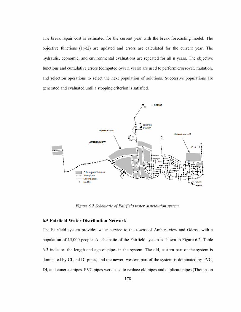
178
The break repair cost is estimated for the current year with the break forecasting model. The
objective functions (1)-(2) are updated and errors are calculated for the current year. The
hydraulic, economic, and environmental evaluations are repeated for all n years. The objective
functions and cumulative errors (computed over n years) are used to perform crossover, mutation,
and selection operations to select the next population of solutions. Successive populations are
generated and evaluated until a stopping criterion is satisfied.
Figure 6.2 Schematic of Fairfield water distribution system.
6.5 Fairfield Water Distribution Network
The Fairfield system provides water service to the towns of Amherstview and Odessa with a
population of 15,000 people. A schematic of the Fairfield system is shown in Figure 6.2. Table
6-3 indicates the length and age of pipes in the system. The old, eastern part of the system is
dominated by CI and DI pipes, and the newer, western part of the system is dominated by PVC,
DI, and concrete pipes. PVC pipes were used to replace old pipes and duplicate pipes (Thompson

179
2011). The unit price of PVC pipe obtained from a Canadian pipe distributor is indicated in Table
6-4. Pipe cleaning and cement-mortar lining costs from Walski (1986) in Table 6-4 were inflated
to 2010 dollars (start of planning period).
Table 6-3 Pipe material, length, and age in the Fairfield system.
Pipe Material Length (m)
Percent of Total
Length
Median Pipe Age
Concrete (C) 1,342 3.2 1993Cast Iron (CI) 10,959 26.4 1965Mortar Lined Ductile Iron (DI) 13,388 32.4 1985Polyvinyl Chloride (PVC) 15,774 38 1999Total 41,464 100 1985
Table 6-4 Unit costs of commercially-available PVC pipes and DI pipes cleaning and lining costs
(from Walski 1986).
Nominal Diameter of PVC Pipe
Inside Diameter of PVC Pipe
Unit Price of PVC Pipe
Pipe Cleaning and Lining Cost
(mm) (mm) ($/m) ($/m)150 160 29 63200 210 48 63250 258 72 68300 307 97 68350 356 103 68400 404 134 68450 453 169 N/A500 502 210 N/A600 600 304 N/A
The planning period in the Fairfield system spans the period 2010-2030. In the Year 2010, the
average day demand is 32 L/s in the Fairfield network. The average day demand is projected to

180
increase to 70.6 L/s in 2030 in Table 6-5 (CH2MHill 2007). A network expansion in the western
part of Fairfield (expansion area #1 in Figure 6.2) will be completed in Year 10. A second
expansion in the northern part of Fairfield will be completed in Year 20 (expansion area #2 in
Figure 6.2). Extended period simulation (EPS) and the diurnal pattern reported in Roshani et. al
(2012) were used to simulate average day demands over a typical 24-hour period in each year of
the planning period. Nodal pressures and pipe velocities were checked under maximum hour
demand conditions in Years 1, 10, and 20. Pressures and pipe velocities were checked under
maximum day demand + fire conditions at critical junctions J-514 and J-551 (Figure 6.2) in Years
1, 10, and 20. A needed fire flow of 33 L/s was adopted in accordance with Fire Underwriters
Survey (FUS) guidelines (FUS 1999). The hydraulic performance of the Fairfield system was
characterized with a total of 20 extended period simulations, 3 maximum hour demand
simulations, and 6 maximum day demand + fire flow simulations.
Table 6-5 Projected annual demand growth rates and current and projected water demands in
the Town of Amherstview (from CH2MHill 2007).
Water Use Land Use (%)Annual
Growth Rate (%)
2010 Present Water Demand
(L/s)
2030 Projected Water Demand
(L/s)
Residential 68 3.5 20 40Multi-residential 18 3.5 6 12Commercial 2 2 1 2Institutional 8 2 2 3.7Industrial 10 1 3 4.1New Industrial - - 0 8.8Total 100 32 70.6
181
To characterize energy use over the planning period (20 years), annual energy use was calculated
in each year by entering the average day diurnal pattern from Roshani et al. (2012) into
EPANET2 to simulate the pumping head and discharge over a 24-h period. Heads and discharges
were entered into the brake horsepower equation to calculate daily energy use and then multiplied
by 365 days to estimate annual energy use. This procedure was repeated for each year and the
total energy use over the 20-year planning period was calculated by summing annual energy use.
The annual energy use was multiplied by the average price of electricity of 8¢/kWh (OEB 2012)
to calculate the annual energy cost. The electricity price was assumed constant in the absence of
reliable electricity price forecasting data.
The mass of GHG emissions linked to pumping operations was calculated using projections of
Canada’s future energy fuel mix and GHG emission intensity factors (EIFs) produced by National
Energy Board (NEB 2007) and S & T Consultants Inc. (2008). The projected average emission
intensity factors for Canada were applied to the Eastern Ontario region since the Ontario and
average Canadian fuel mixes are similar (Environment Canada 2009). The full details of the
energy fuel mix and emission intensity factor analysis are presented in Roshani et al. (2012). The
GHG costs in (2) were calculated by multiplying the mass of GHG emissions in a particular year
by the appropriate carbon tax level for that year (Table 6-1). Note that the carbon tax values in
Table 6-1 for the years 2035 and 2040 were not used in the analysis since the planning period
spans the Years 2010-2030.
6.6 Results and Discussions
Six carbon mitigating scenarios were examined in this study. Scenario 1 (Scn. 1) is the “No Tax”
(NT) scenario where no carbon tax is levied and the discount rate stands at the current level of 8%
for public infrastructure projects in Canada (TBS 2007). In Scenario 2 (Scn. 2), no carbon tax is

182
levied and the discount rate is lowered to 1.4%, as suggested by Stern et al. (2006). In Scenario 3
(Scn. 3), the NRTEE “Slow and Shallow” (SS) carbon tax trajectory is applied and the discount
rate is set to 8%. In Scenario 4 (Scn. 4), the NRTEE “Slow and Shallow” (SS) carbon tax
trajectory is again applied and the discount rate is set to 1.4%. In Scenario 5 (Scn. 5), the NRTEE
“Fast and Deep” (FD) carbon tax trajectory is applied and the discount rate is set to 8%. In
Scenario 6 (Scn. 6), the NRTEE “Fast and Deep” (FD) carbon tax trajectory is applied and the
discount rate is set to 1.4%. In this study, capital costs, operating costs, and GHG costs are
discounted using the same constant discount rate.
6.6.1 Effect of Discount Rate and Carbon Tax on the Location of Pareto Fronts
The optimization algorithm was run for Scenarios 1 through 6 and the Pareto fronts generated in
each scenario are indicated in Figure 6.3. The discount rate applied in each scenario has a large
impact on the location of the Pareto fronts in Figure 6.3. Scenarios 1, 3, and 5 with a high
discount rate of 8% have Pareto fronts in the lower-left area of Figure 6.3. This is because a small
weight is placed on future capital and operational costs which reduces the cost components in the
objectives functions (1)-(2). Conversely, Scenarios 2, 4, and 6 with a low discount rate of 1.4%
have Pareto fronts in the upper-right area of Figure 6.3 since a greater weighting is placed on
future costs. The discount rate also has an impact on the shape (width and the height) of the
Pareto fronts. In Scenarios 2, 4, and 6 with a low discount rate of 1.4%, the width of the Pareto
fronts sits at approximately $3.0 M while in Scenarios 1, 3, and 5 (discount rate of 8%), the front
width sits at approximately $2 M. This is an artifice of compound discounting where a lower
discount rate tends to increase the sensitivity of present value costs to changes in future costs.

183
Figure 6.3 Pareto fronts generated in Scenarios 1 through 6.
The results in Figure 6.3 suggest that the carbon tax has a small impact on costs and the location
of Pareto fronts. When the discount rate is set to 8%, the FD carbon tax trajectory in Scenario 5
(Scn. 5) lowers the operational costs and the Pareto front of this scenario dominates all others.
This is owing to the fact that the higher carbon tax level place a higher weighting on electricity
costs tied to leakage and frictional energy losses in old deteriorated pipes which encourages the
search process to invest in early pipe rehabilitation to reduce subsequent energy requirements and
costs. When the discount rate is set to 1.4%, the impact of the FD carbon tax trajectory is much
less significant. This is evident in Figure 6.3 where the Pareto front of Scenario 6 (CT=FD,
DR=1.4%) overlaps almost perfectly with the Scenario 2 front (CT=NT, DR=1.4%). The lower
discount rate of 1.4% places a heavy weighting on future energy-related costs (leakage, frictional
184
losses) and thus encourages the search process to invest heavily and early in pipe rehabilitation
and replacement in both Scenarios 2 and 6. The weighting effect of the discount rate outstrips that
of the carbon tax and thus reduces the influence of the FD trajectory in forcing the search process
to adopt early replacement and rehabilitation. Interestingly, the Scenario 4 front (CT=SS,
DR=1.4%) is dominated by the Scenario 2 front (CT=NT, DR=1.4%) where no carbon tax is
applied. It is possible that in the SS trajectory of Scenario 4, the carbon tax is not increased fast
enough to place a large enough weight on future costs. As a result, the search process fails to
invest early in rehabilitation to decrease future costs in any significant way.
In the sections that follow, the energy use, GHG emissions, and costs will be compared between
solutions located at opposite ends of the Pareto fronts in Figure 6.3. In this figure, select solutions
in distinct regions of each Pareto front are indicated with a circle. These solutions are the
minimum capital cost solutions (left side of fronts), the minimum operational cost solutions (right
side of fronts), and the minimum total cost solutions (at or near the elbow of the fronts). In Table
6-6 through Table 6-8, the minimum capital cost solution is identified with the hyphenated
identifier “-1” (e.g., Scn. 1-1), the minimum operational cost solution is identified with “-2” (e.g.,
Scn. 1-2), and the minimum total cost solution is identified with “-3” (e.g., Scn. 1-3).
6.6.2 Effect of Discount Rate and Carbon Tax on Energy Use and GHGs
Discount rate was found to have a small influence on energy use and GHG emissions generated in
the Fairfield distribution network. At different carbon tax levels, lowering the discount rate from
8% to 1.4% was found to decrease GHGs from 0.3-7.6% in the minimum total cost solutions (“-
3”) of Table 6-6. (It is noted that lowering the discount rate from 8% to 1.4% under the SS carbon
tax trajectory resulted in a 0.9% increase in GHGs.) These results are explained by a lower
discount rate that places more weight on future costs and encourages the search process to invest
185
in rehabilitation in the opening years to lower the continuing costs linked to leakage and break
repairs that dominate (2). In the process of reducing lost water and repair costs, the search process
also reduces energy and GHG costs and emissions (albeit by smaller amounts) even though these
last two costs only account for a small portion of the operational cost in (2).
Applying a carbon tax on electricity was found to produce modest increases and decreases in
GHG emissions across minimum total cost solutions (“-3”) in Scenarios 1 through 6. At a
discount rate of 8% in Table 6-6, moving from a NT to a SS tax trajectory produced a 3.3%
increase in GHG emissions while moving from a SS to a FD trajectory produced a 1.3% increase
in GHG emissions. At a discount rate of 1.4%, moving from a NT to a SS trajectory resulted in a
slight increase of 4.6% in GHG emissions, while a move from a SS to a FD trajectory resulted in
a decrease of 9.6% GHG emissions. The small sensitivity of GHG emissions to an increase in
carbon tax is owing to the fact that the energy and GHG costs account for a small portion of the
annual operational cost (approximately 6~8%) relative to the lost water and repair costs in (2).
Most of the energy to pump water is used to satisfy the static head of 48 m in the system which is
unaffected by pipe rehabilitation.

186
Table 6-6 Average annual costs, annual greenhouse gas emissions, present value capital costs, present value operational costs, and present value
total costs for select solutions generated in Scenarios 1 through 6.
PV Opr.Cost
Break Leak Energy Cap. Cost Opr. Cost Total Cost GHG ($M)(5)
Scn. 1-1(1) 48.4 282.7 42.8 334.2 373.9 708.1 0 90.5 3.7 3.6 7.3Scn. 1-2(2) 18.1 110.8 39.4 491.8 168.2 660 0 83.9 5.5 2 7.5Scn. 1-3(3) 28.1 166 41.4 361.7 235.5 597.1 0 88 4 2.4 6.5Scn. 2-1 49 259.8 43.9 313.6 352.7 666.3 0 93.4 5.5 6.1 11.6Scn. 2-2 18.2 99.3 40.8 518.1 158.3 676.5 0 86.9 9 2.9 11.8Scn. 2-3 22.6 131.1 41.2 359.4 194.9 554.2 0 87.7 6.3 3.5 9.8Scn. 3-1 56.6 284 43.9 333.5 387.5 721 2.9 93 3.4 3.7 7.2Scn. 3-2 37.9 166.4 41.7 562.9 248.8 811.7 2.8 88.5 5.8 2.6 8.4Scn. 3-3 43.5 231.2 42.9 338.7 320.5 659.2 2.8 90.9 3.6 3.1 6.7Scn. 4-1 55.4 319.8 46.5 338.9 424.7 763.6 3.1 98.6 6 7.3 13.3Scn. 4-2 21.8 120.8 41.9 497.5 187.1 684.7 2.7 89.4 8.7 3.3 12Scn. 4-3 28.9 165.8 43.1 362.7 240.7 603.4 2.8 91.7 6.4 4.2 10.6Scn. 5-1 45.9 302.2 43.2 301 398.8 699.7 7.5 91.2 3.3 3.7 7Scn. 5-2 18.8 99.7 38.4 490.7 163.3 654.1 6.5 81.4 5.2 1.9 7.1Scn. 5-3 20 134.6 42.2 368.6 203.8 572.4 7 89.7 4.1 2.1 6.2Scn. 6-1 34.8 213.4 44.1 318.4 299.5 617.9 7.3 93.7 5.6 5.2 10.8Scn. 6-2 17.7 88.6 38.9 448.4 152 600.4 6.7 82.1 7.8 2.7 10.5Scn. 6-3 20.8 117.2 39.3 379.8 184.1 563.9 6.8 82.9 6.6 3.3 9.9
(3) The “-3” identifier denotes the minimum total cost solution.(4) NT: No Tax, SS: Slow and Shallow, FD: Fast and Deep.(5) Million dollars.
FD 1.4
(1) The “-1” identifier denotes the minimum capital cost solution.(2) The “-2” identifier denotes the minimum operational cost solution.
SS 1.4
FD 8
NT 1.4
SS 8
Annual GHG-e (tonne)
PV Cap. Cost ($M)
PV Total Cost ($M)
NT 8
Solution Tax Scn. (4) DR (%)Average Annual Cost ($1,000)

187
Table 6-7 Main length rehabilitated, age of rehabilitation, and percent of mains rehabilitated for select solutions in Scenarios 1 through 6.
DR(%)
Scn. 1(1) NT 8 47,397 31.3 66.1 10,914 30.1 15.2 13,438 29.9 18.7Scn. 2 NT 1.4 47,726 32.5 64.9 11,148 32 15.2 14,622 30.4 19.9Scn. 3 SS 8 43,577 30.9 64.6 12,078 32.3 17.9 11,824 28.2 17.5Scn. 4 SS 1.4 46,177 31.4 63 12,972 29.3 17.7 14,131 27.8 19.3Scn. 5 FD 8 46,261 31.4 64.6 10,686 29.4 14.9 14,700 29 20.5Scn. 6 FD 1.4 51,459 29.6 68.5 11,056 27.2 14.7 12,625 32.2 16.8
(1) The minimum total cost solution was selected for each scenario.(2) NT: No Tax, SS: Slow and Shallow, FD: Fast and Deep.
Percent of Total
Length (%) Length (m)
Avg. Age (Year)
Percent of Total
Length (%)Scenario
Pipe Replacement Pipe Duplication Lining
Tax Scn.(2) Length (m)Avg. Age
(Year)
Percent of Total
Length (%) Length (m)
Avg. Age (Year)

188
Table 6-8 The length and percent of mains rehabilitated over the planning period for select solutions in Scenarios 1 through 6.
1~6 7~13 14~20 1~6 7~13 14~20 1~6 7~13 14~20 1~6 7~13 14~20
Scn. 1(1) 71,749 19,672 (27) 6,812 (9) 20,913 (29) 4,672 (7) 2,191 (3) 4,052 (6) 5,612 (8) 2,199 (3) 5,626 (8) 29,956 (42) 11,202 (16) 30,591 (43)
Scn. 2 73,496 17,851 (24) 7,829 (11) 22,046 (30) 4,113 (6) 1,987 (3) 5,048 (7) 8,108 (11) 2,052 (3) 4,462 (6) 30,073 (41) 11,868 (16) 31,556 (43)
Scn. 3 67,479 19,710 (29) 5,934 (9) 17,933 (27) 1,325 (2) 2,899 (4) 7,854 (12) 5,670 (8) 975 (1) 5,179 (8) 26,704 (40) 9,809 (15) 30,966 (46)
Scn. 4 73,280 20,328 (28) 5,501 (8) 20,348 (28) 5,827 (8) 2,336 (3) 4,809 (7) 6,803 (9) 2,632 (4) 4,696 (6) 32,958 (45) 10,469 (14) 29,853 (41)
Scn. 5 71,648 18,751 (26) 7,778 (11) 19,732 (28) 4,902 (7) 1,130 (2) 4,655 (6) 9,019 (13) 1,391 (2) 4,290 (6) 32,672 (46) 10,299 (14) 28,677 (40)Scn. 6 75,140 21,559 (29) 9,621 (13) 20,279 (27) 3,320 (4) 2,527 (3) 5,209 (7) 6,630 (9) 2,073 (3) 3,922 (5) 31,509 (42) 14,221 (19) 29,411 (39)
(1) The minimum total cost solution was selected for each scenario.(2) The first number is the length of pipe rehabilitated and the number in parentheses is the percent of the total length of pipe rehabilitated.
Scenario Total Length (m)
The length and the percent of pipe rehabilitatedReplaced (m) (%)(2) Duplicated (m) (%) Relined (m) (%) Total (m) (%)

189
6.6.3 Effect of Discount Rate and Carbon Tax on Water Loss and Break Repair Cost
The results in Table 6-6 suggest that lowering the discount rate significantly reduces pipe break
repair costs and leakage costs across minimum total cost solutions (“-3”) in Scenarios 1 through
6. At different carbon tax levels, reducing the discount rate from 8% to 1.4% reduces the annual
break repair costs by 19.6-33.6%, and annual leakage costs by 12.9-28.3%. (It is noted that for the
FD trajectory, lowering the discount rate from 8% to 1.4% results in a 4% increase in annual
repair cost.) Lowering the discount rate places more weight on continuing leakage and pipe break
repair costs. This increased weighting in turn encourages the search process to find solutions that
invest heavily and early in pipe rehabilitation to reduce annual leakage and repair costs incurred
in the middle and end of the planning period.
Table 6-6 suggests that carbon tax can also have a significant impact on annual pipe break repair
cost and leakage cost across minimum total cost solutions (“-3”) in Scenarios 1 through 6.
Increasing the carbon tax from NT to SS significantly increased annual break repair cost by 27.9-
54.8% (for 1.4% and 8% rates) and annual leakage cost by 26.5-39.2% (for 1.4% and 8% rates).
This is because the SS tax trajectory produces only small GHG costs in the optimization and fails
to forcefully steer the search process to rehabilitate pipes early in the planning period.
Conversely, increasing the carbon tax further from SS to FD significantly decreased annual break
repair cost by 28.0-54.0% and leakage cost by 29.3-41.8% (for 1.4% and 8% rates). The FD tax
trajectory (unlike its SS counterpart) is aggressive enough to drive the search process to
rehabilitate pipe early in the planning period to significantly decrease pipe breaks and leakage in
the system.
6.6.4 Effect of Discount Rate and Carbon Tax on Rehabilitation Decision Type and Timing
The impact of discount rate on the length of pipe replaced, pipe lined, and pipe duplicated was
examined in Table 6-7. This table indicates the length, average age and percent of total length of

190
pipe replaced, pipe duplicated, and pipe relined for the minimum total cost solutions (“-3”) in
Scenarios 1 through 6. Table 6-7 indicates that lowering the discount rate from 8% to 1.4% at all
carbon tax levels leads to a modest 0.7-11.2% increase in pipe replacement length and a modest
2.1-7.4% increase in pipe duplication length. This is owing to a low discount rate that places a
higher weight on future operational costs and thus encourages the search process to increase the
length of pipes replaced and duplicated to lower costs linked to leakage and energy use. Further,
lowering the discount rate from 8% to 1.4% under the NT and SS tax trajectories increases the
length of lined pipe by 8.8-19.5%. However, lowering the discount rate from 8% to 1.4% under
the FD tax trajectory decreases the length of lined pipe by 14.1%. Here, the FD trajectory
imposes a higher weight on operational cost to encourage the search process to invest in pipe
replacement and pipe duplication and reduce the length of lined pipe.
The impact of carbon tax on the length of pipe replaced, pipe lined, and pipe duplicated for
minimum total cost solutions (“-3”) in Scenarios 1 through 6 was also examined in Table 6-7.
Moving from a NT to a SS trajectory (at 8% and 1.4% rates) produced a small 3.2%-8.0%
decrease in pipe replacement length, a modest 10.7%-16.4% increase in pipe duplication, and a
modest 3.4%-12.0% decrease in pipe lining. Here, the decrease in pipe replacement is
accompanied by an increase in pipe duplication to ensure an adequate level of hydraulic capacity
and contain frictional losses in the network. Further, moving from a SS to a FD trajectory (at 8%
and 1.4% rates) produced a modest 6.2%-11.4% increase in pipe replacement length, a modest
11.5-14.8% decrease in pipe duplication, and a significant 24.3% increase in lining (at an 8%
rate) and a modest 10.6% decrease in lining (at an 1.4% rate). Since the FD trajectory imposes a
large weight on future energy costs, it encourages the search process to select solutions which
rely heavily on pipe replacement and pipe duplication to reduce leakage and frictional losses –
two factors that affect energy use.

191
The impact of discount rate on the timing of pipe rehabilitation was also examined. Table 6-8
indicates the total length of pipe replaced, duplicated, and lined over three time intervals within
the 20-year planning period (e.g., Years 1-6, Years 7-13, and Years 14-20) for the minimum total
cost solutions (“-3”) in Scenarios 1 through 6. The results in Table 6-8 suggest that lowering
discount rate from 8% to 1.4% tends to shift the rehabilitation activities to the first and second
time intervals. This is because a low discount rate puts more weight on future operational costs
and thereby encourages the search process to choose solutions that shift pipe replacement,
duplication, and lining to the beginning and middle of the planning period to lower the present
value of these costs.
The results in Table 6-8 also suggest that moving to a more aggressive carbon tax trajectory (from
NT to FD) tends to shift rehabilitation activities to the first and second time intervals. The reason
again is that a higher carbon tax places more weight on future energy use which in turn
encourages the search process to seek out solutions that place their rehabilitation activities near
the beginning of planning period to minimize the present value of carbon tax-related costs. This is
corroborated by data in Table 6-7 that suggests that pipe age at the time of rehabilitation is lower
in scenarios with a low discount rate and a carbon tax trajectory.
6.6.5 Differences in Leakage Costs, Pipe Break Repair Costs, and Energy Costs across
Minimum Capital Cost Solutions and Minimum Operational Cost Solutions
The differences in leakage, pipe repair, and energy costs between the minimum capital cost
solutions and minimum operational cost solutions in Scenarios 1 through 6 was also examined.
The leakage cost was found to vary significantly between minimum capital cost solutions and
minimum operational cost solutions since it accounts for the largest portion of the operational
cost in the Fairfield system. The central and eastern parts of the Fairfield network are populated
with old CI and DI water mains with high leakage levels. The high leakage level presents an

192
opportunity for the search process to significantly reduce the costs of leakage by investing heavily
and early in pipe rehabilitation and replacement of old CI and DI pipes in these regions. Evidence
of this is found in Table 6-6 where for all 6 scenarios, the leakage cost for minimum operational
cost solutions (“-2”) is 41.4-67% lower than that of the minimum capital cost solutions (“-1”).
Further evidence is found in Figure 6.4 which compares the annual leakage cost between the
minimum capital cost solution of Scenario 6 (Scn. 6-1) and the minimum operational cost
solution of Scenario 6 (Scn. 6-2) (where the FD tax and a discount rate of 1.4% are applied). At
the beginning of the planning period, both solutions have approximately the same annual leakage
cost. However, the minimum operational cost solution benefits from heavy and early investment
in pipe rehabilitation which reduces the leakage through the end of the planning period.
Conversely, in the minimum capital cost solution, the search process instead chooses to reduce
pipe rehabilitation investments in the middle and near the end of the planning period which
increases leakage and operational cost in the middle years to the end of the planning period.
0
50
100
150
200
250
300
350
1 2 3 4 5 6 7 8 9 10 11 12 13 14 15 16 17 18 19 20Time (Year)
Scn. 6-1: Min. Capital Cost (CT= FD; DR=1.4%)Scn. 6-2: Min. Operational Cost (CT= FD; DR=1.4%)
Ann
ual L
eaka
ge C
osts
($1,
000)
Figure 6.4 Time variation of annual cost of lost water for minimum capital cost solution (“-1)
and minimum operational cost solution (“-2”) of Scenario 6 (CT=FD, DR=1.4%).

193
Similarly, the pipe break repair cost was found to vary significantly between minimum capital
cost solutions and minimum operational cost solutions. Table 6-6 shows that for all 6 scenarios,
the pipe break cost for minimum operational cost solutions (“-2”) was 33.0-62.8% lower than that
of the minimum capital cost solutions (“-1”). This is owing to the fact that in minimum
operational cost solutions (“-2”), there is a heavy and early investment in pipe replacement and
rehabilitation to lower continuing pipe repair costs.
The annual energy costs and annual GHG emissions of the minimum operational cost solutions
were also found to be lower than that of the minimum capital cost solutions. Table 6-6 indicates
that the annual energy costs of the minimum operational cost solutions (“-2”) were 5-11.8%
lower than that of the minimum capital cost solutions (“-1”). Similarly, the annual GHG
emissions of the minimum operational cost solutions (“-2”) were 4.8-12.4% lower than the
minimum capital cost solutions (“-1”). This is again owing to the fact that minimum operational
cost solutions (“-2”) benefit from heavy and early investment in pipe replacement and pipe
rehabilitation. Newly replaced pipes have more capacity (e.g., higher Hazen-Williams ‘C’
factors) and reduce the frictional losses and the energy required to pump water through them.
Newly replaced pipes also leak less which reduces the pumped volume and energy use and GHG
emissions linked to pumping water.
6.7 Sensitivity Analysis
The previous scenario analysis indicated that the main drivers of cost and GHG emissions were
water demand, leakage, and pipe breaks. A sensitivity analysis was performed to examine the
impact of selected parameters (forecasted demand, initial leak rate, leak growth rate, initial break
rate, break growth rate, and Hazen-Williams ‘C’ factor) on the objective function cost values and
on GHG emissions. All sensitivity analysis runs were performed for Scenario 6 where a FD tax

194
trajectory and a discount rate of 1.4% were applied. A total of 8 sensitivity analysis runs were
performed to examine: (1) a 15% increase in forecasted water demand, (2) a 15% decrease in
forecasted water demand, (3) a 15% increase in initial leak rate, (4) a 15% decrease in initial leak
rate, (5) a 15% increase in leak growth rate, (6) a 15% increase in initial break rate, (7) a 15%
increase in break growth rate, and (8) a 15% decrease in Hazen-Williams ‘C’ factor as indicated
in Table 6-9. The mean and standard deviations of costs were computed with the objective
function values (and their cost components) for all the solutions on the Pareto front of the final
generation.
6.7.1 Capital Costs
The results in Table 6-9 suggest that capital costs are moderately sensitive to uncertainties in
forecasted demand and leakage growth. Table 6-9 indicates that a 15% increase in forecasted
demand results in a 10.3% increase in the present value of capital cost. A 15% increase in
forecasted demand results in a 9% increase in pipe replacement cost and a 19% increase in pipe
duplication cost. These results suggest that an increase in demand encourages the search process
to replace and duplicate pipes to increase the hydraulic capacity of the network. Further, a 15%
decrease in forecasted water demand results in a 7.6% decrease in pipe replacement cost. Since
pipe replacement accounts for a large portion of capital costs, a decrease in pipe replacement
creates savings to undertake a 12.6% increase in pipe lining and an additional 28.3% increase in
pipe duplication expenditures.
Similarly, a 15% increase in leakage growth results in a 10.3% increase in the present value of
capital cost. The same increase in leakage growth rate results in a 5% increase in pipe
replacement cost, a 35% increase in pipe duplication cost, and a 4% increase in pipe lining cost.
To offset the higher leakage level, the search process replaces, lines, and duplicates old,

195
deteriorated pipes. Pipe duplication reduces pressures in the network and thereby decreases
leakage. (It should be noted that part of this pipe duplication is to increase the system capacity to
supply the lost water in the network).
6.7.2 Operational Costs
The results in Table 6-9 suggest that operational costs are moderately sensitive to uncertainties in
forecasted demand and highly sensitive to leakage growth. Table 6-9 indicates that a 15%
increase in forecasted demand results in a 21.4% increase in the present value of operational cost
and that a 15% increase in leakage growth results in a 85.7% increase in the present value of
operational cost. Not surprisingly, increases in forecasted water demand and leak growth rate
produce corresponding increases in annual energy costs and annual lost water costs (see Table
6-9). Increasing the leakage growth rate by 15% also leads to a reduction of 21.2% in annual
break repair cost. This is owing to a higher leak rate that drives the search process to choose
solutions with more pipe replacement and pipe duplication which also reduces the number of pipe
breaks in the system.

196
Table 6-9 Results of the sensitivity analysis.
-15%
Hazen-Williams ‘C’
6.8 (0.8) 7.5 (1.0) 6.8 (1.1) 7.0 (0.94) 6.9 (0.8) 7.5 (0.8) 6.9 (0.8) 6.8 (0.9) 6.7 (0.9)Average Annual Pipe Replacement Cost ($1,000) 252.6 (41.3) 275.3 (44.4) 233.3 (45.5) 252.8 (43.2) 243.2 (41.2) 264.7 (38.0) 243.3 (36.9) 251.6 (37.3) 242.8 (45.2)
Average Annual Lining Cost ($1,000) 45.2 (6.2) 42.6 (6.1) 50.9 (8.7) 46.1 (7.2) 46.0 (6.9) 47.0 (6.9) 50.3 (7.3) 46.6 (7.1) 48.6 (7.7)
Average Annual Pipe Duplication Cost ($1,000) 61.9 (9.5) 73.7 (13.6) 79.4 (15.3) 65.8 (12.5) 74.2 (10.9) 83.5 (13.0) 71.8 (11.5) 63.2 (14.4) 67.1 (11.6)
Average Annual New Pipe Installation Cost ($1,000) 27.3 (3.4) 34.1 (3.7) 25.1 (3.3) 34.5 (5.4) 27.3 (4.0) 31.5 (3.3) 27.3 (4.6) 28.4 (4.4) 26.1 (3.8)
4.2 (1.0) 5.1 (1.3) 5.0 (1.5) 4.9 (1.4) 4.1 (1.0) 7.8 (1.8) 4.5 (1.0) 4.9 (0.9) 4.5 (1.2)Average Annual Lost Water Cost ($1,000) 160.1 (50.8) 196.0 (63.7) 199.4 (74.5) 201.3 (69.3) 154.0 (46.6) 366.5 (102.7) 172.4 (50.8) 159.9 (37.0) 176.3 (59.0)
Average Annual Energy Cost ($1,000) 41.2 (1.9) 49.6 (2) 41.7 (2.3) 42.8 (1.9) 42.1 (1.5) 47.7 (2.4) 41.9 (1.5) 41.7 (1.3) 41.9 (1.4)Average Annual Break Repair Cost ($1,000) 29.7 (9.4) 36.1 (11.4) 36.3 (12.8) 31.1 (9.7) 31.3 (9.2) 23.4 (5.4) 35.3 (10.4) 69.8 (18.4) 31.8 (9.7)
Average Annual GHG Cost ($1,000) 6.9 (0.3) 8.1 (0.4) 6.7 (0.4) 7.1 (0.3) 7.0 (0.2) 7.5 (0.4) 7.0 (0.2) 7.0 (0.2) 7.0 (0.2)
Average Annual GHG Emissions (tonnes) 87.5 (4.2) 105.8 (4.1) 89.3 (5) 91.1 (4.2) 89.5 (3.2) 102.5 (5.0) 89.2 (3.4) 88.8 (2.9) 89.2 (3.1)
Capital Cost ($M)(1)
Operational Cost ($M)
(1) Million dollars.(2) The first number is the mean value and the second number is the standard deviation.
Parameters Scn.6 (CT=FD;
DR=1.4%)
Scenario
+15% Future
Demand-15% Future
Demand+15% Initial
Leak-15% Initial
Leak
+15% Leak Growth
Rate+15% Initial
Break
+15% Break Growth
Rate

197
6.7.3 Greenhouse Gas Emissions
The results in Table 6-9 suggest that GHG emissions are moderately sensitive to water demand
and leakage growth rate. Specifically, a 15% increase in forecasted water demand results in a
20.9% increase in annual GHG emissions and a 15% increase in leak growth rate results in a
17.1% increase in annual GHG emissions. Not surprisingly, an increase in water demand and
leakage both increase the pumping and electricity requirements of the system and the GHGs
associated with electricity production to operate the pumps.
6.8 Summary and Conclusions
A new multi-objective optimization approach was developed and used to solve the optimal pipe
rehabilitation timing problem for six carbon mitigating scenarios. The optimization approach was
applied to the real-world Fairfield water distribution network in eastern Ontario, Canada. The
results suggested that adopting a low discount rate and levying a carbon tax had a small impact in
reducing energy use and GHG emissions because these accounted for a small portion of the total
operational costs. Further, a low discount rate and the application of a carbon tax had a significant
impact in reducing leakage and pipe breaks and encouraged the search process to invest in
rehabilitation early in the planning period to reduce the continuing costs of leakage, pipe repair,
energy and GHG emissions. A sensitivity analysis suggested that water demand and leakage
growth rate had a moderate to significant impact on the present value of capital and operational
costs and on GHG emissions in the Fairfield system.
6.9 Acknowledgements
The authors thank David Thompson, P.Eng., at Loyalist Township for providing data and advice
in the development of this paper. This research was financially supported by Queen’s University
and the Natural Sciences and Engineering Research Council.

198
6.10 References
Ainger, C., Butler, D., Caffor, I., Crawford-Brown, D., Helm, D., Stephenson, T. (2009). “A Low
Carbon Water Industry in 2050.” UK Environment Agency, Bristol, UK,
<http://cdn.environment-agency.gov.uk/scho1209brob-e-e.pdf, Accessed: Oct. 25, 2012>.
Alvisi S., Franchini M. (2009). “Multiobjective Optimization of Rehabilitation and Leakage
Detection Scheduling in Water Distribution Systems.” Journal of Water Resources
Planning and Management, 135(6), 426-439.
Arai, N. (2012). “Best Practice: Water Leakage Prevention Controls”,
<www.nyc.gov/globalpartners/innovationexchange, Accessed: Oct. 1, 2012>.
Arulraj, G.P., and Suresh, H.R. (1995). “Concept Of Significance Index For Maintenance And
Design Of Pipe Networks.” Journal of Hydraulic Engineering, 121 (11), 833–837.
American Society of Civil Engineers (2009). “America’s Infrastructure Report Card: Drinking
Water.” <http://www.infrastructurereportcard.org/fact-sheet/drinking-water, Accessed:
Oct. 1, 2012>.
Brothers, K.J. (2001). “Water Leakage And Sustainable Supply-Truth Or Consequences?”
Journal of American Water Works Association, 93(4), 150-152.
Canadian Infrastructure Report Card (2012). “Volume 1: 2012 Municipal Roads and Water
Systems.” www.canadainfrastructure.ca, Accessed: Oct. 25, 2012> .
CH2MHill (2007). Fairfield Water Storage Project: Final Report. CH2M Hill, Ottawa, Ontario,
Canada.

199
Dandy, G.C., Engelhardt, M. (2001). “Optimal Scheduling Of Water Pipe Replacement Using
Genetic Algorithms.” Journal of Water Resources Planning and Management, 127(4), 214-
223.
Dandy, G.C., Engelhardt, M. (2006). “Multi-Objective Trade-Offs Between Cost And Reliability
In The Replacement Of Water Mains.” Journal of Water Resources Planning and
Management, 132 (2), 79-88.
Dandy, G., Roberts, A, Hewitson, C., and Chrystie, P. (2006). “Sustainability Objectives For The
Optimization Of Water Distribution Networks.” 8th Annual Water Distribution Systems
Analysis Symposium, Cincinnati, Ohio, 1-11.
Dandy, G., Bogdanowicz, A., Craven, J., Maywald, A., Liu, P. (2008). “Optimizing the
Sustainability of Water Distribution Systems.” 10th Water Distribution Systems Analysis
Symposium, Kruger National Park, South Africa, 267-277.
Deb, K., Pratap, A., Agarwal, S., Meyarivan, T. (2002). “A Fast And Elitist Multiobjective
Genetic Algorithm: NSGA-II.” IEEE Transactions on Evolutionary Computation, 6(2),
182-197.
Environment Canada. (2009). National Inventory Report: Greenhouse Gas Sources And Sinks In
Canada, Library and Archives Canada Cataloguing in Publication, Gatineau, Quebec.
European Environment Agency (2010). “Indicator Fact Sheet, WQ06, Water Use Efficiency (In
Cites): Leakage”, <http://www.eea.europa.eu/data-and-maps/indicators/water-use-
efficiency-in-cities-leakage/water-use-efficiency-in-cities-leakage, Accessed: Oct. 1,
2012>.

200
Fearnside, P.M., (2002). “Time Preference In Global Warming Calculations: A Proposal For A
Unified Index.” Ecological Economics, 41(1), 21-31.
Filion, Y.R., MacLean, H., Karney, B.W. (2004). “Life-Cycle Energy Analysis Of A Water
Distribution System.” Journal of Infrastructure Systems, 10(3), 120-130.
Fire Underwriters Survey (FUS) (1999). Water Supply for Public Protection. CGI Group Inc.,
Markham, Ontario, Canada.
Germanopoulos, G. (1985). “A Technical Note On The Inclusion Of Pressure Dependent Demand
And Leakage Terms In Water Supply Network Models.” Civil Engineering System, 2, 171-
179.
Goldstein, R., Smith, W. (2002). “Water and Sustainability: US Electricity Consumption for
Water Supply and Treatment: The Next Half Century.” Electric Power Research Institute,
<https://www.rivernetwork.org/rn/climate/EPRIwsv4, Accessed: Oct. 1, 2012>.
Hasselmann, K., Hasselmann, S., Giering, R., Ocana, V., and Storch, H.V. (1997). “Sensitivity
Study Of Optimal Co2 Emission Paths Using A Simplified Structural Integrated
Assessment Model (SIAM).” Climate Change, 37(2), 345–386.
Kleiner, Y., and Rajani, B. (1999). “Using Limited Data To Assess Future Needs.” Journal of
American Water Works Association, 91(7), 47-61.
Martinez, F., Conejos, P., and Vercher, J. (1999). “Developing An Integrated Model For Water
Distribution Systems Considering Both Distributed Leakage And Pressure-Dependent
Demands.” 26th ASCE Water Resources Planning and Management Division, ASCE,
Tempe, Arizona. 1-14.

201
Mailhot A, Poulin, A., Villeneuve, J.P. (2003). “Optimal Replacement Of Water Pipes.” Water
Resources Research, 39(5), 1136-1150.
National Energy Board (NEB). (2007). Canada’s Energy Future Reference Case and Scenarios to
2030: An Energy Market Assessment. National Energy Board Publications, Calgary,
Canada.
National Round Table on the Environment and the Economy (NRTEE). (2009). Achieving 2050:
A carbon pricing policy for Canada. Library and Archives Canada Cataloguing in
Publication, Ottawa, Ontario, Canada.
Ontario Energy Board (OEB). (2012). Regulated Price Plan Price Report. Queen’s Printer for
Ontario, Toronto, Ontario, Canada.
Roshani, E., Filion, Y.R. (2009). “Accounting for Greenhouse Gas Emissions in the Multi-
Objective Optimization of the Kamalsaleh Water Transmission Systems Using NSGA-II.”
Computing and Control in the Water Industry, Sheffield, UK. 799-805.
Roshani, E., MacLeod, S.P., Filion, Y.R. (2012). “Evaluating the Impact of Climate Change
Mitigation Strategies on the Optimal Design and Expansion of the Fairfield, Ontario Water
Network: A Canadian Case Study.” Journal of Water Resources Planning and
Management, ASCE, 138(2), 100-110.
Roshani, E., Filion, Y.R. (2012). “Event Based Network Rehabilitation Planning And Asset
Management.” 14th annual Water Distribution Systems Analysis Symposium, Adelaide,
Australia, 933-943.
Rossman, L.A. (2000). EPANET2 User’s Manual. US EPA, Washington, D.C.

202
Shamir, U., Howard, C.D.D. (1979). “An Analytic Approach To Scheduling Pipe Replacement.”
Journal of American Water Works Association, 71(5), 248–258.
Sharp, W., Walski, T.M. (1988). “Predicting Internal Roughness In Water Mains.” Journal of
American Water Works Association, 80(11), 34-40.
Stern, N., Peters, S., Bakhshi, V., Bowen, A., Cameron, C., Catovsky, S., Crane, D., Cruickshank,
S., Dietz, S., Edmonson, N., Garbett, S., L., Hamid, L., Hoffman, G., Ingram, D., Jones, B.,
Patmore, N., Radcliffe, H., Sathiyarajah, R., Stock, M., Taylor, C., Vernon, T., Wanjie, H.,
and Zenghelis, D. (2006). Stern Review: The Economics Of Climate Change. HM
Treasury, London, UK.
S & T Consultants Inc. (2008). 2008 GHGenius update, Natural Resources Canada, Ottawa.
Thompson, D. (2011) Personal Communication. Director of Engineering, Loyalist Township,
Ontario, Canada.
Treasury Board of Canada Secretariat (TBS) (2007). Benefit-Cost Analysis Guide Interim Report.
Treasury Board of Canada Secretariat, Ottawa, Ontario, Canada.
Walski, T.M., Pelliccia, A. (1982). “Economic Analysis Of Water Main Breaks.” Journal of
American Water Works Association, 74(3) 140-147.
Walski, T.M. (1986). “Predicting Costs Of Pipe Cleaning And Lining Projects.” Journal of
Transportation Engineering, 112(3), 317-327.
Wu, W., Simpson, A.R., Maier, H.R. (2008). “Multi-Objective Genetic Algorithm Optimization
Of Water Distribution Systems Accounting For Sustainability.” 10th Annual Symposium on
Water Distribution Systems Analysis, South Africa, 1-12.

203
Wu, W., Simpson, A.R., and Maier, H.R. (2010). “Accounting for Greenhouse Gas Emissions in
Multi-Objective Genetic Algorithm Optimization of Water Distribution Systems” Journal
of Water Resources Planning and Management, 136(2), 146-155.

204
Chapter 7
Conclusions
Climate change has been identified as a serious threat to human and economic security (Erwin et
al. 2012). The developed world has begun to address climate change by means of policy measures
such as carbon pricing (a carbon tax or cap-and-trade system) and economic discounting in
project planning. Since the water industry is a major user of fossil-based electricity, policies such
as a carbon tax and low discount rates can potentially stand to change the way water distribution
systems are designed, operated, and rehabilitated. The research in this thesis has sought to
examine the impact of climate change mitigation scenarios in the optimal WDS design/expansion,
operation, and rehabilitation planning of water distribution networks.
7.1 Overall Research Contributions
The overall contributions of this research are listed below. The first 6 research contributions
relate to the development of the single- and multi-objective optimization algorithms that account
for GHG emissions in the solution of the design/expansion, operation, and rehabilitation planning
problems. The remaining 2 research contributions relate to the new scenario analyses that were
performed to examine the impact of climate change mitigation scenarios on energy use, GHG
emissions, and design/expansion, operation, and rehabilitation decisions in the optimization of
water distribution networks

205
7.1.1 Model Development
Contribution 1: The first research contribution is the development of the single- and multi-
objective optimization algorithms that account for GHG emissions in the solution of the water
distribution network design/expansion, operation and rehabilitation planning problems.
Contribution 2: The second contribution is the development of a new gene-coding scheme to
reduce the computational requirements to solve the optimal water distribution network operation
and rehabilitation planning problems. The proposed event-based method (Chapters 5 and 6)
reduces the length of each chromosome by 20 percent when compared to traditional approaches.
The gene-coding scheme is an important contribution because it makes it feasible to solve the
operation and rehabilitation optimization problems for large, complex networks.
Contribution 3: The third research contribution is the development of a new pump scheduling
optimization approach that can model a Programmable Logic Controller (PLC) system that
controls the real-time operation of pumps and reservoirs in a complex water transmission system
(Chapter 3).
Contribution 4: The fourth research contribution is the inclusion of a pipe break forecasting
model, a leakage forecasting model, and pipe wall roughness growth model in the water main
rehabilitation optimization algorithms of Chapters 5 and 6. This is the first water main
rehabilitation optimization model to include all three model types.
Contribution 5: The water distribution network rehabilitation algorithms of Chapters 5 and 6 are
the first to consider the full range of water main rehabilitation decisions such as pipe duplication,
pipe replacement, pipe lining, and new pipe installation.
Contribution 6: The sixth research contribution is the development of the graphical user
interface (GUI) used for all the algorithms presented in this thesis. The GUI was designed to

206
facility the entry and management of the extensive data involved in the simulation and
optimization of water distribution networks. The GUI was also designed to allow users without
any programming knowledge to use with ease.
7.1.2 Scenario Analyses
Contribution 7: The optimization algorithms developed in this research were applied to two
complex, real-world water systems. Previous research by Wu et al. (2010a, 2010b, 2012)
examined GHG emissions in small, hypothetical systems. The consideration of real, complex
systems in this research means that it could potentially contribute to the future evolution of
climate change mitigation policies as they pertain to the Canadian water industry.
Contribution 8: The scenario analyses presented in the case studies considered the full range of
demand conditions, including a 24-hour average day diurnal pattern, maximum hour demands,
maximum day demands, and fire flow. Previous research by Wu et al. (2010a, 2010b, 2012) only
considered the average day demand condition in its examination of GHG emissions in networks.
7.1.3 Research Findings in Case Studies
Chapter 3: The impacts of carbon mitigation scenarios on energy use and GHG emissions in
Kamalsaleh water transmission system were investigated. The results for single-objective
simulations indicated that carbon tax and discount rate have noticeable impact on the level of
reservoir storages in the case study while it produces a small reduction in the GHG emission. The
multi objective results indicated that the Pareto front shape (steepness) is affected by the discount
rate and carbon tax where modest investment in the capital cost produces significant reduction in
the operational costs. It should be noted that the results is only pertain to the KamalSaleh
transmission system and more research is needed to examine the effectiveness of discount rate
and carbon tax in reducing energy use and greenhouse gas emissions in low-lift transmission

207
system with different topographies, a range of water demand levels and diurnal patterns, a range
of pipeline diameters, and a range of reservoir configurations.
Chapter 4 investigated the effect of proposed Canadian climate change mitigation policies on the
energy use and GHG emissions in design and expansion of Fairfield water distribution system.
Results indicated that the proposed discount rates and GHG taxes have no significant impact on
the GHG emission. And the Fairfield WDS was not able to meet GHG reduction target set by the
Canadian government. Time declining emission intensity factor, relatively short design period of
the case study, and adequate hydraulic capacity in the Fairfield system to meet present and future
demands were the major contributors to the insensitivity of GHG emission and energy use to the
proposed policies. It worth mentioning that the results are limited to the Fairfield case study and
more investigation is necessary to determine the effectiveness of the proposed polices in other
networks in Canada.
Chapter 5 proposed the new event-based approach to find the optimal WDS rehabilitation
planning in Fairfield network. It examined the effect of asset management strategies such as
discounting and budget management on the capital and operational cost of rehabilitation
solutions. The results suggested that applying a budget constraint prohibited the search process
from investing early and heavily in pipe rehabilitation with a resulting increase in cost linked to
pipe leakage, pipe breaks, and energy use. Moreover, a sensitivity analysis showed that water
demand, leakage and break growth rates can have a moderate to significant impact on capital and
operational costs. The results are limited to Fairfield WSD and more investigations are necessary
to understand the impact of asset management strategies on the distribution of the water main
rehabilitation decisions especially when other network components such as pumps and tanks are
included in the search space.

208
Chapter 6 for the first time studied the effects of proposed carbon mitigation policies on optimal
rehabilitation planning of a WDS. The proposed model was applied to Fairfield network and
results indicated that low discount rate and high carbon tax have small impact of GHG reduction
while significantly decrease the leakage and pipe breaks. Further low discount rate and high
carbon tax encouraged the optimization engine to invest early in the planning period to reduce
leakage, energy, GHG costs, and pipe breaks. The results are limited to Fairfield WDS; additional
research could shed light on the effect of the carbon mitigation policies on the rehabilitation
options while renewing pump stations and tanks are considered.
7.2 Research Limitations
The embodied energy and GHG emissions linked to the material extraction, material production,
and manufacturing of water main materials such as PVC was not included in the optimization
algorithms for lack of data in Canada.
Only decision variables that pertain to water mains were optimized in the network
design/expansion and rehabilitation planning models of Chapters 4, 5, and 6. Other system
components such as pumps and elevated tanks were not optimized in these models. This is
justified on the grounds that water main assets often account for the largest asset value in many
networks. Further, no additional pumping station and elevated tank facilities were required in the
Fairfield water distribution network to meet forecasted future demands (Thompson 2011).
Given the large search space in the network design/expansion, operation, and rehabilitation
planning problems of Chapters 3, 4, 5, and 6, a stopping criterion based on a defined number of
generations was imposed on the optimized solutions. The implication is that the solutions
generated in the single-objective optimization are near-optimal solutions. Similarly, the Pareto-

209
optimal solutions generated in the multi-objective optimization are near optimal Pareto front.
There is still no universally accepted stopping criterion for heuristic search algorithms.
There are number of variables at play in the solution of the network design/expansion, operation,
and rehabilitation planning problems whose uncertainty was not characterized in the scenario and
sensitivity analyses of this thesis. Uncertain financial parameters such as electricity price, water
price, and budget limit were not considered in the analyses. Water demand and hydraulic
parameters such as peak demand factors and minimum and maximum pressure were not
considered in the analyses. Simulation variables such as expected service life of water main, and
lag times between rehabilitation events were not considered in the analyses. Genetic algorithm
optimization parameters such as population size, mutation and crossover probabilities, number of
evaluations were not considered in the analyses.
7.3 Recommendation for Future Work
Based on the research limitations highlighted above, future research should focus on making
advancements in the following areas:
Area 1: Future work could consider embodied energy use and GHG emissions associated with
material extraction, material production, and the manufacturing of system components such as
water mains (of different materials), pumps, elevated tanks, and reservoirs. Considering
embodied energy use and GHG emissions would help municipalities and water utilities better
understand the trade-offs in energy use and GHG emissions linked to capital infrastructure
investments and pumping water in a system over a specified planning horizon.
Area 2: Future work could consider an additional number of decisions variables to optimize such
as the sizing and sitting of pumps, elevated tanks, and reservoirs. While this would further
increase computational expense, it would allow municipalities and water utilities to better

210
understand the effects of making major capital investments in new pumping station and tank
facilities on the energy use and GHG emissions generate by their systems..
Area 3: Future work should also provide general recommendations on the practical number of
optimization generations required to find near-optimal solutions in the network design/expansion,
operation, and rehabilitation planning problems.
Area 4: Future work could focus on performing more comprehensive sensitivity analyses to
examine the impact of uncertain financial, pipe aging, water demand, hydraulic, and other
variables on the system costs, energy use, and GHG emissions of networks.
Area 5: There is a need to apply the optimization models developed in this thesis to other real-
world water distribution networks to better establish the relationship between key system
properties (e.g., topography, age of water main assets, etc.) and energy use and GHG emissions in
other complex, real-world systems. This knowledge is necessary to develop best practices that
municipalities and water utilities can use to guide their capital infrastructure budget planning and
achieve tangible reductions in operating and other systems costs and energy use.
7.4 References
Erwin S. I., Magnuson S., Parsons D., Tadjdeh Y., (2012) “Top Five Threats to National Security
in the Coming Decade”, National Defense Magazine, Nov 2012, Accessed Date Feb 2,
2013
<http://www.nationaldefensemagazine.org/archive/2012/November/Pages/TopFiveThreats
toNationalSecurityintheComingDecade.aspx>
Thompson, D. (2011) Personal Communication. Director of Engineering, Loyalist Township,
Ontario, Canada.

211
Wu, W., Simpson, A. R., and Maier, H. R. (2012) “Incorporation Of Variable-Speed Pumping In
Multiobjective Genetic Algorithm Optimization Of The Design Of Water Transmission
Systems.” Journal of Water Resources Planning and Management, Vol. 138, (5), 543-552.
Wu, W., Simpson, A. R., and Maier, H. R. (2010a). "Accounting for Greenhouse Gas Emissions
in Multiobjective Genetic Algorithm Optimization of Water Distribution Systems." Journal
of Water Resources Planning and Management, 136(2), 146-155.
Wu, W., Maier, H. R., and Simpson, A. R. (2010b). "Single-Objective versus Multi-Objective
Optimization of Water Distribution Systems Accounting for Greenhouse Gas Emissions by
Carbon Pricing." Journal of Water Resources Planning and Management, 136(5), 555-565.

212
Appendix A
OptiNET Validation Results
Summery of test functions
All of the optimization benchmark problems that have been used to validate the OptiNET are
listed in the following two tables. The first table contains the benchmarks without constraint and
the second table includes the benchmarks with constraints.
Table A- 1 Benchmarks without constraint used to validate OptiNET
SCH: Schaffer J. D., (1987) “Multiple Objective Optimization With Vector Evaluated Genetic Algorithms” in Proceedings of the First International Conference on Genetic Algorithms, J. J. Grefensttete, Ed. Hillsdale, NJ: Lawrence Erlbaum, 1987, pp. 93–100.
FON: Fonseca C. M., Fleming P. J., (1998) “Multiobjective Optimization And Multiple Constraint Handling With Evolutionary Algorithms—Part II: Application example,” IEEE Trans. Syst., Man, Cybern. A, vol. 28, pp. 38-47.
ZDT: Zitzler E., Deb K., Thiele L., (2000) “Comparison Of Multiobjective Evolutionary Algorithms: Empirical Results” Evol. Comput., vol. 8, no. 2, pp. 173-195.

213
Table A- 2 Benchmarks with constraints used to validate OptiNET
CONSTR: Deb, K., Pratap, A., Agarwal, S., Meyarivan, T. (2002). “A Fast And Elitist Multiobjective Genetic Algorithm: NSGA-II.” IEEE Transactions on Evolutionary Computation, 6(2), 182-197.
SRN: Srinivas N., Deb K., (1995) “Multiobjective Function Optimization Using Nondominated Sorting Genetic Algorithms,” Evol. Comput., vol. 2, no. 3, pp. 221-248.
TNK: Tanaka M., (1995) “Ga-Based Decision Support System For Multicriteria Optimization” in Proc. IEEE Int. Conf. Systems, Man and Cybernetics-2, pp. 1556-1561.
OptiNET test results vs. NSGA-II
0
1
2
3
4
0 1 2 3 4
Objective 1
Obj
ectiv
e 2
OptiNET
NSGA-II by Deb
Figure A- 1 Non-dominated Pareto front obtained on SCH benchmark

214
0
0.2
0.4
0.6
0.8
1
0 0.2 0.4 0.6 0.8 1
Objective 1
Obj
ectiv
e 2
OptiNET
NSGA-II by Deb
Figure A- 2 Non-dominated Pareto front obtained on FON benchmark
0
0.2
0.4
0.6
0.8
1
0 0.2 0.4 0.6 0.8 1
Objective 1
Obj
ectiv
e 2
OptiNET
NSGA-II by Deb
Figure A- 3 Non-dominated Pareto front obtained on ZDT1 benchmark

215
0
0.2
0.4
0.6
0.8
1
0 0.2 0.4 0.6 0.8 1
Objective 1
Obj
ectiv
e 2
OptiNET
NSGA-II by Deb
Figure A- 4 Non-dominated Pareto front obtained on ZDT2 benchmark
-1
-0.8
-0.6
-0.4
-0.2
0
0.2
0.4
0.6
0.8
1
0 0.1 0.2 0.3 0.4 0.5 0.6 0.7 0.8 0.9
Objective 1
Obj
ectiv
e 2
NSGA-II by Deb
OptiNET
Figure A- 5 Non-dominated Pareto front obtained on ZDT3 benchmark

216
0
1
2
3
4
5
6
7
8
9
10
0 0.2 0.4 0.6 0.8 1 1.2
Objective 1
Obj
ectiv
e 2
OptiNET
NSGA-II by Deb
Figure A- 6 Non-dominated Pareto front obtained on Constr benchmark
-250
-200
-150
-100
-50
00 50 100 150 200 250
Objective 1
Obj
ectiv
e 2
OptiNET
NSGA-II by Deb
Figure A- 7 Non-dominated Pareto front obtained on SRN benchmark

217
0
0.2
0.4
0.6
0.8
1
1.2
0 0.2 0.4 0.6 0.8 1 1.2
Objective 1
Obj
ectiv
e 2
OptiNET
NSGA-II by Deb
Figure A- 8 Non-dominated Pareto front obtained on TNK benchmark

218
Appendix B
Parallel Processing
Abstract
A high level of computational power is often needed to solve real-world engineering problems.
The introduction of multi-core Central Processing Units (CPUs) opened a new window for small
companies and academic researchers to benefit from high performance computing. OptiNET
benefits from two different parallel processing libraries, the Message Passing Interface (MPI) and
Task Parallel Library (TPL). In this appendix both of these libraries are applied to find the
optimal rehabilitation plane for a Fairfield water distribution system. The time required to
evaluate all solutions in the last generation were measured for increasing number of cores in both
approaches and compared.
Introduction
The introduction of multi-core Central Processing Units (CPUs) in 2005 revolutionized the
software industry. Since then the demand for multi-core computing has increased and it has
become progressively less expensive. For example, one can now purchase a desktop computer
with 24 cores for less than $3,000. Suddenly, parallel computing has become available to a much
broader range of users, including consulting engineers, through new programming interfaces and
toolboxes.
Increasingly, engineers are turning to optimization to plan the design, expansion, and
rehabilitation of water distribution systems. High computational power is required to find the
optimal solution in real networks which tend to have a large number of pipes and components and
thus impose long run times on a network solver to evaluate the hydraulic and/or water quality
conditions. Optimization is one of the best examples of algorithms in which tasks could be run in

219
parallel. In fact, optimization algorithms are known as “attractively” parallel algorithms
(Microsoft Corporation 2008). Since these algorithms are computationally-intensive, they are best
solved on multi-cores computers or a cluster machine (Microsoft Corporation 2008).
There are several parallel programming interfaces available in the market and most of them are
open source. The objective of this paper is to present the parallelization of code to solve the
multi-objective optimization of a real-world water distribution network in Amherstview, Ontario,
Canada. Two well-known open source interfaces, TPL and MPI.net, were used to solve the multi-
objective problem, with significant increases in computational speed. Both methods will be
introduced and discussed in the paper, and the pseudo-code implementation used to parallelize the
optimization algorithm will be discussed.
Methodology/Process
Parallel Processing
Parallel processing is the ability to do multiple operations or tasks simultaneously. This term is
frequently used in the human cognition context to discuss brain functionalities such as vision. The
simultaneous use of several CPUs to execute a task or a program is called parallel processing.
The idea is to divide a computational task among multiple CPUs to increase the speed of
computations. There are well-known problems in water distribution systems analysis that can
benefit from parallel computing. Examples include Monte Carlo Simulation, evolutionary
algorithms (e.g., genetic algorithms), ant colony optimization, and particle swarm optimization.
There are several tools and programming interfaces available such as Task Parallel Library (TPL)
and Message Passing Interface (MPI) to allow users to perform parallel processing operations

220
with a multi-core cluster machine. These tools will be introduced and discussed in the follow
section.
Message Passing Interface (MPI)
Message Passing Interface (MPI) is a language-independent communication protocol used to
perform parallel computing operations on a multi-core machine. The MPI interface handles all
communication protocols and semantic specifications between CPUs in a multi-core machine.
MPI was introduced in 1992 by Aoyama and Nakano (1999). Most MPI implementations are
open source and consist of a set of routines which are called directly from C, C++, FORTRAN,
C#, Java, and Python code.
MPI programs are usually written as Single Program Multiple Data (SPMD) applications. In this
application, each CPU (or core in a multi-core machine) is running the same software program
but with a different set of data. For example, consider how a single-core and multi-core machine
would perform genetic algorithm operations in the least-cost design of a water distribution
system. With a population of 1,200 chromosomes, a single-core machine would have to simulate
the hydraulic conditions of all solutions (or chromosomes) with EPANET (Rossman 2000). In
contrast, a multi-core machine made up of 24 cores would divide the EPANET simulations
equally among its 24 cores and so each core would only be expected to perform 50 simulations.
Although it is not necessary to divide computational load equally among cores, it often helps
achieve a more synchronous code.
MPI supports the SPMD application by allowing the user to execute the same software program
on different machines or running several copies of the program (process) on the same machine or
a combination of both methods. The only difference among processes is that a specific rank is
uniquely assigned to each process. Using this rank, MPI processes can communicate and can
221
behave differently. In the GA example, the process with the first rank (rank 0) is responsible for
dividing the population into several smaller sub-populations and for sending them to other
processes to evaluate.
There are several types of communications required in parallel processing: (i) one-to-one, (ii)
one-to-all, and (iii) all-to-all. All of them are supported in MPI. One-to-one communication is
also called point-to-point which is the most basic form of communication. This communication
mode allows the process to send a message (e.g., data) to another process. Each message has a
source and a target process identified by their rank and it has a tag which is normally used to
identify the type of the data being passed. Pseudo code for this mode of communication can be
structured as follows:
Comm.Send(Data, Target, Tag)
Comm.Receive(Data, Source, Tag)
In which Comm is the communicator object, Data is the variable being passed to the target
process. Target, is the process rank which receives the data. Source is the process rank which
sends the data, and Tag is the integer number which could represent the data type.
Consider a process which in its first rank sends some data to the next process. Pseudo code for
this program is written as follows:
If(Comm.rank == 0)
Comm.Send(“Test”, Comm.rank + 1 , 0)
Else
Comm.Receive(Data, 0, 0

222
In this code, the process with rank 0 (the root process) sends a string “Test” to the ranks 1 and
rank 1 receives “Test” form rank 0 and stores it in the variable named “Data”. One-to-all
communication or “Broadcast” takes a value and sends it to all other processes. This mode of
communication takes two arguments; the first one contains the value to send at the root process
and it stores the transmitted value in other processes. The second argument is the rank of the root
process. For instance, in the pseudo code indicated below, a variable Data will be broadcast to all
other process from the root process which has a rank equal to 3.
Comm.Broadcast(Data, 3)
There are other versions of Broadcast such as “Scatter” which simply divide the data into smaller
pieces and then send each piece to one process. The root process provides an array of values in
which the ith value will be sent to the process with rank ith allowing the root to distribute
different tasks to each of the other processes.
In the contrary to the Broadcast mode of communication, the “Gather” mode of communication
collects data provided by all other processes in the root process. It has two arguments; the first
one is the value which is supposed to be collected and the second is the root process rank. In the
following pseudo code, a variable named “Data” is collected from all processes and it is stored in
the array called “TotalData” in the process with rank 0:
Array[] TotalData = Comm.Gather(Data,0)
The all-to-all communicator transmits data from every process to every other process. The
following pseudo code demonstrates the functionality of this mode of communication:

223
Array[] Results = Comm.AllToAll(Data[])
Using these modes of communication, one can easily distribute the computational load for
algorithms such as genetic algorithms and Monte Carlo Simulation. The following is the pseudo
code required to evaluate all of the solutions in one generation in the genetic algorithm example
(mentioned above) to solve the least-cost water distribution network:
Comm.scatter(Solutions[], 0)
For I = 0 to n
Result[I] = evaluate(Solutions[I])
Next I
Array[] Resutls = Comm.Gather(Result,0)
From the root process, the first line of the pseudo code sends solutions to other processes. In the
loop, each solution is evaluated by the function call “evaluate” and the result for each solution is
saved in the array called “Result”. The results from each process are then sent back to the root
process and stored in the array called “Results”.
It is obvious from the pseudo code above that this is the MPI responsibility to make sure all the
data were transmitted correctly and all the process are working fine and synchronously. But it is
still the programmer’s job to assign the variables to send through MPI functions and to handle
different processes. Therefore writing a code with MPI needs to have a good understanding of
data structure and robust knowledge of algorithm development. MPI codes are designed to work
in every environment but they are mainly optimized to work on clusters. Moreover, MPI codes
224
can run on ordinary machines without high performance computing capabilities and multiple
cores.
Task Parallel Library, TPL
Task Parallel Libraries (TPL) provide the programming infrastructure to use multi-core machines
to improve the computational performance of a program. TPL is the task parallelism component
to the ‘.Net’ framework developed by Microsoft Research and Microsoft Common Language
Runtime (CRL). The library was released in version 4.0 of the ‘.Net’ framework. It exposes
parallel constructs like Parallel “For” and “ForEach” loops using regular method calls (D. Leijen
and J. Hall 2007).
TPL is designed to use with multi-core machines in the managed codes and it does not support
distributed memory architecture usually found in clusters. TPL allows users to develop their code
in a sequential manner while still providing the benefit of parallel processing. It should be noted
that the functions which are supposed to run in parallel should be independent from each other.
Unlike MPI which works with most programming frameworks, TPL is designed to work within
the ‘.Net’ framework. It can be used within all ‘.Net’ languages including C# and Visual Basic.
All parallelism is expressed using general call methods. For instance, consider the following
sequential code to evaluate all solutions in a generation in GA example (mentioned before)
written in C# language:
for (int i = 0; i < 100; i++)
results[i] = evaluate(Generation[i]) ;
Since evaluating each solution is independent from others, one can use TPL to benefit from
potential parallelism as follows:

225
Parallel.For(0, 100, delegate(int i)
results[i] = evaluate(Generation[i]) ;
);
Note that “Parallel.For” is a normal call method. It takes three arguments in which the first
argument is where the counter begins, the second one is where the counter ends and the last one is
the delegate expression which captures the unchanged code from previous sequential code. TPL
divides the computational load between available cores and ensures that parallelism is employed
to run the program code. The demonstrated codes are the actual codes required to convert a
sequential program to a parallel program. These codes illustrate the simplicity of using TPL. TPL
includes sophisticated methods to handle dynamic load distribution as well but these methods are
beyond the scope of this paper.
Parallelism in Practice
To examine the effectiveness of MPI and TLP in practice, a water distribution system
rehabilitation optimization problem was defined and a genetic algorithm was used to solve it. The
problem is developed to find network rehabilitation solutions that minimize the capital costs and
minimize the operational costs simultaneously for a planning period of 20 years. Equation (1 and
2) shows the objective functions in mathematical format.
( )∑∑= =
+++==20
0 1,,,,)(1
t
np
pptptptpt NPLCDCRCCCMinObj (1)
( )∑∑ ∑= = =
++==20
0 1
50
0,,)(2
t
np
p ttptpt ECBCLkCOCMinObj (2)

226
In which CC is the capital costs, OC is the Operational cost, t is time in year, p is the pipe
number, ptRC , is replacement cost for the thp pipe in the tht year, ptDC , is pipe duplication
cost, ptLC , is Lining cost, ptNC , is new pipe cost, ptLkC , is the cost of lost water, ptBC , is break
repair cost, and finally tEC is the energy cost. The optimization was subject to operational
velocity and pressure constraints. The goal was to find the time, type and the place of
rehabilitation activities in the network. Available rehabilitation technologies considered in this
problem were new pipe installation, replacement of old pipes, pipe duplication, and pipe re-lining
(cement-mortar lining).
Figure B-1 Fairfield water distribution system
The code was developed based on a specific multi-objective genetic algorithm named the non-
dominated sorting genetic algorithm version II (NSGA-II) (Deb 2002). The NSGA-II was
combined with the EPANet toolkit (Rossman 2000) to simulate the hydraulics of the Fairfield

227
water distribution network in Eastern Ontario, Canada. This network provides drinking water to
the Town of Amherstview and the Town of Odessa which have a combined population of
approximately 15,000 people (Roshani et al. 2012). The all-pipes model (400 links) of the
Fairfield system (Figure B-1) consists of existing pipes and new pipes in future-growth areas.
In the optimization application, pipe rehabilitation events were applied in each year of the 20-year
study period. For this reason, the hydraulic conditions in the Fairfield network were simulated in
each year of the 20-year period. Energy costs were characterized by running a 24-hour extended
period simulation in each year of the 20-year period. A total of 20 extended period simulations
were performed for each rehabilitation solution considered in the optimization. Additional steady-
state simulations were run each 10 years to characterize pressures during maximum day demand
and fire flows at three critical locations. The details of the hydraulic model, pipe break model,
leak model, and pipe aging model are discussed in Roshani and Filion (2012).
The parallelized optimization algorithm was solved with both TPL and MPI interfaces and
applied to the Fairfield network. The problem was solved with an increasing number of cores (1,
2, 4, 6, 8, 10, 12, 16, 20, 24, 48, 60, 80 and 120) to show the effect of parallelization in increasing
computational speed. A GA population of 1,200 chromosomes was adopted in the optimization
problem. Since GA operators such as crossover, mutation, and selection are random operators, it
is impossible to obtain the same exact chromosomes (solutions) in different generation therefore
computational load in each scenario would be different. The authors ensured that each run (with a
specified number of cores) had a similar computational load by comparing the run time of the
1000th generation in the optimization problem.

228
Results/Outcomes
A ‘.Net’ implementation of MsMPI was used and C# was chosen as the preferred programming
language in the optimization application. A graphical user interface for data entry and GA
progress monitoring was developed (Figure B- 2). Task Parallel Library in Visual Studio 2010
was used directly in C#. It should be noted that although Visual Studio is proprietary but both of
MPI.net and TPL are free and could be used with other .net language including Visual Basic.
Figure B- 2 Part of the Graphical User Interface, GUI, developed to prepare the optimization
models and to control the cluster machine
A cluster machine with five nodes was used to run the optimization program. Each machine has 2
sockets and each socket has 12 cores. Therefore each node has 24 cores and there are a total of
120 available cores. Windows HPC Server 2008 R2 serves as the operating system on all of the
machines. Two networking switches have been used to transfer data. A 10 Gigabit switch serves
as an application network between nodes exclusively for MPI application. And a one gigabit

229
switch was used to manage nodes by the operating system. Separating application network and
operating network reduced the networking overload in the cluster (Juethner 2011). It should be
noted that these network switches were used in MPI model and not in TPL model.
The run times to evaluate all 1,200 solutions in the 1000th generation were measured and are
indicated in Figure B-3. Solutions were evaluated with 1 to 120 cores with the MPI model and
with 1 to 24 cores with the TPL model. As previously mentioned, the TLP model is designed to
utilize multi-core CPUs on one machine and since there are only 24 cores in one node, it was not
possible to run the TLP model with more than 24 cores.
Required Time To Evaluate One Generation
0
2000
4000
6000
8000
10000
12000
1 2 4 6 8 12 16 20 24 48 60 80 120Number of Cores
Tim
e (s
)
MPITPL
Figure B-3 Required time to evaluate all solutions in one generation with a different number of
cores.
As shown in Figure B-3, the MPI and TPL models used with one core (sequential mode)
produced run times of 11,572s and 11,575s. Doubling the cores to 2 and then to 4 decreased the
run time to almost half and then to a quarter of the run time of a single core. Figure B-4 indicates

230
that the run time observed with 24 cores was almost 14 times less than the run time observed with
a single core. There is a small difference between MPI and TPL run times owing to difference in
their architecture. This difference increases by adding the number of cores which is probably
caused by increasing the operating system overload.
Although it is expected that using 120 cores should reduce the required time by a factor of 120,
this is not likely to be observed in practice. This is mainly because of networking and operating
system overload. Our platform accelerated the running time by a factor of 76. A computing time
of 151 seconds was needed to evaluate one generation. A computing time of 1.75 days was
needed to simulate 1,000 generations to find the near-optimal Pareto front as compared to a
computing time of 134 days had sequential programming been used.
Running Acceleration by Increasing the Number of Cores
0
10
20
30
40
50
60
70
80
1 2 4 6 8 12 16 20 24 48 60 80 120Number of Cores
Acc
eler
atio
n Fa
ctor
MPITLP
Figure B-4 Running acceleration achieved with the parallelism.

231
Summery
The paper presented a method of code parallelization to solve the multi-objective optimization of
a real-world water distribution network in Fairfield, Ontario, Canada. Two well-known open
source interfaces, TPL and MPI.net, were used to solve the multi-objective problem, with
significant increases in computational speed. Both TPL and MPI methods were introduced,
discussed, and compared against each other and against a serial computing control example. Two
models were developed based on established parallelism concepts. The advantages and
disadvantages of each method were discussed. Although it is more difficult to develop an
algorithm for MPI codes, such a code can be run on a cluster of machines with almost unlimited
computational power. While the TLP method is simpler to develop, it is limited to one machine.
The results indicated that using MPI and running the model on 120 cores could speed up the
calculation time by a factor of 76 as compared to sequential programming. TLP can speed up
calculations by a factor of 11 on a singe machine with 24 cores.
References
Alvisi S., Franchini M., (2009) “Multiobjective Optimization Of Rehabilitation And Leakage
Detection Scheduling In Water Distribution Systems”, Journal of water resources planning and
management, 135(6): 426-436
Aoyama Y., Nakano J., (1999) “RS/6000 SP: Practical MPI Programming”, IBM international
technical support organization, www.redbooks.ibm.com, 238p
Deb, K., Pratap, A., Agarwal, S., Meyarivan, T. (2002). “A Fast And Elitist Multiobjective
Genetic Algorithm: NSGA-II.” IEEE Transactions on Evolutionary Computation, 6(2), 182-197.

232
Juethner, K., (2011) “Dramatically Improve Compute-Intense Applications in the
Supercomputing Cloud”, White paper, COMSOL Inc.
Leijen D., Hall J., (2007) “Optimize Managed Code For Multi-Core Machines”, D, MSDN
Magazine Issue 2007 Oct.
Microsoft Corporation, (2008), “Windows HPC Server 2008, Using Windows HPC Server 2008
Job Scheduler”, Published: June 2008, Revised September 2008.
Roshani, E., MacLeod, S.P., Filion, Y.R. (2012) “Evaluating the Impact of Climate Change
Mitigation Strategies on the Optimal Design and Expansion of the Amherstview, Ontario Water
Network: A Canadian Case Study” Journal of Water Resources Planning and Management,
ASCE, Vol 138, Issue 2, P 100-110.
Roshani, E., Filion, Y.R. (2012), “Event Based Network Rehabilitation Planning And Asset
Management” 14th annual Water Distribution Systems Analysis conference (WDSA), September,
2012, Adelaide , Australia
Rossman, L. A. (2000). EPANET2 User’s Manual. US EPA, Washington, D.C.
Shamir, U., Howard, C. D. D., (1979), “An Analytic Approach To Scheduling Pipe
Replacement.” J. Am. Water Works Assoc., 71(5), 248–258.
Sharp, W. W., Walski, T. M., (1988), “Predicting Internal Roughness In Water Mains”, J. Am.
Water Works Assoc., 80(11), 34-40. btained on TNK benchmark

233
Appendix C
The Optimization Specifications
The number of generations and number of solutions in each generation could be found in the
Table C- 1
Table C- 1 The optimization specifications in each chapter.
Chapter Simulations Number Populations Number of Solutions
Chapter 3 Single Objective 2000 1600Multi Objectives 2000 1600
Chapter 4 Single Objective 2000 1000Chapter 5 Multi Objectives 10000 240Chapter 6 Multi Objectives 10000 240