Washington State’s Integrated Basic Education and Skills Training Program (I-BEST): New Evidence of Effectiveness

Matthew Zeidenberg Sung-Woo Cho Davis Jenkins

September 2010

CCRC Working Paper No. 20

Address correspondence to: Matthew Zeidenberg Senior Research Associate, Community College Research Center Teachers College, Columbia University 525 West 120th Street, Box 174 New York, NY 10027 212-678-3091 Email: zeidenberg@tc.edu Funding for this research was generously provided by the Bill & Melinda Gates Foundation. We would like to thank Tina Bloomer, David Prince, and their colleagues at the Washington State Board for Community and Technical Colleges for providing the data used in this study and for their helpful insights on our preliminary findings. We would also like to thank Michelle Van Noy, Shanna Smith Jaggars, and Judith Scott-Clayton of CCRC and Amanda Richards and Laura Horn of MPR Associates for helpful comments and suggestions on earlier drafts. We thank Amy Mazzariello of CCRC for her excellent work in editing the document. All errors are our own.

Table of Contents

Executive Summary.......................................................................................................... 1

1. Introduction and Background ..................................................................................... 3

2. Data and Methods ......................................................................................................... 6

3. Findings from Multivariate Analyses.......................................................................... 8 3.1 Descriptive Characteristics and Outcomes............................................................... 9 3.2 Estimates of the Probability of Earning College Credit......................................... 11 3.3 Estimates of the Probability of Earning CTE College Credit ................................ 15 3.4 Estimates of the Number of Credits Earned........................................................... 15 3.5 Estimates of the Probability of Persisting into the Next Year ............................... 17 3.6 Estimates of the Probability of Earning an Award ................................................ 19 3.7 Estimates of the Probability of Achieving Point Gains on Basic Skills Tests....... 19 3.8 Employment Outcomes.......................................................................................... 20

4. Difference-in-Differences Analysis ............................................................................ 22 4.1 Sample.................................................................................................................... 22 4.2 Methodology .......................................................................................................... 25 4.3 Results .................................................................................................................... 26 4.4 Enrollment as a Measure of Take-Up .................................................................... 27

5. Conclusion ................................................................................................................... 28

Appendix A: Tables ........................................................................................................ 31

Appendix B: A Brief Description of Propensity Score Matching............................... 38

References........................................................................................................................ 40

Executive Summary

Many community colleges are faced with the problem of educating basic skills

students—students who have very low levels of academic skill. Nationally, over 2.5

million students take adult basic skills courses through community colleges, high schools,

or community organizations. Often, these students hold low-skill jobs or are not working,

and few of them successfully transition from basic skills courses to college-level

coursework that would help them earn credentials that would increase their chances of

securing jobs paying family-supporting wages.

To increase the rate at which adult basic skills students advance to and succeed in

college-level occupational programs, the Washington State Board for Community and

Technical Colleges (SBCTC) developed the Integrated Basic Education and Skills

Training, or I-BEST. In the I-BEST model, a basic skills instructor and an occupational

instructor team teach occupational courses with integrated basic skills content, and

students receive college-level credit for the occupational coursework. The goal of this

instructional model is to increase the rate at which basic skills students are able to

succeed in college-level coursework leading to certificates and associate degrees in high-

demand fields. I-BEST programs cover a wide range of occupations, with courses in such

areas of study as nursing and allied health, computer technology, and automotive

technology.

We examined students who enrolled in I-BEST in 2006–07 and 2007–08. We

examined the effect of the program on seven educational outcome variables: (1) whether

a student earned any college credit (of any kind), (2) whether a student earned any

occupational college credit, (3) the number of college credits a student earned, (4) the

number of occupational college credits a student earned, (5) whether or not a student

persisted to the following year after initial enrollment, (6) whether a student earned a

certificate or degree, and (7) whether a student achieved point gains on basic skills tests.

We also examined the following two labor market outcomes: the change in wages for

those who were employed both before and after program enrollment, and the change in

the number of hours worked after leaving the program.

We used three methods in this study: multivariate regression analysis (both OLS

and logistic), propensity score matching (PSM), and differences-in-differences. The same

1

control variables were used for all three methods: basic skills test scores, whether or not

basic skills students were native English speakers, age, sex, race, disability status, single

parent status, married parent status, a proxy for socioeconomic status based on students’

residence, academic or occupational intent, financial aid receipt, the type of aid received,

quarter of initial enrollment, level of previous schooling, whether the student was on

welfare, and whether the student worked while enrolled.

We selected as our comparison group for the regressions those basic skills

students who during the study period took an occupational course on their own, outside

of I-BEST. Considering I-BEST students alongside those in the control group—who

exhibited motivation to pursue college-level occupational education by enrolling in at

least one such course on their own—creates a fair and probably conservative comparison.

In the PSM analyses, we allowed the PSM algorithm to select comparison students from

the full sample of basic skills students.

Both the multivariate regressions and the PSM analyses produced similar results,

which add robustness to the study. We found that enrollment in I-BEST had positive

impacts on all but one of the educational outcomes (persistence was not affected), but no

impact on the two labor market outcomes. However, it is likely that I-BEST students did

not fare better than the comparison group in the labor market because they were entering

the market just as the economy was entering the recent major recession. Perhaps a future

evaluation will reveal better labor market outcomes.

The difference-in-differences (DID) analysis found that students who attended

colleges with I-BEST after the program was implemented were 7.5 percentage points

more likely to earn a certificate within three years and almost 10 percentage points more

likely to earn some college credits, relative to students who were not exposed to I-BEST.

Unlike the regression and PSM analyses, the DID approach allows us to make causal

inferences about the effectiveness of I-BEST. The DID findings are especially impressive

given that they are based on the effects of I-BEST during their first year of

implementation at the subset of colleges offering the “treatment” examined. We assume

that the effectiveness of the I-BEST model will improve as colleges have more

experience with it.

2

1. Introduction and Background

Many adults in the United States have a very low level of basic academic skills in

reading, writing, or math. Of the nearly 200 million adults over the age of 25, about 26

million, or 13%, lack a high school diploma, and about 11 million, or 5%, have less than

a ninth grade education.1 In addition, the U.S. is home to many immigrants who do not

understand or speak English well and may have had limited opportunities for education in

their home countries.2

The lack of basic skills is a barrier to the acquisition of occupational skills

because programs that teach such skills often assume at least a certain minimum level of

basic academic skills. This is particularly the case for career and technical education

(CTE) offered by community colleges and other postsecondary institutions, which

research suggests often enables individuals to obtain higher wages compared to those

with at most a high school education (Belfield & Bailey, 2010; Grubb; 2002; Jacobson &

Mokher, 2009). Community colleges often require students to score above a certain

threshold on a test of basic skills before they will be admitted to college-level vocational

programs.

Community and technical colleges, school districts, and community organizations

offer adult basic education (ABE), GED preparation, and English-as-a-second-language

(ESL) programs to help individuals seeking to improve their basic skills. The

conventional assumption in these programs, which enroll over 2.5 million students per

year (U.S. Department of Education, 2007, p. 4), is that students with basic skills

deficiencies often need to complete such programs before enrolling in postsecondary

education and training.

Perhaps as a result of the time it takes to progress through a linear sequence of

basic skills courses, relatively few adult basic skills students advance to college-level

coursework. Of students in federally funded adult basic skills programs, only about a

1 These figures were calculated from Current Population Survey statistics posted at http://www.census.gov/ population/www/socdemo/education/cps2008.html. 2 The Census Bureau’s American Community Survey found that that 8.6% of those 5 years or older surveyed between 2006 and 2008 spoke English less than “very well.” See http://factfinder.census.gov/ servlet/STTable?_bm=y&-geo_id=01000US&-qr_name=ACS_2008_3YR_G00_S1601&-ds_name= ACS_2008_3YR_G00_

3

third of those who had indicated that they intended to pursue postsecondary education

actually did so (U.S. Department of Education, 2007, p. 2). A study of enrollment

patterns of adult basic skills students in the Washington State community and technical

colleges found that a small fraction of basic skills students also do college-level work,

and even fewer complete programs—even though basic skills students who fail to take

college-level coursework and earn at least a one-year occupational certificate earn

substantially less than those who succeed in doing so (Prince & Jenkins, 2005).

To increase the rate at which adult basic skills students advance to college-level

occupational programs that lead to career-path employment, Washington State’s

community and technical college system developed the Integrated Basic Education and

Skills Training program, or I-BEST. In the I-BEST model, basic skills instructors and

professional-technical faculty jointly teach college-level occupational classes that admit

basic skills students. By integrating instruction in basic skills with instruction in college-

level professional-technical skills, I-BEST seeks to enable basic skills students seeking

occupational training to enroll directly in college-level coursework. Details on how I-

BEST programs work in practice are provided in a companion report (Wachen, Jenkins,

& Van Noy, 2010).

The Washington State Board for Community and Technical Colleges (SBCTC)

funds I-BEST programs at 1.75 times the normal rate per full-time-equivalent (FTE)

student to compensate for the cost of using two faculty members in each CTE class

(instructors are expected to spend at least 50% of class time together in the class) and the

high costs of planning and coordination typically associated with I-BEST programs.3

Colleges in the Washington community and technical college system must apply to the

SBCTC for I-BEST program approval. To be approved by the SBCTC, every proposed I-

BEST program must be part of a “career pathway;” that is, a course of study that leads to

postsecondary credentials and career-path employment in a given field for which colleges

must document demand. Thus, I-BEST provides a structured pathway to college

credentials and employment so that students do not have to find their way on their own.

Table 1 lists the I-BEST programs with the highest number of course enrollments (among

3 In all I-BEST courses, both a CTE instructor and a basic skills instructor participate, and there is CTE content. In many programs, the basic skills instructor also offers supplemental instruction to I-BEST students, although this, if offered in a classroom format, is not considered an I-BEST course.

4

first-time students) during the two academic years examined in this analysis, in rank

order. The fields that dominate are health care, education, the skilled trades, office work,

computers, and law enforcement.

 

Table 1 Top I‐BEST Programs by Enrollment, 

2006–07 and 2007–08  

1  Medical Assistant 

2  Nurse’s Aide 

3  Office Manager 

4  Microcomputer Applications Specialist 

5  Early Childhood Teacher 

6  Auto Mechanic 

7  Welder 

8  Criminal Justice/Law Enforcement 

9  Office/Clerical 

10  Home Health Aide 

I-BEST started in academic year 2004–05 with pilots at five colleges. In 2005–06,

five more colleges were added to the pilot, for a total of ten. In 2006–07 (the first non-

pilot year), another 14 colleges began offering I-BEST programs. In 2007–08, I-BEST

was expanded to all 34 colleges in the system, and all colleges continue to offer I-BEST

programs. I-BEST has generated much excitement within Washington’s community

college system and elsewhere. Other states are looking at it as a model for constructing

similar programs, and major foundations such as the Gates Foundation and the Annie E.

Casey Foundation have expressed interest in replicating it.

This is the second CCRC quantitative study of I-BEST. In the first study (Jenkins,

Zeidenberg, & Kienzl, 2009), we studied the outcomes of the 2006–07 cohort. At the

time of that study, we did not yet have data on the 2007–08 cohort. We now have these

data, so we examined the educational outcomes of both cohorts in this study along with

those of the 2005–06 cohort. We also lacked information on the wages of students before,

during, and after school; now that we have that information, we are able to study the

impact (if any) of I-BEST on employment.

5

With any program developed by practitioners and not designed as an experiment,

we are confronted with the problem of selection bias. There may be systematic

differences between students who enrolled in I-BEST and those who did not that are not

captured in the characteristics that we can observe about them. In the earlier study, we

used propensity score matching (PSM) to compare I-BEST students with students

matched based on observed characteristics. We use PSM in this study as well, but while

PSM may provide a better estimate of program effects than can linear regression, it still

cannot control for unmeasured characteristics. (See Appendix B for a brief description of

PSM.) In the present study, we also use a difference-in-differences methodology—which,

under certain assumptions, can address selection bias—to estimate the causal effects of

exposure to the I-BEST program on student outcomes.

2. Data and Methods

We obtained the data used in this study through a cooperative arrangement with

the Washington State Board for Community and Technical Colleges (SBCTC). The data

contain information on all basic skills students, including I-BEST students, enrolled in

any Washington community or technical college during the 2005–06, 2006–07, and

2007–08 academic years. We confined our analysis to basic skills students, that is,

students who took at least one (non-credit) basic skills course during the period of study.

These students may also have taken credit-bearing, college-level courses. We looked in

particular at the students who enrolled in I-BEST in 2006–07 and 2007–08, comparing

them to other basic skills students who enrolled in the same years. We focused on these

two years because the SBCTC staff indicated to us that 2006–07 was the first year that

the program had moved beyond the pilot phase and was being implemented in its current

form.

The data contain information on the socioeconomic and demographic

characteristics of the students in our sample as well as transcript information, which was

used to determine the number of credits (both total and vocational) that each student

earned. We also had data on all awards earned by each student in each year, if any. In

addition, we had students’ basic skills test scores. To assess the initial skill levels and

6

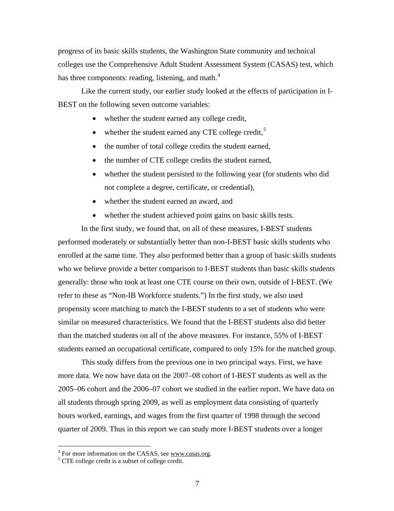
progress of its basic skills students, the Washington State community and technical

colleges use the Comprehensive Adult Student Assessment System (CASAS) test, which

has three components: reading, listening, and math.4

Like the current study, our earlier study looked at the effects of participation in I-

BEST on the following seven outcome variables:

• whether the student earned any college credit,

• whether the student earned any CTE college credit,5

• the number of total college credits the student earned,

• the number of CTE college credits the student earned,

• whether the student persisted to the following year (for students who did

not complete a degree, certificate, or credential),

• whether the student earned an award, and

• whether the student achieved point gains on basic skills tests.

In the first study, we found that, on all of these measures, I-BEST students

performed moderately or substantially better than non-I-BEST basic skills students who

enrolled at the same time. They also performed better than a group of basic skills students

who we believe provide a better comparison to I-BEST students than basic skills students

generally: those who took at least one CTE course on their own, outside of I-BEST. (We

refer to these as “Non-IB Workforce students.”) In the first study, we also used

propensity score matching to match the I-BEST students to a set of students who were

similar on measured characteristics. We found that the I-BEST students also did better

than the matched students on all of the above measures. For instance, 55% of I-BEST

students earned an occupational certificate, compared to only 15% for the matched group.

This study differs from the previous one in two principal ways. First, we have

more data. We now have data on the 2007–08 cohort of I-BEST students as well as the

2005–06 cohort and the 2006–07 cohort we studied in the earlier report. We have data on

all students through spring 2009, as well as employment data consisting of quarterly

hours worked, earnings, and wages from the first quarter of 1998 through the second

quarter of 2009. Thus in this report we can study more I-BEST students over a longer

4 For more information on the CASAS, see www.casas.org. 5 CTE college credit is a subset of college credit.

7

span of time, using the same outcomes that we used in the first report. In addition, we

examine two employment outcomes, namely whether or not there was any change in

students’ wages after participation in I-BEST and average hours worked after leaving the

program. The second difference is that in this study we use a difference-in-differences

methodology to examine the effects of I-BEST on student outcomes to account for the

fact that I-BEST students may differ in unobserved ways from other basic skills students.

The differences between the previous study and this study are summarized in Table 2.

Table 2 Comparison Between the Previous I‐BEST Study 

(Jenkins, Zeidenberg, & Kienzl, 2009) and the Current Study 

  Previous Study  Current Study Cohorts Studied  2006–07  2006–07 and 2007–08 Cohorts Studied Through  2007–08  2007–08 and 2008–09 Number of Students in Sample  31,078  77,147 Number of I‐BEST Students  896  1,390 CASAS Score Included as a Control  No  Yes Logistic Regression Analysis  Yes  Yes Propensity Score Matching Analysis  Yes  Yes College Credit Outcomes   Yes  Yes Persistence Outcome  Yes  Yes Award Outcome  Yes  Yes Basic Skills Test Gain Outcome  Yes  Yes Labor Market Outcomes  Yes  Yes Causal (Difference‐in‐Differences) Analysis  No  Yesa 

aThe causal analysis also uses the 2005–06 cohort. 

3. Findings from Multivariate Analyses

We first present the descriptive statistics comparing I-BEST students to two other

groups: Non-IB Workforce students (basic skills students who took at least one CTE

course, but not I-BEST), and Non-IB Non-Workforce students (basic skills students who

took no college-level CTE courses during their first year).6 We then describe the results

of multivariate analyses estimating the effect of I-BEST for each outcome examined here.

6 Note that Non-I-BEST Non-Workforce students could have taken a non-CTE college course.

8

3.1 Descriptive Characteristics and Outcomes

For this analysis, we obtained data on 89,062 students who took a basic skills

course in a Washington State community or technical college in 2006–07 or 2007–08. To

compare outcomes for students who entered college at the same time, we excluded

students who had prior college education (including those with any prior college credits,

degrees, or credit from dual high school-college enrollment courses). This reduced the

sample size to 77,147. Of these, 1,390 were I-BEST students. The 2006–07 entering

cohort had 38,305 students, and the 2007–08 entering cohort had 38,842 students. There

were 608 first-time students who enrolled in I-BEST in 2006–07 and 782 first-timers

enrolled in I-BEST in 2007–08.

In 2006–07, there were 3,583 first-time Non-IB Workforce students, basic skills

students who did not enroll in I-BEST but took a CTE college course on their own, and

2,619 such students in 2007–08. As mentioned, we believe that this subgroup of basic

skills students is most comparable to the I-BEST students because they, like the I-BEST

students, indicated a desire to pursue at least some occupational training by enrolling in a

CTE course. Unlike the I-BEST students, however, the Non-IB Workforce students did

not take the CTE course as part of an integrated program that incorporates basic skills

instruction. The third group of students took no CTE course, either through I-BEST or on

their own. This group, referred to as the Non-IB Non-Workforce students, includes by far

the largest number of basic skills students, since taking a CTE course, whether through I-

BEST or otherwise, is relatively rare.

Table 3 shows that the Non-IB Workforce students have CASAS scores that are

similar to those of the I-BEST students (with a notable difference in the listening score)

and somewhat higher than the average for the entire basic skills student population

(especially on reading and listening). This reinforces our belief that the Non-IB

Workforce students provide a good comparison group for the I-BEST students.

Table A.1 (see Appendix A) shows the mean values of the student characteristics

used as control variables in the regressions and the propensity score matching for each

9

outcome. We also included CASAS scores (means shown in Table 3) as controls.7 As

Table 3 shows, in many ways, the I-BEST students in our sample were similar to other

basic skills students. Some differences, however, are worth noting. I-BEST students were

more likely to be ABE-GED students (as opposed to ESL)—over three quarters of them

are. Significantly more of them received financial aid (we have one general measure of

this and three measures of participation in particular programs). This is partially because

I-BEST program administrators are encouraged to help their students apply for financial

aid, since many of them have low incomes and are not accustomed to paying college

tuition and fees, as they must do for the credit portion of I-BEST.8 I-BEST students were

more likely to be welfare (TANF) participants. They were more likely to be female, less

likely to be Hispanic, and somewhat more likely to be Black. They were much more

likely to enroll full-time. (Higher rates of financial aid may make this possible.) They

were also more likely to be single parents.

Table 3 Means of Earliest CASAS Scores: First Time Basic Skills Students, 

2006–07 and 2007–08  

 I‐BEST  Non‐IB Workforce Students 

Non‐IB Non‐Workforce Students 

 n 

MedianScore 

n  Median Score  n  Median Score 

  1,390    6,202    69,555   

CASAS Math  1,014  225  2,708  224  22,073  222 

CASAS Reading  1,239  235  3,151  233  49,946  217 

CASAS Listening  314  218  691  211  25,060  204   Note: Scores are the earliest on each test, when the test is taken multiple times. 

7 Where CASAS scores are missing, we set the score to missing and set an associated dummy variable to one to indicate the missing value. This is a technique commonly used in econometrics when there are missing test scores (Puma et al., 2009). 8 Basic skills courses in Washington State and the basic skills portion of I-BEST programs are offered for a modest fee of $25 per quarter, but this fee is waived when a student is enrolled in I-BEST. In contrast, students have to pay tuition for college-level CTE courses and the CTE part of I-BEST courses.

10

There were also some noteworthy similarities and differences between the I-

BEST students and the Non-IB Workforce students. We have already noted that they had

similar CASAS scores, higher than those of the basic skills population at large. Both

groups were dominated by ABE-GED students, as opposed to ESL students; the overall

population has more ESL students. Both groups were also much more likely to indicate

an intent to enroll in CTE courses when they registered for college, a goal which they are

working to fulfill. Both groups had similar rates of participation in TANF, higher than the

basic skills population at large. And students in both groups were more likely to be single

parents. One notable difference is that the I-BEST students were about the same age as

their Non-IB Non-Workforce peers and about four years older than the Non-IB

Workforce students.

3.2 Estimates of the Probability of Earning College Credit

Table 4 shows the estimates, from logistic regression, of the differences in the

probabilities of earning college credit of I-BEST and Non-IB Workforce students relative

to the baseline group, Non-IB Non-Workforce students.9 (This baseline group was used

for all of the regressions described here.) Overall, I-BEST students were 56 percentage

points more likely to earn college credit than the baseline group. I-BEST ABE-GED

students were 65 percentage points more likely, and I-BEST ESL students 39 percentage

points more likely, to earn college credit.

Table 4 also shows that Non-IB Workforce students had a probability of earning

college credit that was 17 percentage points higher than the baseline group. The figures

for the ABE-GED and ESL subgroups of the Non-IB Workforce students exceeded the

baseline average by 27 and 13 percentage points, respectively. Thus, Non-IB Workforce

students did significantly better than the baseline group, but not as well as I-BEST

students.

9 These probability estimates are marginal effects from the logistic regression estimated at the means of the control variables (see Kennedy, 2003). They can be thought of as the changes in probability associated with changing from one group to another, when the other covariates are at their means.

11

Table 4 Logistic Regression Estimates of Differences in Probabilities of Selected Outcomes of 

First‐Time I‐BEST Students and First‐Time Non‐IB Workforce Students Relative to First‐Time Non‐IB Non‐Workforce Students 

 

   First‐Time I‐BEST Students 

First‐Time Non‐IB Workforce Students     

Outcome  Group  Diff.  S.E.  Sig. Level  Diff.  S.E  Sig. Level Pseudo‐

R2 N 

All  0.56  0.03  ***  0.17  0.01  ***  0.51  51,149 ABE‐GED 

0.65  0.03  ***  0.27  0.01  ***  0.47  23,570 Received College Credit 

ESL  0.39  0.07  ***  0.13  0.02  ***  0.57  27,552 

All  0.54  0.03  ***  0.19  0.01  ***  0.53  51,149 ABE‐GED 

0.66  0.03  ***  0.27  0.01  ***  0.50  23,570 Received CTE College Credit 

ESL  0.34  0.06  ***  0.15  0.02  ***  0.58  27,055 

All  0.13  0.02  ***  0.21  0.01  ***  0.16  51,149 ABE‐GED 

0.12  0.02  ***  0.16  0.01  ***  0.18  23,570 Persisted to Next Year 

ESL  0.02  0.05  not significant 0.25  0.02  ***  0.15  27,555 

All  0.26  0.03  ***  0.03  0.00  ***  0.56  47,213 ABE‐GED 

0.26  0.03  ***  0.04  0.01  ***  0.52  21,320 Received Award 

ESL  0.21  0.05  ***  0.02  0.01  ***  0.63  24,179 

All  0.19  0.02  ***  0.07  0.01  ***  0.10  51,149 ABE‐GED 

0.17  0.02  ***  0.06  0.01  ***  0.06  23,570 Achieved Basic Skills Point Gain 

ESL  0.21  0.05  ***  0.09  0.02  ***  0.13  27,552   *p < 0.10; **p < 0.05; ***p < 0.01. 

Using the regression results and holding the values of the other variables in the

regression at their means for the full sample of basic skills students, we obtained adjusted

estimates for the probabilities of earning college credit, as shown in Table 5. These

estimates were 57% for I-BEST students, 18% for Non-IB Workforce Students, and 1%

for the Non-IB Non-Workforce students. This method allows us to compare the three

groups while adjusting for differences in characteristics between the groups.

      

12

Table 5 Regression‐Adjusted Estimates of Probabilities of Outcomes for First‐Time I‐BEST, 

Non‐I‐BEST Workforce, and Non‐I‐BEST Non‐Workforce Students  

Outcome  I‐BEST Non‐IB 

Workforce Non‐IB 

Non‐WorkforceReceived College Credit  0.57  0.18  0.01 

Received CTE College Credit  0.55  0.18  0.01 

College Credits Earned  18.2  9.1  1.1 

CTE College Credits Earned  17.2  7.6  0.5 

Persisted to Next Year  0.40  0.48  0.28 

Received Award  0.26  0.03  0.00 

Achieved Basic Skills Point Gain  0.53  0.40  0.33 

Difference in Log Wages (Post‐Prior)  ‐0.03  ‐0.02  ‐0.04 

Difference in Adjusted Quarterly Hours Worked (Post‐Prior)  ‐17.54  ‐24.06  ‐20.83 

Table 6 shows the estimates of the difference in the probability of earning college

credit between I-BEST students and matched “control” students selected by the PSM

method.10 By this method, the difference in probability was 33 percentage points. As

shown in Figure 1, the mean probability was 84% for the I-BEST students and 51% for

the matched students. We cannot directly compare the PSM results to the regression

results because they use different methods, but the fact that both methods produce highly

significant and positive results adds robustness to our study. As we indicate in Appendix

B, there are reasons to have more confidence in the PSM results. As noted above, the

characteristics used to generate the propensity score for each student are the same

characteristics that were used in the regressions, and their means are shown in Table A.1.

The difference in probability of earning college credit between the I-BEST

students and Non-IB workforce students was 40 percentage points, close to the PSM

result of 33%. This value of 40 percentage points represents the difference between the

57 percentage points and the 18 percentage points given above, when rounding is

accounted for. Since this value is similar to the 33% difference found by PSM, this

suggests that the PSM method is selecting from the entire population of basic skills

students a comparison group similar to the Non-IB Workforce students.

10 The quality of a particular PSM is often measured by the degree of “balance,” that is, the extent to which the means of the treated and matched “controls’ are close on the means of known covariates. In this case, there were 65 covariates, and 51 of them showed improved balance as a result of the matching; the remaining 14 showed worsened balance.

13

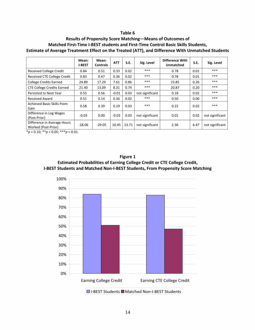
Table 6 Results of Propensity Score Matching—Means of Outcomes of  

Matched First‐Time I‐BEST students and First‐Time Control Basic Skills Students,  Estimate of Average Treatment Effect on the Treated (ATT), and Difference With Unmatched Students 

 

 

Mean: I‐BEST 

Mean: Controls 

ATT  S.E.  Sig. Level Difference With Unmatched 

S.E.  Sig. Level 

*p < 0.10; **p < 0.05; ***p < 0.01.

Received College Credit  0.84  0.51  0.33  0.02  ***  0.78  0.01  *** 

Received CTE College Credit  0.83  0.47  0.36  0.02  ***  0.78  0.01  *** 

College Credits Earned  24.89  17.29  7.61  0.86  ***  23.85  0.26  *** 

CTE College Credits Earned  21.40  13.09  8.31  0.74  ***  20.87  0.20  *** 

Persisted to Next Year  0.55  0.56  ‐0.01  0.03  not significant  0.18  0.02  *** 

Received Award  0.51  0.14  0.36  0.02  ***  0.50  0.00  *** Achieved Basic Skills Point Gain 

0.58  0.39  0.19  0.03  ***  0.22  0.02  *** 

Difference in Log Wages (Post‐Prior) 

‐0.03  0.00  ‐0.03  0.03  not significant  0.01  0.02  not significant 

Difference in Average Hours Worked (Post‐Prior) 

‐18.06  ‐29.05  10.45 13.71 not significant  2.36  6.47  not significant 

Figure 1 Estimated Probabilities of Earning College Credit or CTE College Credit, 

I‐BEST Students and Matched Non‐I‐BEST Students, From Propensity Score Matching 

100%

90%

80%

70%

60%

50%

40%

30%

20%

10%

0%

Earning College Credit Earning CTE College Credit

Matched Non‐I‐BEST Students I‐BEST Students

14

3.3 Estimates of the Probability of Earning CTE College Credit

Table 4 shows the logistic regression estimates of earning CTE college credit.

Note that all students earn as many or fewer CTE college credits than college credits

because CTE credit is a type of college credit. I-BEST students had a probability of

earning CTE college credit that was 54 percentage points higher than the probability for

the baseline group. The two subgroups of I-BEST students, ABE-GED and ESL students,

were respectively 66 and 34 percentage points more likely than the baseline group to earn

CTE credit.

As was the case for earning college credit, the Non-IB Workforce students

performed better than the baseline group but worse than the I-BEST students. They had a

probability of earning CTE college credit that was 19 percentage points higher than the

probability for the baseline group. The ABE-GED subgroup did 27 percentage points

better than the corresponding subgroup in the baseline group, while the ESL subgroup did

15 percentage points better.

Holding the other variables at their means, we used the regression to calculate

adjusted point estimates of the probabilities for each group. The results are shown in

Table 5. We estimated that 55% of I-BEST students would earn CTE college credit, as

opposed to 18% of Non-IB Workforce students and 1% of Non-IB Non-Workforce

students.

The PSM results are shown in Table 6. Using this method, we found a difference

of 36 percentage points between I-BEST students and matched controls. As shown in

Figure 1, the mean probability of earning CTE credit was 83% for the I-BEST students

and 47% for the matched students. This 36 percentage point difference is very similar to

the 37 percentage point difference between I-BEST students and Non-IB Workforce

students estimated by regression, indicating that our results are robust.

3.4 Estimates of the Number of Credits Earned

As shown in Table 6, ordinary least squares (OLS) regression finds that I-BEST

students earned 17.1 more college credits and 16.6 more CTE credits than the baseline

group. ABE-GED I-BEST students earned 18.1 more college credits and 17.8 more CTE

15

college credits than the corresponding baseline group. For the ESL I-BEST subgroup, the

corresponding figures were 12.2 and 12.0.

Table 6 OLS Regression Estimates of Differences in Selected Outcomes for First‐Time I‐BEST  

and First‐Time Non‐IB Workforce Students Relative to First‐Time Non‐IB Non‐Workforce Students  

   First‐Time I‐BEST Students 

First‐Time Non‐IB Workforce Students     

Outcome  Group  Diff.  S.E.  Sig. Level  Diff.  S.E  Sig. Level  R2  N 

All  17.1  0.8  ***  8.0  0.3  ***  0.4  51,149 

ABE‐GED  18.1  1.0  ***  7.9  0.4  ***  0.4  23,573 

College Credits Earned 

ESL  12.2  1.2  ***  6.8  0.6  ***  0.4  27,555 

All  16.6  0.7  ***  7.0  0.3  ***  0.3  51,149 

ABE‐GED  17.8  0.9  ***  7.0  0.3  ***  0.3  23,573 

CTE College Credits Earned 

ESL  12.0  1.0  ***  6.0  0.5  ***  0.3  27,555 

All  0.01  0.02  not significant  0.01  0.01  not significant  0.0  15,146 

ABE‐GED  0.01  0.02  not significant  0.01  0.01  not significant  0.0  9,877 

Difference in Log Wages (Post‐Prior) 

ESL  ‐0.01  0.03  not significant  0.02  0.03  not significant  0.0  5,262 

All  3.1  8.1  not significant  ‐3.2  4.5  not significant  0.0  15,144 

ABE‐GED  7.5  9.6  not significant  ‐5.6  5.2  not significant  0.0  9,875 

Difference in Average Quarterly Hours Worked (Post‐Prior) 

ESL  ‐4.0  16.5  not significant  ‐2.3  10.4  not significant  0.0  5,262 *p < 0.10; **p < 0.05; ***p < 0.01. 

The Non-IB Workforce students earned eight more college credits and seven

more CTE credits than the baseline group. The ABE-GED subgroup also earned eight

more college credits and seven more CTE credits than the corresponding subgroup of the

baseline group. The corresponding figures for the ESL subgroup were seven and six.

Using our regression model and setting the values of the control variables at their

means, we calculated regression-adjusted point estimates for the mean number of college

credits and CTE credits earned, as shown in Table 5. On average, I-BEST students earned

18 college credits and 17 CTE credits; Non-IB Workforce students earned 9 college

credits and 8 CTE credits. Non-IB Non-Workforce students earned 11 college credits and

about half of one CTE college credit.

The PSM method, as shown in Table 6, found that the I-BEST students earned 8

college credits and 8 CTE college credits more than the matched group. As shown in

Figure 2, the I-BEST students earned 25 college credits and 21 CTE college credits on

16

average; for the matched group, the corresponding figures are 17 and 13. Note that the

differences found by PSM are very similar to the corresponding differences of 9 and 10

credits found using OLS to compare the I-BEST and Non-IB Workforce students,

indicating that the result is robust.

3.5 Estimates of the Probability of Persisting into the Next Year

For students in each cohort (2006–07 or 2007–08), we determined whether or not

they persisted as a student in the following year. Persistence was defined as either

enrolling in a course or obtaining an award. Those who received an award are considered

persisting to avoid penalizing programs whose students leave because they receive an

award.

As shown in Table 4, logistic regression found that I-BEST students were 13

percentage points more likely than the baseline group to persist. The ABE-GED subgroup

was 12 percentage points more likely to persist. There was no significant difference in

persistence from the baseline for the ESL group.

This was the only outcome variable on which the Non-IB Workforce students

performed better than their I-BEST peers. They were 21 percentage points more likely to

persist than the baseline group. Their ABE-GED subgroup was 16 percentage points

more likely to persist than the corresponding subgroup of the baseline group; the figure

for the ESL subgroup was 25 points.

We used our logistic regression model with the controls held at their means to

estimate regression-adjusted means for each of the three groups, as shown in Table 5. I-

BEST students had a 40% probability of persisting, Non-IB Workforce students had a

48% probability, and Non-IB Non-Workforce students had a 28% probability.

As shown in Table 6 and Figure 3, the PSM model did not find a statistically

significant difference in persistence between the I-BEST and matched students. (The I-

BEST students had a higher rate, but the difference was not significant.) Thus we have

not found any relationship between participation in I-BEST and persistence.

17

Figure 2 Number of College Credits and CTE College Credits Earned, 

 I‐BEST Students and Matched Non‐I‐BEST Students, From Propensity Score Matching 

30

25

20

15

10

5

0CTE College Credits Earned College Credits Earned

Matched Non‐I‐BEST Students I‐BEST Students

Figure 3 Rates of Persistence and of Award Receipt, I‐BEST Students and Matched Non‐I‐BEST Students, From Propensity Score Matching

100%

90% 

80% 

70% 

60% 

50% 

40% 

30% 

20% 

10% 

0%Persisted to Next Year Received Award 

I‐BEST Students Matched Non‐I‐BEST Students 

18

3.6 Estimates of the Probability of Earning an Award

Table 4 shows the logistic regression estimates of the probability of earning an

award, relative to the baseline group. (As we have seen, the vast majority of awards

earned by basic skills students are certificates, not degrees.)

I-BEST students were 26 percentage points more likely to earn an award than the

baseline group. The ABE-GED subgroup was 26 percentage points more likely to earn an

award; the ESL subgroup, 21 percentage points more likely.

Non-IB Workforce students were 3% more likely to earn an award than the

baseline group. Among them, the ABE-GED subgroup was 4% more likely, and the ESL

subgroup 2% more likely, to earn an award.

We used the logistic regression model to estimate adjusted means for the three

groups by setting the controls at their means to eliminate measured differences between

the groups. As shown in Table 5, using this method, the I-BEST students were estimated

to have a 26% chance of getting an award; the Non-IB Workforce students had a 3%

chance, and the Non-IB Non-Workforce students had a negligible chance.

Table A.2 (see Appendix A) shows the marginal effects from the regression.

While quite a few variables in the specification were statistically significant, only the I-

BEST and non-I-BEST-workforce dummies had any substantial relationship with the

outcome.

The PSM model (shown in Table 6) found that I-BEST students were 36

percentage points more likely than the matched group to obtain an award. Figure 3 shows

that the I-BEST students had a 50% chance of getting an award, whereas the matched

students had a 14% chance. The 36 point difference is larger than the 23 point difference

between the I-BEST and the Non-IB-Workforce students estimated by regression, but

they are both highly significant and in the same direction.

3.7 Estimates of the Probability of Achieving Point Gains on Basic Skills Tests

The fact that students in I-BEST learn basic skills in the context of instruction on

technical subject matter raises the question of whether I-BEST helps students improve

their basic skills. Table 4 shows the logistic regression estimates of the differences in the

probability of achieving point gains on the CASAS basic skills tests used throughout the

19

Washington community college system. As shown in the table, I-BEST students were 19

percentage points more likely to make such gains than the baseline group. This figure

was 17 percentage points for the ABE-GED subgroup and 21 percentage points for the

ESL subgroup. Non-IB Workforce students were 7 percentage points more likely to make

gains than the baseline group. For the ABE-GED subgroup of this group, the figure was 6

percentage points, and for the ESL subgroup, it was 9 percentage points.

Table 5 shows the results of using the logistic regression to estimate the adjusted

means, setting the controls at their means in order to control for systematic differences

between the groups. Following this method, 53% of I-BEST students were found to make

gains, as were 40% of Non-IB Workforce students and 33% of Non-IB Non-Workforce

students.

The PSM results in Table 6 show that I-BEST students were 19 percentage points

more likely than matched students to achieve point gains. Of the matched I-BEST

students, 58% achieved a gain, as opposed to 39% of the matched controls. The 19

percentage point difference is greater than the 13 percentage point difference that was

found between the I-BEST students and the Non-IB-workforce students using logistic

regression; however, both results are highly significant and in the same direction.

3.8 Employment Outcomes

We examined two employment outcomes, the change in the logarithm of real

wages and the change in the average number of hours worked per quarter.

Estimates of the change in the logarithm of real wages. To examine the

relationship between I-BEST enrollment and wages, we used data on real (inflation-

adjusted) wages for the students in the sample. We looked at two periods: a period three

to eight quarters prior to their enrollment in school, and a period three to eight quarters

after.11 We determined the average real wages for each of these periods. For students to

be included in this analysis, they needed to have at least one wage record in each of these

periods. Only 28% of students in our sample had wage records both before and after

enrollment. Note that this was partially due to the fact that about a third of the students 11 Note that we excluded the quarters immediately before and after schooling because there is a well-known effect, known as Ashenfelter’s dip, which is a dip in earnings that begins soon before entering a training program and does not generally start to increase until several quarters after training (Heckman & Smith, 1999).

20

did not provide a social security number (perhaps for privacy reasons, or perhaps because

they lacked one), and without a social security number, a student’s wage records cannot

be identified.

Table A.3 (see Appendix A) shows the differences in observed characteristics

between those students who worked both before and after, and those who did not. Note

that those who worked before and after were more likely to be ABE or GED students (as

opposed to ESL) and less likely to be Hispanic.

We used OLS regression to predict the effect of enrollment in I-BEST on an

outcome that was defined as the change in the logarithm of the wage (the log wage after

minus the log wage before). It is conventional practice in labor economics to use the log

wage as an outcome because wages tend to be not uniformly distributed (Card, 1999). We

found no significant effect of I-BEST on wages. A PSM model also found no significant

effect.

Descriptively, there was actually a small decline in wages for all of the basic

skills students. Their mean wages before entering school were $12.26. After leaving

school, they were $12.16. We believe this decline in wages is due to the unusually deep

recession—the deepest since the Great Depression—that started as these two cohorts of

students were leaving school (Barkley & Davis, 2009). Unemployment in Washington

State started to rise sharply in early 2008.12

Estimates of the change in quarterly hours worked. Basic skills students who

were employed before and after school experienced a decline in average hours worked

during the periods examined to calculate the wage outcome—another probable effect of

the deep recession. Prior to school, these workers worked a mean of 340 hours per

quarter, and after leaving school, they worked a mean of 318 hours per quarter. OLS

regression found no significant effect of I-BEST on this decline in hours worked. Neither

did a PSM model.

We also tested to see if enrollment in I-BEST had any effect on the chances of

employment for those workers that were not employed prior to entering school. We found

no statistically significant effect.

12 The unemployment rate in the state was between 4.4 and 4.6% for all of 2007. In March of 2008, it began to trend upward, to 4.7 percent. By December of 2008, it had reached 6.9 percent, and by December of 2009, 9.2 percent. These figures were obtained from the Bureau of Labor Statistics’ website.

21

4. Difference-in-Differences Analysis

The regression and propensity score matching methods used in the analyses so far

produced similar results. However, although both methods accounted for observed

differences between the treated (I-BEST) and comparison groups, neither could control

for selection bias that may be due to unobserved differences between the groups. Some

unobserved differences could have been related to the process by which students are

selected into I-BEST programs. Thus, while the results of the above analyses, as well as

our previous study, indicate that participation in I-BEST is correlated with better

educational outcomes over the two-year tracking period, they do not provide definitive

evidence that the I-BEST program caused the superior outcomes.

To address the issue of selection bias, we conducted a difference-in-differences

(DID) analysis. We compared the overall change in outcomes at schools that

implemented I-BEST to the overall change in outcomes at schools that had not yet

implemented the program during the same time, thus effectively “differencing out” the

pre-intervention student characteristics. Any time-invariant individual characteristics are

removed when we find the difference between post- and pre-intervention outcomes.

4.1 Sample

In this analysis, we exploited the fact that 14 new Washington State colleges

started offering the I-BEST initiative in the 2006–07 academic year and used information

from the students who were in these new institutions to compare with new students who

did not have I-BEST in these same institutions in the 2005–06 academic year.13 We

limited our sample to students who were considered to be “basic skills” students, that is,

students who initially enrolled in adult basic education, English-as-a-second-language, or

GED courses at their initial college of enrollment. We further limited the sample to those

students who enrolled in I-BEST or a non-I-BEST workforce course in 2005–06 or 2006–

07, since both groups indicated a desire to pursue college-level CTE education by taking

a CTE course and because, as discussed, these two groups are more similar to one

another in their average CASAS scores and other key respects than to basic skills

13 Note that we did not use the 2005–06 data for the regression and PSM analyses, because 2005–06 was still a pilot year for I-BEST. Here, we use 2005–06 data for only those 24 colleges that did not have I-BEST in that year because it is important for the difference-in-differences analysis.

22

students who do not take a CTE course. Thus, these students were more likely to be

affected by the change in I-BEST policies than the rest of the basic skills student

population. We defined treatment exposure by cohort, or the year of first-time entry into a

Washington State community or technical college. As a control group, we used data from

the 10 colleges that did not have I-BEST in their institutions until the 2007–08 academic

year. By observing students in the control group institutions in the 2005–06 and 2006–07

academic years, we have an entirely untreated group that we can measure against using

data on students in the 14 colleges that started I-BEST in 2006–07.

In the 2005–06 academic year, only 10 two-year colleges in Washington State

implemented I-BEST programs. In the 2006–07 year, 14 new colleges offered I-BEST

programs, bringing the total to 24 colleges. By the year 2007–08, all 34 Washington State

community and technical colleges offered I-BEST programs. The four outlined boxes in

Table 7 represent the colleges (Group B and Group C) and cohorts (2005–06 and 2006–

07) that are of interest in this difference-in-differences analysis:

Table 7  Timing of Introduction of I‐BEST in Washington State’s 

34 Community and Technical Colleges  

 2005‐06  2006‐07  2007‐08 

Group A Colleges  10  10  10 

Group B Colleges    14  14 

Group C Colleges      10 

 

 

The group B and C comparison is relevant because it is the only place in the grid

in which the policy (I-BEST) was introduced in one group of colleges (B) while it had

not yet been introduced in another (C). A situation like this is necessary to carry out a

difference-in-differences analysis, because one is assuming for the purposes of the

23

analysis that any variation over time not due to the policy is the same in both groups, and

that the only difference between the groups was due to the policy.

Enrollment in I-BEST in each academic year, separated by college group, is

illustrated here, in Figure 4:14

Figure 4 Enrollment in I‐BEST in Group B and C Colleges, 2005–06 Through 2007–08 

 

Group CGroup B

I‐BE

ST Enrollm

ent 

Academic Year2007–082006–072005–06 

35.00%

30.00%

25.00%

20.00%

15.00%

10.00%

5.00% 

0.00% 

 

 

Among students enrolled in a Group B college, enrollment increased to 424

students by the 2006–07 academic year, with 17% of basic skills students taking at least

one CTE course. By the 2007–08 academic year, 701 students in a Group B college

enrolled in I-BEST, compared to 187 students in a Group C college.

14 Students with spurious enrollments in I-BEST were dropped from the sample. A total of 83 students were listed as being enrolled in I-BEST in 2005–06 in a Group B college, and 44 students were listed as being enrolled in I-BEST in 2006–07 in a Group C college. The denominator of each percentage calculation was the number of I-BEST and Non-IB Workforce students in each box (e.g., Group B, cohort 2006–07).

24

4.2 Methodology

Any statistically significant “differences in differences”—that is, changes in pre-

and post intervention outcomes in the 14 “Group B” colleges (which began to formally

offer I-BEST in 2006–07) compared with changes in student outcomes in the 10 “Group

C” colleges (which did not offer I-BEST until 2007–08)—can be attributed to the I-BEST

interventions under the assumption that the changes in student outcomes the Group B

colleges would have exhibited a similar trend as the changes observed during that time

period in the Group C colleges, had the Group B colleges not implemented I-BEST. With

this assumption, the difference-in-differences method addresses the selection bias

limitations of the regression and propensity score matching methods used in the analyses

of I-BEST outcomes presented in the previous section.15 As we have information on both

the intent to treat (the fact that the students are in the 14 new colleges in 2006–07) and

the actual receipt of treatment (the fact that some of these students actually enrolled in I-

BEST of their own accord), we are able to run separate regressions using these two

groups.

In the first regression, we modeled our intent-to-treat framework much like

Dynarski did with her HOPE study (2000) by comparing outcomes before and after I-

BEST was introduced, both within colleges that implemented I-BEST and those that did

not. We first indicated basic skills students who were in one of the 14 new colleges

(GroupBi) as those who were newly eligible for participation in I-BEST. We also added a

dummy variable for students in the 2006–07 cohort (2006–07i) to indicate those in the 14

new colleges who were newly eligible for I-BEST strictly due to timing. We then added

an interaction term for which the coefficient will indicate the effect of being in a school

and year in which I-BEST was offered on student outcomes for basic skills students

seeking CTE. We also added a vector of student and institutional characteristics (Xi):

1) yi = β0 + β1 GroupBi + β2 2006–07i + β3 (GroupBi * 2006–07i) + Xi β4 + vi

15 There are, however, some alternative hypotheses that could potentially violate this assumption, including the recruitment of high-achieving students into I-BEST programs and the implementation of other reforms concurrent with I-BEST implementation, among others.

25

Outcomes (yi) included certificate and associate degree completion as well as

college credits earned. The coefficient β3 captures the impact estimate of the colleges’

intent to treat. β1 controls for pre-existing differences between schools that did or did not

implement I-BEST, and β2 controls for cohort differences that are observed for all

institutions in the Washington State community and technical college system.

We used information on only the 2005–06 and 2006–07 cohorts, limiting the

sample to only the students in the 14 colleges that began to implement I-BEST in 2006–

07 (the 2005–06 and 2006–07 cohorts in Group B colleges) and the students in the 10

colleges that did not have I-BEST in 2005–06 and 2006–07 (the 2005–06 and 2006–07

cohorts in Group C colleges). The 10 colleges comprise a “clean” control group against

which we can measure the effects of I-BEST, as the students in these colleges were not

subject to I-BEST within this time frame. The coefficient β3 will identify the effect of the

colleges’ intent to offer I-BEST on student outcomes.

4.3 Results

The results shown in Table A.4 (see Appendix A) capture the intention to treat

our target sample of basic skills students seeking CTE through eligibility to participate in

I-BEST. Using difference-in-differences, we measure the difference between being in a

Group B college and being in a Group C college, both before and after I-BEST eligibility

as measured by the 2005–06 cohort (when neither Group B nor Group C colleges offered

I-BEST) versus the 2006–07 cohort (when Group B colleges began offering I-BEST). We

used ordinary least squares (OLS) estimates to measure the effect of I-BEST on

certificate and degree attainment as well as on college credits received. We checked these

results with marginal probit estimates for robustness.16

Our results indicate that students who were eligible for I-BEST (i.e., those who

were in Group B colleges in 2006–07) were about 10 percentage points more likely to

obtain college credits than to those who were not (i.e., those who were in Group C

colleges), and the results were statistically significant at the five-percent level. I-BEST

eligibility had a positive effect on earning an occupational certificate by 7.4 percentage

16 OLS and marginal probit outcomes were similar in nearly all cases. The probit results are given in Table A.5 (see Appendix A).

26

points, a result that was statistically significant at the ten-percent level. There were no

indications, however, that I-BEST had an effect on associate degree attainment.

We also performed the difference-in-differences analysis on the same two

employment outcomes that we looked at earlier, the difference between log wages earned

after leaving school and before entering school and the corresponding difference in the

average quarterly hours worked. We did not find any indications that I-BEST had an

effect on these, which is the same result we found with the regression and propensity

score models.

4.4 Enrollment as a Measure of Take-Up

We conducted a second set of regressions using the same sample used to produce

the results in Table A.4 and exploiting data on which students actually enrolled in I-

BEST and thus received the treatment. This allowed us to measure the effect of treatment

by enrollment, given that these students voluntarily accepted the offer to join I-BEST.

The variables used are the same as for the DID analysis, save for a dummy dependent

variable indicating that the student actually enrolled in I-BEST within two years in one of

the 14 new colleges through enrollment (Ei). The resulting first-stage equation predicts I-

BEST enrollment:

2) Ei = β0 + β1 GroupBi + β2 2006–07i + β3 (GroupBi * 2006–07i) + Xi β4 + vi

The results are shown in Table A.6 (see Appendix A).

Among the students in our targeted sample, our results indicate that attending a

school that offered I-BEST increased enrollment in I-BEST by 17 percentage points. This

indicates that simply being eligible for I-BEST is a good predictor for actually enrolling

in it. From a policy perspective, this is a promising indication that the intent to treat these

students through I-BEST actually leads to treatment, by way of student enrollment.

27

5. Conclusion

As in our earlier quantitative study of I-BEST (Jenkins, Zeidenberg, & Kienzl,

2009), the regression and propensity score analyses conducted with a larger sample of

students over a longer time period showed positive relationships between participation in

I-BEST and various desirable outcomes. Many of the relationships are striking: I-BEST

students earned substantially more college credits (both total and CTE) than their peers,

were much more likely to earn an award, and were moderately more likely to achieve a

basic skills gain. The only outcome under study on which I-BEST students did not do

better than the Non-IB Workforce students was persistence, and even on that outcome, I-

BEST did better than the Non-IB Non-Workforce students. These results are robust with

respect to the two methodologies of regression and propensity score matching. Although

there is reason to believe that the latter method does a better job in accounting for

selection bias, neither of these techniques can eliminate it in the presence of unobserved

(and perhaps unobservable) factors, such as student motivation, that may be influencing

the outcomes and are not controlled for.

As we have seen, the I-BEST students in our sample received financial aid at

significantly higher rates than other basic skills students, which is not surprising because

we found through qualitative work reported in a companion study that colleges have

actively sought to help I-BEST students get financial aid. Over half (58%) of I-BEST

students received some form of financial aid, as opposed to 21% of Non-IB Workforce

students and only 2% of Non-IB Non-Workforce students (this last group probably

received little aid because they did not take college-level courses at all and therefore did

not need and were not eligible for aid). Thus, it is possible that the positive effects of I-

BEST are due not to the program content or structure but to the improved access to

financial aid that allows students to progress. Washington State’s Opportunity Grants, in

particular, were targeted at I-BEST students. Unfortunately, we are unable to disentangle

the effects of financial aid and the program itself because improving access to financial

aid is part of the design of I-BEST.

To measure the causal effects of the intention to treat basic skills students with the

I-BEST program, we employed a difference-in-differences strategy, taking advantage of

28

the fact that different colleges in the Washington community and technical college

system began implementing the program at different times. That analysis revealed a 10

percentage point increase in the likelihood that targeted students would earn at least one

college credit if they were eligible for the program. Simply being in a cohort enrolled in a

group of colleges that offered I-BEST also increased the likelihood of earning an

occupational certificate within three years by over seven percentage points. When

students were exposed to this program, there was a direct and statistically significant

relationship to their actual enrollment in it, which further supports our finding of a causal

relationship between I-BEST and positive student outcomes. This finding is especially

impressive because it represents an estimate of the effect on student outcomes of I-BEST

programs during their first year of implementation at the colleges that provided the

treatment in our analysis. It is likely that these colleges have been able to improve their

delivery of the I-BEST model as they have gained experience with it over time.

We were not able to find any relationship between I-BEST and positive wage

changes or average hours worked after leaving the program. However, the students in our

sample exited the program just as a major recession was starting, which might explain the

lack of labor market benefits of I-BEST in the period under study. Given that I-BEST

students are more likely than similar students to earn postsecondary credentials and that

workers with such credentials have historically had an advantage in the labor market, we

expect that I-BEST students will fare better than students in the comparison groups as the

Washington State labor market recovers.

In a parallel study to this quantitative analysis of I-BEST outcomes, we

interviewed faculty, staff, and administrators involved with I-BEST at all 34 Washington

State community and technical colleges to find out how I-BEST programs operate and to

learn about common challenges and promising practices in implementing programs based

on the I-BEST model. The findings from that study are presented in a companion report

(Wachen, Jenkins, Van Noy, et al., 2010).

In the next phase of research on I-BEST (to be carried out in 2011), CCRC will

conduct field research to examine the practices of I-BEST programs that are found

through quantitative analysis to have superior outcomes (controlling for student and

institutional characteristics). This planned research should provide further insight into

29

what makes I-BEST programs effective in helping basic skills students enter and succeed

in postsecondary CTE programs.

30

Appendix A: Tables

Table A.1 Characteristics of First Time Basic Skills Students, 2006–07 and 2007–08 

 

  I‐BEST  Non‐IB Workforce 

Non‐IB Non‐Workforce 

Number of Students in Program  1,390  6,202  69,555  Program Classification ABE/GED Student  76.28%  80.18%  47.24% 

ESL Student  23.72%  19.82%  52.76%  Social and Economic Characteristics Mean Age  30.73  26.42  30.24 

Female  62.52%  60.21%  53.17% 

Hispanic  20.72%  17.72%  37.40% 

Black, Non‐Hispanic  11.08%  11.59%  7.58% 

Asian/Pacific Islander  9.86%  8.16%  10.87% 

Single w/ Dependent  21.22%  20.24%  13.24% 

Married w/ Dependent  22.45%  13.59%  22.75% 

Disabled   6.62%  7.30%  3.59% 

Percent of Students in the Lowest Two Quintiles of Socioeconomic Status [1] 

61.56%  55.91%  58.18% 

 Current Schooling Characteristics CTE Intent[2]  71.29%  48.02%  18.02% 

Intent Is Academic  7.12%  8.71%  6.88% 

Received Aid  25.68%  13.96%  1.55% 

Enrolled Full Time  66.83%  57.85%  27.84% 

First Enrolled in 1st Quarter   13.74%  17.35%  14.57% 

First Enrolled in 2nd Quarter  38.35%  46.66%  31.46% 

First Enrolled in 3rd Quarter  27.63%  23.52%  29.06% 

First Enrolled in 4th Quarter  20.29%  12.46%  24.91%  Previous Schooling Characteristics GED  15.11%  11.38%  4.47% 

High School Graduate  37.12%  21.72%  16.59% 

WorkFirst (WA TANF) Participant  40.58%  38.55%  20.95% 

Financial Aid       

       Received a Pell Grant  26.40%  15.21%  0.78% 

       Received an Opportunity Grant  34.32%  2.08%  0.05% 

       Received a State Need Grant  21.87%  13.12%  0.58% 

       Received Any Aid  58.13%  21.33%  2.01% 

Worked While Enrolled  9.06%  5.13%  12.14% Note: [1] This is based on the quintile of the average socioeconomic status of the Census block group in  which the student’s residence is found. For details, see Crosta, Leinbach, and Jenkins (2006) and Washington State Board for Community and Technical Colleges (2006). [2] CTE and academic intent indicate the type of college program the student means to pursue. If CTE, the student intends to pursue workforce training; if academic, the student intends to pursue a program that leads to a degree and/or transfer to a four‐year institution. Students do not always follow their stated intent (see Bailey, Jenkins, & Leinbach, 2006). 

31

Table A.2 Marginal Effects Coefficients for Logistic Regression 

Outcome Variable: Award Within Two Years 

  Coefficient Robust 

Standard Error  P‐value 

I‐BEST Student  0.2625  0.0273  *** 

Non‐I‐BEST Workforce Student  0.0342  0.0041  *** 

Age  0.0000  0.0000  *** 

Estimated SES  0.0000  0.0001   

Received Need‐Based Financial Aid  ‐0.0002  0.0002   

Received Pell Grant  0.0002  0.0004   

Received State Need Grant  0.0003  0.0004   

Received Opportunity Grant  0.0012  0.0005  ** 

Disabled  ‐0.0002  0.0003   

In 06–07 Cohort  0.0000  0.0001   

Single Parent  0.0000  0.0002   

Married Parent  0.0002  0.0002   

Full‐Time Student  0.0009  0.0002  *** 

Female  ‐0.0004  0.0002  *** 

Hispanic  ‐0.0006  0.0002  *** 

Black, Non‐Hispanic  ‐0.0002  0.0002   

Asian/Pacific Islander, Non‐Hispanic  0.0003  0.0003   

CTE Intent  0.0010  0.0003  *** 

Academic Intent  0.0004  0.0004   

GED is Highest Educ.  0.0000  0.0002   

HS Graduate  0.0002  0.0002   

First Enrolled in Quarter 1  0.0002  0.0003   

First Enrolled in Quarter 2  ‐0.0001  0.0002   

First Enrolled in Quarter 3  ‐0.0004  0.0002   

CASAS Math Score  0.0000  0.0000   

CASAS Math Score Missing  0.0013  0.0016   

CASAS Reading Score  0.0000  0.0000  *** 

CASAS Reading Score Missing  0.0117  0.0112   

CASAS Listening Score  0.0000  0.0000  *** 

CASAS Listening Score Missing  0.0094  0.0069   

TANF (Welfare) Recipient  0.0003  0.0002   

Worked While Enrolled  ‐0.0010  0.0002  *** 

College 1  ‐0.0007  0.0008   

College 2  ‐0.0011  0.0005   

College 3  ‐0.0007  0.0009   

College 4  ‐0.0012  0.0004  *** 

College 5  ‐0.0012  0.0005  ** 

College 6  ‐0.0014  0.0003  *** 

College 7  0.0001  0.0017   

College 8  ‐0.0010  0.0006  * 

College 9  0.0083  0.0104   

College 10  ‐0.0007  0.0009   

32

College 11  0.0011  0.0027   

College 12  0.0023  0.0036   

College 13  0.0012  0.0028   

College 15  0.0211  0.0277   

College 16  0.0002  0.0018   

College 17  ‐0.0006  0.0010   

College 18  ‐0.0005  0.0011   

College 19  0.0005  0.0022   

College 20  ‐0.0005  0.0011   

College 22  ‐0.0011  0.0007   

College 23  0.0005  0.0020   

College 25  0.0013  0.0029   

College 26  ‐0.0013  0.0003  *** 

College 27  ‐0.0002  0.0013   

College 28  0.0000  0.0016   

College 30  ‐0.0011  0.0004  *** 

College 31  ‐0.0004  0.0011   

College 32  0.0019  0.0033   

College 33  0.0002  0.0018   

College 34  0.0044  0.0061   

College 35  ‐0.0003  0.0014   *p < 0.10, **p < 0.05, ***p < 0.01.

33

Table A.3 

Comparison Between Students Who Worked Both  Before and After Schooling and Those Who Did Not Do So 

  Worked Both 

Before and After Did Not Do So 

Number of Students  21,967  55,180  Program Classification ABE/GED Student  67.64%  42.77% ESL Student  32.36%  57.23%  Social and Economic Characteristics Mean Age  29.13  30.27 Female  54.75%  53.57% Hispanic  25.57%  39.48% Black, Non‐Hispanic  10.65%  6.89% Asian/Pacific Islander  11.12%  10.44% Single w/ Dependent  16.97%  12.75% Married w/ Dependent  19.92%  22.84% Disabled   3.96%  3.94% 

Percent of Students in the Lowest Two Quintiles of Socioeconomic Status [1]  57.45%  58.33%  Current Schooling Characteristics CTE Intent[2]  24.73%  20.06% Intent Is Academic  8.75%  6.34% Received Aid  5.46%  2.00% Enrolled Full Time  35.71%  29.06% First Enrolled in 1st Quarter   16.85%  13.96% First Enrolled in 2nd Quarter  35.10%  31.89% First Enrolled in 3rd Quarter  27.56%  29.00% First Enrolled in 4th Quarter  20.49%  25.15%  Previous Schooling Characteristics GED  6.76%  4.61% High School Graduate  17.99%  17.13% WorkFirst (WA TANF) Participant  34.45%  18.05% Financial Aid            Received a Pell Grant  4.72%  1.46%        Received an Opportunity Grant  1.71%  0.48%        Received a State Need Grant  4.10%  1.11%        Received Any Aid  8.59%  2.97% Worked While Enrolled  26.59%  5.53% 

Note: See Note for Table A.1. 

34

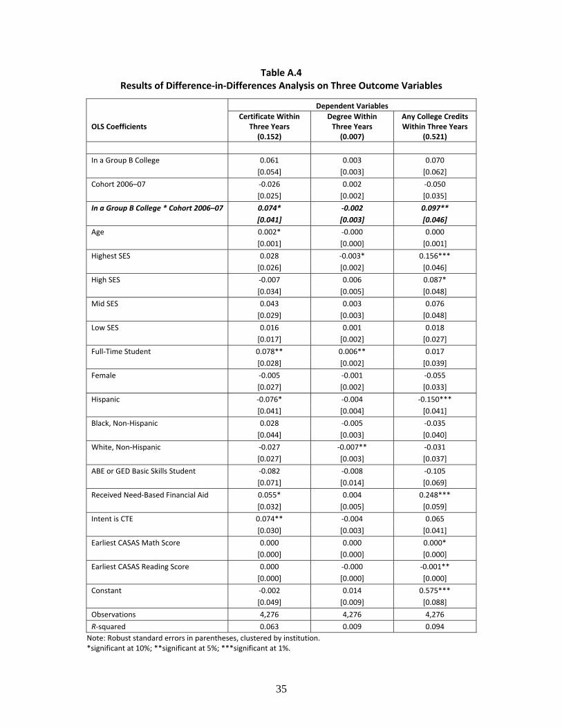
Table A.4 Results of Difference‐in‐Differences Analysis on Three Outcome Variables 

 

   Dependent Variables 

OLS Coefficients Certificate Within 

Three Years (0.152) 

Degree Within Three Years (0.007) 

Any College Credits Within Three Years 

(0.521)         

In a Group B College  0.061  0.003  0.070    [0.054]  [0.003]  [0.062] 

Cohort 2006–07  ‐0.026  0.002  ‐0.050    [0.025]  [0.002]  [0.035] 

In a Group B College * Cohort 2006–07  0.074*  ‐0.002  0.097**    [0.041]  [0.003]  [0.046] 

Age  0.002*  ‐0.000  0.000    [0.001]  [0.000]  [0.001] 

Highest SES  0.028  ‐0.003*  0.156***    [0.026]  [0.002]  [0.046] 

High SES  ‐0.007  0.006  0.087*    [0.034]  [0.005]  [0.048] 

Mid SES  0.043  0.003  0.076    [0.029]  [0.003]  [0.048] 

Low SES  0.016  0.001  0.018    [0.017]  [0.002]  [0.027] 

Full‐Time Student  0.078**  0.006**  0.017    [0.028]  [0.002]  [0.039] 

Female  ‐0.005  ‐0.001  ‐0.055    [0.027]  [0.002]  [0.033] 

Hispanic  ‐0.076*  ‐0.004  ‐0.150***    [0.041]  [0.004]  [0.041] 

Black, Non‐Hispanic  0.028  ‐0.005  ‐0.035    [0.044]  [0.003]  [0.040] 

White, Non‐Hispanic  ‐0.027  ‐0.007**  ‐0.031    [0.027]  [0.003]  [0.037] 

ABE or GED Basic Skills Student  ‐0.082  ‐0.008  ‐0.105    [0.071]  [0.014]  [0.069] 

Received Need‐Based Financial Aid  0.055*  0.004  0.248***    [0.032]  [0.005]  [0.059] 

Intent is CTE  0.074**  ‐0.004  0.065    [0.030]  [0.003]  [0.041] 

Earliest CASAS Math Score  0.000  0.000  0.000*    [0.000]  [0.000]  [0.000] 

Earliest CASAS Reading Score  0.000  ‐0.000  ‐0.001**    [0.000]  [0.000]  [0.000] 

Constant  ‐0.002  0.014  0.575***    [0.049]  [0.009]  [0.088] 

Observations  4,276  4,276  4,276 

R‐squared  0.063  0.009  0.094 Note: Robust standard errors in parentheses, clustered by institution.  *significant at 10%; **significant at 5%; ***significant at 1%. 

35

Table A.5 Probit Results for Comparison with Difference‐in‐Differences Result 

 

   Dependent Variables 

 Certificate Within Three 

Years Degree Within Three 

Years Any College Credits Within 

Three Years    OLS  Probit  OLS  Probit  OLS  Probit 

0.061  0.066  0.003  0.002  0.070  0.072 In a Group B College 

[0.054]  [0.056]  [0.003]  [0.001]  [0.062]  [0.066] 

‐0.026  ‐0.031  0.002  0.001  ‐0.050  ‐0.053 Cohort 2006–07 

[0.025]  [0.031]  [0.002]  [0.001]  [0.035]  [0.038] 

0.074*  0.073*  ‐0.002  ‐0.001  0.097**  0.104** In a Group B College  *     Cohort 2006–07  [0.041]  [0.046]  [0.003]  [0.001]  [0.046]  [0.049] 

0.002*  0.002**  ‐0.000  ‐0.000  0.000  0.000 Age 

[0.001]  [0.001]  [0.000]  [0.000]  [0.001]  [0.001] 

0.028  0.036  ‐0.003*  ‐0.001  0.156***  0.162*** Highest SESa 

[0.026]  [0.028]  [0.002]  [0.001]  [0.046]  [0.047] 

‐0.007  ‐0.004  0.006  0.004**  0.087*  0.094* High SES 

[0.034]  [0.035]  [0.005]  [0.003]  [0.048]  [0.050] 

0.043  0.045*  0.003  0.001  0.076  0.082 Mid SES 

[0.029]  [0.030]  [0.003]  [0.001]  [0.048]  [0.050] 

0.016  0.017  0.001  0.001  0.018  0.019 Low SES 

[0.017]  [0.018]  [0.002]  [0.001]  [0.027]  [0.028] 

0.078**  0.077***  0.006**  0.003***  0.017  0.017 Full‐Time Student 

[0.028]  [0.027]  [0.002]  [0.002]  [0.039]  [0.041] 

‐0.005  ‐0.006  ‐0.001  ‐0.001  ‐0.055  ‐0.058 Female 

[0.027]  [0.026]  [0.002]  [0.001]  [0.033]  [0.036] 

‐0.076*  ‐0.071**  ‐0.004  ‐0.001  ‐0.150***  ‐0.154*** Hispanic 

[0.041]  [0.035]  [0.004]  [0.001]  [0.041]  [0.042] 

0.028  0.024  ‐0.005  ‐0.001*  ‐0.035  ‐0.035 Black, Non‐Hispanic 

[0.044]  [0.041]  [0.003]  [0.001]  [0.040]  [0.043] 

‐0.027  ‐0.029  ‐0.007**  ‐0.003***  ‐0.031  ‐0.030 White, Non‐Hispanic 

[0.027]  [0.026]  [0.003]  [0.001]  [0.037]  [0.040] 

‐0.082  ‐0.091  ‐0.008  ‐0.004  ‐0.105  ‐0.110 ABE or GED Basic Skills Student  [0.071]  [0.077]  [0.014]  [0.006]  [0.069]  [0.072] 

0.055*  0.049  0.004  0.002  0.248***  0.261*** Received Need‐Based Financial Aid  [0.032]  [0.031]  [0.005]  [0.002]  [0.059]  [0.060] 

0.074**  0.076***  ‐0.004  ‐0.002*  0.065  0.070 Intent is CTE 

[0.030]  [0.029]  [0.003]  [0.001]  [0.041]  [0.043] 

0.000  0.000  0.000  0.000  0.000*  0.000** Earliest CASAS Math Score 

[0.000]  [0.000]  [0.000]  [0.000]  [0.000]  [0.000] 

0.000  0.000  ‐0.000  ‐0.000  ‐0.001**  ‐0.001** Earliest CASAS Reading Score  [0.000]  [0.000]  [0.000]  [0.000]  [0.000]  [0.000] 

‐0.002    0.014    0.575***   Constant 

[0.049]    [0.009]    [0.088]   

Observations  4,276  4,276  4,276  4,276  4,276  4,276 

R‐squareda  0.063  0.067  0.009  0.158  0.094  0.072 

Note: Marginal probit estimates. Robust standard errors in parentheses, clustered by institution. aPseudo R‐squared for probit regressions. *significant at 10%; **significant at 5%; ***significant at 1%. 

36

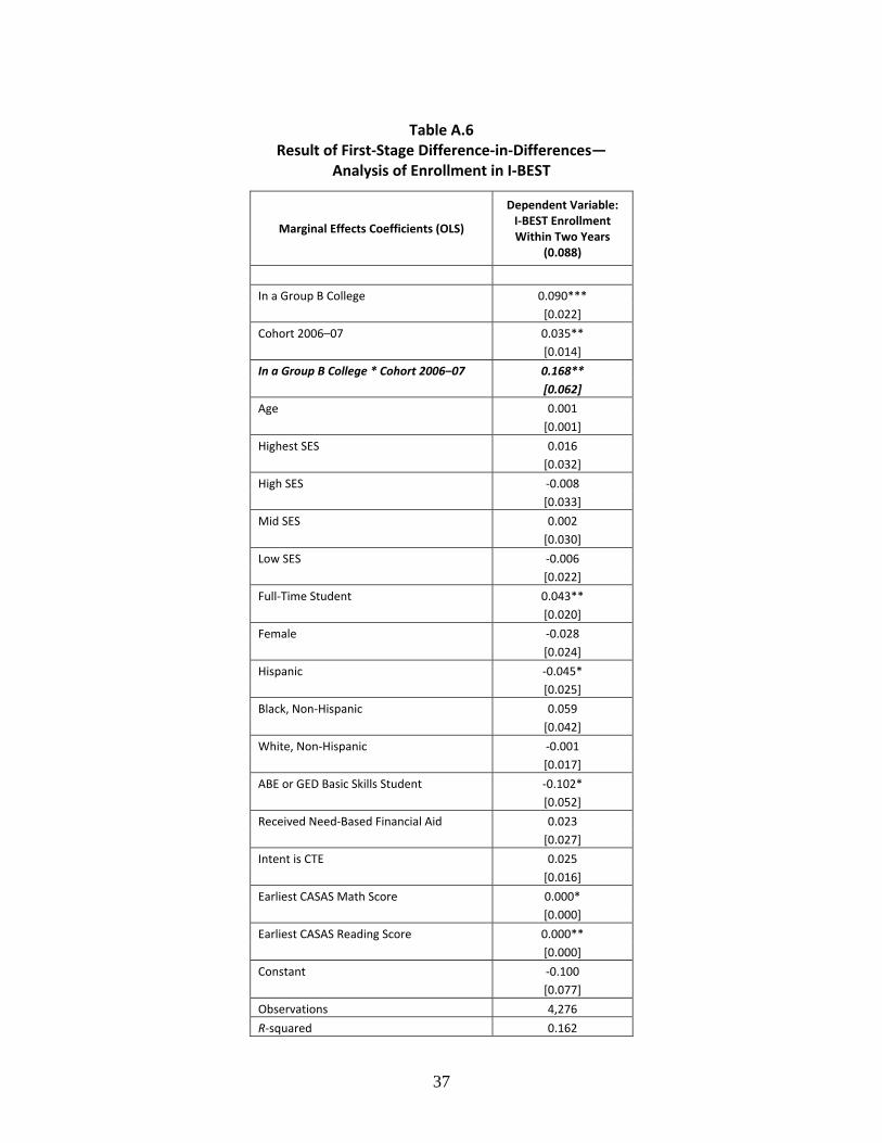
37

 

Table A.6 Result of First‐Stage Difference‐in‐Differences— 

Analysis of Enrollment in I‐BEST  

Marginal Effects Coefficients (OLS) 

Dependent Variable: I‐BEST Enrollment Within Two Years 

(0.088) 

     

In a Group B College  0.090***    [0.022] 

Cohort 2006–07  0.035**    [0.014] 

In a Group B College * Cohort 2006–07  0.168**    [0.062] 

Age  0.001    [0.001] 

Highest SES  0.016    [0.032] 

High SES  ‐0.008    [0.033] 

Mid SES  0.002    [0.030] 

Low SES  ‐0.006    [0.022] 

Full‐Time Student  0.043**    [0.020] 

Female  ‐0.028    [0.024] 

Hispanic  ‐0.045*    [0.025] 

Black, Non‐Hispanic  0.059    [0.042] 

White, Non‐Hispanic  ‐0.001    [0.017] 

ABE or GED Basic Skills Student  ‐0.102*    [0.052] 

Received Need‐Based Financial Aid  0.023    [0.027] 

Intent is CTE  0.025    [0.016] 

Earliest CASAS Math Score  0.000*    [0.000] 

Earliest CASAS Reading Score  0.000**    [0.000] 

Constant  ‐0.100    [0.077] 

Observations  4,276 

R‐squared  0.162 

Appendix B: A Brief Description of Propensity Score Matching

Propensity score matching (PSM) matches “treated” subjects—in this case,

students served by I-BEST programs—to selected untreated “control” subjects—in this

case, basic skills students who did not enroll in I-BEST—who have similar background

characteristics (Rosenbaum & Rubin, 1983; Winship & Morgan, 1999). PSM conducts

comparisons between similar pairs of students who differ on whether or not they received

the treatment but have similar other observed characteristics.

PSM first estimates the “propensity score,” an assessment of the propensity to be

treated, by performing a logit or probit regression of the treatment dummy variable on all

available covariates that, in the researcher’s judgment, have the potential to influence the

chances of being treated. Treated and untreated observations with similar propensity

scores are then matched, and then the average treatment effect on the treated (ATT) can

be estimated; the ATT is the average difference on an outcome of interest between the

matched treated and untreated observations.17 The ATT is the average effect of the

treatment on the sort of person who participates in the program. The effectiveness of

PSM is, in part, a function of having enough relevant information about the cases to

accurately estimate the propensity score in order to accurately estimate the ATT using the

matching process that uses this score.

The matching process selects from those observations for which there is

“common support”, that is, whose distribution of propensity scores are deemed by the

algorithm to be sufficiently close to the propensity scores of the treated observations. The

fact that PSM draws its comparison group from only the observations that give common

support rather than all observations, as is typically done when regression is employed, is

one reason why PSM estimates may be more accurate.

In addition, unlike regression, PSM does not assume a particular functional

relationship between an outcome of interest and the available relevant covariates,

including treatment status. In contrast, if we estimated a linear regression model of an

outcome, such as college credits earned, on a treatment status dummy variable (here I- 17 There are many variants of PSM, many of which match each treated observation to a weighted set of matched untreated observations rather than a single observation. Herein, we have used probit to estimate the propensity score and a local linear regression estimator, which is one method of conducting such a match (Todd, 1999).

38

BEST participation) and a number of controls (such as demographics, etc.), we would

obtain an estimate of a fixed effect of treatment across all of the cases (assuming that we

did not interact the treatment status dummy variable with any other covariates). PSM

does not do this; the treatment effect varies with each matched pair of treated and

untreated cases, and is the difference in the outcome between the two cases.

39

References

Bailey, T., Jenkins, D., & Leinbach, D. T. (2006, September). Is student success labeled institutional failure? Student goals and graduation rates in the accountability debate at community colleges (CCRC Working Paper No.1). New York, NY: Columbia University, Teachers College, Community College Research Center.

Barkley, T., & Davis, B. (2009, April 23). IMF says global recession is deepest since

Great Depression. Wall Street Journal. Retrieved from http://online.wsj.com Belfield, C. & Bailey, T. The Returns and Benefits to Community College: A Review of

the Evidence. Working Paper. New York, NY: Columbia University, Teachers College, Community College Research Center.

Card, D. (1999). The causal effect of education on earnings. In O. Ashenfelter & D. Card

(Eds.), Handbook of Labor Economics (Vol. 3, pp. 1802–1863). Amsterdam, Netherlands: Elsevier.

Crosta, P. M., Leinbach, T., & Jenkins, D. (with Prince, D., & Whittaker, D.) (2006,

July). Using census data to classify community college students by socioeconomic status and community characteristics (CCRC Research Tools No. 1). New York, NY: Columbia University, Teachers College, Community College Research Center.

Dynarski, S. M. (2000). Hope for whom? Financial aid for the middle class and its impact

on college attendance. National Tax Journal, 53(3), 629–662.

Grubb, W.N. (2002). Learning and earning in the middle, Part II: state and local studies of pre-baccalaureate education. Economics of Education Review, 21, 401-414.

Heckman, J. J., & Smith, J. A. (1999, July). The pre-programme earnings dip and the

determinants of participant in a social programme: Implications for simple programme evaluation strategies. The Economic Journal, 109(457), 313–348.

Jacobson, L., & Mokher, C. (2009, January). Pathways to boosting the earnings of low-

income students by increasing their educational attainment. The Hudson Institute and CNA.

Jenkins, D., Zeidenberg, M., & Kienzl, G. S. (2009). Educational outcomes of I-BEST,

Washington State Community and Technical College System’s Integrated Basic Education and Skills Training Program: Findings from a multivariate analysis (CCRC Working Paper No.16). New York, NY: Columbia University, Teachers College, Community College Research Center.

Kennedy, P. (2003). A guide to econometrics. Cambridge, MA: MIT Press.

40

41

Prince, D., & Jenkins, D. (2005, April). Building pathways to success for low-skill adult students: Lessons for community college policy and practice from a longitudinal student tracking study (CCRC Brief No. 25). New York, NY: Columbia University, Teachers College, Community College Research Center.

Puma, M. J., Olsen, R. B., Bell, S. H., & Price, C. (2009, October). What to do when data

are missing in group randomized controlled trials (NCEE Report No. 2009-0049). Washington, DC: U.S. Department of Education, Institute of Education Sciences, National Center for Education Evaluation and Regional Assistance. Retrieved from http://ies.ed.gov/ncee/pdf/20090049.pdf

Rosenbaum, P. R., & Rubin, D. B. (1983). The central role of the propensity score in

observational studies for causal effects. Biometrika, 70(1), 41–55. Todd, P. E. (1999). A practical guide to implementing matching estimators. Philadelphia,

PA: Department of Economics, University of Pennsylvania. Retrieved from http://athena.sas.upenn.edu/~petra/papers/prac.pdf

U.S. Department of Education, Office of Vocational and Adult Education. (2007). Adult

Education Annual Report to Congress Year 2004–05, Washington, DC: Author. Retrieved from www.ed.gov/offices/OVAE

Wachen, J., Jenkins, D., and Van Noy, M. (with Kulongoski, K., Kurien, K., Richards,

A., Sipes, L., Weiss, M., and Zeidenberg, M.) (2010). How I-BEST works: Findings from a field study. New York, NY: Columbia University, Teachers College, Community College Research Center.

Washington State Board for Community and Technical Colleges (2006). The

socioeconomic well-being of Washington State: Who attends community and technical college. Olympia, WA: Author. Retrieved from http://www.sbctc.ctc.edu/docs/data/research_reports/resh_06-4_socioeconstudy.pdf

Winship, C., & Morgan, S. L. (1999). The estimation of causal effects from observational

data. Annual Review of Sociology, 25, 659–707.