Waiting Time Distributions for IP3 gated Ca2+

Channels

Diplomarbeitam Fachgebiet Physik

Institut für Theoretische PhysikFreie Universität Berlin

vorgelegt vonHeiko SchmidleOktober 2008

Betreuer: PD Dr. Martin Falcke

Heiko SchmidleWrangelstr. 5410997 Berlin

II

Contents

List of Figures V

1 Introduction 1

2 Fundamentals 72.1 Biological Basics . . . . . . . . . . . . . . . . . . . . . . . . . . . . . . . 7

2.1.1 Cell Signaling . . . . . . . . . . . . . . . . . . . . . . . . . . . . . 72.1.2 Intracellular Signal Transduction . . . . . . . . . . . . . . . . . . 72.1.3 Ion Transport . . . . . . . . . . . . . . . . . . . . . . . . . . . . . 92.1.4 Experiments . . . . . . . . . . . . . . . . . . . . . . . . . . . . . . 92.1.5 Ca2+ Channel Models . . . . . . . . . . . . . . . . . . . . . . . . 13

2.2 Mathematical Methods . . . . . . . . . . . . . . . . . . . . . . . . . . . . 172.2.1 Stochastic Processes . . . . . . . . . . . . . . . . . . . . . . . . . 172.2.2 The Master Equation . . . . . . . . . . . . . . . . . . . . . . . . . 182.2.3 Properties . . . . . . . . . . . . . . . . . . . . . . . . . . . . . . . 202.2.4 Reduction Methods . . . . . . . . . . . . . . . . . . . . . . . . . . 242.2.5 Gillespie Simulation . . . . . . . . . . . . . . . . . . . . . . . . . . 28

2.3 Numerical Methods . . . . . . . . . . . . . . . . . . . . . . . . . . . . . . 302.3.1 Matrix Transformations . . . . . . . . . . . . . . . . . . . . . . . 312.3.2 Eigenvalues and Eigenvectors . . . . . . . . . . . . . . . . . . . . 33

3 Waiting Time Distribution and Results 353.1 Opening Time Distribution . . . . . . . . . . . . . . . . . . . . . . . . . . 35

3.1.1 Single Channel Activation . . . . . . . . . . . . . . . . . . . . . . 353.1.2 Cluster Activation . . . . . . . . . . . . . . . . . . . . . . . . . . 38

3.2 Closing Time Distribution . . . . . . . . . . . . . . . . . . . . . . . . . . 39

III

Contents

3.2.1 Construction of the Cluster State Matrix . . . . . . . . . . . . . . 393.2.2 Initial Probabilities . . . . . . . . . . . . . . . . . . . . . . . . . . 403.2.3 First Closing Time . . . . . . . . . . . . . . . . . . . . . . . . . . 413.2.4 Reduction of the Channel State Transition Matrix . . . . . . . . . 413.2.5 Comparison of di�erent Reduction Methods . . . . . . . . . . . . 453.2.6 Cross Correlations . . . . . . . . . . . . . . . . . . . . . . . . . . 46

3.3 Computational Results . . . . . . . . . . . . . . . . . . . . . . . . . . . . 483.3.1 Opening Time . . . . . . . . . . . . . . . . . . . . . . . . . . . . . 503.3.2 Closing Time . . . . . . . . . . . . . . . . . . . . . . . . . . . . . 523.3.3 Criteria for Reduction . . . . . . . . . . . . . . . . . . . . . . . . 593.3.4 Cross Correlations . . . . . . . . . . . . . . . . . . . . . . . . . . 62

4 Discussion and Outlook 63

A Parameter Values VII

B Proofs IXB.1 Proof of Existence of Long Time Limit . . . . . . . . . . . . . . . . . . . IXB.2 Proof of Detailed Balance . . . . . . . . . . . . . . . . . . . . . . . . . . XI

C Perron Cluster XIII

D Aggregate States Composition XV

Bibliography XIX

IV

List of Figures

1.1 Global Ca2+ release in oocytes and eggs . . . . . . . . . . . . . . . . . . 3

2.1 Ca2+ signaling pathway . . . . . . . . . . . . . . . . . . . . . . . . . . . . 82.2 Experimental results by Parker and Yao . . . . . . . . . . . . . . . . . . 102.3 Experimental results Machaca . . . . . . . . . . . . . . . . . . . . . . . . 112.4 Experimental results Sun et al. in 3 dim. plots . . . . . . . . . . . . . . . 122.5 Electron microscope picture of calcium channel . . . . . . . . . . . . . . 142.6 Subunit model 1 . . . . . . . . . . . . . . . . . . . . . . . . . . . . . . . 152.7 Subunit model 3 . . . . . . . . . . . . . . . . . . . . . . . . . . . . . . . 16

3.1 Reduction methods applied to the 13 states model . . . . . . . . . . . . . 463.2 Expected opening time . . . . . . . . . . . . . . . . . . . . . . . . . . . . 493.3 Opening time distribution of all three models . . . . . . . . . . . . . . . 513.4 Expected closing time . . . . . . . . . . . . . . . . . . . . . . . . . . . . 523.5 Closing time distributions of all three models . . . . . . . . . . . . . . . . 533.6 Logarithmic plots of opening and closing time . . . . . . . . . . . . . . . 553.7 Number of inhibited states and closing time distribution for �xed and

variable Ca2+ concentration . . . . . . . . . . . . . . . . . . . . . . . . . 563.8 Analytic and simulation results . . . . . . . . . . . . . . . . . . . . . . . 583.9 Results for a various number of aggregate states . . . . . . . . . . . . . . 593.10 Expected closing time as function of the number of channels . . . . . . . 603.11 Expected closing time and number of open aggregate states for 2 channels

in model 1 . . . . . . . . . . . . . . . . . . . . . . . . . . . . . . . . . . . 613.12 Cross correlation of model 1 . . . . . . . . . . . . . . . . . . . . . . . . . 62

4.1 Computation time for opening and closing time . . . . . . . . . . . . . . 64

V

List of Figures

C.1 Perron cluster of all three models . . . . . . . . . . . . . . . . . . . . . . XIII

VI

1 Introduction

With a huge gain in experimental skills, biologists are now capable to study activitiesin living systems on a molecular level. This caused the formation of a new disciplinein science, the molecular biology. Molecular biology touches �elds of classical physics.Borders between both disciplines begin to disappear and they can learn from each other.Physicist use known concepts to study problems for example in neuronal systems, nu-trients networks and cell signaling.

In this diploma thesis my focus lies on a cell signaling mechanism. In some wordsmy aim is to determine the opening and closing probability distribution of ion channelswhich exist within living cells.

'Almost everything we do is controlled by Ca2+- how we move, how our heart beatsand how our brain stores information'. This citation from a famous paper by Berridgeet al. in Nature [8] demonstrates the necessity to understand calcium signaling in cells,they called Ca2+ even 'a life and death signal'.

Ca2+ plays an important role as intercellular as well as intracellular messenger. Itcan pass through ion channels in the plasma membrane, the cell border, or within the cellthrough the ER membrane. The ER is a storage compartment in cells which performsmany di�erent cellular functions. Both levels of calcium spread can be observed e.g.in smooth muscles, Ca2+ signals within the cell cause muscle relaxation but signalsbetween cells cause muscle contraction [3]. Cells can interpret modest changes in theconcentration of Ca2+, for example di�erent genes can be activated by changing theamplitude of Ca2+ signals and they control in embryos splitting of groups of cells toperform specialized functions. Ca2+ signaling helps in amphibia or in zebra�sh to specifywhat cells form which part of the body [8]. In fertilization processes Ca2+ waves appear,as shown Fig. 1.1, what have been the �rst Ca2+ waves observed [19]. Ca2+ is alsoinvolved in development of the nervous system, to slow down the growth of certain

1

1 Introduction

aggressive cancer cells and in the proliferation of immune cells [8]. Ca2+ contributes ina very important way to the activity of neurons, since the spatial and temporal patternof Ca2+ has an impact in stimulating or depressing the transmission of neuron signals[9].

This short journey through Ca2+ signaling in cells shows the universality of thesignaling mechanism. Therefore it is very important to study and to understand howCa2+ controls processes in living systems.

But how can Ca2+ act as a signaling mechansism, since it is just a simple ion? Forinstance information can be spread via spatial and temporal patterns of calcium concen-tration within or between cells. The concentration patterns are in general produced bytwo classes of ion transport proteins: ion pumps and ion channels. Ion pumps transportions through cell or Endoplasmatic Reticulum (ER) membranes against their concen-tration gradient. The energy they need is supplied by Adenosine Triphosphate (ATP),which acts as a carrier of chemical energy [3]. Ion channels, on the other hand, are poresin membranes and open or close due to stochastic binding of signaling molecules. Theylet ions pass in direction of the concentration gradient and thus no energy is needed.

I am particularly interested in the ion channels. Ca2+ channels are proteins in themembrane, which open due to a stochastic binding of signaling molecules to bindingsites. A channel type present in the ER membrane of many cells is the Inositol 1,4,5-Trisposphate (IP3) receptor channel. Our interest in this work is focussed on this type ofCa2+ channels. The open probability depends on the Ca2+ and IP3 concentration in thecell since channels open due to a binding of Ca2+ and IP3 to receptors. The channels aregrouped together in clusters and the clusters are randomly distributed on the ER mem-brane [19]. The release of calcium by one channel is a stochastic event, which increasesthe Ca2+ concentration in its environment. This e�ect raises the open probability of itsneighbors and thus the release is a self amplifying mechanism, called CICR (CalciumInduced Calcium Release). To regulate the release, the closing probability depends onthe Ca2+ concentration as well, therefore high concentrations of Ca2+ inhibit the chan-nel and lead to its closure. These Ca2+ and IP3 dependent probabilities show nonlinearbehavior. Calcium dynamics in cells are thus determined by two characteristics, chanceand nonlinearity.

Through this mechanism, Ca2+ channels have the possibility to communicate and

2

1 Introduction

Figure 1.1: Global Ca2+ wave in oocytes and eggs recorded by Machaca et al.[28]. Bluerepresents a low Ca2+ concentration and red very high. In the lower panels time isindicated in seconds.

to build a huge variety of signals. They can be divided in three di�erent types: asingle calcium channel releases calcium and closes directly, called a blip. Secondly,the opening provokes release of neighbored channels and thus a cluster opens, called apu�. The third pattern is a release event that spreads over the whole cell leading to acalcium wave. Furthermore, the self regulating mechanism (CICR) leads to oscillationsof calcium concentration. Channels open and close in regular time intervals controlled bythe concentration. All these di�erent kinds of Ca2+ releases allow an enormous variationof calcium signals, which are used to transport information in living systems. In thiswork we are interested in Ca2+ pu�s of a cluster of channels.

We will not study the whole signaling pathway of calcium since this would go beyondthe scope of this diploma thesis. Activated by a signaling molecule outside the cell, a G-protein is activated which leads to a raises the concentration of a second messenger, whichare signaling molecules within a cell. Binding of this messenger to calcium channels cancause an opening of the channel in the ER membrane and thus the Ca2+ concentrationin the cytosol raises rapidly. The cytosol is the liquid that �lls the cell. It consists ofwater with many di�erent dissociated ions, proteins and other molecules what makes itlike a gel.

At this point I start the work, since I am interested in the probability density distri-bution until one cluster of several channels opens (Opening Time) and afterwards thetime of its closure (Closing Time).

Calcium signaling and calcium oscillations have been investigated for 20 years bynow. Many di�erent approaches and models have been developed. Early approaches de-scribe Ca2+ dynamics by ordinary di�erential equations of �uxes. Fluxes are determined

3

1 Introduction

by multiple channels, pumps and exchangers [48]. Oscillations can be explained by afeedback loop and cooperativity [29]. The whole cell was considered as a homogenousmedium. Experimental progress led to the development of new concepts, that accountedfor inhomogeneity in cells. Local cell dynamics were studied in terms of partial di�eren-tial equations. These models focus on the kinetics of single channels [35, 48] but neglect�uctuations. Based on the model, �ux balance equations can be constructed and thedependencies of the �ux rates on the model variables must be speci�ed [35]. Thesemodels were able to describe Ca2+ oscillation, which were caused by a Hopf Bifurcationof di�erential equations describing the dynamics. These concepts are hard to extend tothe whole cell level, because the equations are very complex and di�cult to compute.

New experimental �ndings revealed the stochastic character even of global Ca2+

release events [30, 40]. These results are con�rmed by theoretical results, that show thatCa2+ dynamics are determined by �uctuations of molecules [46]. Ca2+ dynamics canno longer be described by deterministic models, but by stochastic cell models. Randombinding of signaling molecules to Ca2+ channels seem to evoke even Ca2+ waves andoscillations in cells and are thus not negligible [18, 17, 40]. Stochastic models existalready for subunits and channels, but now they can be extended to cluster and celllevel. The new approach is able to explain the hierarchical structure of Ca2+ signals,blips, pu�s and waves and to explain oscillations in the whole cell. The low number ofchannels and clusters guarantees stochastic behavior. The system of ion channels in cellsis a seldom observable stochastic process in nature. Experimenters are able to measuresingle channel activities and to provide a real insight into a stochastic process. With thisnew approach, cell models can be developed that account for local stochastic behavior.Therefore, local dynamics have to be studied in detail to build the basis of extensionsto cell models.

The aim of this diploma thesis is to use the stochastic character of local calciumrelease and to �nd an expression in matrix terms of the cluster dynamics and hence toformulate the problem in Master Equation formalism. Afterwards, I determine waitingtime distributions, i.e. the opening and closing probability distribution of one cluster bysolving the Master Equation. Then I use this formalism to study qualities of di�erentmodels, that have been developed to explain channel and cluster behavior.

The �rst part of the diploma thesis gives a brief introduction into the basic concepts

4

1 Introduction

to understand cell signaling and the calcium pathway in general. Then I introduce themathematical basis to treat the problem of waiting time distributions for calcium chan-nels. Stochastic processes, Markov processes and the most important properties of thisprocesses are key words of that section. Then, I will turn towards the actual problem,the waiting time distributions of the opening and closing time of Ca2+ channels. I showhow the concrete problem can be formulated in terms of our theoretical framework andhow we can �nd a solution. A problem appears at this point, namely the states matrixwe use to compute the closing time is much too large in dimensions. Therefore I willdemonstrate how we developed a robust and fast reduction method to overcome thisproblem. Afterwards I will apply our method to three di�erent models that describecalcium channels in a di�erent manner and are of fundamental interest [2, 41, 50]. Dif-ferences of them will be worked out and I evaluate their capacity to describe calciumchannels, by comparing the analytic results to stochastic simulations [22]. Moreover, Itry to analyse our reduction method, by studying di�erent details. The last point in thisdiploma thesis will be a discussion of the results we obtained and a brief comparisonwith experiments.

5

1 Introduction

6

2 Fundamentals

2.1 Biological Basics

2.1.1 Cell SignalingCells need to communicate. They are the components of living systems which ful�lldistinct functions. Thus they have to exchange information, whereas many di�erentways exist. In general, signaling molecules are synthesized and released by signalingcells. Signaling molecules are then transported through the living system and producea speci�c response only in target cells. Target cells have special receptors to decode theinformation [16]. Most of receptors are activated by binding of growth factors, neuro-transmitters, pheromones, etc. Others are activated by changes in the concentration ofa metabolite, e.g. oxygen or nutrients or by physical stimuli like light, touch or heat.After a signaling molecule has produced a speci�c response in a cell, the removal of thesignal follows. Changes in concentration should be reversed since communication is notone single process but a continuous exchange.

In this work my focus is on signaling from a group of receptor proteins located inthe plasma membrane of a cell. The signaling molecule outside the cell acts as a ligandwhich binds to a complementary site on the extracellular domain of the receptor. Thebiding initiates a signaling pathway in the cytosol, including an intracellular messenger.This intracellular messenger itself causes Ca2+ release in the cell from the ER to thecytosol via Ca2+ channels.

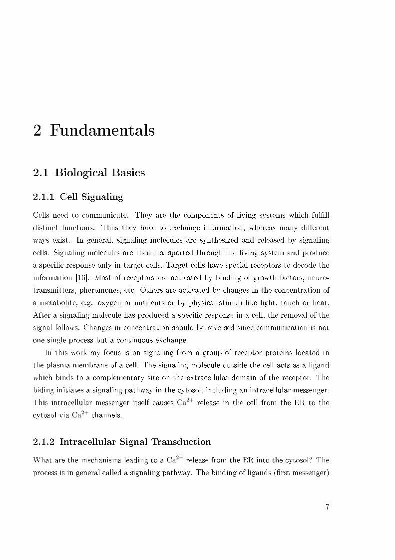
2.1.2 Intracellular Signal TransductionWhat are the mechanisms leading to a Ca2+ release from the ER into the cytosol? Theprocess is in general called a signaling pathway. The binding of ligands (�rst messenger)

7

2 Fundamentals

Figure 2.1: Illustration of the Ca2+ pathway, table from [1]. After a signal molecule (lig-and) activates the G-protein it activates the enzyme phospholipase C which catalyzesthe reaction of PIP2 to IP3 in the cel membrane. The increase of IP3 concentrationin the cytosol leads to an higher probability of the calcium channel to open in the ERmembrane, what leads to a cellular response.

to receptors, which are transported through the living system like a human body byblood circuit, lead to a short lived increase in the concentration of certain low molecularweight intracellular signaling molecules (second messenger). There exists a variety ofsecond messengers, but we are interested in IP3, because it is the most important secondmessenger and responsible for calcium release from the ER into the cytosol. The signal-ing pathway of a calcium release event starts at the extracellular receptor protein. Twofamilies of these receptors exist, the G-protein coupled receptors and the Tyrosine-kinasereceptors. Stimulation of the receptor by a ligand causes activation of the G-protein,which in turn modulates the activity of an associated e�ector protein. All e�ector pro-teins are either membrane bound ion channels or enzymes, that catalyze the formationof second messengers. In this pathway the G-protein is activated, which activates itselfthe enzyme Phospholipase C. The enzyme catalysis the reaction of PhosphatidylinositolBisphosphate (PIP2) to IP3 in the cell membrane, which leads to an increase of the IP3

concentration in the cytosol [16] and consequently to a raise of the open probability

8

2 Fundamentals

of IP3 gated Ca2+ channels in the ER membrane. This is a protein, composed of fouridentical subunits, each containing an IP3 binding site.

The processes that lead to an opening of the channel are discussed in further detail inSec. 2.1.5. The pathway is illustrated in Fig. 2.1. Calcium release induces downstreamsignaling pathway leading, for example, to a modi�cation of gene expression or musclecontraction. At high concentrations it inhibits the IP3 gated channels and they close.The ATPase pumps located in the plasma membrane and ER membrane constantlypump Ca2+ from the cytosol outside the cell or back into the ER. Without some meansof replenishing depleted stores of intracellular Ca2+ a cell would soon be unable todecrease the cytosolic Ca2+ level. High calcium concentration can even be lethal forcells.

2.1.3 Ion TransportAs mentioned in Chapter 1, two main classes of ion transport proteins in cells exist.ATP powered ion pumps and ion channels, which are pores that allow di�erent ions(Na+, K+, Ca2+, CL−) to move through membranes down their concentration gradient.We can di�er between three groups of ion channels, Voltage Operated Channels, Re-ceptor Operated Channels and Store Operated channels [9]. Concentration gradientsand selective movement of ions through channels constitute the principle mechanism bywhich a di�erent voltage, or electric potential, is generated across the plasma membrane,which is responsible for the opening of channels. The second kind are ion channels thatopen in response to receptor activation, like ligands or second messengers. Binding ofmessenger molecules to channel proteins cause an opening of the channel and ions canpass through. A third class of channels can be found in the plasma membrane, thestore operated channels, which open due to signals generated by store emptying. Thismechanism is not yet understood very well [9].

2.1.4 ExperimentsWe are interested in experiments that study local Ca2+ release events of some channels,i.e. a cluster, in the ER membrane within a cell. In general it is di�cult to access Ca2+

concentration in cells, however during the last years experimenters developed advanced

9

2 Fundamentals

A B

C

Figure 2.2: (A) Pu�s and waves of an oocyte, evoked by increasing photorelease of IP3.The �ash duration is indicated on the left side next to the plot. (B) Blip (noisy trace)and pu� (smooth trace), both rise times are similar.(C) Results for di�erent pu�s areshown. In all plots the y-axis is the ratio of the �uorescence signal ∆F/F.

methods. I do not explain experimental details, since this would go far beyond thescope of this work and they can be found in corresponding articles. Experimentersuse a �uorescence signal, that depends on the Ca2+ concentration, which is recordedby light sensitive cameras. Spatial and temporal changes in the Ca2+ concentrationcan be recorded. ∆F/F is the relative amount of total released Ca2+ recorded by the�uorescence signal. One of the �rst experiments that recorded single Ca2+ release eventswas made by Parker and Yao in 1996 [30]. They a�rmed three classes of release events,blips, pu�s and waves, see Fig. 2.2 A. Since we compute the waiting time distributionof a cluster of channels, we are interested in the pu� dynamics. Fig. 2.2 shows di�erent

10

2 Fundamentals

A B

Figure 2.3: (A) Average time course of Ca2+ pu� release from oocyte (squares) andegg (circles). (B) Same experiment as A for a single release event (blip). Plots showthe ratio of the �uorescence signal ∆F/F0.

results for pu�s in oocyte cells. We notice that blips and pu�s have comparable timescales, see Fig. 2.2 B. Time scales for such events are some hundred milliseconds, whereasthe maximum is after approximately 100 ms. The parameter values of the channel modeldeveloped by Sneyd et al. [41], see Sec. 2.1.5, were �tted to this results.

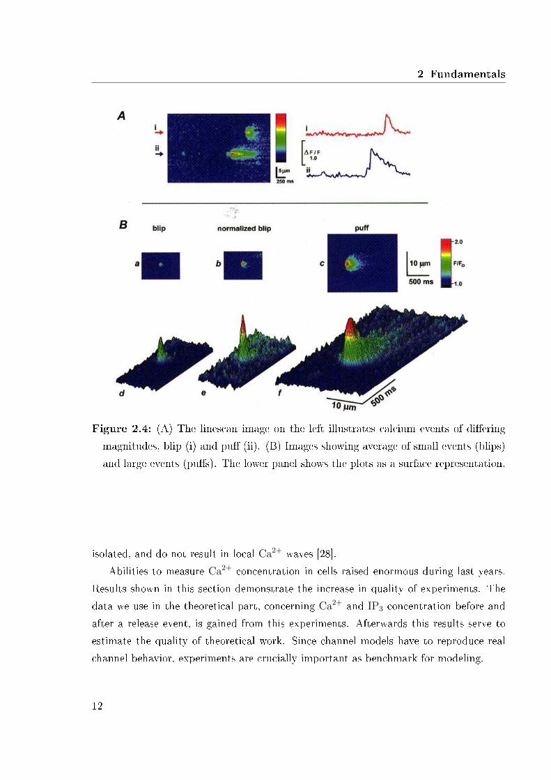
In 1998 Sun et al. [44] con�rmed the results of Parker et al. Experiments were alsodone with oocytes by using the same experimental methods than Parker et al. Resultsreveal the same time scale and behavior of calcium release, but also a wide range oftime scales for calcium pu�s between 100 − 600 ms. Images in Fig. 2.4 were obtainedby averaging selected blips (n=5) and pu�s (n=4) after aligning the original images inspace and time relative to the peak �uorescence signal in each case [44]. Plots in Fig. 2.4show the large Ca2+ gradient after a release event of blips and pu�s. In Fig. 2.4 (B)three dimensional plots show clearly the di�erences between blips and pu�s.

Machaca studied 2004 two groups of Xenopus oocytes, one group was untreated(oocytes) and the second matured (eggs). Although discrete Ca2+ release events canbe resolved, they vary in their spatial and temporal kinetics. These elementary releaseevents were divided into two groups: Ca2+ pu�s refer to the smallest release event andsingle release event refer to larger Ca2+ release events that are still discrete, spatially

11

2 Fundamentals

Figure 2.4: (A) The linescan image on the left illustrates calcium events of di�eringmagnitudes, blip (i) and pu� (ii). (B) Images showing average of small events (blips)and large events (pu�s). The lower panel shows the plots as a surface representation.

isolated, and do not result in local Ca2+ waves [28].Abilities to measure Ca2+ concentration in cells raised enormous during last years.

Results shown in this section demonstrate the increase in quality of experiments. Thedata we use in the theoretical part, concerning Ca2+ and IP3 concentration before andafter a release event, is gained from this experiments. Afterwards this results serve toestimate the quality of theoretical work. Since channel models have to reproduce realchannel behavior, experiments are crucially important as benchmark for modeling.

12

2 Fundamentals

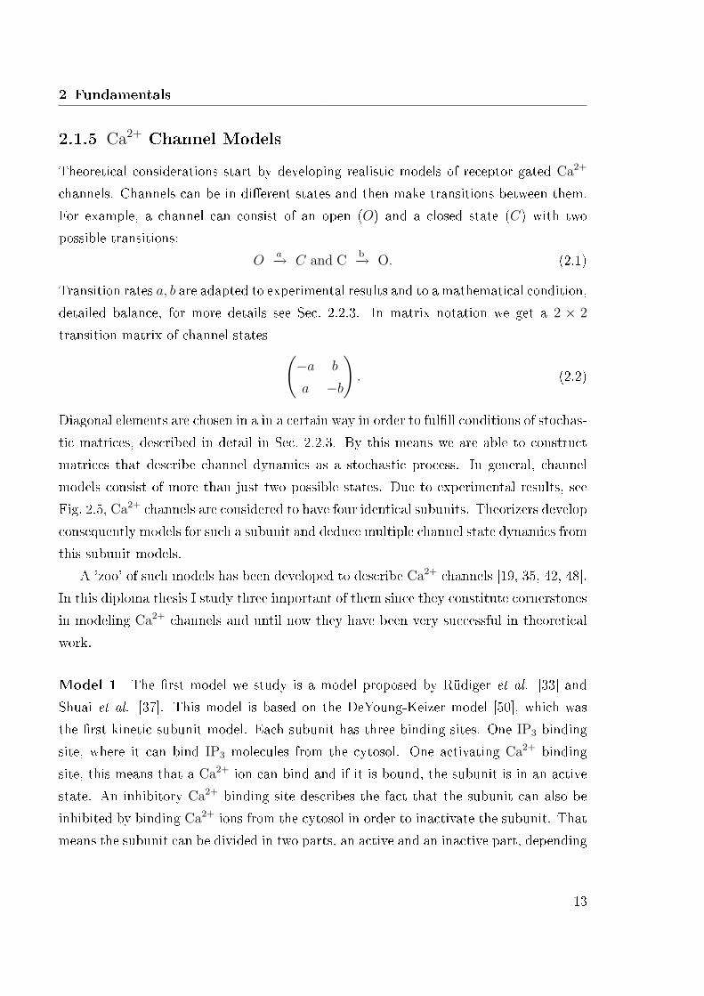
2.1.5 Ca2+ Channel ModelsTheoretical considerations start by developing realistic models of receptor gated Ca2+

channels. Channels can be in di�erent states and then make transitions between them.For example, a channel can consist of an open (O) and a closed state (C) with twopossible transitions:

Oa−→ C and C

b−→ O. (2.1)

Transition rates a, b are adapted to experimental results and to a mathematical condition,detailed balance, for more details see Sec. 2.2.3. In matrix notation we get a 2 × 2

transition matrix of channel states(−a b

a −b

). (2.2)

Diagonal elements are chosen in a in a certain way in order to ful�ll conditions of stochas-tic matrices, described in detail in Sec. 2.2.3. By this means we are able to constructmatrices that describe channel dynamics as a stochastic process. In general, channelmodels consist of more than just two possible states. Due to experimental results, seeFig. 2.5, Ca2+ channels are considered to have four identical subunits. Theorizers developconsequently models for such a subunit and deduce multiple channel state dynamics fromthis subunit models.

A 'zoo' of such models has been developed to describe Ca2+ channels [19, 35, 42, 48].In this diploma thesis I study three important of them since they constitute cornerstonesin modeling Ca2+ channels and until now they have been very successful in theoreticalwork.

Model 1 The �rst model we study is a model proposed by Rüdiger et al. [33] andShuai et al. [37]. This model is based on the DeYoung-Keizer model [50], which wasthe �rst kinetic subunit model. Each subunit has three binding sites. One IP3 bindingsite, where it can bind IP3 molecules from the cytosol. One activating Ca2+ bindingsite, this means that a Ca2+ ion can bind and if it is bound, the subunit is in an activestate. An inhibitory Ca2+ binding site describes the fact that the subunit can also beinhibited by binding Ca2+ ions from the cytosol in order to inactivate the subunit. Thatmeans the subunit can be divided in two parts, an active and an inactive part, depending

13

2 Fundamentals

Figure 2.5: Electron-Microscope picture of a Ca2+ channel protein by Jiang et al. [26].Four identical subunits can be identi�ed.

on whether Ca2+ or IP3 is bound to an active or inactive binding site. De Young andKeizer developed this model in answer to new experimental results. They used it inthermodynamic limit as a deterministic model, but we will construct a stochastic matrixbased on the model.

Subunit states are represented by a triplet (ijk), where i, j and k represent these threebinding sites respectively. An occupied site is represented by an 1 and an unoccupied bya 0. In this model the subunit is considered to be in an active state when it is in state(110) [50]. That is, when the IP3 and activating Ca2+ binding sites are occupied butthe inhibitory Ca2+ site is unoccupied. All possible combinations result in eight subunitstates. Rüdiger et al. [33] added an extra state labeled 'Active' with transitions to andfrom state (110) in order to get better agreement with experimental data. The subunitis only active when it is in this state. In this work, we have combined the 'Active'state and state (110) to one single state by assuming the transition rates between thetwo states are fast, and so reduced the nine state model to eight states. In Sec. 2.2.4we will see, that it is very important to minimize the maximum number of states forreasons of computationally costs. Probabilities to bind Ca2+ and IP3 are involved in thetransition rates between all possible subunit states. Model 1 is illustrated in Fig. 2.6,with transition rates ai, bi, c and p indicate the Ca2+ and IP3 concentration, respectively.We use the transition rates given in [37] (see Tab. A.1 in the Appendix with Ki = bi/ai).As aforementioned a channel consists of four identical subunits and we consider a channel

14

2 Fundamentals

b0

a0

b1

a1p

b2

a2c

b3a3p

b4

a4c

b5

a5c

Active

110 111

011010

101

001000

100

a2c

b2

b4

a4c

b1

a1p

b3a3p

b5

a5c

b5

a5c

b5

a5c

Unbound Bound

Unbound

Bound

Unbound

Bound

IP3

Inhibitory Ca2+

Act

ivat

ion C

a2+

Figure 2.6: Subunit model from DeYoung-Keizer, [50] extended by one state fromRüdiger et al. [33]. The ai's and bi's are transition rates, c and p are the Ca2+ andIP3 concentration in the cytosol.

as open when any three of the four subunits are in an active state.

Model 2 Adkins and Taylor [2] suggested that the binding of Ca2+ to the activatingand inhibitory binding sites may be a�ected whether the IP3 binding site is occupied ornot. They propose that if IP3 is bound, then Ca2+ cannot bind to the inhibitory Ca2+

binding site, and if IP3 is not bound, then Ca2+ cannot bind to the activating bindingsite. That means model 2 is the same scheme as model 1, but the activating Ca2+

binding rate when IP3 is not bound and the inhibitory Ca2+ binding rate when IP3 isbound are made small. We set them to 1.0× 10−3 µM−1s−1, what is small compared toresting transition rates (compare Tab. A.1 in the Appendix). We have to pay attentionto the detailed balance condition and thus we set the corresponding reverse transitionrates also small, so that the dissociation constants Ki = bi/ai remain the same. This isdemonstrated in Fig. 2.6 by dashed lines for the transitions we make slow.

15

2 Fundamentals

Figure 2.7: (A) Scheme of subunit model 3 by Sneyd and Dufour [41]. (B) Triangularmotifs replaced by square motifs by Falcke [19]. R′, R, R represent receptor states,I1, I1 inhibited states, O′, O, O open states, A, A activated states, I2, I2 inactive statesand S the shut state. c and p are the Ca2+ and IP3 concentration, respectively.

Model 3 Sneyd and Dufour [41] propose a 10 states model for the subunits of theCa2+ channel. This model includes one IP3 binding site, two binding sites for Ca2+

activation and one binding site for Ca2+ inactivation. The structure of this model isthat the receptor R can bind Ca2+ and inactivate to state I1 or it can bind IP3 andopen to state O. State O can then shut to state S or bind Ca2+ and activate to stateA. State A can then bind Ca2+ and inactivate to state I2. The division of these statesin multiple understates, e.g. R in R, R′, R is designed to produce agreement with anumber of results from experimental data. Falcke [19] suggested a way to overcome aproblem involving a lack of Ca2+ conservation in triangular motifs of this model, seeright hand side of Fig. 2.7. That is, in a cyclic transition from R → R′ → I2 → R onewould pick up a Ca2+ ion and in the other direction one would loose an ion. The sameproblem exists for the other triangular motifs. Falcke proposed three additional statesand replaced the triangular by square motifs, see left hand side Fig. 2.7. The wholemodel is a combination of 2.7 (A) and (B), that results in 13 subunit states. We useparameter values given in [41], but we change them slightly in order to ful�ll detailedbalance for the system, see Tab. A.2. A channel consists of four identical subunits andwe consider the channel as open when all four subunits are in states O′, O, O (open

16

2 Fundamentals

states) or in states A, A (activate states) or an intermediate combination of these �vestates.

2.2 Mathematical MethodsThe fundamental concepts needed for this work are stochastic processes and the spe-cial case of Markov processes. I derive the fundamental Master Equation from theChapman-Kolmogorov Equation and then I prove some important properties of theMaster Equation. In this chapter I follow textbooks van Kampen [27] and Gardiner[12].

2.2.1 Stochastic ProcessesStochastic processes are systems that evolve probabilistically in time or systems in whicha certain time dependent random variable X(t) exists. We can measure the valuesx1, x2, x3, . . . of X(t) at t1, t2, t3, . . . and we assume that a set of joint probability densities,p(x1, t1; x2, t2; x3, t3; . . .), exists, which describe the system completely. With these jointprobability density functions, I can also de�ne a conditional probability density for astochastic process

p(x1, t1; x2, t2; . . . |y1, τ1; y2, τ2; . . .)

= p(x1, t1; x2, t2; . . . ; y1, τ1; y2, τ2; . . .)/p(y1, τ1; y2, τ2; . . .).(2.3)

This is valid independently of the ordering of the times, but it is common to consideronly times which increase t1 ≤ t2 ≤ t3 ≤ . . ..

The de�nition of a stochastic process is very loose, but to de�ne one such processone has to know at least all joint probabilities of the kind above. The simplest case arecompletely separable stochastic processes

p(x1, t1; x2, t2; . . .) =∏

i

p(xi, ti). (2.4)

I consider now the next simple case of stochastic processes, the Markov processes. Theconditional probability density is determined entirely by the knowledge of the most recentvalue, i.e. the process has no memory. For a set of successive times t1 < t2 < . . . < tn

17

2 Fundamentals

one has

p1,n−1(xn, tn|x1, t1; x2, t2; . . . ; xn−1, tn−1) = p1,1(xn, tn|xn−1, tn−1). (2.5)

That is, the conditional probability at time tn, given the value xn−1 at tn−1 is uniquelydetermined and is not a�ected by any knowledge of the values at earlier times. pn,m iscalled the transition probability. A Markov process is fully determined by p1(x1, t1) andp1,1(x2, t2|x1, t1), because the whole hierarchy can be constructed from them

p3(x1, t1; x2, t2; x3, t3) = p2(x1, t1; x2, t2)p1,2(x3, t3|x1, t1; x2, t2)

= p1(x1, t1)p1,1(x2, t2|x1, t1)p1,1(x3, t3|x2, t2).(2.6)

Continuing this algorithm one can �nd successively all p's. This property makes theMarkov processes manageable and explains why this processes are so useful. One fa-mous example is brownian motion. A heavy particle is in a �uid of light molecules,which collides with the molecules in a random fashion. The dissociation of gas of bi-nary molecules is also markovian. A molecule has a certain probability to break up bycollisions with heavy gas molecules.

If a certain physical process is not markovian, it is sometimes possible by introduc-ing additional components to embed it in a Markov process. For example the brownianmotion with an inhomogeneous external force. Then the change in velocity is not onlydependent on collisions, but also on the force, so on the position of the particle, which de-pends on the velocity in earlier times. The process is thus no longer markovian, howeverthe two component process formed by velocity and position is markovian again.

2.2.2 The Master EquationNow we come upon the Master Equation, which I will derive from the Chapman-Kolmogorov Equation. We start by integrating (2.6) over x2 and obtain

p2(x1, t1; x3, t3) = p1(x1, t1)

∫p1,1(x2, t2|x1, t1)p1,1(x3, t3|x2, t2)dx2, (2.7)

and divide by p1(x1, t1)

p1,1(x3, t3|x1, t1) =

∫p1,1(x3, t3|x2, t2)p1,1(x2, t2|x1, t1)dx2. (2.8)

18

2 Fundamentals

This is the Chapman-Kolmogorov equation. This equation must be obeyed by the tran-sition probability of any Markov process. The equation also holds if x is a vector or ifit takes only discrete values so that the integral is actually a sum. Moreover, we canapply the fact that summing over all mutually exclusive events of one kind in a jointprobability eliminates that variable

∑B

P (A ∩B ∩ C . . . ) = P (A ∩ C . . . ). (2.9)

When we use this equation for stochastic processes we get

p1(x2, t2) =

∫p(x1, t1; x2, t2)dx1

=

∫p1,1(x2, t2|x1, t1)p1(x1, t1)dx1.

(2.10)

Therefore I can note two identities that have to be obeyed by all Markov Processes.

i. the Chapman-Kolmogorov equation (2.8)

ii. p1(x2, t2) =∫

p1,1(x2, t2|x1, t1)p1(x1, t1)dx1 (2.10)

This determines the Markov property.The Master Equation is an equivalent form of the Chapman-Kolmogorov Equation

for Markov processes. We consider a Markov process to be homogeneous, if we can writeTτ for the transition probability, p1,1(x2, t2|x1, t1) = Tτ (x2|x1) with τ = t2− t1. For smallτ , Tτ (x2|x1) has the form

Tτ ′(x2|x1) = (1− a0τ′)δ(x2 − x1) + τ ′W (x1, x2) + σ(τ ′). (2.11)

W (x1, x2) is the transition probability per unit time from x1 to x2 and so W (x1, x2) ≥ 0,(1− a0τ

′) is the probability that no transition is taking place in τ ,

a0(x1) =

∫W (x1, x2)dx2. (2.12)

We insert this into the Chapman-Kolmogorov equation to obtain

Tτ+τ ′(x3|x1) = [1− ao(x3)τ′]Tτ (x3|x1) + τ ′

∫W (x3, x1)Tτ (x2|x1)dx2 (2.13)

19

2 Fundamentals

divide by τ ′, take the limit τ ′ → 0 and use (2.12):∂p(x, t)

∂t=

∫[W (x, x′)p(x′, t)−W (x′, x)p(x, t)]dx′. (2.14)

This is known as the Master Equation.For a discrete phase space we can write the Master Equation in the form

dpn(t)

dt=

∑n

[Wn,n′p′n(t)−Wn′,npn(t)]. (2.15)

This equation can be interpreted as a gain loss equation for the probabilities of theseparate states n. The �rst term is the gain due to transitions from other states n′ inton and the second term is the loss due to transitions from n into other states n′. Wecan interpret this equation also in a physical way. W (x, x′)∆t is the probability for atransition during a short time ∆t. They can be computed for a system by means of anyapproximation method that is valid for a short period of time. One famous example isFermi's Golden Rule

Wnn′ =2π

~|Hn′n|2ρ(En), (2.16)

whereas n, n′ are eigenstates of the unperturbated Hamiltonian, Hn′n is the matrix ele-ment of the perturbation term in the Hamiltonian and ρ is the density of the unpertur-bated levels. By this means the time evolution over a long time period can be determinedby treating two time scales separately at the expense of assuming the markov property.

2.2.3 PropertiesIn this section I introduce some basic properties of the Master Equation that are im-portant for the further work. I will study some basic concepts. I prove the existenceof a stationary solution and the detailed balance condition in the Appendix B, fromwhich we can derive a general solution of the problem for discrete states. From now onI consider only �nite discrete state spaces. For more details in the in�nite or continuouscases see textbooks Gardiner [12], van Kampen [27] and Honerkamp [25].

Stochastic Matrices By de�ning the following matrix I can write the Master Equa-tion in a more compact form:

Wnn′ = Wnn′ − δnn′

(∑

n′′Wn′′n

). (2.17)

20

2 Fundamentals

Thenpn(t) =

∑

n′Wnn′pn′(t), (2.18)

orp(t) = Wp(t). (2.19)

Formally the solution can be written as

p(t) = etW p(0) (2.20)

with the propertiesWnn′ ≥ 0 n 6= n′

∑n

Wnn′ = 0 ∀ n,(2.21)

which de�ne a stochastic matrix. In this work I treat only matrices of this kind andthey have some important qualities, which I discuss now. W has a left eigenvectorΨ(1, 1, 1, . . . ) with zero eigenvalue WΦ = 0, there may be more than one of theseeigenvectors. When normalized, this represents a stationary probability distribution ofthe system.

A stochastic matrix is called completely reducible or decompossible if by a permuta-tion of rows and columns it can be transformed into the form

W =

(A 0

0 B

), (2.22)

where A,B are square matrices and again stochastic matrices. W has at least two linearindependent eigenvectors with eigenvalue zero:

(A 0

0 B

)(ΦA

0

)= 0,

(A 0

0 B

) (0

ΦB

)= 0. (2.23)

This means we have two non interacting systems.A stochastic matrix is called incompletely decomposable if it can be cast in the form

W =

(A D

0 B

)with Φ =

(ΦA

0

). (2.24)

21

2 Fundamentals

as eigenvector corresponding to the zero eigenvalue. Such a system consists of twosubsystem, which interact by D.One important type of stochastic matrices is called splitting matrix

W =

A 0 D

0 B E

0 0 C

with Φ1 =

ΦA

0

0

, Φ2 =

0

ΦB

0

. (2.25)

which has at least two eigenvectors with zero eigenvalue.

Long Time Limit A fundamental property of the Master Equation is existence ofa stationary solution. In the case of decomposable or splitting stochastic matrices thesolution tends always to one of the stationary solutions. I would like to proof this factbecause it is of great importance in the further work. A unique solution for the waitingtime distribution exist only if a unique initial condition exists. The initial condition itselfis determined by the stationary solution, see Sec. 2.2.3. The existence is always truefor a �nite number of discrete states, whereas for an in�nite number or continuous statespace there are exceptions. Many di�erent ways to proof this theorem were proposed bymathematicians and physicists [27]. The complete proof is in Appendix B.1. We computethe stationary solution by normalizing the eigenvector pn that corresponds to the zeroeigenvalue λ = 0 of the system, since this is the stationary probability distribution

Wpn = 0. (2.26)

Detailed Balance Detailed balance is a very important property of stochastic ma-trices, that is satis�ed only in special cases. The meaning is that individual transitionsmust balance

Wnn′pen′ = Wn′npe

n (2.27)

where pen, pe

n′ are the equilibrium distributions and Wnn′ , Wn′n are the transition matrices,respectively. This statement is stronger then just to say the sum of transitions into onestate per unit time must be balanced by the sum of all transitions per unit time out ofit. In the continuous case detailed balance can be written as

W (y|y′)P e(y′) = W (y′|y)P e(y), (2.28)

22

2 Fundamentals

where y stands for the value of a macroscopic observable Y (q, p). Because of its funda-mental importance for the systems studied in this work the proof of detailed balance isgiven in Appendix B.2.

We can extend this condition in a more practical sense. A Markov process is re-versible if its probabilistic properties remain the same when time is reversed. Such areversible Markov process is stationary. A Markov process is reversible if and only if thedetailed balance condition is satis�ed. There is an easier way to check reversibility byconsiderations of the transition rates alone. A process is reversible if and only if for anycycle (closed path) of states the product of the transition rates in one direction aroundthe cycle is equal to the corresponding product in the other direction [6]. This theorem,called Kolmogorov Criterion, enables us to check detailed balance for the subunit modelsintroduced above. We revealed that model 3 proposed by Sneyd [41] and extended byFalcke [19] did not ful�ll this condition. Thus we changed the parameter values given in[41, 49] in order to ful�ll the condition by checking that the product of all transitions inclockwise directions is equal to the product in the anti clockwise direction.

Expansion in Eigenfunctions For a stochastic matrix W it is not guaranteed thatit is diagonalizable. For example chemical reactions do not ful�ll the detailed balancecondition, if concentrations of products and educts were maintained constant by externalstorages. The detailed balance condition, however, makes W symmetric and therebydiagonalizable. This is a very strong condition but it allows to solve the Master Equationfor the problem in an easy way.

Without loss of generality we assume that W is indecomposable. The equation foreigenvectors and eigenvalues is

WΦλ = −λΦλ. (2.29)

As mentioned in Sec. 2.2.3 there is one eigenvalue λ = 0 with Φ0 = pe. It follows that

p(t) =∑

λ

cλΦλe−λt (2.30)

is a solution of the Master Equation whereas all eigenvalues λ ≤ 0. This result ensuresthe existence of reasonable solutions. Suppose that one has found all eigenvalues andeigenvectors and it is possible to �nd for every initial distribution p(0) suitable constants

23

2 Fundamentals

cλ such thatp(0) =

∑

λ

cλΦλ, (2.31)

then linear algebra tells us that these are all solutions. For the in�nite or continuousstate space we can apply a similar derivation, for more detail see [27].

2.2.4 Reduction MethodsDi�erent time scales determine system behavior. Usually they can be classi�ed into threegroups. First, the central time scale, which is the process of interest. Second, slow timescales, which can normally be neglected and, third, fast time scales which tend to equi-librium in the time scale of interest. Relaxation of the system can be used to minimizesystem dimensions, that can be very helpful if one handles big systems. In biochemistrytwo methods have been developed, using di�erent time scales to reduce system size. Theapproximation methods in this section are described in detail in textbook [24].

Quasi Steady State Approximation We consider a reaction scheme

P1ν1−→ S1

ν2−→ S2ν3−→ P2 (2.32)

with ν1 = k1P1, ν2 = k2S1, v3 = k3S2, where P1, S1, S2 are concentrations of chemicalsubstances. Assuming k2 ¿ k3 the concentration S2 will have, after a short relaxationperiod, the value

S2 =k2S1

k3

. (2.33)

We can approximate thatdS2

dt= k2S1 − k3S2 = 0, (2.34)

this is called the quasi steady state behavior. Hence, the long term behavior can bedescribed by

dS1

dt= k1P1 − k2S1 (2.35)

hence we have reduced the system of S1, S2 to one di�erential equation and one algebraicequation.

This is the basic idea of quasi steady state approximation. In general the concen-

tration vector S can be decomposed in S =

(S1

S2

)with S1

i À S2j , ∀i, j. In biochemical

24

2 Fundamentals

terms the system equation can be written as

dS(t)

dt= Nν(S(t)) = f(s(t)) (2.36)

where N is the stoichiometry matrix. This matrix is a compact form of the stoichiometryof chemical reactions with dimension of all involved reactants, ν is the vector of reactionrates and S represents the vector of concentrations. A biochemical system is in a steadystate if Nν(S) = 0. According to di�erent time scales, we can divide the stochiometrymatrix N in two parts

ds1

dt=

1

S1N1v

µds2

dt=

1

S1N2v, s1,2

i = S1,2i /S µ =

S2

S1.

(2.37)

With N2ν(S) = 0 as the Quasi Steady State Approximation and (2.37) we get a di�er-ential equation of dimensions smaller than of the original system. The approximationcan be applied only if some conditions are satis�ed. We consider the ordinary di�erentialequation system

dYs

dt= F s(Y s, Y f )

µdYf

dt= F f (Y s, Y f ).

(2.38)

The system vector Y is divided in two parts, a slow (Y s) and a fast (Y f ) subvector.With Y f = φ(Y s) as a solution of F f (Y s, Y f ) = 0, for every given vector Y s, φ(Y s) is a�xpoint of the adjoint system

dYf

dt′= F f (Y s, Y f ), t′ = t/µ. (2.39)

Theorem 2.2.1 (Tikhonov's Theorem) The solution Y (t) of the equation system(2.38) tends to the solution (Y s(t)φ[Y s(t)])T as µ tends to zero, if

i. These solutions exist and are unique and the right hand sides of the equation systemare unique.

ii. A solution φ(Y s) exists, which corresponds to an isolated, asymptotically stable�xpoint of the adjoint system.

25

2 Fundamentals

iii. The initial conditions Y f (0) of the adjoint system lie in the basin of attraction ofthe solution.

Condition (i) is normally ful�lled since we study biochemical systems with rate laws,which are continuously di�erentiable. As seen in the previous section the existence of thelong time limit and the stability conditions (ii),(iii) are guaranteed by detailed balance.

Rapid Equilibrium Approximation We consider the same reaction scheme

P1ν1−→ S1

ν2←→ S2ν3−→ P2. (2.40)

The second reaction is reversible with the transition ν2 = k2S1− k−2S2, thus the systemequation is

dS1

dt= k1P1 − k2S1 + k−2S2

dS2

dt= k2S1 − k−2S2 − k3S2.

(2.41)

With k2, k−2 À k3 after a short time period the ration S2/S1 will approximately be

S2

S1

≈ q2 =k2

k−2

. (2.42)

Summation of both system equations (2.41) gives

d(S1 + S2)

dt= k1P1 − k3S2. (2.43)

With the latter equation and (2.42) we obtain

dS2

dt=

q2(k1P1 − k3S2)

1 + q2

. (2.44)

Thus we have reduced the system to one di�erential equation. The Quasi Steady StateApproximation could also be applied by dS2/dt ≈ 0. We get S2 = k2S1/(k−2 + k3).The advantage of the rapid equilibrium method is that the knowledge of q2 is enough,whereas for the quasi steady state case we have to know three kinetic parameters.

In general, the reaction rates can be classi�ed in two classes, slow and fast, |νsi | À

|νfj |. We can partition the rates ν and the stoichiometry matrix N accordingly the size

of the rates

ν =

(νs

νf

), N = (N sN f ). (2.45)

26

2 Fundamentals

Rescaling the fast rates νf = µνf by a small parameter µ so that they get the sameorder of magnitude as νs, leads to the system of equations

dS

dt= N sνs(S) +

1

µN f νf (S). (2.46)

In the limit µ → 0 the dimension of the system decreases, for detail see [24]. Theconditions for the limit are described by Tikhinov's Theorem.

Perron ClusterAnalysis Another approach to reduce the dimensions in stochasticsystems is described by Deu�hard et al. [13, 14]. This approximation uses the mathemat-ical structure of stochastic matrices instead of biochemistry arguments as both methodsdescribed above. This method needs stochastic matrices to be primitive. Let P be anystochastic matrix, if there exists a positive integer m such that Pm > 0 elementwiseP is primitive [13]. Therefore we have to use another de�nition of stochastic matrices.Namely all entries of P are bigger than zero and rows or columns sum to 1, instead of0, see the former de�nition (2.17). This is completely equivalent, i.e. all properties Imentioned above remain the same and the matrices are additional primitive with thefollowing properties:

Theorem 2.2.2 (Perron Frobenius Theorem)

i. there exists an eigenvalue λ = 1, called the Perron Root, that is simple and domi-nant, i.e. |λ| < 1 for any other eigenvalue λ 6= 1

ii. there are positve left and right eingenvectors corresponding to λ = 1, which areunique up to multiple constants.

These eigenvectors represent the stationary solution. A completely reducible stochasticmatrix can be decomposed into disjoint invariant aggregates and can be represented inblock diagonal form

P =

D11 0 . . . 0... D22 . . . 0

0 0. . . 0

0 0 . . . Dnn

, (2.47)

27

2 Fundamentals

where each block Di,i is a square stochastic matrix. Then due to the Perron FrobeniusTheorem [13], each block Di,i possesses a unique eigenvector ei of length dim(Di,i) cor-responding to the Perron Root. In terms of the total transition matrix P the eigenvalueλ = 1 is k-fold. In the case of nearly uncoupled stochastic matrices we can write thematrix P in the form

D11 E1,2 . . . E1,n

... D22 . . . E2,n

Ei,1 Ei,2. . . ...

En,1 En,2 . . . Dnn

, (2.48)

where the E's satisfy E = O(ε). The perturbation parameter ε is di�cult to determineand depends strongly on the stochastic matrix P . For a su�ciently small ε, the eigenval-ues are continuous in ε and the spectrum of P can be divided into three parts. First, thePerron Root λ = 1, second, a cluster of k - 1 eigenvalues λ2(ε), . . . , λk(ε) that approach1 for ε→ 0 and the remaining spectrum which is bounded away from 1 for ε→ 0.

For small ε there exists a well identi�able cluster of k eigenvalues around the PerronRoot, called Perron Cluster. For more details see [13, 14].

2.2.5 Gillespie SimulationUntil now I have discussed several important properties of the Master Equation and Ishowed how we can �nd an analytic solution in the case of �nite discrete states. Formany systems it is, however, not possible to solve the Master Equation or to reducethe system size for numerical reasons and so one has to �nd other methods in orderto solve the problem. Basically there are two di�erent approaches to handle stochasticprocesses [25]. First, direct solution as we proposed above, or simulation of the process.To simulate a trajectory a distinction must be made between two di�erent possibilities[25]. One can either ask whether or not a transition takes place at �xed time intervalsor one can directly generate the random time intervals at which a transition to a newstate takes place.

In this section I present an algorithm, that uses the second method. This simulationalgorithm was �rst introduced by Gillespie [22, 21] in 1977. We consider a jump Markovprocess with discrete states and de�ne p(τ, ν|n, t)dτ as the probability, given that theprocess is in state n at time t, will jump between the time span t+ τ and t+ τ +dτ into

28

2 Fundamentals

the state ν. From this equation one can construct an exact Monte Carlo simulation ofthe process. This can be formulated as

p(τ, ν|n, t)dτ = [1− q(n, t; τ)] · α(n, t + τ)dτ · w(ν|n, t + τ), (2.49)

where the �rst factor on the right side is the probability that the process will not jumpin the time interval. The second factor is de�ned by α(n, t + τ)dτ = q(n, t + τ ; dτ) asthe probability that the process will jump away from state n in [t; t + τ [ and the thirdterm gives the probability that the process will arrive in state ν at time t + τ . Using

q′(n, t; τ) = 1− q(n, t; τ)

q′(n, t; τ + dτ) = q′(n, t; τ) · q′(n, t + τ ; dτ)

= q′(n, t; τ)[1− q(n, t + τ ; dτ)]

= q′(n, t; τ)[1− α(n, t + τ)dτ ]

(2.50)

and by introducing q′(n, t; τ + dτ)− q′(x, t; τ) = dq′(n, t; τ) we obtain

dq′(n, t; τ)

q′(n, t; τ)= −α(n, t + τ)dτ. (2.51)

Integrating (2.51) leads to

q′(n, t; τ) = exp

(−

∫ τ

0

α(n, t + τ ′)dτ ′)

, (2.52)

and thusq(n, t; τ) = 1− exp

(−

∫ τ

0

α(n, t + τ ′)dτ ′)

. (2.53)

This result we can substitute in (2.49) and we get

p(t, ν|n, t) = α(n, t + τ) exp

(−

∫ τ

0

α(n, t + τ ′)dτ ′)

w(ν|n, t + τ). (2.54)

If α(n, t) = α(n) and w(ν|n, t) = w(ν|n) the τ ′ integrals become simply α(n)τ and sothe next jump probability becomes

p(τ, ν|n, t) = α(n) exp (−α(n)τ) w(ν|n). (2.55)

The waiting time of the next jump, that is the �rst term of (2.55) α(n) exp (−α(n)τ),is an exponential random variable with mean 1/α(n). w(ν|n) is time independent and

29

2 Fundamentals

thus the displacement from state n is statistically independent of the waiting time forthe jump.

We start the simulation by choosing the initial state. For the opening time we choosethe state with all channels in closed states in rest. In the closing time case the initialcondition is the probability distribution of all states with exactly one channel in an openstate at the expected opening time, what is the expectation value of the opening timedistribution. This initial condition is studied in detail in Sec.3.2.2. Once we have foundthe initial states, we choose two random numbers r1, r2, the �rst one is to compute thedwell time. Since for a true Markov process the dwell time is exponentially distributed,see above, with a mean life time 1/a0, whereas a0 is the sum of all outgoing transitionrates of the recent state, the dwell time is

τ =1

a0

ln1

r1

. (2.56)

The destination state of the transition is reached by changing the state of any of thechannels in the cluster. The probability that a particular transition occurs is equal toai,j/a0, where ai,j is the transition rate from state i to j. We choose the transition withthe random number r2 by

k−1∑n=1

an,i < r2a0 ≤n=max∑

n=k

an,i. (2.57)

That means, we look in which interval of all possible outgoing transition we can �nd thevalue r2 · a0 and choose the state with index k as the next transition. Then, update thestate by the new state k and the current time by t + τ and control if the system is therelevant state, if so, then we save the current time and exit, if not we restart. Detailscan be found in [12, 43].

2.3 Numerical MethodsIn most cases it is not possible to compute results analytically. Modern computers allow,however, to solve mathematical equations in adequate time. Many algorithms have beendeveloped to face di�cult mathematical problems. In this work the solution of theMaster Equation, i.e. the expansion in eigensystems, constitutes a numerical problem.

30

2 Fundamentals

As explained in the following chapter, we compute all eigenvalues and eigenvectors of amaximal 1820×1820 matrix, which is too large to write down into an analytic expressionor to use simple eigensystem solvers. Powerful and fast algorithm exist to overcome thisproblem. Therefore I introduce the basic ideas, how modern algorithms work, for adetailed describing see for example textbooks Matrix Computations [23] and NumericalRecipes [31].

2.3.1 Matrix Transformations

Most numerical methods to determine eigenvalues and eigenvectors of real or complexmatrices base on the Schur Decomposition [32].

Theorem 2.3.1 For matrix A ∈ Rn×n exists an unitary Matrix U , such that

U−1 · A · U = UH · A · U = T. (2.58)

T is a upper triangular matrix. Matrices U and T are not determined uniquely.

This kind of similarity transformation with some transformation matrix U leaves theeigenvalues unchanged:

det|U−1 · A · U− λ1| = det|U−1 · (A− λ1) · U|= det|U| · det|A− λ1| · det|U−1|= det|A− λ1|.

(2.59)

Usually it is not easily possible to �nd an expression for U .Algorithms to determine such transformations are Jacobi , Givens and Housholder

Transformation.

Jacobi Transformation The Jacobi Transformation is an orthogonal similarity trans-formation. Each transformation consists of a plane rotation to set one of the o� diagonalelements zero. After all o� diagonal elements were set to zero the entries of the �nal

31

2 Fundamentals

diagonal matrix are the eigenvalues [23]. A Jacobi rotations is de�ned by

Ppq =

1

c 0 s

0 1 0

−s 0 c

1

(2.60)

with all diagonal elements Pii = 1 and all o� diagonal elements are zero except Ppp =

c, Ppq = s, Pqp = −s, Pqq = c. Further, s and c have to satisfy s2 + c2 = 1 and therotation angle is chosen to set the element Apq zero by A′ = P T

pq · A · Ppq with

Θ = cot 2Φ =s2 + c2

2sc=

Aqq − App

2Apq

. (2.61)

By multiple application of the transformation all o� diagonal elements can be set zero.

Givens Rotation The Givens Method is a modi�cation of the Jacobi rotation, thattries to transform the matrix into tridiagonal form instead of diagonal form. The rotationangle is chosen to set to zero the element Ap,q−1 with Ppq. This method works since allelements are linear combinations of previous values.

Householder Method In order to accelerate the Givens Method by a factor 2 [31],the Householder Method has been developed and is the most used algorithm to �ndeigenvalues. The Householder matrix P is chosen by

P = 1− u · uT

H, H =

1

2|u|2. (2.62)

The vector u is given by u = x∓ |x|e0, x is determined by the columns of A. To reducematrix A we choose in the �rst step the vector x to be the lower n−1 elements of column0. Then the lower n− 2 elements will be zeroed by P T ·A · P [31]. Secondly, we choosethe n − 2 elements of column 1 and so on. Finally the matrix is transformed in uppertriangular form.

The Jacobi Transformation can delete all o� diagonal elements, thus all eigenvaluesappear on the diagonal and we get the eigenvectors as columns of the accumulatedtransformations. This method works for all symmetric matrices, but is computationally

32

2 Fundamentals

intensive for large systems. The common strategy is to reduce the matrix via Jacobi,Givens or Householder transformation to triangular form and then to iterate with QRalgorithm to diagonal form, see next Section, until the eigenvalues are apparent.

2.3.2 Eigenvalues and EigenvectorsAny real matrix can be decomposed in the form A = Q · R where A ∈ Rn×n , Q isorthogonal and R is upper triangular matrix. This so called QR algorithm starts witha transformation to get an upper triangular matrix and then consists of a sequence oforthogonal transformations:

An = Qn ·Rn and An+1 = Rn ·Qn = QTn · An ·Qn (2.63)

The basis of the algorithm is the following

Theorem 2.3.2

i. If A has di�erent eigenvalues, then An →[upper triangular form] as n→∞, withthe eigenvalues on the diagonal.

ii. If A has eigenvalues of multiplicity p, then An →[upper triangular form] as n→∞except for a diagonal block matrix of order p, whose eigenvalues converge againstthe unique eigenvalue [31, 32].

This method is stable since the matrix condition of T = Q · R is in the same order ofmagnitude as matrix A [32]. The condition of a matrix is a number that represents thestability of a matrix. The error of the solotion is maximal the condition multiplied bythe error of the input and de�ned by cond(A) = ||A−1|| · ||A|| for any consistent norm.

If |λ1| > |λ2| > ... > |λn| are eigenvalues of A ∈ Rn×n, then

limk→∞

T (k) =

λ1 t12 . . . t1n

0 λ2

. . .0 0 . . . λn

with |tki,i−1| = O(∣∣∣∣

λi

λi−1

∣∣∣∣k)

, (2.64)

with t the convergence rate, what guarantees the convergence.

33

2 Fundamentals

This algorithm works very successful. If the eigenvalues vary in order of magnitude,however, the method is improved by so called implicit shift, for more details see [31, 32,23].

Rounding errors can be reduced by �rst balancing the matrices. The errors in theeigensystems are proportional to the euklidian norm of the matrix ε < ||A||2. By meansof similarity transformation columns and rows were made to have comparable norms.By this means the total norm of the matrix and also rounding errors can be reduced.

Finally, the computation of all corresponding eigenvectors is realized by an inverseiteration. For every approximated eigenvalue λ, an iteration can be applied on thematrix T = QT · A ·Q. The initial vector q(0) is the unit vector with |q(0)| = 1, then

(T − µ1)z(k) = q(k−1)

q(k) = z(k)/||z(k)||2(2.65)

where µ is a value close to λ. The convergence of this method is fast for well separatedeigenvalues [31, 32].

All computations in this diploma thesis use the Linear Algebra Package (LAPACK)to solve the eigensystems we need. The algorithm work as described above. First thematrix is transformed in upper triangular form, then by further Schur decomposition alleigenvalues are determined and �nally by inverse iteration the eigenvectors are apparent.For detailed describing of all algorithms see LAPACK Users' Guide [4].

34

3 Waiting Time Distribution andResults

In this chapter I present, how to compute Waiting Time Distributions for Ca2+ channels.First, I introduce the construction of the channel states transition matrix and then itssolution by the Master Equation formalism. We are interested in the opening time aswell as the closing time.

3.1 Opening Time Distribution

3.1.1 Single Channel Activation

The Channel State Transition Matrix In order to compute the �rst opening timeof a single calcium channel, we have to determine the subunit state transition matrix W ,with wi,jdt as probability for a subunit to move from state i to state j in the time intervaldt. We use the transition rates between subunit states given by the subunit models, seeSec. 2.1.5. Note that some transition rates are dependent on the concentration of Ca2+

or IP3. Thus, the channel state transition matrix depends on these concentrations aswell. The probability of the subunit state i not to change during the time dt is 1+wi,idt.The diagonal entries are wj,j = −∑n

i=1 wi,j in order to ful�ll the conditions for stochasticmatrices, see Sec. 2.2.3, with n the number of subunit states. The subunit dynamicsshould obey detailed balance, that means that every product of transition rates in anyclosed loop in the clockwise direction should be equal to the product in anti clockwisedirection, see Sec. 2.2.3.

We get for model 1 and 2 an 8 × 8 and for model 3 a 13 × 13 subunit transitionmatrix. Now we go on to construct the channel state transition matrix from the subunit

35

3 Waiting Time Distribution and Results

transition matrix. One channel has 4 subunits, see Sec. 2.1.1. To construct the channelstate transition matrix, we represent the channel states by a vector V , whereas the lengthof this vector is n, the number of possible subunit states and the sum of the elements ofV is the number of subunits. For example V = (2 0 0 0 1 1)T is the channel state vector,where 2 subunits are in the �rst subunit state, one in the �fth and one in the sixth.

We assume that there is just one possible transition between two channel states, ifthere is a transition of exactly one subunit state. However, there may be more than onepossible transition between two channel states. If the transition from channel state i

to j involves z subunits staying in the same state, the probability of this transition istaking place in time dt is

βdth−z∏

k∈α

(1 + wk,kdt). (3.1)

α represents the state indices of the z subunits that remain in the same state and βdth−z

gives the probability of the remaining subunit changing state. If the transition involvesonly one subunit changing state, the lowest order term will be βdt. We summarize thatall terms with an exponent greater than one are in�nitesimally small compared to thistransition with only one subunit changing state and are thus set to zero.

Consequently all pi,j = 0 if the channel states i and j di�er by more than onesubunit and pi,j = Nwk,l if channel state i can be reached from channel state j by asubunit transition from subunit state l to state k, where N is the number of subunitsin state l. For example the three channel states X1 = (2 0 0 1 0 1)T , X2 = (1 1 0 0 1 1)T ,X3 = (1 1 0 1 0 1)T have the transition matrix entries p2,1 = 0 , p1,2 = 0, p3,2 = w4,5,p2,3 = w5,4 and p3,1 = 2w2,1, p1,3 = w1,2. The diagonal entries are chosen such that therows sum to zero pi,i = −∑

j pi, j. After doing this we have constructed a stochasticmatrix that describes the dynamics of a calcium channel which consists of 4 subunits.This matrix has to ful�ll the detailed balance condition and then we know already theexistence of a solution and of an eigenvector with zero eigenvalue.

Master Equation Now, we can formulate the Master Equation of this problem. Letq be the channel state vector, where qi(t) denotes the probability for the channel to be instate i at time t. The entries of p, the channel state transition matrix, are the transition

36

3 Waiting Time Distribution and Results

rates between two channel states per unit time. Then

qi(t + dt) = qi(t)(1 + pi,idt) +∑

j 6=i

pi,jdtqj(t). (3.2)

The probability of the channel to be in state i at time t + dt is equal to the probabilitythat it was in state i at time t and then stayed in this state during the time dt minusthe sum that it was in state i and left it to state i 6= j in dt. Recall, this is representedby the diagonal entry pi,i, which is the negative sum of all outgoing rates. Additionalthe sum of the probabilities that the channel was in state j 6= i at time t and moved tostate i in dt. This gives

qi(t + dt)− qi(t)

dt=

∑j

pi,jqj(t), (3.3)

hencedq(t)

dt= Pq(t). (3.4)

We know from Sec. 2.2.3 that a solution exists and we can �nd it by expanding thematrix in eigenfunctions. That is, the solution of the probability distribution p of thissystem is

p(q, t|a, 0) =r−ra∑i=1

r−ra∑

k=1

ckVk,i exp(λkt) (3.5)

with p(q, t|a, 0) the probability distribution in state q at time t with initial distributiona at time t = 0. λk are the eigenvalues of P and Vk,i the eigenvectors, respectively. Theequation a = V · ck determines the coe�cients.

First Opening Time We are able to derive the probability that a single channelopens for the �rst time at time t, given that it started in state I, which we denote byF (A, t|I, 0). A is the set of open channel states.

First, we claim that if the channel is in an open state, it stays in there and cannotleave it. That is, we assume for our problem absorbing borders of active channel states.We remove all open states from the transition matrix P and obtain the deleted matrixP . If channel state Xi ∈ A, then we remove row and column i from the transitionmatrix. Let y(Xi, t|I, 0) be the probability of being in the non open state Xi at time t

and Xi /∈ A. This can be found by solving the modi�ed Master Equation [11]dy(t)

dt= P y(t). (3.6)

37

3 Waiting Time Distribution and Results

Now, we de�ne f(A, t|I, 0) as the probability that an activated state is reached in thetime interval [0, t]. Let r be the total number of channel states and ra the number ofopen states, then we can determine the probability to be in an open state by

f(A, t|I, 0) = 1−r−ra∑i=1

y(Xi, t|I, 0) = 1−r−ra∑i=1

r−ra∑

k=1

ckVk,i exp(λkt). (3.7)

λk and Vk are the eigenvalues and eigenvectors, respectively, of P . The ck's are deter-mined by the initial condition, by solving V c = y0 [27, 25], where y0 is the eigenvectorcorresponding to the zero eigenvalue of the initial transition matrix P0. P0 is the channelstate transition matrix at the very beginning, that means we set the IP3 concentrationin the subunit transition matrix p ∼ 0. V represents the matrix storing the eigenvectors,with rows and columns corresponding to open channel states deleted.

The probability that an open state is reached in the interval [0, t] is equal to theprobability that the channel leaves the non open states at time t, then

F (A, t|I, 0) =df(A, t|I, 0)

dt= −

r−ra∑i=1

r−ra∑

k=1

ckλkVk,i exp(λkt). (3.8)

3.1.2 Cluster ActivationWe assume that a cluster is open when any of the channels in the cluster is in an openstate, since a release event of one channel raises the opening probability of its neighbors.The initial state of a channel is unknown, so we use a weighted average over all possibleinitial channel states. The weights are given by the probabilities of each channel stateoccurring at rest.

Fch(A, t) is the probability of a channel to �rst open at time t, then the cluster opentime Fcl(A, t), for t > 0, is given by

Fcl(A, t) = NFch(A, t)G(a, t)N−1, (3.9)

whereG(A, t) = 1−

∫ t

0

Fch(A, τ)dτ (3.10)

gives the probability that a channel has not reached an active state until t and N is thenumber of channels in the cluster. So the probability for the cluster to be �rst activated

38

3 Waiting Time Distribution and Results

at time t is given by the probability that one of the N channels is �rst activated at timet and all others have not yet been activated.

We have to pay attention to the case of t = 0. If we use the method above tocalculate Fcl(A, 0), this would mean that the cluster's probability to open is given bythe probability that one of the N channels is activated instantly, while the other N − 1

are not. This is not correct, since the probability that the cluster opens instantly isgiven by the probability that at least one of the N channels opens instantly, while theother N − 1 channels can either open instantly or not. So Fcl(A, 0) must be calculatedby

G(A, t) = 1− (1− Fch(A, 0))N . (3.11)

3.2 Closing Time DistributionIn the following chapter I describe the way to determine the closing time for a cluster.I consider the cluster of channels as closed if all channels in the cluster are in a closedstate, since the cluster is open when at least one of the cluster channels is in an openstate. Let Fclose(A, t) be the probability distribution for a cluster to �rst close at timet.

3.2.1 Construction of the Cluster State MatrixThe cluster state transition matrix M is constructed from the channel state transitionmatrix by the same means as the channel state transition matrix from the subunittransition matrix, see Sec. 3.1.1. We represent a cluster state by a vector of length ofall channel states and the elements sum to the number of channels in a cluster. Forexample, χ = (2 0 0 0 2 0 0 0 0 1)T represents a cluster state with two channels in the �rstand �fth channel state and one in the last channel state.

The number of all channel states is given by r =(

h+n−1n−1

), with h the number of

subunits and n the number of subunit states. This results in an enormous number ofpossible cluster states. The probability of a transition between cluster states, involvingmore than one channel changing state instantaneously is in�nitely small compared tothe probability of a transition where only one channel changes state and therefor, such

39

3 Waiting Time Distribution and Results

transitions matrix entries are zero. If cluster state χi can be reached from state χj byone channel in state Xl moving to states Xl and χj has N channels in state Xl thenthe entry in M is mi,j = Npk,l, with pk.l the entry of the corresponding channel statestransition matrix P . The diagonal entries are such that the rows of M sum to zero, inorder to build a stochastic matrix. Notice that the cluster state transition matrix webuild has a huge number of dimensions.

3.2.2 Initial Probabilities

For the channel open time we have chosen the stationary distribution for the initialcondition. We study the system of Ca2+ as a dynamic system, therefore the systemchanged the state until a closure of the cluster can begin. Now, the initial probabilitiesfor a channel to be in each of the channel states are given by the probabilities at theexpected opening time for a cluster. That is, we solve the Master Equation,

z(t) = P0z(t) (3.12)

where z(t) contains the probabilities of being in the channel states at time t, and P0 isfound from P by setting transition rates out of open states to 0. The initial condition z(0)

is given by the probabilities of being in each channel state at rest. z(t) is then evaluatedat the expected opening time for the cluster, which is calculated by Fopen(A, t). Initially,we assume one channel in the cluster to be open, while all others are closed. To enforcethis condition we �rst �nd the probabilities of being in any cluster state with exactly onechannel open, using the probabilities of being in each channel state. These probabilitiesare then divided by the probability of being in each state where exactly one channel isopen. That is, we �nd the conditional probability of being in each state where exactlyone channel is open, given that the cluster is in such a state. All other cluster stateshave an initial probability of zero. Given the probability to be in each channel state atthe expected opening time zexp, the probability of being in cluster state {x1, x2, . . . , xn},is given by

n∏i=1

zexp(i)xi

(N −∑i−1

j=1 xj

xi

)=

N !

x1!x2! . . . xn!

n∏i=1

zexp(i)xi . (3.13)

40

3 Waiting Time Distribution and Results

For example, if N = 5, n = 12 and the cluster state is given by (0 1 0 2 2 0 0 0 0 0 0 0)T

then the probability of being in this cluster state is given by

zexp(2)1

(5

1

)× zexp(4)2

(2

2

)× zexp(5)2

(2

2

)=

5!

1!2!2!zexp(2)1× zexp(4)2× zexp(5)2. (3.14)

3.2.3 First Closing TimeThe closing time Fclose(A, t) is found as we calculated the �rst opening time for a channel.Let M be the cluster state transition matrix with rows and columns that correspondto closed states removed. That corresponds again to absorbing boundaries. The clusteris in a closed state if all channels of the cluster are closed. Let n be the total numberof cluster states and nc the number of closed states, µk and Uk the eigenvalues andeigenvectors of M . Then y(t) which contains the probability of being in each non closedcluster state at time t can be found by solving the Master Equation

y(t) = My(t). (3.15)

The probability that the cluster reaches a closed state in the time interval [0, t] is givenby

fclose(A, t) = 1−n−nc∑i=1

yi(t) = 1−n−nc∑i=1

n−nc∑

k=1

dkUk,i exp(µkt). (3.16)

That is, the probability that a closed state is reached in the time interval [0, t] is theprobability that the cluster is not in one of the non closed states at time t, then

Fclose(A, t) =dfclose(A, t)

dt= −

n−nc∑i=1

n−nc∑

k=1

dkµkUk,i exp(µkt) (3.17)

where the dk's are determined by the initial conditions by the same means as for the�rst opening time.

3.2.4 Reduction of the Channel State Transition MatrixA problem that emerges in calculating the cluster closing time is the huge number ofcluster states. We represent a cluster state by a vector of length r, the number of channelstates, and each element in the vector gives the number of channels in the correspondingchannel state. The elements of the vector sum to the number of channels in the cluster

41

3 Waiting Time Distribution and Results

N . The number of cluster states is given by ρ =(

N+r−1r−1

). Even if the cluster has only 5

channels, which is a reasonable number, ρ would get very large. For example for model1 n = 8 subunit states and h = 4 subunits, we get r = 330 channel states and thus withN = 5 channels in one cluster we obtain ρ =33 611 622 066 possible cluster states. Thesize of this matrix would be much too large to compute the expansion in eigenfunctionsand the solution of the Master Equation. To overcome this problem we try to reducethe channel states transition matrix in order to reach a reasonable size of the clustertransition matrix.

In the following sections I present di�erent reduction methods. I controlled thequality of the reduction process by simultaneously simulating the opening and closingtime of a cluster by the simulation method introduced in Sec. 2.2.5.

Quasi Steady State Reduction The �rst method used to reduce the transitionmatrix of the channel states P is described in Sec. 2.2.4, which is called Quasi SteadyState Reduction.

First, we �nd the largest transition rate of P , the channel state transition matrix.This transition connects two states Xi and Xj. We consider the transition between bothstates as fast compared to the rest and lump them together to a new aggregate state{Xi, Xj}. We get a new channel state transition matrix Pred with one row and columnless. Transition rates between all states are the same as before, except for those to andfrom the new aggregate state. Therefor we have to compute the new row and columnentries. Let Xk be one of the not aggregated channel states and {Xi, Xj} is the aggregatestate, then the column entry, i.e. the transition rate from state Xk to state {Xi, Xj} isthe sum of the transition rates from state Xk to Xj and Xi, p{i,j},k = pi,k + pj,k. Wecompute the stationary solution V0, that is the vector giving the probability of being ineach channel state if the system is in rest. The new row entry is the transition rate fromstate {Xi, Xj} to states Xk is then given by

pk,{i,j} = pk,iV0(i)

V0(i) + V0(j)+ pk,j

V0(j)

V0(i) + V0(j). (3.18)

This can be read as the transition rate for moving from the aggregate state {Xi, Xj}to the state Xk represents the probability of the channel being in state Xi given it isin the aggregate state {Xi, Xj} times the transition rate for going from the state Xi

42

3 Waiting Time Distribution and Results

to the stateXj plus the probability of the channel being in state Xj given it is in theaggregate state {Xi, Xj} times the transition rate for going from state Xj to state Xk.We make the assumption that the transition between Xi and Xj is fast enough so thatthe probability of the channel being in state Xi given it is in Xi or Xj can be foundfrom the steady state probabilities of being in these states. Then we start once again to�nd the biggest transition rate and repeat the procedure until we have reduced the sizeof the matrix su�ciently. This method is computationally very intensive, since in everyreduction step one has to compute the stationary solution for the whole system.

Rapid Equilibrium Reduction In order to improve computational costs we applyRapid Equilibrium Reduction. We start by combining two states, like in the previousmethod Sec. 3.2.4. The transition rates from the aggregate state {Xi, Xj} to Xk isdi�erent from above. We consider the transition between these to states as very fast, sowe do not wait until the whole system is in equilibrium. We rather regard the subsystemof state Xi and state Xj as a small perturbation of the whole system and await theequilibrium of this subsystem. That means we calculate the stationary solution V0 ofthe submatrix S

S =

(−pj,i pi,j

pj,i −pi,j

)(3.19)

and normalize it. The new row entries, i.e. the transition rates from state {Xi, Xj} tostateXk, are given by

pk,{i,j} = pk,iV0(i) + pk,jV0(j). (3.20)

The advantage of this method is that we have to compute the stationary solution of a2× 2 matrix. This is computationally much less intensive and the method works muchfaster.

Perron Cluster Reduction Another approach to reduce the transition matrix is toidentify some subsystems of the whole system. The motivation of this method is thatstochastic matrices can be classi�ed in several types, see Sec. 2.2.3. One of them iscalled completely reducible or decomposable. In the previous chapter, see Sec. 2.2.4, westudied the Perron Cluster Analysis. By ordering the eigenvalues of a stochastic matrixwe can determine the number of clusters of which consists the system. In [13] the authors

43

3 Waiting Time Distribution and Results

propose a method to identify the clusters afterwards. Thus the whole system can bereduced to dimension of number of these clusters. We applied the method to our system,but it was not possible to reduce the channel state transition matrix su�ciently, hencewe tried to adapt the method to our system.

We �rst order the channel states with respect to the size of the transition rateconnecting them. We start by searching the largest transition rate. The aggregatestates were stored in a state vector in order to keep them in memory. For instance, we�nd the largest transition rate 2 of a 3 × 3 matrix in row 1 and column 3. Then wecombine states 1 and 3 and store the new states in a vector:

−1.2 0.05 2

1 −0.35 1.2

0.2 0.3 −3.2

⇒

1

2

3

→

(1, 3

2

). (3.21)

We compute all new transitions in and out of the aggregate state. In the next step we seekthe second largest transition rate, combine the states, store the aggregate states and wego on until we have reached an su�ciently small size of channel states. We obtain severalclusters of channel states. For example, we start with 10 channel states {1, 2, 3, . . . , 10},which are ordered according to their transition rates by the above method to 3 clusters.We obtain 3 vectors which store the original 10 states in clusters v1 = {1, 3, 4, 5}, v2 =

{2, 6, 10}, v3 = {7, 8, 9}. Now we are able to determine transitions from cluster 1 to 2

by∑

j=2,6,10

[( ∑i=1,3,4,5

pj,iV0(i)

)/

∑i=1,3,4,5

V0(i)

](3.22)

with V0 as the stationary solution of the whole system P . In general we lump together twostates Xi, Xj to an aggregate state {Xi, Xj} and after repeating the reduction process weget a set of aggregate states of the form {Xai

, i = 1 . . .m}. The transition rate for movingfrom the aggregate state {Xai

, i = 1 . . .m1} to the aggregate state {Xbi, i = 1 . . . m2} is

then given bym2∑j=1

[(m2∑i=1

pbj ,aiV0(ai)

)/

m1∑i=1

V0(ai)

]. (3.23)

As mentioned above, we can read this equation as: the transition rate for moving fromaggregate state {Xi, Xj} to state Xk is the probability of the channel being in state Xi

given it is in the aggregate state {Xi, Xj} times the transition rate for going from state

44

3 Waiting Time Distribution and Results

Xi to state Xk plus the probability of the channel being in state Xj given it is in theaggregate state {Xi, Xj} times the transition from state Xj to state Xk.

Separate out Open States Some channel states represent open states and somerepresent closed states. The process of reducing the channel states matrix results inopen and closed states being mixed together into single aggregate states. However, weneed open and closed states to be distinct. Therefore all aggregate states which containboth open and closed states are separated into two aggregate states, one containing onlythe open states and one only the closed states. After these aggregate states are split,transition rates to and from the new aggregate states must be found. This splitting ofaggregate states increases the number aggregate states, so we have to reduce the matrixsu�ciently.

3.2.5 Comparison of di�erent Reduction MethodsIn order to get a fast benchmark we apply the reduction processes to the 13 statesmodel of Sneyd and Falcke [41, 19]. That is, we reduced the 13 states to 6 states andthen computed the �rst opening time for the cluster. We reduced to 6 states becausein this way we are able to compare with the reduction applied by Ullah et al. [49] andevaluate the reduction. Fig. 3.1 shows the results of our reduction methods, appliedto the 13 states model by reducing it to 6 states. The Quasi Steady State reductionneglects the slow rates, since in every reduction step we await the stationary state. TheRapid Equilibrium and Perron Cluster Reduction have the best results. We notice thatboth reduction methods have the same results as the reduction proposed by Ullah et al.[49].

The reduction process is applied to a large channel states matrix. Construction ofthe channel state transition matrix out of the 13 states model with 4 subunits leadsto a system size of dim = 1820. Thus the reduction method needs to reduce the sizesu�ciently. Quasi Steady States Approximation takes too much computation time,since we have to compute in every reduction step the zero eigenvector of the system andshowed bad agreement for the small matrix. Rapid Equilibrium Reduction mixes openand closed states and afterwards we are not able to separate them since we loose theinformation about the original system. Or, we do not mix them, but thus we are not able

45

3 Waiting Time Distribution and Results

0

0.5

1

1.5

2

2.5

3

3.5

0 0.2 0.4 0.6 0.8 1 1.2

Fop

en(A

,t) (

s-1)

Time (s)

Model 3

QSSA

REA, PCR and Ullah et al.

13 States Simulation

Figure 3.1: Opening time distribution Fopen(A, t) after reducing the 13 states modelto 6 states with Quasi Steady State Approximation (QSSA), Rapid Equlibrium Ap-proximation (REA) and Perron Cluster Reduction (PCR). We compare the resultsobtained by the reduction of Ullah et al. and by simulations of the 13 states model.

to aggregate enough states, since the system consists of 70 active states. Perron ClusterReduction reduced the system size su�ciently, we could separate out closed states andit led to good agreement.

3.2.6 Cross CorrelationsAn important questions is, whether the opening and closing time we computed aboveare correlated or not. I consider a series of channel opening and closing times, becausea release event of Ca2+ is always followed by a closing event,

to(1), tc(1), . . . , to(m), tc(m).

The cross correlation function of opening and closing time is de�ned by

roc(k) =Cov[to(i), tc(i + k)]√Var[to(i)]Var[tc(i)])

, (3.24)

46

3 Waiting Time Distribution and Results

withCov[to(i), tc(i + k)] = E[(to(i)− E[to(i)])(tc(i + k))− E[tc(i)])] (3.25)

andVar[to(i)] = E[(to(i)− E(to(i))

2], (3.26)

where E[·] denotes the expectation value, see [25, 5, 7]. By the same means the inversecross correlation rco can be de�ned. In order to compute the correlation functions interms of channel transition matrix terms I follow the outline in [5, 7]. First, the channeltransition matrix P is ordered

Q =

(Poo Poc

Pco Pcc

)(3.27)

then I can de�ne

Q0 =

(Poo 0

0 Pcc

), Q1 =

(0 Poc

Pco 0

), (3.28)

where Poo contains, for example, transition from open to open state, Pco from closedto open states. A new Markov Process (Jk, Tk) can be introduced by Jk = X(T ′

k) andTk = T ′

k−T ′k−1, X(·) denotes the channel state probability distribution vector and Tk the

time at which channel opening or closing is detected. We obtain the transition matrixof the new Markov Process by P J = −Q0 ·Q1, which can be partitioned in

P J =

(0 P J

oc

P Jco 0

). (3.29)

Following, we determine P Jo = P J

oc · P Jco and P J

c = P Jco · P J

oc. Furthermore the open andclose entry processes have the equilibrium distribution πo and πc, which can be obtainedby πo/c = α · π · η. The equilibrium distribution of the channel matrix is π, η representsηi =

∑j Q0(i, j) and α is a normalizing factor.

The �rst and second moments of observed sojourns can be described by

M (1) = Q−20 , M (2) = −(2Q−3

0 )Q1. (3.30)

Complete derivation of this equation can be found in [5, 7]. Dividing M (1) and M (2) intoM

(1),(2)oc/co in the same way as (3.29) leads to

Cov[to(i), tc(i + k)] = πoM(1)oc (PJ

c)k1− µ(1)

o µ(1)c , (3.31)

47

3 Waiting Time Distribution and Results

with µ(1)o/c = πo/cM

(1)oc/co1 with 1 an appropriate column vector of ones. We suppose that

the matrices P Jc and P J

o are diagonalizable with µ1, µ2, . . . , µnc/no the correspondingeigenvalues and b1, b2, . . . , bnc/no the eigenvectors stored in the columns of the matrix B.With C = B−1 we de�ne the matrices Fi = bi · ci. One of the eigenvalues µ is unity [5],say µ1, and thus we can write the cross correlation function in the form

roc(k) =no−1∑j=1

µj+1πoM

(1)oc Fj+1M

(1)co 1√

Var[to(i)]Var[tc(i)], (3.32)

withVar[to(i)] = πoM

(1)oc 1− (πoM

(1)oc 1)2 (3.33)

andVar[tc(i)] = πcM

(1)co 1− (πcM

(1)co 1)2. (3.34)

By the same means the cross correlation rco can be derived

rco(k) =no−1∑j=1

µj+1πcM

(1)co Fj+1M

(1)oc 1√

Var[to(i)]Var[tc(i)], (3.35)

where µ and F correspond to P Jo . For proofs of this method see [5, 7].

3.3 Computational ResultsIn this section the results of computations are shown. The code to compute the transitionmatrices, the solution of the Master Equation and the reduction methods was writtenby myself in the programming language C++. The standard LAPACK library was usedto solve large eigensytems and linear systems. The simulation code was written by E.Higgins in MATLAB accordingly to the algorithm described in Stern et al. [43]. Ichanged the code to adapt it to my problems. The computations and simulations weremade on a UniServer 3346 with 4 Dual-Core AMD Opteron 800 series CPU's of theHelmholtz-Zentrum Berlin.

We vary the Ca2+ concentration copen between 0.1 µM and 10.0 µM , cclose between20.0 µM and 200.0 µM as well as the IP3 concentration p between 0.01 µM and 10.0 µM .For the sake of clarity I show in all plots of opening and closing time distribution just

48

3 Waiting Time Distribution and Results

0

0.5

1

1.5

2

0 0.5 1 1.5 2

Top

en (

s)

p (µM)

0 2 4 6 8

10 12 14 16 18 20

0 2 4 6 8 10

Top

en (

s)

copen (µM)

Model 1Model 2Model 3

0

2

4

6

8

10

12

0 0.2 0.4 0.6 0.8 1

Top

en (

s)

copen (µM)

0 2 4 6 8

10 12 14 16 18 20

0 2 4 6 8 10

Top

en (

s)

p (µM)

Model 1Model 2Model 3

A

B

C

D

Figure 3.2: Expected opening time Topen as function of Ca2+ and IP3 concentrationsfor all three models. (A) Results for variable Ca2+ concentration between 0.01 µM −10 µM for all three models, whereas in (B) the plots for small values are enlargedcopen = 0.01 µM − 1 µM . (C) Plot of the expected opening time as function of IP3

concentration between 0.01− 10.0 µM , (D) enlarged for small values of IP3 between0.01− 2 µM .

characteristic concentration values. If we �nd the initial state probabilities for the chan-nel states we set the value to p = 10−7 µM . If the cluster is open, copen remains �xedregardless of the number of open channels. In this chapter the values of copen, cclose andp are 0.1 µM , 100 µM and 0.15 µM respectively, if they are not explicitly varied. Wechoose our theoretical values corresponding to experimental results, see [2, 44, 28]. Inall plots the time step is dt = 10−3 s.

49

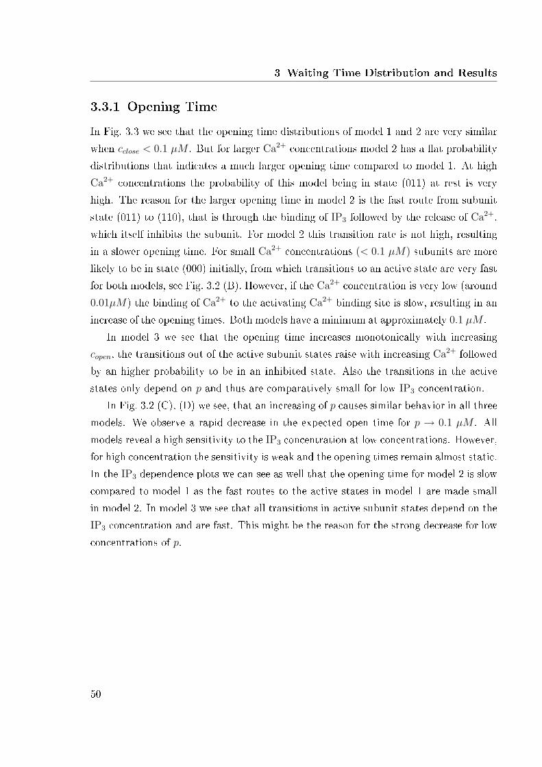
3 Waiting Time Distribution and Results

3.3.1 Opening TimeIn Fig. 3.3 we see that the opening time distributions of model 1 and 2 are very similarwhen cclose < 0.1 µM . But for larger Ca2+ concentrations model 2 has a �at probabilitydistributions that indicates a much larger opening time compared to model 1. At highCa2+ concentrations the probability of this model being in state (011) at rest is veryhigh. The reason for the larger opening time in model 2 is the fast route from subunitstate (011) to (110), that is through the binding of IP3 followed by the release of Ca2+,which itself inhibits the subunit. For model 2 this transition rate is not high, resultingin a slower opening time. For small Ca2+ concentrations (< 0.1 µM) subunits are morelikely to be in state (000) initially, from which transitions to an active state are very fastfor both models, see Fig. 3.2 (B). However, if the Ca2+ concentration is very low (around0.01µM) the binding of Ca2+ to the activating Ca2+ binding site is slow, resulting in anincrease of the opening times. Both models have a minimum at approximately 0.1 µM .

In model 3 we see that the opening time increases monotonically with increasingcopen, the transitions out of the active subunit states raise with increasing Ca2+ followedby an higher probability to be in an inhibited state. Also the transitions in the activestates only depend on p and thus are comparatively small for low IP3 concentration.

In Fig. 3.2 (C), (D) we see, that an increasing of p causes similar behavior in all threemodels. We observe a rapid decrease in the expected open time for p → 0.1 µM . Allmodels reveal a high sensitivity to the IP3 concentration at low concentrations. However,for high concentration the sensitivity is weak and the opening times remain almost static.In the IP3 dependence plots we can see as well that the opening time for model 2 is slowcompared to model 1 as the fast routes to the active states in model 1 are made smallin model 2. In model 3 we see that all transitions in active subunit states depend on theIP3 concentration and are fast. This might be the reason for the strong decrease for lowconcentrations of p.

50

3 Waiting Time Distribution and Results

0

0.5

1

1.5

2

2.5

0 1 2 3 4 5

Fop

en(A

,t) (

s-1)

Time (s)

Model 1

copen0.01 µM

0.1 µM10.0 µM

0

0.5

1

1.5

2

0 1 2 3 4 5

Fop

en(A

,t) (

s-1)

Time (s)

Model 2

copen0.01 µM

0.1 µM1.0 µM

0

0.5

1

1.5

2

2.5

3

0 1 2 3 4 5

Fop

en(A

,t) (

s-1)

Time (s)

Model 3

copen0.01 µM

0.1 µM1.0 µM

10.0 µM

0

5

10

15

20

0 0.2 0.4 0.6 0.8 1

Fop

en(A

,t) (

s-1)

Time (s)

Model 3

IP30.1 µM0.5 µM1.0 µM

0

1

2

3

4

5

0 1 2 3 4 5

Fop

en(A

,t) (

s-1)

Time (s)

Model 1

IP30.01 µM0.1 µM

10.0 µM

0

1

2

3

4

0 1 2 3 4 5

Fop

en(A

,t) (

s-1)

Time (s)

Model 2

IP30.01 µM0.05 µM10.0 µM

A

B

C

D

E

F

Figure 3.3: (A-C) Results of the opening time probability density distributionFopen(A, t) in dependence on the Ca2+ concentration for all three models. The Ca2+

concentration varies between 0.01− 10 µM . (D-F) Fopen(A, t) for all three models asfunction of the IP3 concentration, which is between 0.01− 10.0 µM .

51

3 Waiting Time Distribution and Results

0

0.2

0.4

0.6

0.8

1

1.2

1.4

40 80 120 160 200

Tcl

ose

(s)

cclose (µM)

Model 1

Model 2

Model 2 fast release

Model 3

0

0.2

0.4

0.6

0.8

1

0 2 4 6 8 10

Tcl

ose

(s)

p (µM)

Model 3Model 3

0

0.5

1

1.5

2

2.5

3

3.5

4

0 2 4 6 8 10

Tcl

ose

(s)

p (µM)

Model 1

Model 2

Model 1

Model 2

A

B C

Figure 3.4: Expected closing time Tclose, from both the analytic and simulation results.The continuous lines are the analytic results and the lines with symbols the simula-tions. (A) Expected closing time for model 1 (red), model 2 (blue), model 2 withfast IP3 release (turquoise) and model 3 (violet) as function of the Ca2+ concentra-tion. (B) Expected closing time for model 1 (blue) and 2 (red) in dependence on IP3

concentration and (C) results for model 3.

3.3.2 Closing TimeFig. 3.5 (A-C) show that changing the Ca2+ concentration has very little e�ect on theclosing time distribution of model 2 compared to model 1. This is because the Ca2+

dependent transition out of the active state is very slow in model 2 and thus the Ca2+

concentration has little e�ect on the closing time. In model 1, however, this transition isfast and causes a higher sensitivity to the Ca2+ concentration. In model 3 the transitionsinto inhibited states depend on the Ca2+ concentration, but they are slow and thefastest transition from O to S does not depend on any concentration resulting in a lowsensitivity.

52

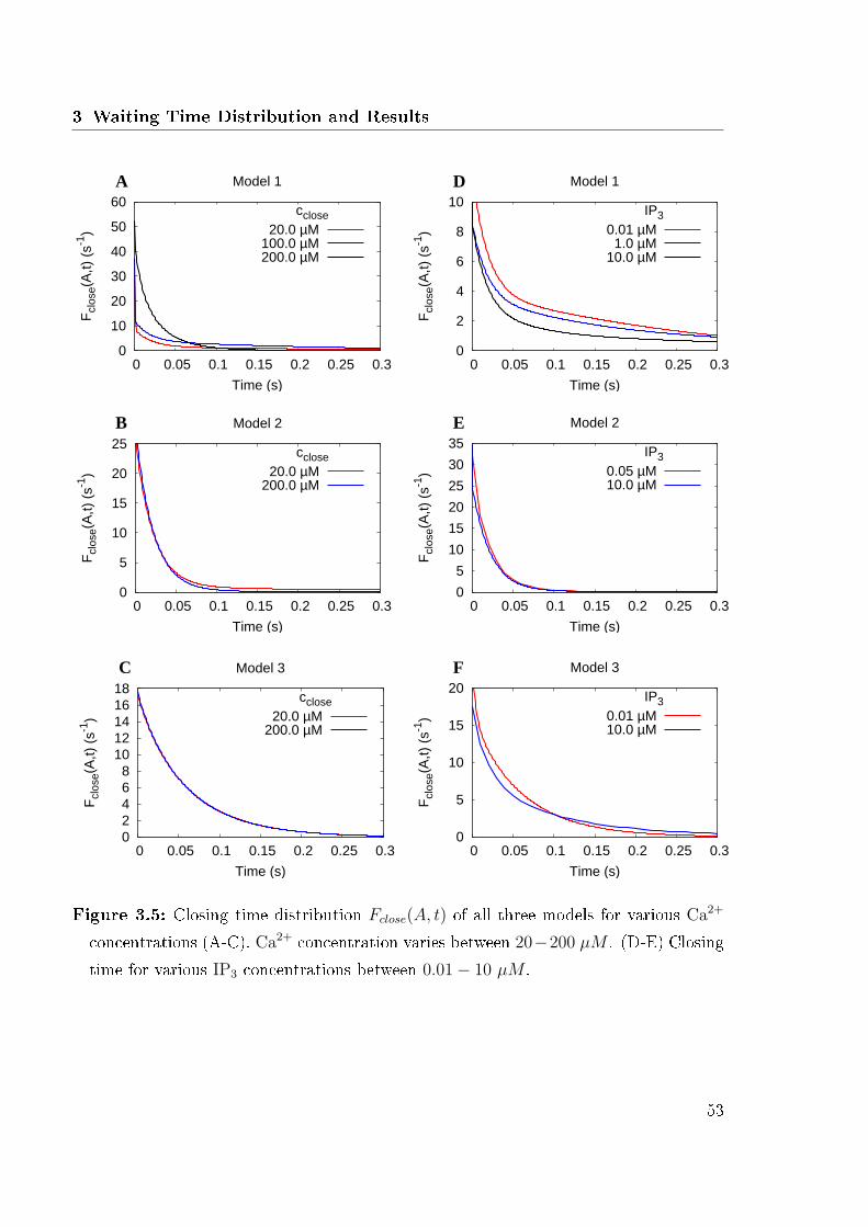
3 Waiting Time Distribution and Results

0

5

10

15

20

25

0 0.05 0.1 0.15 0.2 0.25 0.3

Fcl

ose(

A,t)

(s-1

)

Time (s)

Model 2

cclose20.0 µM

200.0 µM

0

2

4

6

8

10

0 0.05 0.1 0.15 0.2 0.25 0.3

Fcl

ose(

A,t)

(s-1

)

Time (s)

Model 1

IP30.01 µM1.0 µM

10.0 µM

0 2 4 6 8

10 12 14 16 18

0 0.05 0.1 0.15 0.2 0.25 0.3

Fcl

ose(

A,t)

(s-1

)

Time (s)

Model 3

cclose20.0 µM

200.0 µM

0

5

10

15

20

25

30

35

0 0.05 0.1 0.15 0.2 0.25 0.3

Fcl

ose(

A,t)

(s-1

)

Time (s)

Model 2

IP30.05 µM10.0 µM

0

5

10

15

20

0 0.05 0.1 0.15 0.2 0.25 0.3

Fcl

ose(

A,t)

(s-1

)

Time (s)

Model 3

IP30.01 µM10.0 µM

0

10

20

30

40

50

60

0 0.05 0.1 0.15 0.2 0.25 0.3

Fcl

ose(

A,t)

(s-1

)

Time (s)

Model 1

cclose20.0 µM

100.0 µM200.0 µM

A

B

C

D

E

F

Figure 3.5: Closing time distribution Fclose(A, t) of all three models for various Ca2+

concentrations (A-C). Ca2+ concentration varies between 20−200 µM . (D-E) Closingtime for various IP3 concentrations between 0.01− 10 µM .

53

3 Waiting Time Distribution and Results

Although all models show similar behavior at high Ca2+ concentrations model 1 closesquickly compared to model 2, due to the binding of inhibitory Ca2+. Model 1 showsthe strongest dependence on the Ca2+ concentration since the expected closing timedecreases rapidly with increasing Ca2+. Model 2 cannot bind inhibiting Ca2+ until IP3

has �rst been released, which results in slower closing times. To study this dependencemore precisely we increased the rate of IP3 release in model 2 by a factor of 10 (thatis K1 = 0.036 µM and K3 = 8.0 µM). We indicate this as model 2 fast release inFig. 3.4 (A). The change decreases the closing time signi�cantly. We also notice thatthe closing time for model 2 increases slightly with increasing Ca2+ concentration. Thise�ect disappears if we raise the IP3 release rate, consequently this transition might bethe reason for the rise. Logarithmic plots of opening and closing time distribution formodel 1 and 3, see Fig. 3.6, demonstrate di�erent time scales for opening and closingprocesses. We recognize clearly two di�erent time scales, which change at the thresholdc ∼ 0.1 µM . For Ca2+ concentrations > 0.1 µ the transition rate between states (110)and (100) dominates the opening time distribution for large Ca2+ concentrations. Inmodel 3 the dependencies are more complicated, nevertheless we notice similar behaviorwith two time scales. Model 1 has also two time scales dominating the closing process,whereas model 3 is governed by one transition from state O to S resulting in a clearexponential decrease.

Fig. 3.7 (A-C) shows that the number of inhibited channels increases for model1 with increasing Ca2+ concentration for Ca2+ > 50 µM. In model 2 instead, thenumber decreases with increasing Ca2+ and the limit is reached slower than in model1. In model 3 one cannot notice a di�erence for di�erent concentrations, whereas themaximum number of 5 is reached comparatively fast.

Fig. 3.4 (B),(C) show that in all three models the expected closing time increaseswith increasing IP3 concentration. Model 1 reveals the strongest dependence on the IP3

concentration. Model 2 is not sensitive, what is due to the slow IP3 dependent transitionrates again. Model 3 shows not a strong dependence on the IP3 concentration as well.Whereas we �nd a signi�cant di�erence between the analytic and simulation results forhigh values of IP3, see Fig. 3.4 (C).

To study the assumption of using �xed calcium concentration for all channels in thecluster during computing the closing time distribution we show in Fig. 3.7 (D-F) the

54

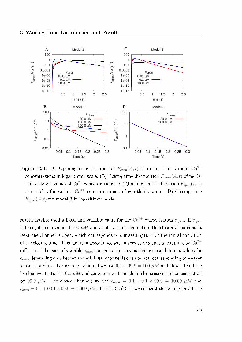
3 Waiting Time Distribution and Results

1e-12

1e-10

1e-08

1e-06

0.0001

0.01

1

100

0.5 1 1.5 2 2.5

Fop

en(A

,t) (

s-1)

Time (s)

Model 1

copen0.01 µM0.1 µM

10.0 µM

0.01

0.1

1

10

100

0.05 0.1 0.15 0.2 0.25 0.3

Fcl

ose(

A,t)

(s-1

)

Time (s)

Model 1

cclose20.0 µM

100.0 µM200.0 µM

1e-12

1e-10

1e-08

1e-06

0.0001

0.01

1

100

0.5 1 1.5 2 2.5

Fop

en(A

,t) (

s-1)

Time (s)

Model 3

copen0.01 µM0.1 µM

10.0 µM

0.1

1

10

100

0.05 0.1 0.15 0.2 0.25 0.3

Fcl

ose(

A,t)

(s-1

)

Time (s)

Model 3

cclose20.0 µM

200.0 µM

A

B

C

D

Figure 3.6: (A) Opening time distribution Fopen(A, t) of model 1 for various Ca2+

concentrations in logarithmic scale, (B) closing time distribution Fclose(A, t) of model1 for di�erent values of Ca2+ concentrations. (C) Opening time distribution Fopen(A, t)

of model 3 for various Ca2+ concentrations in logarithmic scale. (D) Closing timeFclose(A, t) for model 3 in logarithmic scale.

results having used a �xed and variable value for the Ca2+ concentration copen. If copen

is �xed, it has a value of 100 µM and applies to all channels in the cluster as soon as atleast one channel is open, which corresponds to our assumption for the initial conditionof the closing time. This fact is in accordance with a very strong spatial coupling by Ca2+

di�usion. The case of variable copen concentration means that we use di�erent values forcopen depending on whether an individual channel is open or not, corresponding to weakerspatial coupling. For an open channel we use 0.1 + 99.9 = 100 µM as before. The baselevel concentration is 0.1 µM and an opening of the channel increases the concentrationby 99.9 µM . For closed channels we use copen = 0.1 + 0.1 × 99.9 = 10.09 µM andcopen = 0.1+0.01× 99.9 = 1.099 µM . In Fig. 3.7(D-F) we see that this change has little

55

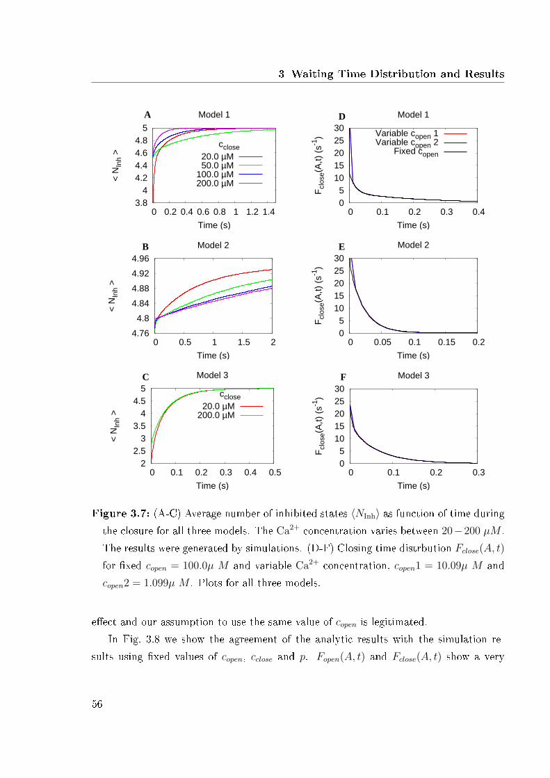
3 Waiting Time Distribution and Results

3.8 4

4.2 4.4 4.6 4.8

5

0 0.2 0.4 0.6 0.8 1 1.2 1.4

< N

Inh

>

Time (s)

Model 1

cclose20.0 µM50.0 µM

100.0 µM200.0 µM

4.76

4.8

4.84

4.88

4.92

4.96

0 0.5 1 1.5 2

< N

Inh

>

Time (s)

Model 2

2 2.5

3 3.5

4 4.5

5

0 0.1 0.2 0.3 0.4 0.5

< N

Inh

>

Time (s)

Model 3

cclose20.0 µM

200.0 µM

0 5

10 15 20 25 30

0 0.1 0.2 0.3 0.4

Fcl

ose(

A,t)

(s-1

)

Time (s)

Model 1

Variable copen 1Variable copen 2

Fixed copen

0 5

10 15 20 25 30

0 0.05 0.1 0.15 0.2

Fcl

ose(

A,t)

(s-1

)

Time (s)

Model 2

0 5

10 15 20 25 30

0 0.1 0.2 0.3

Fcl

ose(

A,t)

(s-1

)

Time (s)

Model 3

A

B

C

D

E

F

Figure 3.7: (A-C) Average number of inhibited states 〈NInh〉 as function of time duringthe closure for all three models. The Ca2+ concentration varies between 20−200 µM .The results were generated by simulations. (D-F) Closing time distrbution Fclose(A, t)

for �xed copen = 100.0µ M and variable Ca2+ concentration, copen1 = 10.09µ M andcopen2 = 1.099µ M . Plots for all three models.

e�ect and our assumption to use the same value of copen is legitimated.In Fig. 3.8 we show the agreement of the analytic results with the simulation re-

sults using �xed values of copen, cclose and p. Fopen(A, t) and Fclose(A, t) show a very

56

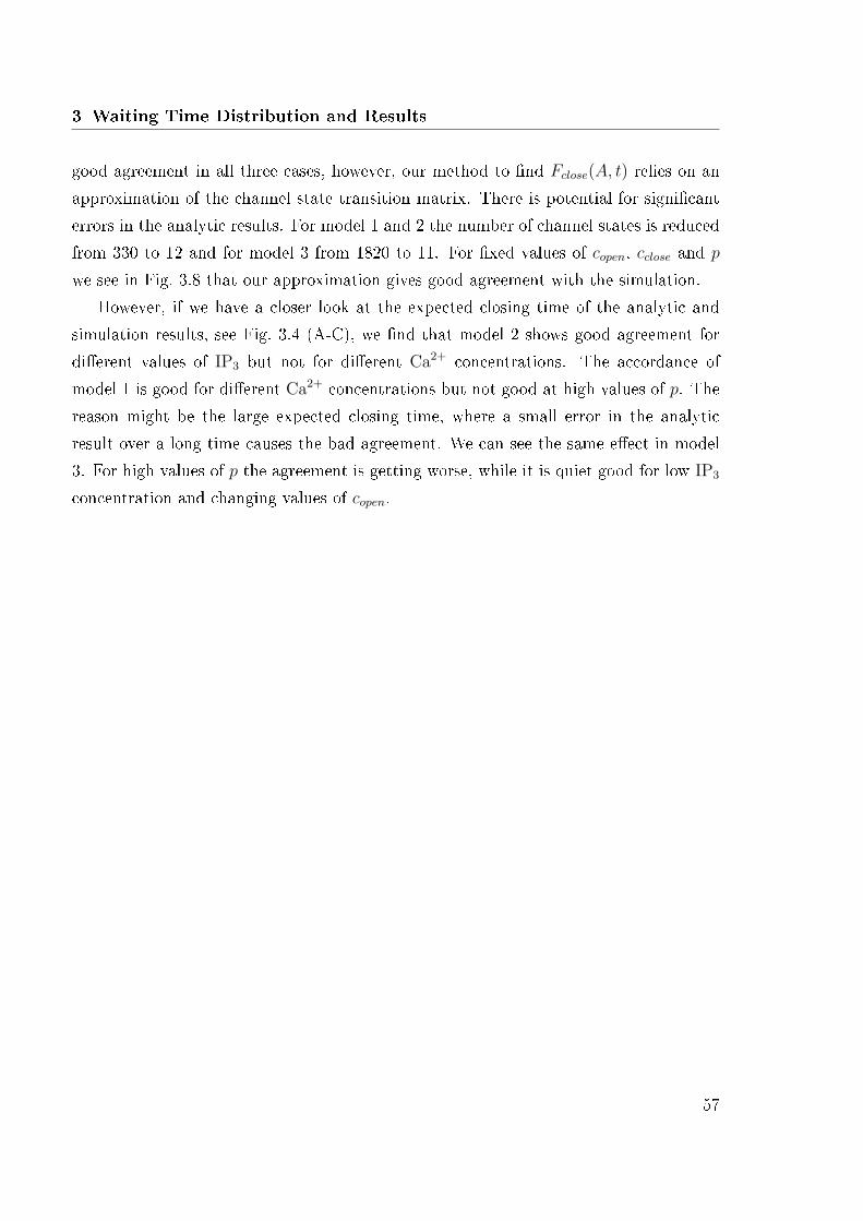
3 Waiting Time Distribution and Results

good agreement in all three cases, however, our method to �nd Fclose(A, t) relies on anapproximation of the channel state transition matrix. There is potential for signi�canterrors in the analytic results. For model 1 and 2 the number of channel states is reducedfrom 330 to 12 and for model 3 from 1820 to 11. For �xed values of copen, cclose and p

we see in Fig. 3.8 that our approximation gives good agreement with the simulation.However, if we have a closer look at the expected closing time of the analytic and

simulation results, see Fig. 3.4 (A-C), we �nd that model 2 shows good agreement fordi�erent values of IP3 but not for di�erent Ca2+ concentrations. The accordance ofmodel 1 is good for di�erent Ca2+ concentrations but not good at high values of p. Thereason might be the large expected closing time, where a small error in the analyticresult over a long time causes the bad agreement. We can see the same e�ect in model3. For high values of p the agreement is getting worse, while it is quiet good for low IP3

concentration and changing values of copen.

57

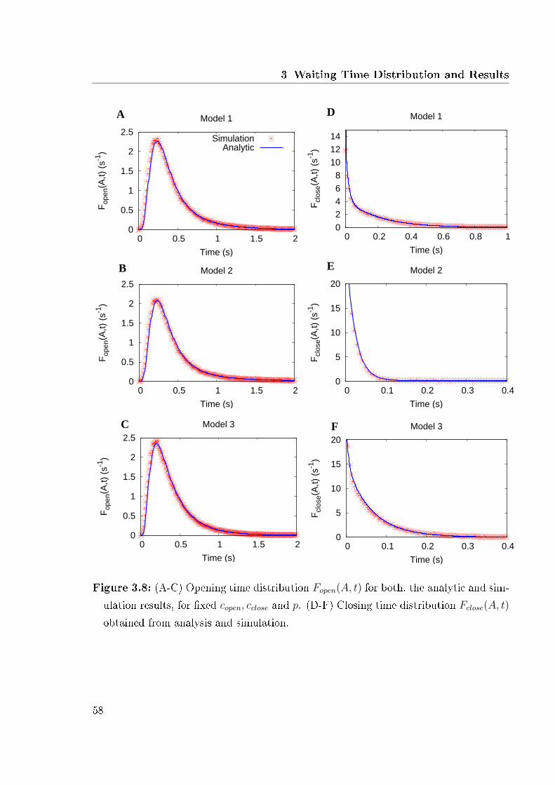
3 Waiting Time Distribution and Results

0

0.5

1

1.5

2

2.5

0 0.5 1 1.5 2

Fop

en(A

,t) (

s-1)

Time (s)

Model 1

SimulationAnalytic

0 2 4 6 8

10 12 14

0 0.2 0.4 0.6 0.8 1

Fcl

ose(

A,t)

(s-1

)

Time (s)

Model 1

0

5

10

15

20

0 0.1 0.2 0.3 0.4

Fcl

ose(

A,t)

(s-1

)

Time (s)

Model 2

0

5

10

15

20

0 0.1 0.2 0.3 0.4

Fcl

ose(

A,t)

(s-1

)

Time (s)

Model 3

0

0.5

1

1.5

2

2.5

0 0.5 1 1.5 2

Fop

en(A

,t) (

s-1)

Time (s)

Model 3

0

0.5

1

1.5

2

2.5

0 0.5 1 1.5 2

Fop

en(A

,t) (

s-1)

Time (s)

Model 2

A

B

C

D

E

F

Figure 3.8: (A-C) Opening time distribution Fopen(A, t) for both, the analytic and sim-ulation results, for �xed copen, cclose and p. (D-F) Closing time distribution Fclose(A, t)

obtained from analysis and simulation.

58

3 Waiting Time Distribution and Results

0.02

0.03

0.04

0.05

0.06

0.07

0.08

5 10 15 20 25 30

Tcl

ose

(s)

N

Model 1

1212

0 0.05

0.1 0.15

0.2 0.25

0.3 0.35

0.4

5 10 15 20 25 30

Tcl

ose

(s)

N

Model 2

1212

0

0.01

0.02

0.03

0.04

0.05

0.06

0.07

5 10 15 20 25 30

Tcl

ose

(s)

N

Model 3

11

1

2

3

4

5

6

7

8

50 100 150 200 250 300

Nop

en

N

Model 1

copen = 50.0 µMcopen = 100.0 µM

p = 10.0 µM

1

2

3

4

5

6

7

8

50 100 150 200 250 300

Nop

en

N

Model 2

0

10

20

30

40

50

60

70

0 400 800 1200 1600

Nop

en

N

Model 3

A

B

C

D

E

F

Figure 3.9: (A-C) Expected closing time Tclose as a function of the number of aggregatestates N . Results were produced with a single channel. The black vertical linesindicate the threshold of aggregate states in our calculations. The Ca2+ concentrationis 10 µM (black line), 50 µM (red line) and 100 µM (blue line). (D-F) Number ofopen aggregate states Nopen in dependence of the number of aggregate states N forthe same concentration values.

3.3.3 Criteria for ReductionFig. 3.9 shows how the expected closing time of a single channel behaves as the numberof aggregate states is reduced. We have used a single channel in these plots, as it is too

59

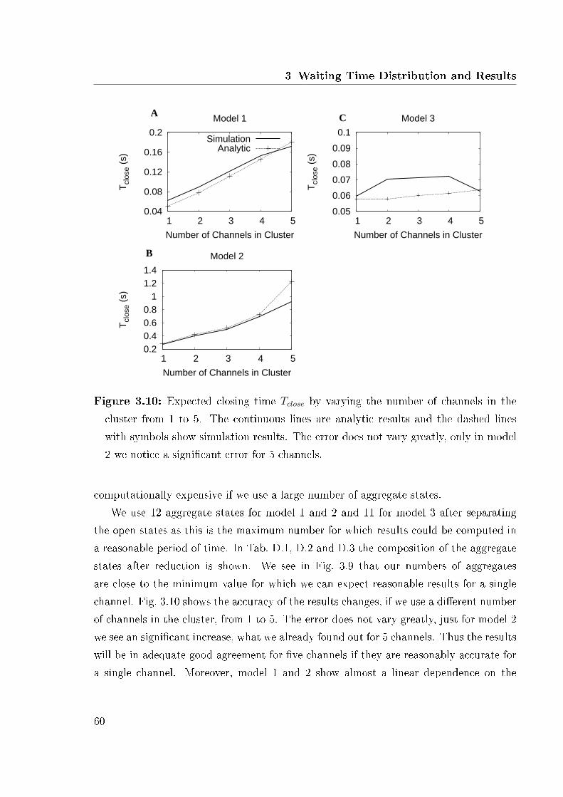
3 Waiting Time Distribution and Results

0.04

0.08

0.12

0.16

0.2

1 2 3 4 5

Tcl

ose

(s)

Number of Channels in Cluster

Model 1

SimulationAnalytic

0.2 0.4 0.6 0.8

1 1.2 1.4

1 2 3 4 5

Tcl

ose

(s)

Number of Channels in Cluster

Model 2

0.05

0.06

0.07

0.08

0.09

0.1

1 2 3 4 5

Tcl

ose

(s)

Number of Channels in Cluster

Model 3A

B

C

Figure 3.10: Expected closing time Tclose by varying the number of channels in thecluster from 1 to 5. The continuous lines are analytic results and the dashed lineswith symbols show simulation results. The error does not vary greatly, only in model2 we notice a signi�cant error for 5 channels.

computationally expensive if we use a large number of aggregate states.We use 12 aggregate states for model 1 and 2 and 11 for model 3 after separating

the open states as this is the maximum number for which results could be computed ina reasonable period of time. In Tab. D.1, D.2 and D.3 the composition of the aggregatestates after reduction is shown. We see in Fig. 3.9 that our numbers of aggregatesare close to the minimum value for which we can expect reasonable results for a singlechannel. Fig. 3.10 shows the accuracy of the results changes, if we use a di�erent numberof channels in the cluster, from 1 to 5. The error does not vary greatly, just for model 2we see an signi�cant increase, what we already found out for 5 channels. Thus the resultswill be in adequate good agreement for �ve channels if they are reasonably accurate fora single channel. Moreover, model 1 and 2 show almost a linear dependence on the

60

3 Waiting Time Distribution and Results

1

2

3

4

5 10 15 20 25

Nop

en

Number of Aggregates

Model 1

0.01

0.02

0.03

0.04

0.05

5 10 15 20 25

Tcl

ose

(s)

Number of Aggregates

Model 1BA

Figure 3.11: (A) Number of open aggregate states Nopen and (B) expected closing timeTclose for 2 channels in model 1 as function of the number of aggregate states.

number of channels in the cluster, whereas model 3 not.The method we suggest to be used is to compute the expected closing time for a

single channel using the full model and to compare this with the expected closing timecomputed after reducing the system. By plotting the expected closing time over thenumber of reduced states it is possible to �nd the minimum number for which reasonableresults can be expected. We can see that the expected closing time changes abruptlyif the number of aggregate states reaches a threshold. The plots in Fig. 3.9 (D-F)show how the number of open states changes with the number of aggregate states. Theabrupt change in the expected closing time corresponds to changes in the number of openaggregate states. The expected closing time is constant for a constant number of openstates, and always changes, although the changes are too subtle to be clear in the plots,when the number of open aggregate states changes. This could suggest that puttingtogether all open channels in one aggregate would improve the results. This is true for asingle channel, but not necessarily for multiple channels, since if we compute the closingtime distribution, all rows and columns in the cluster state matrix that correspond toclosed states were removed. For a single channel the cluster state transition matrixis the channel state transition matrix and closed cluster states are the same as closedchannel states. Hence, the number of closed aggregate states has no e�ect on the results,only the number of open aggregates. This explains why the expected open time changeswhen the number of open aggregate states changes. If there is more than one channel,changes in the expected opening time can occur while the number of open aggregate

61

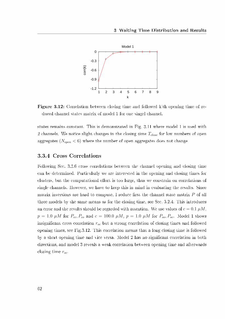
3 Waiting Time Distribution and Results

-1.2

-0.9

-0.6

-0.3

0

1 2 3 4 5 6 7 8 9

corr

(k)

k

Model 1

Figure 3.12: Correlation between closing time and followed k'th opening time of re-duced channel states matrix of model 1 for one singel channel.

states remains constant. This is demonstrated in Fig. 3.11 where model 1 is used with2 channels. We notice slight changes in the closing time Tclose for low numbers of openaggregates (Nopen < 6) where the number of open aggregates does not change

3.3.4 Cross CorrelationsFollowing Sec. 3.2.6 cross correlations between the channel opening and closing timecan be determined. Particularly we are interested in the opening and closing times forclusters, but the computational e�ort is too large, thus we constrain on correlations ofsingle channels. However, we have to keep this in mind in evaluating the results. Sincematrix inversions are hard to compute, I reduce �rst the channel state matrix P of allthree models by the same means as for the closing time, see Sec. 3.2.4. This introducesan error and the results should be regarded with attention. We use values of c = 0.1 µM ,p = 1.0 µM for Pcc, Pco and c = 100.0 µM , p = 1.0 µM for Poo, Poc. Model 1 showsinsigni�cant cross correlation roc but a strong correlation of closing times and followedopening times, see Fig.3.12. This correlation means that a long closing time is followedby a short opening time and vice versa. Model 2 has no signi�cant correlation in bothdirections, and model 3 reveals a weak correlation between opening time and afterwardsclosing time roc.

62

4 Discussion and Outlook

Many di�erent approaches to describe dynamics of IP3 gated Ca2+ channels have beenproposed [48, 35, 29, 19]. New experimental and theoretical �ndings reveal the stochasticcharacter of local and global Ca2+ release events. On this basis we have developed amethod to compute the opening and closing time probability distribution directly fromthe single channel subunit model using the Master Equation. We applied it to threedi�erent models. The �rst one is the one by Shuai et al. [38] and Rüdiger et al. [33] andis similar to the model of DeYoung and Keizer [50]. There are three binding sites, onefor IP3, one for activating Ca2+ and one for inhibitory Ca2+, resulting in a eight statesmodel. Shuai et al. and Rüdiger et al. extended the model with one 'Active' state, whichis only reachable from the state, where IP3 and activating Ca2+ is bound and inhibitoryCa2+ is not bound. We reduced these two states to one state by assuming the transitionsbetween them as fast. The second model is a modi�cation of the �rst one proposed byAdkins and Taylor [2]. They make the inhibitory Ca2+ binding rate small when IP3 isbound and also the activating Ca2+ rate when IP3 is not bound. The transition in theopposite direction are also made small to maintain detailed balance. The third modelis given by Sneyd and Dufour [41] and extended by Falcke [19] in order to overcome theproblem of Ca2+ conservation in the original model, what leads to thirteen states.

We used a cluster of 5 channels, because our method to calculate the cluster closingtime requires the number of channels in the cluster to be small (≤ 5) so that the numberof possible cluster states is not too large. In Fig. 4.1 we compare the computation timeof model 3. The opening time calculation shows no dependence, whereas the closingtime computation time increases extremely by using 6 channels. There have been manyestimates of the number of possible channels in a cluster. Some estimate the number tobe in the range of 20 - 30 [10, 15, 44], while Shuai et al. [37] estimate 40 - 70. However,Fraiman et al. [20] estimate 4 or 5, which agrees with the number estimated by Swillens

63

4 Discussion and Outlook

15

16

17

18

19

20

1 2 3 4 5 6

Tim

e (s

)

Number of Channels

Model 3

0

100

200

300

400

1 2 3 4 5 6

Tim

e (m

in)

Number of Channels

Model 3A B

Figure 4.1: (A) Computation time of opening time for various channels in cluster inmodel 3. (B) Computation time of closing time for model 3.

et al. [45]. New results [39] and Parker (not yet published) estimate the number to5-10 channels in a cluster. Our results con�rm these numbers, whereas the models showdi�erent dependencies on the number of channels in a cluster, see Fig. 3.10. Model 1and 2 depend almost linear on the number of channels, model 3 instead shows not thisbehavior.

It is important to remark that in all models transition rates depend on the Ca2+ andIP3 concentration. However, we neglect in�uences by di�erent temperatures. Experi-ments suggest, however, that Ca2+ dynamics depend on the temperature [34]. Biologicalsystem are far away from equilibrium, thus temperature �uctuations cannot be disre-garded in general. Nevertheless we don not take them into account because the detailsare not yet understood very well. The method I developed in the present diploma thesiscould be used to study temperature dependencies in detail.

The opening and closing time probability distributions resulting from all three modelsat various Ca2+ and IP3 concentrations gave signi�cantly di�erent results. Model 1 and2 have similar expected opening times at low Ca2+ concentration, both show a clearminimum at c ≈ 0.1 µM , but at larger concentrations model 2 has a much largerexpected opening time, see Fig. 3.2. This results from the activating and inhibitoryCa2+ binding site which are likely to be occupied for high Ca2+ concentrations. Hence,model 1 opens fast due to the binding of IP3, then it releases inhibitory Ca2+. In model2, however, this transition rates are very small resulting in a slower Ca2+ release.

64

4 Discussion and Outlook

The function of the expected opening time using model 1 and 2 is non monotonic.This is caused by the high probability to be in states, where Ca2+ and IP3 are notbound at the initial state and low Ca2+ concentrations. The transition from these statesto the active states is slow for low Ca2+ concentration and raises with increasing Ca2+

resulting in a minimum. Thus, for high Ca2+ concentration the subunits are likely tohave bound inhibitory Ca2+ at rest, what makes the transition the the active stateslower. Model 3 instead shows a weak linear behavior without a minimum, because thefew transitions from active to inhibited states depend on Ca2+, and thus increasing theCa2+ concentration leads to an slightly larger expected open time.

A very interesting point is that all three models have very similar behavior for variousIP3 concentrations, see Fig. 3.3 and Fig. 3.2. All of them have very high expected openingtimes for low IP3 concentrations. In model 3 the activation is weak at this concentrations,thus the expected open time is high. But an increase leads to a rapid reduce in theexpected opening time and for higher concentrations it stays almost constant. Model 1and 2 behave in an identical way, once again the opening time is larger for model 2.

The closing times reveal also signi�cantly di�erent behavior for all three models.Model 2, model 2 with fast IP3 release and model 3 do not depend strongly on the Ca2+

concentration, model 1 instead does. The reason is the Ca2+ dependent transitions intoinhibited states are high for model 1 and thus it is sensitive to the Ca2+ concentration.This transition is slow for model 2 and thus it is less sensitive. Increasing the rateat which IP3 is bound, decreased the expected closing time in model 2 but it was lesssensitive to Ca2+ concentration, too. Model 3 has low transition rates in inhibited states,which causes the low sensitivity. In all three models the expected closing time growswith increasing IP3 concentration, see Fig. 3.4, because the release of IP3 results ininactivation of subunits and thus in closure of channels. In model 1 and 2 the bindingof IP3 also reduces the a�nity of the inhibitory Ca2+ binding site, which causes thestronger dependence compared to model 3.

The di�erent behavior of the waiting time distributions of opening and closing time,see Fig. 3.3 and Fig. 3.5, is probably generated by the initial conditions. The openingtimes start at zero, have a clear maximum and show an exponential decrease, whereasthe closing times have a large contribution at t = 0 and decrease exponentially withoutmaximum. The reason for this fundamental di�erence in the characteristics is that the

65

4 Discussion and Outlook

initial state in the second case (closing time) is near the �nal state where all channels inthe cluster are closed states. That is, we assume the cluster state, with exactly one openchannel as initial state and the state with all channels closed as �nal state. Thus thedistance between both is just one channel changing state, what causes the contributionat t = 0. It is obvious that for the opening times the initial channel state has a larger'distance' to the �nal state, since we choose the distribution at rest. This multiplechannel changing state causes the behavior near t = 0 and the maximum. We obtain asimilar curve for the closing time with maximum if we choose e.g. 2 channels in a closedstate as the initial channel state.

Thul and Falcke [47] present a method for calculating opening time distributions forclusters of IP3 channels. Their method avoids the problem of computing eigenvaluesand eigenvectors of large matrices, but requires the roots of a polynomial of high orderto be found. The method of Thul and Falcke was not extended to cluster closing timedistributions. In this diploma thesis we were able to �nd the eigenvalues and eigenvectorsof the channel state transition matrices.

An important question is, if the assumption is correct, to use the same Ca2+ con-centration for all �ve channels, when we compute the cluster closing time. The initialcondition for the closing time is chosen by one channel in the cluster to be open, sincewe consider the cluster to be open when one channel in the cluster is open. We used a�xed and variable value for the Ca2+ concentration when the cluster is open. In Fig. 3.7(D-F) we see that using di�erent Ca2+ concentrations, wether the individual channel isopen or closed has very little impact on the result. Fraiman et al. [20] note that the timetaken for a single inactivated IP3 channel to become uninhibited is much smaller than atypical pu� duration. Our results support this statement. The Ca2+ concentration seenby closed channels has thus little e�ect, as all channels are likely to close before it hastime to reopen. This result implies that pu�s with these models are insensitive to spatialarrangement of individual channels within the cluster as long as the distance is not toolarge. We tested this statement by using two orders of magnitude (copen = 1.099 µM ,copen = 10.09 µM) corresponding to 4.6 di�usion lengths of free Ca2+ corresponding toa Ca2+ concentration of 100.0 µM .

In order to calculate the cluster closing time distribution, we reduced the channelstates transition matrix. We applied di�erent methods to reduce the system size of the

66

4 Discussion and Outlook

channel states transition matrix. Well known approaches in biochemistry are the QuasiSteady State Approximation and the Rapid Equilibrium Approximations [24, 36]. Forreasons of computation time the �rst reduction method is not practical. The secondmethod was not able to reduce the system size su�ciently. Thus we adapted the PerronCluster Analysis proposed by Deu�hard et al. [13] and achieved to develop a fast andstable reduction method to compute results in a reasonable time. We tested all methodson the 13 states subunit model proposed by Sneyd and Dufour [41] and Falcke [19].They successively reduced the dimension by combining two states that are connected bya large transition rate into one aggregate state. We compute transitions in and out ofthe new aggregate state. We found that the method combining the current information,by computing new transition rates in every reduction step, and the original informationby using the initial state distribution of the original channel state transition matrix,works best. We show in Appendix C that we �nd out nearly the same number ofclusters proposed by the Perron Cluster Analysis. Deu�hard et al. remark that exactdetermination of the number of clusters is very di�cult, but our approach leads to goodresults.

The state aggregation introduces, however, an error to the calculation, which is mostapparent in model 2, Fig. 3.4 (A), and for di�erent values of IP3 in model 1, see Fig. 3.4(B). In general the error becomes large for high values of the expected closing time ofall three models. Consequently, the error between the simulation and analytic resultsseems to be ampli�ed if it occurs over a long time range. Our criterion to stop combiningstates into aggregates if analytic results for a single channel get bad compared to singlechannel simulations was the most predictive and feasible criterium.

Comparison of our results to experimental �ndings [28, 30, 44] demonstrate thecapacity to reproduce cluster behavior. The stochastic character of Ca2+ release eventsis recently revealed [19, 40] and a�rmed by our results. We are able to reproducecorrect time scales of single opening events. Experimenters regulate the value of Ca2+

and IP3 concentration to 5 − 10 µM and 40 − 50 µM , respectively, by pretreatment.The agreement for high values of IP3 and Ca2+ are quiet good. Remark, that plots ofexperimental results show released Ca2+ but our plots show the probability distributionof a cluster opening or closing. Comparison of experimental data and our theoreticalresults should be made by keeping this in mind. The expected opening and closing time

67

4 Discussion and Outlook

can not predicate the amount of released Ca2+.However, we remark that the opening time depends strongly on the base level Ca2+

concentration, and thus to evaluate our results in more detail more advanced experi-ments are required. For example measurements of release events as function of the Ca2+

concentration would be very helpful. Fraiman et al. [20] revealed correlations of pu�amplitude and interpu� interval. Our results reveal almost no correlation between open-ing and closing times, just model 1 shows a signi�cant correlation. Since we simplify thesystem enormous one should handle this result with care.

To summarize the results, it is important to notice that our analytic method revealedclearly di�erent behavior of all three models. These di�erent characteristics could beused by experimenters to gain deeper knowledge about the structure of Ca2+ channels.

Further steps could be to determine the opening duration time and by this meansto estimate the amount of released Ca2+. This can be used to compare analytic resultsdirectly with experimental data. Also interpu� time or the second opening time ofclusters are interesting points, which can be derived from the basis in this diplomathesis. The reduction method we developed could be improved and studied in moredetail in order to reveal the reason of its accuracy. Furthermore, the method of crosscorrelation could be meliorated to apply it to larger systems without simpli�cations.Stochastic cell models based on the method I developed in the present diploma thesisare very important. Computation of waiting time distributions of opening and closingtime for several clusters in a cell could provide new insights in cell mechanisms.

68

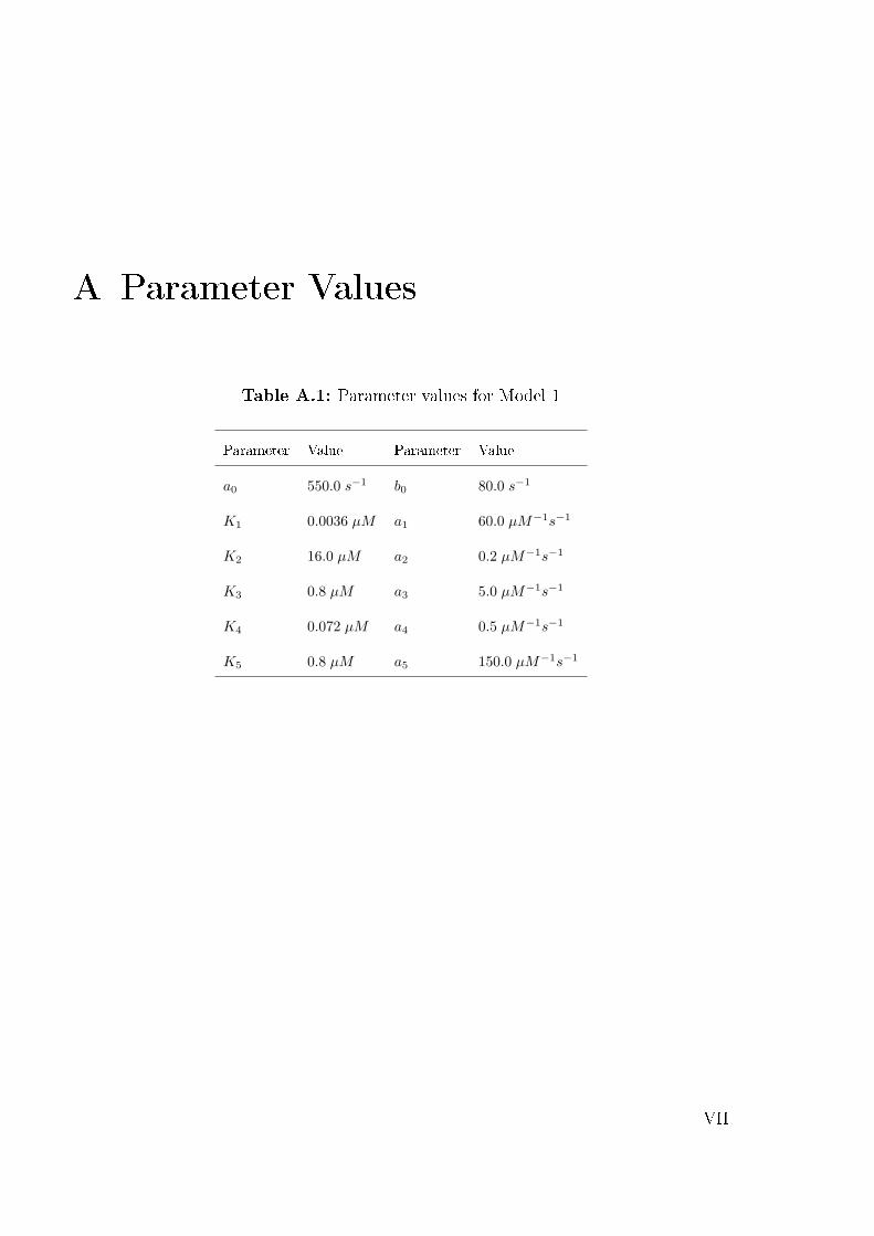
A Parameter Values

Table A.1: Parameter values for Model 1

Parameter Value Parameter Value

a0 550.0 s−1 b0 80.0 s−1

K1 0.0036 µM a1 60.0 µM−1s−1

K2 16.0 µM a2 0.2 µM−1s−1

K3 0.8 µM a3 5.0 µM−1s−1

K4 0.072 µM a4 0.5 µM−1s−1

K5 0.8 µM a5 150.0 µM−1s−1

VII

A Parameter Values

Table A.2: Parameter values for Model 3

Parameter Value Parameter Value

k1 2.0 µM−1s−1 k−1 0.04 s−1

k2 37.4 µM−1s−1 k−2 1.4 s−1

k3 0.11 s−1 k−3 29.8 s−1

k4 4.0 µM−1s−1 k−4 0.37 s−1

k5 2.0 µM−1s−1 l1 10.0 µM−1s−1

l3 100.0 µM−1s−1 l5 0.1 µM−1s−1

L1 0.12 µM L3 0.025 µM

L5 38.2 µM l2 1.7 s−1

l−2 0.8s−1 l4 37.4 µM−1s−1

l−4 2.5 s−1 l6 4707.0 s−1

l−6 11.4 s−1

VIII

B Proofs

B.1 Proof of Existence of Long Time LimitThe proof of Long Time Limit can be found in van Kampen [27].

We want to prove that all solutions tend to the stationary solution as t → ∞. LetΦ(t) be any solution of the Master Equation. At a positive time t the positive, negativeand zero components are distinguished

Φu(t) > 0, Φv(t) < 0, Φw = 0. (B.1)

withU(t) =

∑u

Φu(t), (B.2)

obviously U(t) is positive.

Lemma B.1.1 U(t) is a monotonic non increasing function of t.

With (2.21) we get

U(t) =∑

u

Φu =∑

u

(∑

u′Wuu′Φu′ +

∑

v′Wuv′Φv′

)

=∑

u′

(−

∑v

Wvu′ −∑

w

Wwu′

)Φu′ +

∑

v′

(∑u

Wuv′

)Φv′ .

(B.3)

Each term is non positive and soU(t) ≤ 0. (B.4)

If a term enters or leave the sum of U(t) at an instant, the term is zero at this instantand thus U(t) is continuous everywhere but not di�erentiable at a discrete set of points.Thus it cannot increase, what proves the lemma.

IX

B Proofs

We de�neV (t) =

∑v

Φv(t). (B.5)

V (t) is non decreasing since V + U = const, since V + U is the solution of the MasterEquation. Hence, if initially Φn(0) ≥ 0 for all n, then Φn(t) ≥ 0 for all t > 0. Ifthis would not be ful�lled, the Master Equation would not describe the evolution of aprobability distribution.

From (B.4) we see that U(t) tends to a limit and thus also V (t).

Lemma B.1.2 Unless W is decomposable or of splitting type at least one of these lim-iting values must vanish, so that ultimately all Φn(t) have the same sign or are zero,which is determined by the initial value Φn(t) = const = C.

We suppose that C ≥ 0 and prove V (∞) = 0. We note that U(∞) = 0, which canhappen if each of the terms in (B.3) vanish. We di�er several cases.

i. The set of components u is empty, i.e. Φu(∞) ≤ 0 for all u. As we choose C ≥ 0

this implies Φn(∞) = 0 and U(∞) = V (∞) = 0.

ii. The set of componontes u is not empty, but both set of components v and w are,then V (∞) = 0.

iii. Neither the set of components u and v are empty, but the set of components w is.Then one must have Wvu′ = Wuv′ = 0, so that W has the form

(Wuu′ 0

0 Wvv′

)(B.6)

so W is decomposable and is excluded from the lemma.

iv. None of the sets u, v, w is empty. Then one must have Wvu′ = Wwu′ = Wuv′ = 0,so that W has the form

Wuu′ 0 Wuw′

0 Wvv′ Wvw′

0 Wwu′ Www′

. (B.7)

X

B Proofs

Thus W is reducible. If we write down the analog of (B.3) for V (t) we can �nd thatWwv′ = 0, so that W is of splitting type and excluded from the lemma. This proves thesecond lemma.

For a time independent solution either all components are non negative, or all nonpositive. For a stationary probability solution one has ps

n ≥ 0 because C = 1.If p

(1)n (t) and p

(2)n (t) are two probability distributions satisfying the Master Equation

that is neither decomposable nor splitting. Thus Φn(t) = p(1)n (t) − p

(2)n (t) is a solution

for which C = 0 and soΦn(t) = p(1)

n (t)− p(2)n (t)→ 0. (B.8)

We see there can be not more than one stationary distribution, what completes theproof.

B.2 Proof of Detailed BalanceWe regard closed, isolated, physical systems, i.e. no exchange of matter with the externalworld takes place, and no external time dependent force acts on the system so that theenergy is a constant of motion. We want to prove Detailed Balance following van Kampen[27].

W (y|y′)P e(y′) = W (y′|y)P e(y) (B.9)

with W the transition matrix and P e the equilibrium distribution. We start the proofby abbreviate the notation. Let the point (q, p) in the phase space Γ be denoted by xand let xτ = (q′, p′) be the point into which the system is transported in the time τ andx = (q,−p) so that ¯x = x. Time reversal invariance is then expressed by

(xτ )τ = x xτ = (x)−τ . (B.10)

The bar operator also conserves the volume in Γ dx = dx. As a consequence we haveYx(0) = Yx(0) from which follows

Yx(t) = Yxt(0) = Y ¯x−t(0) = Yx(−t). (B.11)

The equilibrium distribution is a function of the constants of the motion, so we have

P e(x) = P e(x). (B.12)

XI

B Proofs

We can write the probability to be in state y2 at time τ if the system was in state y1 att = 0

P2(y1, 0; y2, τ) =

∫δ[y1 − Yx(0)]δ[y2 − Yx(τ)]P e(x)dx (B.13)

change the integration variable from x to x and use the previous conditions (B.11),(B.12), so we obtain

P2(y1, 0; y2, τ) =

∫δ[y1 − Yx(0)]δ[y2 − Yx(−τ)]P e(x)dx

= P2(y1, 0; y2,−τ) = P2(y2, 0; y1, τ).

(B.14)

This we can translate into an equation for P1,1

P1,1(y2, τ |y1, 0)P e(y1) = P1,1(y1, τ |y2, 0)P e(y2) (B.15)

and with the variable Y are such that Y (t) is a Markov Process, this relation may bewritten

Tτ (y2|y1)Pe(y1) = Tτ (y1|y2)P

e(y2). (B.16)

This is the result and we have proved (2.28).If the Hamiltonian of the system is not a even function, for example if there is

an external magnetic �eld B with vector potential A, then the Hamiltonian contains(p − eA)2 instead of p and does not remain the same on replacing p by −p. However,this can be remedied by simultaneous changing the sign of the �eld, so we get

W (y|y′; B)P e(y′) = W (y′|y;−B)P e(y). (B.17)

XII

C Perron Cluster

0.75

0.8

0.85

0.9

0.95

1

310 315 320 325 330

λ

Number of Eigenvalue

Model 1

0.65

0.7

0.75

0.8

0.85

0.9

0.95

1

310 315 320 325 330

λ

Number of Eigenvalue

Model 2

0.95

0.96

0.97

0.98

0.99

1

1808 1812 1816 1820

λNumber of Eigenvalue

Model 3

Figure C.1: Perron Cluster Analysis for all three models. We notice a gap after 5 and13 eigenvalues (A) for model 1 after 9 and 12 values for model 2 (B) and after 10 and13 for model 3 (C).

We show the results of Perron Cluster Analysis applied to the channel states transi-tion matrices obtained by all three models. That is, we plot in Fig. C.1 sorted eigenvaluesnear the maximum of 1. As mentioned above, see Sec. 2.2.4, the eigenvalues of nearlyuncoupled markov processes are grouped in a cluster near the Perron Root λ = 1.According to [13, 14] it is, however, di�cult to identify the clusters.

We remark that with our reduction method we are able to �nd out approximatelythe right number of clusters. Fig. C.1 Model 1 supposes that the channel states consistof maybe 5 or 13 clusters, since we remark a clear gap. Our method broke down afterwe reduced the system to 12 aggregate states. For di�erent concentrations of Ca2+ andIP3 the minimal number of aggregate states changed from 10 to 13. This fact shows thesensibility of the reduction process and that the identi�cation of the minimal number ofsubsystems is very di�cult. The same e�ect can be seen in Fig. C.1 model 2 and model3. For model 2 we identify 9 or 12 clusters, what corresponds very good with our resultsand for model 3 we identify 10 or 13 clusters, whereas our method reduced the systemto a minimal number of 11.

XIII

C Perron Cluster

XIV

D Aggregate States Composition

After reducing the channel states transition matrix for all three models, we get ancomposition of aggregate states. I show the results of the composition, i.e. the numberof inhibited, uninhibited and active states in aggregate states.

Table D.1: Model 1 Aggregate State Compositions

Aggregate No. No. Inhibited States No. Uninhibited Closed States No. Open States

1 83 8 0

2 60 12 0

3 21 12 0

4 0 6 0

5 0 3 0

6 0 12 0

7 9 21 0

8 20 20 0

9 22 13 0

10 0 0 2

11 0 0 2

12 0 0 4

XV

D Aggregate States Composition

Table D.2: Model 2 Aggregate State Compositions

Aggregate No. No. Inhibited States No. Uninhibited Closed States No. Open States

1 31 4 0

2 32 8 0

3 18 12 0

4 0 12 0

5 0 3 0

6 74 17 0

7 48 24 0

8 12 21 0

9 0 6 0

10 0 0 4

11 0 0 2

12 0 0 2

XVI

D Aggregate States Composition

Table D.3: Model 3 Aggregate State Compositions

Aggregate No. No. Inhibited States No. Uninhibited Closed States No. Open States

1 14 1 0

2 190 120 0

3 432 156 0

4 414 108 0

5 220 40 0

6 55 0 0

7 4 0 5

8 0 0 12

9 0 0 18

10 0 0 20

11 0 0 15

XVII

D Aggregate States Composition

XVIII

Bibliography

[1] http://�g.cox.miami.edu/ cmally/150/membs/cellcomm.htm.

[2] C. Adkins and C. Taylor. Lateral inhibition of inositol 1,4,5-trisphosphate receptorsby cytosolic Ca2+. Curr. Biol., 9(19):1115�8, 1999.

[3] B. Alberts, D. Bray, J. Lewis, M. Ra�, K. Roberts, and J. Watson. MolecularBiology of the Cell. Garland Publishing Inc., 1994.

[4] E. Anderson, Z. Bai, C. Bischof, S. Blackford, J. Demmel, J. Dongarra, J. Du Croz,A. Greenbaum, S. Hammarling, A. McKenney, and D. Sorensen. LAPACK Users'Guide. Society for Industrial and Applied Mathematics, 1999.

[5] F. Ball, C. Kerry, R. Ramsey, M. Sansom, and P. Usherwood. The use of dwelltime cross-correlation functions to study single.ion channel gating kinetics. Biophy.J., 54:309�320, 1988.

[6] F. Ball, R. Milne, and G. Yeo. Stochastic models for systems of interacting ionchannels. IMA Journal of Medicine and Biology, 17:263�293, 2000.

[7] F. Ball, G. Yeo, R. Milne, R. Edeson, and B. Madsen. Single ion channel modelsincorporating aggregation and time interval omission. Biophy. J, 64:357�374, 1993.

[8] M. Berridge, M. Bootman, and P. Lipp. Calcium-a life and death signal. Nature,395(6703):645�8, 1998.

[9] M. Berridge, M. Bootman, and P. Lipp. The versatility and universality of calciumsignaling. Nature Reviews, 1(1):11�21, 2000.

XIX

Bibliography

[10] N. Callamaras, J. Marchant, X-P. Sun, and I. Parker. Activation and coordinationof InsP3 mediated elementary Ca2+ release events during global Ca2+ signals inxenopus oocytes. J. Physiol., 509:81�91, 1998.

[11] D. Colquhoun and A. Hawkes. On the stochastic properties of burst of single ionchannel openings and of clusters of burst. Phil. Trans. R. Soc. Lond., 300:1�59,1982.

[12] C.W.Gardiner. Handbook of Stochastic Methods. Springer, 1985.

[13] P. Deu�hard, W. Huisinga, A. Fischer, and Ch. Schütte. Identi�cation of almostinvariant aggregates in reversible nearly uncoupled markov chains. Revised ZIBpreprint SC-98-03, 1998.

[14] P. Deu�hard and M. Weber. Robust perron cluster analysis in conformation dy-namics. ZIB-Report 03-19, 2003.

[15] G. Dupont and S. Swillens. Quantal release, incremental detection and long pe-riod Ca2+ oscillations in a model based on regulatory Ca2+-binding sites along thepermeation pathway. Biophys. J., 71(4):1714�1722, 1995.

[16] Lodish et al. Molecular Cell Biology. W.H. Freeman and Company, 2004.

[17] M. Falcke. Deterministic and stochastic models of intracellular Ca2+ waves. NewJournal of Physics, 5:96.1�96.28, 2003.

[18] M. Falcke. On the role of stochastic channel behaviour in intracellular Ca2+ dy-namics. Biophys. J., 84:42�56, 2003.

[19] M. Falcke. Reading the patterns in living cells - the physics of Ca2+ signaling. Adv.Phys., 53:255�440, 2004.

[20] D. Fraiman, B. Pando, S. Dargan, I. Parker, and S. Dawson. Analysis of pu�dynamics in oocytes: Interdependence of pu� amplitude and interpu� interval.Biophys. J., 90:3897�3907, 2006.

[21] D. Gillespie. Exact stochastic simulation of coupled chemical reactions. The Journalof Physical Chemistry, 81:2340�2361, 1977.

XX

Bibliography

[22] D. Gillespie. Markov Processes. Academic Press Inc., 1992.

[23] G. Golub and C. Loan. Matrix Computations. Johns Hopkins Studies in the Math-ematical Sciences, 1996.

[24] R. Heinrich and S. Schuster. The Regultation of Cellular Systems. Chapman andHall, 1996.

[25] J.Honerkamp. Stochastische Dynamische Systeme. VCH, 1990.

[26] Q. Jian, E. Thrower, D. Chester, B. Ehrlich, and F. Siegworth. Three dimensionalstructure of type 1 inositol 1,4,5-trisphosphate receptor at 24 angstrom resolution.EMBO J., 21(14):3575�3581, 2002.

[27] N.G.van Kampen. Stochstic Processes in Physics and Chemistry. North-Holland,1992.

[28] K. Machaca. Increased sensitivity and clustering of elementary Ca2+ release eventsduring oocyte maturation. Developmental Biology, 275:170�182, 2004.

[29] T. Meyer and L. Stryer. Calcium spiking. Annu. Rev. Biophys, 20:153�174, 1991.

[30] I. Parker and Y. Yao. Ca2+ transients associated with opening of inositol trisphos-phate gated channels in xenopus oocytes. J. Physiol., 491:663�668, 1996.

[31] W. Press, S. Teukolsky, W. Vetterling, and B. Flannery. Numerical Recipes in C++.Cambridge University Press, 2002.

[32] A. Quarteroni, R. Sacco, and F. Saleri. Numerische Mathematik I. Springer-VerlagBerlin Heidelberg New York, 2000.

[33] S. Rüdiger, J. Shuai, W Huisinga, C. Nagaiah, G. Warnecke, I. Parker, and M. Fal-cke. Hybrid stochastic and deterministic simulations of calcium blips. Biophysic.Journal, 93:1847�1857, 2007.

[34] C. Schipke, A. Heidemann, A. Skupin, O. Peters, M. Falcke, and H. Kettenmann.Temperature and nitric oxide control spontaneous calcium transients in astrocytes.Cell Calcium, pages 285�295, 2008.

XXI

Bibliography

[35] S. Schuster, M. Marhl, and T. Höfer. Modelling of simple and complex calciumoscillations. Eur. J. Biochem., 269:1333�1355, 2002.

[36] L. Segel and M. Slemrod. The quasi-steady-state assumption: A case study inperturbation. Society For Industrial and Applied Mathematics, 31:446�477, 1989.

[37] J. Shuai, J. Pearson, J. Foskett, D. Mak, and I. Parker. A kinetic model of sin-gle clustered IP3 receptors in the absence of Ca2+ feedback. Biophysic. Journal,93:1151�1162, 2007.

[38] W. Shuai and P. Jung. Stochastic properties of Ca2+ release of inositol 1,4,5-trisphosphate receptor clusters. Biophys. J., 83:87�97, 2002.

[39] A. Skupin and M. Falcke. The role of IP3r clustering in Ca2+ signaling. GenomeInformatics (accepted), 2008.

[40] A. Skupin, H. Kettemann, U. Winkler, M. Wartenebrg, H. Sauer, S. Tovey, C. Tay-lor, and M. Falcke. How does intracellular Ca2+ oscillate: By chance or by clock?Biophys. J., 94:2404�2411, 2008.

[41] J. Sneyd and J. Dufour. A dynamic model of the type-2 inositol trisphosphatereceptor. Proc. Natl. Acad. Sci, 99:2398�2403, 2002.

[42] J. Sneyd and M. Falcke. Models of the inositol trisphosphate receptor. Prog.Biophys. Mol. Bio., 89(3):207�45, 2005.

[43] M. Stern, G. Pizarro, and E. Rios. Local control model of excitation-concentrationcoupling in skeletal muscle. J. Gen. Physiol., 10:415�440, 1997.

[44] X-P. Sun, N. Callamaras, and I. Parker J. Marchan and. A continuum of InsP3 medi-ated elementary Ca2+ signalling events in xenopus oocytes. J. Physiol., 509.1:67�80,1998.

[45] S. Swillens, G. Dupont, L. Conbettes, and P. Champell. From calcium blips to cal-cium pu�s: theoretical analysis of the requirements for interchannel communication.Proc. Natl. Sci., 96:13750�13755, 1999.

XXII

Bibliography

[46] R. Thul and M. Falcke. Stability of membrane bound reactions. Phys. Rev. Lett.,29:93(18), 2004.

[47] R. Thul and M. Falcke. Waiting time distributions for clusters of complex molecules.Europhysics Letters, 79:38003, 2007.

[48] Y. Tuang, J. Stephenson, and H. Othmer. Simpli�cation and analysis of models ofcalcium dynamics based on InsP3-sensitive calcium channel kinetics. Biophys. J.,70:246�263, 1996.

[49] G. Ullah and P. Jung. Modeling the statistics of elementary calcium release events.Biophys. J., 90:3485�3495, 2006.

[50] G. De Young and J. Keizer. A single-pool inositol 1,4,5-trisphosphate-receptor basedmodel for agonist-stimulated oscillations in Ca2+ concentration. Proc. Natl. Acad.Sci, 89(20):9895�9899, 1992.

XXIII

Bibliography

XXIV

Acknowledgments

My special thanks go to my supervisor PD Dr. Martin Falcke who inroduced me into thefascinating �eld of Biophysics and Cell Dynamics and enabled me to write this diplomathesis and also to Prof. Dr. Jürgern Bosse who agreed on supervising my Diploma thesisas an external examiner.

I would like to thank Alexander Skupin who gave me many helpful advises in the �eldof Calcium Signaling and programming in C++. Special thanks go to Kevin Thurleywhose help and suggestions improved this diploma thesis enormously.

I am indebted to my student fellows Markus Düttmann and Christian Graf, whocorrected my work with patience.

Moreover I want to thank all members of the group who helped me with inspiringand enriching discussions.

Bibliography

XXVI

Erklärung der Urheberschaft

Ich erkläre hiermit an Eides statt, dass ich die vorliegende Arbeit ohne Hilfe Dritterund ohne Benutzung anderer als der angegebenen Hilfsmittel angefertigt habe; die ausfremden Quellen direkt oder indirekt übernommenen Gedanken sind als solche kenntlichgemacht. Die Arbeit wurde bisher in gleicher oder ähnlicher Form in keiner anderenPrüfungsbehörde vorgelegt.

Ort, Datum Unterschrift