Wages, Employment and Economic Shocks: Evidence from Indonesia

James P. Smith, Duncan Thomas, Elizabeth Frankenberg, Kathleen Beegle, Graciela Teruel

June 2000

This draft paper is intended to transmit preliminary results of IFLS research. It has not been formally reviewed or edited. The views and conclusions expressed are tentative. This draft should not be cited or quoted without permission of the author, unless the preface grants such permission.

Wages, employment and economic shocks:Evidence from Indonesia

James P. SmithRAND

Duncan ThomasRAND and UCLA

Elizabeth FrankenbergRAND

Kathleen BeegleRAND

Graciela TeruelUIA

First version: October, 1999This version: June, 2000

We have benefited from the comments of two referees, Thomas Bauer, Kai Kaiser and Jack Molyneaux. Wethank the Badan Pusat Statistik, Indonesia, for permission to use their annual labor force surveys. We also thankour colleagues at RAND, Lembaga Demografi, UCLA and the Population Study Centers in Indonesia whoworked with us in the collection of the Indonesia Family Life Survey; we are especially grateful to BondanSikoki, Wayan Suriastini, Muda Saputra and Cecep Sumantri. Financial support from the National Institutes ofAging (NIA P01AG08291) and the National Institute of Child Health and Human Development (NICHD1R01HD33778, 5P50HD12639 and 5P01HD28372) as well as the POLICY Project, World Bank and WorldHealth Organization are gratefully acknowledged.

Abstract

After over a quarter century of sustained economic growth, Indonesia was struck by a largeand unanticipated crisis at the end of the 20th Century. Real GDP declined by about 12%in 1998. Using 13 years of annual labor force data in conjunction with two waves of ahousehold panel, the Indonesia Family Life Survey (IFLS), this paper examines the impactof the crisis on labor market outcomes. Aggregate employment has remained remarkablyrobust through the crisis although there has been significant switching within sectors. Thedrama of the crisis lies not in aggregate employment but in real hourly earnings which, inone year, collapsed by around 40% for urban workers -- be they males or females, in themarket sector or self-employed. Declines of the same magnitude are recorded for femalesin the rural sector and rural males working for a wage. In stark contrast, real hourlyearnings of self-employed males in rural areas have remained essentially stable. Given theseworkers account for about one quarter of the male work force in Indonesia, conclusionsabout the effects of the crisis that focus only on the market wage sector substantially over-state the magnitude of the crisis. Indonesian families have displayed a remarkable capacityfor resilience in the face of the crisis. We estimate that declines in real family incomes areabout half the magnitude of the declines in individual hourly earnings indicating thathouseholds have adopted strategies to mitigate the effects of the crisis. Those strategiesappear to have been most successful for those at the top of the income distribution. At thebottom of the income distribution, the crisis has had a devastating impact on real incomessuggesting that it is the poorest who will likely bear the brunt of any deleterious mediumand longer-term effects of the crisis.

Introduction

After over a quarter century of sustained economic growth, Indonesia was struck by a major

economic crisis at the end of the 20th Century. The crisis, which worked its way through many of the

South East Asian "tigers" was presaged by the collapse of the Thai baht in the middle of 1997. During the

second half of the year, the Indonesian central bank attempted to stave off pressure on its currency, the

rupiah. Interest rates quadrupled and the rupiah depreciated by about 60%. In January 1998, the rupiah

collapsed. It lost about 75% of its value in a matter of a few days. The collapse of the rupiah was

followed by spiralling prices; annual inflation is estimated to be about 80% for 1998.

The impact of the crisis in Indonesia was not confined to the financial sector. The economy went

into a tailspin. Real output in 1998 was estimated to have been about 12% below its 1997 level (a bad

year for some because of the drought due to El Nino) and economic growth turned positive only in 2000.

The crisis was accompanied by dramatic and far-reaching political change.

By any metric, the crisis in Indonesia has been extremely severe -- far more severe than in any of

its South East Asian neighbors. For example, a year after the crisis began, the Thai baht and Philippine

peso stood at about half their pre-crisis values; the Indonesian rupiah had fallen to about one-quarter its

1997 value. A collapse of this magnitude is not unique: the Russian rouble and Ecuadoran sucre were both

reduced to one-quarter of their value over twelve months in 1998/1999. Relative to the Russian and

Ecuadoran crises, the crisis in Indonesia was different in one key dimension: its timing and virulence were

largely unanticipated. For example, in January 1998, the Government of Indonesia predicted that for the

year economic growth would be zero and inflation would be 20%. They were not alone in painting this

rosy picture. In July, 1998, the World Bank admitted, "Few predicted the Indonesian crisis, and certainly

none its severity.... Indeed, Indonesia seemed better positioned than many other crisis countries on

bellwether indicators such as growth, the fiscal stance, the external current account, foreign exchange

reserves, and inflation." (World Bank, 1998.)

The basic facts of the Indonesian crisis have been widely documented at a macro level (Cameron,

1999, Pangestu, 1999). The underlying causes of the crisis, and appropriate macroeconomic remedies, have

been the subject of considerable debate. (See, for example, Corsetti, Pesenti and Roubini, 1998a, 1998b;

Radelet and Sachs, 1998; Krugman, 1998; and IMF, 1999.)

Substantially less is known about the magnitude and distribution of the micro-economic impacts on

the lives of Indonesians. For example, there is controversy about even basic questions regarding the

magnitude of the shock on wages and employment. Some have claimed that the crisis has brought rampant

unemployment (ILO, 1999) and called for investments in public works programs (World Bank 1998).

Others have suggested that employment remained remarkably stable through the crisis while real wages

collapsed (Frankenberg, Thomas and Beegle, 1999; Papanek and Handoko, 1999, and Feridhanusetyawan,

1999).

1

Many key issues have received little attention. How do labor markets adjust to a large, abrupt

economic decline of the magnitude experienced in Indonesia? Are urban and rural labor markets affected

similarly? Do the economic effects differ among the lower, middle, and higher income segments of the

labor market? Answering these questions is important not only for documenting the size of the Indonesian

crisis and its distributional impact, but, also to provide insights into more general questions about the

functioning of markets -- particularly labor markets -- in low income settings.

While the questions are important, answers are in short supply especially in developing countries

where the social science data infrastructure typically has not been in place to monitor the labor market

effects of large economic shocks.1 Fortunately, in this dimension Indonesia represents an unusual counter-

example. First, since the mid-1980s, Indonesia has conducted excellent large-scale, cross-section, nationally

representative employment and income surveys, Survei Amgkatan Kerja Nasional (SAKERNAS); those

surveys are currently conducted annually. Second, during the years proceeding and in the midst of the

crisis, a longitudinal survey, the Indonesian Family Life Survey (IFLS) was fielded. The IFLS is an

ongoing survey of individuals, families, and communities in Indonesia that offers unusually rich detail

about many aspects of the lives of the respondents including their labor market activities. The first wave,

IFLS1, was fielded in the second half of 1993, well before the crisis. The second wave, IFLS2, was

conducted four years later, in 1997, as the currency crisis was beginning to unfold. Fieldwork for IFLS2

was completed prior to the collapse of the economy and before prices spiralled. In an effort to respond to

the scientific and policy needs for quality and timely information on the impact of the crisis, a third round,

IFLS2+, was fielded in late 1998, a year after IFLS2. IFLS2+ reinterviewed respondents from a 25% sub-

sample of the original enumeration areas. This paper draws on the sample of almost 2,000 IFLS

households who were interviewed both in late 1997 and about a year later in 1998. The IFLS data are

used in conjunction with 13 years of the SAKERNAS to place the crisis in temporal context and document

the nature of the changes that have taken place in Indonesian labor markets in recent years. By laying out

these facts, we also lay the groundwork for implementing tests of hypotheses regarding the efficiency and

completeness of markets in low income populations.

The remainder of the paper is divided into five sections. Section 1 describes some salient

dimensions of the social, demographic and economic changes that have been taking place in Indonesia both

over the long-term and during the economic decline of the late 1990s. The second section summarizes the

main features of the data used in this research. Section 3 focusses on labor markets and describes the

principal long term employment and wage trends in urban and rural labor markets as well as how those

trends were disrupted by the economic crisis. The next section broadens the analysis to include incomes of

1See Fallon and Lucas (1999) for an excellent discussion of the very limited evidence on labor market effects of recenteconomic crises.

2

the self-employed and highlights the role of dynamics in the labor market; we also examine the role of the

family in adjusting to the crisis. The final section highlights the main conclusions.

Section 1. The Indonesian Context

Indonesia, the fourth most populous nation in the world, is an archipelago whose 13,000 islands are

home to many different ethnic groups. The country varies a great deal in its urban and rural settlements.

For example, population densities range from five people per square kilometer in the province of Irian Jaya

to more than 700 people per square kilometer in Yogyakarta. The capital city, Jakarta, has been becoming

increasingly important over time as the economic and political center of the country. Jakarta has been a

major destination for permanent and circulatory migrants in the last three decades accounting for a quarter

of interprovincial in-migrants even though it represents less than 5% of the total population. While not on

the same scale as Jakarta, urban centers on other islands also grew in terms of their economic activity and

the size of their populations. Still, in spite of the growth of a number of urban centers, Indonesia remains a

largely agricultural country. In 1986, a fifth of Indonesians worked in urban areas; this fraction had risen

to a third by 1997.

Thirty years ago, Indonesia was one of the poorest countries in the world. Until the recent financial

crisis, it enjoyed high economic growth rates and was on the verge of joining the middle income countries.

Prior to the crisis, in terms of size, its economy was comparable to that of Malaysia, the Philippines and

Thailand combined. On average, GNP per capita in Indonesia grew by 4.5% per annum from the mid-

sixties until 1998. However, economic growth was far from uniform across the country with economic

heterogeneity having, if anything, increased over time. With the growth of industry and the service sector,

the relative importance of agriculture gradually declined (from 55% of total employment in 1986 to 41%

by 1997). Over the same years, industrial employment more than doubled from 8% to 19% of the labor

force. Not surprisingly, employment in the formal wage sector was expanding, rising from a quarter to a

third of all jobs during the same years. This expansion of the formal wage sector, notwithstanding, it is

important to emphasize that at the start of the economic crisis, most Indonesians workers were either self-

employed or unpaid family workers.

Not only has the economy grown rapidly over the last quarter century but there has also been

dramatic demographic and social change. Fertility rates have declined substantially and there have been

massive investments in human capital. This is reflected, for example, in secondary school enrollment rates

which have risen from a mere 6% in 1960 to more than 50% today; primary school enrollment is

essentially universal. The investments are also reflected in the health of the population: at birth, the

average Indonesian expects to live to age 61 today which is 50% longer than he or she expected 30 years

ago. Thus, the labor force has not only grown dramatically in size but also in quality. The consequences

of these improvements are reflected in significant rising real wage levels over the last three decades.

3

Pride in its past economic achievements and optimism about its future were suddenly challenged by

the economic crisis which was accompanied by dramatic shifts in the economic and political landscape of

the country. As indicated in Figure 1, the rupiah came under pressure in the last half of 1997 when the

exchange rate began showing signs of weakness. After falling by half from around 2,400 per US$ to about

4,800 per US$ by December 1997, the rupiah collapsed in January 1998 when, over the course of just a

few days, the exchange rate fell by a factor of four to Rp16,000 per US$. Although it soon recovered, by

the middle of 1998, the rupiah had slumped back to the lows of January 1998. Since then, the rupiah has

continued to oscillate, albeit at a lower amplitude and frequency. The extremely volatile exchange rate has

contributed to considerable uncertainty in financial markets. This is reflected in interest rates which

quadruped in August 1997 and were subsequently very volatile. The banking sector fell into disarray and

several major banks have been taken over by the Indonesian Bank Restructuring Agency. Turmoil in the

financial sector has created havoc with both the confidence of investors and with the availability of credit.

Prices of many commodities spiraled upwards during the first three quarters of 1998. Annual

inflation is estimated by the Badan Pusat Statistik (BPS), the central statistical bureau, to be about 80% for

1998. In part, this reflects the fact that subsidies were removed on several goods -– most notably rice, oil

and some fuels. Part of the inflation can be attributed to the fact that rice accounts for a substantial

fraction of the average Indonesian’s budget and its price more than doubled. Since the share spent on rice

is greatest for the poorest, inflation likely had a bigger impact on the purchasing power of the poorest.

Off-setting that effect, however, is the fact that some of the poorest are rice producers and as the price of

food rose, so (net) food producers have benefitted from the improvement in their terms of trade. More

generally, there is abundant evidence that price increases have not been uniform -- either across goods or

across space. Inflation estimates produced by BPS are based on prices collected in urban areas; there are

reasons to expect prices in rural areas have not moved in lock step with urban prices. Given the

magnitudes of the swings in relative prices, it is likely that households will have responded to the price

changes by substituting away from goods that have become relatively expensive towards goods whose

prices have increased less. These behaviors are not reflected in the BPS inflation estimates (which are

based on a basket of commodities calculated in 1996) although evidence from IFLS indicates that, in fact,

households throughout the income distribution have altered their spending patterns in response to the

relative price changes. Since the BPS province-specific price series is the only series that spans the time

period considered in this paper, for the sake of consistency, incomes are deflated with that series

throughout. The issues raised above should be kept in mind when interpreting the evidence. (For further

discussion, see Thomas, Frankenberg, Beegle and Teruel, 1999, and Berry and Levinsohn, 1999.)

The hypothesis that net food producers may have been partially protected from the effects of the

crisis needs to be tempered since a severe drought immediately preceded the financial crisis and it affected

agriculture in many parts of the country - particularly in the east. Country-wide, rice production fell by 4%

4

in 1997 with rice and soybeans being imported. Moreover, unusually severe forest fires raged in parts of

Sumatra, Kalimantan, and Sulawesi affecting many aspects of economic life including agriculture and

tourism.

Indonesia has also undergone dramatic transformation in the political sector. After thirty years of

power, Suharto resigned from the Presidency in May 1998 after violent demonstrations throughout the

country. Multi-party elections in 1999, diminished the influence of the military in political affairs and the

granting of independence to East Timor may herald the re-birth of democracy in Indonesia although several

other parts of the country are agitating for autonomy and political tensions continue to percolate.

Few Indonesians have been untouched by the crisis. For some, the impacts have been devastating,

but for others, the crisis has likely brought new opportunities. Exporters, export producers and food

producers may have fared far better than those engaged in the production of services and non-tradeables or

those on fixed incomes. Moreover, some individuals may have more quickly embraced new opportunities

or more efficiently offset the effects of the economic shocks that they have faced. Given the complexity

and multi-faceted nature of the crisis, it is only with sound micro-level empirical evidence that it becomes

possible to fully explore the nature and extent of behavioral responses by individuals and families to the

crisis and, thereby, characterize with much confidence what the combined impacts of the various facets of

the crisis have been and how they have varied across socioeconomic and geographic strata. Moreover, the

massive upheavals in the Indonesian economy -- and the diversity of their impact -- provides an

unparalleled opportunity to better understand the dynamics of urban and rural labor markets in low income

settings as well as mechanisms used by families to smooth out the effects of large, unanticipated shocks.

Section 2. Data Sources

This study relies on survey data from two complementary sources: SAKERNAS and IFLS. IFLS is

a large-scale integrated socioeconomic longitudinal survey containing extensive information on the lives of

respondents, their households and families, as well as on the communities in which they live. The first

wave was conducted in 1993 (IFLS1), with a follow-up in 1997 (IFLS2) and a special follow-up (of a 25%

sub-sample) in late 1998 (IFLS2+).

IFLS

The IFLS1 sample is representative of about 83% of the Indonesian population living in 13 of the

27 provinces in the country.2 Of the households included in the original listing for IFLS1, more than 93%

2The sample includes four provinces on Sumatra (North Sumatra, West Sumatra, South Sumatra, and Lampung), allfive of the Javanese provinces (DKI Jakarta, West Java, Central Java, DI Yogyakarta, and East Java), and fourprovinces covering the remaining major island groups (Bali, West Nusa Tenggara, South Kalimantan, and SouthSulawesi). The IFLS1 sampling scheme balanced the costs of surveying the more remote and sparsely-populatedregions of Indonesia against the benefits of capturing the ethnic and socioeconomic diversity of the country.

5

were interviewed yielding a sample of 7,224 households. IFLS1 was fielded between August 1993 and

January 1994. In each household, representative members (typically the female and male household heads)

provided detailed household-level demographic and economic information. In addition to these respondents,

several household members were also randomly selected and they were each asked about their own lives.

These "main" respondents provided detailed information on a broad array of topics including education;

migration; assets and wealth; use of health care and health status; marriage; fertility and contraception. The

work history module contains questions on many dimensions of the respondents’ current and prior labor

market behavior, including income from earnings, hours or work and type of work in both their primary

and secondary jobs. Questions are asked about wage employment, self-employed activities and work in

family businesses. The work histories span the 5 years prior to the survey.

The second wave of the IFLS (IFLS2) was fielded between August 1997 and February 1998. Most

of the interviews were completed by December 1997; the first two months of 1998 were spent tracking

down movers who had not already been found. (Frankenberg and Thomas, 2000, describe the survey.)

Our goal was to recontact all the original IFLS households and reinterview all IFLS1 "main" respondents

(as well as all respondents born prior to 1967 independent of whether or not they were "main"

respondents); we will refer to these as our "target" respondents. If a "target" respondent had moved,

information was sought about the person’s new location and, if that location was in any of the 13 IFLS

provinces, attempts were made to interview the respondent in the new location. Excluding the households

in which everyone had died (mostly single-person households), 94% of the IFLS1 households were

reinterviewed and individual interviews were completed with 93% of target respondents. In IFLS2,

household-level information was usually provided by the household head and spouse and we attempted to

complete an individual interview with every household member; over 33,000 individuals were interviewed

(representing over 95% of all household members). There are 7,600 households in IFLS2, the increase

relative to IFLS1 arises because respondents who had split off from the original household and set up their

own households were followed.

IFLS2+ was fielded a year after IFLS2, between August and December, 1998. A key goal was to

provide insights about the likely immediate effects of Indonesia's economic crisis by collecting high quality,

timely data on who had been affected and on the strategies individuals, households and communities

adopted to mitigate the impact. Because there was neither the time nor resources to mount a survey of the

same magnitude as IFLS2 (which took more than two years to plan and test), a scaled down survey was

administered, while retaining the intellectual core of IFLS2. In IFLS2+, a 25% subsample of the IFLS

enumeration areas (EAs) were selected and all households who had lived in those EAs in 1993, including

6

split-offs followed in 1997, were included in the target sample. The EAs were chosen to be representative

of the entire IFLS sample.3

Counting all original households in IFLS1 and the split-offs in IFLS2, there are 2,066 households

in the IFLS2+ target sample. In spite of the turmoil in Indonesian during 1998, the fieldwork was

remarkably successful. We relocated and reinterviewed more than 95% of the target households (including

60% of the IFLS1 households that had not been interviewed in IFLS2). The focus in this paper is on a

comparison of behaviors in IFLS2, with behaviors in IFLS2+, about a year later. Taking as our sampling

frame those households interviewed in 1997, over 98.5% were re-interviewed in 1998 and 95% of the 1997

respondents completed individual interviews in 1998. These "panel" respondents are the core of the data

for our analyses based on the IFLS.4 Because the same respondents were interviewed twice, once just

prior to the collapse of the rupiah in January 1998, and once during the crisis, a comparison of IFLS2 and

IFLS2+ allows us to examine the dynamics of the labor market behaviors of individuals and families as the

crisis progressed. (See Thomas, Smith and Frankenberg, 2000, for a detailed discussion of attrition.)

SAKERNAS

SAKERNAS is the principal Indonesian Labor Force survey administered by the BPS to compile

and monitor provincial employment statistics. It has been conducted since 1986. Prior to 1995, the survey

was conducted quarterly and annually in August after 1995. The survey covers a nationally representative

sample of approximately 40,000 working-age individuals. The survey has been conducted every year except

1995 when the Survei Penduduk Antar Sensus (Intercensal demographic survey, SUPAS) was fielded

instead. SUPAS covered the same questions on labor force activities as SAKERNAS on a sample that was

three times bigger than SAKERNAS and so it is included in our time series of cross-section surveys.

The surveys record demographic information, including age, sex and marital status, of all household

members. For those 10 years of age and older, information is collected on educational attainment and

activities during the previous week. For those who were working, questions are asked about days and

hours of work as well as occupation and industry of employment. Monthly and weekly earnings are

collected for all employees' or wage earners in the household.

3The sample was drawn in two stages. To reduce costs, 7 of the 13 IFLS provinces were selected: 2 on Sumatra(North and South Sumatra), 3 on Java (DKI Jakarta, West and Central Java), West Nusa Tenggara and SouthKalimantan. These provinces span the full spectrum of socio-economic status and economic activity in the fuller IFLSsample. Second, within those provinces, we purposively drew 80 EAs with weighted probabilities to match the IFLSsample as closely as possible.

4IFLS2 contains over 21,000 individuals who completed the work history module. Of them, 5,345 respondents areincluded in the IFLS2+ target sample based on their EA of residence in 1993. 7,500 respondents completed the workhistory module in IFLS2+; of them, 2,434 are new respondents (not interviewed in 1997) and 5,067 are panelrespondents interviewed in both 1997 and 1998.

7

SAKERNAS has several key advantages for our purposes. First, it provides an excellent base to

lay out the main facts about labor market changes in Indonesia in the last 15 years. It will be used to

cross-validate the main patterns of labor market changes observed in IFLS2/2+. Second, SAKERNAS

spans a long enough time period so that the 1998 economic crisis can be given some temporal and

economic perspective. Third, sample sizes are large so that small changes in outcomes can be measured

precisely. The two principal disadvantages of SAKERNAS are that it contains no longitudinal information

so that change at the individual or household level cannot be measured directly and it collects no

information on incomes earned from self-employment. By drawing on IFLS2/2+, these disadvantages will

be addressed.

A potentially important difference between the IFLS and SAKERNAS involves the extent of their

geographical representation. While SAKERNAS is nationally representative, IFLS1 is limited to 13 of the

27 provinces and IFLS2+ was further restricted to seven of those provinces. These restrictions are far less

severe than a simple province count would indicate since the most populous provinces were all part of

IFLS1, IFLS2, and IFLS2+. Nonetheless, a legitimate question does arise about how comparable the two

sets of surveys will be in their depiction on the economic crisis in light of their different geographical

coverage.

To address this question, Table 1 lists some key labor market indicators on which we will rely

heavily in the rest of the paper. The table uses SAKERNAS to measure the rate of growth of employment

(by sector of work) and hourly wages in the formal (or wage employment) sector between 1986 and 1997

(in the left hand panel) and between 1997 and 1998 (in the right hand panel). The first column in each

panel includes all 27 provinces in Indonesia; the second column restricts the SAKERNAS data to the 13

IFLS provinces and the third column to the 7 IFLS2+ provinces.

Whether changes in wages or employment rates are considered, the general characterization of

growth in Indonesia in the decade preceding the crisis or of the labor market consequences of the crisis are

virtually identical no matter whether the complete or more limited set of IFLS2+ provinces are used.

While reassuring, this result should not be surprising since a large fraction of the Indonesian population is

represented in the IFLS sample frame and the additional geographic restrictions necessary for IFLS2+ were

explicitly chosen to maintain the representativeness of the sample.

Consider first real wage changes in the formal wage sector.5 Between 1986 and 1997, mean real

wages of males expanded by slightly more than 40%. This increase over more than a decade was almost

entirely wiped out in one year during the economic crisis. Long-term male wage growth was only slightly

lower in the urban sector, but the urban sector was hit more severely by the economic shock. Between

5Recall self-employment income is not recorded in SAKERNAS. Wages are computed as the sum of monthly cashand in-kind income earned divided by 4.33 times weekly hours. All wages are in terms of 1997 rupiah deflated usingprovince-specific CPIs published by BPS.

8

1997 and 1998, male wages declined by about 5% more in urban areas so that real wages were actually

lower in 1998 than in 1986. In the formal wage sector, women had actually enjoyed greater wage

increases in the years before the crisis. Between 1986 and 1997, female wages rose by more than 60%

thereby reducing the female/male wage gap in paid employment by more than 20%. The crisis did not

discriminate across gender lines as female wages fell by about the same percentage as male wages. As was

true for men, female wages declined more sharply in the urban areas -- about 8% more than in rural areas.

During the growth years between 1986 and 1997, female wage growth had been 10 to 15% higher in urban

wage jobs than in the rural wage jobs.

In contrast with wages, the overall fraction of the population in the labor force changed very little

during the decade prior to the crisis and during the crisis. What action there is lies in movement between

sectors of employment. During the growth years, male and female employment rates were increasing in the

wage sector and declining in unpaid family jobs. The 1986-1997 growth in wage employment was about 3

percentage points higher for men than it was for women while the decline in unpaid family jobs was about

two percentage points greater for women compared with men (of whom very few were unpaid family

workers). The principal gender difference was that men were moving out of self-employed jobs while this

sector remained relatively stable among women. These broad trends suggest that the main employment

impact of the crisis was to shift male employment out of the wage sector into self-employment which, we

will see below, is a shift that had already begun before the crisis.

For this paper, the key point emerging from Table 1 is that the employment trends and changes in

wage rates are virtually identical across all three geographic samples. Put another way, the crisis has been

far-reaching and is not concentrated in a small number of provinces -- the IFLS2+ sample provides a

reasonably accurate portrayal of the labor market consequences of the Indonesian economic crisis. Table 1

indicates that we can safely restrict our analysis of SAKERNAS to those provinces that are also in IFLS2+

as we explore more deeply the nature and extent of the crisis. Thus, all analyses reported below use data

only from the 7 provinces in IFLS2+.

Section 3: Indonesian Labor Market Before and During the Economic Crisis

What happened in urban and rural Indonesian labor markets as a result of the economic crisis? To

answer that question, it is necessary to first establish the salient labor market trends in the years preceding

the economic shock and then to isolate those trends that were disrupted. The best data to accomplish this

goal are the annual waves of SAKERNAS spanning 1986 through 1998.

Employment rates

Table 2 presents aggregate labor market data for males and females, separating urban and rural

residents. In addition to total labor force participation, the table reports employment rates in three sectors:

the formal or market wage sector, self-employment, and unpaid family work. The fifth column in each

9

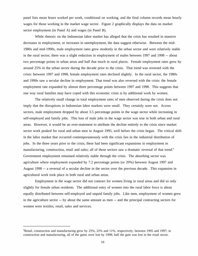
panel lists mean hours worked per week, conditional on working, and the final column records mean hourly

wages for those working in the market wage sector. Figure 2 graphically displays the data on market

sector employment (in Panel A) and wages (in Panel B).

While rhetoric on the Indonesian labor market has alleged that the crisis has resulted in massive

decreases in employment, or increases in unemployment, the data suggest otherwise. Between the mid-

1980s and mid-1990s, male employment rates grew modestly in the urban sector and were relatively stable

in the rural sector; there was a slight reduction in employment of males between 1997 and 1998 -- about

two percentage points in urban areas and half that much in rural places. Female employment rates grew by

around 25% in the urban sector during the decade prior to the crisis. That trend was reversed with the

crisis: between 1997 and 1998, female employment rates declined slightly. In the rural sector, the 1980s

and 1990s saw a secular decline in employment. That trend was also reversed with the crisis: the female

employment rate expanded by almost three percentage points between 1997 and 1998. This suggests that

one way rural families may have coped with this economic crisis is by additional work by women.

The relatively small change in total employment rates of men observed during the crisis does not

imply that the disruptions in Indonesian labor markets were small. They certainly were not. Across

sectors, male employment dropped by about 3.5 percentage points in the wage sector while increasing in

self-employed and family jobs. This loss of male jobs in the wage sector was true in both urban and rural

areas. However, it would be an over-statement to attribute the decline entirely to the crisis since market

sector work peaked for rural and urban men in August 1995, well before the crisis began. The critical shift

in the labor market that occurred contemporaneously with the crisis lies in the industrial distribution of

jobs. In the three years prior to the crisis, there had been significant expansions in employment in

manufacturing, construction, retail and sales; all of these sectors saw a dramatic reversal of that trend.6

Government employment remained relatively stable through the crisis. The absorbing sector was

agriculture where employment expanded by 7.2 percentage points (or 20%) between August 1997 and

August 1998 -- a reversal of a secular decline in the sector over the previous decade. This expansion in

agricultural work took place in both rural and urban areas.

Employment in the wage sector did not contract for women living in rural areas and did so only

slightly for female urban residents. The additional entry of women into the rural labor force is about

equally distributed between self-employed and unpaid family jobs. Like men, employment of women grew

in the agriculture sector -- by about the same amount as men -- and the principal contracting sectors for

women were textiles, retail, sales and services.

6Retail, construction and manufacturing grew by 25%, 22% and 11%, respectively, between 1995 and 1997; inconstruction and manufacturing, all of the gains were lost by 1998; half the gain was lost in the retail sector.

10

Column 5 of each panel reports average hours of work among those working. It has remained

reasonably stable from 1986 through 1997 for all workers. Between 1997 and 1998, however, there was a

substantial cut in hours worked -- about an hour per week in the urban sector and nearly two hours per

week in the rural sector.

Wages

Overall, the crisis has had a small impact on aggregate employment. Wages present a sharp

contrast: the drama of the crisis is reflected in the collapse of real wages of both men and women. This is

vividly displayed in panel B of Figure 2 which places the real wage cuts between 1997 and 1998 in the

context of a substantial rise in real wages during the previous decade. Figure 2 highlights the fact that this

wage growth was especially fast in the three years preceding the crisis, particularly in urban areas. Since

hours of work fell with the crisis, on average, earnings also collapsed during the crisis.

Trends in average wages can mask important changes in the structure of the wage distribution. It

has been argued that the crisis in Indonesia has mostly affected the urban elites (Poppele et al, 1999) which

would be consistent with a large decline in the mean wage but relatively modest changes in real wages of

the poorest. Figure 3 summarizes the entire distribution of wages and how it has changed over time. Non-

parametric estimates of the real wage distribution in the formal wage sector for 1986, 1997, and 1998 are

presented. The figure demonstrates that during 1998 the entire distribution of male and female wages

shifted sharply to the left, relative to 1997. For men, this single year shift in the wage distribution virtually

wiped out all wage gains made since 1986. Among women, the leftward shift in the distribution is large

but they have maintained some of their wage gains since 1986. The key point is that the crisis has affected

the entire wage distribution: between 1997 and 1998, the lowest wage-earners and the highest wage-earners

have all seen real wage cuts, on the order of around 40%.

Sub-group differences

To isolate those sub-groups that have been affected most by the crisis and to assess the statistical

significance of the labor market changes, we have estimated a series of OLS regressions of labor market

outcomes. Since employment and wage trends may be affected by shifting characteristics of the labor

force, the regressions control province of residence, age (specified as splines with knots at 25, 40 and 65

years), education (stratified into five schooling categories), and urban-rural residence. Thus, the estimated

year effects are standardized for changes in the attributes of workers which is potentially important given

the changes in employment rates of women over the last 15 years and the substantial upgrading of the

education of the labor force during this time. The models are estimated separately for men (in the left

panel) and women (in the right panel). Each row of the panel represents a different sample. The first row

includes all respondents; we then stratify by sector of residence, by education of the worker and finally by

age. In each stratified model, variables differentiating members of the group are obviously excluded.

11

Our focus is on changes between 1997 and 1998. The regressions include a calendar year dummy

for every year of the survey with 1997 being omitted. Table 3 reports the coefficient on the 1998 calendar

year control which measures the average (worker attribute standardized) change between 1998 and 1997

and thus highlights the impact of the economic crisis. Variance-covariance matrices are estimated by the

method of the jackknife. Since SAKERNAS contains a large number of observations in each year,

conventional rules of thumb for judging statistical significance are likely to be too lax. We adopt a

Bayesian approach and, following Schwarz (1969), choose a critical value so that the a posteori most likely

model is selected; in the linear regression case, this amounts to choosing a critical value of the test statistic

that is equal to the square root of the logarithm of the number of degrees of freedom multiplied by the

number of restrictions. For a t-test on a particular coefficient, in the first row of the table, the critical value

is 3.66 (for employment rates) and 3.5 (for wages). We adopt this more conservative approach for judging

significance in favor of a classical approach.

Several conclusions about employment can be drawn from the table. First, changes in total

employment rates were relatively modest. Among men, controlling observed characteristics, there was a

1.5 percentage point decline in total labor force participation -- a decline that is concentrated in urban

areas, among more educated workers and among younger workers. There is no significant impact on

employment rates overall for women although, after the crisis, rural women, those with elementary

schooling and older women were more likely to be working while urban, better educated women were less

likely to be working.

There was more action in the sectoral distribution of work. Male employment declined by about

3.7 percentage points in the wage sector. This employment reduction was partially absorbed by the total

labor force withdrawal mentioned above and partly by an increase in self-employed work and, to a lesser

extent, work on the family farm. The reduction in the probability of working in the wage sector was

particularly pronounced among younger men; older male workers seemed to have been better able to find

self-employed jobs which presumably served to cushion the impact of the crisis.

The increases in employment rates among women discussed above are reflected in increases in self-

employment and in unpaid, family work. This is true for rural women, women with elementary schooling

and older women. Running counter to overall trends, female employment in the highest schooling group

actually fell by 4.2 percentage points -- an employment decline that is concentrated in the market wage

sector.

For both men and women, wages fell by almost 40% between 1997 and 1998. Among male

workers, no one has been spared: the wage declines are slightly higher in urban areas, uniformly distributed

across education groups and are largest for the youngest. There are larger, and significant, differences in

the impact on sub-groups of women. The crisis has affected the wages of urban wage workers more,

women in the middle of the education distribution have taken the biggest hit as have younger women. In

12

fact, the only group that has not taken a very large real wage cut are women with wage-earning jobs who

are age 65 to 75 -- a very select (and small) group. In sum, given the magnitude of these wage changes

and the relatively small employment effects, the evidence suggests that short-run labor supply functions are

fairly inelastic in Indonesia.

The statistical models reported in Table 3 provide estimates of only average effects. How were

these real wage declines distributed across lower, middle, and higher wage workers? Table 4 lists the

percent real wage declines that took place in the year of the crisis at selected percentiles of the wage

distribution in the wage sector. To place these wage decreases in the context of the substantial rise in real

wages accompanying economic growth of the previous decade, we also list real wage growth between 1986

and 1997 for the same percentiles. The distributions are arrayed separately by gender and by sector of

residence.

In many ways, the Indonesian economic crisis was an equal opportunity destroyer. Among men,

the substantial fall in real wages during 1998 was only slightly greater among higher wage workers than

lower wage workers. This uniformity contrasts with the more beneficial effects of economic growth on

male wages at the bottom of the wage distribution between 1986 and 1997. As a consequence, the

economic crisis essentially wiped out the previous decade's real wage increases among higher wage men,

but at least left lower wage market sector workers somewhat better off than they were in 1986. This story

of uniform male wage declines during the crisis has to be amended when the data are stratified by location

of employment. Very low wage male workers in urban areas had about a 7% greater wage fall than high

wage urban male workers did. This contrasts with an opposite distributional pattern in rural settings where

there was a tendency for higher wage rural workers to experience slightly higher wage declines. In urban

and especially rural areas, the prior distributional pattern of economic wage growth differentially favored

lower wage workers.

Among female wage earners, the situation was somewhat different as the hardest hit during the

crisis were neither very low nor very high wage earners. Rather, those women who suffered the most were

in the middle of the wage distribution. They experienced wage declines about 10% larger than those at the

bottom or top of the wage distribution. As the accompanying data for 1986-1997 indicates, wages in the

center of the distribution grew the most. The concentration of female wage losses in the middle of the

wage distribution is a consequence of quite different patterns within the urban and rural sectors. All urban

female workers at or below the median experienced about a 10% greater wage loss than urban female

workers above the median. Low wage urban female workers are around median wage earners in the

aggregate distribution and so it is this group that is producing the bulge in the wage shock at the center of

the aggregate female wage distribution. In contrast with low wage workers taking the bigger hit in the

urban sector, among rural woman, wage earners in the upper part of the distribution experienced bigger

wage declines.

13

A key goal of this research centers around the differential impact of the Indonesian economic crisis

on workers in urban and rural labor markets. To gain some insight into this issue, it is not sufficient to

simply estimate mean wage effects within each sector. Mean wages and skills are lower in rural areas so

that an impact of workers of the same skill would be detected at a higher point in the rural wage

distribution than in the urban wage distribution. To see whether economic shocks affect workers of similar

skills differentially in rural and urban labor markets, we first arrayed (within gender) the data by percentiles

in the aggregate 1997 wage distribution. We next found the corresponding percentiles in the urban and

rural wage distribution that matched each aggregate percentile wage. Given that the distribution of urban

wages lies above that of rural wages, these matched urban wages were found at a lower percentile and the

matched rural wages at a higher percentile than the aggregate percentile wage. For each sector of

residence, we then computed the percent change in the wage between 1997 and 1998 yielding a difference

in rural wages and a difference in urban wages at the same real wage. The difference between the rural

wage change and urban wage change is indicative of what happened during the crisis to the urban-rural

wage differential among workers with the same wage in 1997. If wages are equated with skills, this

"difference-in-difference" provides an indicator of the differential impact of the economic shock between

urban and rural labor market at each point in the skill distribution.

Figure 4 plots the (smoothed) estimates of the urban-rural differential in the wage decline during

the year of the shock separately for male and female wage earners across the 1997 wage distribution. The

patterns are remarkably systematic. Among the least skilled men, there was about a 15% decrease in urban

wages relative to the drop in rural wages. This greater relative wage deterioration in urban markets

monotonically declines as we move up the wage (skill) distribution until there is an equal reduction of male

urban and rural wages at the highest wage (skill) levels. The evidence for women essentially parallels that

for men: among the lowest wage (skilled) workers, urban wages declined by between 15 to 20% more than

rural wages but at the top of the wage (skill) distribution, the rural-urban wage differential did not change.

Based on this evidence, we conclude that at least in the formal wage sector, the Indonesia

economic crisis hit unskilled labor markets harder in urban areas than in rural settings. In contrast, there

was little geographic differentiation among the highly skilled. This difference between the change in the

rural-urban wage gap between the lower skilled and higher skilled provides a "difference-in-difference-in-

difference" type of test for the completeness of markets. If markets are complete (or efficient), the

difference-in-difference-in-difference should be zero.7 The fact that it is not provides prima facie evidence

in support of the view that markets are relatively efficient among the higher skilled but that, at least in

times of substantial economic turmoil, markets seem to behave as if they are incomplete among the least

7Prices are probably lower in rural areas. However, uniformly lower prices in rural areas would only alter the locationand not the shape of the curves presented in Figure 4 and so would not affect inferences based on the difference-in-difference-in-difference.

14

skilled. It may reflect barriers to mobility from the urban to rural sector among the least skilled (possibly

because of liquidity constraints) or incomplete information on the part of the least skilled. In either case,

the interpretation is consistent with evidence on the completeness of markets in equilibrium (Pitt and

Rosenzweig, 1986; Benjamin, 1994) but incompleteness in the presence of unanticipated shocks

(Murrugarra, 1998).

Section 4: The Dynamics of the Labor Market Adjustment

The previous section provided a portrait of the Indonesian labor market before and in the midst of

the economic crisis based on SAKERNAS, a time series of cross-sections. While informative, these

portraits are inherently limited in two key dimensions. First, SAKERNAS records income only for workers

in the formal wage sector; this limitation excludes more than half of the labor force. Second, on the

employment side, SAKERNAS is not informative about the dynamics of any labor market adjustments that

took place as workers switched their sectoral or geographic places of work. To address these questions, we

now turn to linked micro data from IFLS2 and IFLS2+. These surveys contain information about

individuals who were interviewed immediately before the onset of the 1998 Indonesian economic crisis and

again a year later.

Market sector and self-employed hourly earnings

It is well-known that collection of income from self-employment in a survey setting is extremely

difficult -- especially, perhaps, in a low-income and substantially agricultural setting like Indonesia.

Difficulties arise, first, because of the need to calculate costs and net those out to compute profit, and,

second, because incomes tend to be volatile over time, often containing an important seasonal component.

The panel feature of IFLS provides some assistance. To the extent that the difficulties in measurement for

a particular individual do not change between 1997 and 1998, these concerns will be somewhat mitigated;

inferences based on changes in self-employment incomes over the period may not be as seriously

contaminated as inferences about levels in incomes.

Figure 5 exploits information on hourly earnings in the market wage and self-employed sector

reported in both IFLS2 and IFLS2+. Non-parametric estimates of the distribution of hourly earnings are

reported for men and women in each sector of employment separately for 1997 and 1998.

Among men and women working in the market wage sector, the IFLS data confirm the general

finding in SAKERNAS that there was a dramatic shift to the left in the distribution of real wages between

1997 and 1998. IFLS indicates there was a similar deterioration in women's income in the self-employed

sector. However, in sharp contrast, real median hourly earnings of self-employed men did not change at all

during the economic crisis. Clearly, inferences about the impact of the crisis based exclusively on market

sector wages (as reported in SAKERNAS) misses part of the picture.

15

The robustness of self-employment hourly earnings may reflect an increase in the amount of capital

used in self-employment businesses (and failure of the respondents to incorporate the costs of capital in

their estimates of profits). This seems unlikely given that credit markets were extremely tight at this time.

It may also reflect increased labor supply of other family members when self-employment income is

derived from family businesses. This is because income from the business is attributed to one family

member and the estimated "hourly" earnings do not take into account the work effort of others. We will

return to this issue below.

The distribution of hourly earnings in self-employment is fatter tailed than the distribution of

wages. In part, this reflects greater error in measurement of self-employed earnings. However, Figure 5

indicates that, relative to 1997, the distribution of hourly earnings in 1998 among self-employed men was

fatter tailed. This increase in variance between the years suggests that some self-employed workers

benefitted from the economic crisis in terms of hourly earnings -- presumably a reflection of increases in

the prices of products they sold -- while others appear to have been all but completely wiped out. In the

rural sector, more than half of self-employed men actually had positive real income changes during the

crisis. Since self-employed men constitute more than half the male work force, any characterizations of the

economic shock in Indonesia using only the wage sector is both incomplete and misleading.

Before comparing wage and employment changes between the SAKERNAS and IFLS, a few

additional adjustments are necessary to make them directly comparable. These adjustments are required

because the IFLS is a panel survey while SAKERNAS is cross-sectional. This distinction mainly affects

labor force patterns for either very young individuals (who are likely to enter the labor market as they age)

or very old individuals (who are likely to exit as they age). To avoid contaminating the comparisons with

these effects of aging, we limit our comparisons in this section to individuals who were between the ages

of 22 and 64 in 1997. Since IFLS2 and IFLS2+ weights are not yet available, a more reliable basis for a

comparison across the two surveys can be obtained from regression models which include as co-variates

controls for the main attributes that determine the sampling weights -- province, rural-urban residence, and

age of respondent. The regression model adjusted impacts reported in Tables 5 and 6 will be less

influenced by different sample weights in the two surveys

Table 5 examines changes in wages in more detail. Drawing on all respondents in IFLS who were

working in either 1997 or 1998, the logarithm of wages has been regressed on an indicator variable for

1998, controlling province of residence, age and education (all measured in 1997). The regressions are

stratified by gender, sector of residence and sector of work. For each regression, the table presents the

coefficient on the 1998 indicator variable which is an estimate of the percent change in real wages between

1997 and 1998 adjusting for inflation and observed worker characteristics. Mean effects, based on OLS

regressions, are reported in the first row. To examine the distribution of changes in wages, quantile

regressions estimates for the 25th, 50th, and 75th percentiles are reported in the following rows; t statistics

16

are calculated by bootstrapping the quantile regressions and jackknifing OLS. (Since the jackknife is a

linear approximation to the bootstrap, the two are asymptotically equivalent in the linear regression case.)

The IFLS percentage wage declines in the market sector are larger than those summarized in the

previous section using SAKERNAS. In part, this reflects differences in the timing of the surveys.

SAKERNAS is conducted in August each year; most of the IFLS interviews were conducted between

August and December in each year. Real wages were relatively constant in 1997. Evidence from

published sources suggests that in 1998 real wages continued to decline from August until December (see,

for example, Papanek and Handoko, 1999). Thus, the IFLS wage changes should be larger than those in

SAKERNAS.8

Figure 5 indicated that self-employment hourly earnings of males were remarkably robust during

the crisis. Table 5 reveals that this is confined to males working in the rural sector. Among urban men

and all women in the IFLS, self-employed hourly earnings declined as much as market sector wages.

Among workers in the market wage sector, percentage declines in wages are fairly uniform across

the distribution with there being a suggestion in the IFLS that the declines are slightly greater for low wage

workers. This same pattern is observed in SAKERNAS. The evidence in support of distributional impacts

of the crisis is stronger among the self employed where declines in hourly earnings are much greater at the

25th percentile than at the 75th percentile indicating that the crisis has taken its greatest toll on the lowest

paid among these workers. It is common to observe that self-employment hourly earnings are more

dispersed than market sector wages; not only is this true in the IFLS but, more significantly, the difference

in dispersion is greater after the crisis than before.

The models have all been re-estimated exploiting the panel design of IFLS more directly by

examining changes in the hourly earnings of each respondent. These models exclude those respondents

who move in or out of the labor force and those who switch sectors. The results are remarkably similar to

those for the fuller sample. There is one striking difference: the decline in hourly earnings at the bottom of

the distribution is greater for rural males in both the market sector and the self-employed sector. This

implies that males who exited the rural labor market were more likely to be from the bottom of the hourly

earnings distribution (or new entrants were more likely to have relatively high hourly earnings) which

suggests there was some upgrading of the rural male labor force.9

8If interviews were randomly allocated over time in IFLS, we could control month of interview and directly compare IFLSwith SAKERNAS. The interviews are not randomly assigned. Because IFLS is a panel survey, interviewers begin inareas that tend to be places migrants move from and end in areas that are destinations for migrants. This reduces the costsof tracking movers. Therefore, we do not attempt to extract any information from the month to month differences withinIFLS.

9The results on wage changes need to be interpreted with the limitations of the price index that has been used in mind.We have relied on the Indonesian government’s official price index which is currently based on prices collected in 44urban centers and a consumption bundle that is fixed for the whole country. Even without an economic shock and its

17

Employment rates and transitions

We return to the employment side of the labor market. Table 6 presents estimates of changes in

sector-specific employment rates between 1997 and 1998 for IFLS and SAKERNAS. The estimates in the

first column are based on OLS regressions of the probability a respondent is working in either year

controlling province of residence, age, education and an indicator variable for 1998. The estimate on the

1998 indicator variable is reported in the first and second row of each panel for SAKERNAS and IFLS,

respectively. The difference between the IFLS and SAKERNAS estimates is reported in the third row.

The remaining three columns are based on regressions of the probability a respondent is working in a

particular sector. The estimates based on IFLS are less precise than SAKERNAS because the IFLS

samples are considerably smaller.

For men, the results parallel those discussed above. There are small changes in labor force

participation rates of urban males with declines in activity in the market sector offset by increases in self-

employment and family work. None of the differences between SAKERNAS and IFLS is significant.

Among rural males, IFLS apparently overstates the decline in participation rates relative to SAKERNAS.

There is one major difference in the results for women. Relative to SAKERNAS, IFLS estimates

significantly larger increases in labor force participation rates during the crisis. The difference is

concentrated in a greater increase in unpaid family work in IFLS. In both urban and rural areas, there is

over a four percentage point increase in the fraction of women working as unpaid family workers during

the economic crisis suggesting that one way households have adapted to the economic shock has been a

significant expansion of work activity by women in family businesses.

In economies such as Indonesia where formal wage sectors co-mingle alongside more traditional

economic activities that often take place within the family unit, measuring work activity in surveys is not

straightforward. SAKERNAS and IFLS take a somewhat different approach to this issue. Both surveys

begin with the same lead-in question on whether, during the week prior to the survey, the respondent was

working.10 In SAKERNAS, those who answer yes' to that question are then asked their type of work.

Family work is one option. The same screener question is asked in IFLS and those who answer yes' are

asked about the type of work. The difference between SAKERNAS and IFLS lies in the treatment of those

accompanying high rates of price inflation, many questions might be raised by this index. First, price changes in ruralareas are obviously excluded from the calculation. Second, the price index is based on the consumption bundle of theaverage household although there is systematic variation in budget shares across the income distribution which impliesthat different price indexes are needed for low, middle and high income households. This is particularly germane in thecontext of the Indonesian crisis since the price of rice, the main staple, rose faster than the general price index. Sincethe share of the budget spent on rice declines with income, the real purchasing power of the poorest likely was reducedmore than the better. Offsetting that effect, households likely substitute towards goods whose relative prices have fallenand away from those whose relative prices have increased.

10Work is defined as an activity for the sake of generating income or helping to generate income that takes up at leastone continuous hour.

18

who answered no' to the lead-in question. In SAKERNAS, they are not asked any more questions about

work. In IFLS, these respondents are asked a follow-up question about whether they had worked for one

hour for pay and, if the response is no, then they are probed by a second follow-up question about whether

the respondent had worked in a family-owned business. Those who answer yes' to either the lead-in or the

two follow-up questions about family business are treated as working and complete the employment

module. This additional probing in IFLS should lead to higher estimates of labor force participation rates

especially among women (which it does). But more important, this additional IFLS probing should make it

easier to detect individuals switching into the family employment sector. If the increase in family work

reported in IFLS arises because of the probing, the follow-up question should have captured more positive

responses in IFLS2+ relative to IFLS2. It did. In IFLS2, 1.8% of female respondents who answer the

question said they worked in a family business; in IFLS2+, 4.1% of women answered affirmatively. This

suggests that many of the people who have entered the family business would not ordinarily consider this

activity as work in some traditional sense. Given this evidence, we are inclined to find the IFLS results on

female family work more credible than those in SAKERNAS.11

To this point, the discussion of labor force activity has been based on cross-sectional evidence.

Table 7 makes use of the repeated observations on individuals in IFLS and tabulates transition rates

between 1997 and 1998 for each type of work activity, conditioning in each case on the respondent’s

activity in 1997. The relatively stable aggregate data on male work activity derived from the cross-section

comparisons masks considerable movement among the sectors and between work and non-work during the

crisis. This churning is particularly prevalent in rural areas where one-third of the men and half the women

changed their sector of work between 1997 and 1998.

Among rural men, the largest net transition that took place was a flow of workers from the formal

market sector to self-employed jobs. 29% of rural men in wage jobs in 1997 moved to the self-employed

sector by 1998. The comparable reverse flow was considerably smaller with only 15% of those in self-

employment in 1997 working in the wage sector in 1998. This net flow of male employment from the

wage to the self-employed sector during 1998 is consistent with our earlier finding that, in rural areas,

hourly earnings of the self-employed decreased much less than of those in wage sector jobs. Among rural

men, there was also a substantial flow from family work into self-employment as more than half of those

rural men who were family workers in 1997 were self-employed by 1998. Note as well that there was

much less movement for men between the self-employed and wage sectors in urban areas where the wage

decreases in each sector were more similar.

11See Korns (1987) who argues that there is evidence in SAKERNAS that self-employment and family employment donot seem to mean the same thing to all interviewers. In addition, he argues that part of the year to year variation in self-employment and family employment in SAKERNAS reflects changes in interviewer quality and training over years.

19

Among women, the most salient pattern is the significant inflows into unpaid family jobs from all

other sectors. In rural areas, the fraction of women working in family jobs increased from 22 to 27%

between 1997 and 1998. Table 7 indicates that these net inflows into family jobs drew women from all

sectors -- those not in the labor force, in the market and in the self-employed sectors. Although this net

inflow into family work also characterized urban women, rates of employment in family jobs remain much

lower there than in rural areas.

We have also examined which type of workers were more mobile between employment sectors.

On this issue, we found that by far the least mobile workers were high wage rural workers in the formal

wage sector. This is particularly clear for men.

Why are these workers so reluctant to change the sector of their employment in spite of the large

decreases in their wages and the possibility of better opportunities in other sectors? The answer appears to

be that they work for the government. In rural areas, two-thirds of men in the upper quartile of the market

wage distribution work for the government. The comparable fraction for women is more than three-

quarters.

Family income

To this point, we have analyzed Indonesian labor markets from the perspective of the individual

worker. But perhaps even more so than in developed countries, the family may represent a more

appropriate unit in which to measure how an economic crisis has impacted the well-being of individuals.

The family represents an important institution that may help smooth out economic shocks among its

members and thereby mitigate some of the risk associated with the crisis. The results obtained thus far

suggest that such adjustments may well be taking place in Indonesia. The increase in female work in family

businesses may be seen as a reaction to the poorer labor market prospects of men during the crisis. If so,

the impact of the crisis on family earnings may be smaller than that on earnings of individual workers.

To examine this issue, Table 8 presents estimates of changes in family earnings between 1997 and

1998.12 As we did for individual earnings, these estimates are presented at the mean, 25th, 50th, and 75th

percentiles as well as the 90th percentile. The left hand panel of Table 8 contains estimates for family

earnings as conventionally measured while the right hand panel augments family earnings to include the

value of own-production of food.

The data summarized in the table indicate that there were considerably different impacts of the

economic crisis on family earnings than that observed for individual hourly earnings (and, therefore, total

earnings since, recall, hours of work declined during the crisis). This is especially clear in the rural areas.

For example, Table 5 indicates that mean wages in the formal sector fell by about 60% in rural areas. The

12Household earnings is calculated as the sum of individual earnings among all members of a household in 1997; thus,we ignore household splits, joins and new entrants. We do this in order to focus on the household unit as it existed in1997, independent of the current location of its members.

20

data in Table 8 indicate that mean conventional family income fell by 37% while mean full family income

declined by 21%. This decline in full family income in rural areas -- while definitely not trivial -- is only

a third of the estimated fall in market wages in rural areas. Evaluated at the mean, the differences between

the impact of the crisis on individual earnings and on family earnings are considerably smaller in urban

areas. In those areas, at the mean, market wages fell by about 55% while full family income fell by 43%.

Table 8 also indicates that the distributional impacts of the crisis appear to be quite different when

measured in terms of family earnings rather than individual earnings. While the evidence was weak that

lower wage workers were differentially impacted by the economic crisis, the evidence for such a

distributional impact is strong in terms of family income -- whether or not the imputed value of own

production is included in the calculation. For example, using conventional family income, in rural areas,

there is a 53% decline at the 25th percentile compared with (an insignificant) 5% drop at the 90th percentile.

This negative gradient is almost as sharp when full family income is used and characterizes both rural and

urban areas.

Why are our estimates of the impact of the Indonesian crisis so different for family income than for

market wages in the formal wage sector? Our analysis points to two principal factors -- the lack of any

significant impact of mean incomes of the self-employed in rural areas and the insurance role of the family

in mitigating the full fury of this economic shock. Table 9 investigates this issue further by summarizing

estimates obtained from a descriptive model of the links between (the logarithm of) family income and the

number of workers in the family.

We have estimated regressions of family income on the number of family members working in the

market, self employed and family business sector in that year; each family contributes two observations and

both income and the number of workers are time-varying. To highlight differences associated with the

crisis, the regressions include a 1998 year effect (reported in the first column of the Table 9). The number

of workers in each sector is interacted with the 1998 indicator variable and those interactive effects are

reported in the odd columns of the table. Column 2, for example, indicates the magnitude of the

correlation between the number of family members in the market sector in 1997 and family income in

1997. Column 3 provides the difference between this correlation and the correlation between the number

of market sector workers in 1998 and income in 1998. The sum of columns 2 and 3 is the correlation

between number of workers in 1998 and income in 1998. Finally, in order to observe any distributional

impacts, quantile models were also estimated.

Three main points emerge from the table. First, not surprisingly, before the crisis, the ranking of

the most important contributions to family income are market wage earners, self-employed and finally

family workers (who contributed not at all on average). Second, the principal impact of the crisis was to

diminish the relative importance of wage earners while simultaneously increasing the importance of the

21

self-employed and family workers. The greater role of family workers is particularly pronounced and, at

the mean, it is significant in the rural sector.

Third, these differences vary dramatically across the income distribution and across sectors of

employment. In urban and rural households, the correlation between family income and the number of

market workers changed little at the bottom of the income distribution but was cut in half at the top. The

reverse is true for self-employed workers in urban areas (and is consistently positive across the entire

income distribution in rural areas). With regard to the number of family workers, the 1998 mean effects

are roughly the same in rural and urban areas (being associated with about a 20% increase in income).

However, the distributional impacts are quite distinct. In urban areas, additional family workers make a

large difference at the top of the income distribution compared to their correlation with family income at

the bottom. For example, we estimate a statistically insignificant negative correlation at the 25th percentile

compared to an extremely positive and significant correlation at the 90th percentile. In urban areas,

therefore, family workers were able to mitigate the impact of the economic crisis among the well-to-do, but

had little impact among the poor. In rural areas, the correlation between income and the number of family

workers was quite different: the distributional impact of family workers in mitigating the crisis was larger

among those in the bottom half of the income distribution.

Recall from the discussion above that one reason we may observe no decline in hourly earnings

among self-employed men in the rural sector is because of increases in the labor supply of family workers.

These results, in combination with those in Tables 5 speak to this issue. The contribution of unpaid family

workers to family income is apparently greatest among the lowest income rural households; however, the

lowest hourly earnings rural males took the biggest hit in terms of a negative earnings shock. This

evidence, in combination with the fact that men have tended to switch out of the market sector into the

self-employed sector in rural Indonesia leads us to conclude that increased family labor supply does not

fully explain the resilience of self-employment hourly earnings of rural men; it appears to be a real

phenomenon and likely reflects the fact that many of these men are net food producers who have benefitted

from the relative increase in the price of food.

Conclusion

It has been argued that the large and abrupt economic decline in Indonesia has resulted in

unemployment on a massive scale. The evidence simply does not support this contention and estimates of

unemployment appear to have been grossly exaggerated. In fact, labor markets in Indonesia appear to be

remarkably flexible.

The drama of the financial crisis lies not in aggregate employment but in real wages, particularly in

the market wage sector. While there have been increases in nominal market sector wages since the onset

of the crisis, these increases have been dwarfed by the rapid increase in prices. According to SAKERNAS,

22

real wages have collapsed by around 40% between August 1997 and August 1998. However, estimation of

the exact magnitude of the decline in real wages is fraught with difficulties, some of which revolve around

computing the appropriate rate of price increases. Inflation has spiralled during this time, there is evidence

of regional heterogeneity in price increases and there have been considerable shifts in relative prices.

Mindful of these concerns, there is evidence in SAKERNAS indicating wage cuts have been greater

in the urban sector, on average. It turns out that this difference is entirely concentrated at the bottom of the

wage distribution where the rural-urban wage differential has declined by around 15%. At the top of the

wage distribution, cuts in real wages are about the same for urban and rural workers. This is prima facie

evidence for flexible (complete) markets among the better skilled but rigidities (incomplete) markets among

those with less skills, at least during times of economic disruption.

These facts emerge in two independent series of household surveys -- SAKERNAS and IFLS.

SAKERNAS, however, does not record information on income from self-employment. IFLS does. Those

data indicate that real hourly earnings of the self-employed in urban areas and of females in rural areas

have declined by at least as much as real market sector wages. In stark contrast, real hourly earnings of

self-employed males in rural areas have remained essentially stable. Given that over half the male work

force are self-employed in Indonesia, conclusions about the effects of the crisis on wages that focus only on

the market wage sector will substantially over-state the magnitude of the crisis.

In fact, Indonesian families have displayed a remarkable capacity for resilience in the face of the

crisis. We estimate that declines in real family incomes are about half the magnitude of the declines in

individual hourly earnings. To be sure, this should not be taken to imply the crisis has not been large and

serious. It has. Our results do suggest, however, that households have adopted strategies that seek to

mitigate the effects of the crisis and that these strategies have been most successful for those at the top of

the income distribution. At the bottom of the income distribution, the crisis has had a devastating impact

on real incomes suggesting that it is the poorest who will likely bear the brunt of any deleterious medium

and longer-term effects of the crisis.

23

References

Benjamin, Dwayne. (1994). "Household composition, labor markets and labor demand: Testing forseparation in agricultural household models,” Econometrica 60(2):287-322.

Cameron, Lisa. (1999). "Indonesia: a quarterly review," Bulletin of Indonesian Economics Studies 35(1),April.

Corsetti, Giancarlo, Paolo Pesenti, and Nouriel Roubini. (1998a). "What caused the Asian currency andfinancial crisis: Part I, A macroeconomic overview," mimeo.

Corsetti, Giancarlo, Paolo Pesenti, and Nouriel Roubini. (1998b). "What caused the Asian currency andfinancial crisis: Part II, The policy debate," mimeo.

Fallon, Peter and Robert E. B. Lucas. (1999). "Economic and financial crises: A survey of the evidence",forthcoming in World Bank Research Observer.

Feridhanusetyawan, T. (1999) "Social Impacts of Indonesia's Economic Crisis: Employment, Income andPoverty Issues" in Social Impacts of the Asian Economic Crisis in Thailand, Indonesia, Malaysiaand the Philippines, Thailand Development Research Institute.

Frankenberg, Elizabeth, Kathleen Beegle, and Duncan Thomas. (1999). "The real costs of the Indonesia'economic crisis: Preliminary findings from the Indonesia Family Life Surveys,” RAND DRU-2064-NIA/NICHD.

Frankenberg, Elizabeth and Duncan Thomas. (2000). "Indonesia Family Life Survey: Study design andresults from Waves 1 and 2," DRU-2238/1, RAND, Santa Monica.

IL0. (1998). "Employment challenges of the Indonesian economic crisis," mimeo, Jakarta.

IMF. (1999). "World Economic Outlook: International financial contagion," World Economic andFinancial Surveys, IMF, Washington, DC.

Korns, Alex. (1987) "Distinguishing Signal from Noise in Labor Force data for Indonesia." DevelopmentStudies Project Research Paper #1. Jakarta: Bappenas/BPS.

Krugman, Paul. (1998). "What happened to Asia," mimeo.

Levinsohn, James, Steven Berry, and Jed Friedman. (1999). “Impacts of the Indonesian economic crisis:Price changes and the Poor,” NBER Working Paper 7194.

Murrugarra, Edmundo. (1998). "Completeness of markets and economic shocks," mimeo, GRADE, Lima.

Radelet, Steven and Jeffrey Sachs. (1998). "The onset of the East Asian financial crisis," mimeo.

Papanek, Gustav and Budiono Sri Handoko. (1999). "The impact on the poor of growth and crisis:Evidence from real wage data," Conference on "The Economic Issues Facing the NewGovernment," Jakarta, August 1999.

Pitt, Mark and Mark Rosenzweig. (1986). In Inderjit Singh, Lynn Squire, and John Strauss (eds.),Agricultural household models: Extensions, applications and policy, Johns Hopkins, Baltimore.

24

Poppele, Jessica, Sudarno Sumarto, and Lant Pritchett. (1999). “Social impacts of the Indonesian crisis:New data and policy implications,” World Bank, SMERU Report, Jakarta.

Schwarz, G. (1978). “Estimating the dimension of a model,” Annals of Statistics 6:461-464.

Thomas, Duncan, James P. Smith, and Elizabeth Frankenberg. (2000). "Lost but not forgotten: Attrition inthe Indonesia Family Life Survey," mimeo, RAND

Thomas, Duncan, Elizabeth Frankenberg, Kathleen Beegle, and Graciela Teruel. (2000). "Householdbudgets, household composition and the crisis in Indonesia: Evidence from longitudinal householdsurvey data," mimeo, RAND

25

Tab

le1:

LA

BO

RM

AR

KE

TC

HA

NG

ES

BE

TW

EE

N19

86,

1997

and

1998

And

repr

esen

tativ

enes

sof

IFL

Spr

ovin

ces

%ch

ange

betw

een

%ch

ange

betw

een

1986

and

1997

1997

and

1998

Prov

ince

s:A

llIF

LS

IFL

S2+

All

IFL

SIF

LS2

+(1

)(2

)(3

)(1

)(2

)(3

)

MA

LE

SW

age

40.3

41.5

42.2

-37.

8-3

8.1

-36.

0U

rban

sect

or36

.237

.137

.3-4

0.6

-40.

9-3

8.6

Rur

alse

ctor

38.2

38.7

39.4

-35.

6-3

5.9

-33.

7

%w

orki

ng-0

.5-0

.7-0

.3-0

.9-1

.1-1

.7in

wag

ese

ctor

7.1

7.1

6.4

-3.0

-2.7

-2.5

self

-em

ploy

ed-3

.3-3

.8-3

.51.

51.

01.

3un

paid

fam

ily-4

.1-4

.0-4

.60.

60.

60.

6

FEM

AL

ES

Wag

e62

.163

.967

.7-3

7.9

-38.

3-3

9.2

Urb

anse

ctor

62.5

64.8

68.7

-41.

3-4

1.8

-43.

3R

ural

sect

or52

.652

.652

.7-3

3.9

-33.

8-3

2.7

%w

orki

ng-2

.3-0

.9-1

.31.

01.

31.

0in

wag

ese

ctor

3.7

3.8

3.8

-0.3

-0.2

-0.2

self

-em

ploy

ed1.

10.

61.

20.

50.

40.

5un

paid

fam

ily-6

.4-5

.5-6

.10.

81.

10.

8

Sour

ce:

SAK

ER

NA

S(1

986-

1998

).IF

LS

prov

ince

sar

eN

orth

Sum

atra

,So

uth

Sum

atra

,W

est

Sum

atra

,L

ampu

ng,

Jaka

rta,

Wes

tJa

va,

Cen

tral

Java

,E

ast

Java

,Y

ogya

kart

a,B

ali,

Wes

tN

usa

Ten

ggar

a,So

uth

Kal

iman

tan,

Sout

hSu

law

esi.

IFL

S2+

prov

ince

sar

eN

orth

Sum

atra

,So

uth

Sum

atra

,Ja

kart

a,W

est

Java

,C

entr

alJa

va,

Wes

tN

usa

Ten

ggar

aan

dSo

uth

Kal

iman

tan.

Wag

ech

ange

sca

lcul

ated

for

thos

ew

hoea

rned

aw

age

inth

em

arke

tw

age

sect

oron

ly;

wag

esm

easu

red

in19

97ru

piah

usin

gB

PSpr

ovin

ce-s

peci

fic

defl

ator

s.A

lles

timat

esw

eigh

ted

bypr

ovin

cew

eigh

ts.

Tab

le2:

EM

PLO

YM

EN

TR

AT

ES

AN

DH

OU

RS

OF

WO

RK

By

gend

er,

sect

orof

resi

denc

ean

dye

ar MA

LE

FEM

AL

ESe

ctor

ofSe

ctor

ofem

ploy

men

tH

ours

Wag

esSe

ctor

ofem

ploy

men

tH

ours

Wag

esre

side

nce

Any

Wag

eSe

lfFa

mily

per

per

Any

Wag

eSe

lfFa

mily

per

per

/Yea

rw

ork

sect

or-e

mp

wkr

wee

kho

urw

ork

sect

or-e

mp

wkr

wee

kho

ur(1

)(2

)(3

)(4

)(5

)(6

)(1

)(2

)(3

)(4

)(5

)(6

)

UR

BA

N19

8666

.339

.124

.82.

546

.611

0930

.514

.210

.95.

443

.368

419

8767

.339

.424

.83.

146

.711

3732

.415

.311

.25.

944

.074

319

8865

.637

.824

.73.

046

.610

1333

.414

.911

.86.

743

.564

519

8965

.237

.924

.33.

047

.710

8931

.715

.310

.75.

744

.171

919

9069

.041

.024

.83.

247

.612

0135

.117

.711

.26.

244

.477

919

9170

.741

.626

.03.

148

.011

8935

.018

.710

.46.

045

.776

419

9269

.940

.626

.62.

747

.612

3335

.618

.411

.16.

144

.584

519

9370

.341

.226

.52.

647

.414

0335

.118

.910

.55.

744

.296

219

9471

.242

.426

.32.

646

.811

8536

.519

.311

.45.

943

.882

919

9572

.143

.926

.32.

047

.114

0634

.319

.610

.93.

843

.710

5319

9671

.843

.226

.81.

846

.515

2236

.719

.413

.04.

342

.511

1619

9771

.942

.627

.22.

146

.815

7837

.719

.812

.55.

442

.912

6019

9869

.738

.828

.32.

545

.811

0437

.018

.812

.25.

941

.983

5

RU

RA

L19

8685

.822

.752

.011

.141

.174

056

.09.

917

.229

.031

.744

619

8785

.924

.150

.011

.841

.069

157

.210

.616

.630

.031

.543

419

8885

.423

.949

.212

.341

.467

158

.411

.116

.630

.732

.239

419

8984

.323

.448

.712

.241

.873

058

.611

.417

.230

.033

.142

919

9086

.523

.451

.211

.841

.572

755

.510

.516

.428

.632

.146

219

9186

.223

.751

.710

.841

.575

954

.510

.116

.228

.132

.153

319

9286

.423

.452

.011

.040

.478

656

.611

.316

.129

.231

.454

519

9385

.725

.151

.29.

540

.886

654

.411

.316

.726

.332

.259

219

9485

.328

.148

.98.

340

.884

253

.611

.118

.923

.633

.056

819

9584

.729

.347

.57.

941

.493

545

.210

.217

.217

.832

.571

019

9685

.427

.252

.25.

939

.510

0753

.011

.023

.818

.130

.770

519

9785

.027

.949

.87.

340

.710

4851

.711

.218

.621

.932

.077

219

9884

.024

.451

.58.

138

.674

554

.611

.319

.923

.430

.555

2

Sour

ce:

SAK

ER

NA

Sus

ing

IFL

S2+

prov

ince

son

ly.

Hou

rly

wag

esin

1997

Rp

defl

ated

with

BPS

prov

ince

-spe

cifi

cpr

ice

indi

ces.

All

rate

san

dm

eans

wei

ghte

d.

Tab

le3:

MA

GN

ITU

DE

OF

EM

PLO

YM

EN

TA

ND

WA

GE

SHO

CK

SR

egre

ssio

nes

timat

esof

diff

eren

cein

year

effe

cts

betw

een

1997

and

1998

By

gend

er,

sect

orof

resi

denc

e,le

vel

ofed

ucat

ion

and

age.

MA

LE

FEM

AL

ESe

ctor

ofem

ploy

men

tW

ages

Sect

orof

empl

oym

ent

Wag

esA

nyW

age

Self

Fam

ilype

rhr

Any

Wag

eSe

lfFa

mily

per

hr(1

)(2

)(3

)(4

)(5

)(1

)(2

)(3

)(4

)(5

)

All

coun

try

-1.4

7-3

.68

1.74

0.47

-38.

460.

81-0

.59

0.50

0.89

-38.

99(5

.70)

(10.

87)

(5.3

1)(2

.81)

(53.

17)

(2.2

4)(2

.26)

(1.8

4)(3

.40)

(33.

42)

Sect

or Urb

an-2

.74

-4.2

11.

080.

39-3

9.99

-1.1

6-1

.32

-0.3

50.

51-4

3.28

(6.9

4)(8

.39)

(2.3

9)(2

.25)

(43.

71)

(2.2

6)(3

.22)

(0.9

9)(1

.99)

(30.

28)

Rur

al-0

.34

-3.2

72.

410.

52-3

6.08

2.51

0.07

1.23

1.20

-31.

20(1

.04)

(7.2

4)(5

.15)

(1.8

8)(3

0.98

)(5

.01)

(0.2

2)(2

.98)

(2.7

0)(1

5.96

)

Edu

catio

nN

one

-0.9

2-3

.05

1.61

0.52

-38.

231.

401.

210.

20-0

.02

-30.

38(0

.72)

(2.3

8)(0

.97)

(0.9

1)(7

.19)

(1.2

6)(1

.74)

(0.2

0)(0

.02)

(6.1

7)E

lem

enta

ry1.

32-1

.64

2.77

0.19

-33.

064.

360.

961.

421.

98-2

5.12

inco

mpl

ete

(2.3

1)(1

.97)

(3.0

5)(0

.51)

(14.

63)

(5.1

8)(1

.77)

(1.9

1)(2

.81)

(7.3

7)E

lem

enta

ry-0

.68

-4.0

22.

730.

61-3

7.56

2.55

0.57

1.17

0.81

-40.

51co

mpl

ete

(1.7

9)(7

.06)

(4.6

8)(1

.94)

(28.

94)

(4.1

5)(1

.39)

(2.4

5)(1

.69)

(18.

09)

JrSe

cond

ary

-2.2

6-3

.20

0.50

0.43

-39.

87-1

.19

-1.5

1-0

.03

0.36

-55.

37(3

.76)

(4.4

2)(0

.73)

(1.0

2)(2

3.17

)(1

.47)

(2.7

2)(0

.06)

(0.6

5)(1

6.64

)Sr

Seco

ndar

y/-3

.40

-4.6

00.

720.

49-3

9.44

-4.1

5-4

.09

-1.2

41.

18-3

9.46

Ter

tiary

(6.1

3)(6

.55)

(1.2

2)(1

.76)

(33.

18)

(4.8

3)(4

.97)

(2.6

4)(2

.88)

(23.

40)

Age

15-2

4-2

.08

-4.0

20.

941.

00-3

8.50

-0.8

6-2

.02

0.37

0.79

-44.

16(3

.05)

(6.8

0)(2

.04)

(2.1

2)(2

3.31

)(1

.33)

(3.9

3)(1

.20)

(1.8

3)(2

2.14

)25

-39

-1.8

9-4

.67

2.26

0.52

-41.

070.

66-0

.11

0.02

0.75

-39.

68(5

.57)

(7.4

3)(3

.68)

(2.2

6)(4

0.40

)(1

.07)

(0.2

4)(0

.05)

(1.6

7)(2

2.69

)40

-64

-1.2

4-2

.74

1.61

-0.1

1-3

3.75

2.27

-0.1

01.

321.

05-3

0.71

(3.7

1)(4

.19)

(2.4

1)(0

.79)

(25.

40)

(3.2

1)(0

.22)

(2.0

0)(1

.83)

(12.

12)

65-7

51.

74-1

.73

3.75

-0.2

8-3

1.57

3.66

1.45

0.97

1.24

-13.

29(1

.50)

(2.1

5)(3

.05)

(0.7

9)(5

.89)

(2.9

8)(2

.63)

(0.9

0)(1

.55)

(1.5

5)

Sour

ce:

SAK

ER

NA

S.B

ased

onO

LS

regr

essi

ons

incl

udin

gin

divi

dual

resp

onde

nts

inal

lye

ars

1986

thro

ugh

1998

resi

dent

inIF

LS2

+pr

ovin

ces.

Reg

ress

ions

cont

rol

prov

ince

ofre

side

nce,

sect

orof

resi

denc

e,ag

ean

ded

ucat

ion

ofre

spon

dent

.Pe

rcen

tage

poin

tch

ange

betw

een

1997

and

1998

repo

rted

for

empl

oym

ent

rate

s;pe

rcen

tage

chan

ges

repo

rted

for

wag

es.

Ass

ocia

ted

tst

atis

ticre

port

edin

pare

nthe

ses

belo

wea

ches

timat

edch

ange

.V

aria

nce-

cova

rian

cem

atri

xes

timat

edby

met

hod

ofja

ckkn

ife.

Est

imat

esfo

ral

lco

untr

y(i

nfi

rst

row

)ba

sed

on63

8,83

6ob

serv

atio

ns(m

ale

empl

oym

ent)

,19

4,37

9ob

serv

atio

ns(m

ale

wag

es)

658,

259

obse

rvat

ions

(fem

ale

empl

oym

ent)

,85

,573

obse

rvat

ions

(fem

ale

wag

es).

Cri

tical

valu

eof

tst

atis

ticfo

rsi

gnif

ican

ceba

sed

onSc

hwar

zcr

iteri

onis

3.66

for

empl

oym

ent

rate

san

d3.

5fo

rw

age

func

tions

inth

ese

case

s.

Table 4: DISTRIBUTION OF WAGE SHOCKSShort-term and longer-term percent wage changes across percentiles of wage distribution

Wage Urban & Rural Urban RuralPctile % change btwn %change btwn %change btwn

86&97 97&98 86&97 97&98 86&97 97&98(1) (2) (1) (2) (1) (2)

MALES10 47.8 -35.9 47.0 -41.6 41.4 -31.630 49.0 -35.9 37.9 -39.9 43.0 -33.050 43.6 -36.8 31.1 -37.3 43.0 -34.370 36.9 -36.7 31.0 -36.4 35.6 -32.990 33.5 -36.4 34.4 -36.3 27.1 -40.195 37.7 -37.4 38.7 -34.0 20.9 -34.0

FEMALES10 50.9 -36.0 68.5 -47.8 34.4 -28.130 69.3 -40.6 81.0 -47.1 49.9 -30.350 81.0 -46.5 71.7 -50.6 55.1 -31.370 77.0 -42.2 50.7 -42.3 58.7 -34.490 61.6 -38.3 51.2 -38.1 59.7 -37.795 53.6 -38.2 49.0 -37.2 47.4 -35.1

Source: SAKERNAS for IFLS2+ provinces. Estimates in column (1) are ln(wage) in 1997 evaluated atappropriate percentile of 1997 wage distribution - ln(wage) in 1986 evaluated at same percentile of 1986wage distribution. Estimate in column (2) is ln(wage) in 1998 - ln(wage) in 1997 evaluated at appropriatepercentiles.

Tab

le5:

AD

JUST

ED

HO

UR

LY

EA

RN

ING

SSH

OC

KS

INM

AR

KE

TA

ND

SEL

F-E

MPL

OY

ED

SEC

TO

RS

Est

imat

edpe

rcen

tage

chan

gein

earn

ings

per

hour

betw

een

1997

and

1998

IFL

Spa

nel

resp

onde

nts

Mal

eFe

mal

eQ

uant

ileU

rban

Rur

alU

rban

Rur

alM

arke

tSe

lfM

arke

tSe

lfM

arke

tSe

lfM

arke

tSe

lf(1

)(2

)(3

)(4

)(5

)(6

)(7

)(8

)

Mea

n-5

3.5

-66.

9-5

7.1

-11.

2-5

8.6

-51.

2-5

8.6

-55.

8[9

.5]

[5.3

][6

.8]

[1.2

][6

.2]

[3.8

][4

.5]

[4.8

]

25%

ile-5

7.5

-89.

0-5

9.7

-24.

9-6

6.5

-76.

7-7

6.1

-63.

3[6

.4]

[5.2

][5

.6]

[1.8

][4

.4]

[3.6

][4

.5]

[3.3

]

50%

ile-4

6.0

-57.

7-4

9.8

-10.

6-5

5.9

-56.

0-6

5.7

-48.

8[6

.7]

[3.4

][3

.6]

[1.1

][5

.2]

[3.7

][4

.4]

[3.1

]

75%

ile-4

0.3

-45.

2-4

6.6

1.2

-54.

0-6

0.8

-48.

1-5

3.6

[6.4

][2

.5]

[5.2

][0

.1]

[5.8

][3

.6]

[2.9

][3

.6]

#ob

s77

339

048

661

132

635

821

045

8

Sour

ce:

IFL

S2an

dIF

LS2

+Pa

nel

resp

onde

nts.

Qua

ntile

regr

essi

onan

dO

LS

regr

essi

ones

timat

esba

sed

onpa

nel

resp

onde

nts

inte

rvie

wed

inIF

LS2

(199

7)an

dIF

LS2

+(1

998)

.E

stim

ated

perc

enta

gedi

ffer

ence

inho

urly

earn

ings

in19

98an

dho

urly

earn

ings

in19

97re

port

edin

tabl

e;[t

stat

istic

s]in

pare

nthe

ses

estim

ated

bym

etho

dof

jack

kinf

e(f

orm

ean)

and

boot

stra

p(f

orqu

antil

es).

Reg

ress

ions

cont

rol

age,

educ

atio

nan

dpr

ovin

ceof

resi

denc

eof

resp

onde

nt.

Table 6: EMPLOYMENT SHOCKSAdjusted Differences Between 1997 and 1998SAKERNAS and IFLS

All Market Self- FamilyWorkers Sector employed Workers

(1) (2) (3) (4)

MALESURBAN

SAKERNAS -2.9 -4.3 1.2 0.2[6.4] [6.9] [2.1] [1.3]

IFLS -1.2 -3.9 1.5 1.2[0.7] [1.6] [0.6] [2.0]

Difference 1.7 0.4 0.3 1.0(IFLS-SAKERNAS) [1.0] [0.2] [0.1] [1.6]

RURALSAKERNAS -0.6 -3.3 2.3 0.4

[2.1] [6.1] [4.1] [1.7]

IFLS -3.4 -0.6 -1.6 -1.3[3.0] [0.3] [0.7] [1.4]

Difference -2.8 2.8 -3.9 1.7[2.4] [1.3] [1.7] [1.8]

FEMALESURBAN

SAKERNAS -0.5 -0.5 -0.5 0.5[0.8] [1.0] [1.0] [1.5]

IFLS 6.6 1.0 1.5 4.2[2.8] [0.5] [0.7] [3.9]

Difference 7.1 1.4 1.9 3.7[2.9] [0.7] [0.9] [3.3]

RURALSAKERNAS 3.1 0.3 1.5 1.3

[5.4] [0.8] [3.0] [2.4]

IFLS 7.0 1.1 0.3 5.7[3.4] [0.8] [0.1] [3.1]

Difference 3.9 0.8 -1.2 4.4[1.8] [0.5] [0.7] [2.3]

Source: SAKERNAS and IFLS. OLS regression estimates of difference between 1997 and 1998;asymptotic t statistics in parentheses estimated by method of jackknife. Regressions include controls forage, education and province of residence.

Tab

le7:

TR

AN

SIT

ION

MA

TR

IXIn

ter-

sect

oral

empl

oym

ent

tran

sitio

nsbe

twee

n19

97an

d19

98

1998

Mal

esFe

mal

es

1997

Mar

ket

Self

-Fa

mily

Not

ΣM

arke

tSe

lf-

Fam

ilyN

otΣ

sect

orem

ploy

edbu

sine

ssw

orki

ngse

ctor

empl

oyed

busi

ness

wor

king

UR

BA

N

Mar

ket

sect

or81

92

857

769

313

22Se

lf-e

mpl

oyed

1479

25

306

689

1723

Fam

ilybu

sine

ss17

5017

171

117

6814

3N

otw

orki

ng22

182

5812

813

574

52

Σ54

322

1310

022

247

4610

0

RU

RA

L

Mar

ket

sect

or63

293

532

539

1424

11Se

lf-e

mpl

oyed

1576

27

586

6020

1427

Fam

ilybu

sine

ss18

5124

75

417

4831

22N

otw

orki

ng29

1912

405

916

2550

40

Σ31

574

810

012

2727

3410

0

Sour

ce:

IFL

S2/2

+pa

nel

resp

onde

nts.

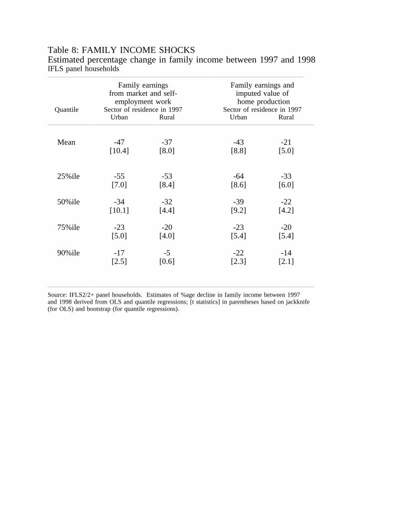
Table 8: FAMILY INCOME SHOCKSEstimated percentage change in family income between 1997 and 1998IFLS panel households

Family earnings Family earnings andfrom market and self- imputed value of

employment work home productionQuantile Sector of residence in 1997 Sector of residence in 1997

Urban Rural Urban Rural

Mean -47 -37 -43 -21[10.4] [8.0] [8.8] [5.0]

25%ile -55 -53 -64 -33[7.0] [8.4] [8.6] [6.0]

50%ile -34 -32 -39 -22[10.1] [4.4] [9.2] [4.2]

75%ile -23 -20 -23 -20[5.0] [4.0] [5.4] [5.4]

90%ile -17 -5 -22 -14[2.5] [0.6] [2.3] [2.1]

Source: IFLS2/2+ panel households. Estimates of %age decline in family income between 1997and 1998 derived from OLS and quantile regressions; [t statistics] in parentheses based on jackknife(for OLS) and bootstrap (for quantile regressions).

Table 9: FAMILY INCOME SHOCKS AND FAMILY EMPLOYMENTCorrelations between number of family members employed in each sector and family incomeMain effects and interactions with control for 1998IFLS panel households

# workers in each year: market sector self employment unpaid family busYr=1998 *1998 *1998 *1998

(1) (2) (3) (4) (5) (6) (7)

URBANMean -50.9 44.1 -5.8 24.4 3.3 -6.3 22.5

[4.0] [11.0] [0.9] [5.2] [0.4] [0.6] [1.2]

25%ile -73.3 44.6 1.6 22.3 -2.7 4.0 -8.1[3.0] [7.5] [0.1] [3.5] [0.3] [0.3] [0.4]

50%ile -36.7 41.5 0.7 20.2 -6.8 -3.4 2.8[2.3] [9.6] [0.1] [3.5] [0.6] [0.3] [0.2]

75%ile -19.5 44.6 -10.3 24.5 3.7 -11.6 26.1[1.3] [10.9] [1.6] [3.6] [0.3] [0.7] [1.0]

90%ile -12.3 36.5 -15.1 24.7 18.4 -18.2 92.8[0.5] [5.8] [1.4] [2.4] [1.2] [0.6] [2.0]

RURALMean -53.7 53.4 -14.1 19.4 10.8 -5.6 27.6

[3.5] [8.9] [1.6] [3.2] [1.2] [0.9] [2.9]

25%ile -85.3 58.8 -5.1 19.7 10.1 -6.2 33.6[3.9] [5.9] [0.4] [2.4] [0.7] [0.8] [2.9]

50%ile -40.8 54.1 -18.7 19.0 2.0 -1.6 21.3[1.7] [8.8] [1.9] [2.8] [0.2] [0.2] [1.7]

75%ile -33.9 41.6 -10.6 11.7 11.9 -1.9 14.7[2.2] [5.4] [1.1] [1.5] [1.1] [0.2] [1.4]

90%ile -8.2 42.4 -27.4 18.4 9.3 -7.3 14.2[0.3] [3.6] [1.5] [1.9] [0.6] [1.1] [0.8]

Source: IFLS2/2+ panel households. Estimates based on regressions of ln(family income) on indicator variable for1998 (column 1), number of workers in market sector, self employment and family work in each year (even columns)plus interaction between the number of workers in each sector and 1998 indicator variable (odd columns). [t statistics]in parentheses based on jackknife for OLS and bootstrap for quantile regressions.