ECONOMIC GROWTH CENTERYALE UNIVERSITY

P.O. Box 208269New Haven, CT 06520-8269

http://www.econ.yale.edu/~egcenter/

CENTER DISCUSSION PAPER NO. 868

WAGE RENTALS FOR REPRODUCIBLE HUMAN CAPITAL: EVIDENCE FROM GHANA AND THE IVORY COAST

T. Paul SchultzYale University

September 2003

Notes: Center Discussion Papers are preliminary materials circulated to stimulate discussions and criticalcomments.

Permission to analyze the LSMS data from Côte d'Ivoire and Ghana in preparing a conceptualsurvey of human resource programs for the World Bank is appreciated. Also, I appreciate theprogramming assistance of Paul McGuire, the comments of Michael Boozer, William Dow, JohnMaluccio, Tomas Philipson, Debby Reed, Duncan Thomas, and those of the participants at theStanford Development Workshop. The support of the Rockefeller Foundation is acknowledgedwith pleasure. Only the author is responsible for errors. paul.schultz@yale.edu

This paper can be downloaded without charge from the Social Science Research Network electroniclibrary at: http://ssrn.com/abstract=441942

An index to papers in the Economic Growth Center Discussion Paper Series is located at: http://www.econ.yale.edu/~egcenter/research.htm

Wage Rentals for Reproducible Human Capital:

Evidence from Ghana and the Ivory Coast

T. Paul SchultzYale University

Abstract

Education, child nutrition, adult health/nutrition, and labor mobility are critical factors inachieving recent sustained growth in factor productivity. To compare the contribution of these fourhuman capital inputs, an expanded specification of the wage function is estimated from household(LSMS) surveys of The Ivory Coast and Ghana. Specification tests assess whether the human capitalinputs are exogenous, and instrumental variable techniques are used to estimate the wage function.Smaller panels from the Ivory Coast imply the magnitude of measurement error in the human capitalinputs and provide more efficient instruments to estimate the wage equation. The conclusion emergesthat weight-for-height and height are endogenous, particularly prone to measurement error, andheterogeneous in their effects on wages. Overall returns to these four forms of human capital are similarwithin each country for men and women, but education and migration returns are higher in the morerapidly growing Ivory Coast, and the wage effects of child nutrition proxied by height are greater inpoorer, more malnourished Ghana.

Keywords: Endogenous Human Capital Returns, Health, Migration, Schooling, Africa, PhysicalStature.

JEL codes: J24, I12, O15, J31

1

1. INTRODUCTION

Schooling, height, weight-for-height, and migration are attributes of workers associated with their current

productivity. These forms of worker heterogeneity are to some degree reproducible: schooling and migration are created

by well-described processes, whereas height and weight-for-height are formed by the biological process of human growth,

in which the inputs of nutritional intakes, protection from exposure to disease, health care, and activity levels combine to

exert a net cumulative effect on the individual's realization of their genetic potential. The impact of height and weight-for-

height on labor productivity and well-being have been extensively documented by economic historians (Fogel, 1994,

Steckel, 1995), and more recently studied in contemporary random surveys from low-income populations (Strauss and

Thomas, 1995). These worker attributes are viewed here as indicators of human capital because they can be augmented by

social or private investments, but they also vary across individuals because of genetic and environmental factors that are

not controlled by the individual, family, or society. This paper estimates the productive payoff to the formation of these

four human capital stocks in two low-income countries.1 Because the cost of creating these stocks has not been accounted

for, only estimates of the wage rental values of these stocks are offered here and not internal rates of return. Several

questions are addressed.

First, how important for labor productivity is each of these four dimensions of worker heterogeneity considered

jointly, for men and women separately, in two Sub-Saharan African countries where the conditions of health and nutrition

are relatively poor?2 Second, do the wage payoffs to forms of human capital change when one allows for human capital

stocks to be endogenous, heterogeneous, and measured with random error. Finally, how do these forms of human capital

interact in their determination of worker productive capacity; can complementarity between forms of human capital

(interactions) be distinguished from changing "returns to scale."

In Section 2, a simple framework is outlined for guiding the estimation of an extended wage function that

includes several, possibly endogenous, heterogeneous, and measured with error, human capital stocks. The data are

described in Section 3. Empirical specification issues are discussed further in Section 4. Sections 5 and 6 report the

estimates for cross sectional surveys from the Ivory Coast and Ghana. Then in Section 7, for a smaller two-year panel from

adjacent years of the Ivory Coast surveys, measurement error is quantified and alternative estimates of wage functions are

compared. Section 8 presents flexible form estimates to assess non-linearities, and Section 9 reconsiders the gender wage

gap in terms of the human capital inputs. Section 10 summarizes the new evidence and suggests how further research

might resolve some of the outstanding questions.

2

2. THE DEMAND FOR HUMAN CAPITAL AND THE WAGE FUNCTION

Household demand for human capital is represented as a derived demand for the services of these capital stocks,

which is a function of the prices of inputs to produce these stocks, the discounted value of the increased output they

produce, local public services and relevant conditions, as well as the credit available to parents, and the parents' own

endowments. Four forms of human capital are considered here as an input, I ij , where i refers to the individual and j to

the type of human capital: H for adult height as an indicator of childhood nutritional status (Faulkner and Tanner, 1986;

Behrman, 1993); E for years of education (Becker, 1993; Mincer, 1974; Griliches, 1977); B for body-mass-index (BMI

= weight in kilograms divided by height in meters squared) as an indicator of adult nutritional status and current health

(Fogel, 1994; Steckel, 1995; Strauss and Thomas, 1995) , and M for whether the individual has migrated from the region

of birth (Schultz, 1982) :

,ij j i j i ijI a Y Xβ ε= + + , , ,j H E B M= (1)

where the critical distinction is between Y that affects the demand for human capital partly through its impact on wage

structures which provide the labor market incentive to invest in human capital, as well as through other possible channels,

and X that affects the demand for human capital without modifying the structure of expected wage opportunities. For

example, the price of an input used in the production of the human capital might be specified as a variable in X, but would

not affect the local wage returns to human capital, such as the local price of food or nutrients (Strauss, 1986), whereas

residing in a rural area might be specified to Y which could capture the higher cost of obtaining health care in a rural area

and also be associated with different wage returns from human capital in these areas. The parameters of behavioral demand

and human capital production technology are not separately identified in these reduced-form parameters, α and β, that are

estimated in (1). The errors, ε ij , are assumed uncorrelated with Y and X.

A standard semi-logarithmic linear approximation of the wage function is expanded here to include the four

noted human capital inputs and the vector of exogenous variables (Y) that additively affect the logarithm of wages:3

4

i j ij i ij l

w I y vγ δ=

= + +∑ (2)

The human capital inputs are exogenous in the wage function if the wage error is uncorrelated with the errors in

the human capital demand functions, or the covariance ),( iji εν = 0, for j = 1, ..., 4. If this cross equation error

3

covariance is not zero for some j , then the jth form of human capital is endogenous and ordinary least squares (OLS)

estimates of the wage equation are biased.

To test for the exogeneity of the human capital inputs, the wage function parameters must be identified, possibly

by an exclusion restriction, represented by the vector of X instruments in the human capital demand equation (1). A

significant difference between the OLS estimates, consistent even if the inputs are exogenous, and instrumental variable

(IV) estimates, consistent even if the inputs are endogenous, defines the standard specification test (Hausman, 1978). One

way to specify appropriate instruments for this problem is to explore in more detail the probable sources of human capital

input endogeneity.

One form of endogeneity could arise if there are exogenous unobserved differences across individuals in their

original endowments, and these endowments could influence how parents and children invest in human capital, in possibly

a compensatory or complementary manner. Examples of this type could be "ability" affecting the demand for education

(Willis and Rosen, 1979), and "frailty" affecting the demand for health inputs (Rosenzweig and Schultz, 1983). These

forms of innate heterogeneity that are not observed by the researcher could cause a correlation between the human capital

inputs and the error in the wage function and thereby lead to biased OLS estimates of the wage function.4 There are two

approaches to this problem. Either measure the omitted variable, e.g., genetic ability, and include it in the wage function,

or choose an instrument for the input such as market prices or random temporal and spatial shocks, e.g., rainfall, that are

expected to influence human capital demands but not otherwise affect subsequent wage opportunities of the individual.

A second type of misspecification arises when two inputs are aggregated that have different productive effects on

wages. If the instruments are more strongly correlated with one of the two inputs, the specification test may reject the

exogeneity of the aggregated input, because the IV estimate will predict one component better than the other. For example,

height across a birth cohort may be largely determined by the genetic capacities or genotype distributed across the

population at conception, although its expression may be modified by subsequent resource allocations. Individual

nutritional intakes, exposures to disease, treatment of these diseases, and variation in other environmental burdens

determine net nutritional status, which then facilitates or stunts the expression of genetic potential for adult height. As a

readily measured and objective index of healthiness, productivity, and well being, height encompasses a wide range of

biological characteristics that are otherwise difficult to quantify and decompose (Faulkner and Tanner, 1986). Deviations

of height from genetic potential are particularly sensitive to early childhood living conditions (Martorell and Habicht,

1986). The two components (genotype and phenotype) of height are equally relevant to economic or welfare outcomes. In

4

a population that is closed to emigration or immigration and does not experience change in its mix of biological groups

(e.g., by race), changes in average height over time may be plausibly attributed to changes in reproducible human capital

investments, or changes in disease environments, or both. Yet, in the cross section, the fraction of the variance observed in

height that can be explained by socioeconomic endowments and constraints may have a larger (or smaller) effect on

productivity than the fraction of the variance in height that is not explained by socioeconomic variables and is presumably

more likely to arise from genetic variability.

Aggregating these different sources of variation in height could lead to misleading inferences on the relative

importance of augmenting height by lowering food prices or reducing the virulence of disease. This form of aggregation

bias could also lead to the rejection of the exogeneity of height according to the standard Hausman-Wu specification test,

if the X includes only socioeconomic endowments and constraints. The origin and interpretation of this type of aggregation

bias differs from the first type of heterogeneity bias. Confronted by human capital inputs in the cross section with two such

components, as with height and perhaps BMI, selecting instruments that determine behavioral demands for human capital

and that are not correlated with genotypic variability in these inputs should improve estimates of the effect of the

reproducible component in human capital. Those characteristics in the population which are more likely to be related to

relevant genetic groups, e.g., race, language, or birthplace, may be included in the vector of control variables, Y, that enters

both the wage and the human capital demand functions, in order to avoid relying on inter-group genetic variation to

identify the wage effects of the reproducible component of human capital.5

Errors in measurement of the human capital inputs could also explain why the apparent wage effects of the

inputs when directly estimated by OLS are downwardly biased compared with the IV estimates. This source of bias could

be detected by the specification test and be corrected by instrumental variable estimation methods. If the measurement

errors were random, due to, say, coding errors and numerical rounding mistakes, and were independent from one

observation to the next for the same individual, it might be directly assessed in a panel. Averaging two periods, for

example, would reduce such white noise and attenuate the bias due to this source of error. The matched observation on the

same human capital input from another round of the survey could provide a relatively efficient instrument for this round's

error-measured input observation, potentially correcting for this source of bias.

Thus, three alternative models could account for a specification test that rejects the exogeneity of human capital

inputs. The bias due to omitted variables and errors-in-measurement could plausibly introduce off-setting effects on a

5

human capital coefficient in a wage equation, such as with education (Griliches, 1977; Lam and Schoeni, 1993). These off-

setting sources of bias could weaken the power of the specification test to reject exogeneity.

The functional form of the wage equation may also be more complicated than expressed in (2). Diminishing (or

increasing) returns to the individual's accumulation of each form of human capital is often plausible from a biological or

economic perspective. The empirical specification of the wage function should flexibly allow for this possibility. For

example, the effect of nutrition on physical growth and adult productivity is expected to be subject to diminishing returns

(Strauss, 1986; Strauss and Thomas, 1995). The proportionate increase in wages associated with a specific increase in

nutrition may be greater for those who are especially malnourished. This nonlinearity in returns to nutrition has buttressed

the efficiency wage hypothesis (Bliss and Stern, 1978) and motivated theories of malnutrition and inefficiency due to

market failure (Dasgupta, 1993; Foster and Rosenzweig, 1993). The proportionate increase in wages associated with an

additional year of schooling is often reported to be smaller at higher levels of schooling (Psacharopoulos, 1994). Although

economists are accustomed to this empirical regularity suggesting diminishing returns to "scale" of human capital

investments (Becker, 1993), the opposite pattern of increasing returns to education is also documented today, when

bureaucratic bottlenecks or perhaps credit constraints hinder the economically efficient expansion of intermediate or higher

levels of schooling.6 Nonetheless, the predominant pattern, if not a rule, is for human capital returns to be higher at lower

levels of investments. Consequently, investments in human capital could be equilibrating and if targeted to the poor could

reduce economic inequality and also promote efficient growth.

Finally, human capital inputs may technically substitute or complement each other in their effect on labor

productivity, depending perhaps on the nature of tasks the individual performs in the labor market. For example, weight

may become less valuable for increasing the productivity of workers as they become more educated and qualify for white-

collar jobs where physical strength and endurance are of less value. Existing empirical evidence on interactions between

types of human capital does not consider human capital inputs as potentially endogenous or subject to variable returns to

scale. Reported interactions that treat human capital as exogenous may not, therefore, serve as a reliable guide to the

importance, or even sign, of the technical input interactions between endogenous forms of human capital.7

The wage function should be estimated, therefore, in a flexible form that allows for nonlinearity and interactions

in addition to the multiplicative form implied by the standard semi-logarithmic wage function (Mincer, 1974).

Consequently, a second-order approximation of the log wage function will be considered later in Section 8 (Fuss and

McFadden, 1978), with the human capital inputs tested jointly for their exogeneity.8

6

. + Y + I + II + I = w ii2ijj

3

j=1ikijjk

4

1+j=k

4

j=1ijj

4

j=1i νδθηγ ∑∑∑∑ (3)

Note that the squared effect of migration human capital is not estimated because it is measured as a dichotomous variable,

equal to 1 if the individual has migrated away from their birthplace and zero otherwise. This more flexible form of the

wage function (3) is obviously more difficult to estimate precisely because 13 input coefficients are now estimated

(compared with 4 in (2)), and these additional variables are highly correlated with each other by construction. This

multicollinearity problem is more serious if some of the input variables are subsequently assumed endogenous and must

then be predicted on the basis of the same vector of instrumental variables (X) . Practically, it should be expected that in

this context only a few of the quadratic and interaction terms will prove statistically significant in modest-sized samples of

only a few thousand individuals. Thus, a more parsimonious linearized specification is likely to be accepted strictly on

grounds of parsimony and statistical fit (Rosenzweig and Schultz, 1983). Nonetheless, empirical evidence that certain

higher-order terms in the expanded wage function (3) are statistically significant should not be entirely discounted because

all such terms are not jointly significant. If any of these higher order terms are empirically decisive, they could increase the

precision of inferences on how public and private expenditures are best deployed to increase labor productivity.

Correlations may be expected between different forms of human capital across individuals, and the greater the magnitude

of this intercorrelation of inputs the more difficult it may be to estimate the productive payoff to each input separately.9

Another problem in estimating the wage equation is the unrepresentativeness of the sample of individuals who

report wages. To correct this potential sample selection bias, variables must be observed that are arguments in the sample

selection decision rule that are theoretically restricted from affecting the market wage equation (Heckman, 1979).

Conditional on the assumption that physical wealth and non-earned income identify the probit selection model, the

correlation of the errors between the wage earner participation probit equation and the log wage equation are in the

samples considered here generally insignificant. Estimated returns to schooling or adult health are robust to these

corrections for sample selection bias (Schultz, 1993; Schultz and Tansel, 1997).10 Sample selection bias will therefore be

neglected here.

7

3. CHARACTERISTICS OF THE SAMPLES

Table 1 reports the average levels of the four indicators of human capital stocks for men and women from the

Ivory Coast and Ghana, by age, according to the Living Standards Measurement Surveys circa 1985-1989.11 Some

individuals in the youngest age group, 15 to 19, are continuing to invest in education, and individuals in this age group are

still growing toward their adult stature of height and BMI. Migration, because it is a cumulative measure of having ever

migrated since birth, increases with age within a birth cohort, but may not increase across age groups in a cross section if

mobility has been increasing over time for more recent birth cohorts.

Years of schooling completed began to increase sharply at least a decade earlier in Ghana than in the Ivory Coast.

Men's education in the Ivory Coast increased in three decades nearly seven fold from .9 years for men age 50-65 to 6.0 for

those age 20-29. In Ghana men's education more than doubled in this period from 3.6 to 8.3 years.12 Women age 50-65

have only one-seventh as many years of education as do men in The Ivory Coast, whereas women 50-65 in Ghana have

one-fourth as much education as do men. In the Ivory Coast women in the age group 20-29, who received their education

approximately during the 1970s, have 69 percent as many years of schooling as do men, and women this age in Ghana

have four-fifths as many years of education as do men. Women clearly receive substantially less education than do men in

these two populations. Although this gender gap is closing, it still remains absolutely large at the secondary school level,

particularly in The Ivory Coast (Schultz, 1993).

The indicator of migration peaks for women in The Ivory Coast in the ages 20-29 and for men at ages 30-39. In

Ghana, where economic growth started earlier in this century but has been slower since the mid-1960s than in The Ivory

Coast, migration is less frequent and more uniform across ages.

Height for males in the Ivory Coast shows an increase from 1.67 meters among the oldest group, age 50-65, to

1.71 among those age 20-29. This four-centimeter increase is larger than the two-centimeter increase observed among

males in Ghana. Women in the Ivory Coast report a height gain of 3 centimeters between the same age groups, whereas the

gain for women in Ghana is only one centimeter. In these three decades real GNP per capita increased about 70 percent in

Ghana and 316 percent in The Ivory Coast (World Bank, 1991). These gains in height could plausibly reflect the improved

nutritional status of youth maturing during the 1970s compared with those growing up during the 1940s and 1950s. As of

1990, 36 percent of the children under age 5 are still malnourished in Ghana, whereas only 12 percent are estimated to be

malnourished in the Ivory Coast (World Bank, 1991).

8

The time trend in height across birth cohorts can also be estimated with greater precision at the individual level,

by regressing height on age while controlling for membership in groups that may share a genetic component and which

may have changed their proportions in the population over time, such as ethnic/language/religion and birthplace groups

(Appendix Table A-1). Restricting the sample to men and women ages 20 to 60 to exclude most of those who are still

growing or the elderly who may be shrinking, the ordinary least squares linear trend estimates imply a rate of growth in

height of 0.52 cm per decade in Ghana for women (t=6.97) and 0.48 cm for men (t=5.18), and about one centimeter per

decade for men and women in the Ivory Coast (1.1 cm (t=11.8) and .99 cm (t=13.7), respectively). These estimates are

within the standard growth increments experienced during the second half of the 20th century of between 0.3-3 cm per

decade (e.g. Cole 2003).13

Because the body-mass-index often increases with age, the tendency for BMI to peak for men and women in the

age group 30-39, as shown in Table 1, does not clarify whether there has been an improvement over time in BMI in either

country across birth cohorts. Controls for age differences in BMI, therefore, should be interpreted with caution, for they

could capture both aging and changes over time in nutritional status.

The demand determinants (eq. 1) and the productive consequences (eq. 2) of the four human capital stocks are

estimated in the next section for persons age 20 to 60, allowing for variation across the four age groups distinguished in

Table 1 by including three dummy age group variables.

4. EMPIRICAL SPECIFICATION OF THE MODEL

If the human capital stock variables are measured with error, biologically heterogeneous, or are affected by

unobserved characteristics of individuals, families, or communities that also affect wages, ordinary least squares (OLS)

estimates of the wage equation (2) will be biased. To obtain consistent estimates in these circumstances instrumental

variable methods may be used, in which the instruments are sufficiently correlated with the human capital variables, but

strictly not correlated with the wage equation error. Conditional on the other variables included in the wage function (Y),

good instruments (X) should then explain a statistically significant part of the variation in the demand for the human

capital variables (Bound et al, 1995). The second criterion of a good instrument is that it not be information an employer

would know and plausibly use to determine a potential worker's wage offer, while it might motivate the prior acquisition

of any of the four forms of human capital analyzed here. 14

First, there are productive characteristics of the worker that could be included in both the wage function and in

the human capital demand function (Y): The age and ethnic/language group, rural/urban residence, region of birthplace,

9

average annual rainfall, and whether the interview occurred during the biannual rainy (malarial) season in the north or

south. In West Africa height and weight, as well as education and migration differ by ethnic group, and ethnicity may be

correlated with other omitted forms of human capital and even genetic variability that could possibly influence worker

productivity. The twice-a-year rainy season is associated with increased malaria and other water-borne diseases, which

temporarily disable or reduce the productivity of many adults e.g., because of diarrhea. The derived demands for labor in

agriculture are also affected by season and vary by climatic region, and should be expected to affect wages.

The instruments that are assumed to only affect the demand for human capital inputs (X) and identify the wage

equation include: (1) community health infrastructure, water and sanitation conditions, the distance to a doctor and clinic,

and distances to various school facilities and a permanent market; (2) eight to eleven community prices of food items; and

(3) father and mother education and whether they worked in agriculture. The hourly wage rate, inclusive of income in

kind, is deflated by a regional price deflator to approximate a real wage (Schultz and Tansel, 1993). Consequently, the

relative prices of food staples in the community should capture the relative cost of nutrition that might influence current

nutrition and BMI in particular (Strauss, 1986; Thomas and Strauss, 1996). Increasing distance to middle and secondary

schools should discourage schooling by increasing its private cost. Community health infrastructure and access to medical

care are expected to influence the prevalence of diseases and affect net nutritional status, as proxied by height and BMI.

However, many individuals have moved from their birthplace and human capital investments such as height and

schooling, are partly determined by local conditions as a young child. Therefore, for migrants, local condition variables are

set to the average conditions prevailing for respondents still living in the regions where the migrants were born. Because

the surveys do not ask migrants whether they were born in a rural or urban area, it is assumed that they were born in rural

areas, except for those reporting their birthplace as the capital city. Local conditions will have changed, moreover, since

the respondent was a child. The statistical significance of these contemporary instruments in explaining past human capital

inputs might thus be attenuated among older respondents.15

The birthplace region, of which eleven are distinguished in each country, may itself proxy unobserved regional

variation in schooling and health facilities, and may contribute to migration, given the different regional levels of

development and wage opportunities. Wages may differ by birthplace region for reasons other than the individual's

accumulation of the four observed stocks of human capital, and that is allowed for within the model's specification by

including birthplace in the wage equation. Parent education and occupation are assumed to influence the respondent's

investment by means of changing the four observed forms of human capital. If parents also affect the formation of other

10

unobserved skills and traits of children that enhance their offspring's productivity as adult workers, the parent

education/occupation may be an invalid instrument. One approach to detect this problem is to also include the parent

characteristics in the wage function directly, or assign them to Y rather than X (Lam and Schoeni, 1993). This approach

may also bias down the estimated wage effects of the human capital inputs (Griliches, 1977), but in the case at hand,

conditioning wages on parent characteristics does not significantly add to the explanatory power of the wage function.16

5. ESTIMATES OF THE EXTENDED WAGE FUNCTION

Different forms of human capital tend to be positively correlated with each other. In both countries and for both

men and women, 20 out of the possible 24 correlations between the four human capital variables are positive and

significant at the 1 percent level (Appendix Table A-2). An exception is BMI and height, in which BMI is constructed to

be approximately orthogonal with height, as seen in The Ivory Coast, in order to facilitate multivariate studies of the joint

effect of height and BMI on health outcomes (Fogel, 1994).

All of the forms of human capital are individually positively correlated with the log hourly wage variable in each

of the 16 cases at a significance level exceeding .01 percent (Table A-2). Consequently, the estimated effect of any of the

human capital variables on the log of hourly wage rate is likely to be upward biased, if other human capital variables are

omitted from the wage function (Griliches, 1977). The nature of the bias could be complicated by possible nonlinear

effects of the human capital inputs on the log wage and interactions with other variables. Indeed, the relationship between

BMI and health is not only nonlinear, it appears to be non-monotonic; health outcomes such as mortality, chronic

morbidity, or nonparticipation in the labor force among elderly men increases with BMI in excess of about 28 (Fogel,

1994; Costa, 1996).17 The effect of years of education on log wages is often noted to be decreasing with scale, although

instances of education returns increasing are also documented (Schultz, 1993). It is thus an empirical issue of how much

estimates of the wage returns to education may be biased (presumably upward) by the omission of other forms of human

capital in the wage function.

Table 2 reports estimates of the linear specification of the log wage equation for only the human capital

coefficients, in which controls (Y) are also included. Columns (1) through (4) report ordinary least squares (OLS) estimates

based on the assumption that the human capital inputs are exogenous, homogeneous, and measured without error. Adding

sequentially migration, BMI, and height, according to their average correlations with education (Table A-2), to the more

conventional wage equation reduces the initial estimate of the private returns on education (Cols. (1) through (4)) as was

expected. If these human capital stocks are exogenous and measured without error the estimates of the wage returns to

11

education appear to be biased upward by about 5 to 15 percent by the omission of these three other forms of human

capital. Only height in the Ivory Coast among women is not statistically significant in the full multivariate exogenous

specification of the wage function (4), just as it was least significant in the simple correlations with wages (Table A-2).

According to the OLS estimates in Column (4), a year of completed schooling has an average effect of increasing

wages by 11 percent for men and 7 percent for women in the Ivory Coast and 4.4 percent for men and 3.8 percent for

women in Ghana. This larger return to education in the Ivory Coast than in Ghana could be attributed to the larger initial

supply of educated workers in Ghana or to the slower economic growth in Ghana since independence that may have

depressed the relative derived demands for more skilled workers. Migration from region of birth is associated with a larger

gain of 72-89 percent in wages in The Ivory Coast than the 35-53 percent in Ghana, probably related to the greater

integration of the national labor market in Ghana than in the Ivory Coast and the correspondingly larger wage differentials

favoring Abidjan than those prevailing in Accra. The cultural-political barriers to movement across tribal regions may

inhibit interregional migration to a greater extent in The Ivory Coast than in Ghana. Change in a unit of BMI is associated

with similar percentage changes in wages in both countries, 4.2 to 6.1 percent, but sample variability in BMI is greater

among women than men, with standard deviations about 4.2 versus 2.6, respectively (Appendix Table A-1). The

association between wages and height is stronger in Ghana than in the Ivory Coast suggesting that malnutrition among

children is more often a binding constraint on adult height in Ghana. An individual who is one centimeter taller (the

standard deviation is 6-7 cm.) receives in Ghana a wage that is 1.3 to 1.5 percent higher, whereas taller men in the Ivory

Coast receive a wage that is .95 percent higher per centimeter, and women receive a wage that is .25 percent higher. These

OLS estimates reinforce the standard view that education is the dominant reproducible form of human capital, with

migration second, followed by significant but relatively small effects related to height and weight-for-height. However, the

question arises how might these estimates be biased by the econometric problems discussed earlier?

6. ENDOGENOUS DEMANDS FOR HUMAN CAPITAL INPUTS

Table 3 summarizes in Column (1) the overall explanatory power of the first-stage estimates of the human capital

input equations, in Column (2) the increment to the R2 contributed by only the identifying instruments, and in Column (3)

the F ratio test of their joint statistical significance. In addition to the 22 identifying instrumental variables in the Ivory

Coast and 30 in Ghana (Table A-1), interactions of the instruments with the controls and quadratic terms in parent

education are also included as identifying variables (48 variables in the Ivory Coast and 54 in Ghana) to improve the fit of

the later estimates of the second-order approximation of the wage equation (3). Despite the large number of instruments,

12

the F test is statistically significant in all 16 cases at the 6 percent level or better, with education and migration being

significant at .01 percent level (Bound et al, 1995). Two-fifth to two-thirds of the variation in education and migration is

explained, while the increment accounted for by the instruments is between 8 and 29 percent. A smaller share of the

variation in height and BMI is explained, between 8 and 17 percent, whereas the instruments in these cases account for

only 3.5 to 8.7 percent of the sample variance. Observed variations in height and BMI are clearly not well-explained by the

socioeconomic instruments, suggesting that these indicators of nutrition and stature are dominated by genetic variability or

at least they are not readily explained by common household or community characteristics.

Specification tests may help assess whether the human capital inputs are related to unobservables that are

correlated with wages. The Hausman (1978)-Wu (1973) test of exogeneity is performed with respect to each of four

human capital inputs individually, where the other three inputs are all assumed exogenous. The identifying instruments

include local food prices, health and education services and infrastructure, and parent education and occupation. The

exogeneity of height is rejected at the 10 percent level of confidence in three out of four gender/country samples, as is

BMI at the 5 percent level (Table 3, Column 4). Migration is never rejected as being exogenous at conventional levels,

whereas education is rejected at the five percent level in only one out of four samples, for females in Ghana. Either BMI

and Height are measured with more error than schooling or migration, or they are endogenously affected by omitted

factors, which are also correlated with the wage rates. The failure to reject migration as exogenous may be due to the low

explanatory power of the instruments for migration, which reduces the power of the specification test. Without complete

agreement in these tests across the four gender/country samples, Column (5) in Table 2 reports instrumental variable (IV)

estimates assuming all four human capital variables are endogenous, whereas Column (6) assumes that only BMI and

height are endogenous, which the Hausman test supports at the 10 percent level of confidence in all four samples, and at

the .5 percent level in the two larger Ghanian samples. The regression standard errors in Table 2 are corrected to take

account of the fact that the human capital regressors in the last two columns are now predicted.

Specification tests of the exogeneity of human capital variables in the wage function are not commonly reported.

Angrist and Krueger (1991) note that the OLS and IV estimates of the wage rental value of education do not differ

substantially in the United States in recent censuses, suggesting that education can be viewed as exogenous. Migrants are

often noted to be more productive than natives at destinations after a period of assimilation, which has been hypothesized

to be due to the positive self-selection of migrants with respect to their market productivity and motivation (Chiswick,

1978; Schultz, 1982, 1988). It might be expected, therefore, that the exogeneity of migration would be rejected, but it is

13

not in these two African countries. Weight for height (or BMI) is assumed endogenous in some recent studies of wage

function in low-income countries, but specification tests are not formally reported (Strauss, 1986; Strauss and Thomas,

1995). The only analysis where height is treated as an endogenous determinant in the wage function is by the author based

on the same surveys (Schultz, 1995). Heterogeneity of height and BMI, possibly representing genetic and reproducible

components, which have different effects on labor productivity, is a hypothesis that warrants further study.

To assess the validity of the over-identification restrictions on the model, the residuals from the IV wage

equation from Column (5) in Table 2 are regressed on the identifying instrumental variables. The R squared from this

residual regression multiplied by the sample size is distributed as chi squared with the degrees of freedom equal to the

number of such identifying instruments (Angrist and Newey, 1991). The over-identification restriction is accepted for men

and women at the 5 percent level in The Ivory Coast (men imply a chi squared (70) = 60.91 and women = 103.84) and for

men in Ghana (chi squared (84) = 106.2), but it is rejected at this level for women in Ghana (= 145.9). Thus, the over-

identifying restrictions implied by the instruments is not rejected in The Ivory Coast for both sexes and for men in Ghana,

but are rejected at the 10 percent level for women in Ghana. Omitting from the identifying set of instruments the food

prices, the interactions between distances to markets, hospitals and doctors, and parents education and occupation, I

assessed the robustness of the IV wage equation estimates analogous to Column (6), Table 2. Few substantial changes

were noted in the wage rental estimates.18

If all human capital inputs are treated as endogenous, estimated private returns on education do not change

substantially for men and women in The Ivory Coast and increase for women and decrease for men slightly in Ghana. The

estimates of endogenous migration are larger for women in the Ivory Coast and smaller for men than when they are

estimated as exogenous, but decrease substantially in Ghana. Only in Ghana is there any evidence that the endogeneity of

migration exerts the anticipated upward bias to OLS estimates of the wage impact of migration as would be expected if

migration was selected on unobservables that increased labor productivity, e.g., market motivation to succeed. BMI has a

larger effect on wages when it is endogenized, and the estimated IV effect of height on wages increases markedly for men

and women in Ghana, but ceases to be significant for men in The Ivory Coast (Table 2). The mixed estimates in Column

(6) of Table 2 are preferable, because they rely on the more efficient OLS estimates for education and migration, based on

their apparent exogeneity, and use IV techniques to correct for the potential endogeneity and errors in measurement of

height and BMI.19 The estimated effects of an increase in height by one centimeter are now insignificant for men and

women in The Ivory Coast and 5.6 and 7.6 percent in Ghana for men and women, respectively. A unit increase in BMI is

14

associated with a 9 percent increase in women's wages in The Ivory Coast and in Ghana. A unit of BMI increases men's

wages by 15 percent in the Ivory Coast and by 7 percent in Ghana.20

These estimates of the expanded linearized approximation of the log wage equation (Col. (6), Table 2) imply that

a standard deviation (Table A-1) increase in all four human capital inputs would be associated in the Ivory Coast with an

increase in male wages of 134 percent and in female wages of 99 percent, while in Ghana such an increase in human

capital is associated with an increase in male wages of 92 percent and in female wages of 195 percent. However, the

variation in human capital stocks across a population may have two sources—one due to investments of individuals,

families and states, and the other due to genetic endowments that are not affected by these human investment activities—

and our estimates are designed to assess the returns on the former source of reproducible variation. Therefore, it might be

more realistic to simulate only that fraction of the sample standard deviation that is accounted for by the identifying

instruments, as reported in Col. (2) of Table 3. This counterfactual would suggest a wage gain for males of 11 percent and

females of 18 percent in the Ivory Coast, and for males of 8 and females of 13 percent in Ghana. One-third of the gains in

Ghana are now attributable to proxies for nutritional status, BMI and height, whereas in the Ivory Coast these

anthropometric inputs account for only a sixth to a tenth of the apportioned wage gain. Thus, education and migration

remain the dominant inputs in this human capital accounting of wage variation even in this West African setting where

health and nutrition are poor by world standards.21

The most important finding in Table 2 is the tendency for the wage effects of physical stature to increase when

they are estimated by instrumental variables rather than by ordinary least squares in Ghana and in the Ivory Coast in the

case of BMI. Although the explanatory power of the first-stage human capital demand equations are relatively low for

BMI and especially for height, the identifying variables remain statistically significant jointly, as seen from the joint F

statistics (p values) reported in Column (3) of Table 3. Three possible explanations for why OLS and IV estimates

systematically diverge were postulated in Section 2: unobserved heterogeneity in individuals and families; different

productive effects from reproducible and exogenous (e.g., genetic) components of human capital; and errors in

measurement of these inputs. To consider the importance of these alternative explanations, the next section analyzes two-

year rotating panels for subsamples of the Ivory Coast surveys.22

7. MEASUREMENT ERROR AND PANEL ESTIMATES FROM THE IVORY COAST

To simplify the interpretation of the data, it is assumed that the true human capital inputs do not change between

observations a year apart. Education can increase at most one year, but there are only 3 female wage earners in school in

15

the first year of our sample and 13 males. The migration variable can increase for an individual, but if they migrate, they

leave our sample of matched (addressed) households. Therefore, there should be no valid changes in migrant status

between years. Height is regarded as essentially fixed by age 20, although it is possible that malnutrition might delay the

adolescent growth spurt and some males could still experience a small amount of "catch-up" growth in their early 20s.

Only BMI can actually vary from year to year, violating my working assumption.23

The "classical" and simplest model of measurement error assumes that each human capital input is measured with

an additive, serially uncorrelated error that is distributed independently of the true human capital inputs and independently

of other input errors or control variables. With this framework, the OLS estimates of the human capital input effect on

wages are biased downward, toward zero, in proportion to the ratio of the variance of the error to the variance of the

measured input. This proportional attenuation bias due to errors in measurement is evaluated below. The magnitude of

measurement error in a cross section can in certain cases be assessed from panel data.24 However, panels can also

introduce their own error, because some persons may be mismatched.25 To improve the quality of the panel data some

"criteria" may be applied to "clean" the data and eliminate mismatches that would otherwise overstate measurement error.26

For example, there are 809 males in the Ivory Coast survey age 20 to 60 who have the same household number and

individual roster number in two adjacent annual survey rounds from 1985 to 1988 (Appendix Table A-3). Forty-one are

reported to be females in the second round, suggesting a mismatch. There are also 26 of the remaining males who report an

age in the second cycle of the survey that is more than ten years different from that expected after aging one year. Another

30 men are removed from the sample if the tighter restriction is imposed that their second age should be within five years

of that expected on the basis of the first age. Finally, to arrive at the working panel sample analyzed in this section, 27

individuals are eliminated because their years of education changes by more than five years between the adjacent survey

cycles. Clearly, different restrictions on what represents a valid match implies different estimates of measurement error,

but the pattern of results discussed below across inputs are not greatly affected by retaining in the panel estimation sample

those persons with larger and less plausible intercycle changes in age and education.

The means and variances of the matched sample of the input variables do not change substantially in adjacent

years (Table 4). However, the correlation of one year's input with that input in the adjacent year is far from perfect.

Although education is correlated at .98, migration falls to .93 for men, and .80 for the less educated women, and height and

BMI are lower still.27 There is a substantial difference between the heights of women in the two years; the variance of the

measurement error appears to be almost a fourth of that of the signal, given the working assumptions of the model. 28 This

16

evidence would lead one to expect a larger downward bias in OLS estimated returns to height and BMI than to education

or even to migration for men in this panel. Indeed, this is the pattern of differences between OLS and IV cross sectional

estimates reported in Table 2.

Table 5 reports the human capital coefficients in the wage function based on six specifications for the panel of

matched sample from the Ivory Coast. Columns (1) and (2) confirm the expected decline in the traditional estimate of the

return to education when controls are added for the other three human capital inputs. All except height are statistically

significant even for these much smaller samples of 687 men and 397 women. Column (3) is estimated from the average of

the input values in the adjacent two years to reduce the measurement error bias. As expected, the coefficients on BMI

increase by 10-20 percent, height by 20 percent for women, while the coefficient on education increases trivially, and

migration decreases slightly. Conditional on the assumed simplified model of measurement error, averaging two years of

input data should reduce the variance in the noise by half, suggesting that the downward measurement bias on BMI is on

the order of 30 percent while on education it is only 6 percent. For women the averaging of inputs implies the

measurement error accounts for a 68 percent downward bias on the OLS estimate for BMI, a 50 percent downward bias on

height, and a 2.4 percent downward bias on education. This estimate of measurement error corresponds roughly with that

implied by the IV estimates in Column (4) predicted with the adjacent year's input observation. The errors on migration do

not correspond with those in our simplified framework.

Column (5) reports IV estimates based on the same identifying variables as used in cross section estimates

reported in Table 2. These instruments have the weakness that they are not as highly correlated with the current input

variables as the adjacent year's input, and the strength that they are suggested by the behavioral model of human capital

demands. The IV estimates in Col. (5) should be robust to serial correlation in the input measurement errors and be

asymptotically free of bias due to heterogeneity in the individual/family or in the differential effect of socioeconomic

predictions of the inputs and their residual (e.g., genetic) as detected by the Hausman tests in both these panels and in the

previous larger cross sections.

When the instruments are the local conditions at the region of birth, local residence prices, and parent

characteristics in Col. (5) the precision of the estimates decrease compared with those in Col. (4), as anticipated. The

returns to education for males increase from the OLS value of .113 in Col. (2) to .117, the effects of migration increase

from .924 to 1.20, that of BMI increase from .0408 to .0670, while height for males remains insignificant but changes sign.

17

For the female sample the return on education decreases more, from .0759 to .0540, migration from .714 to .601, whereas

BMI increases 2.4 fold from .0469 to .112, and the effect of height for women also changes sign and is insignificant.

The panel estimates confirm a serious problem of measurement error in BMI and possibly height, and its minor

importance for interpreting returns on education. Although the measurement error of BMI and height goes some way

toward explaining the increased magnitude of IV over OLS estimates, there is still an unexplained downward bias due to

heterogeneity of individuals or distinct social and biological components in the observed input as it affects labor

productivity.29

8. SECOND-ORDER APPROXIMATIONS OF THE WAGE FUNCTION

If the human capital inputs are exogenous and measured without error, the second-order approximation of the

semilog wage function is efficiently estimated without bias by OLS, and these estimates are reported in Column (1) of

Table 6. As other researchers have noted, there is evidence in all four gender/country samples that the log wage returns to

education are higher beyond primary school than they are at the primary level. The quadratic terms for BMI and height are

not statistically significant, despite scattered evidence from other studies that they are individually subject to diminishing

returns, but probably not in the very low range of values obtained in these two countries (Fogel, 1994; Costa, 1996).30

Among the six interactions terms, those with respect to education are the only set of three that are jointly significant at the

5 percent level. According to these tests of zero restrictions for the OLS second-order approximation, a more parsimonious

specification is adopted in Column (2) of Table 6 that includes only the squared education and the education interaction

variables in addition to the linear effects. The joint tests on the variables that include education, migration, BMI, and

height are each statistically significant, with the same exception as before of height for women in the Ivory Coast.

Education appears to be a substitute for BMI in three out of four samples, implied by the negative sign of the cross effect

on wages. Migration and education in Ghana are substitutes for women, and complements for men implied by the positive

sign of the cross effect on wages.

Identified by the original vector of prices, local infrastructure, and parent characteristics, and their interactions,

the IV estimates of the parsimonious wage specification are reported in Column (3) of Table 6, assuming all inputs are

endogenous. The IV estimates confirm a positive quadratic term for education, but the linear term is no longer estimated

precisely. BMI is a significant substitute for education for women in the two countries, but not for men. Height is a

significant substitute for education only in the case of men in the Ivory Coast. This last result does not sustain the view that

schooling and better child nutrition (proxied by height) are complements in increasing school achievements and later labor

18

productivity (Moock and Leslie, 1986; Behrman, 1993). The negative cross effect of BMI on education in conjunction

with the positive correlations between stature and education (Table A-2) could account for the diminishing wage returns

attributed to BMI as inferred from bivariate relationships (Strauss and Thomas, 1995: Fig. 34.3). The OLS estimates of the

interactions between migration and education are mixed across genders, but positive and significant in the IV estimates in

the Ivory Coast. The effect of education on returns from migration probably depends on the skill intensity of the derived

demands for labor in the expanding regions, which may differ across countries and possibly by gender. These estimates of

the second-order approximation of the wage function are not sufficiently robust across men and women or countries to

draw any firm conclusions as to the complementarity (or substitutability) among human capital inputs in West Africa at

this time. Larger samples and better instrumental variables may in future research provide more precise predictions of the

tradeoffs among human capital inputs that could be useful for setting public sector investment priorities in the human

resource area.

9. MALE-FEMALE WAGE DIFFERENCES

In addition to wage returns, the gender composition of human capital in a society is related to non-wage social

externalities. Women's market productivity relative to men's is widely associated with lower fertility, child mortality, and

population growth, as well as increased schooling and human capital investments per child in the subsequent generation

(Schultz, 1993). How much of the difference between the logarithm of male and female wages is accounted for by the

gender differences in human capital using Oaxaca's (1973) decomposition procedure is suggested by Table 7. In the

working sample age 20 to 60, men received an average 2.9 more years of education than women and are more likely to be a

migrant than women. Equalizing educational investments between women and men is also likely to narrow the gender gap

in migration. There is probably a biologically determined difference between male and female stature. This difference

between men and women may vary over time and across environments because of development which could affect the need

for and access to consumption and health care, or social discrimination which could modify the resources available to men

and women to satisfy these needs, or technological change which could influence endemic diseases and the environment

which impacts distinctly the stature of men and women. If we restrict the wage coefficients to be the same for men and

women, except for an intercept, comparison of Columns (1) and (2) indicates that the difference in education alone between

women and men in the Ivory Coast reduces the log wage advantage of men to women from .59 to .21, or by .38 log points,

and in Ghana from .27 to .12, or by .15 log points, which represents in both countries a reduction in the initial gap by one

half. Because of the off-setting effect of BMI, the gender wage gap increases to .24 when all four human capital

19

endowments are equalized in the Ivory Coast in Col. (3), and in Ghana the wage gap decreases further to .05, because of the

substantial coefficient on height. Column (4) allows the human capital endowments and all other conditioning variables to

affect log wages differently for men and women, which is equivalent to the estimates in Col. (4), Table 2 with complete

disaggregation by sex. Note, the returns to education benefit men significantly more than women in the Ivory Coast whereas

migration benefits women significantly more than men in Ghana. The intercept differences between men and women are no

longer statistically significant with this fully interacted specification, but this result is conditional on the other included

controls (i.e., ethnic, age, birth region, etc.).

10. CONCLUSIONS AND DIRECTIONS FOR FURTHER WORK

The effects on log wages of four measures of human capital — height proxying childhood nutritional status,

education, migration, and body-mass-index proxying adult health — are estimated here for men and women separately for

the Ivory Coast and Ghana from household surveys collected during the late 1980s. These four human capital inputs are

initially treated as measured without error, homogenous, and exogenous. Under these working assumptions, OLS estimates

are unbiased and efficient, and they confirm what other studies have found: wage differentials associated with education

are substantial in the Ivory Coast and moderate in Ghana, which can be explained by both the relatively larger supply of

educated workers in Ghana and the relatively slow growth of the national economy from 1960 to 1990 in Ghana compared

with the Ivory Coast. Wage returns are large for migration in the Ivory Coast and Ghana, substantial for BMI in all four

samples, and for height in all samples except women in the Ivory Coast. The first finding is then that the estimated wage

returns to schooling are reduced by 10-20 percent with the addition to the wage function of these other three key human

capital inputs (Table 2, Columns (1)-(4)).

Although the conventional assumption in the wage function literature is that human capital inputs are exogenous,

Hausman tests of this specification choice indicate that the exogeneity of height and BMI is more often rejected than not,

whereas the exogeneity of migration and education cannot be rejected in more than one out of the four samples. The

biologically fixed variation in height and BMI may exert smaller effects on labor productivity than does the human capital

induced variation in these measures of stature, contributing to the Hausman test rejecting the equality of the effect of

overall variation in stature on wages compared with the effect of the reproducible variation in stature explained by the

instruments (Schultz, 2002). Schooling is relatively well explained by the availability of schools and parent education,

providing powerful instruments, which imply schooling selection is not a source of bias in estimating educational returns.

Migration exerts a large and uncertain effect on wages, and the instruments may not be sufficiently powerful in explaining

20

the human capital component of migration to distinguish between the effect of the random and human capital component

of migration on wages. Instrumental variable estimates are reported based on the assumption that the health/school

infrastructure, food prices of the local childhood community, and the parent’s education and occupation influence the

household's demand for these four human capital inputs, but that these instruments do not enter the wage equation. In

addition to obtaining IV estimates in Table 2, Column (5) assuming all four inputs are endogenous, the preferred IV

estimates in Column (6) rely on the Hausman tests and assume that education and migration are exogenous, and only

height and BMI are estimated as endogenous.

The notable finding in Table 2 is that the IV estimates of the productive payoff to BMI and height are larger than

the OLS estimates in Ghana the poorer and less well nourished country, and they are also larger in Cote d’Ivoire for BMI,

if not for height. There are at least three possible explanations for this result. The errors in measuring BMI and height are

larger than those in measuring education and migration, or heterogeneity in individuals and families accounts for an

omitted variable bias, or the productive consequences of reproducible and innate components of human capital differ and

the instrumental variable estimates approximate the payoff to the reproducible component which exceeds the returns to the

unexplained genotypic variation in stature.

To distinguish among these alternative hypotheses for the unanticipated cross sectional IV estimates, smaller

panels of repeated observations on the same individual are analyzed from the Ivory Coast.31 If errors in measurement of

each human capital input are independent over time, and uncorrelated with other errors or with other control variables,

averaging of adjacent years of the human capital inputs should decrease by half the attenuation bias caused by the random

measurement error. Consistent with this "classical" framework, the panel estimates of the wage effects based on the two-

year average values increase marginally for education but increase 10-30 percent for BMI and height (Table 5, Columns

(2) versus (3)). This pattern of IV estimates confirms much larger errors in measurement for the anthropometric indicators

than for education (Table 5, Columns (2) versus (4)).

The second approach is to estimate by instrumental variables the human capital effects on wages, using the

adjacent year's value of the input to predict the current input's value. These IV estimates for BMI and height are about 50

percent larger than those obtained by OLS, whereas those for education increase by less then 10 percent (Table 5, Column

(2) versus (5)).

The third approach to the panel is to use the local community food prices, health and schooling infrastructure in

the region of birth, and parent characteristics to instrument for the human capital inputs, as in the larger cross section. The

21

IV estimates for BMI increase further for women and are of the same magnitude for men as they were for the prior IV

estimates, whereas the estimates of height for which the instruments are weakest lose their statistical significance. The

panel evidence reaffirms that the returns to education and migration are not substantially biased by the assumption that

these forms of human capital are measured without error and are exogenously determined. BMI and height will require

much further study as potentially heterogeneous and endogenous inputs to the wage function, which are also subject to

substantial amounts of measurement error in these surveys.

Extending the analysis to a comparison of men and women, a form of the Oaxaca wage decomposition of the

gender wage gap can be performed with the OLS estimates in Table 7. In the Ivory Coast the gender wage gap is wider,

with men receiving wages that are 58 percent larger than those of women. Three-fifths of this gap is accounted for by the

differences in the four human capital endowments of men and women, weighting them by the wage function coefficients

averaged for both sexes. In Ghana the wage gap is 23 percent, and the human capital inputs account for four-fifths of the

gap (Table 7).

Returns to the human capital inputs are expected to vary with the scale of investment, and interactions between

all pairs of inputs need not be uniformly complementary as implied in the standard semilog-linear specification of the

wage function. A more flexible functional form is therefore estimated (Table 6). Yet, the demands on these data to define

this second-order approximation of the wage function may be excessive, for few strong empirical regularities emerge,

except that returns to schooling increase after primary schooling, which is confirmed by other studies of these countries.

What specific programs, policies, and relative prices in a local community encourage greater investments in the

four human capital inputs distinguished in this paper? Community questionnaires could be better focused and more useful

for policy analysts, if they knew how to intervene with public resources to increase the quantity of human capital

demanded by families. Large household surveys of workers might be more valuable, if they collected not only information

on adult education and wages, but also height, weight, and migration histories. Reducing measurement error in collecting

the adult anthropometrics should be a priority, and describing policy relevant features of the respondent's childhood home

will require retrospective instruments. Extended wage functions may then be routinely estimated and become a more

reliable tool for setting human resource priorities. Thomas and Strauss (1996) have made an innovative start at this type of

research for Brazil, but their assumption that height is exogenous in the wage function should be reappraised, and

migration histories could be exploited to synchronize instrumental variables to capture more precisely the conditions at

birth and during adolescent development. Economic historians have interpreted the relationships between anthropometric

22

indicators of stature and productivity, health, and welfare (Fogel, 1994). The empirical study of wage functions in low-

income countries may now refine these historical insights, extend the framework of Mincer (1974) to accommodate a

richer portfolio of human capital, and model explicitly the household's demands for various forms of reproducible human

capital.

23

References

Ainsworth, M., and J. Muñoz, 1986, The Ivory Coast Living Standards Survey. Living Standards Measurement Working

Paper No. 26, The World Bank, Washington, DC.

Angrist, J., and A. Krueger, 1991, Does Compulsory Schooling Affect Schooling and Earnings. Quarterly Journal of

Economics 106, 979-1014.

Angrist, J., and W.K. Newey, 1991, Over Identification Tests in Earnings Functions with Fixed Effects. Journal of

Business and Economics 9, 317-323.

Basmann, R.L., 1960, On Finite-Sample Distributions of Generalized Classical Linear Identifiability Test Statistics.

Journal of the American Statistical Association, 55, 650-659.

Becker, G.S., 1993, Human Capital, Third Edition. Chicago: University of Chicago Press.

Behrman, J.R., 1993, The Economic Rationale for Investing in Nutrition in Developing Countries. World Development 21,

1749-1771.

Bliss, C., and N. Stern, 1978, Productivity, Wages and Nutrition. Journal of Development Economics 5, 331-398.

Bound, J., D. Jaeger, and R. Baker, 1995, Problems with Instrumental Variables: Estimation when the Correlation between

the Instruments and the Endogenous Explanatory Variables is Weak. Journal of American Statistical Association

90, 443-450.

Cole T J. 2003, The secular trend in human physical growth: a biological view. Economics and Human Biology 1.

Costa, D., 1996, Health and Labor Force Participation of Older Men, 1900-1991. Journal of Economic History 56, 62-89.

Dasgupta, P., 1993, An Enquiry into Well Being and Destitution. Oxford: Oxford University Press.

Deaton, A., 1997, The analysis of household surveys: A microeconometric approach to development policy. Baltimore and

London: Johns Hopkins University Press for the World Bank.

Deolalikar, A.,1986, Nutrition and Labor Productivity in Agriculture. Review of Economics and Statistics 70, 406-413.

Faulkner, F., and J.M. Tanner, 1986, Human Growth: A Comprehensive Treatise, 2nd Ed. New York: Plenum Press.

Fogel, R.W., 1994, Economic Growth, Population Theory and Physiology. American Economic Review 84, 369-395.

Foster, A.D., 1995, Prices, Credit Markets and Child Growth in Low Income Rural Areas. Economic Journal 105, 551-

570.

Foster, A.D., and M. Rosenzweig, 1993, Information, Learning and Wage Rates in Low Income Rural Areas. Journal of

Human Resources 28, 759-790.

24

Foster, A.D., and M. Rosenzweig, 1995, Learning by Doing and Learning from Others: Human Capital and Technical

Change in Agriculture. Journal of Political Economy 103, 1176-1209.

Fuss, M., and D. McFadden, 1978, Production Economics, Vol. 1. North-Holland Pub. Co., Amsterdam.

Griliches, Z., 1977, Estimating the Returns to Schooling. Econometrica 45, 1-13.

Griliches, Z., and J. Hausman, 1986, Errors in Variables in Panel Data. Journal of Econometrics 31, 93-118.

Hausman, J.A., 1978, Specification Tests in Econometrics. Econometrica 46, 1251-1272.

Heckman, J.J., 1979, Sample Selection Bias as a Specification Error. Econometrica 47, 153-162.

Jacoby, H.G., 1993. Borrowing Constraints and Progress Through School: Evidence from Peru. Review of Economics and

Statistics 76, 151-160.

Lam, D., and R.F. Schoeni, 1993, Effects of Family Background on Earnings and Returns to Schooling. Journal of

Political Economy 101, 701-740.

Martorell, R., and J.P. Habicht, 1986. Growth in Early Childhood in Developing Countries. In: Faulkner F., Tanner J.M.

(Eds.), Human Growth: A Comprehensive Treatise, New York: Plenum Press, V. 3, 2nd edition, Chapter 12, pp.

341-362.

Mincer, J., 1994, Schooling, Experience and Earnings. New York: Columbia University Press.

Moock, P.R., and J. Leslie, 1986, Childhood Malnutrition and Schooling in the Terai Region of Nepal. Journal of

Development Economics 20, 33-52.

Oaxaca, R., 1973, Male Female Wage Differentials in Urban Labor Markets. International Economic Review 14, 693-709.

Psacharopoulos, G., 1994, Returns to Investment in Education: A Global Update. World-Development 22, 1325-1343.

Ram, R., and T.W. Schultz, 1979, Life Span, Health, Savings and Productivity. Economic Development and Cultural

Change 27, 399-422.

Rosenzweig, M., and T.P. Schultz, 1983, Estimating a Household Production Function. Journal of Political Economy 91,

723-746.

Schultz, T.P., 1982, Lifetime Migration within Educational Strata. Economic Development and Cultural Change 30, 559-

593.

Schultz, T.P., 1992, Assessing Family Planning Cost-Effectiveness. In: Phillips J.F. Ross, J.A. (Eds.), Family Planning

Programmes and Fertility, Oxford University Press, New York, pp. 78-105.

Schultz, T.P., 1993, Investments in the Schooling and Health of Women and Men: Quantities and Return. Journal of

25

Human Resources 28, 694-734.

Schultz, T.P., 1995, Human Capital and Development. In: Peters, G.H. et al., (Eds.), Agricultural Competitiveness, 22nd

International Conference of Agricultural Economists, Aldershot, England: Dartmouth Pub. Co. Ltd, pp. 532-539.

Schultz, T. P. 2002, Wage Gains Associated with Height as a Form of Health Human Capital, American Economic

Review, 92: 349-353.

Schultz, T.P., and A. Tansel, 1997, Wage and Labor Supply Effects of Illness in Cote D'Ivoire and Ghana: Instrumental

Variable Estimates for Days Disabled. Journal of Development Economics 53: 251-286.

Shay, T., 1994, The Level of Living in Japan 1885-1938. In Stature, Living Standards, and Economic Development, ed. J.

Komlos. Chicago: University of Chicago Press, 173-204.

Steckel, R.H., 1995, Stature and the Standard of Living. Journal of Economic Literature 33, 1903-1940.

Strauss, J., 1986, Does Better Nutrition Raise Farm Productivity? Journal of Political Economy 94, 297-320.

Strauss, J., and D. Thomas, 1995, Human Resources: Empirical Modeling of Household and Family Decisions. In:

Behrman, J.R. Srinivasan, T.N. (Eds.), Handbook of Development Economics, Vol. IIIA, North-Holland Pub.

Co., Amsterdam, Chap. 34.

Thomas, D., 1994, Like Father, Like Son; Like Mother, Like Daughter. Journal of Human Resources 29, 950-989.

Thomas, D., and J. Strauss, 1997, Health, Wealth and Wages of Men and Women in Urban Brazil. Journal of

Econometrics 77, 159-185.

Vijverberg, W., 1993, Educational Investments and Returns for Women and Men in The Ivory Coast. Journal of Human

Resources 28, 933-974.

Willis, R.J., and S. Rosen, 1979, Education and Self-Selection. Journal of Political Economy 87 pt.2, S7-S36.

World Bank, 1991, Social Indicators of Development 1990. Baltimore, MD: The Johns Hopkins University Press.

Wu, D.M., 1973, Alternative Tests of Independence between Stochastic Regressors and Disturbances. Econometrica 41:

733-750.

26

Table 1

Sample Means of Four Indicators of Human Capital Stocks by

Age and Sex for Côte d’Ivoire and Ghanaa

Sample: Country, Sex Variable 15-19 20-29 30-39 40-49 50-65 All

Côte d’Ivoire: Males Sample Size

1196 1414 994 824

1034 5642

Education (yes) 5.46 6.00 5.78 2.68 .876 4.37

Migration (1 or 0) .289 .426 .581 .490 .300 .410

BMI (Wt/[Ht*Ht]) 20.3 21.8 22.6 22.6 22.3 21.9

Height (Meters) 1.66 1.71 1.70 1.69 1.67 1.68

Côte d’Ivoire: Females Sample Size 1283 1925 1287 1019 1065 6579

Education 3.77 3.20 1.80 .326 .125 2.09

Migration .333 .430 .424 .325 .206 .357

BMI 21.8 22.8 23.2 22.8 21.8 22.5

Height 1.59 1.59 1.59 1.58 1.56 1.58

Ghana: Males Sample Size 1073 1389 1075 766 731 5034

Education 7.05 8.26 7.88 6.70 3.64 7.02

Migration .171 .258 .360 .394 .306 .289

BMI 18.4 20.7 21.1 21.0 20.5 20.3

Height 1.60 1.70 1.69 1.69 1.68 1.67

Ghana: Females Sample Size 1034 1818 1254 803 945 5854

Education 5.60 5.71 4.77 2.59 .852 4.27

Migration .214 .296 .329 .270 .222 .273

BMI 20.4 21.5 22.8 22.7 21.6 21.8

Height 1.56 1.58 1.58 1.57 1.57 1.58

a

Based on all persons in the surveys reporting age, sex, and the four human capital inputs.

27

Table 2 Coefficients on Four Indicators of Human Capital Inputs in Wage Functions by Sex with Controls for Region,

Ethnic Group, and Season: Côte d’Ivoire and Ghanaa

Country Gender Variable

(1) OLS

(2) OLS

(3) OLS

(4) OLS

(5) IV

(6) IV

Côte d’Ivoire Males: Sample Size 1692

Education .121 (18.4)

.115 (17.4)

.112 (16.9)

.109 (16.4)

.107* (3.88)

.113 (17.0)

Migration .567 (6.97)

.547 (6.74)

.715 (8.73)

.691* (3.09)

.713 (8.55)

BMI .0441 (4.44)

.0451 (4.55)

.159* (3.00)

.154* (3.47)

Height .862 (2.00)

-1.25 (.51)

-1.05* (.56)

Females: Sample Size 1180

Education .0747 (7.17)

.0744 (7.18)

.0713 (7.01)

.0730 (7.18)

.0731* (3.58)

.0758 (7.29)

Migration .377 (3.76)

.339 (3.45)

.891 (8.26)

.961* (4.80)

.951 (8.55)

BMI .0634 (7.10)

.0613 (6.88)

.0950* (2.71)

.0937* (2.95)

Height .416 (.62)

-4.35* (1.78)

-4.18* (1.83)

Ghana Males: Sample Size 3414 Education .0521

(11.7) .0475 (10.7)

.0449 (10.1)

.0437 (9.86)

.0445* (2.46)

.0445 (9.95)

Migration .388 (7.48)

.360 (6.97)

.348 (6.75)

.218* (2.26)

.295 (5.34)

BMI .0542 (6.93)

.0530 (6.80)

.0793* (1.95)

.0658* 1.76)

Height 1.48 (5.02)

5.69* (3.45)

5.56 (3.58)

Females: Sample Size 3400

Education .0481 (9.23)

.0425 (8.22)

.0395 (7.69)

.0375 (7.26)

.0356* (2.69)

.0346 (6.56)

Migration .617 (9.85)

.537 (8.55)

.531 (8.46)

.361* (2.989)

.447 (6.51)

BMI .0425 (7.72)

.0420 (7.63)

.0981* (4.11)

.0881* (4.32)

Height 1.29 (3.63)

7.48* (3.44)

7.62* (3.80)

a

Other control variables include region of birth, ethnic group, age and season of interview. Beneath regression coefficient is the absolute value of the t ratio on parentheses in Cols. (1) – (4) and asymptomatic t ratio in Cols (5) – (6).

* Variable is assumed endogenous and estimated by instrumental variables, which includes parent

education and occupation, local health infrastructure, and food prices.

28

Table 3

Diagnostics on Two Stage Estimates

2R First State Estimates

F Ratio (p<value)

Sample and Input Variable

(1)

Incremental 2R

(2)

(3)

Hausman Test of the Exogeniety of Human Capital t

(p<value)

(4)

Côte d’Ivoire Males: 1692 Education .408 .076 2.94, 70

(.0001) -.74 (.46)

Migration .583 .139 7.60, 70 (.0001)

-1.13 (.26)

BMI .087 .052 1.30, 70 (.0530)

-2.60** (.009)

Height .131 .053 1.41, 70 (.0158)

.18 (.85)

Females: 1180 Education .500 .221 6.83, 70

(.0001) .15

(.88) Migration .685 .191 9.56, 70

(.0001) -.85 (.40)

BMI .146 .083 1.5170, (.0049)

-.85 (.40)

Height .157 .088 1.61, 70 (.0014)

1.84* (.066)

Ghana Males: 3414 Education .421 .059 3.99, 84

(.0001) -1.38 (.17)

Migration .663 .290 33.9, 84 (.0001)

.26 (.80)

BMI .112 .062 2.76, 84 (.0001)

-1.98** (.048)

Height .090 .048 2.07, 84 (.0001)

-3.36*** (.0008)

Females: 3400 Education .441 .148 10.4, 84

(.0001) -2.48** (.013)

Migration .672 .279 33.4, 84 (.0001)

.76 (.45)

BMI .170 .087 4.13, 84 (.0001)

-3.81*** (.0001)

Height .077 .035 1.47, 84 (.0036)

-4.28*** (.0001)

* = statistically significant at 10 percent level. ** = statistically significant at 5 percent level. *** = statistically significant at 1 percent level.

29

Table 4

Human Capital Input Measured in Adjacent Years of Survey in Côte d’Ivoire

Mean Variance Correlation Year, Input and Sex Sample

(1) (2) (1) (2) (1,2) Education:

Males 5.95 5.97 32.7 32.7 .984

Females 3.49 3.49 26.1 26.0 .984

Migration:

Males .632 .636 .233 .232 .928

Females .491 .494 .251 .251 .803

BMI:

Males 22.9 22.9 8.50 8.50 .798

Females 24.4 24.4 20.5 20.4 .835

Height:

Males 1.70 1.70 .00435 .00427

.906

Females 1.59 1.59 .00345 .00351

.788

30

Table 5

Human Capital Input Coefficient in Wage Function Based on

Côte d’Ivoire Panel Observations for two Adjacent Yearsa

Gender of Sample (Size)

Input Variable

OLS Traditional

Wage Function

(1)

OLS Expanded

Wage Function

(2)

OLS Averaged

Two Year’s Inputs

(3)

IV Other Year’s Input is the Instrument

(4)

IV Location and Parents are Instruments

(5)

IV Location and Parents are Instruments

(6) Males (687) Education .144

(14.1) .113

(10.8) .116

(11.0) .120* (11.3)

.117* (3.80)

`.118 (11.3)

Migration .924 (7.14)

.885 (6.88)

.821* (6.36)

1.20* (3.99)

.960 (7.43)

BMI .0408 (2.77)

.0469 (3.05)

.0569* (3.09)

.0670* (1.33)

.0733* (1.65)

Height .837 (1.27)

.845 (1.25)

1.04* (1.43)

-1.84* (.76)

-1.17* (.57)

Females (397) Education .0926

(5.55) .0759 (4.64)

.0768 (4.72)

.0796* (4.88)

.0540* (1.99)

.0740 (4.45)

Migration .714 (3.84)

.682 (3.70)

.618* (4.66)

.601* (2.45)

.715 (3.79)

BMI .0469 (3.19)

.0605 (3.96)

.0801* (4.66)

.112* (3.14)

.100* (2.97)

Height 1.91 (1.69)

2.38 (1.99)

3.04* (2.11)

-.272* (.11)

-.669* (.27)

a

Beneath regression coefficients is the absolute value of the t ratio in parentheses in Cols. (1) – (3) and asymptotic t ratios in Cols. (4) – (5). See notes to Table 2.

* Assumed to be endogenous or measured with error and estimated by instrumental variable methods.

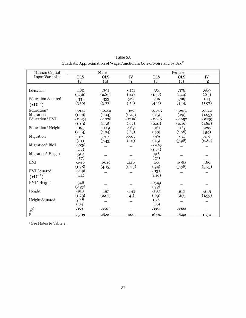
31

Table 6A

Quadratic Approximation of Wage Function in Cote d’Ivoire and by Sexa

Male Female Human Capital Input Variables OLS

(1) OLS (2)

IV (3)

OLS (1)

OLS (2)

IV (3)

Education .480

(3.36) .391

(2.85) -.271 (.41)

.354 (1.30)

.376 (1.44)

.689 (.85)

Education Squared 2( 10 )x −

.331 (3.19)

.333 (3.22)

.362 (.74)

.706 (4.11)

.709 (4.14)

1.14 (1.97)

Education* Migration

-.0147 (1.06)

-.0142 (1.04)

.139 (2.45)

-.0045 (.25)

-.0051 (.29)

.0722 (1.95)

Education* BMI -.0034 (1.83)

-.0028 (1.58)

-.0108 (.92)

-.0046 (2.21)

-.0050 (2.46)

-.0139 (1.82)

Education* Height -.193 (2.44)

-.149 (1.94)

.269 (.69)

-.161 (.99)

-.169 (1.08)

-.297 (.59)

Migration -.179 (.11)

.757 (7.43)

.0017 (.01)

.989 (.45)

.911 (7.98)

.656 (2.82)

Migration* BMI .0036 (.17)

_ _ -.0319 (1.83)

_ _

Migration* Height .512 (.57)

_ _ .418 (.31)

_ _

BMI -.540 (1.98)

.0626 (4.15)

.220 (2.23)

.254 (.94)

.0783 (7.38)

.186 (3.75)

BMI Squared 2( 10 )x −

.0248 (.12)

_ _ -.132 (1.10)

_ _

BMI* Height .348 (2.37)

_ _ .0549 (.33)

_ _

Height -18.3 (1.23)

1.57 (2.67)

-1.43 (41)

-2.37 (.09)

.512 (.67)

-5.15 (1.59)

Height Squared 3.48 (.84)

_ _ 1.26 (.16)

_ _

2R .3531 .3505 _ .3351 .3322 _

F 25.09 28.90 12.0 16.04 18.42 11.70 a See Notes to Table 2.

32

Table 6B

Quadratic Approximations of Wage Function in Ghana and by Sexa

Male Female Human Capital Input

Variables OLS (1)

OLS (2)

IV (3)

OLS (1)

OLS (2)

IV (3)

Education -.0408 (.43)

-.0397 (.39)

.561 (.79)

.198 (1.70)

.195 (1.73)

.600 (.84)

Education Squared 2( 10 )x −

.478 (7.33)

.476 (7.33)

.545 (1.60)

.487 (5.14)

.482 (5.09)

1.05 (2.62)

Education* Migration

-.0205 (2.62)

-.0205 (2.65)

.0118 (.53)

.0181 (1.87)

.0200 (2.10)

.0114 (.53)

Education* BMI -.000 (.04)

.000 (.22)

.0084 (1.14)

-.0034 (3.27)

-.0030 (3.02)

-.0219 (3.85)

Education* Height .0100 (.19)

.0035 (.07)

-.463 (1.13)

-.0968 (1.33)

-.0990 (1.41)

-.122 (.27)

Migration -.582 (.54)

.503 (6.76)

.177 (.88)

.0742 (.00)

.447 (6.01)

.187 (1.18)

Migration* BMI -.0014 (.09)

_ _ .0245 (2.18)

_ _

Migration* Height .660 (1.06)

_ _ -.0643 (.08)

_ _

BMI .197 (.98)

.0479 (3.47)

-.0043 (.05)

-2.06 (1.40)

.0551 (7.70)

.217 (5.59)

BMI Squared 2( 10 )x −

.0956 (.59)

_ _ -.0482 (62)

_ _

BMI* Height -.111 (.98)

_ _ .176 (1.96)

_ _

Height 2.73 (.27)

1.48 (3.21)

8.20 (2.59)

14.9 (1.20)

1.73 (3.73)

8.29 (2.60)

Height Squared 1.85 (.62)

_ _ -5.40 (1.40)

_ _

2R .1871 .1864 _ .1886 .1858 _

F 19.91 22.74 15.20 20.03 22.58 18.65

a

See notes to Table 2.

33

Table 7

Wage Function Estimates for Men and Women Combined with Human Capital Returns Restricted to be Equal and Allowed to Vary by Gender

Côte d’Ivoire (2872) Ghana (6814) Explanatory

Variables OLS (1)

OLS (2)

OLS (3)

OLS (4)

OLS (1)

OLS (2)

OLS (3)

OLS (4)

Male .589 (11.2)

.209 (4.02)

.244 (3.81)

1.30 (.85)

.271 (8.97)

.115 (3.64)

.0512 (1.27)

-.806 (.94)

Education .118 (21.0)

.0937 (16.6)

.0730 (7.71)

.0489 (14.3)

.0395 (11.7)

.0375 (7.71)

Migration .767 (11.7)

.891 (8.87)

.448 (11.1)

.531 (8.98)

BMI .0582 (8.88)

.0613 (7.38)

.0458 (10.5)

.0420 (8.10)

Height .706 (1.90)

.416 (.66)

1.36 (5.89)

1.29 (3.85)

Education *Male

.0357 (3.03)

.0062 (.91)

Migration *Male

-.176 (1.33)

-.183 (2.27)

BMI *Male -.0162 (1.21)

.0110 (1.12)

Height *Male

.446 (.58)

.181 (.39)

34

Table A-1

Means and Standard Deviations for Variables for Earners Age 20 to 60 in

Côte d’Ivoire and Ghana by Sexa

Côte d’Ivoire Ghana Male Female Male Female

A. Dependent Variables Log Hourly Wage Rate 5.77

(1.38) 5.19

(1.53) 3.40 (1.21)

3.17 (1.38)

Years of Education Completed 5.57 (5.45)

2.72 (4.46)

7.13 (5.47)

4.28 (5.06)

Migration (moved from birthplace region at

time of Survey – 1)b

.652 (.476)

.529 (.499)

.333 (.471)

.282 (.450)

Body of Mass Index (Kg./Meters2

) 22.7 (2.95)

24.0 (4.41)

20.9 (2.52)

22.3 (4.22)

Height in Meters 1.70 (.0671)

1.59 (.0576)

1.69 (.0661)

1.58 (.0622)

B. Individual Explanatory Variable: Age 38.2

(10.4) 36.5

(10.3) 36.5

(10.9) 36.3

(11.4)

Rural Residentb

.276 .292 .413 .360

Ethnic Group (CI/G)b

Akan

.223 .257 .432 .480

Krou/Ewe .104 .069 .172 .172 Mande South/Gaadangbe .081 .123 .086 .096 Mande North/Dagbani .083 .087 .039 .025 Voltaic/Hausa .061 .060 .020 .023 Other/Other .170 .114 .238 .193 ---/Nzema -- -- .012 .011 Birthplace Region (11) (11) (11) (11)

Religionc

-- -- .012 .011

C. Parent Characteristics: Mother’s Years of Education .0714

(.633) .144

(.1.06) .627

(2.36) .811

(2.80) Father’s Years of Education .667

(2.24) .825

(2.71) 2.31

(4.61) 2.67

(4.95)

Father’s Education Unknownb

.011 .015 .008 .011

Years Mother Worked in Agriculture .513 .581 .656 .626 Years Father Worked in Agriculture .764 .772 .712 .679 D. Sample Cluster or Community Characteristic:

Health Problems (first or second)b

Malaria

.036 .045 .423 .403

Diarrhea .051 .069 .154 .156 Measles .050 .043 .268 .267

Water/Sanitation Problemsb

.030 .033 .169 .155

Distance to Hospital or Clinic (km/miles) 2.97 (7.42)

2.34 (6.67)

4.17 (7.08)

3.56 (6.10)

Distance to Nurse or Doctor (km/miles) 3.58

(9.38) 2.83

(7.77) 3.53

(6.75) 2.99

(5.89)

Prices of Food Items and Staplesd

(8) (8) (11) (11)

35

Rainfall Annual (mm) 112. (18.1)

111. (18.3)

49.7 (14.5)

49.2 (14.5)

Interview Occurred in Rainy Seasonb

North

.111 .108 .077 .056

South .525 .527 .557 .548

Immunization Campaign (in last years = 1)b

f f .469 .473

Anti Malaria Campaign (in last 5 years)b

f f .284 .274

Preventive Public Health Expenditures per

capitae

f f 93.0 (20.3)

92.1 (20.3)

Community Characteristics (cont.)

Curative Public Health Expenditures per capitae

n/a n/a 226. (77.7)

228. (78.7)

Distance to Market (km/miles) .761 (2.63)

.814 (3.11)

3.06 (6.55)

2.94 (6.14)

Distance to Primary School (km/miles) .0904 (.635)

.0398 (.343)

.307 (1.11)

.256 (.962)

Distance to Middle School (km/miles) f f 1.25 (2.61)

1.01 (2.35)

Distance to Secondary School (km/miles) 7.94

(16.6) 7.53

(14.8) 8.39

(12.7) 7.21

(11.5)

Notes: a

Sample was restricted to individuals reporting the following: 1.4 < Height < 2.0; 35 < weight < 115; 12 < BMI <45; and 19< Age < 61. Except for age the anthropometric restrictions eliminated 1 to 7 persons each.

b Dummy variable. Standard variation of variable is equal to (1 )m m− , where m denotes the mean of

binary variable. c

Christian, Muslim, Traditional, and other. d

In Côte d’Ivoire prices refer to Beef, Fish, Rice, Onion, Peanut Butter, Palm Oil, Manioc, and Banana. In Ghana prices refer to Cassova, Maize, Banana, Onion, Tomato, Eggs, Fish, Palm Oil, Peanuts, Sugar and Antibiotic.

e Available from Government Budget allocations by regions only for Ghana in 1987.

f Not appropriate to Côte d’Ivoire educational system or no questions asked.

36

Table A-2

Correlations Between Wage and Human Capital Variables:

Côte d’Ivoire and Ghana by Sexa

Female: Côte d’Ivoire (1)

Log Wage (2)

Education (3)

Migration (4)

BMI (5)

Height Male: 1. Log Hourly Wage _ .346

(.0001) .211

(.0001) .271

(.0001) .110

(.0002) 2. Education Years .484

(.0001) _ .051

(.081) .116

(.0001) .177

(.0001) 3. Migration .253

(.0001) .171

(.0001) - .097

(.0008) .101

(.0005) 4. Body Mass Index .228

(.0001) .159

(.0001) .101

(.0001) _ .039

(.180) 5. Height Meters .112

(.0001) .131

(.0001) .097

(.0001) .028

(.255) _

Ghana Female: Male: 1. Log Hourly Wage _ .219

(.0001) .109

(.0001) .207

(.0001) .088

(.0001) 2. Education Years .232

(.0001) _ .078

(.0001) .147

(.0001) .126

(.0001) 3. Migration .135

(.0001) .074

(.0001) _ .139

(.0001) .044

(.0101) 4. Body Mass Index .161

(.0001) .172

(.0001) .076

(.0001) - .048

(.0049) 5. Height Meters .097

(.0001) .056

(.0010) .042

(.0148) .048

(.0046) _

a

Sample of all persons age 20 to 60 reporting information needed to construct hourly wage rate. Sample size is 1692 for men and 1180 for women in Côte d’Ivoire and 3414 for men and 3400 for women in Ghana. Beneath the reported zero order correlation is the p value at which the correlation is statistically significant.

37

Table A-3

Size of Côte d’Ivoire Panel Sample when Restrictions are Imposed to Determine a “Matched” Individual Record

Sample Restrictions Males Females

All Persons Age Initially between 20-60 with Identical Household and Individual Number

809 498

Same Sex in Two Periods 768 462

Age Within 10 Years, i.e., [Age 1 + 1 -

Age 2 ]≤ 10

742 427

Age Within 10 Years, i.e., [Age 1 + 1 -

Age 2 ]≤ 5

712 409

Age Within 2 Years 662 357

Working Sample: Age Within 5 Years and Education Within 5 Years

685 397

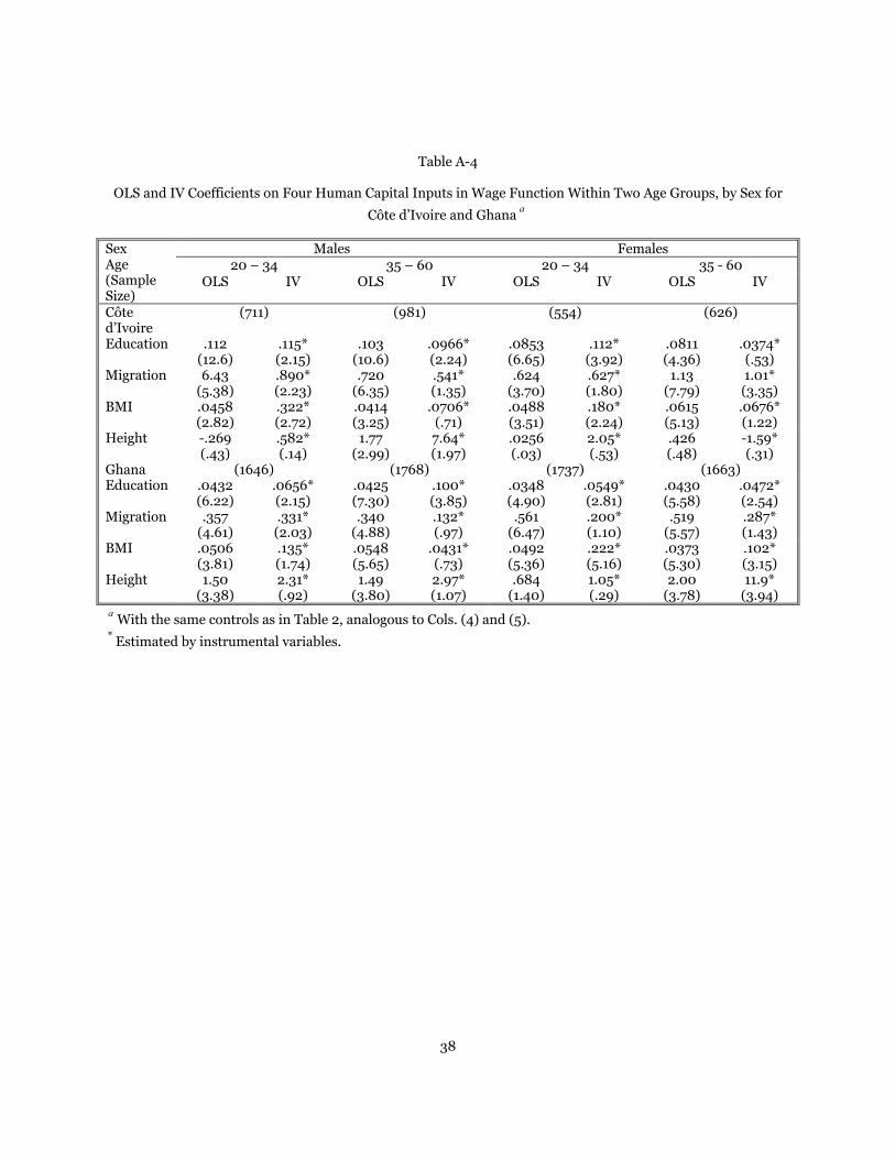
38

Table A-4

OLS and IV Coefficients on Four Human Capital Inputs in Wage Function Within Two Age Groups, by Sex for

Côte d’Ivoire and Ghanaa

Males Females 20 – 34 35 – 60 20 – 34 35 - 60

Sex Age (Sample Size)

OLS IV OLS IV OLS IV OLS IV

Côte d’Ivoire

(711) (981) (554) (626)

Education .112 (12.6)

.115* (2.15)

.103 (10.6)

.0966* (2.24)

.0853 (6.65)

.112* (3.92)

.0811 (4.36)

.0374* (.53)

Migration 6.43 (5.38)

.890* (2.23)

.720 (6.35)

.541* (1.35)

.624 (3.70)

.627* (1.80)

1.13 (7.79)

1.01* (3.35)

BMI .0458 (2.82)

.322* (2.72)

.0414 (3.25)

.0706* (.71)

.0488 (3.51)

.180* (2.24)

.0615 (5.13)

.0676* (1.22)

Height -.269 (.43)

.582* (.14)

1.77 (2.99)

7.64* (1.97)

.0256 (.03)

2.05* (.53)

.426 (.48)

-1.59* (.31)

Ghana (1646) (1768) (1737) (1663) Education .0432

(6.22) .0656* (2.15)

.0425 (7.30)

.100* (3.85)

.0348 (4.90)

.0549* (2.81)

.0430 (5.58)

.0472* (2.54)

Migration .357 (4.61)

.331* (2.03)

.340 (4.88)

.132* (.97)

.561 (6.47)

.200* (1.10)

.519 (5.57)

.287* (1.43)

BMI .0506 (3.81)

.135* (1.74)

.0548 (5.65)

.0431* (.73)

.0492 (5.36)

.222* (5.16)

.0373 (5.30)

.102* (3.15)

Height 1.50 (3.38)

2.31* (.92)

1.49 (3.80)

2.97* (1.07)

.684 (1.40)

1.05* (.29)

2.00 (3.78)

11.9* (3.94)

aWith the same controls as in Table 2, analogous to Cols. (4) and (5).

*Estimated by instrumental variables.

39

Table A-5a

Human Capital Demand Equations Used to Instrument Inputs in Wage Function in Côte d’Ivoire:

Selected Variablesa

Male Female Country, Sex Explanatory

Variableb

Education Migration BMI Height Education Migration BMI Height

Mother’s Education .165 (.90)

0070 (.50)

.114 (.95)

.0003 (.14)

.371 (3.42)

-.0099 (1.02)

-.212 (1.55)

.0051 (2.86)

Father’s Education .257 (4.43)

.0033 (.75)

.0325 (.85)

.0013 (1.54)

.387 (8.19)

.0006 (.15)

.0439 (.74)

-.0010 (1.35)

Father’s Education Unknown

3.75 (3.53)

.120 (1.48)

1.82 (2.61)

.0300 (1.90)

1.70 (2.00)

-.0963 (1.27)

.104 (.10)

-.0329 (2.37)

Mother Employed in Agriculture

-1.50 (6.22)

-1.53 (8.32)

-.310 (1.96)

-.0082 (2.29)

-.998 (4.05)

-.167 (7.56)

-.93 (3.00)

-.0040 (.99)

Father Employed in Agriculture

-.219 (.70)

.0235 (.98)

.266 (1.29)

-.0077 (1.66)

-1.29 (4.19)

.0179 (.65)

-2.13 (.55)

-.0049 (.98)

Rural Residentc

.654 (1.3)

.752 (20.9)

.326 (1.05)

-.0047 (.67)

-.471 (1.14)

.798 (21.7)

-.142 (.27)

-.0042 (.62)

Rainfallc

.0740 (2.92)

-.0069 (3.55)

.0068 (.41)

.0009 (2.33)

.0032 (.21)

-.0114 (8.31)

.0105 (.54)

-.0002 (.86)

Health Problems: Malaria

1.01 (1.92)

-.0238 (.36)

-1.12 (1.96)

.0120 (.93)

-.327 (49)

-.170 (2.87)

-.388 (.47)

-.0088 (.81)

Diarrhea -1.47 (1.92)

-.130 (2.22)

.181 (.36)

-.0149 (1.31)

-.0800 (.13)

-.111 (2.08)

-1.21 (1.61)

-.0044 (.45)

Measles -.823 (.85)

.0721 (.97)

.127 (.20)

.0074 (.52)

-1.36 (1.51)

-.330 (4.10)

-1.17 (1.04)

-.0265 (1.79)

Sanitation and Water

-.608 (.59)

-.287 (3.61)

.448 (.66)

.0105 (.68)

-1.28 (1.50)

-.277 (3.65)

-2.74 (2.56)

-.0090 (.64)

Distance to Clinic or Hospital

-.0265 (.67)

.0108 (3.59)

-.0426 (1.64)

-.0003 (.52)

.0169 (.33)

.0408 (8.99)

.0687 (1.08)

.0003 (.40)

Distance to Nurse or Doctor

.0162 (.52)

-.0102 (4.29)

.0400 (1.96)

.0002 (.44)

.0020 (.05)

-.0199 (5.51)

-.0723 (1.42)

.0004 (.61)

Distance to Permanent Market

-.0541 (.95)

-.0118 (2.69)

-.0200 (.53)

-.0016 (1.88)

-.0370 (.83)

-.0252 (6.34)

-.0812 (1.45)

-.0012 (1.62)

Distance to Primary School

.0808 (.42)

-.0074 (.50)

-.0741 (.58)

.0062 (2.18)

.188 (.61)

.144 (5.20)

.438 (1.13)

-.0067 (1.31)

Distance to Secondary School

.0187 (1.03)

-.0031 (2.23)

-.0174 (1.45)

.0002 (.86)

.0166 (1.02)

.0043 (2.94)

.0116 (.57)

.00058 (2.18)

a

Beneath regression coefficient in parentheses is absolute value of t. b

Other control variables include 4 age dummies, 6 ethnic groups, 10 regions, 10 local food prices, and 5 rainy season malaria interactions.

cThese variables are also in the wage function, and thus do not represent identifying instrumental variables, i.e., they are in Y and not in X.

40

Table A-5b

Human Capital Demand Equations Used to Instrument Inputs in Wage Function in Côte d’Ivoire:

Selected Variablesa

Male Female Country, Sex Explanatory

Variableb

Education

Migration BMI Height Education

Migration BMI Height

Mother’s Education

.0779 (2.13)

-.0007 (.27)

-.0300 (1.45)

.0006 (1.03)

.226 (8.16)

-.0014 (.70)

-.0528 (1.88)

.0000 (.13)

Father’s Education .122 (5.63)

.0025 (1.72)

.0425 (3.67)

.0000 (.15)

.209 (11.4)

.0014 (1.07)

-.0148 (.80)

.0003 (1.16)

Father’s Education Unknown

.687 (.81)

-.0147 (.26)

-.684 (1.41)

.0215 (1.66)

-.116 (1.75)

-.0339 (.72)

.742 (1.10)

.0029 (.28)

Mother Employed in Agriculture

-.725 (3.97)

-.0774 (6.24)

-.605 (5.81)

-.0126 (4.54)

-.904 (5.34)

-.101 (8.42)

-1.51 (8.80)

-.0031 (1.16)

Father Employed in Agriculture

-.424 (2.03)

-.0014 (.10)

.108 (.91)

-.0019 (.60)

-.605 (3.21)

-.0066 (.49)

-.412 (2.16)

-.0058 (1.97)

Rural Residentc

.101 (.46)

.921 (61.4)

.165 (1.32)

.0069 (2.09)

-.0333 (.16)

.889 (62.3)

.629 (3.08)

.0067 (2.12)

Rainfallc

.0063 (.46)

-.0059 (6.32)

.0153 (1.96)

-.0003 (1.68)

.0102 (.86)

-.0047 (5.65)

-.0113 (.94)

-.0003 (1.62)

Health Problems: Malaria

-.769 2.47)

-.0647 (3.06)

-.339 (1.92)

-.0143 (3.03)

.299 (1.08)

-.0237 (1.21)

-.275 (.98)

.0017 (.40)

Diarrhea -.204 (.78)

-.136 (7.62)

.117 (.79)

-.0000 (.01)

-.0752 (.32)

-.160 (9.60)

-.601 (2.51)

.0051 (1.38)

Measles .506 (1.70)

-.141 (6.96)

-.239 (1.41)

.0065 (1.43)

-.111 (.40)

-.0995 (5.15)

-.0975 (.35)

.0043 (.99)

Sanitation and Water

.274 (1.00)

.142 (7.62)

.0397 (.26)

-.0031 (.76)

.276 (1.09)

.187 (10.4)

-.139 (.52)

-.0062 (1.56)

Immunization Campaign in 5 years

-.231 (.64)

-.0922 (3.74)

-.180 (.88)

-.0019 (.35)

-.994 (3.03)

-.104 (4.50)

-.533 (1.60)

-.0037 (.72)

Distance to Nurse or Doctor

.0282 (1.22)

-.0021 (1.37)

.0131 (1.00)

.0005 (1.32)

.0279 (1.25)

-.0002 (.13)

.0179 (.79)

.0000 (.16)

Distance to Permanent Market

.0069 (.38)

-.0106 (8.65)

-.0031 (.37)

.0005 (1.32)

.0279 (1.25)

-.0002 (.13)

-.0223 (1.36)

.0002 (.67)

Distance to Primary School

-.198 (1.69)

-.503 (6.32)

-.0778 (1.17)

-.0042 (2.27)

-.0539 (.45)

-.0253 (2.99)

-.196 (1.61)

-.0011 (.56)

Distance to Middle School

-.199 (3.85)

-.0373 (10.6)

-.0399 (1.36)

.0007 (.87)

-.124 (2.31)

-.0368 (9.69)

-.0820 (1.51)

.0012 (1.38)

Distance to Secondary School

-.0283 (2.49)

-.0076 (9.86)

-.0011 (.16)

.0005 (2.66)

-.0189 (1.68)

-.0073 (9.26)

-.0223 (1.96)

-.0002 (1.34)

a

Beneath regression coefficient in parentheses is absolute value of t. b

Other control variables include 4 age dummies, 6 ethnic groups, 10 regions, 10 local food prices, 5 rainy season malaria interactions, state level per capita public expenditures on preventive and curative health programs in 1987 and anti malaria campaign in last five years.

cThese variables are also in the wage function and thus do not represent identifying instrumental variables, i.e., they are in Y and not in X.

41

APPENDIX FIRST-STAGE HUMAN CAPITAL INPUT ESTIMATES

The coefficients on some of the identifying instrumental variables (X) in the linear human capital input demand

equations are reported in Tables A-5a and A-5b for Cote d’Ivoire (the Ivory Coast) and Ghana. A few regularities might be

noted. Parent educations are particularly important in determining the child's education. The father's education has a

somewhat larger coefficient than the mother's in the son's education equation, but in the daughter's education equation they

have about the same magnitude (C.F. Thomas, 1994). Having a mother employed in agriculture has a uniformly negative

and substantial effect on all four human capital inputs for males and females in both countries. Residing a greater distance

from a permanent market, and with various local health problems, reduces the chances of out migration. The effects of

distance to primary and secondary schools reduce educational attainment in Ghana, as it also is negatively correlated with

migration and often height and weight. It should be noted that rural residence and rainfall, which are strongly related to out

migration, are not identifying variables, because they also enter the wage function directly.

Given the high degree of intercorrelation between the local sample cluster characteristics, individual variables

may exhibit erratic relationships with the input demands due to multicollinearity, e.g., the distance to doctors and hospitals

are correlated at about.8 (Schultz and Tansel, 1997). It should also be recognized that because all of the instruments, with

the exception of the parent characteristics, they are measured at the level of the sample cluster, of which there are only

about one hundred, the standard errors on these and other variables may be slightly downward biased. Deaton (1997) has

stressed the need to adjust the standard errors when such "aggregated" variables are used to condition a relationship. The

larger sample of individuals overstates the true sample size in the calculation of significance levels for the community

variables. In the IV estimates reported in the paper, the instruments in Table A-5 are also interacted with rural residence,

rainfall and quadratics in mother's and father's education added to the interacted instrument list as discussed in the text.

42

Endnotes

1 Another human resource program that should be analyzed as an argument in the wage function is family

planning. Family planning performs several functions, one of which helps women avoid unwanted births by reducing the

cost of effective birth control. Unwanted births may be associated with women sacrificing their career objectives, if that

career is imperfectly compatible with childbearing. In studies of Malaysia and the United States, an unanticipated or

unwanted birth is associated with women receiving a wage in the labor market that is 10 percent lower (Schultz, 1992:

Table 5.1).

2 Social externalities associated with human capital are not accounted for in this study but might be addressed with

micro data with a sufficiently structured model describing the source and scope of the diffusion of the externality. For

example, Foster and Rosenzweig (1995) consider the effects on a farmer's profits of learning from a neighbor's innovative

adoption of new productive inputs in India. Health may also increase the capacity to work in addition to its effect on wage

rates that is estimated here. Schultz and Tansel (1997) discuss and estimate wage and labor supply effects of adult illness.

3 There are several hypotheses for why the inputs might be correlated which stem from heterogeneity and

technology: (1) exogenous family wealth relaxes the budget constraint allowing more wealthy families to invest more in

all forms of human capital in their children, driving down the marginal returns to these investments due to the family's

lower than average opportunity cost of capital; (2) an individual's biological endowment may raise the returns to several

forms of human capital, as for example, it is hypothesized that ability increases the returns to education (Becker, 1993;

Griliches, 1977); (3) heterogeneity in preference of families could also lead to differences across individuals in amounts of

all human capital investments; and finally (4) types of human capital may technically complement (or substitute) for each

other in the wage function, leading individuals who maximize their joint returns on all human capital investments to

concentrate on complementary inputs and specialize between substitute inputs.

4 The first three hypotheses for an intercorrelation in human capital inputs conditional on household and regional

variables that were listed in endnote 3 could also be used to justify the treatment of these inputs as endogenous to the wage

function. They operate across inputs as an unobserved constraint on the household—unobserved wealth, individual

endowments, and preferences—and could therefore equally well-affect wages through other unspecified channels as well

as through their effect on the demand for observed forms of human capital.

43

5 The same framework could be extended to education, where some portion of the variation in education is

determined by the genetic distribution of ability and the remainder is potentially reproducible.

6 Unobserved heterogeneity in individuals may also explain why those who invest more in any particular form of

human capital may earn lower (or higher) returns at the margin. As noted above, these sources of heterogeneity bias in

input demands would be corrected when the inputs are treated as endogenous to the wage function.

7 For example, it has been noted that children who are taller for their age (or of greater weight for age) perform

better in school (Moock and Leslie, 1986). More educated individuals are more likely to migrate, even when controlling

for wage and unemployment rates at origin and destination (Schultz, 1982). If either migration or education is determined

endogenously, then a positive effect of the human capital interaction variable based on the assumption they are exogenous

in the wage function may not be a valid indication of their technological interactions (Vijverberg, 1993). Similar doubts

attach to the hypothesis that longevity should enhance the returns to, and hence demands for, educational human capital

(Ram and Schultz, 1979).

8 This production function retains the logarithmic transformation of the dependent variable, the wage rate, because

the residuals from wage equations estimated in logarithms are more nearly normally distributed than are the residuals to a

wage function estimated in absolute levels. Box-Cox transformation analyses of wage data often indicate that the log

transformation does not perfectly fit wages, but tends to be a better approximation than the linear specification. The

translog function is another commonly used second-order approximation, in which all inputs may only take on positive

values, which education and migration generally violate (Fuss and McFadden, 1978). The translog specification was not

superior to the Leontief-Diewert estimates reported here, with the minimum value of education assumed to be one year.

Interactions between age and the human capital inputs probably also need to be re-appraised (Angrist and Newey, 1991),

which could reflect the different productive value of each human capital input at different biological ages, or it could

reflect the different quality of that input produced at different times embodied in different birth cohorts.

9 There are several reasons one might expect human capital inputs to be correlated across individuals in equation

(1), due to observable variables, unobservable variables, preferences, and technology. Unfortunately, in the form of the

model estimated here it is not possible to distinguish among these possible causes: (a) Lifetime full wealth constraints

44

could induce demand for various human capital inputs in a child, to the extent that these inputs enter the parent's utility as

a normal altruistic consumption good. (b) Wealth might also reduce the cost of parent borrowing, relax credit constraints,

and thereby encourage the derived demand of wealthier parents for the services of child human capital. Evidence that

economic shocks to parents lead to responses in child health and schooling investments do not, therefore, satisfactorily

distinguish between the role of credit constraints on parents and the value of child human capital as a parental consumption

good (Foster, 1995; Jacoby, 1993). (c) Characteristics of the individual, such as ability, that are omitted from the wage

function may affect the returns to several forms of human capital, such as schooling and migration (Schultz, 1982). (d)

Parents or society may respond to heterogeneity as in (c) by compensating or reinforcing behavior, depending on their

relative preferences for equality and efficiency (Becker, 1993). (e) Differences in parent preferences for child human

capital could explain why some parents invest relatively more in all forms, and some parents invest in less. (f) The

technology of human capital production and its utilization in the labor market may cause different forms of child human

capital to be complements or substitutes from the family's perspective, enhancing or depressing the returns to other forms.

10 These wealth variables are theoretically expected to increase the individual's labor productivity in non-wage

employment and increase demand for leisure, both of which tendencies would raise the market reservation wage and

reduce the likelihood of participating as a wage earner. Estimation of the probit for being an earner that includes all of the

variables in the wage function plus the physical wealth identifying variables indicated that these physical wealth variables

are significantly associated with a reduction in wage earning participation in these samples.

11 For the Ivory Coast, the three years 1985-87 are combined for a total sample of about 40,000 persons. For wage

earners and self-employed who reported labor earnings and hours worked in that activity, a wage rate is derived. This

group of earners between the ages of 15 and 65 is comprised of 1602 men out of 5642 and 768 women out of 6579.

Ainsworth and Muñoz (1986) describe the design of these surveys. For Ghana, two years of surveys are combined from

1987-88 and 1988-89 with a sample of about 30,000 persons. The wage-earner sample yielded 3521 men out of 5034

between the ages of 15 and 65, and 3408 females out of 5834. The anthropometric variables (i.e., height and BMI) were

not collected for all individuals, which also restricted the size of these working samples slightly. The later analysis of labor

earnings is restricted to men and women age 20 to 60 reporting positive labor earnings and hours last month or last year.

The means and standard deviations on all variables for these working samples are reported in appendix Table A-1.

45

12 The summary measure of years of education completed does not weight the much larger private opportunity cost

of a year of secondary or tertiary schooling compared with primary schooling, or the likelihood that the "quality" of a year

of schooling has changed over time. Nor does this measure of stocks of education capture adequately past national

investments, because international migration is selective for education. Better-educated Ghanaians emigrated in large

numbers during the 1970s and 1980s, whereas the growing economy of Ivory Coast attracted immigrants from lower-

income neighboring countries (Schultz and Tansel, 1997).

13 And similar to that reported for Japan among men reaching age 20 for the 45 years 1892 to 1937 of .88 cm./decade

(Shay, 1994).

14 An empirical criterion for identification as originally proposed by Basmann (1960) relies on testing the explanatory

power of adding X to the wage equation (2). A significant correlation between X and v calls into question the validity of X

instrument for estimating 1 in the wage equation.

15 Surprisingly, the instrumental variable auxiliary equation for higher yields to a larger coefficient of determination

for older than younger persons in both the Ivory Coast and Ghana (C.F. Table A-4)

16 This does not appear to be a serious source of bias in the case studied here because the five parent characteristics are

not strongly related to the wage of their child, although they are often related to the child’s human capital inputs. When

the five parent variables are added to the OLS estimates of the wage function (Table 2, Col 4), they are never statistically

significant at the 5 percent level, i.e., the F ratios with five and n-32 degrees of freedom are less than the critical value of

2.3 in the four contry/sex samples.

17 In these African samples relatively few individuals are siffuciently obese that BMI would decrease health, with only 1-

2 percent of the men reporting BMI in excess of 28 and 6-10 percent of the women. Efforts to estimate non-linearities in

the wage equation with all of the other controls (Table 6). See Strauss and Thomas (1995) for other evidence of the non-

linear patterns between nutritional inputs and wage rates and income.

18 The joint F test of the statistical significance of the identifying instrumental variables provides an indication of the

46

power or reliability of the IV estimates. See discussion of Bound et al., 1995.

19 Note however, that education and migration and their interaction are not treated as part of the information set to

condition the predictions of the endogenous inputs and their interactions.

20 Another investigation of the Ghana survey found that the instrumental variable estimate of the effect of height, BMI,

and schooling on child cognitive ability found the schooling IV and OLS estimates were similar, but the IV estimates for

height and BMI increased 4-6 fold (Behrman and Lavy, 1995). This outcome may also be explained by the distinction

drawn in this paper between the differential effect of reproducible and innate anthropometric variation as well as the

measurement error embodied in these human capital inputs.

21 An alternative counterfactual would concentrate on particular changes in (exogenous) policy variables, and reckon their

effects on human capital accumulation and wage changes. But these estimates of the human capital input demand

equations are not offered as structural equations pivoting on well measured variation in policy regime for which future

changes might be forecast, but a reduced form equations for human capital demands with many exogenous but highly

correlated conditioning variables for which any single or group of estimated effects could be misleading. Another

approach is to consider how some of the key conditioning variables have changed between the older and younger

generation, or in the case of education between the parent and child’s generations. If the equation continued to predict

outcomes in the next generation, we would then have some basis for projecting change in the human capital inputs and

being able to translate these input changes into predicted wage changes.

22 The panel structure to the survey in Ghana could not be recovered because the household and individual identification

numbers were not replicated.

23 To assess the accuracy of observations of BMI the changes in BMI were plotted against the number of days in the last

month the individual was ill and unable to work, separately for the first and the second year of each panel. The

correlations were not statistical significant, although these patterns suggested that those who were sick more days in the

second year were more likely to have reduced their BMI between the years, as expected.

47

24 The effect of measurement error on estimates of models based on panel data is explored by Griliches and Hausman

(1986), in which serial correlation in botht he outcome variable and in the measurement error are discussed. Because the

input variables are not sugject to valid or substantial variation, with the possible exception of BMI, it is not possible here

to estimate the wage function from first differences. Also, to require that the individual report wages in both survey cycles

reduces further the small working sample examined here.

25 The re-interviewer is instructed to return to the same household and confirm that the occupants are the same, by

identifying the same head of household or their spouse. A new household member is assigned to the occupants if neither

the head of household or the spouse is the same. Individuals in the matched household are then matched to the individual

names and unique identification numbers from the first round household roster. Given the larger size and more complex

kinship structures of households in the Ivory Coast and Ghana than in most high-income countries, it would not be

surprising if mismatches are more common in these two low-income countries. The economic incentives for the survey

interviewers are also likely to favor reported matches to save their time, even when there is reasonable doubt about the

validity of the match.

26 The household survey interviewers have little incentive to report the residents at a specific sample address as changed

from the previous year, for this will necessitate their interviewing a new “replacement” household. Similarly, if

individuals in a household change between annual interviews, it is possible that a new person in a household will be coded

to match that of an individual enumerated before but absent at the time of the second interview.

27 Without any restrictions on the consistency of reporting of age and education in the two panel observations leads to a

lower serial correlation of education of .95 and lower correlations for the other matched human capital inputs as well.

28 The variance in measured women’s height is estimated as .0035 in Table 4, whereas the correlation between height in

adjacent years if .788, indicating that the variance in measurement error is about .0008 = (1-.788)*.0035, or roughly one-

fourth the magnitude of the variance of the signal of .0027. In the case of female education, the variance of the signal is

estimated from Table 4 as 25.6, and the variance in the measurement error of female education is .42, suggesting a signal

to error ration of about 60.

48

29 One possible cause of heterogeneity is the omitted variable of pregnancy, a condition which may affect negatively

labor productivity and affect positively BMI, and thus reduce OLS estimates of the positive effect of BMI on the wage of

women. However, because fertility is to some degree a choice variable, the probability of becoming pregnant need not be

independent of human capital demands. Consequently, conditioning the wage function on pregnancy status could itself

bias other estimates, for example, biasing downward the wage return to a woman’s education. Lacking a suitable

instrument that might identify the fertility decision rule as distinct form other human capital investments (X) or wage

determinants (Y), it is not obvious how the casual relationship between pregnancy and productivity can be empirically

assessed here. This source of heterogeneity bias could help to explain why IV panel estimates of BMI in Table 5 are more

than twice as large as OLS estimates for women, but only half again larger for men.

30 Height and BMI variable were also fit in logarithms but did not improve standard fit measures, in either the linear or

quadratic forms (C.F. Strauss and Thomas, 1995).

31 The true human capital inputs should be nearly perfectly correlated in adjacent years, because height and migration

cannot validly change, and education and BMI should vary little. Instead the serial correlation of education is .98 while

that for BMI and height varies from .79 to .91 confirming again the greater importance measurement error in height and

BMI than in education.