Embed Size (px)
Citation preview


W. Greiner · S. Schramm · E. SteinQUANTUM CHROMODYNAMICS

GreinerQuantum MechanicsAn Introduction 4th Edition
GreinerQuantum MechanicsSpecial Chapters
Greiner · MüllerQuantum MechanicsSymmetries 2nd Edition
GreinerRelativistic Quantum MechanicsWave Equations 3rd Edition
Greiner · ReinhardtField Quantization
Greiner · ReinhardtQuantum Electrodynamics3rd Edition
Greiner · Schramm · SteinQuantum Chromodynamics3nd Edition
Greiner · MaruhnNuclear Models
Greiner · MüllerGauge Theory of Weak Interactions3rd Edition
GreinerClassical MechanicsSystems of Particlesand Hamiltonian Dynamics
GreinerClassical MechanicsPoint Particles and Relativity
GreinerClassical Electrodynamics
Greiner · Neise · StöckerThermodynamicsand Statistical Mechanics

Walter Greiner ·Stefan SchrammEckart Stein
QUANTUMCHROMODYNAMICS
With a Foreword byD.A. Bromley
Third Revised and Enlarged EditionWith 165 Figures,
and 66 Worked Examples and Exercises
123

Prof. Dr. Dr. h. c. mult. Walter GreinerFrankfurt Institute for Advanced Studies (FIAS)Johann Wolfgang Goethe-UniversitätMax-von-Laue-Str. 160438 Frankfurt am MainGermany
email: [email protected]
Prof. Dr. Stefan SchrammCenter for Scientific Computing (CSC)Johann Wolfgang Goethe-UniversitätMax-von-Laue-Str. 160438 Frankfurt am MainGermany
email: [email protected]
Dr. Eckart SteinPhysics DepartmentMaharishi University of Management6063 NP VlodropThe Netherlands
email: [email protected]
Title of the original German edition: Theoretische Physik, Ein Lehr- und Übungsbuch, Band 10:Quantenchromodynamik c©Verlag Harri Deutsch, Thun, 1984, 1989
ISBN-10 3-540-48534-1 Springer Berlin Heidelberg New YorkISBN-13 978- 3-540-48534-6 Springer Berlin Heidelberg New YorkISBN-10 3-540-66610-9 2nd Ed. Springer Berlin Heidelberg New York
Library of Congress Control Number: 2006938282
This work is subject to copyright. All rights are reserved, whether the whole or part of the material is concerned,specifically the rights of translation, reprinting, reuse of illustrations, recitation, broadcasting, reproduction on mi-crofilm or in any other way, and storage in data banks. Duplication of this publication or parts thereof is permittedonly under the provisions of the German Copyright Law of September 9, 1965, in its current version, and permissionfor use must always be obtained from Springer. Violations are liable for prosecution under the German CopyrightLaw.
Springer is a part of Springer Science+Business Media
springer.com
c©Springer-Verlag Berlin Heidelberg 1994, 2002, 2007
The use of general descriptive names, registered names, trademarks, etc. in this publication does not imply, even inthe absence of a specific statement, that such names are exempt from the relevant protective laws and regulationsand therefore free for general use.
Typesetting: LE-TEX Jelonek, Schmidt & Vöckler GbRProduction: LE-TEX Jelonek, Schmidt & Vöckler GbRCover: eStudio Calamar S. L., Spain
SPIN 11864288 56/3100YL - 5 4 3 2 1 0 Printed on acid-free paper

Foreword to Earlier Series Editions
More than a generation of German-speaking students around the world haveworked their way to an understanding and appreciation of the power and beautyof modern theoretical physics – with mathematics, the most fundamental ofsciences – using Walter Greiner’s textbooks as their guide.
The idea of developing a coherent, complete presentation of an entire fieldof science in a series of closely related textbooks is not a new one. Many olderphysicists remember with real pleasure their sense of adventure and discoveryas they worked their ways through the classic series by Sommerfeld, by Planckand by Landau and Lifshitz. From the students’ viewpoint, there are a greatmany obvious advantages to be gained through use of consistent notation, logi-cal ordering of topics and coherence of presentation; beyond this, the completecoverage of the science provides a unique opportunity for the author to conveyhis personal enthusiasm and love for his subject.
The present five volume set, Theoretical Physics, is in fact only that part ofthe complete set of textbooks developed by Greiner and his students that presentsthe quantum theory. I have long urged him to make the remaining volumes onclassical mechanics and dynamics, on electromagnetism, on nuclear and particlephysics, and on special topics available to an English-speaking audience as well,and we can hope for these companion volumes covering all of theoretical physicssome time in the future.
What makes Greiner’s volumes of particular value to the student and profes-sor alike is their completeness. Greiner avoids the all too common “it followsthat . . . ” which conceals several pages of mathematical manipulation and con-founds the student. He does not hesitate to include experimental data to illumi-nate or illustrate a theoretical point and these data, like the theoretical content,have been kept up to date and topical through frequent revision and expansion ofthe lecture notes upon which these volumes are based.
Moreover, Greiner greatly increases the value of his presentation by includ-ing something like one hundred completely worked examples in each volume.Nothing is of greater importance to the student than seeing, in detail, how thetheoretical concepts and tools under study are applied to actual problems of inter-est to a working physicist. And, finally, Greiner adds brief biographical sketchesto each chapter covering the people responsible for the development of the the-oretical ideas and/or the experimental data presented. It was Auguste Comte(1798–1857) in his Positive Philosophy who noted, “To understand a scienceit is necessary to know its history”. This is all too often forgotten in modern

VI Foreword to Earlier Series Editions
physics teaching and the bridges that Greiner builds to the pioneering figures ofour science upon whose work we build are welcome ones.
Greiner’s lectures, which underlie these volumes, are internationally notedfor their clarity, their completeness and for the effort that he has devoted to mak-ing physics an integral whole; his enthusiasm for his science is contagious andshines through almost every page.
These volumes represent only a part of a unique and Herculean effort to makeall of theoretical physics accessible to the interested student. Beyond that, theyare of enormous value to the professional physicist and to all others working withquantum phenomena. Again and again the reader will find that, after dipping intoa particular volume to review a specific topic, he will end up browsing, caughtup by often fascinating new insights and developments with which he had notpreviously been familiar.
Having used a number of Greiner’s volumes in their original German in myteaching and research at Yale, I welcome these new and revised English trans-lations and would recommend them enthusiastically to anyone searching fora coherent overview of physics.
Yale University D. Allan BromleyNew Haven, CT, USA Henry Ford II Professor of Physics1989

Preface to the Third Edition
The theory of strong interactions, quantum chromodynamics (QCD), was for-mulated more than 30 years ago and has been ever since a very active fieldof research. Its continuing importance may be estimated by the Nobel prize inphysics for the year 2004, which was awarded to Gross, Wilczek, and Politzerfor their discovery of asymptotic freedom, one of the key features of QCD. Theunderlying equations of motion for the gauge degrees of freedom provided byQCD are nonlinear and minimally coupled to fermions with global and localSU(3) charges. This leads to spectacular problems compared with those of QEDsince the gauge bosons themselves interact with each other. On the other hand,it is exactly the self-interaction of the gluons which leads to asymptotic freedomand the possibility to calcuate quark–gluon interaction at small distances in theframework of perturbation theory. We discover one of the most complicated butmost beautiful gauge theories which poses extremely challenging problems onmodern theoretical and experimental physics today.
Quantum chromodynamics is the quantum field theory that allows us to cal-culate the propagation and interaction of colored quarks and gluons at smalldistances. Today’s experiments do not allow these colored objects to be detecteddirectly; instead one deals with colorless hadrons: mesons and baryons seen faraway from the actual interaction point. The hadronization itself is a complicatedprocess and not yet understood from first principles. Therefore one may won-der how the signature of quark and gluon interactions can be traced through theprocess of hadronization.
Very advanced analytical and numerical techniques have been developed inorder to analyze the world of hadrons on the grounds of fundamental QCD. To-gether with a much improved experimental situation we seem to be ready toanswer the question wether QCD is the correct theory of strong interactions atall scales or just an effective high-energy line of a yet undiscovered theory.
With the upcoming Large Hadron Collider (LHC) at CERN near Geneva,a proton-proton collider reaching a center-of-mass energy of 14 TeV per col-liding nucleon pair, perturbative QCD will be tested with highest precision ina regime where it is expected to work extremely well. This will allow precisiontests of QCD as the underlying theory of quarks and hadrons. Moreover, calcula-tions performed using perturbative QCD are essential to define the backgroundagainst which all potential signals of new physics – of the Higgs particle, super-symmetric particles, or exotic things we may not yet think of – will be gauged.
In this book, we try to give a self-consistent treatment of QCD, stressing thepractitioners point of view. For pedagogical reasons we review quantum elec-

VIII Preface to the Third Edition
trodynamics (QED) (Chap. 2) after an elementary introduction. In Chap. 3 westudy scattering reactions with emphasis on lepton–nucleon scattering and intro-duce the language for describing the internal structure of hadrons. Also the MITbag model is introduced, which serves as an illustrative and successful examplefor QCD-inspired models.
In Chap. 4 the general framework of gauge theories is described on the basisof the famous Standard Model of particle physics. We then concentrate on thegauge theory of quark–gluon interaction and derive the Feynman rules of QCD,which are very useful for pertubative calculations. In particular, we show explic-itily how QCD is renormalized and how the often-quoted running coupling isobtained.
Chapter 5 is devoted to the application of QCD to lepton–hadron scatter-ing and therefore to the state-of-the-art description of the internal structureof hadrons. We start by presenting two derivations of the Dokshitzer–Gribov–Lipatov–Altarelli–Parisi equations. The main focus of this chapter is on theindispensable operator product expansion and its application to deep inelasticlepton–hadron scattering. We show in great detail how to perform this expan-sion and calculate the Wilson coefficients. Furthermore, we discuss perturbativecorrections to structure functions and perturbation theory at large orders, i.e.renormalons.
After analyzing lepton–hadron scattering we switch in Chap. 6 to the caseof hadron–hadron scattering as described by the Drell–Yan processes. We thenturn to the kinematical sector where the so-called leading-log approximation isno longer sufficient. The physics on these scales is called small-x physics.
Chapter 7 is devoted to two promising nonperturbative approaches, namelyQCD on the lattice and the very powerful analytical tool called the QCD sum ruletechnique. We show explicitely how to formulate QCD on a lattice and discussthe relevant algorithms needed for practical numerical calculations, including thelattice at finite temperature. This is very important for the physics of hot anddense elementary matter as it appears, for example, in high-energy heavy ionphysics. The QCD sum rule technique is explained and applied to the calculationof hadron masses.
Our presentation ends with some remarks on the nontrivial QCD vacuum andits modification at high temperature and/or baryon density, including a sketch ofcurrent developments concerning the so-called quark–gluon plasma in Chap. 8.Modern high-energy heavy ion physics is concerned with these issues.
We have tried to give a pedagogical introduction to the concepts and tech-niques of QCD. In particular, we have supplied over 70 examples and exercisesworked out in great detail. Working through these may help the practitionerin perfoming complicated calculations in this challenging field of theoreticalphysics.
In writing this book we profited substantially from a number of existingtextbooks, most notably J.J.R. Aitchison and A.J.G. Hey: ‘Gauge Theories inParticle Physics’, O. Nachtmann: ‘Elementarteilchenphysik’, B. Müller: ‘ThePhysics of the Quark–Gluon Plasma’, P. Becher, M. Boehm and H. Joos:‘Eichtheorien’, J. Collins: ‘Renormalization’, R.D. Field: ‘Application of Per-turbative QCD’, and M. Creutz: ‘Quarks, Gluons and Lattices’, and several

Preface to the Third Edition IX
review articles, especially: L.V. Gribov, E.M. Levin and M.G. Ryskin: ‘Semi-hard processes in QCD’, Phys. Rep. 100 (1983) 1, Badelek, Charchula,Krawczyk, Kwiecinski, ‘Small x physics in deep inelastic lepton hadron scat-tering’, Rev. Mod. Phys. 927 (1992), L.S. Reinders, H. Rubinstein, S. Yazaki:‘Hadron properties from QCD sumrules’, Phys. Rep. 127 (1985) 1.
We thank many members of the Institute of Theoretical Physics in Frank-furt who added in one way or another to this book, namely Dr. J. Augustin,M. Bender, C. Best, S. Bernard, A. Bischoff, M. Bleicher, A. Diener, A. Dumi-tru, B. Ehrnsperger, U. Eichmann, S. Graf, N. Hammon, C. Hofmann, A. Jahns,J. Klenner, O. Martin, M. Massoth, G. Plunien, D. Rischke, and A. Scherdin.Special thanks go to A. Steidel who drew the figures, to Dr. H. Weber for techni-cal help, and to Dr. S. Hofmann who supervised the editing process of the secondedition and gave hints for many improvements.
In this new edition, typographical errors have been removed, and data andreferences to the literature have been updated. We thank Dr. S. Scherer for hisreliable and efficient assistance throughout the editing process.
Frankfurt am Main, Walter GreinerNovember 2006 Stefan Schramm
Eckart Stein

Contents
1. The Introduction of Quarks . . . . . . . . . . . . . . . . . . . . . . . . . . . . . . 11.1 The Hadron Spectrum . . . . . . . . . . . . . . . . . . . . . . . . . . . . . 1
2. Review of Relativistic Field Theory . . . . . . . . . . . . . . . . . . . . . . . . 172.1 Spinor Quantum Electrodynamics . . . . . . . . . . . . . . . . . . . . . 17
2.1.1 The Free Dirac Equation and Its Solution . . . . . . . . . 172.1.2 Density and Current Density . . . . . . . . . . . . . . . . . . 202.1.3 Covariant Notation . . . . . . . . . . . . . . . . . . . . . . . . . 212.1.4 Normalization of Dirac Spinors . . . . . . . . . . . . . . . . 222.1.5 Interaction with a Four-Potential Aµ . . . . . . . . . . . . . 242.1.6 Transition Amplitudes . . . . . . . . . . . . . . . . . . . . . . . 252.1.7 Discrete Symmetries . . . . . . . . . . . . . . . . . . . . . . . . 25
2.2 Scalar Quantum Electrodynamics . . . . . . . . . . . . . . . . . . . . . 262.2.1 The Free Klein–Gordon Equation and its Solutions . . 262.2.2 Interaction of a π+ with a Potential Aµ . . . . . . . . . . 292.2.3 π+K+ Scattering . . . . . . . . . . . . . . . . . . . . . . . . . . . 322.2.4 The Cross Section . . . . . . . . . . . . . . . . . . . . . . . . . . 352.2.5 Spin-1 Particles and Their Polarization . . . . . . . . . . . 472.2.6 The Propagator for Virtual Photons . . . . . . . . . . . . . . 53
2.3 Fermion–Boson and Fermion–Fermion Scattering . . . . . . . . . 582.3.1 Traces and Spin Summations . . . . . . . . . . . . . . . . . . 602.3.2 The Structure of the Form Factors
from Invariance Considerations . . . . . . . . . . . . . . . . 70
3. Scattering Reactions and the Internal Structure of Baryons . . . . . 773.1 Simple Quark Models Compared . . . . . . . . . . . . . . . . . . . . . 773.2 The Description of Scattering Reactions . . . . . . . . . . . . . . . . 803.3 The MIT Bag Model . . . . . . . . . . . . . . . . . . . . . . . . . . . . . . 125
4. Gauge Theories and Quantum-Chromodynamics . . . . . . . . . . . . . 1554.1 The Standard Model: A Typical Gauge Theory . . . . . . . . . . . 1554.2 The Gauge Theory of Quark–Quark Interactions . . . . . . . . . . 1654.3 Dimensional Regularization . . . . . . . . . . . . . . . . . . . . . . . . . 1844.4 The Renormalized Coupling Constant of QCD . . . . . . . . . . . 2034.5 Extended Example: Anomalies in Gauge Theories . . . . . . . . . 220
4.5.1 The Schwinger Model on the Circle . . . . . . . . . . . . . 2204.5.2 Dirac Sea . . . . . . . . . . . . . . . . . . . . . . . . . . . . . . . . 222

XII Contents
4.5.3 Ultraviolet Regularization . . . . . . . . . . . . . . . . . . . . 2254.5.4 Standard Derivation . . . . . . . . . . . . . . . . . . . . . . . . . 2284.5.5 Anomalies in QCD . . . . . . . . . . . . . . . . . . . . . . . . . 2314.5.6 The Axial and Scale Anomalies . . . . . . . . . . . . . . . . 2324.5.7 Multiloop Corrections . . . . . . . . . . . . . . . . . . . . . . . 238
5. Perturbative QCD I: Deep Inelastic Scattering . . . . . . . . . . . . . . . 2395.1 The Gribov–Lipatov–Altarelli–Parisi Equations . . . . . . . . . . . 2395.2 An Alternative Approach to the GLAP Equations . . . . . . . . . 2655.3 Common Parametrizations of the Distribution Functions
and Anomalous Dimensions . . . . . . . . . . . . . . . . . . . . . . . . . 2815.4 Renormalization and the Expansion Into Local Operators . . . . 2925.5 Calculation of the Wilson Coefficients . . . . . . . . . . . . . . . . . 3285.6 The Spin-Dependent Structure Functions . . . . . . . . . . . . . . . 356
6. Perturbative QCD II: The Drell–Yan Process and Small-x Physics 3876.1 The Drell–Yan Process . . . . . . . . . . . . . . . . . . . . . . . . . . . . . 3876.2 Small-x Physics . . . . . . . . . . . . . . . . . . . . . . . . . . . . . . . . . . 430
7. Nonperturbative QCD . . . . . . . . . . . . . . . . . . . . . . . . . . . . . . . . . . 4417.1 Lattice QCD Calculations . . . . . . . . . . . . . . . . . . . . . . . . . . . 442
7.1.1 The Path Integral Method . . . . . . . . . . . . . . . . . . . . . 4427.1.2 Expectation Values . . . . . . . . . . . . . . . . . . . . . . . . . 4477.1.3 QCD on the Lattice . . . . . . . . . . . . . . . . . . . . . . . . . 4497.1.4 Gluons on the Lattice . . . . . . . . . . . . . . . . . . . . . . . . 4517.1.5 Integration in SU(2) . . . . . . . . . . . . . . . . . . . . . . . . . 4547.1.6 Discretization: Scalar and Fermionic Fields . . . . . . . 4567.1.7 Fermionic Path Integral . . . . . . . . . . . . . . . . . . . . . . 4617.1.8 Monte Carlo Methods . . . . . . . . . . . . . . . . . . . . . . . 4637.1.9 Metropolis Algorithm . . . . . . . . . . . . . . . . . . . . . . . 4657.1.10 Langevin Algorithms . . . . . . . . . . . . . . . . . . . . . . . . 4667.1.11 The Microcanonical Algorithm . . . . . . . . . . . . . . . . 4687.1.12 Strong and Weak Coupling Expansions . . . . . . . . . . . 4747.1.13 Weak-Coupling Approximation . . . . . . . . . . . . . . . . 4767.1.14 Larger Loops in the Limit
of Weak and Strong Coupling . . . . . . . . . . . . . . . . . 4777.1.15 The String Tension . . . . . . . . . . . . . . . . . . . . . . . . . 4797.1.16 The Lattice at Finite Temperature . . . . . . . . . . . . . . . 4827.1.17 The Quark Condensate . . . . . . . . . . . . . . . . . . . . . . . 4857.1.18 The Polyakov Loop . . . . . . . . . . . . . . . . . . . . . . . . . 4877.1.19 The Center Symmetry . . . . . . . . . . . . . . . . . . . . . . . 488
7.2 QCD Sum Rules . . . . . . . . . . . . . . . . . . . . . . . . . . . . . . . . . 490
8. Phenomenological Models for Nonperturbative QCD Problems . . 5158.1 The Ground State of QCD . . . . . . . . . . . . . . . . . . . . . . . . . . 5158.2 The Quark–Gluon Plasma . . . . . . . . . . . . . . . . . . . . . . . . . . 530

Contents XIII
Appendix . . . . . . . . . . . . . . . . . . . . . . . . . . . . . . . . . . . . . . . . . . . . . . . 541A The Group SU(N) . . . . . . . . . . . . . . . . . . . . . . . . . . . . . . . . 541B Dirac Algebra in Dimension d . . . . . . . . . . . . . . . . . . . . . . . 543C Some Useful Integrals . . . . . . . . . . . . . . . . . . . . . . . . . . . . . 546
Subject Index . . . . . . . . . . . . . . . . . . . . . . . . . . . . . . . . . . . . . . . . . . . . 549

Contents of Examples and Exercises
1.1 The Fundamental Representation of a Lie Algebra . . . . . . . . . . . . 111.2 Casimir Operators of SU(3) . . . . . . . . . . . . . . . . . . . . . . . . . . . . 15
2.1 The Matrix Element for a Pion Scattered by a Potential . . . . . . . . 312.2 The Flux Factor . . . . . . . . . . . . . . . . . . . . . . . . . . . . . . . . . . . . . 372.3 The Mandelstam Variable s . . . . . . . . . . . . . . . . . . . . . . . . . . . . 382.4 The Lorentz-Invariant Phase-Space Factor . . . . . . . . . . . . . . . . . . 392.5 π+π+ and π+π− Scattering . . . . . . . . . . . . . . . . . . . . . . . . . . . . 412.6 The Cross Section for Pion–Kaon Scattering . . . . . . . . . . . . . . . . 432.7 Polarization States of a Massive Spin-1 Particle . . . . . . . . . . . . . . 492.8 Compton Scattering by Pions . . . . . . . . . . . . . . . . . . . . . . . . . . . 542.9 Elastic e−π+ Scattering (I) . . . . . . . . . . . . . . . . . . . . . . . . . . . . . 582.10 Features of Dirac Matrices . . . . . . . . . . . . . . . . . . . . . . . . . . . . . 632.11 Electron–Pion Scattering (II) . . . . . . . . . . . . . . . . . . . . . . . . . . . 662.12 Positron–Pion Scattering . . . . . . . . . . . . . . . . . . . . . . . . . . . . . . 692.13 Electron–Muon Scattering . . . . . . . . . . . . . . . . . . . . . . . . . . . . . 73
3.1 Normalization and Phase Space Factors . . . . . . . . . . . . . . . . . . . 873.2 Representation of Wµν by Electromagnetic Current Operators . . . 883.3 The Nucleonic Scattering Tensor with Weak Interaction . . . . . . . . 913.4 The Inclusive Weak Lepton–Nucleon Scattering . . . . . . . . . . . . . 943.5 The Cross Section as a Function of x and y . . . . . . . . . . . . . . . . . 993.6 The Breit System . . . . . . . . . . . . . . . . . . . . . . . . . . . . . . . . . . . . 1123.7 The Scattering Tensor for Scalar Particles . . . . . . . . . . . . . . . . . . 1133.8 Photon–Nucleon Scattering Cross Sections
for Scalar and Transverse Photon Polarization . . . . . . . . . . . . . . . 1153.9 A Simple Model Calculation
for the Structure Functions of Electron–Nucleon Scattering . . . . . 1183.10 Antiquark Solutions in a Bag . . . . . . . . . . . . . . . . . . . . . . . . . . . 1273.11 The Bag Wave Function for Massive Quarks . . . . . . . . . . . . . . . . 1353.12 Gluonic Corrections to the MIT Bag Model . . . . . . . . . . . . . . . . . 1433.13 The Mean Charge Radius of the Proton . . . . . . . . . . . . . . . . . . . . 1463.14 The Magnetic Moment of the Proton . . . . . . . . . . . . . . . . . . . . . . 149
4.1 The Geometric Formulation of Gauge Symmetries . . . . . . . . . . . . 1584.2 The Feynman Rules for QCD . . . . . . . . . . . . . . . . . . . . . . . . . . . 1724.3 Fadeev–Popov Ghost Fields . . . . . . . . . . . . . . . . . . . . . . . . . . . . 1784.4 The Running Coupling Constant . . . . . . . . . . . . . . . . . . . . . . . . . 1804.5 The d-Dimensional Gaussian Integral . . . . . . . . . . . . . . . . . . . . . 189

XVI Contents of Examples and Exercises
4.6 The d-Dimensional Fourier Transform . . . . . . . . . . . . . . . . . . . . 1984.7 Feynman Parametrization . . . . . . . . . . . . . . . . . . . . . . . . . . . . . . 201
5.1 Photon and Gluon Polarization Vectors . . . . . . . . . . . . . . . . . . . . 2445.2 More about the Derivation of QCD Corrections
to Electron–Nucleon Scattering . . . . . . . . . . . . . . . . . . . . . . . . . 2455.3 The Bremsstrahlung Part of the GLAP Equation . . . . . . . . . . . . . 2605.4 The Maximum Transverse Momentum . . . . . . . . . . . . . . . . . . . . 2675.5 Derivation of the Splitting Function PGq . . . . . . . . . . . . . . . . . . . 2695.6 Derivation of the Splitting Function Pqq . . . . . . . . . . . . . . . . . . . 2765.7 Derivation of the Splitting Function PqG . . . . . . . . . . . . . . . . . . . 2775.8 Calculation of Moments of Splitting Functions
(Anomalous Dimensions) . . . . . . . . . . . . . . . . . . . . . . . . . . . . . . 2885.9 Decomposition Into Vector and Axial Vector Couplings . . . . . . . . 2965.10 The Proof of (5.148) . . . . . . . . . . . . . . . . . . . . . . . . . . . . . . . . . 3005.11 The Lowest-Order Terms of the β Function . . . . . . . . . . . . . . . . . 3085.12 The Moments of the Structure Functions . . . . . . . . . . . . . . . . . . . 3155.13 Calculation of the Gluonic Contribution to FL(x, Q2) . . . . . . . . . 3385.14 Calculation of Perturbative Corrections to Structure Functions
with the Cross-Section Method . . . . . . . . . . . . . . . . . . . . . . . . . . 3465.15 Calculation of the Gluonic Contribution to FL
with the Cross-Section Method . . . . . . . . . . . . . . . . . . . . . . . . . . 3545.16 Higher Twist in Deep Inelastic Scattering . . . . . . . . . . . . . . . . . . 3665.17 Perturbation Theory in Higher Orders and Renormalons . . . . . . . 370
6.1 The Drell–Yan Cross Section . . . . . . . . . . . . . . . . . . . . . . . . . . . 4096.2 The One-Gluon Contribution to the Drell–Yan Cross Section . . . . 4106.3 The Drell–Yan Process as Decay of a Heavy Photon . . . . . . . . . . 4116.4 Heavy Photon Decay Into Quark, Antiquark, and Gluon . . . . . . . . 4136.5 Factorization in Drell–Yan . . . . . . . . . . . . . . . . . . . . . . . . . . . . . 4196.6 Collinear Expansion and Structure Functions
in Deep Inelastic Lepton–Nucleon Scattering . . . . . . . . . . . . . . . 427
7.1 Derivation of the Transition Amplitude (7.5) . . . . . . . . . . . . . . . . 4457.2 The Average Link Value . . . . . . . . . . . . . . . . . . . . . . . . . . . . . . . 4707.3 PCAC and the Quark Condensate . . . . . . . . . . . . . . . . . . . . . . . . 4987.4 Calculation of QCD Sum-Rule Graphs with
Dimensional Regularization . . . . . . . . . . . . . . . . . . . . . . . . . . . . 504
8.1 The QCD Vacuum Energy Density . . . . . . . . . . . . . . . . . . . . . . . 5218.2 The QCD Ground State and the Renormalization Group . . . . . . . 5278.3 The QGP as a Free Gas . . . . . . . . . . . . . . . . . . . . . . . . . . . . . . . 529

1. The Introduction of Quarks
About 70 years ago, only a small number of “elementary particles”,1 thoughtto be the basic building blocks of matter, were known: the proton, the electron,and the photon as the quantum of radiation. All these particles are stable (theneutron is stable only in nuclear matter, the free neutron decays by beta decay:n → p+ e−+ ν). Owing to the availability of large accelerators, this picture ofa few elementary particles has profoundly changed: today, the standard referenceReview of Particle Properties2 lists more than 100 particles. The number is stillgrowing as the energies and luminosities of accelerators are increased.
1.1 The Hadron Spectrum
The symmetries known from classical and quantum mechanics can be utilizedto classify the “elementary-particle zoo”. The simplest baryons are p and n; thesimplest leptons e− and µ−. Obviously there are many other particles that mustbe classified as baryons or leptons.
The symmetries are linked to conserved quantum numbers such as thebaryon number B, isospin T with z component T3, strangeness S, hyperchargeY = B+ S, charge Q = T3+Y/2, spin I with z component Iz, parity π, andcharge conjugation parity πc. Conservation laws for such quantum numbersmanifest themselves by the absence of certain processes. For example, the hy-drogen atom does not decay into two photons: e−+p → γ+γ, although thisprocess is not forbidden either by energy–momentum conservation or by chargeconservation. Since our world is built mainly out of hydrogen, we know fromour existence that there must be at least one other conservation law that is asfundamental as charge conservation. The nonexistence of the decays n→ p+ e−and n → γ+γ also indicates the presence of a new quantum number. The protonand neutron are given a baryonic charge B = 1, the electron B = 0. Similarly theelectron is assigned leptonic charge L = 1, the nucleons L = 0. From the prin-ciple of simplicity it appears very unsatisfactory to regard all observed particles
1 For a detailed discussion of the content of this chapter see W. Greiner and B. Müller:Symmetries (Springer, Berlin, Heidelberg 1994).
2 See the Review of Particle Physics by W.-M. Yao et al., Journal of Physics G 33(2006) 1, and information available online at http://pdg.lbl.gov/

2 1. The Introduction of Quarks
Fig. 1.1. The mass spectraof baryons. Plotted are theaverage masses of the multi-plets. For example, the stateN5/2+ at 1.68 MeV standsfor two particles, one pro-tonlike and one neutronlike,both with spin 5/2 and pos-itive internal parity. Thefigure contains 140 particlestates in total
Table 1.1. Quark charge (Q),isospin (T, T3), and strange-ness (S)
Q T T3 S
u 23
12
12 0
d − 13
12 − 1
2 0
s − 13 0 0 −1
c 23 0 0 0
t 23 0 0 0
b − 13 0 0 0
as elementary. To give an impression of the huge number of hadrons known to-day, we have collected together the baryon resonances in Fig. 1.1. The data are
taken from the “Review of Particle Properties”. Particles for which there is onlyweak evidence or for which the spin I and internal parity P have not been de-termined have been left out. Note that each state represents a full multiplet. Thenumber of members in a multiplet is N = 2T +1 with isospin T . Thus the 13∆resonances shown correspond to a total of 52 different baryons.
When looking at these particle spectra, one immediately recognizes the sim-ilarity to atomic or nuclear spectra. One would like, for example, to classify thenucleon resonances (N resonances) in analogy to the levels of a hydrogen atom.The 1
2+
ground state (i.e., the ordinary proton and neutron) would then corres-
pond to the 1s 12
state, the states 32−
, 12−
, and 12+
at approximately 1.5 GeV to
the hydrogen levels 2p 32, 2p 1
2, and 2s 1
2, the states 5
2+
, 32+
, 32−
, 12−
, 12+
to the
sublevels of the third main shell 3d 52, 3d 3
2, 3p 3
2, 3p 1
2, 3s 1
2, and so on.
Although one should not take this analogy too seriously, it clearly shows thata model in which the baryons are built from spin- 1
2 particles almost automati-cally leads to the states depicted in Fig. 1.1. The quality of any such model ismeasured by its ability to predict the correct energies. We shall discuss specificmodels in Sect. 3.1.
We therefore interpret the particle spectra in Fig. 1.1 as strong evidence thatthe baryons are composed of several more fundamental particles and that mostof the observable baryon resonances are excitations of a few ground states. Inthis way the excited states 3
2−
and 12−
are reached from the nucleon ground state
N(938 MeV) 12+
by increasing the angular momentum of one postulated com-
ponent particle by one: 12+
can be coupled with 1− to give 12−
or 32−
. As theenergy of the baryon resonances increases with higher spin (i.e., total angularmomentum of all component particles), one can deduce that all relative orbitalangular momenta vanish in the ground states.
To investigate this idea further, one must solve a purely combinatorial prob-lem: How many component particles (called quarks in the following) are needed,and what properties are required for them to correctly describe the ground statesof the hadron spectrum? It turns out that the existence of several quarks must bepostulated. The quantum numbers given in Table 1.1 must be given to them.

1.1 The Hadron Spectrum 3
The three light quarks u, d, s can be identified with the three states in the fun-damental representation of SU(3). This is initially a purely formal act. It gainsimportance only as one shows that the branching ratios of particle reactions andthe mass differences between stable baryons show – at least approximately – thesame symmetries. This means that the so-called flavor SU(3) can be interpretedas the symmetry group of a more fundamental interaction.
Hadrons are therefore constructed as flavor SU(3) states. As the spin ofthe quarks must also be taken into account, the total symmetry group becomesSU(3)×SU(2). As an example we give the decomposition of the neutron intoquark states3:
|n↑〉 = 1√18
(2 |d↑〉 |d↑〉 |u↓〉−|d↑〉 |d↓〉 |u↑〉−|d↓〉 |d↑〉 |u↑〉
−|d↑〉 |u↑〉 |d↓〉+2 |d↑〉 |u↓〉 |d↑〉−|d↓〉 |u↑〉 |d↑〉−|u↑〉 |d↑〉 |d↓〉−|u↑〉 |d↓〉 |d↑〉+2 |u↓〉 |d↑〉 |d↑〉
). (1.1)
Particularly interesting for the topic of this volume are the correspondingdecompositions of the states Ω−, ∆++, and ∆− (see 3):∣∣Ω−⟩= |s↑〉 |s↑〉 |s↑〉 ,∣∣∆++⟩= |u↑〉 |u↑〉 |u↑〉 ,∣∣∆−⟩= |d↑〉 |d↑〉 |d↑〉 . (1.2)
To obtain the spin quantum numbers of hadrons, one must assume that the quarkshave spin 1
2 . This poses a problem: spin- 12 particles should obey Fermi statis-
tics, i.e., no two quarks can occupy the same state. So the three quarks in Ω−,∆++, and ∆− must differ in at least one quantum number, as we shall discussin Chapt. 4. Before proceeding to the composition of baryons from quarks, weshall first repeat the most important properties of the symmetry groups SU(2)and SU(3).
SU(2) and SU(3) are special cases of the group SU(N) the special uni-tary group in N dimensions. Any unitary square matrix U with N rows andN columns can be written as (for more details see 3)
U = ei H , (1.3)
where H is a Hermitian matrix. The matrices U form the group SU(N) of unitarymatrices in N dimensions. H is Hermitian, i.e.,
H∗ij = Hji . (1.4)
Of the N2 complex parameters (elements of the matrices), N2 real parametersfor H and hence for U remain, owing to the auxiliary conditions (1.4). Since U
3 W. Greiner and B. Müller: Quantum Mechanics: Symmetries (Springer, Berlin, Heidel-berg, 1994).

4 1. The Introduction of Quarks
is unitary, i.e. U†U = 1, det U† det U = (det U)∗ det U = 1 and thus∣∣∣det U∣∣∣= 1 . (1.5)
Owing to (1.4), tr
H= α (α real) and
det U = det(
ei H)= eitrH = eiα . (1.6)
If we additionally demand the condition
det U =+1 , (1.7)
i.e., α= 0 mod 2π, only N2−1 parameters remain. This group is called thespecial unitary group in N dimensions (SU(N)).
Let us now consider a group element U of U(N) as a function of N2
parameters φµ (µ= 1, . . . , n). To this end, we write (1.3) as
U(φ1, . . . , φn)= exp
(−i
∑µ
φµ Lµ
), (1.8)
where Lµ are for the time being unknown operators:
−i Lµ = ∂U(φ)
∂φµ
∣∣∣∣∣φ=0
(1.9)
(φ= (φ1, . . . , φn)). For small φµ(δφµ) we can expand U in a series (11 is theN × N unit matrix):
U(φ)≈ 11− in∑
µ=1
δφµ Lµ− 1
2
∑µ,ν
δφµδφν Lµ Lµ+ . . . . (1.10)
Boundary conditions (1.4) and (1.5) imply after some calculation that theoperators Li must satisfy the commutation relations[
Li, L j
]= cijk Lk . (1.11)
Equation (1.11) defines an algebra, the Lie algebra of the group U(N).The operators Li generate the group by means of (1.10) and are thus called
generators. Obviously there are as many generators as the group has parameters,i.e., the group U(N) has N2 generators and the group SU(N) has N2−1. Thequantities cijk are called structure constants of the group. They contain all theinformation about the group. In the Lie algebra of the group (i.e., the Lk), thereis a maximal number R of commutating elements Li (i = 1, . . . , R)[
Li, L j
]= 0 (i = 1, . . . , R) . (1.12)
R is called the rank of the group. The eigenvalues of the Li are, as we shall see,used to classify elementary-particle spectra. We shall now discuss the concepts

1.1 The Hadron Spectrum 5
introduced here using the actual examples of the spin and isospin group SU(2)and the group SU(3).
SU(2). U(2) is the group of lineary independent Hermitian 2×2 matrices.A well-known representation of it is given by the Pauli matrices and the unitmatrix
σ1 =(
0 11 0
), σ2 =
(0 −ii 0
), σ3 =
(1 00 −1
), 11=
(1 00 1
). (1.13)
These span the space of Hermitian 2×2 matrices, i.e., they are linearly indepen-dent. SU(2) has only three generators; the unit matrix is not used. From (1.3) wecan write a general group element of the group SU(2) as
U(φ)= exp
(−i
3∑i=1
φi σi
)(1.14)
(or, using the summation convention, exp(−iφi σi)). Here φ= (φ1, φ2, φ3) isa shorthand for the parameter of the transformation. The Pauli matrices satisfythe commutation relations[
σi, σ j]= 2iεijkσk , (1.15)
with
εijk =
⎧⎪⎨⎪⎩0 for two equal indices,1 for even permutations of the indices,
−1 for odd permutations of the indices.
Usually, instead of σi , the Si = 12 σi are used as generators, i.e.[
Si, S j
]= iεijk Sk .
According to (1.11), iεijk are the structure constants of SU(2). Equation (1.15)shows that no generator commutes with any other, i.e., the rank of SU(2) is 1.According to the Racah theorem, the rank of a group is equal to the number ofCasimir operators (i.e., those operators are polynomials in the generators andcommute with all generators). Thus there is one Casimir operator for SU(2),namely the square of the well-known angular momentum (spin) operator:
CSU(2) =3∑
i=1
S2i . (1.16)
The representation of SU(2) given in (1.13) (and generally of SU(N)) by2×2 matrices (generally N × N matrices) is called the fundamental represen-tation of SU(2) (SU(N)). It is the smallest nontrivial representation of SU(2)(SU(N)). It is a 2×2 representation for SU(2), a 3×3 representation for SU(3),

6 1. The Introduction of Quarks
Table 1.2. The nonvanish-ing, completely antisymmet-ric structure constants fijkand the symmetric constantsdijk
ijk fijk ijk dijk
123 1 118 1√3
147 1/2 146 1/2
156 −1/2 157 1/2
246 1/2 228 1√3
257 1/2 247 −1/2
345 1/2 256 1/2
367 −1/2 338 1√3
458√
32 344 1/2
678√
32 355 1/2
366 −1/2
377 −1/2
448 − 12√
3
558 − 12√
3
668 − 12√
3
778 − 12√
3
888 − 1√3
and so on. From Schur’s first lemma the Casimir operators in the fundamentalrepresentation are multiples of the unit matrix (see Exercise 1.1):
CSU(2) =3∑
i=1
(σi
2
)2
= 3
411 . (1.17)
SU(3). The special unitary group in three dimensions has 32−1 = 8 gen-erators. In the fundamental representation they can be expressed by theGell-Mann matrices λ1, . . . , λ8:
λ1 =⎛⎝ 0 1 0
1 0 00 0 0
⎞⎠ , λ2 =⎛⎝ 0 −i 0
i 0 00 0 0
⎞⎠ , λ3 =⎛⎝ 1 0 0
0 −1 00 0 0
⎞⎠ ,
λ4 =⎛⎝ 0 0 1
0 0 01 0 0
⎞⎠ , λ5 =⎛⎝ 0 0 −i
0 0 0i 0 0
⎞⎠ , λ6 =⎛⎝ 0 0 0
0 0 10 1 0
⎞⎠ ,
λ7 =⎛⎝ 0 0 0
0 0 −i0 i 0
⎞⎠ , λ8 = 1√3
⎛⎝ 1 0 00 1 00 0 −2
⎞⎠ . (1.18)
The Gell-Mann matrices are Hermitian,
λ†i = λi , (1.19)
and their trace vanishes,
trλi
= 0 . (1.20)
They define the Lie algebra of SU(3) by the commutation relations[λi, λ j
]= 2i fijkλk , (1.21)
where the structure constants fijk are, like the εijk in SU(2), completely antisym-metric, i.e.,
fijk =− f jik =− fik j . (1.22)
The anticommutation relations of the λi are written asλi, λ j
= 4
3δij11+2dijkλk . (1.23)
The constants dijk are completely symmetric:
dijk = d jik = dik j . (1.24)
The nonvanishing structure constants are given in Table 1.2.

1.1 The Hadron Spectrum 7
As in SU(2), generators Fi = 12 λi (“hyperspin”) are used instead of the λi
with the commutation relations[Fi , Fj
]= i fijk Fk . (1.25)
One can easily check that among the Fi only the commutators[F1, F8
]=[F2, F8
]= [F3, F8
]= 0 vanish. As the Fi , i = 1, 2, 3, do not commute witheach other, there are at most two commuting generators, i.e., SU(3) has ranktwo (in general SU(N) has rank N−1), and hence two Casimir operators, oneof which is simply
C1 =8∑
i=1
F2i =−2i
3
∑i, j,k
fijk Fi Fj Fk . (1.26)
In the fundamental representation
(C1
)j = 1
4
8∑i=1
3∑k=1
(λi
)jk
(λi
)k = 4
3δj . (1.27)
From the structure constants fijk, new matrices Ui can be constructed accordingto (
Ui
)jk=−i fijk , (1.28)
which also satisfy the commutation relations[Ui, U j
]= i fijkUk . (1.29)
This representation of the Lie algebra of SU(3) is called adjoint (or regular). Init (see Exercise 1.2)
(Cl)kl =8∑
i=1
(U2i )kl =
∑i, j
(Ui)kj(Ui)jl
=−∑
i
∑j
fikj fijl =∑i, j
fijk fijl (1.30)
= 3δkl .
A form of the complete SU(3) group element according to (1.3) is (U(0)designates in contrast to Ui the transformation matrix from (1.3))
U(θ)= e−iθ·F , (1.31)
where F is the vector of eight generators and θ the vector of eight parameters.

8 1. The Introduction of Quarks
After this short digression into the group structure of SU(2) and SU(3),we return to the classification of elementary particles. As indicated above, theeigenvalues of commuting generators of the group serve to classify the hadrons.For SU(2) there is only one such operator among the Ti (i = 1, 2, 3), usuallychosen to be T3 (the z component). The structure of SU(2) multiplets is thusone-dimensional and characterized by a number T3. In the framework of QCDthe most important application of SU(2) is the isospin group (with genera-tors Ti) and the angular momentum group with the spin operator Si . The smallmass difference between neutron and proton (0.14% of the total mass) leads tothe thought that both can be treated as states of a single particle, the nucleon.According to the matrix representation
T3 = 1
2
(1 00 −1
)= 1
2τ3 , (1.32)
one assigns the isospin vector Ψp =(
10
)to the proton and Ψn =
(01
)to the
neutron, so that the isospin eigenvalues T3 =±12 are assigned to the nucleons:
T3
(10
)=+1
2
(10
), (1.33)
T3
(01
)=−1
2
(01
). (1.34)
Analogously one introduces
τ1 =(
0 11 0
)and τ2 =
(0 −ii 0
)(1.35)
such that the
Tk = 1
2τk (k = 1, 2, 3) (1.36)
satisfy the same commutation relations as the spin operators. One can check bydirect calculation that raising and lowering operators can be constructed fromthe τi :
τ+ = 1
2
(τ1+ iτ2
)= (0 10 0
),
τ− = 1
2
(τ1− iτ2
)= (0 01 0
). (1.37)
They have the following well-known action on nucleon states:
τ+Ψp = 0 , τ+Ψn = Ψp ,
τ−Ψp = Ψn , τ−Ψn = 0 , (1.38)
i.e., the operators change nucleon states into each other (they are also called lad-der operators). From (1.14) and (1.31), we can give the general transformation

1.1 The Hadron Spectrum 9
in the abstract three-dimensional isospin space
U(φ)= U(φ1, φ2, φ3)= e−iφµTµ , (1.39)
where the φµ represent the rotation angles in isospin space. The Casimir operatorof isospin SU(2) is
T 2 = T 21 + T 2
2 + T 23 . (1.40)
We can now describe each particle state by an abstract vector |TT3〉 (analogouslyto the spin, as the isospin SU(2) is isomorphic to the spin SU(2)), where thefollowing relations hold:
T 2 |TT3〉 = T(T +1) |TT3〉 , (1.41)
T3 |TT3〉 = T3 |TT3〉 . (1.42)
Thus the nucleons represent an isodoublet with T = 12 and T3 =±1
2 . The pi-ons (π±,π0) (masses m(π0)= 135 MeV/c2 and m(π±)= 139.6 MeV/c2, i.e.a mass difference of 4.6 MeV/c2) constitute an isotriplet with T = 1 and T3 =−1, 0, 1. Obviously there is a relation between isospin and the electric charge ofa particle. For the nucleons the charge operator is immediately obvious:
Q = T3+ 1
211 (1.43)
in units of the elementary charge e, while one finds in a similarly simple way forthe pions
Q = T3 . (1.44)
To unify both relations, one can introduce an additional quantum number Y (theso-called hypercharge) and describe any state by T3 and Y :
Y |YT3〉 = Y |YT3〉 , (1.45)
T3 |YT3〉 = T3 |YT3〉 . (1.46)
In this way the nucleon is assigned Y = 1 and the pion Y = 0, so that (1.42) and(1.43) can be written as
Q = 1
2Y + T3 . (1.47)
Relation (1.45) is the Gell-Mann–Nishijima relation. The hypercharge charac-terizes the center of a charge multiplet. It is often customary to express Y bythe strangeness S and the baryon number B using Y = B+ S. Here B =+1 forall baryons, B =−1 for antibaryons, and B = 0 otherwise (in particular formesons). Thus Y = S for mesons. To classify elementary particles in the frame-work of SU(3), it is customary to display them in a T3–Y diagram (see 3). Thebaryons with spin 1
2 constitute an octet in this diagram (see Fig. 1.2).The spectrum of antiparticles is obtained from this by reflecting the expres-
sion with respect to the Y and T3 axes. The heavier baryons and the mesonsFig. 1.2. An octet of spin- 1
2baryons

10 1. The Introduction of Quarks
can be classified analogously. We introduced the hypercharge by means of thecharge and have thus added another quantum number. SU(2) has rank 1, i.e., itprovides only one such quantum number. SU(3), however, has rank 2 and thustwo commuting generators, F3 and F8. We can therefore make the identificationT3 = F3 and Y = 2/
√3F8 and interpret the multiplets as SU(3) multiplets. The
SU(3)-multiplet classification was introduced by M. Gell-Mann and is initiallypurely schematic. There are no small nontrivial representations among thesemultiplets (with the exception of the singlet, interpreted as the Λ∗ hyperon withmass 1405 MeV/c2 and spin 1
2 ). The smallest nontrivial representation of SU(3)is the triplet. This reasoning led Gell-Mann and others to the assumption thatphysical particles are connected to this triplet, the quarks (from James Joyce’sFinnegan’s Wake: “Three quarks for Muster Mark”). Today we know that thereare six quarks. They are called up, down, strange, charm, bottom, and top quarks.The sixth quark, the top quark, has only recently been discovered4 and has a largemass5 mtop = 178.0±4.3 GeV/c2. The different kinds of quarks are called “fla-vors”. The original SU(3) flavor symmetry is therefore only important for lowenergies, where c, b, and t quarks do not play a role owing to their large mass. Itis, also, still relevant for hadronic ground-state properties.
All particles physically observed at this time are combinations of three quarks(baryons) or a quark and an antiquark (mesons) plus, in each case, an arbitrarynumber of quark–antiquark pairs and gluons. This requires that quarks have
(1) baryon number 13
(2) electric charges in multiples of ±13 .
Uneven multiples of charge 13 have never been conclusively observed in nature,
and there, therefore, seems to exist some principle assuring that quarks can existin bound states in elementary particles but never free. This is the problem ofquark confinement, which we shall discuss later. Up to now, we have consideredthe SU(3) symmetry connected with the flavor of elementary particles. Until theearly 1970s it was commonly believed that this symmetry was the basis of thestrong interaction. Today the true strong interaction is widely acknowledged tobe connected with another quark quantum number, the color. The dynamics ofcolor (chromodynamics) determines the interaction of the quarks (which is, aswe shall see, flavor-blind).
Quantum electrodynamics is reviewed in the following chapter. Readersfamiliar with it are advised to continue on page 77 with Chap. 3.
4 CDF collaboration (F. Abe et al. – 397 authors): Phys. Rev. Lett. 73, 225 (1994); Phys.Rev. D50, 2966 (1994); Phys. Rev. Lett. 74, 2626 (1995).
5 D∅ collaboration (V. M. Abazov et al.): Nature 429, 638 (10 June 2004); the preprinthep-ex/0608032 by the CDF and D∅ collaborations gives a mass of mtop = 171.4±2.1 GeV/c2, resulting from a combined analysis of all data available in 2006.

1.1 The Hadron Spectrum 11
EXERCISE
1.1 The Fundamental Representation of a Lie Algebra
Problem. (a) What are the fundamental representations of the group SU(N)?(b) Show that according to Schur’s lemma the Casimir operators in thesefundamental representations are multiples of the unit matrix.
Solution. (a) The fundamental representations are those nontrivial representa-tions of a group that have the lowest dimension. All higher-dimensional repre-sentations can be constructed from them. We shall demonstrate this using thespecial unitary groups SU(N).SU(2). As we have learned, its representation is characterized by the angular-momentum quantum number j = 0, 1
2 , 1, 32 , . . . , and states are classified by
( j)≡ | jm〉, m =− j, . . . ,+ j. The scalar representation is j = 0. The lowest-dimensional representation with j = 0 would then be j = 1
2 . From it we canconstruct all others by simply coupling one to another:[
1
2
]×[
1
2
]=[
1
2
]2
= [1]+ [0] , (1a)
[1
2
]×[
1
2
]×[
1
2
]=[
1
2
]3
=[
3
2
]+[
1
2
]+[
1
2
]. (1b)
“×” indicates the direct product, “+” the direct sum. The first two j = 12 rep-
resentations can be coupled to j = 0, 1. Adding another j = 12 , it couples with
j = 1 to give j = 32 , 1
2 and with j = 0 to give only j = 12 . In total,
[ 12
]3contains
the representations[3
2
],[1
2
],[1
2
]. Figure 1.3 depicts this angular momentum
coupling graphically. It must be noted that a representation can appear more thanonce, e.g.,
[12
]appears twice in
[12
]3and [1] thrice in
[12
]4.
Fig. 1.3. Multiple couplingof spins 1
2 to various totalspins J

12 1. The Introduction of Quarks
Exercise 1.1
Fig. 1.4. The quark weightdiagram
Fig. 1.5. The antiquark weightdiagram
In the next example, an alternative representation according to “maximalweight” is of interest. For this, all operators in the algebra that commute witheach other are considered (Cartan subalgebra). Their eigenvalues classify statesin a representation. In the case of SU(2) there is only one operator commut-ing with itself. This can be chosen to be any of the ji , usualy one takes j3,the third component of the angular momentum vector. Its eigenvalues are m =− j, . . . ,+ j. The “maximal weight” is mmax = j. In direct products
[12
]nthe
maximal weight is mmax = n2 , which is the “maximal weight” of the “straight
coupling” (see Fig. 1.3).
SU(3). Its representations (multiplets) are classified by the eigenvalues of theCasimir operators. These give us, in the case of SU(3), two numbers [p, q].These are in turn connected to the rank of the algebra, i.e., the number of com-muting generators in the algebra. In general, the representations of SU(N) arecharacterized by N −1 numbers. Another possibility would be to classify repre-sentations by their “maximal weight”. As is known, each state in a representationof SU(3) (a multiplet) is labeled by the eigenvalues of the third component ofisospin T3 and hypercharge Y . The weight is given by the tuple (T3,Y ). A weight(T3,Y ) is higher than (T ′
3,Y ′) if
T3 > T ′3 or T3 = T ′
3 and Y> Y ′ . (2)
The highest weight in a representation is given by the maximal value of T3, and,if there is more than one, by the maximal value of Y . This is demonstrated by thefollowing examples:
(1) [p, q] = [1, 0] .This is the representation whose “weight diagram” is depicted in Fig. 1.4. Thestates carry the weights
(T3,Y )=(
1
2,
1
3
),
(−1
2,
1
3
),
(0,−2
3
).
The tuple( 1
2 ,13
)is the maximal weight.
(2) [p, q] = [0, 1] .This is the representation of antiquarks with the “weight diagram” in Fig. 1.5.The states carry the weights
(T3,Y )=(
0,2
3
),
(1
2,−1
3
),
(−1
2,−1
3
).
The state of maximal weight is( 1
2 ,−13
).
In the case of SU(3), the trivial (scalar) representation is [p, q] = [0, 0]. Thefirst nontrivial representations are [1, 0] and [0, 1] of the same lowest dimension.Mathematically, one of these representations, either [1, 0] or [0, 1], is sufficientto construct all higher SU(3) multiplets by multiple coupling (see 3). Never-theless, physically, one prefers to treat both representations [1, 0] and [0, 1]

1.1 The Hadron Spectrum 13
equivalently side by side. In this way, the quark [1, 0] and antiquark [0, 1] char-acter of the multiplet states can be better revealed (see again 3 for more details).Thus, by definition we have two fundamental representations. All others can beconstructed from these two representations! To do so, we must construct thedirect product of states
(1, 0)p(0, 1)q →|T3(1)Y(1)〉 |T3(2)Y(2)〉 · · ·|T3(p)Y(p)〉 ∣∣T 3(1)Y(1)
⟩ ∣∣T 3(2)Y(2)⟩ · · · ∣∣T 3(q)Y (q)
⟩. (3)
Here, (T3,Y) describe the quark and (T 3,Y) the antiquark quantum num-bers, respectively. Owing to the additivity of the isospin component T3 and thehypercharge Y , it holds that
T3 =∑
i
T3(i) , (4a)
Y =∑
i
Y(i) . (4b)
Thus many-quark states have T3 and Y eigenvalues
(T3,Y )=( p∑
i=1
T3(i)+q∑
i=1
T 3(i),p∑
i=1
Y(i)+q∑
i=1
Y(i)
). (5)
In these, there is one state of maximal weight, namely the one that is com-posed of p quarks of maximal weight
( 12 ,
13
)and q antiquarks of maximal weight(1
2 ,−13
), i.e.,
(T3)max = p+q
2, (Y )max = p−q
3. (6)
It characterizes a representation contained in (5). If we subtract it, there isa remainder. Within this there is another state (or several states) of maximalweight. They are analogously given tuples [p, q], i.e., a multiplet. We repeat theabove steps until nothing is left, i.e., the direct product is completely reduced. Inthis way we can construct all SU(3) decompositions (for more details, see 3).
We consider [p1, q1]× [p2, q2] = [1, 0]× [0, 1] and first add the two weightdiagrams, i.e., at each point of the one diagram, we add the other diagram (seeFig. 1.6).
Fig. 1.6. Adding [1, 0] and[0, 1] weight diagrams
Exercise 1.1

14 1. The Introduction of Quarks
Exercise 1.1 We are thus led to a weight diagram whose center is occupied three times!The maximal weight appearing there is
(T3,Y )max = (1, 0) . (7)
For [p, q], it follows from (6) that
[p, q] = [1, 1] , (8)
corresponding to an octet with dimension 8. On subtracting the octet which istwice degenerate at the center, only the singlet remains
(T3,Y )max = (0, 0) , (9a)
that is,
[p, q] = [0, 0] . (9b)
We thus obtain the following result:
[1, 0]× [0, 1] = [1, 1]+ [0, 0] . (10)
Note: Constructing [1, 0]× [1, 0] with this method, we obtain
[1, 0]× [1, 0] = [2, 0]+ [0, 1] . (11)
On the right-hand side, [0, 1] appears. This obviously means that mathemati-cally, we can construct [0, 1] from [1, 0]. Thus one is inclined to call only [1, 0]the fundamental representation. Physically, however, the right-hand of equation(11) describes two-quark states and not, as [0, 1] does, antiquark states. In otherwords, in order to keep the quark-antiquark structure side by side, we keep both[1, 0] and [0, 1] as elementary multiplets.
SU(N). Its multiplet states are classified by N −1 numbers:
[h1, · · · , hN−1] . (12)
Analogously to SU(3), there is the scalar (trivial) representation
[0, · · · , 0] (13)
and N −1 fundamental representations
[1, 0, · · · , 0] ,[0, 1, · · · , 0] ,
...
[0, · · · , 0, 1] . (14)
From these, all other multiplets in (12) can be constructed by direct products.

1.1 The Hadron Spectrum 15
Solution. (b) Schur’s lemma indicates that any operator H commuting with alloperators U(α) (the components of α denote the group parameters), in particularwith the generators Li ,[
H, U(α)]= 0 ⇔
[H, Li
]= 0 ⇒
[H, C(λ)
]= 0 ,
has the property that every state in a multiplet of the group is an eigenvector andthat all states in a multiplet are degenerate. C(λ) is a Casimir operator of thegroup in the irreducible representation λ.
Since C(λ) commutes with H , C(λ) and H can be simultaneously diago-nalized, i.e., C(λ), too, is diagonal with respect to any state of the irreduciblerepresentation (multiplet) of the group. Calling C(λ) the eigenvalues of C(λ),C(λ) has the following form with respect to the irreducible representation of thegroup:
C(λ)= C(λ)11(λ) , (15)
where 11λ is the unit matrix with the multiplet’s dimension. As the fundamentalrepresentation is by construction irreducible, (15) holds. In matrix representa-tion, the Casimir operator has the following form:⎛⎜⎜⎝
C(λ1)11(λ1) 0 0 · · ·0 C(λ2)11(λ2) 0 · · ·0 0 C(λ3)11(λ3) · · ·...
......
. . .
⎞⎟⎟⎠ .
Each diagonal submatrix appearing in it is of the form C(λ)11(λ) and character-izes a representation (multiplet) of the same dimension as this multiplet.
EXERCISE
1.2 Casimir Operators of SU(3)
Problem. The regular (adjoint) representation of SU(3) is given by the eightgenerators Ui , i = 1, . . . , 8 with
(Ui) jk =−i fijk (1)
(Ui are 8×8 matrices). Show that for C1, one of the two Casimir operators ofSU(3) in the regular representation, it holds that
C1 =8∑
i=1
U2i = 3118×8 . (2)
Exercise 1.1

16 1. The Introduction of Quarks
Exercise 1.2 Table 1.3. The eigenvalues of the Casimiroperator C1 for the regular representation
m∑
ij f 2ijm
1 2 f 2123+2 f 2
147+2 f 2156 = 3
2 2 f 2123+2 f 2
246+2 f 2257 = 3
3 2 f 2123+2 f 2
345+2 f 2367 = 3
4 2 f 2246+2 f 2
345+2 f 2147+2 f458 = 3
5 2 f 2156+2 f 2
257+2 f 2345+2 f458 = 3
6 2 f 2156+2 f 2
246+2 f 2367+2 f678 = 3
7 2 f 2147+2 f 2
257+2 f 2367+2 f678 = 3
8 2 f 2458+2 f 2
678 = 3
Solution. Each irreducible representation of SU(3) is uniquely determined bythe eigenvalues of its Casimir operators. Each state in a multiplet has the sameeignvalues with respect to C1. Thus this operator must be proportional to the unitmatrix. This is checked here using an example. Using (1) it follows for C1 that
(C1)lm =−∑i, j
filj fijm . (3)
From the Table 1.2 on page 6 of the fijk, one recognizes that filj = 0 and fijm =0, which implies that l = m:
(C1)lm =+∑i, j
f 2ijmδlm = 3δlm . (4)
This proves (2).

2. Review of Relativistic Field Theory
2.1 Spinor Quantum Electrodynamics
As a general introduction, this section reviews the basics of spinor quantum elec-trodynamics that are referred to in the following text.1 Section 2.2 will givea similar review of scalar quantum electrodynamics. Readers who are familiarwith this material should continue with Chap. 3.
2.1.1 The Free Dirac Equation and Its Solution
The equation of motion for the free spinor field Ψ is the free Dirac equation (weuse natural units, = c = 1):
i∂
∂tΨ = (−iα ·∇− βm0)Ψ ; αi =
(0 σiσi 0
), βi =
(11 00 −11
). (2.1)
The components αi of α and β are Hermitian 4×4 matrices, i. e. α†i = αi andβ† = β. The solutions of (2.1) are of the form
Ψ =we−i p·x , (2.2)
where
p ≡ pµ = (p0, p)(
note: pµ = (p0,−p))
(2.3)
is the momentum four-vector and w a four-component Dirac spinor. Thespinor w is usually decomposed into the two two-component spinors ϕ and χ:
w=(ϕ
χ
). (2.4)
With this, the Dirac equation becomes a coupled system of equations for ϕand χ:
p0(ϕ
χ
)=(
m011 σ · pσ · p −m011
)(ϕ
χ
), (2.5)
1 For a detailed discussion see W. Greiner: Relativistic Quantum Mechanics – WaveEquations, 3rd ed. (Springer, Berlin, Heidelberg 2000)

18 2. Review of Relativistic Field Theory
where 11 =(
1 00 1
)is the 2×2 unit matrix and σ the vector of the 2×2 Pauli
matrices. Equation (2.5) is a homogeneous system of equations for ϕ and χ. Thecoefficient determinant has to vanish, i. e.
det
((p0−m0)11 −σ · p−σ · p (p0+m0)11
)= (p0)2−m2
0−(σ · p
)2 = 0 . (2.6)
Using the well-known relation2(σ · A
) (σ · B
)= A · B 11+ iσ · (A× B) (2.7)
yields
(p0)2 = p2+m20 . (2.8)
It possesses solutions of positive and negative energy.
Plane Waves of Positive Energy. In this case
p0 ≡ E =+√
p2+m20 > 0 . (2.9)
Exploiting the covariance of the Dirac equation, we first give the solutions fora particle at rest for which
p0 = m0 , p = 0 (2.10)
holds. The system of equations (2.5) then has the form
m0
(ϕ
χ
)=(
m011 00 −m011
)(ϕ
χ
)(2.11)
and leads to
χ = 0 (2.12)
and
w(p0 = m0)=(ϕ
0
). (2.13)
The two linearly independent solutions for the two-spinor ϕ are
ϕ1 =(
10
)(spin ↑) ,
ϕ2 =(
01
)(spin ↓) , (2.14)
2 see W. Greiner: Quantum Mechanics – An Introduction, 4th ed. (Springer, Berlin,Heidelberg, 2000), Exercise 13.2.

2.1 Spinor Quantum Electrodynamics 19
which clearly shows that the Dirac equation describes particles of spin 12 . For
nonvanishing spatial momentum
p = 0 , p0 = E =√
p2+m20 , (2.15)
χ can be expressed by ϕ using (2.5), and one obtains the spinors of positiveenergy in the form
ws =(
ϕs
σ ·pE+m0
ϕs
), s = 1, 2 . (2.16)
Plane Waves of Negative Energy. These are characterized by
p0 ≡−E =−√
p2+m0 , (2.17)
where E always indicates the positive square root√
p2+m20, i.e., in this notation
E > 0. To construct the solutions we proceed as above. For a particle at rest withpµ = (p0 =−m0, p = 0) a system analogous to (2.11) leads to
ϕ = 0 (2.18)
and to the four-spinor
w(p0 =−m0)=(
0χ
), (2.19)
respectively. For nonvanishing spatial momentum, i.e., for the four-momentumpµ = (−E, p), ϕ can now be eliminated and one obtains
w=( − σ ·p
E+m0χ
χ
). (2.20)
We give the following important definition, which can be understood from holetheory. A particle (electron) is identified with a solution of positive energy andpositive momentum p, i.e.,
Ψ ∼ e−i p·x , p = (E, p) , (2.21)
and an antiparticle (positron) with the solution of negative energy and negativemomentum, i.e.,
Ψ ∼ ei p·x = e−i(−p·x) ≡ e−i p′·x , p′ = (−E,−p) . (2.22)
The particle and antiparticle solutions are therefore connected by the transform-ation
pµ→−pµ . (2.23)

20 2. Review of Relativistic Field Theory
Similarly, one expects for the spin that a missing particle of spin ↑ correspondsto an antiparticle of spin ↓. In other words, electron solutions of negative energy,negative momentum, and spin ↓ correspond to positron solutions of positiveenergy, positive momentum, and spin ↑. For this reason one puts
χ1 =(
01
)and χ2 =
(10
). (2.24)
The four-spinors w representing particles and antiparticles are now
ws =( − σ ·p
E+m0χs
χs
), s = 1, 2 . (2.25)
With definitions (2.21)–(2.24) it is guaranteed that the quantities E and p, aswell as the basis spinors χ1 and χ2 that appear in the solutions (2.25), alwaysdenote energy, momentum, and spin ↑ or spin ↓ of the (physically observed)antiparticle.
2.1.2 Density and Current Density
The density and current density j of the Dirac field are, independent of the signof the energy, given by
= Ψ †Ψ , (2.26a)
j = Ψ †αΨ , (2.26b)
and satisfy the continuity equation
∂
∂t+∇ · j = 0 . (2.27)
For any spinor of the form
Ψ =w u(x, t) (2.28)
it follows that
=w†w|u(x, t)|2 , (2.29a)
j =w†αw|u(x, t)|2 . (2.29b)
Obviously, ≥ 0 always holds, and this is independent of (2.28) designatinga particle or an antiparticle solution. Similarly, j does not change its sign whenmoving from particle to antiparticle solutions. This is most quickly verified for

2.1 Spinor Quantum Electrodynamics 21
the z component:
( jz)e−↑ =
⎛⎜⎜⎜⎝(
10
)pz
E+m0
(10
)⎞⎟⎟⎟⎠† (
0 σzσz 0
)⎛⎜⎜⎜⎝(
10
)pz
E+m0
(10
)⎞⎟⎟⎟⎠= 2pz
E+m0,
( jz)e+↑ =
⎛⎜⎜⎜⎝− pz
E+m0
(01
)(
01
)⎞⎟⎟⎟⎠† (
0 σzσz 0
)⎛⎜⎜⎜⎝− pz
E+m0
(01
)(
01
)⎞⎟⎟⎟⎠= 2pz
E+m0.
(2.30)
A sign change of charge and current density is, however, desired. To put it in byhand one inserts an extra minus sign whenever an electron (fermion) of nega-tive energy appears in a final state. This rule is very naturally included in thedefinition of the Feynman propagator.
2.1.3 Covariant Notation
It is customary to introduce γ matrices, which replace α and β (we leave out theoperator hats for γ matrices in the following):
γ 0 = β , (γ 0)2 = 11 ,
γ i = βαi , (γ i)2 =−11 , i = 1, 2, 3 ,
γµγν+γνγµ = gµν11 , (γµ)† = γ 0γµγ 0 . (2.31)
Here 11 designates the unit matrix. The free Dirac equation (2.1) takes the form(iγµ
∂
∂xµ−m0
)Ψ = 0 ,
or
(i∂/−m0)Ψ = 0 , (2.32)
using the (Feynman) dagger notation (a/≡ γµaµ). Density and current dens-ity j can be combined to form a four-current density:
jµ = Ψ γµΨ , (2.33)
and the continuity equation (2.27) can be written as a four-divergence:
∂
∂xµjµ = 0 . (2.34)

22 2. Review of Relativistic Field Theory
Here
Ψ = Ψ †γ 0 (2.35)
designates the adjoint spinor. It obeys the equation
i∂µΨγµ+m0Ψ = 0 . (2.36)
For plane waves (2.25), equations (2.32) and (2.36) become
(p/−m0)w= 0 ,
w(p/−m0)= 0 ,(2.37)
respectively.
2.1.4 Normalization of Dirac Spinors
It is useful to consider again the normalization of spinor wave functions. Let usfirst consider plane waves of positive energy,
Ψ 1,2 = N ′w1,2 e−i p·x . (2.38)
We normalize such a wave in a box of volume V in such a way that∫d3x = 2E (2.39)
holds. This normalization differs from the usual normalization to unity of quan-tum mechanics but is often used in field theory. Using the explicit form of thespinors ω1,2 of positive energy yields the normalization factor
N ′ =√
E+m0
V. (2.40)
Usually one absorbs the factor√
E+m0 in the definition of the spinor ws anddesignates the spinors for positive energy by u(p, s):
u(p, s)=√E+m0
(ϕ1
σ ·pE+m0
ϕ2
), s = 1, 2 ,
ϕ1 =(
10
), ϕ2 =
(01
). (2.41)
One similarly introduces spinors v(p, s) for negative energy:
v(p, s)=√E+m0
(− σ ·p
E+m0χs
χs
), s = 1, 2 ,
χ1 =(
01
), χ2 =
(10
). (2.42)

2.1 Spinor Quantum Electrodynamics 23
The plane waves for electrons and positrons now read
Ψ(e−)= u(p, s) e−i p·x ,Ψ(e+)= v(p, s) e+i p·x ,
(2.43)
respectively. We again emphasize that the spinors v(p, s) are constructed suchthat E, p, and s = 1, 2 in (2.42) correspond to energy, momentum, and spinprojection ↑ or ↓ of the positron. It is easy to check that
u†u = v†v= 2E (2.44)
and, utilizing (2.37) and (2.43),
(p/−m0)u = 0 , (2.45a)
(p/+m0)v= 0 (2.45b)
hold. Equations (2.45) are the momentum-space Dirac equation for the (free) so-lutions of positive and negative energy, respectively. Correspondingly one findsthe Dirac equations for the adjoint spinors u and v:
u(p/−m0)= 0 , (2.46a)
v(p/+m0)= 0 . (2.46b)
The normalization conditions for the spinors can be summarized as
u(p, s)u(p′, s′)= 2m0δss′ , (2.47a)
v(p, s)v(p′, s′)=−2m0δss′ . (2.47b)
It is customary to unify the spinors u and v by defining
w1(p)= u(p, 1) ,
w2(p)= u(p, 2) ,
w3(p)= v(p, 1) ,
w4(p)= v(p, 2) ,
(2.48)
so that equations (2.47a) and (2.47b) can be summarized as
wr(p)wr(p′)= 2m0εrδrr ′ , εr =
1 for r = 1, 2−1 for r = 3, 4 . (2.49)
We want to emphasize that another normalization of u(p, s) and v(p, s) can alsoquite often be found:
u′ = 1√2m0
u , v′ = 1√2m0
v . (2.50)
The advantage of the normalization used here is its covariance. This is un-derstandable from (2.44): the densities u+u and v+v are proportional to the

24 2. Review of Relativistic Field Theory
energy E and transform as 0 components of a four-vector. When we computecross sections, this and the corresponding transformation properties of phasespace and flow factors make Lorentz invariance obvious.
With these conventions we can write electron and positron wave functions as
Ψ(e−)= Nu(p, s)e−i p·x , (2.51a)
Ψ(e+)= Nv(p, s)ei p·x , N = 1√V. (2.51b)
These explicit expressions enable us to write down directly the transition cur-rents, as we shall see below.
2.1.5 Interaction with a Four-Potential Aµ
The interaction of the field with an electromagnetic potential Aµ is introduced bythe so-called “minimal” coupling to preserve gauge invariance. For an electron(of charge −e), the minimal substitution is
∂
∂xµ≡ ∂µ→ ∂µ− ieAµ . (2.52)
Thus the free Dirac equation (2.1) is changed into (written in noncovariant form)
i∂
∂tψ = (−iα ·∇+ βm0+ V )ψ , (2.53)
where the interaction V is given by
V =−eA011+ e α · A . (2.54)
In covariant form, the Dirac equation with interaction (substitution of (2.57) into(2.32)) reads[
iγµ(∂µ− ieAµ)−m0]Ψ = 0 (2.55)
or (iγµ∂µ−m0
)Ψ =−eγµAµΨ ≡+γ 0 VΨ , (2.56)
where the interaction is written as
γ 0V =−eγµAµ . (2.57)

2.1 Spinor Quantum Electrodynamics 25
2.1.6 Transition Amplitudes
The transition amplitude (S-matrix element) of an initial electron stateΨi(e−; p, s) with four-momentum p and spin projection s into a final electronstate Ψf(e−; p′, s′) characterized by momentum p′ and spin s′ is, in first-orderperturbation theory,
S(1)f i =−i∫
d4x Ψ †f(
e−; p′, s′)
VΨi(
e−; p, s)
=−i∫
d4x Ψ †f(
e−; p′, s′)γ 0γ 0 VΨi
(e−; p, s
)=−i
∫d4x Ψf
(e−; p′, s′
) (−eγµAµ)Ψi
(e−; p, s
)=−i
∫d4x Jµ
(e−
)Aµ ,
(2.58)
where
Jµ(
e−)= (−e) Ψf
(e−; p′, s′
)γµΨi
(e−; p, s
)(2.59)
are the electron (fermion) transition current densities. Using the plane waves(2.51a) this becomes explicitly
Jµ(e−)= (−e)
Vuf(p′, s′) γµ ui(p, s) ei(p′−p)·x , Ni = Nf = 1√
V(2.60)
and now allows the calculation of scattering process in lowest order accordingto (2.58).
2.1.7 Discrete Symmetries
We restrict ourselves here to a summarizing and tabulating the properties of thediscrete symmetry transformations parity P, charge conjugation C, and timereversal T .
Dirac fields can be combined into the following bilinear forms (currents),distinguished by their tensor character:
S(x)= Ψ (x)Ψ(x) scalar , (2.61a)
Vµ(x)= Ψ (x)γµΨ(x) vector , (2.61b)
Tµν(x)= Ψ (x)σµνΨ(x) tensor , (2.61c)
P(x)= iΨ (x)γ5Ψ(x) pseudoscalar , (2.61d)
Aµ(x)= Ψ (x)γ5γµΨ(x) pseudovector . (2.61e)
The behavior of these currents under the transformations P, C, T , as well asunder the mixed symmetry O = PCT , is given in Table 2.1 where x = (t,−x).

26 2. Review of Relativistic Field Theory
Table 2.1. The behavior of the currents (2.53) under the transformationsP, C, T , and O = PCT
S(x) Vµ(x) Tµν(x) P(x) Aµ(x)
P S(x) Vµ(x) Tµν(x) −P(x) −Aµ(x)
C S(x) −Vµ(x) −Tµν(x) P(x) Aµ(x)
T S(−x) Vµ(−x) −Tµν(−x) −P(−x) Aµ(−x)
O S(−x) −Vµ(−x) Tµν(−x) P(−x) −Aµ(−x)
We also give the corresponding transformations for the electromagnetic four-potential Aµ:
P Aµ(x)P+ = Aµ(x) , C Aµ(x)C+ =−Aµ(x) ,
T Aµ(x)T+ = Aµ(−x) , O Aµ(x)O+ =−Aµ(−x) . (2.62)
2.2 Scalar Quantum Electrodynamics
2.2.1 The Free Klein–Gordon Equation and its Solutions
It is known that pions as spin-0 particles satisfy the Klein–Gordon equation. Herewe compile the main results of pion quantum electrodynamics. Starting from thefour-momentum vector and relativistic energy conservation
pµ = (E, p) , (2.63)
pµ pµ = E2− p2 = m20 (2.64)
and the correspondence between momentum and momentum operator
pµ→ pµ = i∂µ , (2.65)
the free Klein–Gordon equation follows:(pµ pµ−m2
o
)φ(x, t)= 0 , (2.66a)
which can be written as(+m2
0
)φ(x, t)= 0 (2.66b)
using the d’Alembertian operator (quabla operator), which is defined by
≡ ∂µ∂µ = ∂2
∂t2 −∇2 . (2.67)

2.2 Scalar Quantum Electrodynamics 27
Plane waves of the form
φ(x, t)= Ne−i p·x = Ne−i(Et−p·x) (2.68)
are solutions of (2.66) if condition (2.64) is satisfied. Therefore we also havesolutions of positive and negative energy:
E =±√
p2+m20 . (2.69)
The question of their interpretation is thus raised. To answer it, we shall deriveexpressions for the probability density and the probability current density jby multiplying (2.66) by φ∗ and its complex conjugate-equation by φ andsubtracting each from the other. This leads to the continuity equation (∂t ≡ ∂
∂t )
∂t+∇ · j = 0 , (2.70)
where
= i[φ∗(∂tφ)− (∂tφ
∗)φ]
(2.71a)
and
j =−i[φ∗(∇φ)− (∇φ∗)φ] . (2.71b)
In four-dimensional notation, this is concisely written as
∂µ jµ = 0 , (2.72)
with the four-current density
jµ = (, j)= i[φ∗
(∂µφ
)− (∂µφ∗
)φ]. (2.73)
The three-current density j in (2.71b) is formally identical with that knownfrom the Schrödinger equation. However, the probability density contains, incontrast to the Schrödinger density, additional time derivatives. This has the con-sequence that is not positive definite, which can be immediately checked usingplane waves (2.68), taking into account (2.69). In this way it follows for (2.71a)that
= 2 |N|2 E . (2.74)
The probability current density (2.71b) is obtained as
j = 2 |N|2 p . (2.75)
Since E can be positive or negative owing to (2.69), the above statement about is obvious. To interpret nonetheless as a probability, one must make use of theparticle–antiparticle interpretation. By the Feynman–Stückelberg prescription, itholds that:
A solution of negative energy for a particle propagating backward in timecorresponds to a solution of positive energy for an antiparticle propagatingforward in time.
The Klein–Gordon equation describes both neutral and charged mesons. Inthe case of charged scalar particles we not only have to analyze their spatial

28 2. Review of Relativistic Field Theory
Fig. 2.1. Double scatteringof a particle (π+) off a po-tential
Fig. 2.2. Scattering back-ward in time: The par-ticle here has, according toStückelberg and Feynman,negative energy
Fig. 2.3. Feynman’s reinter-pretation of the scatteringprocess shown in Fig. 2.2
Fig. 2.4. Emission of a π−with (E > 0, p) by the sys-tem S
propagation but also the assignment of charges as discussed next for the chargedpions π+ and π−. To this end we consider the scattering of a particle (e.g., a π+)off a potential in second-order perturbation theory. The space–time diagram ofsuch a process is shown in Fig. 2.1. An incoming π+ scatters off the potentialat position x1 and time t1 and propagates to position x2, where it scatters againat a later time t2 t1 and then moves on freely. According to Stückelberg andFeynman there must be the possibility that particles are scattered backward intime (Fig. 2.2). Thus one must allow in relativistic quantum field theory for theprocesses shown in the these figures.
We interpret this second process according to Feynman in such a way thatparticle solutions of positive energy propagate exclusively forward and particlesolutions of negative energy exclusively backward in time. The π+ moving back-ward in time between t2 and t1 must have negative energy. It is equivalent toa π− (antiparticle) moving forward in time. This is obviously implied by chargeconservation: only particle–antiparticle pairs can be created or annihilated. Fig-ure 2.3 illustrates this reinterpretation of Fig. 2.2. At t2, a π+π− pair is createdwhose π− – which is identical to the originally incoming π+ – is annihilated att1 and whose π+ propagates on.
There is also another way to demonstrate the concept of a charged Klein–Gordon field. The charged currents for π+ and π− at positive energy are obtainedby multiplying the charge density (2.74), calculated for waves by positive energy,by the positive and negative unit charge (e> 0), respectively, that is
jµ(π±)= (±e)×probability current density
for a π± at positive energy. (2.76)
Inserting the plane wave (2.68) into (2.71), we have
jµ(π+)= (+e)2 |N|2(√
p2+m20, p
)(2.77)
and
jµ(π−)= (−e)2 |N|2(√
p2+m20, p
). (2.78)
Comparing (2.78) with (2.77), we see that it is obvious that (2.78) can also bewritten as
jµ(π−)= (+e)2 |N|2(−√
p2+m2,−p), (2.79)
which equals the current density of a π+ with negative energy and nega-tive momentum. In other words, a π− thus corresponds to a π+ with inversefour-momentum.
This correspondence can be expressed more precisely: if a system S emits aπ− of positive energy E > 0 and momentum p (see Fig. 2.4), the energy of Sis reduced by E, its momentum by p, and its charge by (−e). But all this is

2.2 Scalar Quantum Electrodynamics 29
equivalent to the absorption of a π+ with negative four-momentum (−E,−p),as demonstrated in Fig. 2.5. We summarize this with the following statement:
The emission (absorption) of an antiparticle with four-momentum pµ is phys-ically equivalent to the absorption (emission) of a particle with four-momentum−pµ.
2.2.2 Interaction of a π+ with a Potential Aµ
Just as in the case of the Dirac equation, the electromagnetic potential Aµ iscoupled in by the minimal-coupling prescription (π+ has the charge +e)
∂µ→ ∂µ+ ieAµ (2.80)
to preserve gauge invariance. If this is inserted into (2.66b), one obtains theKlein–Gordon equation with electromagnetic interaction
(+m20)φ =−ie(∂µAµ+ Aµ∂µ)φ+ e2 A2φ ≡−Vφ . (2.81)
In contrast to the Dirac theory, a coupling term quadratic in Aµ appears. How-ever, we shall neglect it whenever scattering processes are considered in lowestorder. In this approximation the coupling potential reduces to
V (x)= ie(∂µAµ(x)+ Aµ(x)∂µ) . (2.82)
To calculate scattering processes, we also need the scattering amplitude. This isfor scattering in first order of a potential V , as before, given by
S(1)f i =−i∫
d4x φ∗f Vφi . (2.83)
It is displayed by the graph in Fig. 2.6.We shall now calculate the transition amplitude (2.83). Incoming and outgo-
ing π+ states are described by plane waves
φi =Ni e−i pi·x , (2.84a)
φf =Nf e−i pf ·x . (2.84b)
Together with (2.82), (2.83) becomes
S(1)f i =−iNi Nf
∫d4x ei pf ·x(ie)(∂µAµ+ Aµ∂µ)e
−i pi·x
=−ieNi Nf(pi+ pf)µ
∫d4x e−iq·x Aµ(x)
=−ieNi Nf(pi+ pf)µAµ(q) , (2.85)
Fig. 2.5. Reinterpretationof the emission process inFig. 2.4 as an absorptionprocess
Fig. 2.6. π+ scattering off apotential V to lowest order.The potential is denoted bythe vertex x

30 2. Review of Relativistic Field Theory
where the four-momentum transfer
q = pi− pf (2.86)
has been introduced. Also, in calculating (2.85), a partial integration of the type
+∞∫−∞
dxµ fdg
dxµ= fg
∣∣∣∞−∞−∞∫
−∞dxµ
d f
dxµg (2.87)
has been performed twice. Here the assumption has been made that contributionsof the form g f vanish at infinity, i.e.,
fg∣∣∣∞−∞ = 0 . (2.88)
This requires that either the potentials Aµ or the wave amplitudes decay fastenough at infinity. Exact plane waves do not have this property. But, strictlyspeaking, any particle is always represented by a wave packet. Even if it can be,for large distances from the scattering center and for large times before or afterthe scattering, arbitrarily delocalized; it will, however, decay asymptotically.Taking into account that we use plane waves (2.84) just to simplify calculations,the surface contributions can be neglected and the S-matrix element (2.83) canbe written in a more convenient form:
S(1)f i = e∫
d4x φ∗f (∂µAµ+ Aµ∂µ)φi
= e∫
d4x[−(∂µφ∗f )φi+φ∗f (∂µφi)
]Aµ
=−i∫
d4x jµ(π+)Aµ . (2.89)
Here
jµ(π+)= ie
[φ∗f
(∂µφi
)− (∂µφ
∗f
)φi]
(2.90)
is the transition current density for the π+ meson. For plane waves (2.84) this isparticularly simple:
jµ(π+)= eNi Nf(pi+ pf)µ ei(pf−pi)·x , (2.91)
which also appears in (2.85). In the following problem (2.1), the steps discussedhere are illustrated once more.

2.2 Scalar Quantum Electrodynamics 31
EXERCISE
2.1 The Matrix Element for a Pion Scattered by a Potential
Problem. Consider the matrix element
Mf i =∫
d3x∫
dt ei pf ·x(∂µAµ(x)+ Aµ(x)∂µ)e−i pi·x . (1)
Assume that the four-potential fulfills the conditions
A0(x, t)→ 0 for t →±∞ , (2a)
|A(x, t)| → 0 for |x| →∞ , (2b)
and show that
(a)∫
dt ei pf ·x∂t
(A0e−i pi·x
)= (− i(pf)0
) ∫dt ei pf ·x A0e−i pi·x , (3)
(b)∫
d3x ei pf ·x∇ · (Ae−i pi·x)= i pf ·∫
d3x ei pf ·x Ae−i pi·x , (4)
and therefore also
(c)∫
d4x ei pf ·x (∂µAµ+ Aµ∂µ)
e−i pi·x =−i(pf + pi)µ ·∫
d4x ei pf ·x Aµe−i pi·x
(5)
hold.
Solution. (a) A partial integration of the time integral yields
∞∫−∞
dt ei pf ·x∂t A0e−i pi·x =[
A0ei(pf−pi)·x]t=+∞
t=−∞−+∞∫−∞
dt A0e−i pi·x∂t ei pf ·x
=−i(pf)0
+∞∫−∞
dt ei pf ·x A0e−i pi·x . (6)
The surface term vanishes because of the boundary condition (2a).
(b) Analogously, a partial integration over the spacial coordinates leads to(Gauss’s theorem)∫
d3x ei pf ·x∇ · (Ae−i pi·x)=
∫surface, |x|→∞
dF · A ei(pf−pi)·x −∫
d3x e−i pi·x A ·∇ ei pf ·x
= i pf ·∫
d3x ei pf ·x A e−i pi·x . (7)

32 2. Review of Relativistic Field Theory
Exercise 2.1 Owing to boundary condition (2b), the surface integral again vanishes.
(c) Summarizing (a) and (b) we obtain∫d4x ei pf ·x∂µ
(Aµe−i pi·x)=−i(pf)µ
∫d4x ei pf ·x Aµe−i pi·x . (8)
On the other hand we have
∂µe−i pi·x =−i(pi)µe−i pi·x , (9)
i.e.,
Mf i =∫
d4x ei pf ·x (∂µAµ+ Aµ∂µ)
e−i pi·x
=−i(pf + pi)µ
∫d4x ei pf ·x Aµ e−i pi·x . (10)
2.2.3 π+K+ Scattering
As a further example we now consider π+K+scattering and again evaluate thetransition matrix element S(1)
π+K+ . Being a spin-0 particle, the K+ meson obeysthe same wave equation as the pion. Since π+ and K+ are distinguishable parti-cles, they need not be symmetrized and exchange amplitudes do not have to betaken into accout. The scattering reaction can be described in the following man-ner. The electric charge of the K+ creates a vector potential by which the π+ isscattered. First we have to determine this vector potential, because it enters thescattering amplitude (2.83).
Aµ obeys Maxwell’s equations3
Aµ−∂µ(∂νAν)= jµem . (2.92)
Here jµem denotes an electromagnetic current density, which will be furtherspecified later. It is well known that (2.92) can be simplified by choosinga specific gauge. One should remember that (2.92) remains invariant under gaugetransformations of the form
Aµ = A′µ−∂µΛ , (2.93)
with an arbitrary scalar function Λ(x), i.e., A′µ obeys the same equations (2.92)as Aµ. One can therefore always choose the gauge Λ(x) in such a way that
∂µAµ = 0 (2.94)
3 We use here the Heaviside-Lorentz units of electrodynamics, in contrast to Gauß units,which are used in W. Greiner and J. Reinhardt: Quantum Electrodynamics, 3rd ed.(Springer, Berlin, Heidelberg, 2003). See in particular Section 4.2 and Exercise 4.2 ofthis volume, where various gauges and unit systems are discussed.

2.2 Scalar Quantum Electrodynamics 33
holds. Equation (2.94) is referred to as the Lorentz condition. By requiring con-dition (2.94) we have fixed a certain gauge and are now able to determine Aµ. Inthis Lorentz gauge the Maxwell equations reduce to
Aµ = jµem . (2.95)
In order to derive the vector potential Aµ of K+ mesons, the K+ transitioncurrent has to be specified and inserted into the right-hand side of (2.95). Asalready mentioned the K+ is a Klein–Gordon particle just like the π+ and wecan therefore construct jµ(K+) in complete analogy to the pion current (2.90)or (2.91):
jµ(K+)= ie[ϕ∗4(∂µϕ2)− (∂µϕ∗4)ϕ2
]= eN2 N4(p2+ p4)
µei(p4−p2)·x . (2.96)
The notation is explained in Fig. 2.7, which represents π+K+ scattering to low-est order. The formal solutions of (2.95) corresponding to the K+ transitioncurrent (2.96) are
Aµ =−1 jµ(K+) , (2.97)
where the inverse quabla operator is defined by
−1= 11 . (2.98a)
−1 can be identified by its action on a plane wave:
−1 (e−iq·x)=−1(−q2e−iq·x)= e−iq·x , (2.98b)
−1e−iq·x =− 1
q2 e−iq·x . (2.98c)
Now the four-potential (2.97), which is created by the transition current (2.96),is readily obtained:
Aµ(K+)=− 1
q2 jµ(K+)=− 1
q2 eN2 N4(p2+ p4)µeiq·x . (2.99)
Here the transferred four-momentum is
qµ = (p4− p2)µ = (p1− p3)
µ . (2.100)
Fig. 2.7. A Feynman dia-gram for π+K+ scatteringto lowest order (one-photonexchange). The normaliza-tion factors are also shown

34 2. Review of Relativistic Field Theory
Inserting this result into the scattering amplitude of (2.89) leads to
S(1)f i (π+K+)=−i
∫d4x jµ(π
+)Aµ(K+)
= i∫
d4x jµ(π+) 1
q2 jµ(K+)
= ie2 N1 N2 N3 N4(p1+ p3)µ1
q2 (p2+ p4)µ
×∫
d4x ei(p3−p1)·xei(p4−p2)·x
=−iN1 N2 N3 N4 (2π)4 δ4(p3+ p4− p1− p2)
×e(p1+ p3)µ
(−gµν
q2
)e(p2+ p4)ν
=−iN1 N2 N3 N4 (2π)4 δ4(p3+ p4− p1− p2)Ff i . (2.101)
The last step includes the definition of the reduced scattering amplitude Ff i,which is mainly given by the current–current coupling connected with the photonpropagator. Now we can interpret the factors occurring in this result (2.101):
1. Every external line in a Feynman graph yields a normalization factor Ni .
2. The mesons interact via exchange of a virtual photon, which is representedin the graph by a wavy line. This line corresponds to the photon propagator
Dµν(q)= gµνD(q2)=−gµνq2 (2.102)
in (2.101). The last step of (2.102) shows how the photon propagator is repre-sented in graphs (diagrams). The square of the momentum transfer q2 is oftenreferred to as the squared mass of the virtual photon. This is completely analo-gous to q2 = m2
0, which holds for every four-momentum of a particle with restmass m0. A free photon obeys the homogeneous Maxwell equations
Aµ = 0 . (2.103)
This equation is only solved by a plane wave of the form exp(−iqx) if
q2 = 0 (2.104)
holds. But this condition shows that real photons are massless (m0 = 0). Virtualphotons, however, which are exchanged by electromagnetically interacting par-ticles, are characterized by q2 = 0 and referred to as off mass shell. We shouldemphasize that the form (2.102) of the photon propagator is only valid within theLorentz gauge. It is defined by
Dµν(x− x′)=−gµνδ4(x− x′) (2.105)
the form of the photon propagator in different gauges. One remark is already hereappropriate: The factor i in front of the final expression for the matrix element

2.2 Scalar Quantum Electrodynamics 35
Sf i in equation (2.101) will from now on be attached to the photon propagator,i. e., wherever Dµν occurs, it will be replaced by iDµν. This is in accordancewith the general Feynman rules, which are discussed in great detail in QuantumElectrodynamics.4
3. There are two vertices in the graph for π+K+ scattering. Since the virtualphoton propagator Dµν is a tensor with respect to Lorentz indices, there must befour-vectors on the left- and the right-hand sides, in order to produce a scalar.In the case of spinless mesons, however, there is only one characterizing four-vector, which is the four-momentum. This fact and the symmetry of the initialand final lines at the vertex explain the factors e(p1+ p3) and e(p2+ p4) in(2.101). The tensor character of the photon propagator is due to the photon beinga spin-1 particle.4. The transition currents in momentum space (vertices) as well as the photonpropagator have been defined with factors±i in a way that yields the correct signalso at higher orders. The main advantage of this convention is that scatteringamplitudes for arbitrary graphs can immediately be constructed.5. The four-momenta of the incoming and outgoing particles (the external linesin the graph) are subject to four-momentum conservation, which is taken intoaccount by the factor (2π)4 δ4(p1+ p2− p3− p4).
2.2.4 The Cross Section
We have already mentioned that plane waves (2.68) with probability density(2.71a) are not normalized as usual to one particle per volume V but rather to2Ei particles per volume V , i.e.,
i = |Ni |2 2Ei , (2.106)
where we have made use of (2.74) once again. This makes sense because both and E are the zero components of four-vectors. We have already become ac-quainted with the covariant normalization of Dirac spinors and its advantages indescribing meson–meson scattering processes. Of course, one has to choose fluxand phase-space factors correspondingly, since the cross section must not dependon the normalization scheme. Here we employ the normalization∫
V
d3x i = 2Ei , (2.107)
which leads to Ni = 1/√
V . The transition probability per unit volume and unittime is given by
Pfi = |Sfi|2 /VT . (2.108)
4 see W. Greiner and J. Reinhardt: Quantum Electrodynamics, 3rd ed. (Springer, Berlin,Heidelberg, 2003).

36 2. Review of Relativistic Field Theory
Making use of the final result (2.101) and taking into account that the square ofmomentum functions, δ4, can be expressed as[
(2π)4δ4(p3+ p4− p1− p2)]2 = (2π)4δ4(p3+ p4− p1− p2)(2π)
4δ4(0)
= (2π)4δ4(p3+ p4− p1− p2)VT ,
(2.109)
we obtain
P(1)fi = (2π)4 δ4(p3+ p4− p1− p2)(N1 N2 N3 N4)2 |Ffi|2 . (2.110)
This transition rate is still proportional to the flux of incoming particles and thedensity of target particles. In order to eliminate this dependence we have to di-vide by these two quantities. The beam particle flux (projectile quantities carryindex 1, here, for example, π+ particles) is defined as the number of incomingparticles per unit area that can reach the target (K+ particles, index 2) per unittime. The velocity of such beam particles is v= v1−v2. The densities are nor-malized to 2E/V particles per unit volume (see (2.107)) and therefore the fluxfactor is
| j1| = |v| 2E1
V. (2.111)
For the density of target particles we obtain
2 = 2E2
V. (2.112)
If the target particles are at rest, (2.112) assumes the value 2m2/V . All together(2.110) has to be multiplied by the factor
1|v|
V
2E1
V
2E2. (2.113)
In order to derive the cross section, one has to sum over all two-particle finalstates. If the volume V contains a particle, this yields an integration over the two-particle phase space with the voulume element
V
(2π)3d3 p3
V
(2π)3d3 p4 . (2.114)
According to the normalization employed above, the phase space factor is
V
(2π)3d3 p3
2E3
V
(2π)3d3 p4
2E4, (2.115)
which then yields the following cross section:
dσ = PfiV 2
2E12E2 |v|V
(2π)3d3 p3
2E3
V
(2π)3d3 p4
2E4(2.116)
= |F|22E12E2 |v| (2π)
4 δ4(p3+ p4− p1− p2)d3 p3
(2π)32E3
d3 p4
(2π)32E4.

2.2 Scalar Quantum Electrodynamics 37
Since Ni = 1/√
V , all factors V cancel and the cross section does not dependon the normalization volume. The Lorentz invariant form of the flux factor (seeExercise 2.2) is
E1 E2 |v| =√(p1 · p2)2−m2
1m22 . (2.117)
This identity holds only for collinear collisions. For noncollinear collisions onlythe relativistically invariant expression on the right-hand side of (2.117) remainsvalid. We therefore introduce the Lorentz-invariant phase-space factor
d Lips(s; p3, p4)
= (2π)4 δ4(p3+ p4− p1− p2)1
(2π)3d3 p3
2E3
1
(2π)3d3 p4
2E4, (2.118)
where
s = (p1+ p2)2 (2.119)
denotes one of the so-called Mandelstam variables. Equation (2.116) thenassumes the form
dσ = | F |24√(p1 · p2)2−m2
1m22
d Lips(s; p3, p4) . (2.120)
EXERCISE
2.2 The Flux Factor
Problem. Verify that in the center-of-mass system as well as in the laboratorysystem the flux factor 4E1 E2|v| is given by the invariant expression
4E1 E2|v| = 4√(p1 p2)2−m2
1m22 .
Solution. In the center-of-mass system the momenta of the projectile and targetpoint in opposite directions, i.e.,
E1 =√
m21+ p2 , p1 =+p ,
E2 =√
m22+ p2 , p2 =−p . (1)

38 2. Review of Relativistic Field Theory
Exercise 2.2 Therefore p1 p2 = E1 E2+ p2, and we obtain
(p1 p2)2−m2
1m22 = (E1 E2+ p2)2−m2
1m22
= E21(E
22−m2
2)+2E1 E2 p2+ p4+ (E21 −m2
1)m22
= p2(E21 +2E1 E2+ E2
2)
= p2(E1+ E2)2
= (E1 E2)2∣∣∣∣ p1
E1− p2
E2
∣∣∣∣2 , (2)
which immediately leads to
4√(p1 p2)2−m2
1m22 = 4E1 E2
∣∣∣∣ p1
E1− p2
E2
∣∣∣∣= 4E1 E2 |v1−v2| . (3)
In the laboratory system the target particle (particle 2) is at rest and we have
E1 = m1√1−v2
, p1 = m1v√1−v2
E2 = m2 , p2 = 0 . (4)
Then the scalar product p1 · p2 is simply equal to m1m2/√
1−v2 and we obtain
4√(p1 · p2)2−m2
1m22 = 4m1m2
√1
1−v2 −1
= 4m1m2√1−v2
|v|= 4E1 E2|v| . (5)
EXERCISE
2.3 The Mandelstam Variable s
Problem. Introduce the Mandelstam variable s = (p1+ p2)2 and show that
4[(p1 · p2)
2−m21m2
2
]=[s− (m1+m2)
2] [
s− (m1−m2)2]
holds.
Solution. The Mandelstam variable s provides an invariant measure for the en-ergy of the particles participating in the reaction. In the center-of-mass system,where one has p1+ p2 = 0,
√s is equal to the sum of all particle energies:
s = (p1+ p2)2 = (E1+ E1, p1+ p2)
2 = (E1+ E2)2 .

2.2 Scalar Quantum Electrodynamics 39
In general
s = (p1+ p2)2 = p2
1+2 p1 · p2+ p22
= m21+2 p1 · p2+m2
2 ,
i.e.,
2 p1 · p2 = s−m21−m2
2 . (1)
The flux factor 4((p1 · p2)
2−m21m2
2
)then assumes the form
(2 p1 · p2−2m1m2)(2 p1 · p2+2m1m2)
=[s− (m1+m2)
2] [
s− (m1−m2)2].
EXERCISE
2.4 The Lorentz-Invariant Phase-Space Factor
Problem. Show that the phase-space factor
d Lips(s; p3, p4)
= (2π)4 δ4(p3+ p4− p1− p2)1
(2π)3d3 p3
2E3
1
(2π)3d3 p4
2E4(1)
is Lorentz invariant.
Solution. The phase-space factor is apparently invariant under spacial rotations.We must therefore investigate its behavior under proper Lorentz transformations,which are induced by the matrix Λ(vb) with a boost velocity vb. Owing to ro-tational invariance one can, without loss of generality, put vb parallel to thez axis. This considerably simplifies the dependence of the particle coordinatesin the system at rest pn (n = 1, 2, 3, 4) on the new coordinates p′n in the movingreference system. In general this dependence is
p′n =Λ(vb)pn , (2)
with the inversion
pn =Λ−1(vb)p′n =Λ(−vb)p′n . (3)
Exercise 2.3

40 2. Review of Relativistic Field Theory
Exercise 2.4For the differentials dpx
n′ , dpyn′ , dpz
n′ we obtain
(γ = 1/
√1−v2
b
):
dpxn = dpx′
n ,
dpyn = dpy′
n ,
dpzn = γ
(dpz′
n +|vb|dE′n
)= γdpz′
n
(1+|vb| pz′
n
E′n
)= dpz′
nEn
E′n. (4)
Here we have employed the relations
En ≡ p0n =
(p2
n +m2n
) 12 = γ(E′
n +|vb|pz′n ) , (5)
which verifies the last step in equation (4), and
dE′n
dpz′n= d
dpz′n
√m2+ (
px′n
)2+(
py′n
)2+ (pz′
n
)2 = pz′n
E′n. (6)
For the volume element d3 pn = dpxndpy
ndpzn we therefore have
d3 pn
En= d3 p′n
E′n
. (7)
It remains to prove that the four-delta function is a Lorentz scalar. By definitionwe have∫
d4 pδ4(p)= 1 (8)
in any reference frame. Owing to the properties of the matrix Λ(v) the volumeelement is a Lorentz scalar too:
d4 p =∣∣∣∣ ∂pµ
∂p′ν
∣∣∣∣ d4 p′ = |det(Λ(−vb))|d4 p′ = d4 p′ . (9)

2.2 Scalar Quantum Electrodynamics 41
EXAMPLE
2.5 π+π+ and π+π− Scattering
As an example of the scattering of identical particles we study π+π+ scattering.The main modification compared with the π+K+ scattering discussed above isthe symmetrization of initial and final states. The total scattering amplitude hasto be symmetric under exchange of the incoming or outgoing identical bosons.The direct graph of π+π+ scattering is depicted in Fig. 2.8.
Substituting the final state p3 for p4 and vice versa leads to the correspondingexchange graph (Fig. 2.9). The complete scattering amplitude, is then
S(1)fi (π+π+)= S(1)fi (direct)+ S(1)fi (exchange) .
Employing (2.101), S(1)fi assumes the form
S(1)fi (π+π+)=−i(2π)4δ4(p3+ p4− p1− p2)N1 N2 N3 N4
×[−e2(p1+ p3)µ(p2+ p4)
µ
(p2− p4)2+ −e2(p1+ p4)µ(p2+ p3)
µ
(p2− p3)2
]≡−i(2π)4δ4(p3+ p4− p1− p2)
× N1 N2 N3 N4 Fπ+π+(p1 p2; p3 p4) . (1)
Again Fπ+π+ denotes the invariant scattering amplitude. All further steps can beperformed in complete analogy to π+K+ scattering.
A similar argument holds for π+π− scattering, if we take the antiparticleinterpretation into account (cf. the discussion connected with (2.17)–(2.20)).
Fig. 2.9. The exchange am-plitude of π+π+ scatteringin the one-photon exchangeapproximation
Fig. 2.10. The interrela-tion between π+π+ andπ+π− scattering accordingto the Feynman reinterpre-tation of outgoing particleswith four-momentum p asincoming antiparticles withfour-momentum −p, andvice versa
Fig. 2.8. A Feynman dia-gram for the direct ampli-tude of π+π+ scattering inthe one-photon exchange ap-proximation

42 2. Review of Relativistic Field Theory
Fig. 2.11. The one-photonexchange amplitude forπ+π− scattering in detail.Both the physical picture(left) and the Feynman rein-terpretation of outgoing par-ticles with four-momentump as incoming antiparticleswith four-momentum −p(right) are shown for thedirect graph
Fig. 2.12. The Feynman pic-ture of the direct graph inFig. 2.11 (left) is equiva-lent to the exchange graphof π+π− scattering in thephysical picture (right)
Fig. 2.13. The detailed ex-change graph for π+π−scattering. Obviously thisamplitude can also be under-stood as one-photon π+π−annihilation connected withπ+π− pair creation
We can therefore make the identification shown in Fig. 2.10. Owing to theantiparticle concept disussed earlier we can interpret an incoming π− with four-momentum pb as an outgoing π+ with four-momentum−pb and an outgoing π−with four-momentum pd as an incoming π+ with four-momentum −pd. Hencewe can immediately write down the invariant scattering amplitude for π+π−scattering:
Fπ+π−(pa, pb; pc, pd)= Fπ+π+(pa,−pd; pc,−pb) , (2)
which explicitly is
Fπ+π−(pa pb; pc pd)=[−e2(pa+ pc)µ(−pd− pb)
µ
(−pd+ pb)2
+−e2(pa− pb)µ(+pc− pd)µ
(pa+ pb)2
]. (3)
A graphical representation of the two contributions more detailed than that givenabove is shown in Figs. 2.11 and 2.12. The physical and the Feynman pictures ofthe direct and the exchange graphs are given side by side. The exchange graph isbest understood in the Feynman picture where the outgoing particles are simplyexchanged. As a consequence, in the physical picture, the outgoing particle andthe incoming antiparticle are exchanged. The difference between the direct partsof the amplitudes for π+π− scattering (or π+K+ scattering) and π+π+ scatter-ing is only that of sign if the corresponding four-momenta are considered equal(because of the different masses of K+ and π− they are in general not equal).The different signs of these two processes correspond to attractive and repulsiveinteraction, respectively.

2.2 Scalar Quantum Electrodynamics 43
EXERCISE
2.6 The Cross Section for Pion–Kaon Scattering
Problem. Derive the explicit form of the differential cross section for electro-magnetic π+K+ scattering in the center-of-momentum system (cm system).
Solution. According to (2.120) the cross section for π+K+ scattering is
dσ = |F|24√(p1 · p2)2−m2
1m22
d Lips(s; p3 p4) , (1)
where
F =− e2
q2 (p1+ p3) · (p2+ p4) ,
qµ = (p3− p1)µ =−(p4− p2)
µ , (2)
and
d Lips(s; p3 p4)
= (2π)4 δ4(p3+ p4− p1− p2)1
(2π)3d3p3
2E3
1
(2π)3d3p4
2E4(3)
denote the invariant scattering amplitude and the Lorentz-invariant phase-spacefactor, respectively. The cm system is defined by
p1+ p2 = p3+ p4 = 0 . (4)
In this system the scattering process is described by the scattering angle θcms (seeFig. 2.14). Now we transform the four-momenta to the cm system,
pµ1 = (E1, p) , pµ2 = (E2,−p) ,
pµ3 = (E3, p′) , pµ4 = (E4,−p′) , (5)
which leads to the total energy
Ecms = E1+ E2 = E3+ E4
=√
p2+m21+
√p2+m2
2
=√
p′2+m21+
√p′2+m2
2
=√
p2+m21+
√p2+m2
2 . (6)
Here and in the following we denote the absolute value of the spatial momentumby
|p| = |p′| ≡ p . (7)
Fig. 2.14. π+K+ scatteringin the cm system

44 2. Review of Relativistic Field Theory
Exercise 2.6 By integrating the invariant phase-space factor d Lips(s; p3 p4) over the spatialmomenta d3 p4 we obtain∫
d3 p4
E4δ4(p3+ p4− p1− p2)= 1
E4δ(E3+ E4− E1− E2) . (8)
The right-hand side of (8) contains E4 as well as |p4|. These two variables,however, are not independent of each other: they are connected by
p4 = p1+ p2− p3 , E4 =√
p24+m2
2 , (m2 = m4) . (9)
Next we transform d3 p3 into spherical coordinates
d3 p3 = p23dp3dΩ , (10)
where p3 = |p3| and dΩ denotes the spherical angle into which the π+ isscattered. Because of
E23 = p2
3+m21 (11)
we have
E3dE3 = p3dp3 (12)
and
d Lips(s; p3 p4)= 1
(4π)2δ(E3+ E4− E1− E2)
p3dE3
E4dΩ . (13)
This formula is valid in any Lorentz system. Now we go into the cm system bymaking use of the relations
E23 = p2+m2
1 , E24 = p2+m2
2 , (14)
and
E3dE3 = E4dE4 = pdp . (15)
Introducing the free variable
E′ = E3+ E4 , (16)
we also have, according to (15),
dE′ = p
E3dp+ p
E4dp = E′
E3 E4pdp = E′
E4dE3 . (17)
Now (13) assumes the form
d Lips(s; p3 p4)
∣∣∣∣cms
= 1
(4π)2δ(Ecms− E′) p
E′ dE′dΩ . (18)

2.2 Scalar Quantum Electrodynamics 45
An integration over E′ then yields
d Lips(s; p3 p4)
∣∣∣∣cms
= 1
(4π)2p
EcmsdΩ (19)
for the two-particle phase-space factor in the cm system. Finally the flux fac-tor has to be rewritten in terms of cm variables. With the help of (5) and (6) weimmediately find that√
(p1 · p2)2−m21m2
2 =√(E1 E2+ p2)2− (E2
1 − p2)(E22− p2)
= p Ecms . (20)
The result for the differential cross section is then
dσ
dΩ
∣∣∣∣cms
= 1
(8πEcms)2|F|2 . (21)
By introducing the second Mandelstam variable t the result (21) can be broughtinto an invariant form. t is simply defined as the square of the four-momentumtransfer:
t = q2 = (p1− p3)2 = (p2− p4)
2 . (22)
In the cm system we consequently have
t = (0, p− p′)2 =−(p− p′)2
=−(
p2−2 p · p′ + p′2)
=−2p2 (1− cos θcms) , (23)
which leads to
dt = 2p2d cos(θcms
). (24)
Since the cross section for spinless particles is cylindrically symmetric aroundthe beam axis, i.e.
dΩcms = 2πd cos(θcms
), (25)
we obtain the relation
d
dt= π
p2
d
dΩcms. (26)
Therefore the two-particle cross section is, in invariant form
dσ
dt= 1
64π
1
(pEcms)2|F|2
= 1
64π
|F|2(p1 · p2)2−m2
1m22
, (27)
Exercise 2.6

46 2. Review of Relativistic Field Theory
Exercise 2.6 where we have inserted (20). Finally we introduce the Mandelstam variable s(see Exercise 2.3) and take p2
1 = m21 and p2
2 = m22 into account. Equation (27)
then assumes the form
dσ
dt= 1
16π
|F|2[s− (m1+m2)2
] [s− (m1−m2)2
] . (28)
As already mentioned these expressions are valid for any scattering reaction withtwo unpolarized particles in both initial and final states. Now we want to express|F|2 in the case of π+K+ scattering by invariant Mandelstam variables. Fromthe definitions
s = (p1+ p2)2 = (p3+ p4)
2 ,
u = (p1− p4)2 = (p2− p3)
2 (29)
we derive the relations
2 p1 · p2 = 2 p3 · p4 = s−m21−m2
2 ,
2 p1 · p4 = m21+m2
2−u . (30)
With the help of these relations the invariant scattering amplitude (2) assumesthe form
|F|2 =(
4πα
t
)(s−u)2 , (31)
where we have transformed the fine-structure constant
α= e2
4π 1
137(32)
to so-called Heaviside–Lorentz units. In these units Gauss’s law reads ∇ · E = .It is particularly simple to transform (31) into the cm system, since we have,according to (29) and (5),
s = (E1+ E2, 0)2 = E2cms ,
u = (E1− E4, p+ p′)2 = (E1− E4)2− (p+ p′)2
= E21+ E2
4 −2E1 E4− (E21 −m2
1)− (E24 −m2
2)−2 p · p′
= m21+m2
2−2 p2 cos(θcms)−2E1 E4 ,
t =−2p2 (1− cos(θcms)) . (33)
The variable t has already been given in (23).

2.2 Scalar Quantum Electrodynamics 47
2.2.5 Spin-1 Particles and Their Polarization
In the preceding sections on the basic elements of scalar QED we discussed thescattering of charged spin-0 mesons. Their mutual interaction is mediated by theexchange of virtual photons (massless spin-1 vector bosons). The kind of vir-tual quanta exchanged is of course specific for each interaction. For example inpion Compton scattering, virtual pions are exchanged (see Example 2.8), and theweak interaction in lepton scattering is mediated by vector bosons (Z0,W±).One difference between such particles is the number of internal degrees offreedom, which depends on their spin (or polarization).
Massive Spin-1 Particles. Massive spin-1 bosons are described in the frame-work of the Proca theory. From the Lagrangian density of the classical four-vector field φµ(x)
L =−1
4FµνFµν+ 1
2M2φµφ
µ , (2.121a)
Fµν = ∂µφν−∂νφµ , (2.121b)
the wave equation follows:
∂αFαµ+M2φµ = 0 . (2.122)
Taking the four-divergence of this equation, we find that
M2∂µφµ = 0 . (2.123)
As it is assumed here that M2 = 0, the divergence of φµ vanishes, and (2.122) isreduced to the Proca equation(+M2
)φµ = 0 , ∂µφ
µ = 0 . (2.124)
We first consider the polarization vectors of these massive vector bosons. In therest system of such particles there are three possible positions for spin 1, i.e.,three spin vectors, which can generally be chosen as
ε(1) = (1, 0, 0) ,
ε(2) = (0, 1, 0) ,
ε(3) = (0, 0, 1) . (2.125a)
These obviously satisfy the orthogonality relations
ε(i) ·ε( j) = δij . (2.125b)
It is more useful to use the spherical representation ε(λ) with
ε(λ= 1)=− 1√2(1, i, 0) ,
ε(λ= 0)= (0, 0, 1) ,
ε(λ=−1)= 1√2(1,−i, 0) , (2.126a)

48 2. Review of Relativistic Field Theory
and
ε∗(λ) ·ε(λ′)= δλλ′ (2.126b)
instead of the Cartesian representation (2.125a).In the massless case, i.e., for photons, this change of basis vectors corres-
ponds to the transition from linearly to circularly polarized light. As is knownfrom nonrelativistic quantum mechanics, λ=±1, 0 is the projection of theparticle’s spin on, for example, the z axis.
We shall now formulate (2.126) in a manifestly covariant way. For a spin-1particle in motion, four-vectors εµ(λ) must be found that transform into (2.126)in the rest frame. Setting in the rest frame
ε0(λ)= 0 , for λ= 0,±1 (2.127)
and thus defining (in the rest frame)
εµ(λ)=(ε0(λ), ε(λ)
), (2.128)
the polarization vector in any other inertial system can be found by the Lorentztransformation. Since the four-momentum in the rest frame is given by
pµ = (M, 0) , (2.129)
it follows that
p · ε(λ)= 0 . (2.130)
Equation (2.130) is basically a direct consequence of the condition ∂µφµ =
0, since it reduces the number of relevant degrees of freedom to 3. Sincea general free solution of the wave equation (2.124) can always be written asa superposition of linearly independent solutions in the form
φµ(x)=∑
λ=0,±1
εµ(p;λ)e−i p·x , p2 = M2 ,
(2.130) becomes evident. The normalization of polarization vectors is given by
ε∗µ(p;λ)εµ(p;λ′)= ε∗µ(p;λ)εµ(p;λ′)=−δλλ′ . (2.131)
Let us consider, for example, a system in which the particle is moving along thez axis with momentum p. Hence its four-momentum is
pµ = (E, 0, 0, p) , |p| ≡ p , (2.132)
and we recognize immediately from (2.130) that the tranverse polarizationvectors in this system are the same as those in the rest system,
εµ(p;λ=±1) , (2.133)

2.2 Scalar Quantum Electrodynamics 49
but that the longitudinal polarization vector must be given by
εµ(p;λ= 0)= 1
M(p, 0, 0, E) , (2.134)
in order to satisfy (2.130) and the normalization (2.131). It turns out that thep and E dependence of the longitudinal polarization vector have very interest-ing consequences for massive spin-1 particles such as the Z and W± bosonsmediating the weak interaction. The polarization vectors εµ(p;λ) satisfy thecompleteness relation∑
λ
εµ∗(p;λ)εν(p;λ)=−gµν+ pµ pν
M2 , (2.135)
which we shall prove in Exercise 2.7. The factor on the right-hand side projectsout the physical states and appears, as we shall see, in the propagator of virtualspin-1 particles.
EXERCISE
2.7 Polarization States of a Massive Spin-1 Particle
Problem. The polarization vectors of a massive spin-1 particle with four-momentum pµ and helicity λ are denoted by εµ(p;λ). It holds that
εµ∗(p;λ)εµ(p;λ′)= ε∗µ(p;λ)εµ(p;λ′)=−δλλ′ . (1)
The minus sign occurs because these vectors are spacelike. Owing to Lorentzcovariance, the sum over the polarization states∑
λ
ε∗µ(p;λ)εν(p;λ)≡ ηµν(p) (2)
has to be of the form
ηµν(p)= A gµν+ Bpµ pν . (3)
Find arguments for this fact and determine the constants A and B. Make use ofscalar multiplications by pµ, pν, and gµν. Note that gµνgµν = 4.
Solution. The condition ∂µφµ = 0 for the wave function of a spin-1 particleleads to pµεµ(p;λ)= 0. Here pµ and εµ(p;λ) are a system of four linearlyindependent, orthogonal vectors; i.e., any four-vector aµ can be represented asa linear combination
aµ = ap pµ+∑λ
aλεµ(p;λ) . (4)

50 2. Review of Relativistic Field Theory
Exercise 2.7 Now we evaluate
aµηµν(p)=∑λ
[ap pµε∗µ(p;λ)+
∑λ′
aλ′ε∗µ(p;λ)εµ(p;λ′)
]εν(p;λ)
=∑λ
[ap ·0+
∑λ′(−δλλ′)aλ′
]εν(p;λ)
=−∑λ
aλεν(p;λ) . (5)
εµ(p;λ) and shows that −ηµν(p) eliminates the part of a given four-vector thatis proportional to pµ. Therefore ηµν(p) can only depend on pµ, i.e., a⊥ν (p)=−aµηµν(p). Since the εµ(p;λ) are four-vectors, the polarization sum ηµν trans-forms like a second-rank tensor. Any symmetric tensor of second rank that isbuilt by a four-vector pµ is of the general form
ηµν(p)= A(p2)gµν+ B(p2)pµ pν . (6)
There are no other possibilities, because the only Lorentz-covariant quantitiesavailable are gµν, pµ, and p2. Here we have p2 = M2 = const., and therefore Aand B must be constants. Multiplying the polarization sum by pµ yields
pµηµν =∑λ
p · ε∗(p;λ)εν(p;λ)= 0
→ pµ(A gµν+ Bpµ pν)= (A+ Bp2)pν = 0
→ B =− A
M2 . (7)
Hence the polarization sum assumes the form A(gµν− pµ pν/M2). A contractionwith gµν leads to
gµνηµν(p)= ηµµ(p)=∑λ
εµ∗(p;λ)εµ(p;λ)
=∑λ
(−δλλ)=−3 (8)
→ ηµµ(p)= A gµµ+ Bp2 = A
(gµµ− p2
M2
)= A(4−1)= 3A
→ A =−1 . (9)
The final result is then∑λ
ε∗µ(p;λ)εν(p;λ)=−(
gµν− pµ pνM2
). (10)

2.2 Scalar Quantum Electrodynamics 51
Massless Spin-1 Particles: Photons. Photons do not possess a rest system asmassive vector bosons do, since from p2 = 0 ↔ |E|> 0 we immediately getp = 0 in any inertial frame. It is therefore impossible to proceed as for massivespin-1 particles, formulating the polarization vectors in the rest frame and thenobtaining them in any frame by a Lorentz transformation, which was the methodjust discussed. To find the number of relevant internal degrees of freedom of thephoton field we will use gauge invariance, which holds for massless, but not formassive, vector bosons. It will turn out that real photons have only two transversepolarization degrees of freedom.
We first summarize. For a free photon field, the wave equation and theLorentz condition are
Aµ = 0 (2.136a)
∂µAµ = 0 (2.136b)
This auxiliary condition can be always satisfied in a special gauge – the Lorentzgauge – and only in this gauge does the wave equation (2.136) have this simpleform. For p2 = 0 (real photons) its solutions are plane waves
Aµ = Nεµ e−i p·x , (2.137)
where N is a normalization factor and εµ the polarization vector of the photon.The Lorentz condition (2.136b) leads immediately to the condition
p · ε= 0 (2.138)
for the polarization vector. Equations (2.136) and (2.138) are analogous to(2.124) and (2.130), derived for massive vector bosons. There ∂µφµ followed di-rectly from the field equations (2.122) and p · ε= 0 was first derived in the restframe and then recognized to be covariant in general. Now (2.136) and (2.138)follow from an arbitrary choice of gauge for the photon field. The Lorentz con-dition (2.136) reduces the number of internal degrees of freedom to three. But aswe shall see in the following, the gauge condition reduces this number to two.
In the Lorentz gauge, one can still perform the symmetry transformation
Aµ→ Aµ−∂µΛ= A′µ , (2.139)
provided Λ satisfies the Klein–Gordon equation for the massless scalar field,
Λ= 0 . (2.140)
Such re-gauging obviously does not change the Lorentz condition (2.136b). Anexample of a function Λ obeying the Klein-Gordon equation is given by Λ=α e−i p·x . For the plane waves (2.137), this re-gauging amounts to changing thepolarization vector εµ by a multiple of pµ:
Aµ−∂µΛ= Nεµ e−i p·x −α∂µ e−i p·x
= N(εµ+βpµ
)e−i p·x , (2.141)

52 2. Review of Relativistic Field Theory
that is,
εµ→ ε′µ = εµ+βpµ . (2.142)
Moreover, the condition
ε′ · p = 0 (2.143)
still holds since ∂µA′µ = 0 holds as well. The freedom expressed by (2.142) hasprofound consequences. To illustrate this, we consider a photon with the four-momentum
pµ =(
p0, p)
(2.144)
and the polarization vector
εµ =(ε0, ε
), (2.145)
which satisfy the Lorentz condition ε · p = 0. Gauge invariance now allows us toadd, according to (2.142), any multiple of pµ to εµ, still obtaining admittable po-larization vectors. We can therefore always choose the gauge such that the timecomponent of εµ vanishes in (2.145) and the four-dimensional equation (2.143)is reduced to the three-dimensional equation
ε · p = 0 . (2.146)
This means that there are only two linearly independent polarization vectors forphotons (massless bosons). For a plane photon wave propagating in the z direc-tion, we can choose ε(1) and ε(2) from (2.125a) for linearly polarized photons andε(λ=+1) and ε(λ=−1) for circularly polarized photons.
This is the result – known from classical electrodynamics – that the electricand magnetic field strengths
Fµν = ∂µAν−∂νAµ
are purely transverse. Although photons are described by a vector field Aµ andthus must have spin 1, there are only two independent spin projections and notthree, as one might naively expect.5 As we have seen, this result is rooted in thephotons having no mass. If the wave equation (2.136) had a mass term, as in theProca equation (2.124), the theory would no longer be gauge invariant and gaugefreedom would be lost.
We thus describe incoming photons with four-momentum p and polarizationstate λ by the wave function
Aµ = Nεµ(λ)e−i p·x , λ=±1 , (2.147)
5 Any vector field carries spin 1 – see W. Greiner and B. Müller: Quantum Mechanics:Symmetries (Springer, Berlin, Heidelberg, 1994).

2.2 Scalar Quantum Electrodynamics 53
and outgoing photons by
Aµ = Nε∗µ(λ)ei p·x , λ=±1 . (2.148)
As in (2.131) for massive spin-1 particles, the orthogonality
ε∗(λ) · ε(λ′)=−δλλ′ (2.149)
holds. Normalizing in the same way as with the pion wave function, we obtain
N = 1√V
(2.150)
as the normalization factor.In a certain sense we can associate the gauge system where (2.146) holds, i.e.,
where photons are tranverse, to the rest system (2.126), (2.127) for particles witha mass. In this rest system ε(λ) · p = 0 also holds, since the momentum p doesvanish there.
2.2.6 The Propagator for Virtual Photons
In view of the different fermion–boson scattering processes that will be derivedin the next section, we now proceed to derive the pion propagator. This deriva-tion is completely analogous to that for the photon propagator. The equationcorresponding to (2.95) is(+m2
0
)φ(x)≡−J(x) . (2.151)
The Green function for this inhomogeneous Klein–Gordon equation is(+m2
0
)G(x− x′)=−iδ4(x− x′) . (2.152)
By Fourier transformation, we obtain
G(p2)= i
p2−m20+ iε
(2.153)
where p2 = m20 has been assumed for virtual pions. We refer to standard QED
textbooks for the detailed proof6 that the propagator is given by (2.153) andthat the Feynman interpretation of waves with positive and negative energycorresponds to the +iε prescription for treating the poles in (2.153).
6 see, e. g., W. Greiner and J. Reinhardt: Quantum Electrodynamics, 3rd ed. (Springer,Berlin, Heidelberg, 2003).

54 2. Review of Relativistic Field Theory
Fig. 2.15a–c. The directgraph of π+γ Compton scat-tering (a). The upper andlower vertices are shownseparately in graphs (b) andlower (c), respectively
EXAMPLE
2.8 Compton Scattering by Pions
Elastic photon scattering by a charged particle is called Compton scattering. Inthe case of a pion this process is written as
γ+π+ → γ+π+ .
First we consider the direct graph (symmetrization is necessary!), which is de-picted in Fig. 2.15a. The lower vertex, which is separately shown in Fig. 2.15c,corresponds to the absorption of a photon with four-momentum k1 and polariza-tion ε1 and to the transition of the pion state from p1 to q. The correspondingscattering amplitude is proportional to (cf. (2.89))
∼ ie∫
d4x φ∗f (π+, q)(∂µAµ+ Aµ∂µ)φi(π+, p1) . (1)
Here, φf is the intermediate pion wave function. Inserting the plane waves
φi ≈ e−i p1·x ,φ∗f ≈ eiq·x ,Aµ ≈ ε
µ1 e−ik1·x (2)
into (1) leads to a vertex amplitude proportional to
F1 ≈ e(p1+q)µεµ1 , (3)
where
q = p1+ k1 (4)
denotes the four-momentum of the virtual photon. Energy-momentum conserva-tion is ensured by the delta function
δ4(q− p1− k1) . (5)
An analogous procedure for the upper vertex in Fig. 2.15a (see Fig. 2.15b) leadsto the vertex amplitude
F2 ≈ e(q+ p2)νεν∗2 (6)
with four-momentum conservation,
q = p2+ k2 , δ4(p2+ k2−q) . (7)
Putting graphs 2.14b and 2.14c together we obtain the complete direct graph2.14a. Formally this connection is achieved by inserting the virtual pion prop-agator
G(q2)= i
q2−m20
(8)

2.2 Scalar Quantum Electrodynamics 55
between the scattering amplitudes (3) and (6). The invariant scattering amplitudefor the direct graph of Compton scattering by a pion is then
F(d)γπ = e2ε1 · (p1+q)1
q2−m20
ε∗2 · (q+ p2) , (9)
where energy conservation is ensured by δ4(p2+ k2− p1− k1). Taking intoaccount the Lorentz-gauge condition
ε1 · k1 = 0 , ε2 · k2 = 0 (10)
and introducing the Mandelstam variable
s = q2 = (p1+ k1)2 = (p2+ k2)
2 , (11)
we can easily transform (9) into
F(d)πγ =4e2(ε1 · p1)(ε
∗2 · p2)
s−m20
. (12)
Now we have to symmetrize with respect to the two photons (or the two pions).The resulting exchange graph for Compton scattering is shown in Fig. 2.16. Firstthe outgoing photon k2, ε2 is emitted and later the incoming photon k1, ε1 isabsorbed. In analogy to (9) the scattering amplitude for this process is
F(e)γπ = e2ε1 · (q′ + p2)1
q′2−m20
ε∗2 · (q′ + p1) , (13)
with
q′ = p1− k2 = p2− k1 . (14)
If we employ the Mandelstam variable
u = (p1− k2)2 = (p2− k1)
2 = q′2 , (15)
which represents the squared mass of the virtual pion in the exchange graph, andtake (10) into account, the amplitude (13) assumes the form
F(e)γπ = 4e2(ε1 · p2)(ε∗2 · p1)
u−m20
. (16)
This exchange amplitude is sometimes called the u-channel contribution (am-plitude).
Now the question arises whether there are contributions to Compton scatter-ing that are of order e2 caused by the squared interaction term
−e2 AµAµ . (17)
Example 2.8
Fig. 2.16. The exchangegraph for π+γ Comptonscattering

56 2. Review of Relativistic Field Theory
Fig. 2.17. The four-pointcontact graph for γπ+ →γπ+
Fig. 2.18. The graph of ageneral one-photon process
This interaction will directly lead to graphs of the form shown in Fig. 2.17, i.e.,to vertices with two photon lines. Such contributions are called contact terms.They can be interpreted using gauge invariance arguments. To this end we firstconsider the process shown in Fig. 2.18, where the initial state consists of onephoton and one particle and the final state of two particles. One photon is ab-sorbed and two particles are emitted in the final channel. Of course, one of theoutgoing particles can again be a photon, i.e., the Compton scattering treatedabove is included in such a process. The corresponding amplitude (see Fig. 2.18)must be linear in the polarization εµ and can therefore be factorized into
A = εµTµ , (18)
where Tµ contains all the details of the process. In the Lorentz gauge, thecondition
ε · k = 0
must hold. As we have already discussed in Sect. 2.2.5 an additional gaugetransformation
ε′µ = εµ+βkµ
may be performed without changing any physical results. This transformationcorresponds to an additional gauge transformation within the Lorentz gauge.Since the amplitude (18) must be gauge invariant, we are lead to the condition
kµTµ = 0 . (19)
The total scattering amplitude for γπ+ Compton scattering derived above can bewritten as
Fγπ = F(d)γπ + F(e)γπ
= 4e2εµ1 ε
ν∗2
(p1µ p2ν
s−m20
+ p2µ p1ν
u−m20
)≡ ε
µ1 ε
ν∗2 Tµν . (20)
According to the transition from (18) to (19) we have to replace ε1 by k1 andevaluate
kµ1 εν∗2 Tµν .
The scalar products that occur,
2p1 · k1 = s−m20 , 2p2 · k1 =−(u−m2
0) , (21)
then give
kµ1 εν∗2 Tµν = 2e2εν∗2 (p2− p1)ν
= 2e2ε∗2 · k1 = 0 . (22)

2.2 Scalar Quantum Electrodynamics 57
This result is surprising, because the total scattering amplitude (20) derived so farexplicitly violates condition (19). If we also replace ε2 by k2 in (22), we obtain
kµ1 kν2Tµν = 2e2k1 · k2 = 0 . (23)
Again this result is not equal to zero. The only possible explanation for this ob-servation is that the amplitude (20) is not gauge invariant. But where did we makea mistake? We wanted to evaluate a process of second order in e, but so far wehave not taken into account the contact graphs according to the interaction (17),which are of the same order. In order to restore gauge invariance and fulfill condi-tions (19), Tµ (or Tµν in (20)) must contain all the interactions of a given order.If the coupling constant e is interpreted as a variable quantity (which then as-sumes some fixed value), gauge invariance must separately be fulfilled in everyorder in e. We therefore expect an additional term F(c)γπ for the complete Comptonscattering amplitude, i.e.,
Fγπ = F(d)γπ + F(e)γπ + F(c)γπ , (24)
where the superscripts (d), (e) and (c) denote the direct, exchange and contactterm, respectively. Also F(c)γπ must be linear in ε1 and ε∗2 and by means of thereplacements
ε1 → k1 , ε∗2 → k2 (25)
it must yield (22) or (23) with the opposite sign. Only in this way can the gaugeinvariance of the scattering amplitude (24) be ensured. Apparently,
F(c)γπ =−2e2ε1 · ε∗2 (26)
must hold. This scattering amplitude is caused by the quadratic interaction. Onemust understand that if we had in general ignored the interaction −e2 A2, gaugeinvariance in second order would have demanded its existence. This is a first ex-ample of the power of gauge symmetry. A further comment on equation (26) isappropriate: this term is the only one that is linear in ε1 and ε∗2 and up to a signequal to (22) and (23). There are no other terms fulfilling these equations! Theexpression (26) for the so-called seagull graph has been explicitly derived inchapter 8 of reference 4 — see equations (8.31) ff.
Taking into account (20), (24), and (26), we get for the total invariantscattering amplitude for Compton scattering by a pion
Fγπ = e2εµ1 ε
ν∗2
(4p1µ p2ν
s−m20
+ 4p2µ p1ν
u−m20
−2gµν
). (27)
The factor 2 in front of the gµν term is plausible, because each factor Aµ in A2
of equation (17) can represent one absorption and one emission process. Mul-tiplying (27) by the four-momentum conservation (2π)4 δ4(p2+ k2− p1− k1)
and normalization factors then yields the complete Compton S-matrix element.
Example 2.8

58 2. Review of Relativistic Field Theory
Fig. 2.19. The Feynman dia-gram for e−π+ scattering inthe one-photon exchange ap-proximation
2.3 Fermion–Boson and Fermion–Fermion Scattering
In this section we discuss a number of problems and examples to review anddeepen our knowledge of QED. We shall encounter well-known subjects in newforms and also gain new insights. Our notation will get closer to that employedin high-energy physics.
EXERCISE
2.9 Elastic e−π+ Scattering (I)
Problem. Determine the scattering amplitude and explain the formal stepsnecessary to evaluate the cross section.
Solution. The graph for e−π+ scattering is of the following form (see Fig. 2.19).Most of the above notation is readily understood. Only the factor +i in the tran-sition current at the electron vertex, which has been denoted by (ieγµ), needsadditional explanation. Reviewing our knowledge of QED, we start with thescattering amplitude (2.58), i.e., with
S(1)f i =−i∫
d4x jµ(e−)Aµ , (1)
where according to (2.60)
jµ(e−)= (−e)NN ′ u(k′, s′) γµ u(k, s) ei(k′−k)·x (2)
denotes the electron transition current density. The electromagnetic four-potential Aµ in (1) is created by the pion (π+) transition current density
jµ(π+)= (+e)N N ′(p+ p′)µ ei(p′−p)·x . (3)
According to (2.99) we have
Aµ =− 1
q2 jµ(π+) , (4)
with the four-momentum transfer
q = p′ − p = k− k′ . (5)

2.3 Fermion–Boson and Fermion–Fermion Scattering 59
The scattering amplitude (1) in detail is then
S(1)f i =−i∫
d4x jµ(e−)
(− 1
q2
)jµ(π+)
= iNN ′ N N ′∫
d4x[u(k′, s′)γµu(k, s) ei(k′−k)·x]
×(− e2
q2
)[(p+ p′)µ ei(p′−p)·x]
=−iNN ′ N N ′(2π)4 δ4(k′ + p′ − k− p)(−e)u(k′, s′)γµu(k, s)
×(−gµν
q2
)(+e)(p+ p′)ν
=−iNN ′ N N ′(2π)4 δ4(p′ + k′ − p− k)Fss′(k p; k′ p′) . (6)
In the last step we have introduced the invariant scattering amplitude
Fss′(k p; k′ p′)= (−e)[u(k′, s′)γµu(k, s)
](−gµν
q2
)(+e)
[(p+ p′)ν
]. (7)
Only the spin variables occur in addition. Now we see from (6) that the aboveFeynman rules yield the correct total sign for the scattering amplitude if a factor+i is assigned to the vertex of the leptonic transition current. Figure 2.19 alreadycontains this factor. Note that the spinor combinations (uγµu) are the compo-nents of a four-vector. Contracting this vector with (p+ p′)ν yields a Lorentzscalar and therefore a Lorentz-invariant scattering amplitude. The derivation ofthe cross section consists in the same steps, which have been discussed in detailfor π+K+ scattering. Employing the four-vectors
kµ = (ω, k) , k′µ = (ω′, k′) ,pµ = (E, p) , p′µ = (E′, p′) , (8)
we find the differential cross section to be (see equation (2.116))
dσss′ = (2π)4δ(k′ + p′ − k− p)|Fss′ |2
2E2ω|v|1
(2π)3d3k′
2ω′1
(2π)3d3 p′
2E′ . (9)
The scattering amplitude Fss′ can be easily evaluated if we insert the spinors (see(2.41))
u(k, s)=√w+m0
(φs
σ ·kω+m0
φs
)(10)
into (7). This procedure is quite tedious and, more importantly, does not yield thequantity observed in most of the actual experiments. The interesting quantity isthe so-called nonpolarized cross section, which is obtained from (9) by averagingover the initial spins and summing over the final spins, i.e.,
dσ = 1
2(dσ↑↑+dσ↑↓+dσ↑↓ +dσ↓↓)
= 1
2
∑ss′
dσss′ . (11)
Exercise 2.9

60 2. Review of Relativistic Field Theory
Exercise 2.9 These lengthy summations need not be performed explicitly. Instead, employ-ing Feynman’s trace techniques enables us to drastically simplify the spinsummations (11).
2.3.1 Traces and Spin Summations
Let us briefly review the basic facts about trace techniques. The trace of a matrixis the sum of its diagonal elements, i.e.,
trA =∑
i
Aii . (2.154)
Cyclic permutability holds under the trace
trAB = trBA ,trABC = trCAB = trBCA . (2.155)
The most important relations for traces over products of γ matrices and Feynman“daggers” needed in this context are as follows. By using the anticommutationrelation
γµ, γ ν = 2gµν11
the following traces can be easily evaluated:
tr11 = 4 ,
trγµγν = 4 gµν ,
tra/b/ = 4 a ·b ,
tra/b/c/d/ = 4[(a ·b)(c ·d)+ (a ·d)(b · c)− (a · c)(b ·d)] , (2.156)
where use has been made of the fact that
a/b/=−b/a/+2 a ·b (2.157)
holds (see Exercise 2.10). An expression for the scattering cross section inlepton–pion scattering was derived in the Exercise 2.9. There the square of thescattering amplitude Fss′ appears in the cross section:
|Fss′ |2 =(
e2
q2
)2 [u(k′, s′)γµu(k, s)
][p+ p′]µ
×[
u(k′, s′)γνu(k, s)][p+ p′]ν
∗. (2.158)

2.3 Fermion–Boson and Fermion–Fermion Scattering 61
Since Fss′ is a complex number (all matrix indices are summed over), we canreplace the conjugate term . . . ∗ by the Hermitian conjugate; we find that[
u(k′, s′)γνu(k, s)][p+ p′]ν
† = [u†(k, s)γ †ν γ0u(k′, s′)
][p+ p′]ν
=[
u(k, s)γνu(k′, s′)
][p+ p′]ν, (2.159)
since
γ0γ†ν γ0 = γν, γ
†0 = γ0 (2.160)
holds. The four-vector (p+ p′)ν has real components and is therefore notchanged by the operations (. . . )∗ and (. . . )†. In performing the spin summationaccording to (11) in Exercise 2.9 we must calculate the following expression:
1
2
∑s,s′
|Fss′ |2 = 1
2
(e2
q2
)2 ∑s,s′
[u(k′, s′)γµu(k, s)
]× [
u(k, s)γνu(k′, s′)
](p+ p′)µ(p+ p′)ν
≡(
e2
q2
)2
LµνTµν , (2.161)
where we have introduced the so-called lepton tensor
Lµν = 1
2
∑s,s′
u(k′, s′)γµu(k, s)u(k, s)γνu(k′, s′) (2.162)
and the so-called hadron tensor
Tµν = (p+ p′)µ(p+ p′)ν . (2.163)
The factorization of the scattering cross section into a leptonic and a hadronicpart stems from the one-photon approximation. To higher order, the situation ismore complicated. The middle term (the direct product of two spinors)∑
s
(u(k, s)⊗ u(k, s)
)βγ=∑
s
uβ(k, s)uγ (k, s) , (2.164)
which no longer depends on s (s is summed over), is a 4×4 matrix. Making useof the explicit form u(k, s) of the spinor and the fact that for two-componentspinors φs∑
s
φsφs† = φ1φ1†+φ2φ2†
=(
10
)(1, 0)+
(01
)(0, 1)
=(
1 00 0
)+(
0 00 1
)= 11 (2.165)

62 2. Review of Relativistic Field Theory
holds, we can deduce that∑s
u(k, s)u(k, s)= u(k,↑)u(k,↑)+u(k,↓)u(k,↓)
= (ω+m0)
(11 − σ ·k
ω+m0σ ·kω+m0
−ω−m0ω+m0
11
)= (k/+m0) . (2.166)
In Exercise 2.10, we shall perform this calculation in detail. Using this result,(2.164) can be expressed by (2.166) and inserted into (2.162), which leads to
Lµν = 1
2
∑s′
∑α,β,γ,δ
uα(k′, s′)(γµ)αβ(k/+m0)βγ (γν)γδuδ(k
′, s′) , (2.167)
written in expanded matrix notation. Each single factor in this term representsa c-number, and the factors can therefore be reordered arbitrarily. In particular,the sum∑
s′uδ(k
′, s′) uα(k′, s′)= (k/′ +m0)δα (2.168)
can be performed using (2.166), and the lepton tensor is thus reduced to the form
Lµν = 1
2
∑α,β,γ,δ
(k/′ +m0)δα(γµ)αβ(k/+m0)βγ (γν)γδ
= 1
2tr(k/′ +m0)γµ(k/+m0)γν . (2.169)
Using the trace formulas from (2.156) we obtain
tr(k/′ +m0)γµ(k/+m0)γν = trk/′γµk/γν+m20trγµγν
= 4(k′µkν+ k′νkµ− k · k′gµν)+4m20gµν . (2.170)
If we take into account that the mass squared is
q2 = (k− k′)2 = k2+ k′2−2k · k′ = 2(m20− k · k′) , (2.171)
this can be inserted into (2.170), and the lepton tensor can finally be written as
Lµν = 2
(k′µkν+ k′νkµ+
1
2q2gµν
). (2.172)
This tensor not only is important for elastic scattering, but also plays a major rolein most quark–parton calculations. We shall perform the contraction of Lµν withthe hadron tensor Tµν in the pion rest system (pµ = (M,0)) according to (2.161)in Exercise 2.11 to calculate the cross section. Neglecting the electron mass (the

2.3 Fermion–Boson and Fermion–Fermion Scattering 63
ultrarelativistic limit), the result is
dσ
dΩ= α2
4k2 sin4(θ/2)
k′
kcos2
(θ
2
)= α2
4ω2 sin4(θ/2)
ω′
ωcos2
(θ
2
), (2.173)
where
k = |k| = ω ,
k′ = |k′| = ω′ , (2.174)
and
q2 =−4 kk′ sin2(θ
2
). (2.175)
θ is the scattering angle of the electron (see Fig. 2.20).The preceding considerations that culminate in the scattering cross section
(2.173) are based on treating pions and electrons as pointlike. We thus label thecross section “n.s.” (meaning “no structure”):(
dσ
dΩ
)n.s.
(2.176)
Today it is accepted that pions have an internal structure, being composed ofquarks, antiquarks, and gluons. Leptons, on the other hand, are still considered tobe elementary, i.e., without internal structure. This conclusion is drawn mainlyfrom lepton–lepton scattering.
EXERCISE
2.10 Features of Dirac Matrices
Problem. Start with the anticommutatorγµ, γ ν
= 2gµν11 (1)
and show that the following relations hold:
(a) a/b/=−b/a/+2a ·b . (2)
(b) (k/−m0)(k/+m0)= (k/+m0)(k/−m0)
= 0 , for k2 = m20 . (3)
Fig. 2.20. The definition ofthe e− scattering angle ine−π+ scattering

64 2. Review of Relativistic Field Theory
Exercise 2.10 (c) Λ+(k)= (k/+m0) , (4)
which eliminates the negative energy parts of an arbitrary spinor, and
Λ−(k)= (k/−m0) , (5)
which eliminates the positive energy parts of an arbitrary spinor.(d) Employ the explicit forms
u(k, s)=√ω+m0
(φs
σ ·kω+m0
φs
),
φ1 =(
10
), φ2 =
(01
), (6)
v(k, s)=√ω+m0
(σ ·kω+m0
χs
χs
),
χ1 =(
01
), χ2 =
(10
)(7)
and show how the 4×4 matrices∑
s u(k, s)u(k, s) and∑
s v(k, s)v(k, s) dependon Λ+(k) and Λ−(k), respectively.
Solution.
(a) a/b/+b/a/= aµγµbνγ
ν+bνγνaµγ
µ = aµbνγµ, γ ν
= 2aµbνgµν11 = 2a ·b11 ; (8)
from this equation follows in particular that a/2 = a211.
(b) (k/−m011) (k/+m011)=(
k/2−m20
)11
=(
k2−m20
)11 = 0 . (9)
(c) The wave function of a particle with positive energy and four-momentum kµcan be written as
Ψ(+)(x)=∑
s
bsu(k, s)e−ik·x . (10)
Correspondingly a solution with negative energy and four-momentum k−µ is
Ψ(−)(x)=∑
s
dsv(k, s)eik·x . (11)
Both wave functions must obey the Dirac equation, i.e.,
(i∇/−m0) Ψ(+)(x)= (k/−m0) Ψ
(+)(x)= Λ−(k)Ψ (+)(x)= 0 (12)

2.3 Fermion–Boson and Fermion–Fermion Scattering 65
and
(i∇/−m0) Ψ(−)(x)=− (k/+m0) Ψ
(−)(x)=−Λ+(k)Ψ (−)(x)= 0 . (13)
Equations (12) and (13) can also be put into the form
k/Ψ (+)(x)= m0Ψ(+)(x) ,
k/Ψ (−)(x)=−m0Ψ(−)(x) . (14)
From (14) we immediately obtain
Λ+Ψ = 2m0Ψ(+) ,
Λ−Ψ =−2m0Ψ(−) . (15)
(d)∑
s
u(k, s)u(k, s)=∑
s
u(k, s)u†(k, s)γ 0
= (ω+m0)∑
s
(φs
σ ·kω+m0
φs
)(φs†, φs† σ† ·k
ω+m0
)(11 00 −11
)
= (ω+m0)∑
s
(φsφs† −φsφs† σ†·k
ω+m0σ ·kω+m0
φsφs† − σ ·kω+m0
φsφs† σ†·kω+m0
). (16)
Now we employ the Hermiticity of the Pauli matrices, σ† = σ , and make use ofthe identity
∑s φ
sφs† = 11 (cf. (2.165)). Equation (16) then assumes the form
(ω+m0)
⎛⎝ 11 − σ ·kω+m0
σ ·kω+m0
− (σ ·k)2(ω+m0)
2
⎞⎠ . (17)
But since we have(σ ·k)2 = 1
2kik j
(σi σ j + σ j σi
)= kik jδij
= k2 = ω2−m20 ,
the result becomes((ω+m0)11 −σ ·k
σ ·k (−ω+m0)11
). (18)
Employing the γ -matrix representation
γ 0 =(
11 00 −11
), γ =
(0 σ−σ 0
), (19)
Exercise 2.10

66 2. Review of Relativistic Field Theory
Exercise 2.10 we obtain the result∑s
u(k, s)u(k, s)= ωγ 0−k ·γ +m0
= (k/+m0)= Λ+(k) .
An analogous calculation for negative solutions yields∑s
v(k, s)v(k, s)
= (ω+m0)∑
s
(σ ·kω+m0
χs
χs
)(χs† σ ·k
ω+m0,−χs
)
= (ω+m0)
(ω2−m2
0(ω+m0)
2 − σ ·kω+m0
σ ·kω+m0
−11
)
=((ω−m0)11 −σ ·k
σ ·k (−ω−m0)11
)= ωγ 0−k ·γ −m0
= (k/−m0)=−Λ−(k) . (20)
EXERCISE
2.11 Electron–Pion Scattering (II)
Problem. Evaluate in detail the nonpolarized π+e− cross section. Start with theexpressions given in (2.116) and (2.120) and use
dσ = 1
4Eω|v|1
2
∑s,s′
|Fss′ |2d Lips(s; k′ p′) .
Determine dσ/dΩ in the rest system of the pion (pµ = (M, 0)).
Solution. We denote the four-momenta of the pion before and after the collisionby pµ = (M, 0) and p′µ = (E′, p′), respectively. kµ = (ω, k) and k′µ = (ω′, k′)are the corresponding four-momenta of the incoming and outgoing electrons.The scattering angle θ is the angle between the directions k and k′ and q = k′ − kdenotes the momentum transfer. In the following we only consider high elec-tron energies, i.e., since ω,ω′ m, the electron rest mass can be neglected.Therefore we have ω= |k| and ω′ = |k′| and the invariant flux factor is simply
4√(k · p)2−m2 M2 4Mω . (1)

2.3 Fermion–Boson and Fermion–Fermion Scattering 67
According to the Feynman rules the spin average of the squared scattering ampli-tude describing the exchange of one photon is given by the contraction of leptonand hadron tensor:
1
2
∑s,s′
|Fss′ |2 =(
4πα
q2
)2
LµνTµν . (2)
Employing (2.163) and (2.172) we obtain
LµνTµν = 8
(2(k · p)(k′ · p)+ q2
2M2
). (3)
In the ultrarelativistic limit, q2 becomes
q2 = (k− k′)2 = (ω−ω′)2− (k−k′)2
≈−2ωω′(1− cos θ)=−4ωω′ sin2(θ
2
).
Hence(4πα
q2
)2
=( παωω′
)2 1
sin4(θ2
) (4)
and
LµνTµν = 16M2ωω′ cos2(θ
2
). (5)
Now we have to evaluate the invariant phase-space factor:
d Lips(s; k′ p′)= (2π)4δ4(k′ + p′ − k− p)1
(2π)3d3 p′
2E′1
(2π)3d3k′
2ω′
= 1
(4π)2δ3(k′ + p′ −k)δ(E′ −M+ω′ −ω)d3 p′
E′d3k′
ω′. (6)
In order to evaluate the cross section for the electron to be scattered into a givenfinal state, we have to integrate over all final states of the pion. This is readilyachieved by means of the δ3 function in (6) (owing to momentum conservationonly one final pion state is possible for a given final state of the electron). In theremaining integrand p′ must then be replaced by k−k′ = −q. Because of theidentity
E′ =√
M2+ p′2 =√
M2+q2
=√
M2+ω2+ω′2−2ωω′ cos θ (7)
E′ is not an independent quantity either. Except for this factor there are no furtherdependences of the integrand on p′, including the scattering amplitude and fluxfactor. Finally ω′ = |k′| leads to
d3k′
ω′= ω′ dω′ dΩ , (8)
Exercise 2.11

68 2. Review of Relativistic Field Theory
Exercise 2.11 where dΩ denotes the spherical angle into which the electron is scattered. Theω′ integration is performed by using the remaining energy δ function, i.e., fora given scattering angle the absolute value of the electron momentum is fixed bykinematic arguments. Note that in the argument of the δ function E′ depends onω′ as well (cf. (7)). Therefore we have to employ the relation
δ ( f(x))=∑
i
δ(x− xi)
f ′(x)|x=xi
, (9)
where the xi denote the zeros of the function f(x). According to (7) we have
d(E′ −M+ω′ −ω)dω′
= ω′ −ω cos θ+ E′
E′ . (10)
Inserting now (7) into the identity E′ = M+ω−ω′, which has been derived byintegrating over the δ function, we obtain
M(ω−ω′)= ωω′(1− cos θ) , (11)
and inserting E′ = M+ω−ω′ into the right-hand side of (10) yields
d
dω′(E′ −M+ω′ −ω)= ω(1− cos θ)+M
E′ , (12)
Combining equations (11) and (12), we obtain
d
dω′(E′ +ω′)= Mω
E′ω′. (13)
The (partially integrated) Lorentz-invariant phase-space factor now assumes theform
dLips = 1
(4π)2ω′2
MωdΩ , (14)
where ω′ is fixed by (11). Summarizing equations (1), (4), (5), and (14) finallyyields the nonpolarized cross section(
dσ
dΩ
)n.s.
= α2
4ω2 sin4(θ2
) ω′ω
cos2(θ
2
). (15)

2.3 Fermion–Boson and Fermion–Fermion Scattering 69
EXERCISE
2.12 Positron–Pion Scattering
Problem. Show that the cross section for e+π+ scattering is, in the one-photon-exchange approximation, equal to that for e−π+ scattering.
Solution. The graph for e+π+ scattering is of the following form: The incomingpositron with four-momentum k and spin s is described as an outgoing electronwith four-momentum −k and spin −s. Correspondingly the outgoing positronwith k′, s′ can be interpreted as an incoming electron with −k′, −s′. Thereforewe have for the positron transition current
jµ(e+)= (−e)NN ′v(k, s)γµv(k
′, s′)e−i(−k′+k)·x , (1)
where v(k′, s′
)and v
(k′, s′
)represent an incoming electron wave −k′, −s′ and
an outgoing electron wave −k, −s, respectively. If we construct the scatteringmatrix element with jµ(e+), an additional minus sign is inserted according tothe previously introduced rules. Everything else remains the same as in the e−π+scattering discussed in Exercises 2.9 and 2.11. The evaluation of the cross sec-tion, too, is analogous to that of e−π+ scattering except for the spin average,where the sum∑
s
u(k, s)u(k, s)= (k/+m0) (2)
in the lepton tensor must be replaced by (see equations (2.164) and (20) ofExercise 2.10)∑
s
v(k, s)v(k, s)= (k/−m0) . (3)
This calculation was made in Exercise 2.10 and leads to the trace
tr(k/′ −m0)γµ(k/−m0)γν
(4)
instead of
tr(k/′ +m0)γµ(k/+m0)γν
. (5)
Because of rules (2.156) we immediately recognize that these two traces areequal. Therefore the e+π+ cross section is to lowest order exactly equal to thee−π+ cross section. This result does not surprise us at all, since only the lep-ton charge changed its sign and the lowest-order cross section contains only thesquare of this charge.
Fig. 2.21. e+π+ scatteringin the one-photon- exchangeapproximation

70 2. Review of Relativistic Field Theory
Fig. 2.22. The general pho-ton–pion vertex. The circleindicates the internal struc-ture of the pion
Fig. 2.23a,b. Complex vir-tual processes founded onstrong interactions and con-tributing to the structure ofthe γπ+ vertex: (a) a virtualnucleon loop; (b) a virtual0 meson
2.3.2 The Structure of the Form Factors from Invariance Considerations
We now assume that the pion has an internal structure that we do not knowexactly but that can be parametrized in some rather general way, as we shalldemonstrate shortly. The photon–pion vertex with an internal pion structure isdrawn in Fig. 2.22. In place of some simple vertex, a circle is drawn, symboliz-ing the internal strcuture of the pion, while a simple junction indicates the vertexof a pointlike pion (without internal structure).
To exemplify which kind of processes can be contained in the circle, we men-tion the two following graphs, drawn in the conventional framework withoutimagining a quark structure of the pion.
Owing to the strong interaction (large coupling constant) such virtual pro-cesses can contribute considerably to the total scattering amplitude. As we shallsee, even without detailed knowledge of the internal structure of the pion, gen-eral statements about the form of the required modifications of the vertex can beobtained from the Lorentz and gauge invariance of the theory. These two generalrequirements fix the form of the scattering amplitude for any internal structureimaginable.
For a pointlike pion, the transition amplitude is
jµ(π+)= eNN ′(p+ p′)µ ei(p′−p)·x . (2.177)
We now consider the current (2.177) as a matrix element of an electromagneticcurrent operator (Heisenberg operator)
jµem(x) (2.178)
and write
jµ(π+)= 〈π+ p′| jµem(x)|π+ p〉 . (2.179)
If (2.179) describes the special transition current of pointlike pions, we identify
〈π+ p′| jµem(0)|π+ p〉 = eNN ′(p+ p′)µ . (2.180)

2.3 Fermion–Boson and Fermion–Fermion Scattering 71
Since the matrix element (2.179) is taken with plane pion waves, its x de-pendence is given by the exponential factor in (2.177). This will also holdunmodified for pions with internal structure, but we expect that the stronginteraction modifies the right-hand side of (2.180), i.e., the four-momentumdependence:
〈π+ p′| jµem(0)|π+ p〉 ≡ NN ′Γµ(p, p′, q) , (2.181)
where the momentum transfer or four-momentum of the virtual photon q can alsoenter.
Taking a rather pragmatic point of view, we simply try to parametrize thefour-current or Γµ. As Γµ must remain a four-vector, we shall first discusswhich general four-vector Γµ can be constructed from the available four-vectorsp, p′, and q. Owing to four-momentum conservation at the vertex
p′ = p+q , (2.182)
only two independent four-vectors are available, which can be chosen to be
(p′ + p)µ and (p′ − p)µ = qµ . (2.183)
Both can be utilized in the construction of Γµ. Additionally, both four-vectors(2.183) can be multiplied with an unknown scalar function. From the relations
p2 = p′2 = M2 ,
p′2 = p2+2 p ·q+q2 ⇔ 2 p ·q =−q2 , (2.184)
and
q2 = 2M2−2 p · p′ (2.185)
it can be seen that only one nontrivial scalar can be composed of the four-vectors(2.183), namely p · p′ or, equivalently, q2, the square of the momentum transferat the vertex. Using this, we can write the vertex function most generally usingLorentz invariance as
Γµ(p, p′, q)= e[
F(q2)(p+ p′)µ+G(q2)qµ]. (2.186)
The scalar functions F(q2) and G(q2) are called form factors.To discover what statements can be made about the form factors from gauge
invariance, we remember that the Maxwell equations are left invariant by thegauge transformation Aµ→ A′µ = Aµ−∂µΛ. The Maxwell equations in theLorentz gauge are
Aµ =A′µ = jµem , ∂µAµ = 0 . (2.187)
Since the current is not affected by the gauge transformation, only those Λsatisfying Λ= 0 can be considered. This gauge condition implies currentconservation:
∂µ jµem = 0 . (2.188)

72 2. Review of Relativistic Field Theory
Charge conservation must obviously hold both for the transition current (2.177)of a pointlike pion,
−i∂µ jµ(π+)= qµ jµ(π+)= 0 , q · (p+ p′)= 0 , (2.189)
and for the current
qµ〈π+ p′| jµ(0)|π+ p〉 = 0 . (2.190)
Both conditions thus demand in general that
qµΓµ = qµe
[F(q2)(p+ p′)µ+G(q2)qµ
]= 0 . (2.191)
The first term always vanishes since q · (p+ p′)= 0 owing to (2.183). Only thesecond term will not always vanish, if q2 = 0, so that (2.191) can only be satisfiedif
G(q2)= 0 . (2.192)
In other words, gauge invariance of the theory leads automatically to the state-ment that all structural effects of the pion (mainly caused by the strong interac-tion) can be described by a form factor as a function of the photon mass q2. Wethus find that
(Γ µ)n.s. = e(p′ + p)µ , (Γ µ)w.s. = eF(q2)(p′ + p)µ , (2.193)
where the subscript “w.s.” indicates “with structure”. Since the charge e appearsas a prefactor, (2.193) also contains the definition of charge in the sense that theform factor at vanishing four-momentum transfer (q2 = 0) must be unity:
F(0)= 1 . (2.194)
The form factor is measured in scattering processes for all values of q2, bothfor q2 ≤ 0 (timelike four-momenta measured in e−π+ scattering) and q2 ≥ 4M2
(timelike four-momenta in the “crossing reaction” e+e− → π+π−). Naturallythese measurements ask new questions of the theory in order to explain the formfactor F(q2). For physical reasons, we are led to expect that F(q2) diminisheswhen |q2| is increased, since it becomes increasingly difficult to transfer mo-mentum to the various constituents of the pion in order that it stays intact (elasticscattering as opposed to inelastic scattering).

2.3 Fermion–Boson and Fermion–Fermion Scattering 73
EXAMPLE
2.13 Electron–Muon Scattering
As an example of lepton–lepton scattering we briefly discuss e−µ− scattering,which is represented in the one-photon-exchange approximation by the follow-ing graph. Using the experiences of previous problems we can immediatelywrite down the invariant scattering amplitude, which now depends on four spinindices:
Fsr;s′r ′ = (−e)2u(k′, s′)γµu(k, s)
(−gµν
q2
)u(p′, r ′)γµu(p, r) . (1)
Again the nonpolarized cross section is proportional to the square of thisamplitude averaged over initial spins and summed over final spins, i.e.,
dσ = 1
4
∑r,s,r ′,s′
∣∣Fsr;s′r ′∣∣2 . (2)
We can perform the same steps as for e−π+ scattering (cf. (2.161)–(2.172))for each transition current separately. This simplification is caused by thefactorization of the currents in the one-photon-exchange approximation. Weobtain
1
4
∑r,s,r ′,s′
=(
e2
q2
)2 [1
2tr(k/′ +m0)γµ(k/+m0)γν
]×[
1
2tr(p/′ +M0)γ
µ(p/+M0)γν]
≡(
e2
q2
)2
LµνMµν . (3)
Employing our previous results (2.172) we can immediately write down theelectron tensor
Lµν = 2
[k′µkν+ k′νkµ+
q2
2gµν
](4)
and the muon tensor
Mµν = 2
[p′µ pν+ p′ν pµ+ q2
2gµν
]. (5)
In order to obtain the cross section we have to evaluate the contraction ofthese two tensors LµνMµν. The direct evaluation is straightforward but quitelengthy. We prefer to employ the following trick, which follows from the currentconservation. Because qµ = k′µ− kµ, the electron current conservation
∂µ jµ(e−)= 0 ,
qµ[u(k′, s′)γµu(k, s)
]= 0 (6)
Fig. 2.24. The one-photon-exchange amplitude fore−µ− scattering

74 2. Review of Relativistic Field Theory
Example 2.13 can be written as
u(k′, s′)(k/′ − k/
)u(k, s)= 0 . (7)
Equation (7) can be explicitly obtained from the corresponding Dirac equationsfor u
(k′, s′
)and u (k, s), respectively, and is valid for all possible spin projec-
tions. But since Lµν is a product of two transition currents, we immediatelyget
qµLµν = qνLµν = 0 . (8)
This result is very useful because in evaluating the contraction LµνMµν we canomit all terms proportional to q. Therefore we are able to simplify the quantitiesp′ = p+q and to consider the so-called effective muon tensor
Mµνeff = 2
[2pµ pν+ q2
2gµν
], (9)
which yields the same result for the contraction to be calculated, i.e.,
LµνMµν = LµνMµνeff . (10)
A straightforward but cumbersome calculation yields the following result for thenonpolarized cross section in the rest frame of the muon (pµ = (M, 0, 0, 0)):
dσ
dΩ=(
dσ
dΩ
)n.s.
(1− q2 tan2
(θ2
)2M2
), (11)
where θ denotes the angle between k and k′. The following remarks should benoted:
1. (dσ/dΩ)n.s. is the no-structure cross section known from e−π+ scattering(cf. (2.173) and (2.176)). It is modified by an additional term proportional totan2(θ/2). This effect is caused by the spin- 1
2 nature of the muon. The muon hasnot only a charge but also a magnetic moment. The latter is automatically takeninto account by the Dirac equation. In other words, compared with e−π+ scat-tering, we observe an additional scattering by the normal magnetic moment inthe case of e−µ− scattering.
2. The electron rest mass was neglected in the kinematics of (11), i.e., weconsidered only the ultrarelativistic limit.
3. We wrote down the e−π+ as well as the e−µ− cross sections in the rest sys-tem of the π+ andµ−, respectively, which can hardly be realized in experimentalsetups. Later this kind of cross section for structureless particles will be usefulin the discussion of the quark–parton model. One has to understand these crosssections in order to acknowledge the physical content of parton dynamics.
4. The crossed reaction e+e− → µ+µ− is frequently investigated in electron–positron collisions in the context of so-called colliding-beam experiments. It isalso important for testing the quark–parton model if compared with the reaction
e+e− → hadrons .

2.3 Fermion–Boson and Fermion–Fermion Scattering 75
An analogous calculation leads to the cross section
dσ
dΩ= α2
4q2
(1+ cos2 θ
), (12)
where all variables are defined in the center-of-mass system of the e+e− pair andall masses are neglected (ultrarelativistic limit). θ denotes the angle between theaxis of the incoming and the axis of the outgoing particles.
Example 2.13

3. Scattering Reactions and the Internal Structureof Baryons
3.1 Simple Quark Models Compared
In the first chapter we showed that the baryon spectrum by itself already suggeststhat baryons are composed of quarks. However, the interaction between quarkscannot be easily deduced from the energies of the states, since different modelsyield nearly identical and well-fitting descriptions of the mass spectrum. Suchmodels include the flavor SU(6) model, the MIT bag model, the Skyrmion bagmodel, and potential models with nonrelativistic quarks. Luckily lattice calcula-tions are now good enough to demonstrate that the correct model, namely QCD,gives equally good results.
The flavor SU(6) model postulates that the up, down, and strange quarkspecies are eigenvalues of an internal symmetry group, namely SU(3). To includespin and thus the splitting between the spin- 1
2 and spin- 32 multiplets, this group
is extended to SU(6) ⊃ SU(2) ⊗ SU(3). This symmetry is then broken in sucha manner that the mass terms that appear depend only on operators that can bediagonalized simultaneously. In this way we obtain mass formulas that describemass differences in a multiplet. The simplest expression is the Gürsey–Radicatimass formula:1
M = a+bY + c
[T(T +1)− 1
4Y2
]+dS(S+1) ; (3.1)
Y , T , and S are the hypercharge, isospin, and spin of the baryon. Using the fourparameters a to d we can fit the lowest baryon resonances very well. With
a = 1065.5 MeV, b =−193 MeV, c= 32.5 MeV, and d = 67.5 MeV ,
(3.2)
for example, the numbers given in Table 3.1 are obtained. To describe the otherbaryons as well an internal angular momentum must be introduced, i.e., we sup-pose that quarks inside baryons can fill states with any angular momentum. Asthe rotation group is O(3), we are thus led to the SU(6)⊗O(3) symmetry group.
Indeed we can describe the full baryon spectrum starting from the SU(6) ⊗O(3) mass formulas. Owing to the size of the symmetry group, many different
1 see, e. g., W. Greiner and B. Müller: Quantum Mechanics: Symmetries (Springer,Berlin, Heidelberg, 1994).

78 3. Scattering Reactions and the Internal Structure of Baryons
Table 3.1. The Gursey–Radicati mass formula
Particles Mass from (3.1) Experimental data
N1/2+ 939 MeV 939 MeVΛ1/2+ 1116 MeV 1116 MeVΣ1/2+ 1181 MeV 1189 MeVΞ1/2+ 1325 MeV 1318 MeV∆3/2+ 1239 MeV 1230–1234 MeVΣ3/2+ 1384 MeV 1385 MeVΞ3/2+ 1528 MeV 1533 MeVΩ3/2+ 1672 MeV 1672 MeV
contributions appear, making the procedure rather tedious.2 Also the discov-ery of every new quark, such as the charm, bottom and top quarks, demands anextension of the flavor SU(6) model, leading to yet more complicated and un-satisfactory models. The extremely large masses of the heavy quarks signal thatflavor symmetry is heavily broken, rendering such models much less attractive.
In the MIT bag model, presented in Sect. 3.3, quarks can occupy all statessatisfying the specific boundary conditions. Such states exist for any angular mo-mentum, i.e., the single-particle spectrum of the quarks contains all states knownfrom atomic physics: s1/2, p1/2, p3/2, d3/2, d5/2, . . . . In principle, many-particlestates with definite spin and parity could be constructed from this, thus deriv-ing the corresponding masses from the bag boundary conditions. However, thisprocedure gives disastrously bad results. To improve these, additional residualinteractions (like the one-gluon exchange) and other corrections can be takeninto account, but satisfactory baryon spectra are obtained only after introducinga sufficiently large number of parameters.3
Also the Skyrmion bag model, which is based on totally different assump-tions, yields similar results. There the baryon number is regarded as a topologicalquantum number. We shall not investigate this model further but shall il-lustrate the basic idea with a simple example. As we remarked in Sect. 1.1,spin and isospin are isomorphic. In particular, the regular representation ofisospin, e.g., pions, with its three isospin unit vectors |π0〉, 1√
2(|π+〉+|π−〉) and
1√2 i(|π+〉−|π−〉) is isomorphic to angular momentum. As angular momenta
can be represented by vectors in three-dimensional space, pions also can beinterpreted as vectors in three-dimensional isospin space. A very interesting con-struction is now obtained by coupling the direction of this isospin vector to theposition vector, for example by demanding that the isospin vector t at positionx points in the direction t = x/|x| in isospin space. In this way we obtain a pion
2 For a discussion, see M. Jones, R.H. Dalitz, and R.R. Hougan: Nucl. Phys. B 129, 45(1977).
3 See, for example, T.A. De Grand and R.L. Jaffe: Ann. Phys. 100, 425 (1976) andT.A. De Grand: Ann. Phys. 101, 496 (1976).

3.1 Simple Quark Models Compared 79
Table 3.2. A test of the potential model
Particles Potential model Experiment
N1/2− 1490 MeV 1520–1555 MeV
N1/2− 1655 MeV 1640–1680 MeV
N3/2− 1535 MeV 1515–1530 MeV
N3/2− 1745 MeV 1650–1750 MeV
Λ1/2− 1490 MeV 1407±4 MeV
Λ1/2− 1650 MeV 1660–1680 MeV
Λ1/2− 1800 MeV 1720–1850 MeV
Λ3/2− 1490 MeV 1519.5±1 MeV
Λ3/2− 1690 MeV 1685–1695 MeV
Λ3/2− 1880 MeV ?
field consisting purely of π0s along the z axis and of a mixture of π0,π+, and π−at other positions (see Fig. 3.1). This construction is termed the hedgehog solu-tion (because the isospin vectors point outwards like the spikes of a hedgehog).To reverse this orientation of the pion field, one would have to change π(x) inan infinite spatial domain (at |x| →∞), which would require infinite energy.Thus a single hedgehog is stable, and the number of hedgehogs can be identi-fied with the baryon number. More precisely, a topological quantum number isdefined that specifies how often π(|x|) covers all isospin values for |x| →∞.The different states with topological quantum number 1 are then identified withthe different baryons.
Potential models simply solve the Schrödinger equation for nonrelativisticquarks including a spin–spin and spin–tensor interaction. The basic Hamiltonianis
H =∑
i
p2i
2mi+ 1
2K∑i> j
V 2ij
+∑i> j
2αs
3mim j
8π
3si · s j δ
3(r)+ 1
r3
[3(si · r)(s j · r)− si · s j
]+U(rij) . (3.3)
The coupling constants K , αs, the masses mi , and the (weak) residual interactionare fitted to the baryon ground states,4 and excited states are then predicted. AsTable 3.2 shows, the predictions obtained in this way coincide rather well withexperimental values.5
4 See, for example, N. Isgur and G. Karl: Phys. Rev. D 19, 2653 (1979a).5 See A.J.G. Hey and R.L. Kelly: Phys. Rep. 96, 72 (1983).
Fig. 3.1. The schematicform of the hedgehog solu-tion

80 3. Scattering Reactions and the Internal Structure of Baryons
In conclusion, completely different models describe the mass spectrumequally well, which implies that nothing can be learned about the underlyinginteraction from baryon masses alone. Also other parameters, such as magneticmoments, do not give more information. However, there are experimental resultswhich are really sensitive. These are the so-called structure functions deducedfrom scattering reactions. Their definition, measurement, and meaning will bediscussed in detail in this chapter. Structure functions are sensitive to the de-tails of the interaction to such an extent that, contrary to the situation with themass formulas, no current model yields a really satisfactory description. Onlya complete solution of quantum chromodynamics could achieve this.
3.2 The Description of Scattering Reactions
To learn about the internal structure of nucleons, we must consider the scatter-ing of particles as pointlike as possible, such as the scattering of high-energyelectrons, muons, or neutrinos off nucleons:
e−(E 1GeV)+N → e− . . . , (3.4)
νe(E 1GeV)+N → e− . . . . (3.5)
Since highly energetic leptons have a very small wavelength, namely λ≈ 1/E <0.2 fm, and do not possess a resolvable internal structure, the cross sections ofthese reactions depend solely on the internal structure of the nucleon. As electronscattering takes place mainly by photon exchange, it senses the electromagneticcharge distribution, whereas reaction (3.5) occurs through the weak interactionand gives information about the corresponding distribution of “weak charge”. Bycomparing the results of different scattering reactions, we thus obtain a nearlycomplete description of the internal structure of the nucleon. The internal struc-ture of baryon resonances and heavy mesons cannot, of course, be determined inthis way because of the small lifetime of these particles. Although some infor-mation can be obtained from their decay properties, only the structure functionsof the proton, neutron, and pion are known.
We shall now discuss the scattering of an electron off a nucleon. This is oftendiscussed in textbooks on quantum electrodynamics, leading to the Rosenbluthformula.6 We shall shortly repeat this discussion and introduce a new, more prac-tical notation for the process of Fig. 3.2. Since QED is Lorentz-covariant, thevertex function Γµ (or, more precisely, the matrix element u(P′, S′) Γµ u(P, S))must be a Lorentz vector. The most general structure of Γµ is thus
Γµ = Aγµ+ BP′µ+CPµ+ iDP′νσµν+ iE Pνσµν , (3.6)
6 see, e. g., W. Greiner and J. Reinhardt: Quantum Electrodynamics, 3rd ed. (Springer,Berlin, Heidelberg, 2003).

3.2 The Description of Scattering Reactions 81
Fig. 3.2. Elastic electron-nucleon scattering
where the quantities A, B, . . . , E depend only on Lorentz-invariant quantities.Since all these invariants can be expressed in terms of M2
N and q2, because
P · P = P′ · P′ = M2N ,
P · P′ = −1
2(P− P′)2+M2
N =−1
2q2+M2
N ,
P ·q = P · P′ − P2 =−1
2q2 ,
P′ ·q = P′2− P′ · P = 1
2q2 . (3.7)
Therefore, A = A(q2), B = B(q2), etc. hold. From the demand for gauge invari-ance, it follows, on the other hand, that
qµ u(P′) Γµ u(P)= 0 . (3.8)
Substituting from (3.6) yields D =−E and C = B and thus
u(P′) Γµ(P′, P) u(P)= u(P′)[
A(q2)γµ+ B(q2)(P′ + P)µ
+ iD(q2)(P′ − P)νσµν]u(P) . (3.9)
On physical grounds we demand that the transition current must be Hermitian.For (3.9) to be invariant under the transformation (. . . )+|Pµ→ P′µ, A, B, andD must be real (see Exercise 3.3). Using the Gordon decomposition,6
u(P′) γµ u(P)= (P+ P′
)µ
u(P′) u(P)+ i(P′ − P
)νu(P′) σµν u(P)
the second term on the right-hand side can be expressed by the first and the thirdterms, and we get
u(P′) Γµ(P′, P) u(P)= u(P′)[
A(q2)γµ+ iB(q2)qνσµν]u(P) . (3.10)
Note that the functions A(q2) and B(q2) occurring here are not identical with, butrelated to the functions A(q2), B(q2), and D(q2) in equation (3.9). The absolute

82 3. Scattering Reactions and the Internal Structure of Baryons
square of expression (3.10) enters in the cross section. Hence one is led to theexpression
Wµν = 1
2
∑spin
[u(P′) Γµ u(P)
]∗[u(P′) Γν u(P)
](3.11)
= 1
2tr(Aγµ− iBqλσµλ)(P/
′ +MN)(Aγν+ iBqσν)(P/+MN).
where we have utilized the relation γ 0Γ†µγ
0 = Γµ, which can be directly verifiedin the standard representation of the γµ. Note that we have have used here thenormalization convention for the spinors u and v expressed in (2.50). Thereforethe projection operator is
∑S u(P, S)u(P, S)= P/+MN. Remember that in the
spinor normalization used standardly in QED, the right-hand side would be (P/+MN)/2MN.
After some lengthy calculation we find that
Wµν = 2(A+2MN B)2[
PµP′ν+ P′µPν−(P · P′ −M2
N
)gµν
]+[−4(A+2MN B)MN B+2M2
N B2
(P · P′
M2N
+1
)]× (Pµ+ P′µ)(Pν+ P′ν) . (3.12)
Replacing P′µ by qµ+ Pµ yields
Wµν = 2(A+2MN B)2[
Pµqν+ Pνqµ+2PµPν+ q2
2gµν
]+[−4(A+2MN B)MN B+2M2
N B2
(− q2
2M2N
+2
)]× (qµ+2Pµ)(qν+2Pν) , (3.13)
and using
Pµqν+ Pνqµ+2PµPν = 1
2(qµ+2Pµ)(qν+2Pν)− 1
2qµqν (3.14)
we get for (3.13)
Wµν =−(A+2MN B)2q2(
qµqνq2 − gµν
)+ (
A2− B2q2)4(Pµ−qµP ·qq2
)(Pν−qν
P ·qq2
). (3.15)
In the last step, we have used the fact that, owing to (3.7), P ·q/q2 = 12 . We now
introduce two new functions W1,W2 and the variable Q2 =−q2 and write the
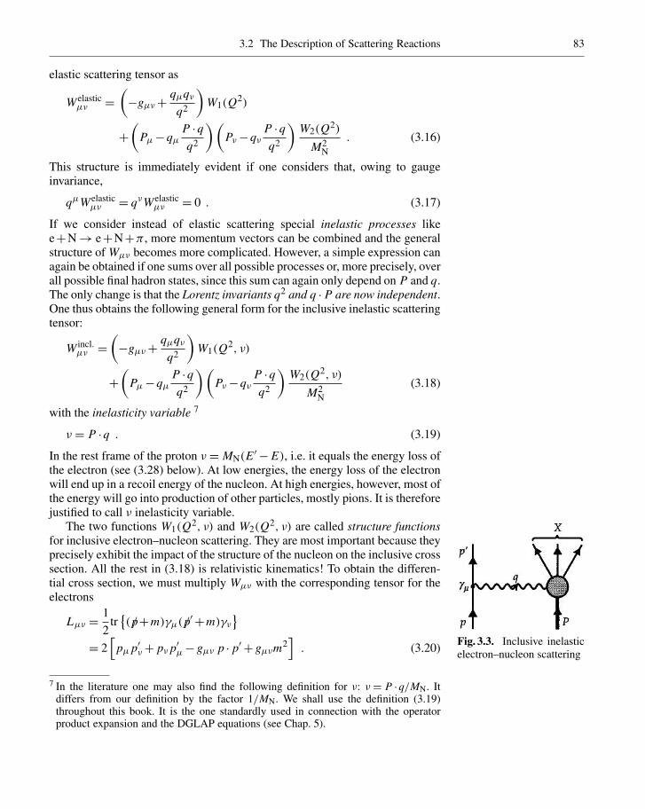
3.2 The Description of Scattering Reactions 83
elastic scattering tensor as
Welasticµν =
(−gµν+ qµqν
q2
)W1(Q
2)
+(
Pµ−qµP ·qq2
)(Pν−qν
P ·qq2
)W2(Q2)
M2N
. (3.16)
This structure is immediately evident if one considers that, owing to gaugeinvariance,
qµWelasticµν = qνWelastic
µν = 0 . (3.17)
If we consider instead of elastic scattering special inelastic processes likee+N → e+N+π, more momentum vectors can be combined and the generalstructure of Wµν becomes more complicated. However, a simple expression canagain be obtained if one sums over all possible processes or, more precisely, overall possible final hadron states, since this sum can again only depend on P and q.The only change is that the Lorentz invariants q2 and q · P are now independent.One thus obtains the following general form for the inclusive inelastic scatteringtensor:
W incl.µν =
(−gµν+ qµqν
q2
)W1(Q
2, ν)
+(
Pµ−qµP ·qq2
)(Pν−qν
P ·qq2
)W2(Q2, ν)
M2N
(3.18)
with the inelasticity variable 7
ν = P ·q . (3.19)
In the rest frame of the proton ν = MN(E′ − E), i.e. it equals the energy loss ofthe electron (see (3.28) below). At low energies, the energy loss of the electronwill end up in a recoil energy of the nucleon. At high energies, however, most ofthe energy will go into production of other particles, mostly pions. It is thereforejustified to call ν inelasticity variable.
The two functions W1(Q2, ν) and W2(Q2, ν) are called structure functionsfor inclusive electron–nucleon scattering. They are most important because theyprecisely exhibit the impact of the structure of the nucleon on the inclusive crosssection. All the rest in (3.18) is relativistic kinematics! To obtain the differen-tial cross section, we must multiply Wµν with the corresponding tensor for theelectrons
Lµν = 1
2tr(p/+m)γµ(p/′ +m)γν
= 2
[pµ p′ν+ pν p′µ− gµν p · p′ + gµνm
2]. (3.20)
7 In the literature one may also find the following definition for ν: ν = P ·q/MN. Itdiffers from our definition by the factor 1/MN. We shall use the definition (3.19)throughout this book. It is the one standardly used in connection with the operatorproduct expansion and the DGLAP equations (see Chap. 5).
Fig. 3.3. Inclusive inelasticelectron–nucleon scattering

84 3. Scattering Reactions and the Internal Structure of Baryons
Equation (3.20) can be obtained by setting A = 1, B = 0 in (3.12). (The factor 12
comes from averaging over the spin directions of the incoming electrons.) Theother factors appearing are the coupling constant and the photon propagator(
e2
q2
)2
= e4
Q4 . (3.21)
Finally, this must be multiplied with normalization and phase-space factors(cf. Example 3.1). The final expression for unpolarized electron–nucleon scat-tering in the laboratory system is
d2σ
dE′dΩ= E′α2
EQ4 LµνWµν . (3.22)
Here E and E′ are defined by
pµ = (E, p) ,
p′µ = (E′, p′) , (3.23)
and the electron mass has been neglected (the extremely relativistic approxima-tion).
Substituting (3.18) and (3.20) into (3.22), this yields
d2σ
dE′dΩ= E′α2
EQ4 2(2pµ pν− gµν p · p′) (3.24)
×[(
−gµν+ qµqνq2
)W1+
(Pµ−qµ
P ·qq2
)(Pν−qν
P ·qq2
)W2
M2N
].
Because qµWµν = 0, we were able to replace p′µ = pµ−qµ by pµ, and we haveagain neglected the electron mass in comparison with pµ and p′µ. We shall set itto zero in the following. Taking into account that
−Q2 = q2 ≈−2 p · p′ (3.25)
and
2 p ·q = 2 p · (p− p′)= 2m2−2 p · p′ ≈ −Q2 , (3.26)
we obtain
d2σ
dE′dΩ= E′
E
α2
Q4 2
[(2(p ·q)2
q2 +3 p · p′)
W1+2
(P · p− q · p
q2 q · P
)2 W2
M2N
−(
Pµ−qµq · P
q2
)2
p · p′ W2
M2N
]
= E′
E
2α2
Q4
[Q2W1+2
(P · p− 1
2P ·q
)2 W2
M2N
−Q2
2
(M2
N−(P ·q)2
q2
)W2
M2N
]. (3.27)

3.2 The Description of Scattering Reactions 85
Let us look at the scattering in the laboratory system, in which the nucleon is atrest before the collision, i.e.,
Pµ = (MN, 0), ν = P ·q = P · (p− p′)= MN(E− E′) . (3.28)
In addition we introduce the scattering angle θ of the electron in the laboratorysystem; thus
p · p′ = |p| |p′| cos(θ)= EE′ cos(θ) (3.29)
and
Q2 = 2 p · p′ = 2(EE′ − p · p′)= 4EE′ sin2(θ
2
). (3.30)
Finally we use definition (3.19):
d2σ
dE′dΩ=E′
E
α2
Q4 2
4EE′ sin2
(θ
2
)W1+2M2
N
(E− ν
2MN
)2 W2
M2N
−[
2EE′ sin2(θ
2
)+ ν2
2M2N
]W2
=E′
E
α2
Q4 2
4EE′ sin2
(θ
2
)W1
+[
2E2−2E(E− E′)−2EE′ sin2(θ
2
)]W2
. (3.31)
Because ν = (P ·q)= (P · p− P · p′)= MN(E− E′), the last term simplifies togive
2M2N EE′
[1− sin2
(θ
2
)]W2
M2N
= 2EE′ cos2(θ
2
)W2 , (3.31a)
and we obtain
d2σ
dE′dΩ
∣∣∣∣eN= 4E′2α2
Q
[2 sin2
(θ
2
)W1
(Q2, ν
)+ cos2
(θ
2
)W2
(Q2, ν
)].
(3.32)
This is the final expression for the inclusive unpolarized electron–nucleonscattering cross section. As mentioned before, the functions W1
(Q2, ν
)and
W2(Q2, ν
)are called the structure functions of inclusive electron–nucleon scat-
tering. To avoid confusion, we write them in what follows as WeN1
(Q2, ν
)and
WeN2
(Q2, ν
). Experimentally one measures for a definite electron beam energy
the direction and energy of the scattered electrons and sums the total reac-tion cross section for each (θ, E′) bin. From this one obtains WeN
1
(Q2, ν
)and
WeN2
(Q2, ν
).

86 3. Scattering Reactions and the Internal Structure of Baryons
What now is the advantage of (3.32)? So far we have only managed to elimi-nate one of the three parameters E, E′, and θ. While d2σ/dE′dΩ can in generalbe any function of E, E′, and θ, we have to express it by arbitrary functions of Q2
and ν. The importance in (3.32) lies mainly in the fact that the structure functionsW1
(Q2, ν
)and W2
(Q2, ν
)can be calculated from the microscopic properties of
the quark model and that then the variables x = Q2/2ν (see (3.39) below) andQ2 are the relevant ones. In the leading order of αs the structure functions turnout to be Q2 independent. Only a very tiny Q2 dependence is observed. This re-sidual Q2 dependence can be used, however, as a most sensitive test for the quarkinteraction, i.e., for QCD.
WeNµν can be expressed by
WeNµν (P, q)= 1
2π
∫d4x eiq·x 1
2
∑pol.
〈N(P)| Jµ(x) Jν(0)|N(P)〉 , (3.33)
where |N(P)〉 designates the state vector of a nucleon with momentum P and Jthe electromagnetic current operator. The derivation of this relation will begiven in Example 3.2.
In the laboratory frame Pµ = (M, 0). Also, we can orient the coordinatesystem such that q points in the z direction. Then from (3.18) it holds that
WeN00 =
(q0q0
q2 −1
)WeN
1
(Q2, ν
)+(
1+ ν
Q2 q0
)2
WeN2
(Q2, ν
)(3.34)
and
WeN11 = WeN
1
(Q2, ν
)(3.34a)
with
q0 = E− E′ = ν/MN . (3.35)
For WeN1
(Q2, ν
)one has according to (3.33):
WeN1
(Q2, ν
)= 1
2π
∫d4x eiq·x 1
2
∑pol.
〈N(P)| J1(x) J1(0)|N(P)〉 . (3.36)
The right-hand side can (at least in principle) be computed for any quarkmodel, and its correctness can thus be tested by comparing the result with theexperimental values for WeN
1 and WeN2 .
We shall illustrate the calculation and the meaning of the nucleon structurefunctions for a very simple, but inadequate, model in Exercise 3.9. This modelis indeed so simple that we do not need to use (3.36) but can choose a simplerway to calculate WeN
1
(Q2, ν
).
Before we discuss the experimentally determined properties of structurefunctions and their meaning, we give the analogous result for neutrino–nucleon

3.2 The Description of Scattering Reactions 87
and antineutrino–nucleon scattering. These formulas again hold in the restsystem of the nucleon, i.e., in the laboratory system:
d2σ
dE′dΩ
∣∣∣∣νN= G2
F
2π2 E′2[
2 sin2(θ
2
)WνN
1
(Q2, ν
)+ cos2
(θ
2
)WνN
2
(Q2, ν
)− E+ E′
MNsin2
(θ
2
)WνN
3
(Q2, ν
)], (3.37)
d2σ
dE′dΩ
∣∣∣∣νN= G2
F
2π2 E′2[
2 sin2(θ
2
)W νN
1
(Q2, ν
)+ cos2
(θ
2
)W νN
2
(Q2, ν
)+E+ E′
MNsin2
(θ
2
)W νN
3
(Q2, ν
)]. (3.38)
Here GF is the Fermi coupling constant of weak interactions. The derivation ofthese relations is to be found in Exercises 3.3 and 3.4.
An important assumption we have made tacitly up to now is that single-photon and single-W exchange dominate the cross section. This assumption issafe because of the smallness of the coupling constants. For strongly interact-ing particles the situation becomes more complicated. Such reactions will beanalyzed in detail in Chap 6.
EXAMPLE
3.1 Normalization and Phase Space Factors
We start with the relation (see (2.116))
dσ = 1
4Eω|v |1
2
∑s,s′
|Fss′ |2 (2π)4 δ4(k′ + p′ − k− p)d3k′
(2π)32ω′d3 p ′
(2π)32E′ ,
(1)
where (E, p ), (E′, p ′), (ω, k) and (ω′, k′) denote the four-momenta of theincoming electron, the outgoing electron, the incoming nucleon, and the out-going multihadron state, respectively. Now we have to integrate this expressionover k′ and, in contrast to elastic electron–pion scattering (see Exercise 2.9), alsoover ω′, since ω′ is no longer fixed by k′. In elastic e–N scattering k′2 =m2
N . Ininelastic e–N scattering, however,
k′2 = (k+ (p− p′))2 = (k+q)2 ≥ m2N ,
i.e., the outgoing nucleon is no longer on the mass shell. Therefore, the energy ω′of the outgoing nucleon becomes an independent variable. Inelasticity opens, soto speak, a new degree of freedom (see Figure 3.3a). Hence (1) becomes
dσ = d3 p ′
4EE′ |v|∫
d4k′⎛⎝1
2
1
4ωω′∑s,s′
|Fss′ |2⎞⎠ (2π)−2 δ4(k′ + p′ − k− p) .
(2)
Fig. 3.3a. Inelastic scatter-ing process. The nucleonfragments into a baryon anda number of pions.

88 3. Scattering Reactions and the Internal Structure of Baryons
Example 3.1 Obviously, the dimension of the integrals has changed by one, implying that thestructure function has got an additional dimension of 1/energy. This is why weshall later on define the dimensionless structure function F1 as F1 = W1 MN. Theintegral on the right-hand side is equal to e4LµνWµν/Q4. Note that the nucleonnormalization factors 2ω and 2ω′ are included in Wµν (see (3.11)) and that Lµνcontains the factor 1/2, which is due to spin averaging (see (3.20)). Thus (2) canbe written as
dσ = d3 p ′
4EE′ |v|e4
(2π)2 Q4 LµνWµν . (3)
For our case (a massless electron incident on a resting nucleon)
|v| ≈ c= 1 . (4)
Furthermore we employ
d3 p′ = (p ′)2 d∣∣p ′∣∣ dΩ′ ≈ E′2dE′ dΩ (5)
and in this way obtain (3.22):
d2σ
dE′dΩ= E′
E
e4
(4π)2 Q4 LµνWµν = E′
E
α2
Q4 LµνWµν . (6)
Comparing with (2) we find
LµνWµν =∫
d4k
(2ω′)(2π)3
(1
4ω
)∑s,s′
∣∣Fs,s′∣∣2 (2π)3δ4(k′ + p′ − k− p) ,
(7)
where we factored out the photon propagator and the elementary charges∣∣Fs,s′∣∣2 = e4
Q4
∣∣Fs,s′∣∣2. The integral
∫d4k/(2ω′)(2π)3 corresponds to a complete
sum∑
X,PXover the outgoing multihadron state, and the delta function will be
absorbed in the definition of the hadronic tensor (see (4) of Example 3.2).
EXAMPLE
3.2 Representation of Wµν by Electromagnetic Current Operators
The coupling of the exchanged photon to the nucleon can be written in a generalway as
Jµ(x)Aµ(x) , (1)
where for the moment no assumption about the structure of Jµ(x) has been made.Now we consider the corresponding current matrix element between the initial

3.2 The Description of Scattering Reactions 89
nucleon state with momentum Pµ and an arbitrary hadronic final state X withfour-momentum PX,µ:⟨
X(PX)
∣∣∣ Jµ(x)∣∣∣N(P)⟩= ⟨
X(PX)
∣∣∣ Jµ(0)∣∣∣N(P)⟩
e−i(P−PX)·x . (2)
In order to evaluate the inclusive cross section, (2) is squared and summed overall X states:∑
X,PX
⟨N(P)
∣∣∣ Jµ(0)∣∣∣X(PX)⟩ ⟨
X(PX)
∣∣∣ Jν(0)∣∣∣N(P)⟩. (3)
In addition we have to average the spin of the incoming nucleon, since thisquantity is not observed. Finally energy-momentum conservation is ensured bya δ function, which is due to the integration over x:
Wµν = 1
2
∑pol.
∑X,PX
⟨N(P)
∣∣∣ Jµ(0)∣∣∣X(PX)⟩ ⟨
X(PX)
∣∣∣ Jν(0)∣∣∣N(P)⟩
× (2π)3 δ4(PX − P−q) . (4)
q denotes the momentum of the virtual photon (see Fig. 3.3a). The δ func-tion arises from the transition amplitude for the scattering process, which isproportional to∫
d4 yd4x Jµe (y)e−iq·(x−y)
q2 JµN (x) ,
where Jµe (y) and JµN (x) represent the electron and nucleon transition currents,respectively. The latter one, which is in fact explicitly given by (2), also revealsits x dependence. The x integration then yields∫
d4xe−iq·xe−i(P−PX )·x = (2π)4δ4(PX − P−q) .
Squaring the amplitude implies also a squaring of the δ function, which yieldsin the well-known way
[(2π)4δ4(PX − P−q)
]2 = (2π)4δ4(PX − P−q)VT ,where VT is the space–time normalization volume which drops out when thetransition rate and cross section are finally calculated. At the end of Example 3.1above we indicated that the factor (2π)3 occurs instead of the usual factor (2π)4
in the definition of the structure function. The summation of the projection op-erator |X(PX)〉〈X(PX)| in (4) has the form of a complete projection operator.But the completeness relation cannot be employed yet, since the argument of theδ function depends on PX .
Using the integral representation
δ4(PX− P−q)=∫
d4y
(2π)4e−i(PX−P−q)·y , (5)
Example 3.2

90 3. Scattering Reactions and the Internal Structure of Baryons
Example 3.2 we can write (4) in the form
Wµν = 1
2
∑pol.
∑X,PX
1
2π
∫d4y
⟨N(P)
∣∣∣ Jµ(0)∣∣∣X(PX)⟩
×⟨X(PX)
∣∣∣ Jν(0)∣∣∣N(P)⟩
e−i(PX−P)·y eiq·y
= 1
4π
∑pol.
∑X,PX
∫d4y
⟨N(P)
∣∣∣ Jµ(y)∣∣∣X(PX)⟩ ⟨
X(PX)
∣∣∣ Jν(0)∣∣∣N(P)⟩
eiq·y,
(6)
where Jµ(y) has been obtained by means of (2). Now we are able to employ thecompleteness relation∑
X,PX
|X(PX)〉〈X(PX)| = 1 , (7)
which yields the expression for Wµν(P, q) given in (3.33):
Wµν(P, q)= 1
4π
∑pol.
∫d4y eiq·y ⟨N(P) ∣∣∣ Jµ(y) Jν(0)∣∣∣N(P)
⟩. (8)
Now it is interesting to note that instead of the operator product Jµ(y) Jν(0) alsothe expectation value of the commutator of the current operators could be usedin (8), i.e.,
Wµν = 1
4π
∑pol.
∫d4y eiq·y ⟨N(P) ∣∣∣[ Jµ(y) Jν(0)
]∣∣∣N(P)⟩. (9)
In order to show the equivalence of (8) and (9) one has to prove that the followingexpression vanishes:∫
d4y eiq·y ⟨N(P) ∣∣∣ Jν(0) Jµ(y)∣∣∣N(P)⟩
=∑X,PX
∫d4y eiq·y ⟨N(P) ∣∣∣ Jν(0)∣∣∣X(PX)
⟩ ⟨X(PX)
∣∣∣ Jµ(y)∣∣∣N(P)⟩
=∑X,PX
∫d4y ei(q+PX−P)·y ⟨N(P) ∣∣∣ Jν(0)∣∣∣X(PX)
⟩ ⟨X(PX)
∣∣∣ Jµ(0)∣∣∣N(P)⟩
= (2π)4∑X,PX
δ4(PX− P+q)⟨N(P)
∣∣∣ Jν(0)∣∣∣X(PX)⟩ ⟨
X(PX)
∣∣∣ Jµ(0)∣∣∣N(P)⟩.
(10)
The energy δ function requires that EX = P0−q0 = MN− (E− E′) < MNholds in the lab system. However, such a state X does not exist, since the nucleonis the state of lowest energy with baryon number 1. Therefore (10) vanishes and(9) is proved.

3.2 The Description of Scattering Reactions 91
EXERCISE
3.3 The Nucleonic Scattering Tensor with Weak Interaction
Problem. Repeat the discussion leading from (3.6) to (3.18) assuming that par-ity is not conserved, i.e., that Γµ consists of Lorentz vectors and Lorentz axialvectors. Take into account that time-reversal invariance still holds.
Solution. Have a look at Fig. 3.2. We are again discussing the elastic process de-scribed by that figure, but allow for non-parity-conserving currents. In this casethe transition current is of the general form
u(P′)Γµu(P)= B(P′µ+ Pµ)S+ iC(P′µ− Pµ)S+ A Vµ+D(P′ν+ Pν)Tµν+ iE(P′ν− Pν)Tµν+ B′(P′µ+ Pµ)P+ iC′(P′µ− Pµ)P+ A′ Aµ
+D′(P′ν+ Pν) εµναβ Tαβ+ iE′(P′ν− Pν) εµναβ Tαβ (1)
with real functions A, B, C, . . . and with
S = u(P′) u(P) scalar ,
P = u(P′) i γ5 u(P) pseudoscalar ,
Vµ = u(P′) γµ u(P) vector ,
Aµ = u(P′) γµ γ5 u(P) pseudovector ,
Tµν = u(P′) σµν u(P) tensor . (2)
In (1) we have assumed that the transition current is real, i.e.(u(P′) Γµ u(P)
)† = u(P′) Γµ u(P)
and therefore
u†(P)γ0 γ0Γ†µγ0u(P′)= u(P)Γµu(P′) .
Here the relation γ 0Γ†µγ
0 = Γµ was used, which can easily be verified in thestandard representation of the γµ and σµν = i
2
[γµ, γν
]. Obviously, the exchange
P ↔ P′ should have the same effect as complex conjugation. In other words, theright-hand side must therefore be invariant under the transformation
(· · · )∗∣∣P′µ↔Pµ. (3)
Time inversion yields (see Table 2.1)
S → S , P →−P , Vµ→ Vµ , Aµ→ Aµ , Tµν →−Tµν , (4)
and
P ↔−P′ , P0 ↔ P′0 , i.e. Pµ↔ P′µ . (5)

92 3. Scattering Reactions and the Internal Structure of Baryons
Exercise 3.3 The transition P ↔−P′, P0 ↔ P′0 is due to the complex conjugation ofu(P′) Γµ u(P), which replaces the momentum P′µ by the negative value of Pµand vice versa, i.e., P′µ↔−Pµ. Because t →−t there is an additional change inthe sign of the zero component. This is easily understood, because under time re-versal the direction of motion changes and initial and final states are exchanged.The energies, however, remain positive.
Under combined transformations (4) and (5), (1) assumes the form
u(P′)Γµu(P)→B(P′µ+ Pµ)S− iC(P′µ−Pµ)S+ A Vµ−D(P′ν+ Pν)Tµν
+ iE(P′ν− Pν)Tµν− B′(P′µ+ Pµ)P+ iC′(P′µ− Pµ)P+ A′ Aµ
−D′(P′ν+ Pν) εµναβ Tαβ+ iE′(P′ν− Pν) εµναβ Tαβ . (6)
Only the spatial components of the current vector should change sign undertime reversal. In order to conserve T invariance (6) must therefore be equalto u(P′) Γ µ u(P). For the ε tensor the relation εµναβ =−εµναβ holds. Thiscan be verified from the definition −4iεµναβ = tr
[γ5γµγνγαγβ
]. The indices
µ, ν, α, β have to be 0, 1, 2, 3, and different from each other. Now−4iε0,1,2,3 =tr[γ5γ
0γ 1γ 2γ 3]=−tr [γ5γ0γ1γ2γ3]=+4iε0,1,2,3. For different permutations
of 0, 1, 2, 3 the analogous relation holds. Employing now εµναβ =−εµναβ wehave
C = D = B′ = E′ = 0 . (7)
Because of the Gordon decomposition (see earlier text and (3.10)), E can againbe replaced by A and B. In an analogous way D′ can also be eliminated using A′and C′. In order to derive this identity we consider the expression
u(P′)(−2MNa/γ5+
P/′ − P/
2, a/
+γ5+
[P/′ + P/
2, a/
]−γ5
)u(P)
= u(P′)(−2MNa/γ5+ P/′a/γ5−a/P/γ5
)u(P)
= u(P′) (−2MNa/γ5+MNa/γ5+a/γ5 MN) u(P)
= 0 . (8)
Differentiating this relation with respect to aµ yields
∂
∂aµaαγα = δαµγα = γµ
and we obtain
u(P′)(−2MNγµγ5+ (P′ − P)λ
1
2
γλ, γµ
γ5
+ (P′ + P)λ1
2
[γλ, γµ
]γ5
)u(P) . (9)

3.2 The Description of Scattering Reactions 93
With (1/2)γλ, γµ
= gλ,µ and (1/2)[γλ, γµ
]=−iσλ,µ and with (8) we there-fore conclude that
0 =−2MN Aµ+ u(P′)[(P′µ− Pµ)γ5− i(P′ν+ Pν)σνµ γ5
]u(P)
=−2MN Aµ− i(P′µ− Pµ)P− 1
2εµναβ Tαβ(P′ν+ Pν) , (9b)
which represents the desired result. Consequently we have reduced (1) to
u(P′)Γµu(P)= B(P′µ+ Pµ)S+ A Vµ+ iC′(P′µ− Pµ)P+ A′Aµ . (10)
Here the letters B, A, C′, and A′ denote constants while S, Vµ, P, and Aµ standfor the various currents denoted in (2). Similarly, as in (3.11), Wµν then becomes
Wµν = tr
[Aγµ+ B(P′
µ+ Pµ)
+ A′γµγ5+C′(P′µ− Pµ)γ5)
](P/′ +MN)
[Aγν+ B(P′
ν+ Pν)
+ A′γνγ5−C′(P′ν− Pν)γ5
](P/+MN)
= tr
[Aγµ+ B(P′
µ+ Pµ)](P/′ +MN)
[Aγν+ B(P′
ν+ Pν)](P/+MN)
+ tr
[A′γµ+C′(P′
µ+ Pµ)](−P/′ +MN)
[−A′γν−C′(P′ν− Pν)
](P/+MN)
+ tr
A′γµγ5 P/′AγνP/+ AγµP/′A′γνγ5 P/
. (11)
Note again that we have used the normalization for the u and v spinors expressedin (2.50). The first two traces do not have to be evaluated explicitly. It is sufficientto know that because P′µ = qµ+ Pµ their contribution can only be of the form
gµνV1+ PµPνV2+ (Pµqν+ Pνqµ)V3+qµqνV4 . (12)
In the case of the last trace the identity
trγ5a/b/c/d/
= 4iεµναβ aµ bν cα dβ
holds. Therefore the hadronic tensor is of the form
Wµν = gµνV1+ PµPνV2+ (Pµqν+ Pνqµ)V3+qµqνV4+ iεµναβPαqβV5 .
(13)
We have derived (13) for elastic lepton–nucleon scattering. In the case of inelas-tic processes, including particle creation, qµ = P′µ− Pµ is no longer valid. q · P′,q2 and q · P are then independent quantities. However, the results again are quitesimple if one sums over all possible final states, i.e., over the final states of thereactions
νe(p)+N(P)→ e−(p−q)+X ,
νe(p)+N(P)→ e+(p−q)+X . (14)
Exercise 3.3

94 3. Scattering Reactions and the Internal Structure of Baryons
Exercise 3.3
Fig. 3.3b. Deep inelasticscattering with charged vec-tor bosons.
Therefore the inclusive inelastic scattering tensor for parity-violating lepton–nucleon scattering is
Wµν = gµνV1(Q2, ν)+ PµPνV2(Q
2, ν)+ (Pµqν+ Pνqµ)V3(Q2, ν)
+qµqνV4(Q2, ν)+ iεµναβPαqβV5(Q
2, ν) . (15)
EXERCISE
3.4 The Inclusive Weak Lepton–Nucleon Scattering
Problem. The coupling of the charged vector bosons W±µ of the weak interac-
tion to leptons is described by the interaction Lagrangean (4.23),
L int = +g√2Ψf(T−W+
µ + T+W−µ )γ
µΨf , (1)
where Ψf =(νee
)L denotes the doublet of the left-handed electron–neutrino
field: eL = 1−γ52 eL. Writing (1) we have used T± = 1√
2
(λ12 ± iλ2
2
). With T− =(
0 01 0
)and T+ =
(0 10 0
)we get for the fundamental (e, ν) interaction
+g√2ν(x)γµ
1−γ5
2e(x)Wµ(x)+h.c. . (1a)
The corresponding processes are depicted in the figure. Derive from this equationthe leptonic scattering tensor Lµν. Employ the result of Exercise 3.3 to evaluatethe differential cross section for the inclusive weak lepton–nucleon scattering.
Solution. Since the neutrino is massless and the electron mass can be neglected,it is helpful to choose the following spinor normalization.
u†α(p)uβ(p)= 2Eδαβ ,∑spin
u(p)u(p)= p/+m = p/ . (2)
The leptonic scattering tensor is then
Lµν = g2
8
∑s
trν(p)γµ(1−γ5)e(p′, s)e(p′, s)γν(1−γ5)ν(p)
= g2
8tr
p/γµ(1−γ5)p/′γν(1−γ5)
(utilizing (2)))
= g2
4
(tr
p/γµ p/′γν− tr
γ5 p/′γν p/γµ
)= g2
(p′µ pν+ pµ p′ν− p′ · p gµν− iεµναβ pα p′β
). (3)

3.2 The Description of Scattering Reactions 95
Since the neutrino is always left-handed, there is no averaging of the initialspin. Nevertheless, in order to obtain the trace in the second line of (3) we havesummed over all neutrino spins and made use of (2). This procedure is correct,because the operator (1−γ5) cancels the contribution of the nonphysical right-handed neutrino state. In analogy to (3.22) the differential cross section thenbecomes
d2σ
dE′ dΩ= E′
(4π)2 E
(1
q2−M2W
)2
Lµν(
g√2
)2
Wµν . (4)
The differences can be explained as follows.
(1) The propagator for massive W bosons differs from that for massless photons.For |q2| M2
W we can use(1
q2−M2W
)2
≈ 1
M4W
. (5)
This yields Fermi’s theory of weak interaction.(2) The coupling constant of the W bosons to the nucleon is effectively chosento be GF/
√2 where GF = g2/(4
√2M2
W) is the Fermi constant of weak interac-tion. Since we have already absorbed a factor of g2/8 (see (3)) in the definition ofthe leptonic tensor we are left with a factor of g2/(4 ·2) in front of the hadronictensor Wµν, which according to (3.11) does not contain any coupling constant.(3) The factor 1/(4π)2 arises by replacing α2 = e4/(4π)2 → g4/(4π)2. Onefactor g2 is contained in Lµν, the other one appears explicitly in (4).
In order to evaluate (4) we first show that qµLµν and qνLµν vanish:
qµLµν = g2(q · p′ pν+q · p p′ν− p′ · p qν− iεµναβ qµ pα p′β)
= g2[− q2
2pν+ q2
2p′ν+
q2
2(pν− p′ν)
]= 0 . (6)
Here we have employed
qµ = pµ− p′µ ⇒ p · p′ = −q2
2,
p ·q = q2
2and p′ ·q =−q2
2, (7)
which all hold in the high-energy limit m2 q2. With help of 15 from Exer-cise 3.3 it therefore follows that
LµνWµν = Lµν(gµνV1+ PµPνV2+ iεµναβPαqβV5
)= g2
[(2 p′ · p−4 p′ · p)V1+
(2 p′ · P p · P−M2
N p · p′)V2
+εµναβ εµνδγ pδqγ PαqβV5
]. (8)
Exercise 3.4

96 3. Scattering Reactions and the Internal Structure of Baryons
Exercise 3.4 With
p = (E, p ) , p′ = (E′, p ′ ) , P = (M, 0 ) , (9)
and8
εµναβ εµνδγ =−2
(gαδ gβγ − gαγ gβδ
), (10)
and, also, utilizing relations (7) this assumes the form
LµνWµν = g2[
q2V1+M2N
(2EE′ + 1
2q2)
V2−2(
p · P q2− P ·q p ·q)
V5
]= g2
q2V1+2M2
N
(EE′ + 1
4q2)
V2−2MN
[Eq2− (E− E′)q2
2
]V5
.
(11)
Again, using (3.30), we find that
q2 =−Q2 =−4EE′ sin2(ϑ
2
)(12)
leads to
LµνWµν = g22EE′[−2 sin2
(ϑ
2
)V1+M2
N cos2(ϑ
2
)V2
+2MN sin2(ϑ
2
)(E+ E′)V5
]. (13)
In order to provide all structure functions with the same dimension we define
W1 =−V1 , W2 = V2 M2N , W3 =−2V5 M2
N (14)
and obtain
d2σ
dE′dΩ= E′2g4
4M4W(4π)
2
[2 sin2
(ϑ
2
)W1(Q
2, ν)+ cos2(ϑ
2
)W2(Q
2, ν)
− E+ E′
MNsin2
(ϑ
2
)W3(Q
2, ν)
]. (15)
Finally we substitute the so-called Fermi constant of weak interaction:
GF = g2
4√
2M2W
; (16)
8 The proof of this relation can be found in Exercise 2.4 of W. Greiner and B. Müller:Gauge Theory of Weak Interactions, 3rd ed. (Springer, Berlin, Heidelberg 2000).

3.2 The Description of Scattering Reactions 97
d2σ
dE′dΩ= G2
F E′2
2π2
[2 sin2
(ϑ
2
)W1(Q
2, ν)+ cos2(ϑ
2
)W2(Q
2, ν)
− E+ E′
MNsin2
(ϑ
2
)W3(Q
2, ν)
]. (17)
This is identical to (3.37). In the reaction ν+N → e++X the incoming antineu-trino corresponds to the outgoing electron in the reaction ν+N→ e−+X, i.e.,p and p′ are exchanged. Since the third term in Lµν is antisymmetric under thisexchange, the sign of W3 changes.
We shall now discuss the experimental structure functions of electron–nucleon scattering. These functions will have a particularly simple form whenν is replaced by x = Q2/2ν. This quantity is called the Bjorken or scaling vari-able. We shall first consider some of its properties. For elastic scattering, (3.19)and (3.7) give
x = Q2
2ν= −q2
2P ·q = −q2
−q2 = 1 . (3.39)
Since the nucleon is the lightest state with baryon number 1, we know in additionthat the invariant mass of the final state
MX =√(P+q)2 (3.40)
must be larger than MN. If this were not the case, there would be a state X (ofarbitrary structure) with baryon number 1 into which the proton could decay, byemitting γ quanta, for example.
From (3.40) it follows that x is always positive and less than 1:
x = Q2
(P+q)2− P2+Q2 =Q2
M2X−M2
N+Q2
= 1
1+ (M2X−M2
N)/Q2; (3.41)
Q2 is always positive, as can be seen from (3.30), and
0< x ≤ 1 . (3.42)
Additionally, it is customary to include a factor of ν in the definition of W2 andW3 and a factor of MN in the definition of W1. Thus we are lead to “new” formfactors F1, F2, F3 instead of W1, W2, and W3, respectively:
MNWeN1 (Q2, ν)= FeN
1 (Q2, x) ,ν
MNWeN
2 (Q2, ν)= FeN2 (Q2, x) ,
ν
MNWνN
3 (Q2, ν)= FeN3 (Q2, x) . (3.43)
Exercise 3.4

98 3. Scattering Reactions and the Internal Structure of Baryons
Fig. 3.4. The physical mean-ing of the different domainsof x, Q2, and ν. Q2 = 2Mν
holds for elastic scatteringonly, otherwise Q2 and ν areindependent
Frequently, also the parameter Q2 is replaced by a new quantity, the inelasticityparameter y:
y = ν
MN E= E− E′
E. (3.44)
y is dimensionless and specifies which fraction of the lepton energy in the labo-ratory system is transferred to the nucleon. The value of y thus lies in the range0 ≤ y ≤ 1. The meaning of Q2, ν, and x is also illustrated in Fig. 3.4. It can easilybe checked (see Exercise 3.5) that
d2σ
dE′dΩ= E′
2πMN Ey
d2σ
dxdy. (3.45)
In this notation, (3.32) becomes (see Exercise 3.5):
d2σ
dx dy
∣∣∣∣eN= 8πMN Eα2
Q4
×[
xy2 FeN1 (Q2, x)+
(1− y− MNxy
2E
)FeN
2 (Q2, x)
]. (3.46)
The first measurements of inelastic electron–proton scattering at high energieswere performed in 1968 at the Stanford Linear Accelerator (SLAC). These andsubsequent experiments have yielded two important results:
(1) For sufficiently large values of Q2, i.e., for Q2 ≥ 1GeV2, FeN2 and FeN
1 donot depend significantly on Q2, but only on x. This behavior is termed Bjorkenscaling.
(2) In this domain (i.e., for Q2 ≥ 1GeV2) it holds to good approximation that
FeN2 ≈ 2xFeN
1 .

3.2 The Description of Scattering Reactions 99
EXERCISE
3.5 The Cross Section as a Function of x and y
Problem. Derive (3.45) and (3.46).
Solution. Equations (3.44), (3.39), and (3.30) yield
y = E− E′
E= 1− E′
E,
x = Q2
2(E− E′)MN= 2EE′
(E− E′)MNsin2
(θ
2
). (1)
Owing to the cylindrical symmetry of the problem we have in addition
d2σ
dE′dΩ= d2σ
dE′2π sin(θ)dθ. (2)
Therefore we only have to evaluate the Jacobi determinant
d2σ
dE′dΩ= 1
2π sin(θ)
∣∣∣∣ ∂(x, y)
∂(E′, θ)
∣∣∣∣ d2σ
dxdy
=∣∣∣∣∣∣
2E sin2(θ
2
)MN
(E′+(E−E′)(E−E′)2
)2EE′
(E−E′)MNsin
(θ2
)cos
(θ2
)− 1
E 0
∣∣∣∣∣∣ 1
2π sin(θ)
d2σ
dxdy
= 1
2π sin(θ)
2E′
(E− E′)MN
sin(θ)
2
d2σ
dx dy
= E′
2πMN Ey
d2σ
dx dy. (3)
This is identical to (3.45). With the help of the definitions introduced in (3.39)–(3.44) the double-differential cross section for electron–nucleon scattering con-sequently becomes
d2σ
dxdy= 8πMNyEE′α2
Q4
[2
MNsin2
(θ
2
)FeN
1 (Q2, x)+cos2(θ2
)yE
FeN2 (Q2, x)
].
(4)
Here we have employed (3.32) and (3.43). Now we replace θ by x and y,using (1):
sin2(θ
2
)= (E− E′)MN
2EE′ x = MN
2E′ xy , (5)

100 3. Scattering Reactions and the Internal Structure of Baryons
Exercise 3.5
Fig. 3.5. The F2 struc-ture functions for electron–proton and electron–neutronscattering have been com-bined into Fep
2 ± Fen2 and
plotted against Q2. TheBjorken variable x is definedas x = Q2/2νMN (see Re-view of Particle Properties:Phys. Lett. 170 (1986))
d2σ
dxdy= 8πMNyEE′α2
Q4
[xy
E′ FeN1 (Q2, x)+ 1− MN
2E′ xy
yEFeN
2 (Q2, x)
]= 8πMN Eα2
Q4
[xy2 FeN
1 (Q2, x)+(
1− y− MN
2Exy
)FeN
2 (Q2, x)
],
(6)
which yields (3.46).
These results are illustrated in Figs. 3.5 and 3.6. In Fig. 3.5 it can be seen that,at least for medium values of x, the measured points are practically horizontal. Inthe following we shall discuss the physical meaning of this. In Chap. 5 we shalldiscuss how the Q2 dependence of the structure functions for large and small xcan be understood in the framework of quantum chromodynamics.
These two unusual properties can be easily reduced to the common physi-cal cause that the scattering is off pointlike spin- 1
2 constituents of the nucleon.These constituents are termed, following R.P. Feynman, partons. What do weknow about this kind of scattering?
The scattering cross section dσi/dΩ for the scattering of electrons offa pointlike parton of mass Mi and charge qie can be constructed from the re-

3.2 The Description of Scattering Reactions 101
sults for electron–muon scattering, namely (2.173), (see in particular 11 inExercise 2.13), which now reads
dσi
dΩ= α2q2
i
4E2 sin4 θ/2
E′
Ecos2 θ/2
(1− q2 tan2 θ/2
2M2i
)
= α2q2i
4E2
E′
E
1
sin4 θ/2
[cos2 θ/2+ Q2
4M2i
sin2 θ/2
].
From
2(E− E′) M = 2ν = Q2 =+4EE′ sin2
(θ
2
),
one findsE
E′ = 1+ 2E
Msin2
(θ
2
),
and therefore
dσi
dΩ= α2q2
i
4E2 sin4(θ2
) 1
1+ 2EMi
sin2(θ2
) cos2(θ
2
)[1− q2 tan2
(θ2
)2M2
i
]
= α2q2i
4E2
1
sin4(θ2
)[
cos2(θ2
)− q2
2M2i
sin2(θ2
)]1+ 2E
Misin2
(θ2
) . (3.47)
This cross section is computed in the laboratory system as the rest system of theparton. The laboratory system, however, is quite unsuitable for our needs sincehere partons cannot be treated as free particles because they are held together bythe interaction to which this volume is dedicated. Thus we do not know at all theinitial momenta of the partons; they are definitely not at rest. There are, however,frames of reference where the initial momentum is known. These are all framesof reference in which the nucleon is moving very fast. The momentum of the ithparton is then
Pi,µ = ξi · Pµ+∆Piµ , maxµ(∆Pµ)max
µ(Pµ) . (3.48)
Here maxµ(∆Pµ) stands for the maximum of ∆Pµ for the various space–timecomponents µ. The unknown momentum fraction∆Piµ′ , which comes from theinteractions of the partons with each other, is much smaller than the momen-tum from the collective motion. To describe electron–parton scattering sensibly,(3.47) must be transformed into a different Lorentz system.9 This is done byrewriting it using only the invariant variables
(p− p′)2 =: t =−Q2 = (P− P′)2 ,(p+ P)2 =: s = (p′ + P′)2 ,(p′ − P)2 =: u = (p− P′)2 . (3.49)
9 Here and in the following we omit the parton index i on the mass and momentumvariables.

102 3. Scattering Reactions and the Internal Structure of Baryons
These quantities are called Mandelstam variables. In the laboratory system
Q2 = 4EE′ sin2(θ
2
), (3.50a)
s = 2 p · P+M2 = M(2E+M) , (3.50b)
u =−2 p′ · P+M2 =−M(2E′ −M) . (3.50c)
The small mass of the electron (m2 M2, p · P) has been neglected here. Q2 issolely a function of θ, because the E′ appearing in (3.50a) can be expressed interms of E and θ (see (3.53) below). Therefore we may use (note the cylindricalsymmetry)
dσ
dΩ= 1
2π
dσ
sin(θ)dθ= 1
2π sin(θ)
dQ2
dθ
dσ
dQ2 . (3.51)
From P′µ = Pµ+ pµ− p′µ, it follows that
M2 = P′2µ = (Pµ+ pµ− p′µ)2 = M2+ (2E− E′)M−Q2 , (3.52)
or, after solving for E′,
E′ = E
[1+2
E
Msin2
(θ
2
)]−1
. (3.53)
For the derivative dQ2/dθ we obtain, with (3.50a) and (3.53),
dQ2
dθ= 4EE′ sin
(θ
2
)cos
(θ
2
)− E 2 E
M sin(θ2
)cos
(θ2
)[1+2 E
M sin2(θ2
)]2 4E sin2(θ
2
)
= 2EE′ sin θ
1− 2E sin2
(θ2
)M[1+2 E
M sin2(θ2
)]
= 2EE′ sin θ[1+2 E
M sin2(θ2
)] . (3.54)
For dσ/dQ2 we therefore find according to (3.51) and (3.47) that
dσ
dQ2 =2π sin2
dQ2
dθ
dσ
dω
= π
EE′α2q2
i
4E2
1
sin4(θ2
) [cos2(θ
2
)+ Q2
2M2i
sin2(θ
2
)]. (3.55)

3.2 The Description of Scattering Reactions 103
We further insert, according to (3.50),
E′ = u−M2i
−2Mi, E = s−M2
i
2Mi,
sin2(θ
2
)= Q2
4EE′ = − Q2 M2i(
u−M2) (
s−M2i
) ,cos2
(θ
2
)= 1+ Q2 M2
i(u−M2
i
) (s−M2
i
) , (3.56)
so that after appropriate substitutions, (3.55) becomes
dσi
dQ2 =4πα2q2
i
Q4
×(−ui −M2
i
si −M2i
)[1+
(1− Q2
2M2i
)Q2 M2
i(ui −M2
i
) (si −M2
i
)] . (3.57)
The quantities ui and si refer to the ith parton. With this, we have succeeded inthe first step. We must now choose an appropriate laboratory system and sub-stitute the parton masses. It is now a major statement of the parton model thatone obtains a good description of experimental results when one assumes thatpartons are massless. For Mi → 0, (3.57) simplifies to
dσi
dQ2 =4πα2q2
i
Q4
(Q4
2uisi−1
)ui
si. (3.58a)
In addition, from (3.49) one deduces
Q2− si −ui = 2p · p′ −2p · Pi +2p · Pi′
= 2p · (p′ − Pi + Pi′)= 2p2 = 0 (3.59)
and therefore Q4 = s2i +u2
i +2uisi , so that(Q4
2uisi−1
)ui
si= s2
i +u2i
2s2i
. (3.60)
Thus (3.58a) becomes
dσi
dQ2 =4πα2q2
i
Q4
(s2
i +u2i
2s2i
). (3.58b)
For our frame of reference, we now choose the so-called Breit system. Thisis characterized by the property that qµ is purely spacelike and points in thez direction (see Exercise 3.6):
qµ =(
0, 0, 0,√−q2
)=(
0, 0, 0,√
Q2),
Pµ =(P, 0, 0,−P
), P MN , P2 = P2− P2 = 0 ≈ M 2
N . (3.61)

104 3. Scattering Reactions and the Internal Structure of Baryons
Since we neglect the momentum fraction of the partons stemming from theparton–parton interaction, for consistency we must also neglect the nucleonmasses:
Pi,µ = ξi(P, 0, 0,−P
). (3.62)
The cross section for scattering off a parton in the Breit system thus becomes
dσi
dQ2 =4πα2q2
i
Q4
((p+ Pi)
4+ (p′ − Pi)4
2(p+ Pi)4
)= 4πα2q2
i
Q4
((ξi2p · P)2+ (ξi2p′ · P)2
2(2ξi p · P)2
)= 4πα2q2
i
Q4
((p+ P)4+ (p′ − P)4
2(p+ P)4
)= 4πα2q2
i
Q4
(s2+u2
2s2
). (3.63)
s and u are now Mandelstam variables for the whole nucleon. We recognize thatdσ/dQ2 is completely independent of ξi . To compare this expression with (3.46),we must write in the Breit system not only the elastic scattering cross section forpointlike particles, i.e.(3.63) above, but also the inelastic scattering cross sectionfor particles with an internal structure (see (3.46)). To this end, (3.46) is rewrit-ten such that only Lorentz-invariant quantities appear. For M2
N u, s, Q2 (see(3.56))
E′ = − u
2MN, E = s
2MN,
y = E− E′
E≡ s+u
s(3.64)
and
x = Q2
2ν= Q2
2P ·q = Q2
s+u. (3.65)
Equation (3.46) is thus nearly in invariant form. One only has to substitute sfor E:
d2σ
dx dy
∣∣∣∣eN= 4πsα2
Q4
[xy2 FeN
1 (Q2, x)+(
1− y− xyM2N
s
)FeN
2 (Q2, x)
].
(3.66)
Because MN s the second term can be further simplified. This expression mustnow be compared to the sum over partons i of (3.63). To this end, we must firstrewrite (3.63) as a double-differential cross section.
To do this, we start from the momentum conservation P′i = Pi +q for thescattering parton, i.e.,
0 ≈ Pi′2 = (Pi +q)2 = (ξi P+q)2 = ξ2
i M2i +2ξi P ·q+q2 . (3.67)

3.2 The Description of Scattering Reactions 105
When the parton mass vanishes, this implies that
ξi = Q2
2P ·q = x . (3.68)
This is an interesting relation, which allows us to interprete the variable x ina new way: If we observe scattering characterized by a Bjorken variable x, thismeans in the parton model that the interacting parton carried a fraction ξi = x ofthe nucleon’s total momentum! Hence the variable x has a simple meaning (butonly in reference frames with very large nucleon momentum, e.g. in the Breitframe).
Owing to (3.68), (3.63) can immediately be written as a double differential:
d2σ
dx dQ2 =4πα2q2
i
Q4
s2+u2
2s2 δ(ξi − x) . (3.69)
The transition from Q2 to the desired variable y is achieved with the aid of (3.39),(3.44), and (3.56), according to which
Q2 = 2 P ·q x = 2MN(E− E′)x = 2MN Eyx = syx , (3.70)
and we thus obtain
d2σ
dx dy= dQ2
dy
∣∣∣∣x
d2σ
dx dQ2 =2πα2q2
i
Q4
s2+u2
s2 δ(ξi − x)Q2s
s+u. (3.71)
Here, in the last step, we have put x = Q2/(s+u), according to (3.65). To obtainthe total cross section in the parton model, we must sum (3.71) over all partons iand all possible momentum fractions ξi . The single terms of the sum must beweighted with their proper probabilities fi(ξi):
d2σ
dx dy
∣∣∣∣eN=∑
i
1∫0
dξi fi(ξi)2πα2q2
i
Q4
s2+u2
s2 δ(ξi − x)Q2s
s+u
= 2πα2s
Q4
s2+u2
s2
∑i
fi(x)q2i x
(remember x = Q2
s+u
)= 2πα2s
Q4
[(y−1)2+1
]∑i
fi(x)q2i x (3.72)
with
(y−1)2+1 = y2−2y+2 =(
s+u
s
)2
−2s+u
s+2
= s2+u2
s2 + 2su
s2 −2s+u
s+2
= s2+u2
s2

106 3. Scattering Reactions and the Internal Structure of Baryons
according to (3.64). For the momentum distribution functions fi(ξi) of thepartons the normalization
1∫0
dξi fi(ξi)= 1 (3.73)
holds. Comparing (3.72) with (3.66) shows that in the parton model the followingidentification must hold:
2[xy2 FeN
1 (Q2, x)+ (1− y)FeN2 (Q2, x)
]=[(y−1)2+1
]∑i
fi(x)q2i x ,
s = const . (3.74)
This equation (3.74) holds for all scattering processes, i.e., for any value of E,E′, and θ. We use this fact by letting the parameter s = 2MN E, which was fixedup to now, vary:
s → s′ = s′
ss . (3.75)
Simultaneously, we substitute
u → s′
su = u′ , Q2 → s′
sQ2 = Q′2 . (3.76)
x and y are not changed under the simultaneous transformations
y → s′ +u′
s′= s+u
s, x → Q′2
s′ +u′= Q2
s+u, (3.77)
or
y′ = y , x′ = x . (3.78)
Since the right-hand side of (3.74), computed in the parton model, dependsonly on the variables x and y, and is therefore invariant under the scalingtransformations (3.75)–(3.77), it follows for the left-hand side that
xy2 FeN1 (Q2, x)+ (1− y)FeN
2 (Q2, x)= const for all Q2 = Q′2 , (3.79)
which implies that the functions FeN1 (Q2, x) and FeN
2 (Q2, x) do not dependon Q2 at all, i.e.
FeN1 (Q2, x)= FeN
1 (x) , FeN2 (Q2, x)= FeN
2 (x) . (3.80)
The structure functions in the parton picture thus no longer depend on Q2.Since we have neglected here both the momenta coming from the binding ofthe partons and the nucleon mass, (3.79) should hold for sufficiently large valuesfor Q2. This has indeed been experimentally observed as discussed above. It is

3.2 The Description of Scattering Reactions 107
the so-called Bjorken scaling, which we now do understand within the partonmodel. Equation (3.74) then becomes
2[xy2 FeN
1 (x)+ (1− y)FeN2 (x)
]=[
y2+2(1− y)]∑
i
fi(x)q2i x . (3.81)
By comparing powers of y, we find that
FeN1 (x)= 1
2
∑i
fi(x)q2i , FeN
2 (x)=∑
i
fi(x)q2i x , (3.82)
and
FeN2 (x)= 2xFeN
1 (x) . (3.83)
This is the Callan–Gross relation. Moreover, the nucleon form factors are now– within the parton model – simply related to the parton distribution functionsfi(x), describing the distribution of the fraction of the total nucleon momentumshared by the ith parton.
We have thus seen that deep inelastic scattering processes can be explainedby the basic assumptions of the parton model: the hadron is built of pointlikeconstituents whose energy of interaction with each other and whose mass is smallcompared to
√Q2 > 1GeV.
The physical foundations of (3.81) and (3.82) can also be illustrated froma different point of view: we can assume that partons are massless. There areno dimensional quantities in electron–parton scattering except for the momenta.Hence, the only Lorentz-invariant quantities are q2, P2, and P ·q. Now, P2 =M2 = 0, because of the vanishing parton masses. From Q2 =−q2 and P ·q onecan only have Q2 and the dimensionless x = Q2/2P ·q. Since FeN
1 (Q2, x) is
dimensionless, it can only depend on x alone, i.e. FeN1 (Q2, x)= FeN
1 (x).We have already seen that three structure functions are present in a parity-
violating interaction (see (3.37) and (3.38)). On the other hand, we obtain onlyone structure function for scalar particles, i.e., F1 = 0 (see Exercise 3.7). In add-ition to deep inelastic electron–nucleon scattering, photon–nucleon scatteringalso yields information about structure functions. In fact, in Exercise 3.8, weshall show that the relationship between the cross sections for transverse andfor scalar photons, in particular, is of interest, since it tests the Callan–Gross re-lation (3.82). As can be seen from Fig. 3.6, it holds very well experimentally.Therefore it suffices to investigate scattering reactions as a function of F2(x). Forthis reason, Fig. 3.5 shows only F2(x)= 1
2 (Fep2 + Fen
2 ). In Exercise 3.9 we shallfinally compute the structure functions following from a simple constituent-quark model. Independent of the special assumption of each model, all suchcomputations yield the following results.
(1) If one assumes that the nucleon is composed of three quarks, the one-particle distributions f(x) are typically maximal at x = 1/3 and, accordingly, thestructure function F2(x) at somewhat higher values of x.

108 3. Scattering Reactions and the Internal Structure of Baryons
Fig. 3.6. The ratio of thestructure functions F1 and F2within the scaling regionprovides a test of the so-called Callan–Gross rela-tions (see (3.82))
(2) The structure functions averaged over protons and neutrons are designatedby F2(x)= 1
2 [Fep2 (x)+ Fen
2 (x)], where
FeN2 (x)=
∑i
fi(x)q2i x
= f(x) · x∑
i
q2i (3.84)
is the structure function for the nucleon (N = p, n). Here it is assumed that allthree quarks in the nucleon have, owing to their negligible masses, the same wavefunction.
We proceed now somewhat differently then before and introduce momentumdistribution functions for quark flavors. Let us call the momentum distributionfunction for an u quark u(x), the one for a d quark d(x), and those for thecorresponding antiquarks u(x), d(x), etc. Then
Fep2 (x)= 4
9
(u p(x)+ u p(x)
)x+ 1
9
(d p(x)+ d p(x)
)x ,
Fen2 (x)= 4
9
(un(x)+ un(x)
)x+ 1
9
(dn(x)+ dn(x)
)x . (3.85)
Note that u(x) contains now all u quarks in the nucleon. The same is true for u(x),d(x), d(x), etc. This is different from the fi(x) introduced in e.g. (3.81). Thereeach individual quark is counted separately with its own distribution functionfi(x). Here, only the distributions of the flavors are considered.
Assuming isospin symmetry, one concludes that the un(x) distribution is thesame as the d p(x) distribution, and similarly u p(x)= dn(x). Therefore we set
u p(x)= dn(x)≡ u(x) ,
d p(x)= un(x)≡ d(x) .

3.2 The Description of Scattering Reactions 109
and similarly for the antiquarks. Hence (3.85) becomes
Fep2 (x)= 4
9
(u(x)+ u(x)
)x+ 1
9
(d(x)+ d(x)
)x ,
Fen2 (x)= 1
9
(u(x)+ u(x)
)x+ 4
9
(d(x)+ d(x)
)x , (3.86)
and it follows that
F2(x)= 1
2
(Fep
2 (x)+ Fen2 (x)
)= 1
2
[5
9
(u(x)+ u(x)
)+ 5
9
(d(x)+ d(x)
)]x
= 5
18
[(u(x)+ u(x)
)+(d(x)+ d(x)
)]x . (3.87)
If we sum over the momenta of all possible partons in a nucleus, the totalmomentum P of the nucleon should be obtained, i.e.
1∫0
dx(xPµ
) [u(x)+ u(x)+d(x)+ d(x)+ s(x)+ s(x)+ . . .
]= Pµ−
(Pµ
)g . (3.88)
Here(Pµ
)g stands for the momentum carried by partons not taken into account
in the sum of the left-hand side. The index g in(Pµ
)g shall indicate that this miss-
ing momentum is possibly due to gluons. Neglecting gluons, one deduces from(3.88) that
1∫0
dx x[(u(x)+ u(x)+d(x)+ d(x)+ s(x)+ s(x)+ . . .
]= 1 , (3.89)
and it follows from (3.87) that
18
5
1∫0
dxF2(x)= 1 . (3.90)
This relation can be tested with experiments (see Fig. 3.12 below). One finds:
(1) F2(x) is maximal for small x, i.e., there must be charged partons carryingonly a small momentum fraction. It is natural to identify them with quark–antiquark pairs, which are – due to the interaction between the quarks (gluonexchange) – also created out of the vacuum (ground state). One might bettercall them vacuum ground-state correlation. A careful analysis of electromag-netic and electroweak structure functions indeed justifies this assumption, as weshall see below.

110 3. Scattering Reactions and the Internal Structure of Baryons
g*
q
q
g g
Fig. 3.7. The quark–anti-quark pairs act effectively aselectrically neutral objects,as do the gluons, of course.However, there is an im-portant difference betweenquark–antiquark pairs andgluons, namely that elec-trons with sufficiently highmomentum transfer can al-ways scatter from the for-mer, but never from gluons
(2) The integral∫
dxF2(x) is experimentally much smaller than unity, namelyapproximately 0.45. Half of the nucleon momentum is thus carried by elec-trically neutral particles. This is an important point since, according to ourconsideration above, it is the most direct evidence for the existence of gluons.The valence quarks interact with other quark–antiquark pairs via gluons, whichleads to vacuum ground-state correlations. They can be graphically depicted asin Fig. 3.7. We shall return to this point in Sect. 4.2.
It may be added that more-refined models are also not able to give a satisfyingdescription of the experimental data in Fig. 3.12 starting from the quark–quarkinteraction without ad hoc assumptions. It is possible, however, to describethe relationship between two structure functions. One can, for example, calcu-late quite well the relative change in F2 for different values of Q2. We shalldiscuss this in Chap. 5. The reason for this only partial success is that the cal-culation of structure functions itself is a completely nonperturbative problemand thus very difficult, while the Q2 dependence is calculable by summinga few classes of graphs, i.e., in perturbation theory. As mentioned above, oneintroduces distribution functions for the various quarks and antiquarks:
u(x) , u(x) , etc.
Then (3.86) can be generalized as
Fep2 (x)= x
4
9
[u(x)+ u(x)
]+ 1
9
[d(x)+ d(x)
]+ 4
9
[c(x)+ c(x)
]+ 1
9
[s(x)+ s(x)
]. (3.86a)
The crucial point is now that the structure functions for the reactionsνe+n → e−+p, νe+n → νe+n, etc. involve different combinations of u(x),u(x), d(x), and d(x). (The weak charges of the quarks are not proportional totheir electric charges.) Therefore quark distributions can be deduced from thedifferent structure functions.
We will examplify this idea by considering the neutrino–nucleon structurefunctions that are measured in the reactions
νp→ e−X, νp → e+X ,
νn→ e−X, νn → e+X. (3.91)
Due to charge conservation in these reactions the following parton distributionfunctions are measured:
Fνp2 (x)= 2x
[d(x)+ u(x)
],
F νp2 (x)= 2x
[u(x)+ d(x)
],
Fνn2 (x)= 2x
[u(x)+ du(x)
],
F νn2 (x)= 2x
[d(x)+ u(x)
]. (3.92)

3.2 The Description of Scattering Reactions 111
The factor of 2 reflects the presence of both vector and axial vector parts in theweak currents. From that we get for the combination νp → e−X and νn → e−X
Fνp2 (x)+ F νp
2 (x)= 2x(u+ u+d+ d) .
Combining this with (3.87) gives
Fe p2 (x)+ Fe n
2 = x5
9(u+ u+d+ d)+ x
2
9(s+ s)
we can extract the strange quarks content of the nucleon
Fe p2 (x)+ Fe n
2 − 5
18
[Fνp
2 (x)+ F νp2 (x)
]= 2
9x(s+ s) . (3.93)
The experimental data indicate a nonvanishing right-hand side only for the smallx ≤ 0.2 region.
In Fig. 3.8 we have sketched approximately what the parton distributionslook like in a proton. Most interesting is the fact that quark and antiquarkdistributions coincide for x → 0. This can be understood if both are vacuumexcitations (so-called sea quarks but one should better call them vacuum cor-relations (ground-state correlations) of quark–antiquark pairs), generated by thequark–quark interaction. The obvious divergence of the functions u(x), d(x), andq(x) for x → 0 thus indicates that the interaction is large for small momentumtransfers.
Fig. 3.8. A sketch of thequark distribution functionsfor protons with q(x)=12 (u(x)+d(x)). It can berecognized that the contribu-tions of the valence quarksx(u(x)−q(x)) and x(d(x)−q(x)) vanish for x → 0.Hence vacuum excitationsin form of quark–antiquarkpairs dominate for smallvalues of x

112 3. Scattering Reactions and the Internal Structure of Baryons
EXERCISE
3.6 The Breit System
Problem. Prove the existence of a Lorentz reference frame where (3.61) holds.
Solution. We start with the laboratory system. Here
qµ = (q0, q) , q0 > 0 ,
Pµ = (M, 0) . (1)
First we perform a rotation in such a way that q is parallel to the z direction.
q′µ = (q′0, 0, 0, q′3) , q′0, q′3 > 0
P′µ = (MN, 0, 0, 0) . (2)
Now we boost the system in the z direction, i.e., we transform to a referenceframe moving with the velocity
vz = q′0q′3
c= βc . (3)
This is possible, because the momentum transfer qµ is spacelike, i.e.,
Q2 = q′23 −q
′20 > 0 → q′3 > q′0 . (4)
This follows easily from (3.50a), according to which, Q2 = 4EE′ sin2 θ/2> 0.Then in the new reference frame
q′′µ = γ(q′0−βq′3, 0, 0, q′3−βq′0)
= γ(0, 0, 0, q′3−β2q′3
), β = q′0
q′3
=⎛⎝0, 0, 0, q′3
√√√√1− q′20
q′23
⎞⎠=(
0, 0, 0,√
Q2), (5)
with
β = vz
c= q′0
q′3and γ =
(1−β2
)−1/2. (6)
Under this transformation the nucleon momentum becomes
P′′µ = γ(MN, 0, 0,−βMN) . (7)
Since we consider reactions where Q2 and
ν = q′ · P′ = q′0 = q′′ · P′′ (8)

3.2 The Description of Scattering Reactions 113
Fig. 3.9. Photon–parton in-teraction in the Breit system.The initial photon and par-ton carry the four-momentaqµ = (0, 0, 0,
√Q2) and Pf
µ
= 12 (√
Q2, 0, 0,−√Q2), re-spectively. The final par-ton then has the momentumPfµ = 1
2 (√
Q2, 0, 0,√
Q2)
get very large, but their ratio x = Q2/2ν remains constant,
ν
MN= q′′ · P′′
MN= βγ
√Q2 = Q2
2MNx⇒ βγ = ν/MN√
Q2=
√Q2
2MNx(9)
must hold. Since√
Q2 MN and x ≤ 1, equation (9) can be fulfilled only forβ ≈ 1, γ 1. Hence (7) becomes
P′′µ ≈ (P, 0, 0,−P), where P = βγMN =√
Q2
2x. (10)
This is (3.62). In the Breit system the nucleon (and with it all partons) and thephoton move in the z direction towards each other. In the final state the scatteredparton carries the momentum (x denotes the initial momentum fraction of theparton, i.e., Pi
µ = xP′′µ)
Pfµ = xP′′µ+q′′µ = x(P, 0, 0,−P)+q′′µ =
(√Q2
2, 0, 0,−
√Q2
2
)+q′′µ
=(√
Q2
2, 0, 0,
√Q2
2
). (11)
Obviously the spatial momentum of the parton is flipped to its opposite directionby the reaction (see Fig. 3.9). In the Breit system the parton is simply reflected.We shall come back to this in Example 3.8.
EXERCISE
3.7 The Scattering Tensor for Scalar Particles
Problem. Repeat the steps leading to (3.18) for scalar particles.
Solution. We start with (3.6). In the case of scalar particles all terms containingγ matrices vanish:
Γµ = BP′µ+CPµ . (1)
The requirement of gauge invariance, (3.8), then yields
qµΓµ = (P′µ− Pµ)Γµ = B(P′µ− Pµ)P′µ+C(P′µ− Pµ)Pµ
= BP′µP′µ−CPµPµ = (B−C)M2N = 0 ⇒ C = B , (2)

114 3. Scattering Reactions and the Internal Structure of Baryons
Exercise 3.7Γµ = B(P′µ+ Pµ) . (3)
This is rewritten by replacing P′µ by Pµ and qµ:
Γµ = B(Pµ+qµ+ Pµ)
= 2B
(Pµ+ 1
2qµ
)= 2B
(Pµ−qµ
−q2/2
q2
)= 2
(Pµ−qµ
P ·qq2
)B(Q2) , (4)
where relation (3.7) has been employed in the last step. For a free scalar field onesimply has
u∗(P)u(P)= const . (5)
Therefore Wµν follows directly from Γµ as
Wµν = const×ΓµΓν= const×
(Pµ−qµ
P ·qq2
)(Pν−qν
P ·qq2
)B2(Q2) . (6)
Up to now we have considered the elastic process. To obtain the equation equiva-lent to (6) for the inclusive inelastic case, we again have to replace B2(Q2) byB2(Q2, ν)=: W2(Q2, ν).
Wµν = const×(
Pµ−qµP ·qq2
)(Pν−qν
P ·qq2
)W2(Q
2, ν) . (7)
Comparing this result with (3.18) shows that there is only a W2 function and noW1 function for scalar particles. Consequently (3.66) then becomes
d2σ
dxdy= 4πsα2
Q4 (1− y)F2(Q2, x) , (8)
with a corresponding structure function F2(Q2, x). Here, in the last step, theterm xyM2
N/s has been neglected for large s.

3.2 The Description of Scattering Reactions 115
EXAMPLE
3.8 Photon–Nucleon Scattering Cross Sectionsfor Scalar and Transverse Photon Polarization
Electron–nucleon scattering can be viewed as the scattering of high-energy trans-verse and longitudinal photons off the nucleon. These photons are created in thescattering process of the electron. Note that these are virtual photons, i.e. they arenot on the mass shell. These photons have the effective mass q2 = qµqµ =−Q2
and carry the energy ν = MN(E′ − E). Thus their energy is exactly given by theinelasticity ν known from (3.19) and (3.28). For scalar as well as for transversepolarized photons the spin 4-vector is perpendicular to the photon momentum.With
qµ = (ν/MN, 0, 0, q3), Q2 =−qµqµ = q3− ν2
M2N
(1)
the spin unit vectors can, in the laboratory system, be chosen as follows. For thetransverse case
ε1,µ = (0, 1, 0, 0) , ε2,µ = (0, 0, 1, 0) . (2)
Scalar polarization is defined by
ε0,µ = (q3, 0, 0, ν/MN)1√Q2
. (3)
Clearly
ελ,µ qµ = 0 (4)
and
ε0,µεµ0 = 1 ,
ε1,µεµ1 =−1 ,
ε2,µεµ2 =−1 ,
or simply∣∣ελ,µελ,µ∣∣= 1 for λ= 0, 1, 2 . (5)
In the case of photon–nucleon scattering we get
σ(γN → X)= const×ελ,µ ελ,ν Wµν (6)
for the inclusive cross section, where ελ,µ denotes the polarization vector of theincoming photon. By means of (3.18) and
Pµ = (MN, 0, 0, 0) , (7)
Fig. 3.10. Photon-nucleonvertex

116 3. Scattering Reactions and the Internal Structure of Baryons
Example 3.8 it follows from the general structure (6) and from (2) that the cross section fortransverse photons is proportional to W11, W22, W12, and W21. By inspectionof (3.18) it is clear that only W11 and W22 contribute and both are proportionalto W1
(Q2, ν
). Therefore
σT(γN→ X)= const×W1
(Q2, ν
)(8)
can be derived in the laboratory system for transversely polarized photons. Forscalar photons one has
ε0 · P = q3 MN1√Q2
,
ε0 ·q =(ν
MNq3−q3
ν
MN
)= 0 ,
ε0 · ε0 =(
q23 −
ν2
M2N
)1
Q2 =−Q2
Q2 =−1 .
Therefore
σS(γN →X)
= const×⎡⎣(−q2
3 +ν2/M2N
Q2 +0
)W1
(Q2, ν
)+(
MNq3√Q2
)2W2
(Q2, ν
)M2
N
⎤⎦= const×
[−W1
(Q2, ν
)+ q2
3
Q2 W2
(Q2, ν
)]. (9)
Inserting (3.43) now yields
σT(γN→ X)= const× 1
MNFeN
1
(Q2, x
),
σS(γN →X)= const× 1
MN
[−FeN
1
(Q2, ν
)+ q2
3 M2N
Q2νFeN
2
(Q2, ν
)].
(10)
Because
Q2 = q23 −q2
0 = q23 −ν2/M2
N , (11)
the factor in front of FeN2
(Q2, ν
)can be simplified to
q23 M2
N
Q2ν=
(Q2+ν2
)M2
N
Q2ν= M2
N
ν+ 1
2x, (12)
with x = Q2/2ν, as usual. In the scaling region ν M2N we therefore obtain
σT(γN→ X)|ν2,Q2(1GeV)2 = const× 1
MNFeN
1 (x) , (13)
σS(γN →X)|ν2,Q2(1GeV)2 = const× 1
MN
[1
2xFeN
2 (x)− FeN1 (x)
]. (14)

3.2 The Description of Scattering Reactions 117
Because of the Callan–Gross relation (3.83), σS should therefore vanish. SeeFig. 3.11.
In fact, Fig. 3.6 was obtained by analyzing photon–nucleon scattering.It should be noted that on the other hand F1(x)= 0 holds for scalar particles (seeExercise 3.7). We would therefore expect σT/σS → 0 for scalar partons. But thiscontradicts experimental observations, i.e., all models that represent the chargedconstituents of the nucleon by scalar particles are nonphysical. These results caneasily be understood within the Breit system. To that end one only has to re-
Fig. 3.11a–k. Measuredvalues of R(x, Q2)= σs/σTas analyzed by Whitlowet al. (Phys. Lett. B 250,193 (1990)). The dotted anddashed curves represent per-turbative QCD predictionswith and without target masscorrections. The solid linerepresents a best-fit model toall available data
Example 3.8

118 3. Scattering Reactions and the Internal Structure of Baryons
Example 3.8 member that for transverse photon polarization the spin is either parallel to thedirection of motion or opposite to it (right or left circular polarization). Moreprecisely, this means that
ε+µ =−(ε1,µ+ iε2,µ)1√2, S ·q =+|q| , (15)
and
ε−µ = (ε1,µ− iε2,µ)1√2, S ·q =−|q| . (16)
Here S denotes the photon spin. According to Fig. 3.11 the partons do not carryangular momentum and spin and consequently the photon can only be absorbedby the parton if the spin component in the z direction of the latter particle ischanged by 1. But this is impossible for scalar particles and leads to σT = 0.Massless spin- 1
2 particles, however, encounter a completely different situation.For these particles the spin component parallel to the direction of motion canonly assume the values +1/2 and −1/2. The corresponding spin states areknown as positive and negative helicity or as right-handed and left-handed par-ticles. Helicity states are defined by the projection operator (1±γ5) /2 appliedto the wave function (spinor), left-handed and right-handed states by the projec-tion of the spin onto the momentum axis. For ultrarelativistic particles, positivehelicity corresponds to right-handed particles, that is the spin points in the di-rection of motion, and negative helicity corresponds to the spin pointing in theopposite direction. The vector γµ conserves the helicity, i.e., left-handed parti-cles, for example, couple only to other left-handed particles (see Sect. 4.1). Sincethe direction of motion of a parton is changed into its opposite in the Breit sys-tem, the spin must consequently be flipped at the same time (for sufficiently fastpartons, i.e., for sufficiently large Q2). Therefore spin- 1
2 partons are only able toabsorb a photon if Sz is equal to ±1, i.e., if the photon is transverse. In this caseσT is nonzero (see Fig. 3.11).
Scalar photons (the Coulomb-field, for example, consists of such photons)have zero spin projection, i.e., here σS = 0 for spin- 1
2 partons and σS = 0 forspin-0 partons, which is the opposite of the situation encountered by theirtransverse counterparts.
EXAMPLE
3.9 A Simple Model Calculation for the Structure Functionsof Electron–Nucleon Scattering
As already stated, the structure functions W1(Q2, ν
)and W2
(Q2, ν
)of (3.36)
can be derived from any microscopic model. This procedure, however, is quitecumbersome, but it allows predictions for values of Q2 and ν2 smaller than(1 GeV)2, i.e., for values beyond the scaling region. If we are interested only in

3.2 The Description of Scattering Reactions 119
the restricted information provided by F2(x), then there is an easier way. In thiscase we can start directly from (3.81):
FeN2 (x)=
∑i
fi(x)q2i x . (1)
The only input needed is the functions fi(x), i.e., the probabilities that the partonwith index i carries a fraction x of the total momentum. We are going to evelu-ate these probabilities in an extremely simple model by making the followingassumptions:
(1) The nucleon consists of quarks.
(2) The wave functions of up and down quarks are identical, which yields
FeN2 (x)=
(∑i
q2i
)f(x)x . (2)
Averaging the structure function over the proton and neutron gives
FeN2 (x)= 1
2
[Fep
2 (x)+ Fen2 (x)
]= 3
2
[(2
3
)2
+(
1
3
)2]
f(x)x
= 5
6f(x)x . (3)
(3) We employ Gaussian distributions for the internal wave functions in positionspace, i.e., we set
ΨP(r, s)= α2
3π2 exp
α
2
[1
2
(r2−2
(P ·rM
)2)
+ 2
3
(s2−2
(P · sM
)2)]
(4)
with four-dimensional (i.e. space–time) Jacobi coordinates
rµ = (z2− z3)µ ,
sµ =[
z1− 1
2(z2− z3)
]µ
,
= 1
2(2z1− z2− z3)µ . (5)
Here ΨP(r, s) is the three-quark wave function, while the quark positions andthe proton momentum are denoted by the four-vectors z1, z2, z3, and Pµ,respectively.
Example 3.9

120 3. Scattering Reactions and the Internal Structure of Baryons
Example 3.9 Statements 1 and 2 are quite clear but the wave function (4) needs furtherexplanation. First one has to take into account that the center-of-mass motionseparates, i.e., the center-of-mass coordinate Zµ = 1
3 (z1+ z2+ z3)µ must notoccur in (4). Then the differences between the quark coordinates are assumedto be Gaussian distributed. This can be archieved by employing Gaussian distri-butions for r and s. The structure of (4) can be better understood by writing a partof the exponent in its explicit form:
r2
2+ 2s2
3= 1
6
(3z2
2−6z2z3+3z23+4z2
1+ z22+ z2
3−4z1z2−4z1z3+2z2z3
)= 2
3
(z2
1+ z22+ z2
3− z1z2− z2z3− z3z2
)= 1
3
[(z1− z2)
2+ (z1− z3)2+ (z2− z3)
2]. (6)
We could think of employing spatial Gaussians only and plane waves with re-spect to the time coordinate. This represents the completely noninteracting caseand ensures energy conservation at any time t. Consequently each quark carriesexactly one third of the total energy. In an interacting theory the energy of everyparton is a function of time and varies in general around a mean value. One cansimulate this effect by using another Gaussian like
exp(−α
4
(r2
0 + r2))
, (7)
which is clearly a useful assumption. Note the bold letter r in the exponen-tial, which indicates the three-vector r. Expression (7) ensures that the threequarks populate neighboring positions at neighboring times and therefore de-scribe a bound state. Unfortunately a function that is localized in space and timeis not Lorentz invariant. A Lorentz-invariant wave function would be of the formexp(αr2/4)= exp(α(r2
0 − r2)/4). In order to restore Lorentz invariance in (7) wenow use the fact that the proton momentum in the rest system is simply
Pµ = (M, 0, 0, 0) . (8)
We therefore obtain in the rest system
exp(−α
4
(r2
0 + r2))
= exp
(α
4
[r2− 2
M2 (P ·r)2])
. (9)
The same holds for the s-dependent part of the wave function (4). The total wavefunction has been normalized in such a way that∫
d4r d4sΨ 2P(r, s)= 1 (10)
holds. Starting with (4) we now determine the mean square charge radius of theproton, which is given by (Pµ = (M, 0, 0, 0)):
〈r2〉c =∫
d4r d4s∑
i
qi(zi − Z)2 Ψ 2P(r, s) . (11)

3.2 The Description of Scattering Reactions 121
With the help of the center-of-mass coordinate Z = 13(z1+ z2+ z3) we get∑
i
qi(zi − Z)2 =−1
3(z1− Z)2+ 2
3(z2− Z)2+ 2
3(z3− Z)2
=− 1
27(2z1− z2− z3)
2+ 2
27(2z2− z1− z3)
2+ 2
27(2z3− z1− z2)
2
= 1
27
(−4z2
1− z22− z2
3+4z1 · z2
+4z1 · z3−2z2 · z3+2z21+8z2
2+2z23−8z2 · z1−8z2 · z3
+4z1 · z3+2z21+2z2
2+8z23−8z3 · z1−8z3 · z2+4z1 · z2
)= 1
27
(9z2
2+9z23−18z2 · z3
)= 1
3r2 . (12)
In the center-of-mass system this yields
〈r2〉c = 1
3
(α2
3π2
)2 ∫d4s exp
[−2α
3
(s2
0 + s2)] ∫
dr0 d3r e−α2 r2
0 e−α2 r2
r2
= α√α
6π√
3π4π
∞∫0
dr r4 e−α2 r2 = 1
α. (13)
This can be used to fix the yet undetermined parameterα in the wave function ΨPof (4). Thus we have to insert the value
α= 1
〈r2〉c ≈ 1.5 fm−2 (14)
for α. Up to now we have described the internal structure of the proton with theansatz (4). The free proton moves, however, with the total momentum P. Thus,from (4) we then get for the total proton wave function
ΨP(r, s, Z)= α2
3π2
e−iP·Z√
V Texp
α
2
[1
2
(r2−2
(P ·rM
)2)
+2
3
(s2−2
(P · sM
)2)]
(15)
with the normalization∫d4r d4s d4 Z Ψ †P(r, s, Z) ΨP(r, s, Z)= 1 . (16)
Here, VT denotes the integration volume for Z.
Example 3.9

122 3. Scattering Reactions and the Internal Structure of Baryons
Example 3.9 In order to understand the following, note that the one-particle Wignerfunction
f(Z, p) :=∫
d4v
(2π)4e−i pµvµΨ †
(Zµ− 1
2vµ
)Ψ
(Zµ+ 1
2vµ
)(17)
yields the probability for finding a particle at a position Zµ with a momen-tum Pµ. Here Ψ(x) denotes the one-particle wave function. Now it is easy toevaluate from (15) the distribution function f(x) of, for example, the first parton(at position z1µ in space–time):
f1(z1, pµ)= N∫
d4v e−i pµvµ∫
d4z2
∫d4z3
× Ψ†P(r, s, Z)
∣∣∣z1,µ→s1,µ+ 1
2 vµΨP(r, s, Z)|z1,µ→s1,µ− 1
2 vµ. (18)
The normalization constant N is determined later. The probability of findinga parton with momentum p = xP at position z1 is
f1(x)=∫
d4z1 f1(z1, xP)
= N∫
d4v e−iPµvµx∫
d4z1 d4z2 d4z3
×Ψ †P(
r, s+ 1
2v, Z+ 1
6v
)ΨP
(r, s− 1
2v, Z− 1
6v
)= N
∫d4v e
−iPµvµ(
x− 13
) ∫d4z1 d4z2 d4z3
α4
9π4V T
×exp
α
[1
2
(r2−2
(P ·rM
)2)
+ 2
3
(s2−2
(P · sM
)2)+ 1
6
(v2−2
(P ·vM
)2)]
. (19)
The integration over z1, z2, and z3 is now transformed into one over r, s, and z.The corresponding functional determinant is
∣∣∣∣ ∂(r, s, z)
∂(z1, z2, z3)
∣∣∣∣=∣∣∣∣∣∣∣
0 1 −1
1 −12
12
13
13
13
∣∣∣∣∣∣∣=−1
3. (20)
Because we have four-dimensional integrals, the determinant occurs four times,i.e. we get the factor (−3)4. By employing (16) we can reduce (19) to
f1(x)= N ′∫
d4v exp
(−iPµvµ
(x− 1
3
))exp
(α
6
[v2−2
(P ·vM
)2])
,
(21)

3.2 The Description of Scattering Reactions 123
where N ′ = 34 N . Since this expression is Lorentz invariant, we can againevaluate it in the rest system:
f1(x)= N ′∫
d4v exp(−iMv0
(x− 1
3
))exp
(−α6
(v2
0+v2))
= N ′(
6π
α
)3/2∫dv0 exp
(−α
6
[v0+ i 3M
α
(x− 1
3
)]2)
exp(−3M2
2α
(x− 1
3
)2)
= N ′(
6π
α
)2
exp(−3M2
2α
(x− 1
3
)2). (22)
Here the standard formula∫∞−∞ e−x2
dx =√π has been employed. Now we rec-
ognize the following. For the simple quark model considered here the distribu-tion functions are peaked around x = 1/3. This can immediately be understood,because it only means that each quark carries on average one third of the to-tal momentum. Figure 3.12 shows, however, that the experimentally observeddistribution functions increase monotonically for small values of x. Obviouslyevery charged particle has less momentum than one would expect from our sim-ple quark model. Consequently there must be more partons in a nucleon thanthose three, which correspond to valence quarks.
Because of the approximations leading to (22), x can become larger than 1and even assume negative values. In these cases, however, f(x) is more orless zero. These difficulties are mainly due to assumption (4), which containsarbitrarily large parton momenta (being the Fourier transform of a Gaussiandistribution: indeed, (22) is again a Gaussian). Consequently f1(x) should benormalized according to
1 =∞∫
−∞f1(x)dx = N ′
(6π
α
)2 √π2α
3M2 , (23)
Fig. 3.12. The experimen-tally observed F2 structurefunction of deep inelasticelectron–nucleon scattering
Example 3.9

124 3. Scattering Reactions and the Internal Structure of Baryons
Example 3.9
Fig. 3.13. Comparison ofthe experimentally observedF2 structure function of deepinelastic electron–nucleonscattering with our simplemodel calculation
which gives
f1(x)=√
3M2
2παexp
(−3M2
2α
(x− 1
3
)2). (24)
The function (3),
FeN2 (x)= 1
2
[Fep
2 (x)+ Fen2 (x)
]= 3× 5
18× f1(x)x , (25)
obtained in this way is depicted in Fig. 3.13. The qualitative deviation from ex-perimental results is considerable. The failure of the model, however, yieldsvaluable information about specific features of the quark–quark interaction,which help to obtain better results. In addition note that
3
∞∫−∞
x f1(x)dx = 3
∞∫−∞
(x+ 1
3
)√3M2
2παexp
(−3M2
2αx2)
dx
= 3
(0+ 1
3
)= 1 (26)
holds. Therefore the three quarks together carry the whole proton momentum.This result is not surprising. It is inherently built into this naive model. In otherwords: Owing to our assumptions, this must obviously be true, and therefore (26)represents a test of our calculation.
In the next section we shall discuss a more refined model for the nucleon, i.e.the MIT bag model. Later, in Sect. 5.6, we shall see what the structure functionsof this model look like. In fact they do not agree much better with the data than

3.3 The MIT Bag Model 125
our present results. We shall then also see how by adding ad hoc the Q2 evolu-tion from QCD the confrontation of theory with experiment improves and theagreement becomes much more acceptable.
3.3 The MIT Bag Model
Before turning in the following chapters to today’s prevailing theory of quark–quark interaction, we shall first discuss a specific ‘bag model’, the MIT bagmodel, in more detail.10 Since no free quarks have been observed experimen-tally, one imagines that the quarks are tightly confined inside the hadrons. Insideof this confinement volume they behave mainly as free particles. All bag modelsmust be regarded as pure phenomenology. It is at present unclear how strong anyrelationships between such models and QCD are. Should the confinement prob-lem one day be solved from the QCD equations (which we shall discuss in thenext chapter), it might turn out that the model assumptions of the MIT bag areunphysical. Besides this basic problem, there are also difficulties inherent to theMIT bag model. The rigid boundary condition can lead to spurious motions, e.g.,oscillations of all quarks with respect to the bag, and it is not Lorentz invariant.
These disadvantages are set off by the great advantage that nearly all inter-esting processes and quantities can be calculated in a bag-model framework.Sometimes there are quite far-reaching approximations involved, but in to-tal these recipes allow for quite a good phenomenological understanding ofsubhadronic physics. This might be found more satisfactory than a strictly for-mal theory of quark–quark interaction which fails to predict many physicallyinteresting quantities owing to mathematical difficulties (insufficiencies).
We shall now formulate the MIT bag model. Start from the fact that thequark–quark interaction makes it impossible to separate colored quarks. Thisis most easily implemented by specifying some surface and demanding thatthe color current through it vanishes. This color current is analogous to theelectromagnetic current and reads
Jαµ = (qr, qb, qg)λαγµ
⎛⎝ qrqbqg
⎞⎠ (3.94)
with the eight color SU(3) matrices λa. The subscripts stand for the three colors(‘red’, ‘blue’, and ‘green’). Let the chosen surface be characterized by a normal
10 See also W. Greiner and B. Müller: Quantum Mechanics – Symmetries, 2nd ed.,(Springer, Berlin, Heidelberg 1994), P. Hasenfratz, J. Kuti, Phys. Rep. 40 C, 75(1978).

126 3. Scattering Reactions and the Internal Structure of Baryons
vector nµ. Then the desired condition can be written as
nµ · Jαµ = 0∣∣∣surface
, α= 1, 2, 3, . . . , 8 . (3.95)
By introducing a four-dimensional normal vector we have reached a covariantform, but this does not correspond to a general covariance of the model becausewe must still specify the bag surface. Indeed we restrict ourselves to purelyspatial surfaces, i.e., nµ→ n :
−n · Jα∣∣∣
R=R(θ,ϕ)= 0 . (3.96)
To simplify (3.96) further, color independence is demanded of the internal quarkwave function, i.e., qi(x)= q(x), i =r, b, g. In this way we obtain the ‘quadraticbag boundary condition’
n ·qγq∣∣∣
R=R(θ,ϕ)= 0 . (3.97)
The expression n ·γ has the property that its square is the negative unit matrix:
(n ·γ )2 = nin j1
2(γiγ j +γ jγi)=−nini11=−(n)2 · 11 =−11 . (3.98)
Its eigenvalues are accordingly ±i. Now, each quark state can be expanded intothe corresponding eigenvectors, and, how wonderful, (3.97) is satisfied for justthese eigenstates. This can be seen in the following way: From
n ·γ q+ = iq+ (3.99)
it follows by Hermitian conjugation that
(q†+n ·γ †)γ0 =−iq+ ,
⇒ q+ n ·γ =−iq+ . (3.100)
If one multiplies (3.99) by q+ from the left and (3.100) by q+ from the right andadds both equations, then it follows that
q+ n ·γ q+ = 0 (3.101)
and similarly for the eigenvalue −i. By restricting ourselves to eigenvectors ofn ·γ , we can thus always guarantee that (3.97) is satisfied. In other words, insteadof solving (3.97), which is bilinear in the quark wave function q(x), one maysolve the much easier linear equations
n ·γ q =±iq . (3.102)
The disadvantage of this procedure is that other solutions of (3.97) that are noteigenvectors of n ·γ are excluded in this way.

3.3 The MIT Bag Model 127
It will be shown in Exercise 3.10 that eigenvectors to the eigenvalue −i arejust the antiparticle solutions to those with the eigenvalue +i. We can thereforerestrict ourselves to one sign. Normally
in(θ, ϕ) ·γ q(x)=−q(x)∣∣∣
R=R(θ,ϕ)(3.103)
is chosen as the particle solution.In principle we can choose any bag shape, i.e., an arbitrary function R =
R(θ, ϕ) and a corresponding normal vector n(θ, ϕ). The simplest shape is nat-urally a sphere, i.e.,
R(θ, ϕ)= R = const , n(θ, ϕ)= er ,
⇒ −i er ·γ q(|x| = R)= q(|x| = R) . (3.104)
Obviously there now remains only one parameter that is not fixed by the modelassumptions, the bag radius R. Since it is unsatisfactory to choose R arbitrarilyfor every hadron, one is lead to still another form of the boundary condition. Thisis obtained by demanding that the pressure of the quarks on the bag surface beconstant. The model assumption leading to this is that the vacuum around the bagis a complex state exerting some kind of pressure on the bag. If this exceeds theinterior pressure, the bag shrinks; otherwise it inflates further. How we can visu-alize this pressure as arising from the interacting fields in the vacuum is discussedin Sect. 7.2. In the following we shall derive this pressure boundary condition.
EXERCISE
3.10 Antiquark Solutions in a Bag
Problem. Show that a quark wave function obeying the equation
in ·γ (x)q(x)=−q(x)
∣∣∣∣R=R(ϑ,φ)
(1)
corresponds to antiquark solutions that fulfill
in ·γ (x)q(x)= q(x) . (2)
Solution. We have to recall that antiparticle wave functions are C PT transformsof the corresponding particle solutions:
q(x)= C PTq(x) . (3)
Indeed C PT transforms a spinor Ψ(x) into a spinor Ψ(−x) up to a phase factor,i.e. a particle moving forward in space and time is transformed into one mov-ing backward in space and time. This corresponds to the Feynman–Stueckelberginterpretation of antiparticles.11
11 See also W. Greiner and J. Reinhardt: Field Quantization (Springer, Berlin, Heidel-berg 1996) and W. Greiner: Relativistic Quantum Mechanics – Wave Equations, 3rded. (Springer, Berlin, Heidelberg 2000).

128 3. Scattering Reactions and the Internal Structure of Baryons
Exercise 3.10 In the standard representation
C = iγ2 K , P = γ0, T = iγ1γ3 K ,
K being complex comjugation, and therefore
C PT . . .= γ0iγ2
(iγ1γ3(. . . )
∗)∗ . (4)
Applying (4) to (1) we obtain
q(x)= C PT[− in ·γq(x)
]= γ0iγ2
[iγ1γ3(in ·γ ∗)
(q(x)
)∗]∗= γ0iγ2
[(−in ·γ )iγ1γ3
(q(x)
)∗]∗= γ0iγ2(in ·γ ∗)
[iγ1γ3
(q(x)
)∗]∗= in ·γγ0iγ2
[iγ1γ3
(q(x)
)∗]∗= in ·γ q(x) . (5)
Here we have repeatedly made use of the fact that γ1 and γ3 are real and that γ2 ispurely imaginary.
The antiparticle solutions therefore fulfill the modified boundary condi-tion (2), i.e. we have only to determine the solutions of (1) in order to obtain thequark spectrum in the MIT bag.
To calculate the bag pressure we start from the energy momentum tensor forDirac particles
Tµν =∑
q
i
2
(qγµ
∂
∂xνq− q
←−∂
∂xνγµq
). (3.105)
Its canonical form reads12
Tµν =∑
q
qiγµ∂
∂xνq− gµν
(qiγλ
∂
∂xλq
).
The last term vanishes because (p/−m)q = 0. Writing the first term asi2 (q∂νγµq+ q∂νγµq) and integrating the second expression by parts leads to(3.105).
12 W. Greiner and J. Reinhardt: Field Quantization (Springer, Berlin, Heidelberg 1996).

3.3 The MIT Bag Model 129
Using the boundary condition (3.103), which in its most general form is
nµγµq=−iq
∣∣∣surface
,
qnµγµ = iq
∣∣∣surface
, (3.106)
it follows that
nµTµν∣∣∣surface
= −∑
q
1
2
(q
∂
∂xνq+ q
←−∂
∂xνq
)∣∣∣∣∣∣surface
=−1
2
∂
∂xν∑
q
qq∣∣∣surface
. (3.107)
With (3.101) it also follows from (3.99) that
qq∣∣∣surface
= 0 . (3.108)
The gradient in (3.107) therefore points in the direction of the outward normal.According to the usual definition the absolute value of nµTµν is just the pressure,so we conclude that
nµTµν∣∣∣surface
=−nνPD . (3.109)
Since nν = (0,−n), the force exerted on the volume element by the pressure isdirected outward. The Dirac pressure (n2 =−1)
PD = nµnνTµν =−1
2nν
∂
∂xν∑
q
qq∣∣∣surface
(3.110)
is positive. For nν = (0,n) this becomes with nν∂/∂xν = (0,n)(∂/∂x0,−∇)=
−n ·∇
PD = 1
2n ·∇
∑q
qq∣∣∣surface
. (3.111)
According to the model, this quark pressure must equal a constant exteriorpressure B,
B = 1
2n ·∇
∑q
qq∣∣∣
R=R(θ,ϕ). (3.112)
Equations (3.112) and (3.104), together with the convention that the quarks areto be considered free inside the bag, define the MIT bag model. By introducingthe new parameter B, the radii of all hadron bags are fixed.

130 3. Scattering Reactions and the Internal Structure of Baryons
In the following we shall investigate spherical bags.13 This is for sure themost obvious assumption for hadron ground states and has the additional ad-vantage that the solutions can be found mostly analytically. We are thus lookingfor solutions of the stationary free and (for the time being) massless Dirac equa-tion. The finite-mass case is discussed in Exercise 3.11. The Dirac equation formassless particles reads
p/Ψ = 0 (3.113)
with the boundary conditions
−er ·γΨ = Ψ
∣∣∣|x|=Ror
(0 −iσr
iσr 0
)Ψ = Ψ
∣∣∣|x|=R(3.114)
and
−1
2
∂
∂r
∑q
qq∣∣∣|x|=R
= B . (3.115)
Owing to the spherical symmetry of the problem, an expansion into sphericalspinors suggests itself, for example, as in the solution of the hydrogen problem14
Ψ =(
g(r) χµκ (θ, ϕ)−i f(r) χµ−κ(θ, ϕ)
)e−iEt . (3.116)
The operator α · p is then
α · p =−iαr∂
∂r+ i
αr
r(βK −1) (3.117)
with
Kχµκ =−κχµκ . (3.107a)
The operator K = β(Σ · L+1) has eigenvalues −κ and κ, with κ being definedby
κ =− j− 1
2for = j− 1
2,
κ = j+ 1
2for = j+ 1
2. (3.118)
With αr =(
0 σrσr 0
)we obtain from (3.113)
−i
(0 σrσr 0
)(∂
∂r+ 1
r− β
rK
)Ψ = E Ψ . (3.119)
13 Deformed bags are discussed in D. Vasak, R. Shanker, B. Müller and W. Greiner:J. Phys. G 9, 511 (1983) in connection with the study of fissioning bags as a formof overcritical quark–antiquark production.
14 See e.g. W. Greiner: Relativistic Quantum Mechanics – Wave Equations, 3rd ed.(Springer, Berlin, Heidelberg 2000).

3.3 The MIT Bag Model 131
Ansatz (3.116) then yields by virtue of
σr χµκ =−χµ−κ (3.120)
the two coupled equations(d
dr+ 1
r− κ
r
)f(r)= E g(r) (3.121a)
and(d
dr+ 1
r+ κ
r
)g(r)=−E f(r) (3.121b)
or (d
d(Er)+ 1−κ
Er
)f = g (3.122a)
and(d
d(Er)+ 1+κ
Er
)g =− f . (3.122b)
We replace Er =: z, take the derivative of (3.122a) with respect to z andeliminate d
dz g via (3.122b):(d2
dz2 −1−κ
z2 + 1−κz
d
dz
)f = d
dzg =−1+κ
zg− f . (3.121)
From (3.122a) it follows that
1+κz
g =[
1+κz
d
dz+ 1−κ2
z2
]f (3.122)
and, by inserting this into (3.121), one arrives at[d2
dz2 +2
z
d
dz+ κ(1−κ)
z2 +1
]f = 0 . (3.123)
This is exactly the differential equation satisfied by the Bessel function. As fand g may not diverge more strongly than 1/r at the origin, we must choose thejn functions:
f(r)= const× j (Er) , =−κ for κ < 0κ−1 for κ > 0
. (3.124)
Analogously it follows that
g(r)= const× j (Er) , = −κ−1 for κ < 0
κ for κ > 0 . (3.125)

132 3. Scattering Reactions and the Internal Structure of Baryons
The factor from (3.125) can be absorbed into overall normalization. It remainsto determine the relative factor A between the f and g functions from (3.122):
f(r)= j (Er) , g(r)= A j (Er) , (3.126)
⇒(
d
dz+ 1−κ
z
)j (z)= A j (z) , (3.127a)(
d
dz+ 1+κ
z
)A j (z)=− j
(z) . (3.127b)
For κ < 0, (3.127) gives for A = 1 only the usual recursion relations betweenspherical Bessel functions of order and = − sgn(κ), while for κ > 0, (3.127)leads to A =−1.
The wave function of a massless quark in an MIT bag is thus
Ψ = N
(j (Er) χµκ (θ, φ)
i sgn(κ) j (Er) χµ−κ(θ, φ)
)e−iEt . (3.128)
The normalization will be determined later. First we check whether a wave func-tion of the structure (3.128) can satisfy the boundary conditions at all. We startwith the linear boundary condition (3.114). Using (3.128) and (3.120) it reducesto ( − sgn(κ) j
(ER) χµκ (θ, φ)
−i j (ER) χµ−κ(θ, φ)
)=(
j (ER) χµκ (θ, φ)i sgn(κ) j
(ER) χµ−κ(θ, φ)
)(3.129)
or
j (ER)=− sgn(κ) j (ER) . (3.130)
Thus the linear MIT boundary condition can indeed be satisfied and yields aneigenvalue equation for ER. For κ =−1 we obtain, for example, the solutions
ER|κ=−1 ≈ 2.043, 5.396, 8.578, . . . . (3.131)
Some interesting properties of the quark spectrum can be read from the asymp-totic expansions of the Bessel function.
(1) For a given κ, e.g., κ =−1, the levels become equidistant for large energies.This follows immediately from
jl(z) 1
zcos
(z− l+1
2π
)for z →∞ . (3.132)
For κ =−1, (3.122) therefore asymptotically becomes
cos(
ER− π
2
)= cos(ER−π) or tan(ER)=−1 , (3.133)
which is obviously periodic in ER.

3.3 The MIT Bag Model 133
(2) The smaller |κ| becomes, the higher the lowest eigenvalue will be. For verylarge values of l,
jl(z) 1
2√
zl
(ez
2l
)l, →∞ . (3.134)
Condition (3.122) can only be satisfied if
1 =∣∣∣∣ j (z)
j −1(z)
∣∣∣∣ √l−1√l
(l−1)l−1
ll
(l · z2
)l ( 2
l · z)l−1
=√
l−1√l
(l−1)l−1
ll
(l · z2
) z( −1) −1
√ −1
√
<z
⇒ z > > |κ|−1 . (3.135)
In the last but one step, l ≈ 2 and (l−1)= l for large l has been used. The small-est eigenvalue is thus always larger than |κ|−1. These two properties can alsobe seen in Fig. 3.14, which shows the lowest-lying energy states.
What about the quadratic boundary condition (3.115); can it also be satisfied?Inserting (3.128) into (3.115), we obtain
B =−1
2
d
dR
∑q
N2q
[j2 q(Eq R) χ
µqκq (θ, φ)
+ χµqκq (θ, φ)
− j2 q(Eq R) χ
µq−κq
(θ, φ)+ χµq−κq
(θ, φ)]. (3.136)
Equation (3.136) can only be satisfied if the right-hand side no longer depends onθ and φ. This is only the case for κ =±1, or when for higher κ states the q sumruns over all µ quantum numbers (shells). As we are primarily interested in qqand qqq systems (mesons and baryons), we can neglect this last possibility. Thequadratic boundary condition can therefore only be satisfied for |κ| = 1. For thiscase, |κ| = 1, it holds that
χµ+κ χµκ = χµ+−κ χ
µ−κ =
1
4π, κ = 1 , (3.137)
Fig. 3.14. The lowest-energyeigenvalues of the quarkstates in the MIT bag. Rdenotes the bag radius

134 3. Scattering Reactions and the Internal Structure of Baryons
and (3.136) becomes
B =− 1
4π
∑q
N2q
(j q(Eq R)Eq
d
d(Eq R)j q(Eq R)
− j q(Eq R)Eq
d
d(Eq R)j q(Eq R)
). (3.138)
When all quarks are in the lowest state with κ =−1, it follows from (3.130) andfrom the following properties of the j ′s, i.e.
d
d(z)jl(z)= 1
2l+1
[l jl−1(z)− (l+1) jl+1(z)
],
jl+1(z)+ jl−1(z)= 2l+1
zjl(z) , (3.139)
that
d
d(ER)j q(ER)= d
d(ER)j0(ER)=− j1(ER)=− j0(ER) , (3.140a)
d
d(ER)j q(ER)= d
d(ER)j1(ER)= j0(ER)− 2
3j2(ER)− 2
3j0(ER)
= j0(ER)− 2
ERj1(ER)
= j0(ER)− 2
ERj0(ER) , (3.140b)
and therefore
B = 1
4πN2κ=−1 Nq2E j2
0 (ER)
(1− 1
ER
), (3.141)
where Nq indicates the number of quarks in the bag.In Exercise 3.11, Equation (3), we put m = 0 and κ =−1 and obtain for the
normalization constant
N2κ=−1 =
ER
2R3(ER−1) j20 (ER)
, (3.142)
and consequently
B = 1
4πNq
E
R3 or R4 = Nq ER
4πB. (3.143)
Equation (3.136) thus yields for any quark content (for full quark shells only!)the corresponding bag radius as a function of the bag pressure constant B.

3.3 The MIT Bag Model 135
EXERCISE
3.11 The Bag Wave Function for Massive Quarks
Problem. Show that the bag wave function of massive quarks is
Ψ = N
(j κ (pr) χµκ
i pE+m sgn(κ) j
κ(pr) χµ−κ
)e−iEt (1)
with
E =√
p2+m2 ,
κ = −κ−1 for κ < 0
κ for κ > 0 ,
κ = −κ for κ < 0κ−1 for κ > 0 .
Show, furthermore, that the normalization condition∫bag
d3r Ψ †Ψ = 1 (2)
leads to
N = p√2E(ER+κ)+m
1
| j κ (pR)|R , (3)
R being the bag radius.
Solution. Adding the mass term to (3.113) yields
(p/−m)Ψ = 0 . (4)
Correspondingly (3.119) becomes[−i
(0 σrσr 0
)(∂
∂r+ 1
r− β
rK
)+βm
]Ψ = E Ψ (5)
and (3.121) then becomes(d
dr+ 1
r− κ
r
)f(r)− (E−m)g(r)= 0 (6a)
and(d
dr+ 1
r+ κ
r
)g(r)+ (E+m) f(r)= 0 . (6b)

136 3. Scattering Reactions and the Internal Structure of Baryons
Exercise 3.11 Now we insert g(r)= j κ (pr) and f(r)=−[ p/(E+m)] sgn(κ) j κ(pr) and
evaluate the left-hand sides of (6a) and (6b), respectively:
−p2
E+msgn(κ)
(d
d(pr)+ 1−κ
pr
)j κ(pr)− (E−m) j κ (pr)= 0 (7a)
and
p
(d
d(pr)+ 1+κ
pr
)j κ (pr)− p sgn(κ) j
κ(pr)= 0 . (7b)
With the help of recursion relations (3.127) (c =− sgn(κ)) we then obtain
p2
E+mj κ (pr)− p2
E+mj κ (pr)= 0 (8a)
and
p sgn(κ) j κ(pr)− p sgn(κ) j
κ(pr)= 0 . (8b)
This yields the wave function of a massive quark in the MIT bag
Ψ = N
(jlκ(pr)χµκ
i pE+m sgn(κ) jlκ(pr)χµ−κ
)e−iEt
which transforms into (3.128) for m → 0. Accordingly we obtain from (3.129)and (3.130) by substituting sgn(κ)→ [p/(E+m)] sgn(κ) the modified linearboundary condition
jlκ(pr)=− sgn(κ)p
E+mjlκ(pr) . (9)
By means of (9) we then evaluate the normalization integral:
1 =∫
bag
d3r Ψ †Ψ
=R∫
0
dr r2[
j2 κ(pr)+ p2
(E+m)2j2 κ(pr)
]N2 . (10)
Employing the differentiation and recursion formulas of the Bessel functions(see (3.139))
j ′n(z)=n
zjn(z)− jn+1(z) ,
j ′n−1(z)=n−1
zjn−1(z)− jn(z) ,
j ′n+1(z)=−n+2
zjn+1(z)+ jn(z) ,
jn+1(z)+ jn−1(z)= 2n+1
zjn(z) (12)

3.3 The MIT Bag Model 137
we get
d
dz
[z3(
j2n (z)− jn−1(z) jn+1(z)
)]= 3z2
(j2n (z)− jn−1(z) jn+1(z)
)+ z3
[2 jn(z)
(− jn+1(z)+ n
zjn(z)
)− jn−1(z)
(− n+2
zjn+1(z)+ jn(z)
)−(
n−1
zjn−1(z)− jn(z)
)jn+1(z)
]= 3z2
(j2n (z)− jn−1(z) jn+1(z)
)+ z3
[2n
zj2n (z)− jn(z)
(jn+1(z)+ jn−1(z)
)+ 3
zjn−1(z) jn+1(z)
]= 3z2 j2
n (z)+ z3[
2n
zj2n (z)−
2n+1
zj2n (z)
]= 2z2 j2
n (z) . (13)
Terms of the form z2 j2n (z) appear in the integral (10). Therefore, relation (13)
allows a direct evaluation of that integral:
1 = N2 R3
2
[j2 κ(pR)− j κ−1(pR) j κ+1(pR)
+ p2
(E+m)2
(j2 κ(pR)− j
κ−1(pR) j κ+1(pR)
)]. (14)
Equation (14) can be simplified using (9). For κ < 0 we have (see (12))
κ = κ+1 , κ =−κ−1 ,
j κ+1(pR)= E+m
pj κ (pR) ,
j κ−1(pR)= 2 κ+1
pRj κ (pR)− j κ+1(pR)
=(
2 κ+1
pR− E+m
p
)j κ (pR) ,
j κ+2(pR)= 2 κ+3
pRj κ+1(pR)− j κ (pR)
=(
2 κ+3
pR
E+m
p−1
)j κ (pR) . (15)
Exercise 3.11

138 3. Scattering Reactions and the Internal Structure of Baryons
Exercise 3.11 Equation (14) therefore becomes
1 = N2 R3
2j2 κ(pR)
[2−
(2 κ+1
pR− E+m
p
)E+m
p
+ p2
(E+m)2
(1− 2 κ+3
pR
E+m
p
)]= N2 R3
2j2 κ(pR)
[2−2 κ
(E+m
p2 R+ 1
(E+m)R
)− E+m
p2 R− 3
(E+m)R+ E+m
E−m+ E−m
E+m
]= N2 R3
2j2 κ(pR)
(−2 κ
2E
p2 R− 4E−2m
p2 R+ 4E2
p2
)= N2 R2
p2 j2 κ(pR)
(2κE+m+2E2 R
). (16)
Hence
N = p
R| j κ (pr)|√2κE+m+2E2 R. (17)
For κ > 0 an analogous calculation yields
κ = κ−1 , κ = κ ,
j κ−1(pR)=−E+m
pj κ (pR) ,
j κ+1(pR)= 2 κ+1
pRj κ (pR)− j κ−1(pR)
=(
2 κ+1
pR+ E+m
p
)j κ (pR) ,
j κ−2(pR)= 2 κ−1
pRj κ−1(pR)− j κ (pR)
=−(
E+m
p
2 κ−1
pR+1
)j κ (pR) . (18)
Equation (14) now has the form
1 = N2 R3
2j2 κ(pr)
[2+
(2 κ+1
pR+ E+m
p
)E+m
p
+ p2
(E+m)2
(E+m
p
2 κ−1
pR+1
)]= N2 R3
2j2 κ(pr)
(2 κ
2E
p2 R+ 2m
p2 R+ 4E2
p2
)= N2 R2
p2 j2 κ(pr)
(2κE+m+2E2 R
). (19)

3.3 The MIT Bag Model 139
Therefore N is given by (17) also for κ > 0. The corresponding normaliza-tion factors for massless quarks are obtained by setting p = E and m = 0, i.e.Nκ(m = 0)= E
R| jlκ(ER)|1√
2E(κ+ER)(see also (3.142)).
Even in the simplest case, however, (3.143) leads to difficulties. From this equa-tion a nucleon (three almost massless quarks in the ground state) and a pion (onequark and one antiquark) should have almost the same radius:
RN
Rπ=(
3
2
)1/4
= 1.107 . (3.144)
This can be translated by (3.143) and (3.130) into a ratio of masses
MN
Mπ
= 3 ·2.043/RN
2 ·2.043Rπ= 3
2
(2
3
)(1/4)= 1.36 .
This result does not agree with physical reality. The prediction for the pionmass is correspondingly much too large. In order to obtain a more realistic modelwe therefore have to go beyond the simple assumptions made so far. Beforeturning to applications of the MIT bag model, we want to discuss the necessaryadditional assumptions. The main problem is the nonphysical equation (3.133).It can be changed by introducing additional pressure terms with different R de-pendence. Let us first consider the total energy, where the effect of these newterms can be seen most clearly. So far the total energy consists of two terms: thevolume energy due to the external pressure B and the single-particle energies,i.e.
E = B4π
3R3+
∑q
ωq
R, ωq = Eq R = const . (3.145)
For∑
q ωq −→ Nqωq we immediately recognize that a variation with respectto R leads to (3.143). The first term added is
E0 =− Z
R, Z = const . (3.146)
Equation (3.143) then assumes the form
R4 = Nqωq− Z
4πB. (3.147)
A sufficiently large value of Z therefore allows us to adjust the mass and radiusdifference between mesons and baryons. Physically this new term is interpretedas the Casimir energy.15 The bag yields a lower bound for the zero-point en-ergy of the gluon field. The smaller the bag, the bigger the zero-point energy
15 See G. Plunien, B. Müller, and W. Greiner: Phys. Rep. 134, 87 (1986), see alsoW. Greiner: Quantum Mechanics – Special Chapters (Springer, Berlin, Heidelberg1998).
Exercise 3.11

140 3. Scattering Reactions and the Internal Structure of Baryons
of the vacuum oscillations. It is therefore clear that E0 vanishes for R →∞and diverges for R → 0. For very small values of R, however, the bag boundarycondition no longer makes any sense, because it is only an effective descrip-tion of very complicated microscopic processes. Hence R must not assumevalues smaller than the typical length scale of the reactions considered. If thetypical energies become larger than ∼ 1 GeV2 we have to apply perturbativeQCD, which models the interaction between quarks and gluons. Individualquark–gluon interactions cannot be described by simple boundary conditions.Therefore R < 1/Q should not become smaller than 0.2 fm. Strictly speaking,we know neither the explicit functional form nor the sign of E0. The results ofsimple model calculations do not justify (3.136) and are, in addition, completelyunreliable, since the self-interaction of the gluons (i.e., the non-Abelian structureof QCD, see Chap. 4) has only been treated in a rough approximation. Equation(3.136) should therefore be considered a phenomenological correction term withunknown physical origin.
The next problem is to describe the mass splitting within the baryon multiplet.Since all strange particles are considerable heavier than those with strangenessS = 0, the introduction of quark masses seems to be a reasonable first step.Therefore in the following we make use of the massive eigenfunctions and thecorresponding energy eigenvalues derived in Exercise 3.11. The masses of u, d,and s quarks are treated as free parameters. This generalization, however, is notsufficient to describe both the relatively small splitting betweenΣ and N and thehuge splitting between K and π. A further correction is necessary that assumesdifferent values for mesons and baryons. We therefore introduce the followinginteraction between the quarks (see Example 3.12):
EqG = αc N ·∑i< j
(σi ·σ j)µiµ j
R3
⎛⎝1+2
R∫0
dr
r4 µiµ j
⎞⎠ (3.148)
with
N =
2 for a baryon4 for a meson
.
µi and αc denote the magnetic moment of the quark with index i and the couplingconstant of the color interaction, respectively.
Equation (3.148) is obtained by taking the color magnetic interaction be-tween the quarks into account. For a more detailed treatment of these matters werefer to Chap. 4, where the QCD equations are discussed. At this point it needonly be mentioned that the derivation of (3.148) is not consistent. Again the glu-onic self-interaction has been neglected. The electric and magnetic parts of theremaining interaction (which then look exactly like the electromagnetic interac-tion) are treated in a different way. In order to justify (3.148) we must thereforepostulate that all contributions except the one-gluon exchange are described bythe bag boundary condition. Since αc is treated more or less as a free parame-ter (within certain limits), (3.148) can also be interpreted as a phenomenological

3.3 The MIT Bag Model 141
Fig. 3.15. The MIT-bag-model fit for the lightestmesons and baryons (from P.Hasenfratz and J. Kuti: TheQuark Bag Model, Phys.Rep. 40, 75 (1978))
correction. Summarizing the above arguments we find that the total energyassumes the form
E = 4π
3R3 B+
∑q ωq− Z
R+ EqG . (3.149)
The bag radius is determined by finding the minimum of E(R):
∂E
∂R= 0 ,
∂2 E
∂R2 > 0 ⇒ R , (3.150)
and all features of the specific bags can be obtained by using the wave functionsintroduced in Exercise 3.11.
A total of about 25 to 30 experimentally observed values for masses, mag-netic moments, averaged charge radii, axial coupling constants, and so on isavailable for fitting the six parameters B, Z, αc, ms, mu, and md. The agreementachieved in such a fit is in general better than 30%.
Let us start with the masses. Figure 3.15 depicts both the theoretical and theexperimental values for the following set of parameters:16
B = (146 MeV)4 , Z = 1.84 , αc = 2.2 ,
mu = 0 MeV , md = 0 MeV , ms = 279 MeV . (3.151)
16 See T. De Grand, R.L. Jaffe, K. Johnson, J. Kiskis: Phys. Rev. D 12, 2060 (1975).

142 3. Scattering Reactions and the Internal Structure of Baryons
Clearly all the masses except that of the pion are quite well described. In gen-eral the modified MIT model just described provides a satisfactory descriptionof the light hadrons except for the pion. One possible way out of this dilemmais a combination of the bag model with a specific treatment of the pions. But weare not going to discuss these so-called hybrid bag models.
Instead we evaluate the averaged charge radius and the magnetic moment ofthe proton within the context of the MIT bag model. The squared charge radiusis defined as
〈r2〉ch = 1
e
∫d3r1
∫d3r2
∫d3r3 Ψ
†p
(Qr2
)Ψp . (3.152)
Here Ψp denotes the proton wave function, which can be decomposed into quarkwave functions as follows17:
Ψp
(ms = 1
2
)= 1
3√
2
(2u↑(1)u↑(2)d↓(3)−u↑(1)u↓(2)d↑(3)
−u↓(1)u↑(2)d↑(3)−u↑(1)d↑(2)u↓(3)+u↑(1)2d↓(2)u↑(3)−u↓(1)d↑(2)u↑(3)−d↑(1)u↑(2)d↓(3)
−d↑(1)u↓(2)d↑(3)+2d↓(1)u↑(2)d↑(3)). (3.153)
u↑(1) denotes the wave function of a u quark with spin projection ms =+1/2attached to quark number one. Inserting (3.153) into (3.152) and employing thequark wave functions (3.128) (owing to (3.151), the up and down quarks areassumed to be massless) leads to (see Exercise 3.13)
〈r2〉ch = 0.53 R2 . (3.154)
The bag radius R follows by minimizing (3.149), yielding R = 1fm (the param-eters have been correspondingly adjusted). Hence√
〈r2〉ch = 0.73 fm , (3.155)
which agrees with the experimental value to within 20%:√〈r2〉(exp)= 0.88±0.03 fm . (3.156)
The magnetic moment is obtained by evaluating the expectation value of thecorresponding operator:
µ= Q
2r× α , (3.157)
µp =∫
d3r1
∫d3r2
∫d3r3 Ψ
†p
∑i
(Qi
2ri × αi
)Ψp . (3.158)
17 See also W. Greiner and B. Müller: Quantum Mechanics – Symmetries, 2nd ed.,(Springer, Berlin, Heidelberg 1994), P. Hasenfratz, J. Kuti, Phys. Rep. 40 C, 75(1978).

3.3 The MIT Bag Model 143
We again insert the wave functions (3.153) and (3.128). A detailed calculation,which will be performed in Exercise 3.14, yields∣∣µp
∣∣µK
= 1.9 , (3.159)
where µ0 = e/2mp denotes the nuclear magneton and mp is the proton mass.
EXAMPLE
3.12 Gluonic Corrections to the MIT Bag Model
Although the general structure of hadrons, i.e. the masses of baryons, are ratherwell described in the framework of the simple bag model of noninteractingquarks, the mass splitting in the baryon multiplett cannot be accounted forproperly.
We will study the quark interaction energy due to their coupling to coloredgluons. The interaction will be calculated only to lowest order in αs = g2/4π.The appropriate diagrams are given in Fig. 3.16.
The gluon interaction will lift the spin degeneracies of the simple model,splitting the nucleon from the ∆ resonance, and the from the π.
To lowest order in αs the non-Abelian gluon self-coupling does not contributeand the gluons act as eight independent Abelian fields.
Calculating the color field, therefore, is equivalent to finding the solution ofthe classical Maxwell equations under the bag boundary conditions
n ·∑
i
EAi = 0 , (1a)
n×∑
i
BAi = 0 , (1b)
where the index i refers to the number of quarks in the bag. The index A de-notes color and runs from 1 to 8. EA and BA are gluon electric and magneticfield components. These boundary conditions are necessary to confine the glu-ons to the bag. The electrostatic interaction energy of a static charge distributioni is
∆EE = 1
2
∑i, j
∫d3r EA
i · EAj . (2)
Similarly, the magnetostatic interaction energy is
∆Eµ =−1
2
∑i, j
∫d3r BA
i · BAj . (3)
EA and BA are determined from the quark charge and current distributions byMaxwell’s equation and the boundary conditions (1a) and (1b). The terms with
Fig. 3.16a,b. Lowest-ordergluon interaction diagramfor a baryon. Mesons aresimilar. (a) Gluon exchange;(b) gluon self energy

144 3. Scattering Reactions and the Internal Structure of Baryons
Example 3.12 i = j are due to the self-energy diagram in Fig. 3.16b. These diagrams contributeto a renormalization of the quark mass. A proper treatment would separate thiscontribution of renormalization from the rest of Fig. 3.16b, since its effect isalready included in the phenomenological quark mass one uses.
To avoid double counting, one usually neglects the self-energy contributionfor the calculation of the magnetic energies, whereas it is taken into account inthe calculation of the electric energies.
Equation (3) therefore may be rewritten as
∆Eµ =−g2∑i, j
∫d3r BA
i · BAj . (4)
The color magnetic field must satisfy
∇× BAi = j A
i , r < R ,
∇ · BAi = 0, r < R ,
n×∑
i
Bi = 0, r = R, (5)
where j Ai is the color current of quark i:
j Ai = q†i α
λA
2qi
=− 3
8πer ×σiλ
Aiµ′i(r)
r3 . (6)
Hereµ′i(r) is the scalar magnetization density of a quark of mass mi in the lowestcavity eigenstate:
µi(mi , R)=⎛⎜⎝1
2
∫VB
q†i (r)(r×α)qi(r)
⎞⎟⎠z
d3r =R∫
0
d rµ′i(r) . (7)
The integral over µ′i(r) yields the magnetic moment of quark i.Equation (5) may be integrated to determine BA
i (r):
BAi (r)=
1
8πλA
i σi
[2Mi(r)+µ(mi , R)/R3−µ(mi , r)/r
3]
+ 3
8πλA
i er(er ·σi)µ(mi , r)/r3 (8)
with
Mi(r)=R∫
r
µ′i(r ′)d r ′ . (9)

3.3 The MIT Bag Model 145
Inserting (8) into (4) yields
∆Eµ =−3
4αs
∑i, j
(σiλAi )(σ jλ
Aj )µ(mi , R)µ(m j , R)/R3
×⎛⎝1+2
R∫0
drµ(mi , R)µ(m j , R)/r4
⎞⎠ . (10)
The colour and spin dependences of (10) may be simplified considerably. Fora colour-singlet meson(
λA1 λ
A2
)|M〉 = 0 (11)
we find, after squaring,∑A
(λAi )
2 = 16/3 (12)
and therefore∑
A λA1 λ
A2 =−16/3.
Likewise for baryons
3∑i=1
λAi |B〉 = 0 (13)
and accordingly∑A
λAi λ
Aj =−8/3, i = j . (14)
The final expression for the magnetic interaction energy is
∆Eµ = Nαs
∑i= j
(σi ·σ j)µ(mi , R)µ(m j , R)/R3
×⎛⎝1+2
R∫0
drµ(mi , R)µ(m j , R)/r4
⎞⎠ , (15)
where N = 2 for a baryon and N = 4 for a meson. For a nucleon (three massless1s1/2 quarks) one gets
∆ENµ ≈−3.5
αs
R. (16)
The gluon electrostatic energy can be calculated along the same line. The colorelectric field for a single quark must satisfy
∇ · EAi = j0A
i , r < R (17a)
∇× EAi = 0, r < R (17b)∑
i
n · EAi = 0, r = R , (17c)
Example 3.12

146 3. Scattering Reactions and the Internal Structure of Baryons
Example 3.12 where j0Ai (r) is a single quarks’ color charge density
j0Ai = q†i
λA
2qi
= λA
8πr2′i(r) . (18)
Here ′i(r) is the charge density of a quark of mass mi in the lowest cavityeigenmode and satisfies
R∫0
dr ′′i(r ′)= 1 . (19)
The color electric field is obtained from Gauss’ law:
EAi = λA
8πr2 eri(r) , (20)
where i(r) is the integral over ′i(r) out to a given radius r.Now if all of the quarks in a given hadron have the same mass, then i(r) is
independent of the index i and the total color electric field is given by
EA = er
8πr2(r)∑
i
λAi . (21)
For a color-singlet hadron,∑λA|H〉 = 0. Therefore EA = 0. From (2) we see
that ∆EE = 0. Notice that it was essential to include the static self-interaction(EA
i · EAi ) to obtain this correlation. In this approximation the energy shift in the
baryon multiplett due to gluonic interaction is entirely attributed to the magneticinteraction.
EXERCISE
3.13 The Mean Charge Radius of the Proton
Problem. Evaluate the right-hand side of (3.142):
〈r2〉ch = 1
e
∫d3r1
∫d3r2
∫d3r3 Ψ
†p (Qr2)Ψp . (1)
Solution. Since r2 does not change the quantum number ms, all spin orientationsyield the same value. Therefore we can restrict our calculation to one specificcase,
Ψp
(ms = 1
2
)→ 1√
6
(2u↑(1)u↑(2)d↓(3)
−u↑(1)d↑(2)u↓(3)−d↑(1)u↑(2)u↓(3)). (2)

3.3 The MIT Bag Model 147
The charge operator Qr2 acts on one quark at a time. For the proton it can bereplaced by
Qr2 → Q1r21 +Q2r2
2 +Q3r23 . (3)
Equation (1) then becomes
〈r2〉ch = 1
e
∫d3r1
∫d3r2
∫d3r3
1
6
(2u↑(1)u↑(2)d↓(3)
−u↑(1)d↑(2)u↓(3)−d↑(1)u↑(2)u↓(3))†
× (Q1r21 +Q2r2
2 +Q3r23)(
2u↑(1)u↑(2)d↓(3)
−u↑(1)d↑(2)u↓(3)−d↑(1)u↑(2)u↓(3)). (4)
All quarks are assumed to be massless and in the same state (namely the 1s state),i.e., we do not distinguish between up and down quarks. Therefore r2
2 and r23 can
be replaced in the integrand by r21:
Q1r21 +Q2r2
2 +Q3r23 → (Q1+Q2+Q3)r
21 = er2
1 . (5)
Now the integrals over r2 and r3 can easily be evaluated by using the orthogo-nality relations∫
d3r2 qs†(2) q′s′(2)= δqq′ δss′ ,
q, q′ = u, ds, s′ = ↑, ↓ . (6)
〈r2〉ch =∫
d3r1 r21
1
6
(4u↑†(1)u↑(1)+u↑†(1)u↑(1)+d↑†(1)d↑(1)
). (7)
Owing to the assumption made above, the wave functions of u and d yield thesame contributions, and (7) simplifies to
〈r2〉ch =∫
dΩ1
∫dr1 r4
1 u↑†(1)u↑(1) . (8)
Now we insert the explicit form of the wave function (3.128) and skip the index 1in the remaining calculation:
〈r2〉ch = N2∫
dr∫
dΩr4[
j20 (Er) χ
12 †1 (Ω) χ
121 (Ω)+ j2
1 (Er) χ12 †−1(Ω) χ
12−1(Ω)
].
(9)
Because of the orthogonality of the spherical spinors and because of (3.142), (9)assumes the form
〈r2〉ch = ER
2R3(ER−1) j20 (ER)
R∫0
dr r4(
j20 (Er)+ j2
1 (Er)). (10)
Exercise 3.13

148 3. Scattering Reactions and the Internal Structure of Baryons
Exercise 3.13 The remaining integral can again be evaluated by means of the recursionrelations or simply by inserting the explicit expressions
j0(r)= sin z
z,
j1(z)= sin z
z2 − cos z
z. (11)
Hence
〈r2〉ch = ER(ER)2
2R3(ER−1) sin2(ER)
×R∫
0
dr r4[
sin2(Er)
E4r4 −2sin(Er) cos(Er)
E3r3 + 1
E2r2
]
= 1
2E(ER−1) sin2(ER)
×[−r sin2(Er)+r− 1
Esin(Er) cos(Er)+ 1
3r3 E2
]R
0. (12)
The boundary condition
j0(ER)= j1(ER)
⇒ ER cos(ER)= (1− ER) sin(ER) (13)
simplifies (12) to give
〈r2〉ch = 1
2E(ER−1) sin2(ER)
×[
1
E(1− ER) sin(ER) cos(ER)− 1
Esin(ER) cos(ER)+ 1
3R3 E2
]= −ER sin(ER) cos(ER)+ 1
3 R3 E3
2E2(ER−1) sin2(ER)
= 0.53 R2 . (14)
In the last step we have inserted the numerical value for ER, which, accordingto (3.131) is equal to 2.0428.

3.3 The MIT Bag Model 149
EXERCISE
3.14 The Magnetic Moment of the Proton
Problem. Evaluate the right-hand side of (3.158) with the help of the wavefunctions (3.153) and (3.128).
Solution. The static magnetic moment is defined as
m = 1
2
∫r× j(r)d3r . (1)
Using the definition of the electromagnetic current of quark i,
jµi = Qiqiγµqi , (2)
we get for the spatial component
1
2r× ji = Qi
2qi(r×γ )qi = Qi
2q†i (r×α)qi , (3)
where γ 0γ = α, and therefore the operator of the magnetic moment, is
Qi
2(r×α) . (4)
Since the SU(6) wave function of the proton is symmetric under permutations ofthe indices 1, 2, and 3, we have∫
Ψ †p
(Q1
2r1× α1
)Ψp d3r1 d3r2 d3r3
=∫Ψ †p
(Q2
2r2× α2
)Ψp d3r1 d3r2 d3r3
=∫Ψ †p
(Q3
2r3× α3
)Ψp d3r1 d3r2 d3r3 . (5)
Therefore (3.158) can in a first step be simplified to
µp = 3∫
d3r1 d3r2 d3r3 Ψ†p
(Q1
2r1× α1
)Ψp
= 1
6
∫d3r1
[10u↑(1)†
(Q1
2r1× α1
)u↑(1)+2u↓(1)†
(Q1
2r1× α1
)u↓(1)
+4d↓(1)†(
Q1
2r1× α1
)d↓(1)+2d↑(1)†
(Q1
2r1× α1
)d↑(1)
]. (6)

150 3. Scattering Reactions and the Internal Structure of Baryons
Exercise 3.14 Here we have drawn on the orthogonality of the quark wave function∫d3r qs†q′s′ = δqq′ δss′ , q = u, d , s =↑,↓ . (7)
Next we insert the quark charges and make use of the fact that up and downquarks are described by the same spatial wave function. In addition we omit theindex 1:
µp = e
6
∫d3r
[10
3u↑†(r× α)u↑+ 2
3u↓†(r× α)u↓
− 2
3d↓†(r× α)d↓− 1
3d↑†(r× α)d↑
]= e
2
∫d3ru↑†(r× α)u↑ . (8)
In order to evaluate this expression we insert into it (3.128) in the form
u↑ = N
⎛⎝ j0(Er) χ12−1
i j1(Er) σr χ12−1
⎞⎠ (9)
and obtain
µp = e
2N2
R∫0
dr r2∫
dΩ
(j0(Er)χ
12 †−1, −i j1(Er)χ
12 †−1σr
)
×(
0 r× σr× σ 0
)⎛⎝ j0(Er) χ12−1
i j1(Er) σr χ12−1
⎞⎠= e
2N2
R∫0
dr r2∫
dΩ i j0(Er) j1(Er)χ12 †−1
[ (r× σ) σr − σr
(r× σ) ]χ 1
2−1.
(10)
By means of the commutation relations of the σ matrices, the term inside thebrackets simplifies to[
εijkr j σk, σ r ]= εijk
[σk, σ
]r jr
= εijk2iεk m σmr jr = 2i
(δ iδm j − δ jδim
)r jr σm
= 2iri σ · r−2ir2σi . (11)

3.3 The MIT Bag Model 151
Hence
µp = e
2N2
R∫0
d r r2∫
dΩ i j0(Er) j1(Er)1
4π( 1 0 )
[2irσr −2irσ
] ( 10
)
=eN2
4π
R∫0
d r r3 j0(Er) j1(Er)∫
dΩ
⎡⎣e3− cos θ
⎛⎝ sin θ cosφsin θ sinφ
cos θ
⎞⎠⎤⎦ ,
(12)
where we have used
(σ j)11 = δ j3 (13)
and(σ · r
r
)11= r3
r= cos θ . (14)
Now we can easily perform the φ, θ, and r integrations:
µp = eN2
2e3
R∫0
dr r3 j0(Er) j1(Er)
1∫−1
d cos θ(
1− cos2 θ)
= e32
3N2e
R∫0
dr r3 sin(Er)
Er
(sin(Er)
E2r2 − cos(Er)
Er
)
= e32
3
N2
E3 e
(− r
2sin2(Er)− 3
4Esin(Er) cos(Er)+ 3
4r
)R
0
= e32
3
N2
E4 e
(−1
2ω sin2 ω− 3
4sinω cosω+ 3
4ω
). (15)
Here ω= ER. With the boundary condition
ω cosω= (1−ω) sinω (16)
the expression inside the brackets can further be simplified:
− 3
4
(ω sin2 ω+ sinω cosω−ω
)+ 1
4ω sin2 ω
=−3
4
(sin2 ω−ω cosω sinω+ sinω cosω−ω
)+ 1
4ω sin2 ω
=−3
4
(sin2 ω+ω cos2 ω−ω
)+ 1
4ω sin2 ω
=−3
4(1−ω) sin2 ω+ 1
4ω sin2 ω
= 1
4(4ω−3) sin2 ω . (17)
Exercise 3.14

152 3. Scattering Reactions and the Internal Structure of Baryons
Exercise 3.14 Finally we insert N2 from (3.142)
µp = e3ωe
3R3(ω−1)
ω2
sin2 ω
1
E4
1
4(4ω−3) sin2 ω
= e3eR
ω(ω−1)
4ω−3
12= 0.203 eRe3 (18)
with ω= 2.04.Clearly µp has to be parallel to the z direction, because in the spherical bag
model the quantization axis of the angular momentum is the only direction ofspecial importance.
Since µp defines a direction, this special direction can be chosen to be iden-tical with the quantization axis mentioned. In units of the nuclear magnetonµ0 = e/2mp the absolute value of the magnetic moment of the proton is (withR = 1 fm)
|µp|µ0
=0.203×1 fm×2×938.28 MeV= 1.9 ,
µ0 = e
2mp. (19)
The value (3.159) differs considerably from the experimental observation∣∣µp∣∣ (exp)= 2.79 µ0 . (3.160)
The magnetic moments predicted for the other hadrons are too small as well. Theratios of these moments, however, are quite well described.
Table 3.3 compares the MIT model results for the charge radii and themagnetic moments with the corresponding experimental data.
There are other interesting quantities that can be evaluated in the context ofthe MIT bag model. One can usually achieve an agreement similar to that for themasses, charge radii, and magnetic moments. Later we shall discuss at a muchhigher technical level the predictions made by the bag model for the proton struc-ture functions. Let us now summarize the advantages and disadvantages of theMIT bag model.
Advantages: The MIT bag model provides a phenomenological description ofhadrons that is quantitatively semicorrect and therefore allows for rough esti-mates for all quantities not yet experimentally observed. One can furthermoreestimate what phenomenological consequences follow from additional quark in-teractions. For example, the bag model allows us to connect the known weakinteraction of hadrons to the weak interaction of quarks.

3.3 The MIT Bag Model 153
Table 3.3. Comparison of charge radii and magnetic moments with the cor-responding results of the MIT bag model
Particles 〈r2〉ch (exp.) 〈r2〉ch (theor.)
p 0.88±0.03 fm 0.73 fm
n −0.12±0.01 fm 0
π 0.78±0.10 fm 0.5 fm
Particles µµ0
(exp.) µµ0
(theor.) µµp
(exp.) µµp
(theor.)
p 2.793 1.90 − −n −1.913 −1.27 −0.68 2/3
Λ 0.613±0.004 −0.48 −0.219±0.001 −0.26
Σ+ 2.38±0.02 1.84 0.85±0.01 0.97
Σ0 − 0.59 − 0.31
Σ− −1.14±0.05 −0.68 −0.36±0.02 −0.36
Ξ0 −1.25±0.014 −1.06 −0.448±0.005 −0.56
Ξ− −0.69±0.04 −0.44 −0.25±0.01 −0.23
Disadvantages: The bag model is conceptually unsatisfying. The physical mean-ing of the specific correction terms is unclear and the model is neither renormal-izable nor Lorentz invariant. In addition one obtains similarly good results withcompletely different approaches (see Sect. 3.1). The basic physical assumptionsof these models, i.e., for the MIT bag the rigid boundary condition and the freemotion of the quarks inside the bag, differ drastically. Therefore at least some ofthem should be wrong.

4. Gauge Theories and Quantum-Chromodynamics
Nowadays the common model of quark–quark interactions is an SU(3) gaugetheory in a degree of freedom, arbitrarily called “color”. There are meanwhilemany experimental facts supporting this model, as we shall discuss later in moredetail. It seems by now also to be proven that QCD (quantum chromodynamics)is able to correctly describe the most pronounced feature of quark–quark interac-tions, i.e., confinement, and that it will generate, for example, the correct hadronmasses. The results obtained so far are all compatible with the phenomenologi-cal properties, but in many cases the accuracy of calculations is still rather low.Typical uncertainties for hadron masses, for example, are 10%. In fact, the gen-eral acceptance of QCD is based not only on its own achievements, but alsoto a large extent on the outstanding success of the gauge theory of weak andelectromagnetic interactions. For this reason we begin with a brief overview ofthe Glashow–Salam–Weinberg model. (The Glashow–Salam–Weinberg modelcombined with QCD is usually called the standard model). The typical featuresof gauge theories are discussed in the context of this specific model.
4.1 The Standard Model: A Typical Gauge Theory
The ideas of local internal symmetries and gauge transformations were intro-duced quite a long time ago. But the actual reason for developing the modernschemes for general non-Abelian gauge theories was the lack of a renormalizablefield theory for massive spin-1 particles.
Spin-0 and spin- 12 particles are described by the well-known method of field
quantization, employing the Klein–Gordon and the Dirac Lagrangians, respec-tively. This procedure also applies to massless spin-1 particles, despite somecomplications owing to the four-potentials Aµ not being physical observables.The theory obtained in this way proved to be excellent, in particular the partknown as quantum electrodynamics. However, a consistent field theory for mas-sive vector particles, especially a field theory of weak interactions, could not beformulated. This problem even led some physicists to doubt the whole concept oflocal field theories. On the other hand, having overcome that difficulty, quantumfield theory is today considered the correct theory of elementary particles (thevalidity of a possible alternative, the so-called “string models”, is still heavilydisputed).

156 4. Gauge Theories and Quantum-Chromodynamics
We shall not analyze the properties of gauge theories in this volume. A deeperunderstanding requires a lot of formal knowledge, which we shall present in an-other book. At this point we restrict ourselves to describing the general structureof gauge theories and we simply state that all theories built on these principlesare renormalizable.
The standard model contains the well-known electromagnetic interaction.Here the photon is described by the free Lagrangian
L0 =−1
4FµνFµν , Fµν = ∂µAν−∂νAµ , (4.1)
and its coupling to, for example, the electron via the interaction term
L int = Ψ( pµ− eAµ)γµΨ . (4.2)
These equations already include the most basic assumption of quantum fieldtheory: elementary particles have to be described by local fields and point inter-actions. As a matter of fact, only the four-potentials Aµ and not the “physical”fields E and B can fulfill these requirements. If E and B are regarded as elemen-tary, then the electromagnetic interaction has to be nonlocal. The best proof ofthis is the Aharonov–Bohm effect.1 The phase of a charged particle’s wave func-tion is influenced by magnetic fields located in an area where the wave functionitself is zero.
As is well known, Lagrangians (4.1) and (4.2) are invariant under thetransformation
Aν(x)→ A′ν(x)= Aν(x)+∂νθ(x) ,Ψ(x)→ Ψ ′(x)= eieθ(x)Ψ(x) . (4.3)
Equation (4.3) expresses the fact that not all of the four fields Aµ correspondto physical degrees of freedom. Physical quantities must not depend on thearbitrary “gauge angle” θ(x). This requirement leads to relations between thepropagator and the vertex function, for example, which is important to prove therenormalizability of QED (the so-called Ward identity).2
From the gauge symmetry of QED we are led directly to that of a generalgauge group by replacing the complex-valued functions Aν by matrix functions.If λ j , j = 1, 2, . . . , N is a basis in the chosen matrix space, we correspondinglyhave
Aν(x)→∑
j
λ j
2A jν(x)=: Aν(x) ,
θ(x)→∑
j
λ j
2θ j(x)=: θ(x) . (4.4)
1 See W. Greiner: Quantum Mechanics – Special Chapters, 1st ed., 2nd printing(Springer, Berlin, Heidelberg, 2001).
2 See W. Greiner and J. Reinhardt: Quantum Electrodynamics, 3rd ed. (Springer, Berlin,Heidelberg, 2003).

4.1 The Standard Model: A Typical Gauge Theory 157
The specific choice of matrices determines the underlying symmetry group. Ifone chooses, for example, traceless Hermitian 3×3 matrices, then the trans-formations
exp
⎛⎝−ig∑
j
λ j
2θ j(x)
⎞⎠ (4.5)
are nothing other than a three-dimensional representation of the SU(3)transformations, where we replaced the electron coupling constant −e bya generalised constant g. On the other hand, it is clear that any other represen-tation of SU(3) instead of the chosen matrices would also have been possible.Since the λmatrices in general do not commute, the equations have to be slightlychanged in the case of (4.4) (in addition, in (4.1)–(4.3) we replace e by −g):
L0 =−1
4Faµν Faµν =−1
2tr(
Fµν Fµν),
Fµν = ∂µ Aν−∂ν Aµ− ig[
Aµ, Aν], (4.6)
L int = Ψ(
pµ+ gAµ)γµΨ , (4.7)
Aν(x)→ A′ν(x)= e−igθ(x)(
Aν(x)+ i
g∂ν
)e+igθ(x) ,
Ψ(x)→ Ψ ′(x)= e−igθ(x)Ψ(x) . (4.8)
Now Ψ(x) must be defined as a vector corresponding to the choice of Aν(x).(In principle Ψ could also be a matrix; then the trace of L int would have tobe evaluated. Such cases occur in models trying to unify the electroweak andstrong interaction with a single symmetry group.) The main content of gaugefield theories is contained in the quantized equations (4.6) and (4.7).
With these few remarks we have already formulated the basic ideas of gaugetheories. But, like many others, this particular physical concept can be furtherinvestigated in two different directions. The first is to study the consequences of(4.6) and (4.7) in more and more detail. The second deals with the basics of theseequations and tries to discover deeper-lying foundations. Persuing the latters wecould, for example, give a general geometric formulation of the principles ofgauge theories. Being geometric, this formulation shows the same structure asthe basic equations in the theory of general relativity. Such a correspondencegives rise to the hope that the unification of the theory of gravitation and quantumtheory, which deals with all other kinds of interaction, is no longer completelyunlikely. However, it is still not clear whether this correspondence expressesa real similarity of both theories or whether it just follows from the general-ity of geometric considerations. Some elements of the geometric formulationof gauge theories are discussed in Example 4.1. Here we will discuss only thephenomenological consequences of (4.6) and (4.7).

158 4. Gauge Theories and Quantum-Chromodynamics
EXAMPLE
4.1 The Geometric Formulation of Gauge Symmetries
For the sake of simplicity we consider a specific example, namely a set of spinorfields Ψi(x), i = 1, 2, . . . , N , combined as a vector
Ψ =
⎛⎜⎜⎝Ψ1(x)Ψ2(x)...
ΨN(x)
⎞⎟⎟⎠ . (1)
Furthermore we assume a local symmetry such that
Ψ ′(x)= exp(+igθ(x)
)Ψ(x) (2)
is equivalent to Ψ(x). This situation is analogous to an arbitrary, e.g., contravari-ant, vector and its Lorentz transform:
Vµ(x) , V ′µ(x)=Λµν(x)V
ν(x) . (3)
The Lorentz transformation Λ(x) corresponds in this case to the gauge trans-formation exp
(− igθ(x)). A well-known technical problem in the theory of rel-
ativity is the definition of a vector (in general a tensor) derivative. The evaluationof a quotient of differences
Vµ(x+h)−Vµ(x)
h(4)
yields additional terms owing to the dependence of the metric tensor gµν(x) onthe position vector x.
This problem leads to the definition of the covariant derivative
Vµν := ∂νVµ+Γµ
ανVα (5)
with so-called Christoffel symbols Γµαν,
Γµαν =−1
2gµσ(∂νgασ +∂αgσν−∂σgνα) , (6)
representing the position dependence of the metric, that is, the local coordinatesystems. The covariant derivative (5) constructed in this way is invariant underLorentz transformations.
In a completely analogous manner we can write (5) for the spinor fields Ψ :
∂µΨ(x)→(∂µ+ Γµ(x)
)Ψ(x)=: DµΨ(x) , (7)
where Γµ(x) is a position-dependent matrix with respect to the vectorsΨ . Γµ(x)is determined by the requirement that the covariant derivative DµΨ(x) has to

4.1 The Standard Model: A Typical Gauge Theory 159
be invariant under gauge transformations exp(− igθ
)that correspond to the
Lorentz transformations. Writing −igAµ instead of Γµ we have
iDµΨ(x)=(
pµ+ gAµ)Ψ(x) , (8)
Ψ(x)→ Ψ ′(x)= eigθ(x)Ψ(x) , (9)
Aµ→ A′µ = eigθ(x)(
Aµ(x)− i
g∂µ
)e−igθ(x) . (10)
Interpreted geometrically, (5) is an effect of parallel transport. To evaluate (4),the vector Vµ has to be transported from the position x+h to the point x. But ina position-dependent coordinate system this transport changes the vector’s coor-dinate representation (think, for example, of the coordinates r, θ, and ϕ of a fixedvector which moves on the surface of a sphere). Γµ
ανVα describes this change,which has to be added to ∂νVµ in order to reveal the physical, coordinate-independent change of the vector Vµ. Correspondingly, A′µ− Aµ represents thechange of Ψ due to the position dependence of the gauge (see Fig. 4.1). Sincethe covariant derivatives are gauge independent and invariant under Lorentztransformations, this is also valid for their commutator:[
Dµ, Dν
]=[(∂µ− igAµ
),(∂ν− igAν
)]=−ig∂µ Aν+ ig∂ν Aµ− g2
[Aµ, Aν
]=−ig
(∂µ Aν−∂ν Aµ− ig
[Aµ, Aν
] )=−igFµν . (11)
The Fµν represent the physical part of the gauge fields, i.e., the part that cannotbe changed by simply choosing another gauge. Correspondingly, in the theoryof relativity we obtain the curvature tensor Rµνσ, describing the physical partof space curvature, i.e., the part that is not due only to the chosen coordinate sys-tem. Also Rµνσ is simply the commutator of the covariant derivatives (5), withadditional terms occurring for the covariant indices. For example, for a tensor itholds that
Tβα;τ = Tβα,τ +Γ βµτTµα−Γµ
ατTβµ . (12)
Fig. 4.1. The interpretationof A as a description of par-allel transport
Example 4.1

160 4. Gauge Theories and Quantum-Chromodynamics
Example 4.1 Because of the outlined similarity one could also focus on gauge symmetriesand interpret the general theory of relativity as a special gauge theory. This kindof consideration would shift the whole discussion to the formal definition ofa gauge group. Terms like parallel transport or curvature would not play any role.Covariant derivatives and field tensors Fµν would be defined by their invarianceproperties. Only at the very end of such a treatment would one try to connect theobtained structures with physics. Consequently one is free to choose between un-derstanding general relativity as a gauge theory and interpreting gauge theoriesgeometrically.
To formulate the standard model we need an additional concept, namely the ideaof spontaneous symmetry breaking. Again the basic idea can be explained quiteeasily. If scalar fields are considered, interaction terms of the form φ4 and φ2 canbe renormalized. Therefore the Lagrangian
L =−Φ+Φ− λ
4
(Φ+Φ−v2
)2(4.9)
sets up a well-defined field theory. (Such scalar quantum field theories are in factsomewhat problematic. It is possible that consistent renormalization requires thecoupling constant to be zero. This possibility is called “triviality” and impliesthat (4.9) makes sense only if the scalar Higgs particle, for example, has someinternal structure on the 1–10 TeV scale. For its phenomenological properties atthe energies we consider this is irrelevant.) Within the meaning of the Lagrangeformalism the second term has to be interpreted as a contribution to the potentialenergy:
V = λ
4
(Φ+Φ−v2
)2. (4.10)
Clearly the energy is minimal for |φ| = v= const. Hence this is the physicalground state. On the other hand, a problem occurs if the theory is quantized inthe standard way by means of commutator relations between field operators.Since 〈0|φ|0〉 ≡ 0, the state with v= |φ| = 〈vac|φ|vac〉 cannot in principle beconstructed with one-particle excitations on the usual ground state. Thereforethe physical vacuum state |vac〉 is not identical with the field theoretical vac-uum state, |vac〉 = |0〉. The physical excitations are only obtained if fluctuationsaround φ = v are considered and if φ(x) is quantized in the usual manner:
Φ(x)→ v+ Φ(x) , 〈vac|Φ|vac〉 = 0 . (4.11)
There is no deeper physical reason for the fact that the excitations around φ = 0and φ = v cannot be expressed by each other. It only means that the canoni-cal quantization scheme is not complete. In fact it is possible to choose anotherquantization method without this disadvantage, e.g. quantization with functionalintegrals. We cite here without proof the following essential statement:
If a (gauge) theory is renormalizable for Φ(x)= v+λ(x), i.e., for quanti-zation around Φ(x)= v, then it is also renormalizable for quantization aroundΦ(x)= 0 and vice versa.

4.1 The Standard Model: A Typical Gauge Theory 161
This makes the following trick possible. All particle masses Mi are replacedby
Mi → Φ(x)
vMi . (4.12)
For physical states one has to set φ(x)= v+χ(x). This yields just Mi plus an ad-ditional interaction term, whose meaning will be explained later. So long as thisterm does not cause significant physical effects, the original theory has practi-cally not been changed. In this case the theory is then exactly renormalizable ifit is also renormalizable for a quantization around φ(x)= 0, i.e., for vanishingmass terms. As it is possible to prove that certain classes of massless gauge the-ories are renormalizable, this is also true for the resulting theories with massesgenerated by (4.12), i.e., by spontaneous symmetry breaking. The crucial pointis that spontaneous symmetry breaking preserves gauge invariance, which isessential for the proof of renormalizability.
In general, φ(x) is not a scalar with respect to the current gauge symmetry(i.e. not a singlet) but rather a multiplet. The vacuum expectation value v thendefines a particular direction within this multiplet. Because of this, one speaksof spontaneous symmetry breaking. This expression is quite misleading sincethe symmetry is really preserved. The choice of v should instead be comparedwith the choice of a specific direction of quantization in a spherically symmet-ric problem. Now we want to discuss spontaneous symmetry breaking for thespecial case of the standard model.
The standard model describes the electromagnetic and weak interactions.The latter was first understood as a four-fermion interaction between, for ex-ample, a neutron, proton, electron, and antineutrino. But it has been clear fora long time that this can be an effective description only for a microscopic pro-cess, e.g., the exchange of charged so-called W bosons (see Fig. 4.2). Since theW fields are vectors and mediate an interaction (just like the photon), it is naturalto regard them as gauge fields of a gauge group. Choosing possible candidatesfor this gauge group does not cause any difficulties, if the following points areconsidered:
(1) The leptons exclusively couple to the corresponding neutrinos, for ex-ample the electron only to the electron neutrino. Therefore we have to choosea group with an irreducible two-dimensional representation if we want to avoidadditional artificial assumptions.
Fig. 4.2. The Fermi interac-tion and its interpretation asthe exchange of charged Wbosons

162 4. Gauge Theories and Quantum-Chromodynamics
(2) Except for W+ and W− only a minimum number of additional gauge fieldsshould be postulated. Hence the number of generators should be slightly biggerthan two.
These requirements lead directly to the group SU(2). But the SU(2) containsthree generators. One could therefore try to identify the additional third gaugefield with the photon. However, it is not possible to carry out this idea consis-tently. The construction principles which have been outlined so far and whichwill be applied in the following example demand a new neutral particle, the Z0,to be postulated. This involves the existence of a new interaction: so-called neu-tral currents. The experimental verification of this interaction and of the W andZ particles is one of the greatest triumphs of particle physics.
Hence SU(2) × U(1) is the gauge group of the GSW model. The mostfrequently used representation of the matrices λi is
λ1 =(
0 11 0
), λ2 =
(0 −ii 0
), λ3 =
(1 00 −1
), λ4 =
(1 00 1
),
(4.13)
i.e., nothing more than the Pauli matrices for SU(2) and the unit matrix forU(1) (remember that the generators act on the doublet states). If we denote thecorresponding gauge fields by Wµ
1 , Wµ2 , Wµ
3 , and Bµ, then Fµν from (4.6) is(i, j, k = 1, 2, 3)
Fµν = ∂µ
(λ j
2W jν +
11
2· Bν
)−∂ν
(λ j
2W jµ+
11
2· Bµ
)+ gεijkλ
kWiµW j
ν ,
(4.14)
since 11 commutes with all matrices. Because
trλiλ j = 2δij , trλi = 0 , (4.15)
L0 is divided into two contributions, where we replace Wiµ and Bµ by 1
2 W jµ and
12 Bµ, respectively, in order to obtain the usual factor (usually ti = 1
2λi ratherthan λi are chosen for the matrices):
L0 =−1
4W jµνW jµν− 1
4BµνBµν , (4.16)
W jµν = ∂µW j
ν −∂νW jµ− gεijkWi
µWkν , (4.17)
Bµν = ∂µBν−∂νBµ . (4.18)
Also (4.7) can be written down directly for the gauge group SU(2) × U(1). Theonly real novelty is the appearance of two coupling constants g and g′ for the twogauge groups SU(2) and U(1):
L int = Ψ
(pµ+ g W j
µ
λ j
2+ g′Bµ
)γµ Ψ . (4.19)
Clearly the total Lagrangian L0+ L int is then invariant under the transformations
λ j
2W jµ→ exp
(igθ j λ
j
2
)(λ j
2W jµ+
i
g∂µ
)exp
(−igθ j λ
j
2
), (4.20)

4.1 The Standard Model: A Typical Gauge Theory 163
11
2Bµ→ exp
(ig′ 11
2θ ′(x)
)(11
2Bµ+ i
g′∂µ
)exp
(−ig′ 11
2θ ′(x)
)= Bµ+∂µθ ′(x) , (4.21)
Ψ(x)→ exp
(igθ j(x)
λ j
2
)exp
(ig′ 11
2θ ′(x)
)Ψ(x) . (4.22)
Since the U(1) transformations commute, (4.21) has a very simple form (justas in electrodynamics). Because of this simple feature one can allow differentfermions to transform differently under U(1). If we replace (4.19) and (4.22) by
L int =∑
j
Ψ f
(pµ+ gW j
µ
λ j
2+ g′
y f
2Bµ
)γµΨf , (4.23)
Ψ(x)→ exp
(igθ j(x)
λ j
2
)exp
(ig′
y f
2θ ′(x)
)Ψf (4.24)
with arbitrary numbers y f , then the SU(2)×U(1) symmetry still remains valid.As mentioned earlier, the spinor doublet is identified with, for example,
the electron and the electron–neutrino field; usually νe is written as the uppercomponent:
Ψf =(νe
e
)L. (4.25)
Here we also took the experimenal observation into account that only left-handedleptons and quarks interact weakly:
eL = 1−γ5
2e . (4.26)
Equation (4.25) then yields the structure of the remaining fermion doublets:
Ψf :(νµ
µ
)L,
(ντ
τ
)L,
(u
d′
)L,
(c
s′
)L,
(t
b′
)L, · · · . (4.27)
Here the quark fields d′, s′, and b′ are orthogonal superpositions of the masseigenstates d, s, and b. The fact that the mass eigenstates differ from the eigen-states with respect to the weak interaction is one of the most fascinating featuresof the weak interaction. It is related to exotic effects such as kaon oscillationsand could be responsible for CP violation.3
Lastly we still have to define the Higgs sector. For Higgs particles we choosealso the lowest SU(2) representation, namely the doublet:
φ =(φ1+ iφ2
φ3+ iφ4
), φ1, φ2, φ3, and φ4 are real. (4.28)
3 See W. Greiner and B. Müller: Gauge Theory of Weak Interactions, 3rd ed. (Springer,Berlin, Heidelberg 2000).

164 4. Gauge Theories and Quantum-Chromodynamics
To maintain the gauge invariance of the theory, for the φ field also all derivativeshave to be replaced by covariant derivatives (see Example 4.1). This yields theHiggs Lagrangian
LH =∣∣∣∣(∂µ− ig
λ j
2W jµ− ig′ yH
2Bµ
)φ
∣∣∣∣2− λ
4
(φ+φ−v2
)2. (4.29)
If now φ in LH is replaced by means of (4.11) by
φ→(
0
v
)+χ , (4.30)
for example, then (4.29) generates the gauge-field mass terms
LH → 1
4
∣∣∣∣∣(
g(W1µ− iW2
µ)
g′yH Bµ− gW3µ
)∣∣∣∣∣2
v2
= g2v2
4
(W2
1 +W22
)+ v2
4
(g′yH Bµ− gW3
µ
)2. (4.31)
Now we expand Bµ and W3µ into two new fields Aµ and Zµ,
Bµ = 1√g2+ g′2y2
H
(g′yH Zµ− gAµ) ,
W3µ =
1√g2+ g′2y2
H
(−gZµ− g′yH Aµ) , (4.32)
and obtain
LH → g2v2
4(W2
1 +W22 )+
v2
4(g2+ g′2y2
H)Z2 . (4.33)
The Aµ field remains massless and is consequently identified with the photon.One can also absorb yH in the definition of g′ and with these identifications allother y values follow. y, the so-called “weak hypercharge”, has to be chosen insuch a way that all particles get their correct electric charges, utilizing the well-known Gell-Mann–Nishijima formula
y = 2(Q− t3) or Q = y
2+ t3 , (4.34)
where Q and t3 denote the electric charge and the weak isospin of each particle,respectively. Finally it is common practice also to generate the fermion massesby spontaneous symmetry breaking. This can be achieved by replacing all massterms by corresponding couplings to the Higgs field:
me ee→ me
v
(νe
e
)+Lγ0 φ eR+ eR φ
+(νe
e
)L. (4.35)

4.2 The Gauge Theory of Quark–Quark Interactions 165
With these remarks we conclude our brief sketch of the standard model, whichhas been experimentally verified to a remarkable degree. For an extensive discus-sion we refer to Relativistic Quantum Mechanics4. At this point we turn to thequestion of what an analogous theory for quark–quark interactions has to looklike.
4.2 The Gauge Theory of Quark–Quark Interactions
In order to construct a gauge theory of quark–quark interactions, one has firstof all to determine the number of “charge states”, i.e., the number of differentkinds of quarks with respect to the new interaction. Following our discussion inSect. 1.1 the minimum number of quarks needed is three. Now we want to giveseveral arguments indicating that there are exactly three quark states for everyquark flavor, i.e., three colors (Nc = 3).
The results of high-energy e+e− reactions provide the first argument. Herehadrons are created by pair annihilation followed by the creation of quark-antiquark pairs. We suppose that the interaction in the final channel which resultsin hadronization does not influence the cross section. This assumption is con-firmed by deep inelastic scattering experiments (see Chap. 3) and follows fromasymptotic freedom. The creation of quark-antiquark pairs can be compared tothe creation of, e. g., muon-antimuon pairs. In both cases, the cross section isproportional to the square of the amplitude of the corresponding process. Thisprocess is shown in the Feynman diagram in Figure 4.3, where f f can be aquark-antiquark pair, a muon-antimuon pair, or any other fermion-antifermionpair.
Fig. 4.3. The elementaryinteraction graph for highenergy electron–positron an-nihilation to a fermion-anti-fermion pair, e++ e− →f+ f
For a given choice of f f, the amplitude is found by multiplying three factorsfor the vertices and the propagator, respectively. These factors are
e+e−γ vertex ,−√α
γ propagator ,1/W
γ f f vertex ,Qf
√α
where α is the fine structure constant, Qf is the electric charge of the fermionf in units of the positron charge, and W is the total center-of-mass energy. Then
4 W. Greiner: Relativistic Quantum Mechanics – Wave Equations, 3rd ed. (Springer,Berlin, Heidelberg 2000).

166 4. Gauge Theories and Quantum-Chromodynamics
the total amplitude A is proportional to the product, A ∼−Qf α/W , and the totalcross section, σ , is proportional to A2, hence σ ∼ Q2
fα2/W2. There are two more
factor missing in the cross section, a generic factor (4π/3) · (hc)2, and Nc, thecolor factor. This last factor just counts all extra degrees of freedom the fermion-antifermion pair can have. For colored quarks, it is the number of colors. Takingeverything together, the cross section for the creation of a muon-antimuon pairis
σ(e+e− → µ+µ−)= 4π
3
α2
W2 , with Qf =−1, Nc = 1 , (4.36)
and
σ(e+e− → uu)= 4π
3
(2
3
)2
Ncα2
W2 , with Qf =+2/3, Nc = 3
(4.37)
for a pair of up-antiup quarks. The cross section for the creation of all possiblequark-antiquark pairs is the sum over all quark-antiquark pairs,
σ(e+e− → all qq)= 4π
3
(∑q
Q2q
)Nc
α2
W2 , Nc = 3 . (4.38)
Here we have put again h = c= 1, so that the (hc)2 factors appearing inthese formulas also equal 1. If ff is a qq pair, then it is assumed that there isa probability of 1 for becoming hadrons after the production of the qq pair. Then
R = σ(e+e− → hadrons)
σ(e+e− → µ+µ−)=(∑
q
Q2q
)Nc . (4.39)
Note that the cross sections are scale invariant and that these formulae apply onlyif W 2mf.
Obviously the ratio of the cross sections is simply given by the charges of theparticles (provided the particle masses are negligible compared with the energyof the e+e− pair). In detail one obtains:
R = σ(e+e− → qq)
σ(e+e− → µ+µ−)=[(
2
3
)2
+(−1
3
)2
+(−1
3
)2]
Nc = 2
3Nc
for Ecm > 2 GeV 2mu , 2md , 2ms ,
R =[(
2
3
)2
+(−1
3
)2
+(−1
3
)2
+(
2
3
)2]
Nc = 10
9Nc
for Ecm > 3 GeV> 2mc , (4.40)
R =[(
2
3
)2
+(−1
3
)2
+(−1
3
)2
+(
2
3
)2
+(−1
3
)2]
Nc = 11
9Nc
for Ecm > 10 GeV> 2mb .

4.2 The Gauge Theory of Quark–Quark Interactions 167
Fig. 4.4a. The ratio of thecross sections for hadronicand muonic reactions ine+e− pair annihilation,R = σ(e+e− → hadrons)/σ(e+e− → µ+µ−). FromS. Eidelman et al.: Reviewof Particle Physics, Phys.Lett. B 592, 1 (2004). Struc-tures correspond to quark-antiquark mesons and the Zboson. A comparison withtheory including radiativecorrections is presented inFig. 7.15
10
8
6
4
2
R
0.6 0.8 1 2 4 6 8 10 20 30 40
2 (GeV)E
ud udsudsc udscb
r w
y y’
U’U U’’
f
Fig. 4.4b. The ratio R =σ(e+e− → hadrons)/σ(e+e− → µ+µ−)as a function of the to-tal center-of-mass energyEcm = 2E (each beam hasenergy E). The curve isdrawn through many meas-ured points (see Fig. 4.4a)and represents only a roughaverage. However, it doesreproduce the major fea-tures. The peaks are labelledby the conventional sym-bol representing the variousvector mesons. The nar-row peaks due to the Ψ
and Υ families are inidcatedby vertival lines: the actualvalues of the peak cross-section are not represented.The above BB-threshold Υ
states are ommited. The hor-izontal lines marked withquark flavours are the valuesexpected away from res-onances and without thecolour factor Nc
Here Nc denotes the number of colors. If we compare this prediction to the meas-ured values (Fig. 4.4), it becomes clear that the assumptions made above lead tothe value Nc = 3. The second argument is quite similar. We consider the two-photon decay of the π0 meson shown in Fig. 4.5. Owing to the relatively smallpion mass only the u and d quarks contribute to this graph. The coupling to thesequarks is well understood from studies of the pion–baryon interaction, and thedecay width
Γ = 7.63 eV
(Nc
3
)2
(4.41)
is obtained. The experimental value
Γexp = 7.57±0.32 eV (4.42)

168 4. Gauge Theories and Quantum-Chromodynamics
πγ
0
γFig. 4.5. Graph for theπ0 → 2γ decay
+-lig gm 5
+-lig gm 5
gllj
g ln k
g gl k
g ln j
Fig. 4.6. Potentially diver-gent graphs of the standardmodel. The plus holds forright-handed fermions andthe minus sign for left-handed fermions. The upperand lower diagrams differ inthe exchange of the outgoinggluons.
obviously again favors Nc = 3. As some theoretical assumptions enter thederivation of (4.37), this argument is somewhat less direct than the first one.
The last argument we want to discuss is of a purely theoretical nature. Froma strictly empirical point of view it is therefore the least well founded. From thetheoretical point of view it is, on the contrary, the most fascinating, since it statesthat the standard model is only internally consistent for three colors. This impliesthat there must be a fundamental symmetry linking the electroweak sector of thestandard model to the QCD sector and thus motivates the search for a GrandUnified Theory.
In the last section we claimed that all gauge theories with or without spon-taneous symmetry breaking are renormalizable. However, this statement is notvalid in full generality, since there are graphs in the standard model, for example,that are divergent and not subject to the general proof of renormalizability. Theycan all be traced to the triangle anomaly, which is discussed in detail in GaugeTheory of Weak Interactions.5 In essence the anomaly can be reduced to thetime-ordered product of one axial vector current and two vector currents:
T ijkµνλ(k1, k2, q)= i
∫dx1dx2 exp (ik1 · x1+ ik2 · x2)
〈0 | Aiµ(x1)V
kν (x2)V
jλ (0) | 0〉 , (4.43)
as depicted in Fig. 4.6. The currents are
Aiµ(x)= ψ(x)
λi
2γµγ5ψ(x) ,
V iµ(x)= ψ(x)
λi
2γµψ(x) . (4.44)
In the standard model there exist chiral fermions that exhibit vector (γµ) as wellas axial vector (γµγ5) character, which can be seen by considering the weakcurrent of the GSW theory
Jiµ ∼ ψ(x)
λi
2(1±γ5) γµψ(x) . (4.45)
Since for right- and left-handed fermions γ5 enters with different sign theycontribute with opposite sign to the anomalous triangle diagram. Left-handedfermions are members of the doublet representation, λi , thus denoting theSUL(2)×UY(1) 2×2 matrices, being essentially the three Pauli matrices τiplus the unit matrix. The latter is proportional to the hypercharge. Right-handedfermions are members of the singlet representation. Thus in the right-handedcase the λi reduce to a single number, being the hypercharge of the right-handedfermion. We shall now demonstrate that the quark and lepton contributions to thetriangle diagram cancel exactly. When calculating the diagram we have to takethe trace of the λmatrices and take into account the exchange diagram. The result
5 W. Greiner and B. Müller: Gauge Theory of Weak Interactions, 3rd ed. (Springer,Berlin, Heidelberg 2000).

4.2 The Gauge Theory of Quark–Quark Interactions 169
is proportional to
tr(λi λ j λk
)+ tr
(λi λkλ j
)= tr
(λiλ j, λk
). (4.46)
Let us first investigate the doublet contributions to the left-handed fermions. Forpure SUL(2) the corresponding coeficient vanishes:
tr(τiτ j , τk
)= 2δ jk tr(τi)= 0 . (4.47)
The same is the case if two of the λ matrices are the hypercharge:
tr(τiY , Y
)= 2Y2 tr
(τi)= 0 . (4.48)
Thus we have to consider only those cases in which one or all of the λ matricesare the hypercharge Y . We have
tr(
Yτ j , τk)= 2δ jk tr
(Y), (4.49)
and thus the anomaly contribution is proportional to Y . Summing over alldoublets of one generation we arrive at∑
doublets
Y =∑
lh. quarks
Y +∑
lh. leptons
Y , (4.50)
which vanishes by explicit calculation for the fermion assignments in eachgeneration, as can be read off from Table 4.1. Indeed one has∑
lh. quarks
Y = 3
(1
3×2
)= 2 ,
∑lh. leptons
Y =−1×2 =−2 . (4.51)
The factor 3 in the sum over left-handed quarks is due to the color degree offreedom. For the case when all λ matrices are the hypercharge we find that thepotentially anomalous contribution has a coefficient given by
tr(
Y Y Y)∼ Y3 . (4.52)
Now we have to consider also contributions of the right-handed singlets whichenter with opposite sign:∑
lh. quarks
Y3−∑
rh. quarks
Y3 = 3
(1
3
)3
×2−[(
4
3
)3
+3
(−2
3
)3]=−6 ,
∑lh. leptons
Y3−∑
rh. leptons
Y3 = (−1)3×2− (−2)3 = 6 . (4.53)
If there are exactly three times as many quarks as leptons their contributions can-cel exactly, i.e. the large loop momenta do not contribute to the graphs in Fig. 4.6,which then are no longer divergent. Assuming in addition that there are just asmany kinds of leptons as quark flavors, we conclude that there must exist threecolors.

170 4. Gauge Theories and Quantum-Chromodynamics
T T3 y Q
νe + 12 + 1
2 −1 +0
eL + 12 − 1
2 −1 −1
eR +0 +0 −2 −1
uL + 12 + 1
2 + 13 + 2
3
(dC)L + 12 − 1
2 + 13 − 1
3
uR +0 +0 + 43 + 2
3
(dC)R +0 +0 − 23 − 1
3
Table 4.1. The quantumnumbers of the particles ofthe first fermion family ofthe standard model
This argument might have a problem, since the graphs of Fig. 4.6 might berenormalizable in the context of an improved field theory or in a theory going farbeyond field theory. We know, however, that they cannot be renormalized on thebasis of the present understanding and with any technique developed so far. Therole of the anomaly is so fascinating just because it seems to point to somethingbeyond the standard model. It has several very interesting consequences; for ex-ample, owing to the anomaly, the standard model should violate separate leptonand baryon number conservation, conserving only B–L , which again shows thatit is intimately connected with any unifying model.
Altogether the arguments discussed are sufficiently convincing to demandthat every theory of quark–quark interactions has to start with three color states.In analogy to the standard model it is quite natural to regard them as the fun-damental representation of a SU(3) color group. It is actually relatively easy tosee that SU(3) is the only possible compact semi-simple Lie group. These Liegroups are completely classified and one can look up their irreducible represen-tations in, for example, R. Slansky, Phys. Rep. 79, p. 1–128. SU(3) is the onlygroup which has complex irreducible triplets. The only alternative to standardQCD are, therefore, groups that are spontaneously broken to a SU(3) symmetrygroup plus some high mass residues of the original, larger group. Consequentlythe basic equations are just (4.6) and (4.7), where we have changed the sign of gand θ(x) in order to agree with common conventions:
Aν(x)=8∑
a=1
1
2λa Aa
ν(x) (λa = SU(3)matrices) ,
θ(x)=8∑
a=1
1
2λaθ
a(x) , (4.54)
and
Aν(x)→ A′ν(x)= eigθ(x)(
Aν(x)+ i
g∂ν
)e−igθ(x) ,
Ψ(x)→ Ψ ′(x)= eigθ(x)Ψ(x) . (4.55)

4.2 The Gauge Theory of Quark–Quark Interactions 171
The quark wave function is then a color-SU(3) triplet
Ψ(x)=⎛⎝ Ψr(x)Ψb(x)Ψg(x)
⎞⎠ (4.56)
and the Lagrangian is
L =−1
2tr(Fµν Fµν)+ Ψ (pµ+ gAµ)γ
µΨ (4.57)
with the tensor of the gluon field strength
Fµν = ∂µ Aν−∂ν Aµ− ig[
Aµ, Aν]
= ∂µAaν
λa
2−∂νAa
µ
λa
2− igAa
µ Abν
[λa
2,λb
2
]︸ ︷︷ ︸
i f abc λc2
=(∂µAa
ν−∂νAaµ+ g f abc Ab
µAcν
) λa
2
≡ Faµν
λa
2. (4.58)
Equations (4.54) to (4.58) completely define the theory. They lead to the Feyn-man rules and allow the evaluation of arbitrary graphs. This procedure has beenvery successful for all field theories discussed so far, but in the case of QCD it hasto be applied with care. Here the essential question is under what circumstancesdoes such a perturbative expansion in the coupling constant, as Feynman rulesimply, converge. One finds that the smallness of the coupling constant is an in-sufficient criterion. It is still not completely understood, for example, whetherthe perturbative treatment of QED really converges or whether this is only anasymptotic expansion. In the latter case the evaluation of additional classes ofgraphs would yield improvements only to a certain order in α. The considerationof higher-order terms then would again worsen the agreement with experimentalobservations. Unfortunately the QCD coupling constant has to be chosen in sucha way that the convergence of the resulting perturbation series is not clear. To bemore precise the convergence depends on the value of the momenta that occur.In the case of large momenta, for example, in deep inelastic electron–nucleonscattering reactions, we shall show that perturbative calculations agree very wellwith experimental results. But for small momenta no convergence can be ob-served; see the discussion of the running coupling constant in Example 4.4. Thisfact, however, fits quite well into the general picture, since quark confinement,for instance, is supposed to be a nonperturbative effect. To what extent is thisbehavior characteristic for the SU(3) theory? In fact only the way in which g de-creases with increasing momentum is typical for the SU(3) theory. An SU(4) orSU(2) theory would lead to a stronger or weaker dependence, respectively. Fora U(1) theory, e.g., QED, even the opposite behavior occurs. Here perturbationtheory converges very well at small momenta and breaks down at unphysicallyhigh scales (of the order of 1020 GeV).

172 4. Gauge Theories and Quantum-Chromodynamics
k b, ,n
p i, ,g p j' , ,b
General features are thus not necessarily characteristic for the chosen theory.Only a thorough and detailed analysis of many processes with different momen-tum transfers can prove the validity of the QCD equations (4.49)–(4.53). Thecompletion of such an analysis is still out of sight, but the evidence in favor of anSU(3) color gauge theory is meanwhile so strong that at present hardly anybodyseriously doubts its validity.
Before we turn in the next chapter to perturbative QCD for large momen-tum transfers, Example 4.2 introduces the Feynman rules for QCD. Finally,Example 4.3 gives more details on the dependence of the coupling constant onmomentum transfer.
EXAMPLE
4.2 The Feynman Rules for QCD
First we discuss the vertices, starting with the quark–gluon vertex, which can bededuced from the following part of the Lagrangian:
Lint = Ψ gλa
2γµAaµΨ . (1)
Throughout this problem latin letters a, b, c, . . . denote the SU(3) index. One hasto sum over indices occurring twice (a = 1, . . . , 8).
In general, Feynman rules are obtained by varying the corresponding actionintegral in momentum space. Here
δ3
δΨ iγ (p)δΨ j
β (p′)δAbν(k)
[∫Ψ (p1)g
λa
2γµAaµ(p2)Ψ(p3)
× (2π)4δ4(p1+ p2− p3) d4 p1 d4 p2 d4 p3
](2)
has to be evaluted. Using
δΨ(p1)iγ
δΨ(p′) jβ
= δ4(p1− p′)δijδγβ , etc. (3)
we can simplify the quark–gluon vertex to
g
(λb
2
)ji(γν)βγ (2π)
4 δ4(p′ + k− p) . (4)
Since the gauge field is non-Abelian, the gluon Lagrangian also contains secondand third powers of the field Aµ, which lead to gluon–gluon interactions.
The three-gluon vertex is evaluted in an analogous way. From the Lagrangianwe obtain, with
trλa
[λb, λc
]= 2i fbcd tr
λaλd
= 4i fabc , (5)

4.2 The Gauge Theory of Quark–Quark Interactions 173
the following three-gluon terms:
− 1
2tr
Fµν Fµν
=−1
2tr
Faµν Fµνb
λa
2
λb
2
=−1
8Faµν Fµνbtr
λaλb
=−1
4Faµν Fµνa
=−1
4
(∂µAa
ν−∂νAaµ
)g f abc AbµAcν
+g f abc AbµAc
ν
(∂µAνa−∂νAµa)+ . . .
=−g
2
(∂µAa
ν−∂νAaµ
)f abc AbµAcν
+ . . .
− g∂µAaν f abc AbµAcν . (6)
In the last step(∂µAa
ν−∂νAaµ
)=− (∂νAa
µ−∂µAaν
)and f abc =− f acb have
been used. The dots . . . indicate noncubic terms.Again this is transformed into momentum space and varied with respect to
the fields:
δ3
δAr(k1)δAs
σ (k2)δAtτ (k3)
×−∫
g
2
[i p1,µAa
ν(p1)− i p1,νAaµ(p1)
]fabc Abµ(p2)
× Acν(p3)(2π)4δ4(p1+ p2+ p3) d4 p1 d4 p2 d4 p3
= δ2
δAr(k1)δAs
σ (k2)
− i
g
2
∫ [k3,µ ftbc Abµ(p2)A
cτ (p3)
(2π)4δ4(k3+ p2+ p3) d4 p2 d4 p3
]+ i
g
2
∫ [k3,ν ftbc Abτ (p2)A
cν(p3)
(2π)4δ4(k3+ p2+ p3) d4 p2 d4 p3
]− i
g
2
∫ [p1,µAa
ν(p1)− p1,νAaµ(p1)
]fabcδ
bt gµτ Ab,µ(p3)
(2π)4δ4(k3+ p1+ p3) d4 p2 d4 p3
− ig
2
∫ [p1,µAa
ν(p1)− p1,νAaµ(p1)
]fabcδ
ct gντ Ac,ν(p2)
(2π)4δ4(k3+ p1+ p2) d4 p1 d4 p2
Example 4.2

174 4. Gauge Theories and Quantum-Chromodynamics
Example 4.2
k1,n, r
k t3, ,t k s,2, s
= δ2
δAr(k1)δAs
σ (k2)
− i
g
2
∫ [k3,µ ftbc Abµ(p2)A
cτ (p1)
− k3,ν ftbc Abτ (p1)Acν(p2)+2 ftca Acν(p1)
(p2τ Aa
ν(p2)
− p2,νAaτ (p2))](2π)4δ4(p1+ p2+ k3) d4 p1 d4 p2
= δ
δAr(k1)
(−ig)∫ [
k3,µ ftbs Abµ(p)gστ + k3σ ftsc Acτ (p)
+ ftsa(
pτ Aaσ (p)− pσ Aaτ (p))+ k2
τ ftcs Acσ (p)
− k2,ν ftcs Acν(p)gτσ](2π)4d4(p+ k2+ k3)d
4 p
=−ig[k3 ftrsgστ + k3
σ ftsr gτ + ftsr(k1τgσ− k1
σgτ)
+ ftrs(k2τgσ− k2
gτσ)](2π)4 δ4(k1+ k2+ k3)
= ig frst
[(k1τ − k2
τ)gσ + (
k2− k3
)gστ
+ (k3σ − k1
σ)gτ
](2π)4 δ4(k1+ k2+ k3) . (7)
Also the four-gluon vertex can be determined in the same manner. Using (4.53),the relevant part of the Lagrangian is
− 1
2tr
Fµν Fµν
→−1
2AeµA f
ν ArµAsν−g2
16tr[λe, λ f
] [λr , λs]
=−1
2AeµA f
ν ArµAsν g2
4trλgλt fe fg frst
=−g2
4fe fg frsg Ae
µA fν ArµAsν . (8)
Here the well-known relations[λe, λ f
]− = i2 fe fgλ
g and trλgλt
= 2δgt havebeen applied. Performing the standard transformation to momentum space sim-ply yields all possible permutations of the four index pairs (a, α), (b, β), (c, γ),and (d, δ), i.e., a total of 4! = 24 terms:
− 1
4g2 fe fg frsg
[δaeδb f δcrδdsgαγ gβδ+ δaeδb f δcsδdr gαδgβγ
+ δaeδbrδc f δdsgαβgγδ+ δaeδbrδcsδd f gαβgγδ
+ δaeδbsδcrδd f gαγ gβδ+ δaeδbsδc f δdr gαδgβγ
+ (e → r, f → s)+ (e→ f, r → s)+ (e → s, f → r)]
=−g2
4
[fgab fgcd
(gαγ gβδ− gαδgβγ
)+ fgac fgdb
(gαδgβγ − gαβgγδ
)+ fgad fgbc(gαβgγδ− gαγ gβδ
) ]4 . (9)
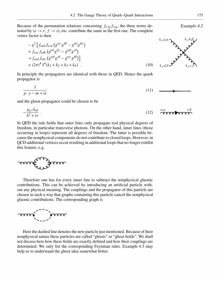
4.2 The Gauge Theory of Quark–Quark Interactions 175
Because of the permutation relations concerning fe fg frsg, the three terms de-noted by (e → r, f → s), etc. contribute the same as the first one. The completevertex factor is then
− g2 [ feab fecd(gαγ gβδ− gαδgβγ
)+ feac fedb
(gαδgβγ − gαβgγδ
)+ fead febc
(gαβgγδ− gαγ gβδ
)]× (2π)4 δ4(k1+ k2+ k3+ k4) . (10)
In principle the propagators are identical with those in QED. Hence the quarkpropagator is
1
p ·γ −m+ iε(11)
and the gluon propagator could be chosen to be
−gµνδab
k2+ iε. (12)
In QED the rule holds that outer lines only propagate real physical degrees offreedom, in particular transverse photons. On the other hand, inner lines (thoseoccurring in loops) represent all degrees of freedom. The latter is possible be-cause the nonphysical components do not contribute to closed loops. However, inQCD additional vertices occur resulting in additional loops that no longer exhibitthis feature, e.g.
Therefore one has for every inner line to subtract the nonphysical gluoniccontributions. This can be achieved by introducing an artificial particle with-out any physical meaning. The couplings and the propagator of this particle arechosen in such a way that graphs containing this particle cancel the nonphysicalgluonic contributions. The corresponding graph is
Here the dashed line denotes the new particle just mentioned. Because of theirnonphysical nature these particles are called “ghosts” or “ghost fields”. We shallnot discuss here how these fields are exactly defined and how their couplings aredetermined. We only list the corresponding Feynman rules. Example 4.3 mayhelp us to understand the ghost idea somewhat better.
Example 4.2
k ,a1 ,a1k ,b2 ,b
k ,d4 ,d k ,c3 ,g
a,m n,b

176 4. Gauge Theories and Quantum-Chromodynamics
Example 4.2 One should be aware of the “i” in the expression for the vertex. This differ-ent phase compared with (7) shows that certain cancellations of ghost and gluonloops are possible. In that way, if the expression (21) below is implemented twicein the above ghost-loop diagram, additional “i” results in a minus-sign, so thatthe ghost-loop amplitude
partly cancels the gluon-loop amplitude
The Feynman rules discussed above are summarized in (15)–(21). In orderto indicate the different possible gauges, the gluon propagator is given in itsmost general form, assuming ∂µAµ = 0 (transverse gauge). From QED we al-ready know the Landau gauge (λ= 1) and the transverse propagator (λ→ 0).In fact an arbitrary mixing of these two cases can also be chosen. Gauge invari-ance implies that in the evaluation of a physical process all λ-dependent termscancel each other or are equal to zero. Therefore λ can be arbitrarily chosen, i.e.different from λ= 1, λ→ 0:
m, ,a k
c q, b p,
−ig fabc pµ(2π)4 δ4(p− k−q) (13)
and
i j
δij
p2+ iε(14)
Note that all Feynman graphs are frequently multiplied by an additional factor ibecause the starting point of a perturbative expansion is really i
∫L(x) d4x and
not∫
L(x) d4x. However, this leads only to an unimportant overall phase.

4.2 The Gauge Theory of Quark–Quark Interactions 177
k
a,m b,n
−δab
[gµν
k2+ iε− (1−λ) kµkν
(k2+ iε)2
], (15)
δab
k2+ iε, (16)
δij
p/−m+ iε, (17)
k b, ,n
p i, ,g p j' , ,b
g
(1
2λb)
ji(γν)βγ (2π)
4 δ4(p′ + k− p) , (18)
ig frst
[(kτ1 − kτ2
)gσ + (
k2 − k3)gστ
+ (kσ3 − kσ1
)gτ
](2π)4 δ4(k1+ k2+ k3) , (19)
Example 4.2

178 4. Gauge Theories and Quantum-Chromodynamics
Example 4.2 a k, ,a 1 b k, ,b 2
d k, ,d 4c k, ,g 3
− g2[
feab fecd(gαγ gβδ− gαδgβγ
)+ feac fedb(gαδgβγ − gαβgγδ
)+ fead febc
(gαβgγδ− gαγ gβδ
)](2π)4 δ4(k1+ k2+ k3+ k4) , (20)
m , ,a k
c q, b p,
−ig fabc pµ(2π)4 δ4(p− k−q) . (21)
EXAMPLE
4.3 Fadeev–Popov Ghost Fields
To define the gluon propagator (see (15) of the last Example) properly one hasto specify a gauge. Otherwise the equation of motion (Maxwell equation) of thefree gluon field cannot be inverted to give the Green function of the field equa-tion. This problem is already familiar from Abelian theories as QED. If we writethe Lagrangian of the free photon field as
L=−1
4F2
=−1
2∂µAν(∂
µAν−∂νAµ)
= 1
2Aν
(gµν∂2−∂µ∂ν
)Aµ , (1)

4.2 The Gauge Theory of Quark–Quark Interactions 179
where a surface term is discarded after partial integration, the photon propaga-tor Dµν is the inverse of the sandwiched operator in (1)(
gµν∂2−∂µ∂ν)
Dνλ(x− y)= δµλ δ(x− y) . (2)
If we multiply (2) by the operator ∂µ, giving
(0 ·∂ν)Dνλ(x− y)= ∂λδ(x− y) , (3)
we see that Dµν is infinite. This is because the operator(gµν∂2−∂µ∂ν) has no
inverse. This is the projection operator onto tranverse modes. It is a general fea-ture of projection operators that they do not have an inverse, e.g. applied to anarbitrary function ∂µΛ it gives(
gµν∂2−∂µ∂ν)∂µΛ= (∂ν∂2−∂2∂ν)Λ= 0 . (4)
Indeed the operator has a zero eigenvalue and therefore cannot be inverted. Thephysical reason behind this is that one has to make sure to propagate only physi-cal degrees of freedom. All fields that are related only by gauge transformationsAµ→ Aµ+∂µΛ are propagated as well, which clearly gives an infinite contri-bution. This can be cured by fixing a particular gauge. To be definite we imposethe Lorentz condition
∂µAµ = 0 , (5)
which can be included in the Lagrangian in the general form
Lfix =− 1
2λ(∂µAµ)2
= 1
2λAµgµν∂
2 Aν , (6)
where λ is some arbitrary gauge parameter. Again a surface term has beenneglected. If we include the gauge fixing in (1), the arising operator is welldefined,
1
2Aµ
(gµν∂
2− (1−λ−1)∂µ∂ν
)Aν , (7)
and can be inverted to give the photon propagator in momentum space,
Dµν(k)=− 1
k2
(gµν− (1−λ)kµkν
k2
), (8)
where λ→ 1 corresponds to the Feynman and λ→ 0 to the Landau gauge. How-ever, in QED such a gauge-fixing term does not affect the general physics ofthe theory because the field χ = ∂µAµ, i.e. the longitudinal part of the pho-ton field does not interact with physical degrees of freedom. According to theAbelian Maxwell equation it obeys a free field equation ∂2χ = 0 and therefore
Example 4.3

180 4. Gauge Theories and Quantum-Chromodynamics
Example 4.3 does not mix with the transverse part of the photon field. The corresponding situ-ation for non-Abelian theories is much more complicated. For instance in QCDthe gauge-fixing field χa = ∂µAa
µ obeys the non-Abelian extension of the waveequation
∂2χa+ g f abc Ab µ∂µχc = 0 . (9)
Therefore the unphysical χ particles, i.e. the longitudinal part of the gluon field,can interact with the transverse (physical) components of Aa
µ. Those unphysicallongitudinal components contribute to gluon loops and therefore have to be sub-stracted. This substraction can be done by the introduction of unphysical ghostfields ηa that exactly cancel the χa fields. The introduction of the ηa fields ismost conviently done in the framework of path integral quantization6 and wasfirst done by De Witt, Fadeev, and Popov. In this framework it can be shown thatthe so-called Fadeev–Popov ghost fields obey the same equation (9) as the scalarχa fields, although they have to be quantized as fermion fields. Then, accordingto Fermi–Dirac statistics, each closed loop of ghost fields has to be accompaniedby a factor−1. For each gluon loop one has to include one ghost loop which can-cels exactly the longitudinal part of the gluons. The complete gauge-fixing termthen can be written as
L=Lfix+LF.P. (10)
with
LF.P. = ∂µηa †
(∂µηa+ g f abc Ab,µηc
)=−ηa †∂µDac
µ ηc , (11)
where again a surface term is neglected. From this Lagrangian one can derive theFeynman rules for the ghost propagators and ghost vertices.
EXAMPLE
4.4 The Running Coupling Constant
We discussed above that in general a perturbation series converges for a givencoupling constant only at some momentum transfers. This behavior is easilyunderstood, since the renormalized coupling constant is defined for a specificmomentum transfer. In QED, for example, one can choose the incoming andoutgoing photons to be on the mass shell, and then
e e
qm qm
6 See, e.g., W. Greiner and J. Reinhard: Field Quantization (Springer, Berlin, Heidel-berg, 1996).

4.2 The Gauge Theory of Quark–Quark Interactions 181
eR = e
[1− α
2πlog
(Λ2
m2
)] 12
for q2 = 0 . (1)
For other values of q2 this graph then yields a finite, q2-dependent renormaliza-tion, i.e., a finite additional contribution to every electromagnetic process. Thesecorrections can be given analytically and taken into account by a redefinition ofthe electric charge. We obtain in a massless QED 7
e2R
(q2)= e2
R
(q2 =−M2
)1−Ce2
R
(q2 =−M2
)ln(q2/−M2
) . (2)
The value of the constant C depends on the number of fermions consideredby the theory and on the fermion charges. From (2) it also follows that q2 = 0is a special value, quite unsuitable for renormalization (here eR is equal tozero). Therefore q2 =−M2 is usually chosen as the renormalization point.Equation (2) denotes the additional contributions to all massless QED graphscaused by vacuum polarization. e2
R(q2) is valid only for a certain q2 range: if
q2 < 0,Ce2R
(−M2)
ln(q2/−M2
)< 1. In this range it can be interpreted as
a physical charge. For q2 > 0, e2R(q
2) becomes formally complex and such aninterpretation is no longer possible. In the latter case e2
R(q2) reflects the fact that
the following graphs lead to different phases.
(3)
The divergence of this “charge” for
Ce2R
(−M2) ln
(q2
−M2
)→ 1
indicates the breakdown of perturbation theory. For values of −q2 this largethe contributions of two-loop corrections become as large as those of one-loopgraphs in (1), and so on. If the higher corrections are also taken into account, weobtain instead of (2) the nonconvergent expression
e2(q2)= e2(−M2)
1−Ce2(−M2) ln(
q2
−M2
)+C′e4(−M2) ln2
(q2
−M2
)+ . . .
. (4)
Since QCD is a scale-free theory, it is possible to define a running coupling con-stant for it, which takes the finite corrections due to the graphs shown in Fig. 4.7into account. We get
αs(q2)= αs(−M2)
1+ 11− 23 Nf(q2)
4π αs(−M2) ln(
q2
−M2
) , (5)
7 see W. Greiner and J. Reinhardt: Quantum Electrodynamics, 3rd ed. (Springer, Berlin,Heidelberg, 2003).
Example 4.4

182 4. Gauge Theories and Quantum-Chromodynamics
q q
q q
Fig. 4.7. QCD graphs takeninto account by αs(q2)
Fig. 4.8. Running couplingconstants for the unphysi-cal case of 6 and 12 dif-ferent massless quarks. Bothcurves assumeα(−100 GeV2)= 0.2
where Nf denotes the number of quark flavors with a mass much smaller than12
√−q2. We shall derive (5) in Sect. 4.4 after having introduced the necessarytechniques in Sect. 4.3. Here we only want to discuss its phenomenologicalmeaning. Equation (5) includes two parameters M2 and αs(M2), which, how-ever, are not independent of each other. It is possible to introduce a quantityΛ=Λ(M) such that
11− 23 Nf(q2)
4παs(−M2) ln(Λ2/M2)=−1 , (6)
leading to
αs(q2)= 4π
(11− 23 Nf(q2))ln(−q2/Λ2)
. (7)
Hence the running coupling constant is fixed for all momentum transfers byone parameter.Λ can be determined by investigating highly energetic e+e− pairannihilation and many other processes. The “world average” of these results is
αs(− (34 GeV)2
)≈ 0.14±0.02 . (8)
Clearly the q2 dependence of the strong coupling constant is determined by Nf ,i.e., the number of quarks with M2 < |q2|. In Fig. 4.8, (7) is plotted for Nf = 6

4.2 The Gauge Theory of Quark–Quark Interactions 183
Fig. 4.9. Charge screeningin QCD. Nf denotes thenumber of (massless) quarks
and Nf = 12.Λ has been fixed to obey (8). The plot for Nf = 6 increases rapidlyfor small values of
√−q2, i.e., the interaction can certainly not be described byperturbation theory below 500 MeV energy transfer. This conclusion is not validfor Nf = 12. Since at these energies the real physical hadrons have a stronglycorrelated structure rather than appearing as a group of free quarks, it follows im-mediately that the number of “light” quarks cannot be much greater than six. Infact only two “light”-quark doublets have been discovered. This example yields
αs(− (100 GeV)2
)= 0.2 ⇒ Λ= 112 MeV for Nf = 6 . (9)
The currently discussed values for the scale parameter of QCD, ΛQCD, rangefrom 100 MeV to 300 MeV. It should be mentioned that Fig. 4.8 contains an in-valid simplification. In contradiction to this figure, Nf decreases with decreasing√−q2, because an increasing number of quarks must be considered massive.
Equation (7) can be interpreted as antiscreening of the charge unlike the usualscreening in QED. The vacuum polarization graph in (1) leads in the case of QEDto a polarization of the vacuum, which in the context of field theory is a mediumwith well-defined, non-trivial features.8 This behavior is depicted in Fig. 4.10for an extended charge. In QCD the corresponding graph with a virtual quarkloop shows the same effect. Here, however, there is also a gluon contribution.Since the gluons carry a charge, their virtual excitations can also be polarized.Therefore the analogous graph in Fig. 4.9 is somewhat more complicated. Inparticular, the total charge distribution depends on the dominance of the quarkor gluon part. Although the latter is defined by the gauge group, the first partincreases with every additional quark until it dominates the theory and QCDshows the same behavior as QED. From this argument it also follows that theantiscreening in SU(N) gauge theories in principle increases with N . Even theexplicit form of that dependence can be understood. The gluon contribution issimply proportional to the number of possible permutations for the loop gluonsin Fig. 4.11.
8 see W. Greiner and J. Reinhardt: Quantum Electrodynamics, 3rd ed. (Springer, Berlin,Heidelberg, 2003)
Fig. 4.10. Charge screeningin QED
Fig. 4.11. Gluon vacuumpolarization for QCD

184 4. Gauge Theories and Quantum-Chromodynamics
Example 4.4
Fig. 4.12. Poles of theintegrand in (4.59) for
p0 <
√(p+k)2+m2
2. Inte-gration contours C1 and C2are those used in (4.60)
For QCD, i.e. SU(3), c can assume three values; for SU(N) there are cor-respondingly N values. Therefore (7) becomes, in the case of an SU(N) gaugetheory,
αN(q2)= 4π(
11× 13 N − 2
3 Nf)
ln(−q2/Λ2
N
) . (10)
4.3 Dimensional Regularization
Currently so-called dimensional regularization is considered to be the standardprocedure for regularizing quantum field theories. Only in special cases, wheresome specific disadvantages of this method show up, are other procedures, suchas Pauli–Villars regularization or the momentum-cutoff method, employed. Forlattice gauge theories, however, regularization is automatically provided by thelattice constant, which necessarily yields a rather special regularization scheme.In the following we discuss only dimensional regularization.
The basic observation that motivated dimensional regularization is that onlylogarithmic divergences in standard quantum field theories are encountered and

4.3 Dimensional Regularization 185
these vanish for any dimensionality smaller than 4. Thus if it is possible to definea generalized integration for noninteger dimensions “d” the usual divergenceswill show up as poles in “d−4” which should be relatively easy to isolate. Torealize this idea it is advisable first to simplify the divergences that occur bya trick known as “Wick rotation”, namely by continuing it to imaginary energies.As mentioned above, only logarithmic divergences are encountered, so a typicaldivergent integral has the form
i∫
d4k1
(k2−m21+ iε)
1[(p+ k)2−m2
2+ iε] . (4.59)
One awkward property of this integral is that its behavior for large kµ is not uni-form, since k2 = (k0)2− (k)2 can stay small even when k0 and |k| both becomelarge. This problem can be circumvented by continuing k0 to ik0
E (k→ kE ),implying that
k2 →−(k0E )
2− (kE )2 =−k2
E ,
with k2E = (k0
E )2+ (kE )
2. (kE )µ is obviously a Cartesian vector that becomesuniformly large if (kE )µ→∞, so it is much easier to analyze the ultravioletdivergences for (kE )µ than for kµ.
To perform the Wick rotation one has to deform the integration path of k0 inthe complex plane. Figures 4.12 and 4.13 show the positions of the poles. We
Fig. 4.13. Poles of theintegrand in (4.59) for
p0 >
√(p+k)2+m2
2. Inte-gration contours C1 and C2are those used in (4.60)

186 4. Gauge Theories and Quantum-Chromodynamics
now use
∞∫−∞
dk0 · · ·+−i∞∫+i∞
dk0 · · ·+∫C1
dk0 · · ·+∫C2
dk0 . . .
=⎧⎨⎩ 0 for Fig. 4.12
residue for k0 =√(p+k)2+m2
2− p0; for Fig. 4.13. (4.60)
The ε prescription in (4.59) guarantees that the integrals over the arcs at infinity,∫C1
dk0 and∫C2
dk0, vanish. This can easily be seen if we use
1
(k2−m21+ iε)
1
(p+ k)2−m22+ iε
=−i
∞∫0
dα eiα(k2−m21+iε)(−i)
∞∫0
dβ eiβ[(p+k)2−m2
2+iε]. (4.61)
From k0 = R eiϕ, 0 ≤ ϕ ≤ π2 , and π ≤ ϕ ≤ 3
2π with R →∞, we get
Im(k2)= R2 sin(2ϕ)+O(R) > 0 , (4.62)
such that all terms vanish exponentially. The result of the Wick rotation istherefore
i
∞∫−∞
d4k1
k2−m21+ iε
1
(p+ k)2−m22+ iε
=−∞∫
−∞d4kE
1
k2E +m2
1− iε
1
(pE + kE)2+m22− iε
+ possibly a finite residuum . (4.63)
The residuum that possibly appears is finite. As we intend to isolate and substractthe divergent part of the integral (4.59) we do not have to bother about this finitecontribution. We define the renormalized integral as (4.59) minus the divergentpart of (4.63). This definition is not affected by the finite residuum.
Next we proceed to define an abstract mathematical operation which we wantto call the d-dimensional integral:∫
ddkE f(kE ) .

4.3 Dimensional Regularization 187
First we impose the following conditions:
(1) Linearity∫ddkE[a f(kEµ)+bg(kEµ)]
= a∫
ddkE f(kEµ)+b∫
ddkE g(kEµ) . (4.64)
(2) Invariance of the integral under finite shifts (pµ finite)∫ddkE f(kEµ)=
∫ddkE f(kEµ+ pEµ) . (4.65)
(3) A scaling property∫ddkE f(λkEµ)= λ−d
∫ddkE f(kEµ) . (4.66)
From these definitions it is not clear what is meant by a Lorentz-vector kµ ind dimensions. The point is that it is always sufficient to treat scalar integrals.Any vectorlike integral is completely specified by its values if contracted withfew linearly independent vectors and those scalar integrals can be analyticallycontinued. Bearing this in mind it is, however, helpful to use vectors like kµ asa shorthand for a collection of suitably defined scalar products.
The d-dimensional integral is now defined by its action on a set of basisfunctions
λ(A, Pµ)= e−A(k+P)2 . (4.67)
Properties (4.64) and (4.65) guarantee that all functions decomposed in this basiscan be integrated once the integral∫
ddkE e−Ak2E (4.68)
is known. Here the scaling property (4.66) becomes important, since it reducesany such integral to a single one:∫
ddkE e−Ak2E = A−
d2
∫ddkE e−k2
E . (4.69)
As we want the d-dimensional integral to coincide with the usual one for integervalues of d we impose the condition∫
ddkE e−k2E = π
d2 . (4.70)

188 4. Gauge Theories and Quantum-Chromodynamics
This relation is verified for integer d in Exercise 4.5. We note for later use thatin Exercise 4.5, (8), we also derive
∞∫−∞
ddk e−k2 = 1
(d−2)!!
(2π)
d2 d even
2 (2π)d−1
2 d odd
∞∫0
dk kd−1e−k2. (4.71)
Now, for any function f(k) which can be expanded into Gaussians, i.e.
f(k)=∑
n
cn e−An(k+pn)2, (4.72)
one obtains
∞∫−∞
ddkE f(k2E)=
1
(d−2)!!
(2π)
d2 d even
2 (2π)d−1
2 d odd
×∞∫
0
dkE kd−1E f(k2
E) . (4.71b)
With Γ( 1
2
)=√π and the unifying relation
2(π)d2
Γ( d
2
) =⎧⎪⎪⎨⎪⎪⎩
d even : 2πd2 × 2
d−2 × 2d−4 ×· · ·× 2
2 = (2π)d2
(d−2)!!
d odd : 2πd2 × 2
d−2 × 2d−4 ×· · ·× 2
1 × 1√π= 2(2π)
d−12
(d−2)!!(4.73)
(4.71b) can be written as
∞∫−∞
ddkE f(k2E)=
2(π)d2
Γ(d
2
) ∞∫0
dkE kd−1E f(k2
E) . (4.71c)
This equation is most important and will be used constantly during dimensionalregularization.

4.3 Dimensional Regularization 189
EXERCISE
4.5 The d-Dimensional Gaussian Integral
Problem. Derive (4.65) for integer d.
Solution. Omitting the subscript “E” in this exercise, we define for integer dand Euclidian kµ, µ= 0, 1, 2, . . . , d−1,
k0 = k cosϑ1 ,
k1 = k sinϑ1 cosϑ2 ,
k2 = k sinϑ1 sinϑ2 cosϑ3 ,
...
kd−2 = k sinϑ1 sinϑ2 . . . sinϑd−2 cosϑd−1 ,
kd−1 = k sinϑ1 sinϑ2 . . . sinϑd−2 sinϑd−1 (1)
and calculate the Jacobian row by row
J = ∂(k0k1k2 . . . kd−1)
∂(k, ϑ1, ϑ2 . . . ϑd−1)
=
∣∣∣∣∣∣∣∣cosϑ1 −k sinϑ1 0 . . .
sinϑ1 cosϑ2 k cosϑ1 cosϑ2 −k sinϑ1 sinϑ2 . . .sinϑ1 sinϑ2 cosϑ3 k cosϑ1 sinϑ2 cosϑ3 k sinϑ1 cosϑ2 cosϑ3 . . .
......
.... . .
∣∣∣∣∣∣∣∣= kd−1 cosϑ1 cosϑ1(sinϑ1)
d−2+ sinϑ1 sinϑ1(sinϑ1)d−2
×∣∣∣∣∣∣
cosϑ2 − sinϑ2 . . .sinϑ2 cosϑ3 cosϑ2 cosϑ3 . . .
......
. . .
∣∣∣∣∣∣= . . .
= kd−1(sinϑ1)d−2(sinϑ2)
d−3 . . . (sinϑd−3)2
×∣∣∣∣∣ cosϑd−2 − sinϑd−2 0
sinϑd−2 cosϑd−1 cosϑd−2 cosϑd−1 − sinϑd−2 sinϑd−1sinϑd−2 sinϑd−1 cosϑd−2 sinϑd−1 sinϑd−2 cosϑd−1
∣∣∣∣∣= kd−1(sinϑ1)
d−2(sinϑ2)d−3 . . . (sinϑd−2)
×∣∣∣∣ cosϑd−1 − sinϑd−1
sinϑd−1 cosϑd−1
∣∣∣∣= kd−1(sinϑ1)
d−2(sinϑ2)d−3 . . . (sinϑd−2) . (2)

190 4. Gauge Theories and Quantum-Chromodynamics
Exercise 4.5 The Gaussian integral thus becomes
∞∫−∞
ddk e−k2(3)
=∞∫
0
dk kd−1 e−k2
π∫0
(sinϑ1)d−2 dϑ1 . . .
π∫0
sinϑd−2 dϑd−2
π∫0
dϑd−1 .
We use partial integration to get
π∫0
(sinϑ)n−1 sinϑ dϑ
=[(sinϑ)n−1(− cosϑ)
]π0− (n−1)
π∫0
(sinϑ)n−2 cosϑ(− cosϑ)dϑ
= (n−1)
π∫0
[(sinϑ)n−2− (sinϑ)n
]dϑ (4)
or
π∫0
(sinϑ)ndϑ = n−1
n
π∫0
(sinϑ)n−2dϑ .
For even n ≥ 2 we thus get
π∫0
(sinϑ)ndϑ = (n−1)!!n!!
π∫0
dϑ = (n−1)!!n!! π , (5)
and for n = 0 we have
π∫0
dϑ = π . (6)
For odd n we find
π∫0
(sinϑ)ndϑ = (n−1)!!n!!
π∫0
sinϑ dϑ
= (n−1)!!n!! ×2 . (7)

4.3 Dimensional Regularization 191
Inserting all these equations into (3) we get
∞∫−∞
ddk e−k2 =∞∫
0
dk kd−1e−k2Id
1
(d−2)!! ,
d even⇒ Id = (2π)d2 ,
d odd ⇒ Id = 2× (2π) d−12 . (8)
On the other hand, partial integration gives
∞∫0
dk kd−1 e−k2 = 1
2
∞∫0
dk kd−22k e−k2
= d−2
2
∞∫0
dk kd−3 e−k2
= (d−2)!!Kd , (9)
d even⇒ Kd =(
1
2
) d−22
∞∫0
dk ke−k2 =(
1
2
) d2
,
d odd ⇒ Kd =(
1
2
) d−12
∞∫0
dk e−k2 =(
1
2
) d−12√π
2. (10)
All together this gives
∞∫−∞
ddk e−k2 = 1
(d−2)!! (d−2)!! Id Kd = πd2 , (11)
which completes our proof.
With (4.67) all integrals can be expanded in a sum of Gaussians,
f(k)=∑
n
cn e−An(kE+pnE)2, (4.74)
and f(k) can now be integrated d-dimensionally, i.e.∫ddkE f(kE )=
∑n
cn A− d
2n π
d2 . (4.71d)
However, it is not clear whether this sum converges. If it does for some integerd, i.e., if the original integrand converges, then the expression (4.71d) also con-verges. This is not true for divergent integrals. In this case the d-dimensional
Exercise 4.5

192 4. Gauge Theories and Quantum-Chromodynamics
integral may still be finite. Thus all finite parts of the momentum integrals arereproduced. The infinite parts, associated, for example, with integrands like1/(k2
E)α or (k2
E)α, which we want to subtract, will lead to infinite nonconvergent
sums over Gaussians, the resulting term on the right-hand side of (4.71b). Thesewill be subtracted during renormalization. We will see below that these infiniteparts are different for d-dimensional integrals than for normal ones. Actuallymany divergences of usual integrals vanish automatically for d-dimensional in-tegrals, and the important points to keep in mind throughout this discussionare:
d-dimensional convergent integrals for d → n (where n is an integer) coincidewith the normal convergent n-dimensional integrals.
n-dimensional divergent integrals are in general different from the correspond-ing d → n limit of the d-dimensional integral. The latter is in general lessdivergent.
For example, for dimensional reasons the integral∫ddk
1(k2+m2
)µ (4.75)
behaves as (m2)d/2−µ. Thus for d = 4 we will encounter a logarithmic di-vergence for µ= 2, and a powerlike divergence for µ< 2 which has to beregularized by a cut-off in conventional n-dimensional integration. However, wewill show (see (4.81) below) that in dimensional regularization∫
ddk1(
k2+m2)µ ∼ Γ(µ−d/2) (m2)d/2−µ (4.76)
does pick up only logarithmic divergences even for µ< 2. For instance, forµ= 1 and d = 4+2ε one gets
Γ(1−2−ε)= Γ(−1−ε)= −Γ(−ε)1+ε =+(1−ε)
(1
ε+γE
)= 1
ε+γE−1+O(ε) (4.77)
which clearly is only a (dimensionless) logarithmic divergence.It is crucial to understand that our definition of a d-dimensional integral does
not always reduce to a normal integral in integer d dimensions. Instead it haspeculiar properties, for example,∫
ddkE
(k2
E
)ν = 0 for any ν , (4.78)
which follows directly from the scaling axiom (4.66). Indeed we have∞∫
−∞ddkE
(λ2k2
E
)ν = λ2ν
∞∫−∞
ddkE
(k2
E
)ν = λ−d
∞∫−∞
ddkE
(k2
E
)ν. (4.79)

4.3 Dimensional Regularization 193
Because this holds for any λ, ν, d, one is directly led to (4.78). Actually ν =−d/2is the only power for which (4.78) does not imply the vanishing of this inte-gral, but since we make critical use of the fact that our renormalized integralsare analytic functions of all variables involved, like ν in (4.78), we have also todefine∫
ddkE
(k2
E
)− d2 = 0 . (4.80)
This derivation of (4.78) is actually not without problems, because it assumesthat
∫ddkE (k2
E)ν exists, which is only true after a specific definition such as
limm2→0∫
ddkE (k2E +m2)ν. To be on the safe side it is better to regard (4.78) as
a definition that is made plausible by (4.65). A peculiar feature of (4.78) seems tobe that it leads to finite results even for theories for which arbitrarily high diver-gences occur. While this is formally true it is of no importance since such theoriescannot be renormalized. They would require an infinite number of renormaliza-tion constants and counterterms and thus cannot be formulated consistently. Asan example let us mention a scalar field theory with a φ6 coupling. This couplingleads to divergent graphs like
which is divergent(∼ ∫
d4k[1/k2(k+ p)2
])and must be renormalized, leading
to a counter term of the form
which is a φ8 interaction. Continuing this argument we find that the renormalizedtheory has infinitely many interaction terms of the general form
∑∞n=3 cnφ
2n , andno consistent theory can be formulated. Note that for a φ4 interaction

194 4. Gauge Theories and Quantum-Chromodynamics
the counterterm is again φ4. This is the reason why scalar theories up to φ4
terms in the Lagrangian are renormalizable. In fact only those theories can berenormalized that have at most logarithmic divergences, and thus integrals like∫
d4k(
k2)3
cannot occur. For renormalizable theories the differences between n-dimensionalintegrals and d-dimensional integrals (with the limit d → n) is thereforeirrelevant.
Equation (4.78) is essential for deriving the following basic formula:
Iν,µ =∫
ddkE
(k2
E
)ν(k2
E +M2)µ = π
d2
(M2
)ν−µ+ d2 Γ
(ν+ d
2
)Γ(µ−ν− d
2
)Γ(d
2
)Γ(µ)
,
(4.81)
which we shall prove next. Using (4.78) we can rewrite Iν,µ in the followingmanner:
Iν,µ =∫
ddkE
(k2
E
)ν(k2
E +M2)µ = M2ν−2µ+d
∫ddkE
(k2
E
)ν(k2
E +1)µ
= M2ν−2µ+d∫
ddkE
[ (k2
E
)ν(k2
E +1)µ −∑
n
(k2
E
)νncn
](4.82)
with arbitrary constant coefficients νn and cn . These coefficients are now chosensuch that they cancel all potential divergences, i.e., all high powers of k2. Theintegral is then convergent and we simply apply (4.71c):
Iν,µ = M2ν−2µ+d 2πd2
Γ(d
2
) ∞∫0
dk2E
2
(k2
E
) d2−1
[ (k2
E
)ν(k2
E +1)µ −∑
n
(k2
E
)νncn
].
(4.83)
The trick is now to derive by partial integration a recurrence relation for the Iν,µ:
Iν,µ =(ν+ d
2 −1)
µ−1Iν−1,µ−1+M2ν−2µ+d 2π
d2
Γ( d
2
) 1
2
×(
k2E
)ν+ d2−1
[(k2
E +1)1−µ
1−µ −∑
n
(k2
E
)νn+1−ν cn
νn +1
]∞0
.
(4.84)
The second term can obviously be absorbed into the cns. In other words, cn canbe chosen such that it vanishes. This leaves us with the relation
Iν,µ = ν+ d2 −1
µ−1Iν−1,µ−1 for all real ν, µ . (4.85)

4.3 Dimensional Regularization 195
In view of the relation Γ(z+1)= zΓ(z), which uniquely defines the gammafunction, (4.85) suggests (d is fixed) the following ansatz for Iν,µ :
Iν,µ = Γ(ν+ d
2
)Γ(µ)
K(ν−µ) (4.86)
with an arbitrary function K(ν−µ). To fix K(ν−µ) we use the fact that(k2
E
)ν(k2
E +1)µ = (
k2E
)ν(k2
E +1)µ [(
k2E +1
)− k2
E
], (4.87)
Iν,µ = Iν,µ−1− Iν+1,µ . (4.88)
Inserting (4.86) into (4.88) gives
Γ(ν+ d
2
)Γ(µ)
K(ν−µ)=[Γ(ν+ d
2
)Γ(µ−1)
− Γ(ν+ d
2 +1)
Γ(µ)
]K(ν−µ+1)
⇒ K(ν−µ)=[(µ−1)−
(ν+ d
2
)]K(ν−µ+1)
=(µ−ν−1− d
2
)K(ν−µ+1) (4.89)
⇒ K(ν−µ)= Γ
(µ−ν− d
2
)const , (4.90)
where we have again used that the relation Γ(x+1)= xΓ(x) defines the gammafunction uniquely, up to a constant. The remaining constant in∫
ddkE
(k2
E
)ν(k2
E +M2)µ = 2πd/2
Γ(d
2
)M2ν−2µ+d
Γ(µ−ν− d
2
)Γ(ν+ d
2
)Γ(µ)
const (4.91)
can easily be fixed. We choose ν = 1−d/2 and µ= 2. With (4.71c) we get, onthe one hand,
∞∫0
ddkE
(k2
E
)1−d/2(k2
E +M2)2 =
2πd/2
Γ(d
2
) ∞∫0
dk2E
2
1(k2
E +M2)2
= 2πd/2
Γ(d
2
) 1
2
[−1
k2E +M2
]∞0
= πd/2
Γ( d
2
) 1
M2 (4.92)
and from (4.91), on the other hand,
2πd/2
Γ(d
2
)M2−d−4+dΓ (2−1) Γ (1)
Γ(2)const = 2πd/2
Γ( d
2
) 1
M2 const . (4.93)

196 4. Gauge Theories and Quantum-Chromodynamics
Comparing both expressions we conclude that const = 1/2, or∫ddkE
(k2
E
)ν(k2
E +M2)µ = πd/2
Γ( d
2
)M2ν−2µ+d Γ(µ−ν− d
2
)Γ(ν+ d
2
)Γ(µ)
. (4.94)
This is an important formula, since any integral appearing in the calculations ofFeynman graphs can be brought into this form. The steps are:
(1) Introduce Feynman parameters according to1
aα11 aα2
2 . . . aαmm
= Γ(α1+α2 . . . αm)
Γ(α1)Γ(α2) . . . Γ(αm)
1∫0
dx1
x1∫0
dx2 . . .
xm−2∫0
dxm−1
× xα1−1m−1 (xm−2− xm−1)
α2−1 . . . (1− x1)αm−1
[a1xm−1+a2(xm−2− xm−1)+ . . .+am(1− x1)]α1+α2...αm. (4.95)
This relation will be derived in Exercise 4.7.
(2) Shift the momentum variable of the loop kµ such that the linear term in thedenominator vanishes:∫
ddkEf(kEµ)(
k2E +m2
)β . (4.96)
(3) Use the fact that all kµ have to be contracted with some other kλ according tokµkλ→ gµλk2/d. Otherwise the term vanishes if individual components kµ areinverted, kµ→−kµ. The resulting expressions are sums of terms of the form(4.94).
For convenience we give a list of expressions which shows the results from dif-ferent terms following steps 2 and 3. The integrals on the left-hand sides are inMinkowski space; therefore a factor “i” appears on the right, owing to the Wickrotation.∫
ddk1(
k2+2k · p+m2)α = iπd/2(
m2− p2)α−d/2
Γ (α−d/2)
Γ(α). (4.97)
∫ddk
kµ(k2+2k · p+m2
)α = iπd/2(m2− p2
)α−d/2
Γ (α−d/2)
Γ(α)(−pµ) . (4.98)
∫ddk
k2(k2+2k · p+m2
)α = iπd/2(m2− p2
)α−d/2
1
Γ(α)
[Γ
(α− d
2
)p2
+Γ(α−1− d
2
)d
2
(m2− p2
) ]. (4.99)

4.3 Dimensional Regularization 197
∫ddk
kµkν(k2+2k · p+m2
)α = iπd/2(m2− p2
)α−d/2
1
Γ(α)
[Γ
(α− d
2
)pµ pν
+Γ(α−1− d
2
)1
2gµν
(m2− p2
) ]. (4.100)
∫ddk
kµkνkλ(k2+2k · p+m2
)α = iπd/2(m2− p2
)α−d/2
1
Γ(α)
[−Γ
(α− d
2
)pµ pν pλ
−Γ(α−1− d
2
)(m2− p2
)× 1
2(gµν pλ+ gµλ pν+ gνλ pµ)
]. (4.101)
To check that (4.94) also reproduces (4.80) we use the following property of theΓ function:
Γ(β+1)= βΓ(β)
⇒ limβ→0
Γ(β)= limβ→0
1
βΓ(β+1)
= limβ→0
1
β
[1+βΓ ′(1)+O
(β2)]= 1
β+Γ ′(1) . (4.102)
This implies that
limµ→0
∫ddkE
(k2
E
)ν(k2
E +M2)µ
= limµ→0
πd/2
Γ( d
2
)M2ν+dΓ
(−ν− d
2
)Γ
(ν+ d
2
)µ= 0 . (4.103)
Equation (4.102) also allows us to write down in a uniform manner all the diver-gences that can occur on the right-hand side of (4.94). Such divergences occurif µ−ν−d/2 or ν+d/2 are negative integers or zero. The Γ function has nozeros on the positive real axes, so that 1/Γ(µ) does not create any divergences.With
limε→0
Γ(−n+ε)= limε→0
Γ(1−n+ε)−n+ε = lim
ε→0
Γ(2−n+ε)(−n+ε)(1−n+ε) = . . .
(4.104a)
all divergences can be related to limε→0 Γ(ε) from (4.94). Let us discuss as anexample
limε→0
Γ(−3+ε)= limε→0
Γ(ε)
(−3+ε)(−2+ε)(−1+ε)= lim
ε→0
(−1
6
)(1+ ε
3+ ε
2+ε
)(1
ε+Γ ′(1)
)= lim
ε→0
(−1
6ε
)− 1
6
(Γ ′(1)+ 1
3+ 1
2+1
)

198 4. Gauge Theories and Quantum-Chromodynamics
=−Γ′(1)+ 11
6
6− 1
6limε→0
1
ε. (4.104b)
All possible divergences (which can be only logarithmic for renormalizabletheories) are therefore proportional to 1/ε, and (4.94) and (4.104a,b) alreadydetermine dimensional regularization.
Dimensional regularization, i.e., the separation of the divergent and finiteparts, is realized by identifying the 1/ε terms with the divergent part and the rest,which is the finite one. The 1/ε terms are then absorbed into the renormalizationconstants, such as mass, charge, . . . , during renormalization.
To end this section, let us mention a second valuable formula for dimensionalregularization (d = 4+2ε):∫
ddxei p·x
(−x2)ν=−iπ2Γ(2−ν+ε)
Γ(ν)
(−4π2µ2
p2
)ε (−p2
4
)ν−2
, (4.105)
which allows us to perform d-dimensional Fourier transformations. It is derivedin Exercise 4.6.
EXERCISE
4.6 The d-Dimensional Fourier Transform
Problem. Derive the equation
∫ddx
ei p·x
(−x2)ν=−iπ2Γ(2−ν+ε)
Γ(ν)
(−4π2µ2
p2
)ε (−p2
4
)ν−2
. (1)
Solution. In three dimensions plane waves can be expanded into Bessel func-tions and Legendre polynomials according to
ei p·x = ei|p| |x| cos θ = . . . . (2)
To prove (1) we need the generalization of this expansion to arbitrary di-mensions. The exponential itself looks the same for any Euclidian dimension,namely
ei p·x = ei|p| |x| cos θ . (3)
Therefore the dimensionality enters only in the orthogonality property. The func-tions of θ that we call Ci(θ) shall be orthogonal with the weight (sin θ)d−2,because the d-dimensional volume element is proportional to (sinϑ)d−2 (see

4.3 Dimensional Regularization 199
Exercise 4.5, (2)):∫ddΩ Ci(cos θ)C j(cos θ)
∼π∫
0
dθ(sin θ)d−2 Ci(cos θ)C j(cos θ)
=1∫
−1
d cos θ (sin2 θ)(d−3)/2 Ci(cos θ)C j(cos θ)
=1∫
−1
dx (1− x2)(d−3)/2 Ci(x)C j(x) . (4)
Orthogonal polynomials with the weight (1− x2)d−1/2 are the “Gegenbauerpolynomials” C(α)
n (x).9 The important properties for us are
ei px cos θ = Γ(ν)( px
2
)−ν ∞∑k=0
(ν+ k) ik Jν+k(px)C(ν)k (cos θ) (5)
with arbitrary ν,
1∫−1
dx (1− x2)α−1/2 C(α)n (x)C(α)
n′ (x)
= δnn′π21−2αΓ(n+2α)
n! (n+α) [Γ(α)]2(α >−1
2
), (6)
and
C(α)0 (x)= 1 . (7)
From (6) and (7) we find that
1∫−1
dx (1− x2)α−1/2C(α)n (x)=
1∫−1
dx (1− x2)α−1/2C(α)n (x)C(α)
0 (x)
= δn0π21−2αΓ(2α)
α[Γ(α)]2
= δn0
1∫−1
dx (1− x2)α−1/2 . (8)
9 Their properties can be found, for example, in M. Abramowitz and A. Stegun: Hand-book of Mathematical Functions, Chap. 22. (Dover, 1972).
Exercise 4.6

200 4. Gauge Theories and Quantum-Chromodynamics
Exercise 4.6 Comparing (8) with the d-dimensional integral (4) we find thatα has to be chosenas α= d
2 −1. Using (6), relation (4) can now be denoted as∫ddΩ Cd/2−1
i (cos θ)Cd/2−1j (cos θ)= δij
π23−dΓ(i−2+d)
i! (i−1+ d2
) [Γ(d
2 −1)]2 ,
or ∫ddΩ Cα
i (cos θ)Cαj (cos θ)= δij
π21−2αΓ(i+2α)
i! (i+α) [Γ(α)]2 ,
(α= d
2−1
), (9)
and, furthermore,∫ddΩ =
1∫−1
dx (1− x2)(d−3)/2 = π23−dΓ(d−2)( d2 −1
) [Γ( d
2 −1)]2 . (10)
The angular integral is now easy to perform. We first substitute x0 →−ix0E to
go to Euclidian coordinates. We also substitute p0 → i p0E. Note that always the
time components only are Wick-rotated!∫ddx
ei p·x
(−x2)ν
=−i∫
ddxEei pExE cos θ
(x2E)ν
=−i
∞∫0
dxExd−1
E
(x2E)νΓ(α)
( pExE
2
)−α×
∞∑k=0
(α+ k)ik Jα+k(pExE)
∫ddΩ C(α)
k (cos θ)
=−i
∞∫0
dxE (xE)d−1−2νΓ(α)
( pExE
2
)−ααJα(pExE)
∫ddΩ
=−i2πd/2
Γ(d/2)Γ(d/2−1)
( pE
2
)1−d/2(
d
2−1
)
×∞∫
0
dxE (xE)d−1−2ν−d/2+1 Jd/2−1(pExE)
=−i2πd/2( pE
2
)1−d/2∞∫
0
dxE xd/2−2νE Jd/2−1(pExE)
=−i2πd/2( pE
2
)1−d/2(pE)
−1−d/2+2ν
∞∫0
dy yd/2−2ν Jd/2−1(y) . (11)

4.3 Dimensional Regularization 201
The remaining integral can be found in appropriate integral tables. 10
∞∫0
dy yd/2−2ν Jd/2−1(y)= 2d/2−2ν Γ(d
4 + d4 −ν
)Γ(d
4 − d4 +ν
) . (12)
Putting all this together we get∫ddx
ei p·x
(−x2)ν=−iπd/2(pE)
2ν−d 2d/2 2d/2−2ν Γ(d/2−ν)Γ(ν)
. (13)
Finally we insert again d = 4+2ε to obtain the result
∫ddx
ei p·x
(−x2)ν=−iπ2
(p2
E
4
)ν−2 (4π
p2E
)εΓ(2−ν+ε)
Γ(ν), (14)
which completes our proof. Note that p2E =−p2 !
EXERCISE
4.7 Feynman Parametrization
Problem. Prove the most general form of the Feynman parametrization,
n∏i=1
1
aAii
= Γ(A)∏ni=1 Γ(Ai)
1∫0
∏ni=1 dxi x Ai−1
i(∑ni=1 ai xi
)A δ
(1−
n∑i=1
xi
), (1)
with A =∑ni=1 Ai by means of mathematical induction. The ai (i = 1, 2, ..., n)
are arbitrary complex numbers.
Solution. To prove (1) we start with the simple formula
1
a ·b =1∫
0
dx
(ax−b(1− x))2, (2)
which is obtained by observing that
1
a ·b =1
b−a
(1
a− 1
b
)= 1
b−a
b∫a
dz
z2 . (3)
10 See, for example, I. Gradshtein and I. Ryshik: Tables of Series, Products and Inte-grals, No. 6.151.14 (Harri Deutsch, Frankfurt am Main 1981).
Exercise 4.6

202 4. Gauge Theories and Quantum-Chromodynamics
Exercise 4.7 Substituting z = ax+b(1− x) one obtains (2). Equation (2) can be furthergeneralized to arbitrary powers by taking derivatives
∂A
∂aA
∂B
∂bB (4)
on both sides so that
1
aA ·bB= Γ(A+ B)
Γ(A)Γ(B)
1∫0
dxx A−1(a− x)B−1
(ax+b(1− x))A+B
= Γ(A+ B)
Γ(A)Γ(B)
1∫0
dx dyx A−1 yB−1
(ax+by)A+Bδ(1− x− y) . (5)
Thus we have proven (1) for n = 2. Now we assume that the formula (1) holdsfor n and prove that it is also valid for n+1. Let us start with the expression
1
aAn+1n+1
n∏i=1
1
aAii
= Γ(A)∏ni=1 Γ(Ai)
1∫0
∏ni=1 dxi x Ai−1
i(∑ni=1 ai xi
)A δ
(1−
n∑i=1
xi
)1
aAn+1n+1
,
(6)
where we multiplied (1) on both sides by 1/aAn+1n+1 . Applying (5) we can rewrite
(6) to obtain
n∏i=1
1
aAii
= Γ(A)∏ni=1 Γ(Ai)
1∫0
n∏i=1
dxi xAi−1i δ
(1−
n∑i=1
xi
)Γ(A+ An+1)
Γ(A)Γ(An+1)
×1∫
0
dxn+1dyyA−1x An+1−1
n+1(y∑n
i=1 ai xi +an+1xn+1)A+An+1
δ (1− y− xn+1) .
(7)
Now we change variables xi = yxi (i = 1, 2, . . . n) in the above equation andperform the y integration. After replacing xi by xi we obtain
n+1∏i=1
1
aAii
= Γ(A+ An+1)∏n+1i=1 Γ(Ai)
1∫0
∏n+1i=1 dxi x
Ai−1i(∑n+1
i=1 ai xi
)A+An+1δ
(1−
n+1∑i=1
xi
). (8)
This completes the proof of (1).

4.4 The Renormalized Coupling Constant of QCD 203
4.4 The Renormalized Coupling Constant of QCD
We shall now use dimensional regularization to calculate the renormalized QCDcoupling constant to lowest order. The divergent graphs contributing to the renor-malization of gs belong to three classes, shown in Figs. 4.14, 4.15, and 4.16. Letus work them out one by one.
Graph (a1). We start with vacuum polarization, in particular with thefermion graph (a1) in Fig. 4.14. This graph is depicted in greater detail inFig. 4.17. One may wonder why the quantum numbers of the outgoing gluonk′, a′, µ′ are not identical with those of the ingoing gluon. Of course, this is themost general case. It will turn out that indeed a = a′ (see (4.119)) and k = k′(momentum conservation), but µ = µ′. Furthermore, in (4.133) and below, weshall see that only the sum of all four vacuum polarization graphs (a1)–(a4) isproportional to 1
k2 (kµkµ′ − gµµ′k2), i.e. the projector which ensures gauge in-
Fig. 4.14. The vacuum po-larization graphs of QCD
Fig. 4.15. The self energygraphs of QCD
Fig. 4.16. The vertex cor-rection graphs of QCD

204 4. Gauge Theories and Quantum-Chromodynamics
Fig. 4.17. The variables cho-sen for the quark loop con-tribution to vacuum polar-ization
variance. Using the QCD Feynman rules it is easy to write down the polarizationtensor:
Πa a′ (a1)µµ′ (k)=
NF∑i=1
g2∫
d4q
(2π)4
× tr
λa
2
λa′
2
q/+ k/+m
(q+ k)2−m2+ iηγµ
q/+m
q2−m2+ iηγµ′
. (4.106)
NF is the number of quark flavors in the theory, or more precisely the numberof quarks with m2 |k2|. The whole calculation can be carried through for ar-bitrary m2, but one finds that the contribution is suppressed for m2 > |k2|. NFtherefore counts only the light flavors and for simplicity we can set m = 0 in whatfollows whenever this does not lead to infrared divergencies. The trace over thecolor indices gives simply
tr
λa
2
λa′
2
= δa a′
1
2. (4.107)
As usual we introduce Feynman parameters
1
(q+ k)2−m2+ iη
1
q2−m2+ iη
=1∫
0
dz1
[q2+2kqz+ (k2−m2)z−m2(1− z)+ iη]2
=1∫
0
dz1
[(q+ kz)2+ k2z(1− z)−m2+ iη]2 . (4.108)
To get rid of the linear term in the denominator we substitute qµ→ q′µ= qµ− kµz:
Π(a1)µµ′ (k)= g2 NF
2
1∫0
dz
∞∫0
d4q
(2π)4tr[q/+ k/(1− z)]γµ[q/− k/z]γµ′
[q2+ k2z(1− z)−m2+ iη]2 , (4.109)
where we have dropped the color indices, i.e.Πabµν = δabΠµν. Here the term pro-
portional to m2 in the nominator has already been dropped. Next we take the traceand neglect all terms proportional to odd powers of q. They are zero as can beseen by substituting qν for −qν. For the same reason in intergrations over evenpowers of q only diagonal terms contribute:∫
d4q qµqν f(q2)= gµν× const = 1
4
∫d4q gµν q2 f(q2) . (4.110)

4.4 The Renormalized Coupling Constant of QCD 205
The left-hand side is a Lorentz tensor. After integrating over q the only possibleLorentz tensor is gµν. By contracting both sides with gµν we see that the factor1/4 is necessary to have the correct normalization (tr g = gµµ = 4). Therefore(4.109) becomes
Π(a1)µµ′ (k)= g2 NF
24
1∫0
dz
×∞∫
0
d4q
(2π)42qµqµ′ −q2gµµ′ − z(1− z)(2kµkµ′ − k2gµµ′)
[q2+ k2z(1− z)−m2+ iη]2
= 2g2 NF
1∫0
dz
×∞∫
0
d4q
(2π)4−1
2q2gµµ′ − z(1− z)(2kµkµ′ − k2gµµ′)
[q2+ k2z(1− z)−m2+ iη]2 . (4.111)
Now only q2 appears in the integrand, so it can safely be continued to Euclidianspace, qµ→ qµ = (iq0, q), and translated into a d-dimensional integral:
Π(a1)µµ′ (k)⇒ 2g2 NF
1∫0
dz
∞∫0
iddq
(2π)4µ4−d
12 q2gµµ′ − z(1− z)(2kµkµ′ − k2gµµ′)
[q2− k2z(1− z)+m2− iη]2 .
(4.112)
We have introduced a dimensional quantity µ to keep the total dimension of theexpression unchanged. The integration is four-dimensional, i.e.
∫d4 . . . . If this
is changed into∫
dd . . . with the same integrand, a factorµ4−d ensures the samedimension of the whole expression. With (4.81) it follows that
Π(a1)µµ′ (k)=
2ig2 NF
(2π)4
1∫0
dzπ
d2µ4−d
Γ(d
2
) [m2− k2z(1− z)− iη
] d2−2
× Γ(2− d
2
)Γ(d
2
)Γ(2)
[−z(1− z)](
2kµkµ′ − k2gµµ′)
+ 2ig2 NF
(2π)4gµµ′
2
1∫0
dzπ
d2µ4−d
Γ( d
2
) [m2− k2z(1− z)− iη
] d2−1
× Γ(1− d
2
)Γ(1+ d
2
)Γ(2)
. (4.113)

206 4. Gauge Theories and Quantum-Chromodynamics
The terms on the right-hand side are divergent. For d = 4−2ε the first isproportional to
Γ
(2− d
2
)= Γ(ε)= 1
ε+Γ ′(1)+O(ε) , (4.114)
while the second term is proportional to
Γ(1− d
2
)Γ(1+ d
2
)Γ(d
2
) = 4−2ε
2Γ(−1+ε)
= (2−ε) Γ(ε)
(−1+ε)= (2−ε)(−1−ε)
(1
ε+Γ ′(1)
)+O(ε)
=−2
ε−1−2Γ ′(1)+O(ε) . (4.115)
We thus have
Π(a1)µµ′ (k)=
2ig2 NF
(2π)4µ4−d π
d2
(1
ε+Γ ′(1)
)
×1∫
0
dz−z(1− z)
[m2− k2z(1− z)]ε(
2kµkµ′ − k2gµµ′)
− 2ig2 NF
(2π)4µ4−d π
d2
(2
ε+1+2Γ ′(1)
)
×1∫
0
dz [m2− k2z(1− z)]1−ε 1
2gµµ′ . (4.116)
It can now be seen that m2 can safely be neglected. For this purpose the integrandis expanded in m2/k2:[
m2− k2z(1− z)]−ε = (−k2)−ε(z(1− z))−ε
(1− m2
k2z(1− z)
)−ε= (−k2)−ε(z(1− z))−ε
×(
1+εm2
k2
1
z(1− z)+O
(m4
k4
)). (4.117)
The leading z integral can be performed easily,
1∫0
dz [z(1− z)]1−ε = Γ(2−ε)Γ(2−ε)Γ(4−ε) =
[1−εΓ ′(2)
]2
3!−2εΓ ′(4)
= 1
3! −ε
3Γ ′(2)+ ε
3Γ ′(4) , (4.118)
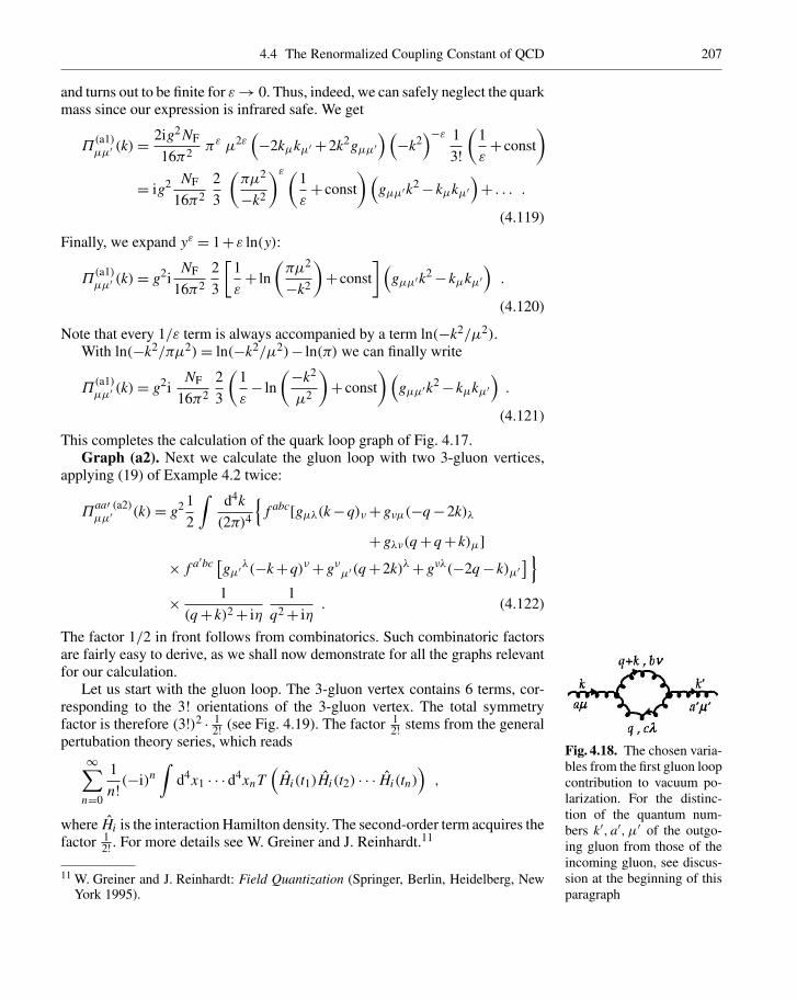
4.4 The Renormalized Coupling Constant of QCD 207
and turns out to be finite for ε→ 0. Thus, indeed, we can safely neglect the quarkmass since our expression is infrared safe. We get
Π(a1)µµ′ (k)=
2ig2 NF
16π2 πε µ2ε(−2kµkµ′ +2k2gµµ′
) (−k2
)−ε 1
3!(
1
ε+ const
)= ig2 NF
16π2
2
3
(πµ2
−k2
)ε (1
ε+ const
)(gµµ′k
2− kµkµ′)+ . . . .
(4.119)
Finally, we expand yε = 1+ε ln(y):
Π(a1)µµ′ (k)= g2i
NF
16π2
2
3
[1
ε+ ln
(πµ2
−k2
)+ const
] (gµµ′k
2− kµkµ′).
(4.120)
Note that every 1/ε term is always accompanied by a term ln(−k2/µ2).With ln(−k2/πµ2)= ln(−k2/µ2)− ln(π) we can finally write
Π(a1)µµ′ (k)= g2i
NF
16π2
2
3
(1
ε− ln
(−k2
µ2
)+ const
)(gµµ′k
2− kµkµ′).
(4.121)
This completes the calculation of the quark loop graph of Fig. 4.17.Graph (a2). Next we calculate the gluon loop with two 3-gluon vertices,
applying (19) of Example 4.2 twice:
Πaa′ (a2)µµ′ (k)= g2 1
2
∫d4k
(2π)4
f abc[gµλ(k−q)ν+ gνµ(−q−2k)λ
+ gλν(q+q+ k)µ]× f a′bc [gµ′λ(−k+q)ν+ gνµ′(q+2k)λ+ gνλ(−2q− k)µ′
] × 1
(q+ k)2+ iη
1
q2+ iη. (4.122)
The factor 1/2 in front follows from combinatorics. Such combinatoric factorsare fairly easy to derive, as we shall now demonstrate for all the graphs relevantfor our calculation.
Let us start with the gluon loop. The 3-gluon vertex contains 6 terms, cor-responding to the 3! orientations of the 3-gluon vertex. The total symmetryfactor is therefore (3!)2 · 1
2! (see Fig. 4.19). The factor 12! stems from the general
pertubation theory series, which reads∞∑
n=0
1
n!(−i)n∫
d4x1 · · · d4xnT(
Hi(t1)Hi(t2) · · · Hi(tn)),
where Hi is the interaction Hamilton density. The second-order term acquires thefactor 1
2! . For more details see W. Greiner and J. Reinhardt.11
11 W. Greiner and J. Reinhardt: Field Quantization (Springer, Berlin, Heidelberg, NewYork 1995).
Fig. 4.18. The chosen varia-bles from the first gluon loopcontribution to vacuum po-larization. For the distinc-tion of the quantum num-bers k′, a′, µ′ of the outgo-ing gluon from those of theincoming gluon, see discus-sion at the beginning of thisparagraph

208 4. Gauge Theories and Quantum-Chromodynamics
Fig. 4.19. The symmetryfactor for the graph in Fig.4.18. We get from the firstto the second line a factor of6 = 3 ·2 since we have threepossibilities to connect theleft external gluon line withone leg of the three gluonvertices. From the secondto the third line we aquirea factor of 3 due to the samereasoning. The connectionof the two remaining threegluon vertices again is pos-sible in two different ways.The factor 1/2! is due to thefact that we are consideringsecond order in perturbationtheory
Fig. 4.20. The symmetryfactor for the other graphs inFig. 4.14
Fig. 4.21. The symmetryfactor for the second graphin Fig. 4.15
As the two factors 62 = (3!)2 are absorbed in the 2×6 terms of the two3-gluon vertices we are left with a factor 1/2. The corresponding factors for theother graphs are derived in Fig. 4.20.
Following this scheme it is easy to obtain (see Figs. 4.20–4.24) any symmetry
factor of interest. The whole expression forΠaa′ (a2)µµ′ is obviously very similar to
(4.106) except for the different nominator, which we simplify first using
f abc f a′bc = δa a′C2 = δa a′ N for SU(N) . (4.123)
To obtain the symmetry factor for the second graph in Fig. 4.16 a generalremark will be helpful. To obtain symmetry factors for n-th order pertubationtheory we always have to deal with contributions like the one depicted below.Very schematically we displayed the n-th order contribution that can occur inQCD due to the 4 possible interaction vertices.
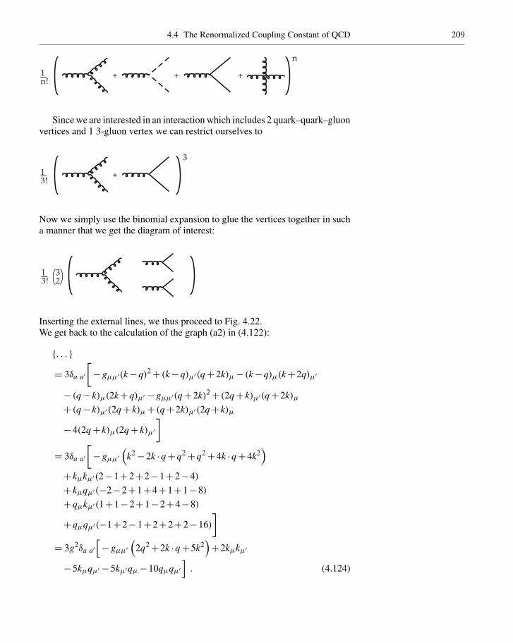
4.4 The Renormalized Coupling Constant of QCD 209
1n!
+ + +
n
Since we are interested in an interaction which includes 2 quark–quark–gluonvertices and 1 3-gluon vertex we can restrict ourselves to
13!
+
3
Now we simply use the binomial expansion to glue the vertices together in sucha manner that we get the diagram of interest:
13!
32
Inserting the external lines, we thus proceed to Fig. 4.22.We get back to the calculation of the graph (a2) in (4.122):
. . . = 3δa a′
[− gµµ′(k−q)2+ (k−q)µ′(q+2k)µ− (k−q)µ(k+2q)µ′
− (q− k)µ(2k+q)µ′ − gµµ′(q+2k)2+ (2q+ k)µ′(q+2k)µ+ (q− k)µ′(2q+ k)µ+ (q+2k)µ′(2q+ k)µ
−4(2q+ k)µ(2q+ k)µ′]
= 3δa a′[− gµµ′
(k2−2k ·q+q2+q2+4k ·q+4k2
)+ kµkµ′(2−1+2+2−1+2−4)
+ kµqµ′(−2−2+1+4+1+1−8)
+qµkµ′(1+1−2+1−2+4−8)
+qµqµ′(−1+2−1+2+2+2−16)
]= 3g2δa a′
[− gµµ′
(2q2+2k ·q+5k2
)+2kµkµ′
−5kµqµ′ −5kµ′qµ−10qµqµ′]. (4.124)

210 4. Gauge Theories and Quantum-Chromodynamics
Fig. 4.22. The symme-try factor for the secondgraph in Fig. 4.16 (3rd-orderperturbation theory implies1/3! binomial for the combi-nation of one 3-gluon vertexand two quark–gluon ver-tices:
(32
) = 3!2! 1! = 3)
Fig. 4.23. The symmetryfactor for the fourth graph inFig. 4.16
Fig. 4.24. The symmetryfactor for the third graph inFig. 4.16
We again substitute
qµ→ qµ− kµz (4.125)
and keep only the terms with even powers in qµ:
. . . ⇒ 3δa a′[−gµµ′
(2q2+2k2z2−2k2z+5k2
)+2kµkµ′ +5kµkµ′z+5kµkµ′z−10kµkµ′z
2−10qµqµ′]

4.4 The Renormalized Coupling Constant of QCD 211
⇒ 3δa a′[− gµµ′
(−2k2z(1− z)+5k2
)+2kµkµ′ +10kµkµ′z(1− z)−2gµµ′q
2− 5
2gµµ′q
2]
=: 3δa a′(
Aµµ′ + Bµµ′q2), (4.126)
defining Aµµ′ and Bµµ′ to abbreviate the corresponding terms. Repeating theFeynman trick (4.108) for the propagator product ((q+ k)2+ iη)−1 · (q2+ iη)−1
and introducing again Euclidean coordinates qµ = (iq0, q), the analogue to(4.112) now becomes
Πaa′ (a2)µµ′ (k)= 3
2g2δa a′ i
1∫0
dz
∞∫0
ddq
(2π)4µ4−d −Bµµ′ q2+ Aµµ′
[q2− k2z(1− z)− iη]2
= 3
2g2δa a′ i
1∫0
dzµ4−dπ
d2
(2π)41
ε
[Aµµ′ +2Bµµ′k
2z(1− z)]
×(−k2z(1− z)
)−ε+O(ε) . (4.127)
In the last step we have directly inserted the analogue expression from (4.119).The z integral now becomes
gµµ′(
2k2+ 9
2k22
) 1∫0
dz [z(1− z)]1−ε−5gµµ′k2
1∫0
dz [z(1− z)]−ε
+2kµkµ′
1∫0
dz [z(1− z)]−ε+10kµkµ′
1∫0
dz [z(1− z)]1−ε
= 11
6gµµ′k
2−5gµµ′k2+2kµkµ′ +10kµkµ′
1
6+O(ε)
=−19
6gµµ′k
2+ 22
6kµkµ′ +O(ε) , (4.128)
where we have used (4.118) and∫ 1
0 dz [z(1− z)]−ε = Γ(1−ε)Γ(1−ε)/Γ(2−2ε). This integral is a special case of the more general one12 B(x, y)=∫ 1
0 dzzx−1(1− z)y−1 = Γ(x)Γ(y)/Γ(x+ y). Thus, all together we get
Πaa′ (a2)µµ′ (k)= 3ig2δa a′
(16π)21
12
[1
ε− ln
(−k2
µ2
)+ const
](−19gµµ′k
2+22kµkµ′). (4.129)
12 See A.J.G. Hey and R.L. Kelly: Phys. Rep. 96, 72 (1983).

212 4. Gauge Theories and Quantum-Chromodynamics
k q,b+
ka ka'
m m '
q,c
Fig. 4.25. The chosen vari-ables for the ghost loop con-tribution to vacuum polar-ization. b and c describe thecolour of the ghosts
This expression is not gauge invariant ( kµΠ(a2)µµ′ = 0), which is quite reasonable,
since, as explained in Examples 4.2 and 4.3, gauge invariance is only restored byincluding the ghost terms. More precisely the ghost fields are constructed suchthat they cancel the contribution from the unphysical degrees of freedom of thegluon field. These unphysical degrees of freedom violate the gauge symmetry.
Graph (a3). To see how this happens we next calculate the ghost contribu-tion,
Πaa′ (a3)µµ′ (k)=−g2 f abc f a′cb
∫d4q
(2π)4qµ′(k+q)µ
[(q+ k)2+ iη](q2+ iη). (4.130)
Note that the color indices at f abc and f a′cb are constructed according to theorder: gluon, outgoing ghost, incoming ghost (see Example 4.2, (21)). The dif-ference in sign is due to the fact that the ghost fields anticommute. Using (4.123)and repeating the introduction of a Feynman parameter (see (4.108)) and shiftingaccording to qµ→ qµ− kµz, we obtain
Πaa′ (a3)µµ′ (k)= 3g2δa a′
1∫0
dz∫
d4q
(2π)4
14 gµµ′q2− kµkµ′z(1− z)(
q2+ k2z(1− z)+ iη)2 , (4.131)
where we also made use of qµ′qµ = 14 gµµ′q2 according to (4.110) and dropped
all terms linear in q in the nominator. After introducing Euclidean coordinatesand translating (4.130) into a d-dimensional integral (as was done in the step ofpassing from (4.111) to (4.112)), (4.130) becomes
Πaa′ (a3)µµ′ (k)= 3g2δa a′ i
16π2
(πµ2
−k2
)ε (1
ε+ const
)1∫
0
dz
(−2
4gµµ′k
2− kµkµ′)(1− z)z
= 3g2δa a′ i
16π2
[1
ε− ln
(−k2
µ2
)+ const
]1
12
(−gµµ′k
2−2kµkµ′). (4.132)
Together this gives
Πaa′ (a2)µµ′ (k)+Πaa′ (a3)
µµ′ (k)
= 3g2δa a′ i
16π2
[1
ε− ln
(−k2
µ2
)+ const
]20
12
(kµkµ′ − gµµ′k
2). (4.133)
The sum of the gluon-plus-ghost vacuum graph is thus again gauge invariant.This illustrates nicely the role of the ghost fields, namely to subtract out the un-physical components of the Aµ field, which are fixed by the chosen gauge. The

4.4 The Renormalized Coupling Constant of QCD 213
graph (a4) of Fig. 4.14 gives no contribution. This is best seen from the definingequation (4.78) for dimensional regularization:∫
ddq1
q2 = 0 .
The bubble is proportional to such a term because it does not depend on the ex-ternal momentum. The sum of all graphs shown in Fig. 4.14 is needed in therenormalization procedure following Fig. 4.29. We denote it here as
Π(a1)µν (k)+Π(a2)
µν (k)+Π(a3)µν (k)=
(kµkν− k2 gµν
)Za ,
where the divergent factor
Za = Z(a1)+ Z(a2)+ Z(a3) = g2
16π2
[1
ε− ln
(−k2
µ2
)][20
12C2− 2
3N f
]will be needed in the renormalization procedure following Fig. 4.29 below. Thefactor C2 will be discussed below, after (4.137).
Graph (b1). Next we calculate the self-energy graph
Σb(k)= g2∫
d4q
(2π)4γµ
q/
q2+ iηγµ
1
(q+ k)2+ iηtr
(λa
2
λa
2
)1
3. (4.134)
In this case we have to average over three quark colors, which leads tothe factor 1/3. Making use of γµq/γµ = γµqνγ νγµ = qνγµ(2gµν−γµγν)=2q/−γµγµq/= 2q/−4q/=−2q/, we have
Σb(k)= −2
34g2
∫d4q
(2π)4q/
[(q+ k)2+ iη][q2+ iη] . (4.135)
Following the same steps as before gives
Σb(k)=−8
3g2 i
16π2
(1
ε− ln
−k2
µ2 + const
)(−k/)
1∫0
dz z
= 4
3g2 i
16π2
(1
ε− ln
−k2
µ2 + const
)k/
≡ ik/Zb . (4.136)
The latter expression defines the divergent factor Zb, which will be important inthe renormalization procedure below (see Fig. 4.29 and (4.140)).
Graph (c1). We turn now to the vertex corrections Γ aµ ; see Fig. 4.27 and
(19) of Example 4.2. Γ aµ is defined as Λa
µ = γµλa/2+Γ a
µ (Γ aµ corrects the bare
vertex γµλa/2):
Γ a (c1)µ =−ig3
∫d4q
(2π)4f abc[gµλ(k−q)ν+ gνµ(−q−2k)λ+ gλν(2q+ k)µ
]× λb
2
λc
2
γνq/γλ
(q2+ iη)2[(q+ k)2+ iη
] . (4.137)
Fig. 4.26. The chosen vari-ables for the self-energygraph
Fig. 4.27. The chosen vari-ables for the first vertex cor-rection graph. The assign-ment of momenta k and 0for the outgoing quark linescorresponds to the specialLorentz system as explainedin the text

214 4. Gauge Theories and Quantum-Chromodynamics
Fig. 4.28. The chosen vari-ables for the second vertexcorrection graph
Here the quark propagator 1q/+m was taken in the limit m → 0, i.e. 1
q/+m → q/q2+iη
.
This, together with the one-gluon propagator 1q2+iη
, yields the above result.To make things easy we choose a very special kinematics: we choose the
outgoing quark to have zero momentum. Or, in other words, we calculate ina specific Lorentz frame where this is the case, relying on the fact that the diver-gencies and thus the renormalization constants for coupling constants, masses,and wave functions are Lorentz invariant. The divergent term is not affectedby this; only the finite ones are, and this makes things much easier. Using−i f abc λb
2λc
2 =− i2 f abc
[λb
2 ,λc
2
]= 1
2 f abc f dbc λd
2 = N δad2λd
2 ≡ C22λa
2 , where wehave utilized (4.123), we get
Γ a (c1)µ = 1
2C2λa
2g3
∫d4q
(2π)4
1∫0
dzΓ(3)
Γ(2)Γ(1)(1− z)
× (k/q/−q2)γµ−γµ(q2+2k/q/)−2q/(2q+ k)µ(q2+2qkz+ k2z+ iη)3
= 1
2C2λa
22g3
1∫0
dz (1− z)∫
d4q
(2π)4−2q2γµ−q2γµ+ . . .(q2+ k2z(1− z)+ iη)3
= iC2λa
2g3(+3)
1∫0
dz (1− z)µ4−d
16π2 γµπε(−k2z(1− z)
)−ε× Γ(3)Γ(ε)
Γ(2)Γ(3)+ . . .
= iC2λa
23g3 1
2
γµ
16π2
(1
ε− ln
−k2
µ2 + . . .). (4.138)
Graph (c3). Adopting again the same kinematics as for the calculation ofΓ
a (c1)µ (see Fig. 4.27), the second vertex graph Fig. 4.28 is
Γ a (c3)µ = g3
∫d4q
(2π)4λb
2γλλa
2(q/+ k/)γµq/
λb
2γλ
1
(q2+ iη)2((q+ k)2+ iη
)= g3
(4
3− 1
2C2
)λa
2(−2)
∫d4q
(2π)4
14(−2)γµq2
(q2+ iη)2((q+ k)2+ iη
)= g3
(4
3− C2
2
)iλa
2
γµ
16π2
(1
ε− ln
−k2
µ2 + . . .).
All third-order vertex correction graphs (C1) and (C2) together add up to
Γ a (c)µ = g3i
λa
2
γµ
16π2
(1
ε− ln
−k2
µ2 + . . .)(
−8
3+ 4
3+ 3
2C2− C2
2
)

4.4 The Renormalized Coupling Constant of QCD 215
= g3iλa
2
γµ
16π2
(1
ε− ln
−k2
µ2 + . . .)(
C2− 4
3
)≡ ig
λa
2γµZc . (4.139)
The divergent factor Zc defined in the last step will become important in therenormalization procedure below.
Now we can renormalize the coupling constant. The way in which the vari-ous contributions combine is shown in Fig. 4.29. The renormalization procedureis in fact rather easy. The square root of the vacuum polarization factor and theself-energy factor multiply each of the respective lines. Thus the quark–gluon
vertex acquires the factors(1+ Zb
) 12(1+ Zb
) 12 (1+ Zc)1 (1+ Za)
12 . Note, that
this convention differs from the one used in QED,13 where the renormalizationconstants Z are related to the one used here by Z = 1+ Z. Recall that we definedthe renormalization constants as (see (4.113), (4.116), (4.120))
Γ a(c)µ = ig
λa
2γµ Z(c) , Σ(b) = iγµkµ Zb , Π
(a)µµ′i(kµkµ′ −gµµ′) Za .
(4.140)
The renormalized quark–gluon vertex requires the full vertex correction Z(c),half of the correction to the gluon propagator and two times half of the correc-tions from the self-energy. Graphically we can depict that as follows:
The√(1+ Z) ·√(1+ Z) partiton of the Z factors over two vertices is illustrated
in Fig. 4.29 for quark–quark scattering with gluon exchange.The full quark–quark scattering amplitude with its various contributions up
to O(g60) is shown in Fig. 4.30.
13 See W. Greiner and J. Reinhardt: Quantum Electrodynamics, 2nd. ed. (Springer,Berlin, Heidelberg 1994).

216 4. Gauge Theories and Quantum-Chromodynamics
k q,b+
ka ka'
m m '
q,c
Fig. 4.29. The combinationof radiative corrections con-tributing to the renormaliza-tion of the coupling con-stant g
Adding all contributions, the total vertex is given by
Γ a(total)µ =−λ
a
2g0γµ
(1+ Zb
) 12(
1+ Zb) 1
2 (1+ Zc)1 (1+ Za) 1
2 (4.141)
=−iλa
2g0γµ
1− g2
16π2
[1
2
(20
12C2− 2
3NF
)−1
2×2× 4
3+ 4
3− C2
2+ 3
2C2
] [1
ε− ln
(−k2
µ2
)+ . . .
]=−i
λa
2g0γµ
1− g2
16π2
(22
12C2− 1
3NF
)[1
ε− ln
(−k2
µ2
)+ . . .
].
Fig. 4.30. Order g60 correc-
tions to the quark–quarkscattering amplitude
Here (1+ Za)12 ≈ (1+ (1/2)Za) has been approximated. The renormalized
coupling constant is obtained from (4.141) by subtracting the value of thecorrection at some renormalization scale M2:
gR = g0− g30
16π2
(11
6C2− 1
3NF
)[1
ε− ln
(−k2
µ2
)− 1
ε+ ln
(−M2
µ2
)]= g0+ g3
0
16π2
(11
6C2− 1
3NF
)ln
(−k2
M2
). (4.142)

4.4 The Renormalized Coupling Constant of QCD 217
An important quantity in QCD is the so-called β function, which will bediscussed below (see, e.g. Exercise 5.11) The β function is defined as β =M (∂gR/∂M)|−k2=M2 . It describes the dependence of the effective renormalizedcoupling on the renormalization scale M2. It can now be easily calculated:
β = M∂gR
∂M=− g3
0
16π2
(11
6C2− 1
3NF
)(2M
M2
)M
=− g30
16π2
(11
3C2− 2
3NF
)+O(g5
0) . (4.143)
This is the first term in the perturbative expansion for the β function. For QCDwe have to insert C2 = 3. Let us reflect on the β-function issue in order to under-stand the underlying ideas. Iteration and summation of the one-loop correctionsin terms of geometrical series leads to
g2(−k2)= g20
1+ g20
16π2
(113 C2− 2NF
3
)log
(−k2
M2
) (4.144)
where g0 is the coupling constant defined at the scale M2. This is the famousone-loop running coupling constant of QCD. Instead of doing this iteration andresumming the one-loop corrections, one may follow a more formal approach,as we will show now. As mentioned above, in QCD the so-called β functionallows a more general definition of the running coupling constant than just theresummation method, based on perturbation theory. The β function is defined assolution of the following differential equation
M
(∂g
∂M
)−k2=M2
≡ β(g)=−b0 g3+O(g5) (4.145)
and is determined order by order in perturbation theory. Above, in (4.143) and(4.144), we have determined the coefficient b0 entering on the right-hand side of(4.146) as
b0 = 1
16π2
(11
3C2− 2NF
3
). (4.146)
It is important to notice that (4.145) constitutes a differential equation for thecoupling constant g in its dependendce on the renormalization scale M, while(4.146) is based on a resummation of one-loop diagrams. There will be situationsin which the function β(g) can be determined nonperturbatively. Then (4.145)leads to more or less non perturbative expressions for the running coupling con-stant. This remark may demonstrate the advantage of the β-function method forthe calculation of g(−k2). We follow this idea and solve the differential equa-tion (4.145) to get an explicit solution for g(−k2) in the one-loop approximation.Separation of the variables g and M yields
g(−k2)∫g(M2)
dg
g3 =−b0
(−k2)2∫M2
dM
M(4.147)

218 4. Gauge Theories and Quantum-Chromodynamics
and therefore
1
g2(M2)− 1
g2(−k2)=−b0 ln
(−k2
M2
). (4.148)
Solving for g2(−k2)= 4παs(−k2) yields
αs(−k2)= αs(M2)
1+ αs4π
(11− 2NF
3
)ln(−k2
M2
) , (4.149)
which is the running coupling constant up to one-loop order (note that C2 = 3 inQCD).
It is instructive to compare our results (4.142) with those obtained fora different gauge, namely the Landau gauge, in which the gluon propagator is
−gµν+ kµkνk2
k2+ iη. (4.150)
In this gauge, instead of (4.133) one obtains
Π(a2)
µµ′ +Π(a3)
µµ′ |Landau = i3δaa′
16π2
[1
ε− ln
(−k2
µ2
)+ . . .
]× 26
12(kµkµ′ − gµµ′k
2) , (4.151)
instead of (4.136)
Σb(k)= 0 , (4.152)
and instead of (4.141)
Γ a (c)µ = i
λa
2
γµ
16π2
[1
ε− ln
(−k2
µ2
)+ . . .
]3
4C2 . (4.153)
Together this gives
gR = g0− g30
16π2
(13
12C2+ 3
4C2− 1
3NF
)[1
ε− ln
(−k2
µ2
)+ . . .
]= g0− g3
0
16π2
(11
6C2− 1
3NF
)[1
ε− ln
(−k2
µ2
)+ . . .
]. (4.154)
Thus the β function as an observable is gauge independent, as it must be, butthe renormalization of the wave function owing to the self-energy graph and thevacuum polarization graphs is gauge dependent. For completeness let us also cite

4.4 The Renormalized Coupling Constant of QCD 219
the result for the β function to third order:14
β(g)=− g30
(4π)2
(11
3C2− 3
2NF
)− g5
0
(4π)4
(34
3C2
2 −2C1 NF− 10
3C2 NF
)− g7
0
(4π)6
(2857
54C3
2 +C21 NF− 205
18C1C2 NF
−1415
54C2
2 NF+ 11
9C1 N2
F +79
54C2 N2
F
)(4.155)
with C2 = N (see (4.124)) for SU(N) and C1 = trλa
2λa
2 /N = 4/3 for quarks inthe fundamental representation.
For QCD this simplifies to
β(g)=− g3
(4π)2
(11− 2
3NF
)− g5
(4π)4
(102− 38
3NF
)− g7
(4π)6
(2857
2− 5033
18NF+ 325
54N2
F
). (4.156)
Up to second order this can be translated into an explicit solution for αs = g2R/4π
αs(µ)= 12π
(33−2NF) ln(µ2
Λ2
)⎡⎣1− 6(153−19NF)
(33−2NF)2
ln[ln(µ2
Λ2
)]ln(µ2
Λ2
)⎤⎦ ,
(4.157)
where we have introduced the famous ΛQCD parameter (see Example 4.3). It isexplained there thatΛQCD =ΛQCD
(M2
), i.e., it is a function of the renormaliza-
tion scale M2. To third order, such an explicit expansion cannot be given. This isbecause one actually expands simultaneously in lnµ2/Λ2 and ln
[ln(µ2/Λ2
)].
Such a double expansion becomes ambiguous at higher orders.Let us finally note that the higher terms of the β function, i.e., the cofficient of
g30 and g5
0 depend on the regularization scheme used, leading to different ΛQCDparameters for different renormalization schemes, which are correlated with dif-ferent expressions in the large bracket on the right-hand side of (4.157). This willbe explicitly discussed for the lattice gauge regularization in Sect. 7.1.
14 See O.V. Tarasov, A.A. Vladimirov, and A.Yu. Zharkov: Phys. Lett. B 93, 429 (1980);S.A. Larin and J.A.M. Vermaseren: Phys. Lett. B 303, 334 (1993).

220 4. Gauge Theories and Quantum-Chromodynamics
4.5 Extended Example: Anomalies in Gauge Theories
In this extended example we will discuss the origin of quantum anomalies. Let usfirst explain what the term quantum anomalies in field theory means. Considerthe action of a classical field theory which is invariant under certain symmetrytransformations. If this invariance cannot be preserved at the quantum level, i.e.,when quantum corrections are taken into account, such a phenomenon is calleda quantum anomaly.
We will concentrate on the physical meaning of the phenomenon and demon-strate the existence of two important anomalies in field theories: the chiral andthe scale anomaly.
4.5.1 The Schwinger Model on the Circle
Before discussing the scale anomaly in QCD and its connection to the QCDβ function we analyse the chiral anomaly in one of the simplest gauge fieldmodels, namely the Schwinger model on a circle. The Schwinger model is two-dimensional QED with massless Dirac fermions. The Langrange density for thismodel is
L=− 1
4e20
F2 + Ψ iγ ·DΨ , (4.158)
where e0 is the bare gauge coupling constant having mass dimension D = 2, F isthe gauge field strength tensor with components
Fµν = ∂µAν−∂νAµ , (4.159)
D denotes the covariant derivative with components
Dµ = ∂µ+ ie0 Aµ (4.160)
and Ψ is the two-component spinor field. The gamma matrices can be chosen asPauli matrices in the following way:
γ 0 = σ2 =(
0 −ii 0
), γ 1 = iσ1 =
(0 ii 0
), γ 5 = σ3 =
(1 00 −1
).
(4.161)
Note that γ 5 = γ 0γ 1. The Pauli matrices are in fact two dimensional represen-tations of the gamma matrices since
γµγν+γνγµ = 2 gµν with gµν = γ 5 µν . (4.162)
With the two dimensional antisymmetric tensor
ε =(
0 1−1 0
)(4.163)

4.5 Extended Example: Anomalies in Gauge Theories 221
one also verifies explicitely the relations
γµγν = εµνγ 5+ gµν , (4.164)
which will be useful later on.The spinorΨL ≡ (ψ1, 0)will be called left-handed (γ 5ΨL =+ΨL ), while the
spinor ΨR ≡ (0, ψ2) with γ 5ΨR =−ΨR will be called right-handed.In spite of the considerable simplifications compared to the four-dimensional
QED, the dynamics of the model (4.158) is still too complicated for our purpose.In order to simplify the situation further let us consider the system described by(4.158) in a finite spatial domain of length L . We impose periodic boundary con-ditions on the gauge field and (just for convenience) antiperiodic ones for themassless Dirac fermions. Thus
A
(t,−1
2L
)= A
(t,+1
2L
), Ψ
(t,−1
2L
)=−Ψ
(t,+1
2L
).
(4.165)
These conditions impose that the gauge field A and the Dirac fermions Ψcan be expanded in Fourier modes, i.e exp(ikx 2π/L) for the bosons andexp[i(k+1/2)x 2π/L) for the fermions.
Now let us recall that the Lagrange density (4.158) is invariant under the localgauge transformations
Ψ −→ eiα(t,x) Ψ, Aµ −→ Aµ−∂µα(t, x) . (4.166)
It is quite evident that all modes for the field A1 except for the zero mode can begauged away. Indeed, terms of the type a(t)exp(ikx 2π/L) in A1 with nonzeromomentum can be gauged away with α(t, x)=−(ik)−1a(t)exp(ikx 2π/L). Thischoice for the gauge function is in agreement with the boundary conditions(4.165), i.e. the gauge function is periodic on the circle with radius L . Asa consequence we can treat A1 in the most general case as x-independent.
However, the possibilities provided by gauge invariance are not exhaustedyet. There exist another class of legal gauge transformations which are notperiodic in x:
α(t, x)= 2π
Lnx n =±1,±2, . . . . (4.167)
Since ∂α/∂x = const. and ∂α/∂t = 0 the periodicitiy of the gauge field is not vio-lated. For the phase factor exp(iα) the analogous assertion is valid- the differenceof phases at the endpoints of the interval [−L/2, L/2] is equal to 2πn.
As a result, we arrive at the conclusion that A1 should not be considered in thewhole interval (−∞,+∞). The points A1, A1±2π/L , A1 =±4π/L , etc. areequivalent with respect to the gauge transformations (4.167) and must be iden-tified. In other words, the variable A1 should be considered only in the interval[0, 2π/L]. Beyond this interval we find gauge copies of this interval. In the com-monly accepted terminology we may say that A1 lives on the circle with length2π/L .

222 4. Gauge Theories and Quantum-Chromodynamics
So far we considered the µ= 1 component of the gauge field and this issufficient if we consider the gauge field as “external”. The µ= 0 componentof the gauge field is then responsible for the Coulomb interaction between thefermions. Since in two dimensions the Coulomb interaction grows linearly withthe distance between two fermions (confinement) the corresponding effect is ofthe order e0L at maximum. Now, if L is small, eoL 1, the Coulomb interactionnever becomes strong and we can neglect it in first approximation.
Let us turn to global symmetries of the model. The Lagrange density with fi-nite L is invariant under multiplication of the fermion field by a constant phase.According to the famous theorem of E. Noether one easily derives from thisa conserved current which turns out to be identical with the usual electromag-netic current:
Jµ = Ψ γµΨ , Q(t)= 0 , Q(t)=∫
dx j0(t, x) . (4.168)
The Lagrange density (4.158) admits another global symmetrie:
Ψ −→ eiαγ 5Ψ , (4.169)
which is called the global axial transformation. Again the theorem by Noetherensures the existence of a conserved current J5 µ, the so called axial current,which is conserved at the classical level just in the same way as the electro-magnetic current. Note that the axial transformation multiplies the left- andright-handed fermions by opposite phases. If the axial charge of the left-handedfermion is Q5 =+1, for the right-handed fermion Q5 =−1.
The conservation of Q and Q5 is equivalent to the conservation of the numberof the left-handed and right-handed fermions seperately. As we will see, in thequantized theory only the sum of chiral charges is conserved, so only one out ofthe two global symmetries of the classical theory survives the quantization of thetheory.
4.5.2 Dirac Sea
Let us now give a heuristic derivation of the chiral anomaly in the Schwingermodel on the circle before deducing it in a more rigorous manner.
In the two-dimensional electrodynamics the Dirac equation determining theenergy levels of the massless fermions is given by[
i∂
∂t+σ3
(i∂
∂x− A1
)]Ψ = 0 . (4.170)
For the kth stationary stateΨ ∼ exp(−iEkt) Ψk(x) and the energy of the kth stateis
EkΨk(x)=−σ3
(i∂
∂x− A1
)Ψk(x) . (4.171)

4.5 Extended Example: Anomalies in Gauge Theories 223
Furthermore, the eigenfunctions are proportional to
Ψk(x)∼ exp
[i
(k+ 1
2
)2π
Lx
], k = 0,±1,±2, . . . . (4.172)
As a result, we conclude that the energy of the kth level for the left-handedfermions is
Ek L =(
k+ 1
2
)2π
L+ A1 , (4.173a)
while for the right-handed fermions
Ek R =−(
k+ 1
2
)2π
L− A1 . (4.173b)
At A1 = 0, the energy levels for the left- and right-handed fermions are degener-ate. If A1 increases, the degeneracy is lifted and the levels are split. At the pointA1 = 2π/L the structure of the energy levels is precisely the same as for A1 = 0– the degeneracy takes place again. This is the remnant of the gauge invarianceof the original theory. It is important to note that the identity of the points A1 = 0and A1 = 2π/L is achieved in a non-trivial way. Since in passing from A1 = 0 toA1 = 2π/L a restructuring of the fermion levels take place. All left-handed lev-els are shifted upwards by one interval, while all right-handed levels are shifteddownwards by the same one interval, as shown in Fig. 4.31. This phenomenonlies on the basis of the chiral anomaly in the model at hand, as will become clearshortly.
Let us now proceed to field theory. The first task is the construction of theground state. To this end, following the well-known Dirac-prescription we fillup all levels lying in the Dirac sea, leaving all positive-energy levels empty.We will use
∣∣1L,R, k⟩
for the filled and∣∣0L,R, k
⟩for the empty energy levels
Fig. 4.31. Energy levels forright- and left-handed parti-cles as function of the fieldA1. The open circles showsthe right-handed hole beingshifted down to negative en-ergies, the full circle showsthe opposite behavior of afilled negative energy left-handed state moved to posi-tive energies with increasingfield

224 4. Gauge Theories and Quantum-Chromodynamics
with a given k. The subscript L (R) indicates that we deal with left-handed(right-handed) fermions.
At first, the value of A1 is fixed in the vicintiy of zero. Then, the fermionground state, as seen from the figure, reduces to
| Ψferm. vac.⟩ =
⎛⎝ ⊗k=−1,−2,...
∣∣1L , k〉⎞⎠ ⊗
⎛⎝ ⊗k=1,2,...
∣∣0L , k〉⎞⎠ ⊗
⎛⎝ ⊗k=0,1,2,...
∣∣1R, k〉⎞⎠ ⊗
⎛⎝ ⊗k=−1,−2,...
∣∣0R, k〉⎞⎠ .(4.174)
The Dirac sea, or all negative-energy levels are completely filled. Now let A1increase (adiabatically) from 0 to 2π/L . At A1 = 2π/L the fermion ground state(4.174) describes that state which, from the point of view of the normally filledDirac sea, contains one left-handed particle and one right-handed hole.
The interesting question is whether the quantum numbers of the fermionschange in the transition process from A1 = 0 to A1 = 2π/L . Naively we wouldsay that the appearance of the particle and the hole does not change the electriccharge. In other words, the electromagnetic current is conserved. On the otherhand, the axial charges of the left handed particle and the right-handed hole arethe same (Q5 = 1) and, hence, in the transition at hand
∆Q5 = 2 . (4.175)
Equation (4.175) can be rewritten as ∆Q5 = (L/π) ∆A1. Dividing by thetransition time we get
Q5 = L
πA1 , (4.176)
which implies, in turn, that the conserved charge is given by
Q5 =∫
dx
(J5 0− 1
πA1
). (4.177)
The conserved current corresponding to this charge is
J5 µ = J5 µ− 1
πεµνAν , ∂ · J5 = 0 , ∂ · J5 = 1
πεµν∂µAν , (4.178)
where ε01 =−ε10 =−ε01 = 1. The third equality in (4.178) is the famous axialanomaly in the Schwinger model. We succeeded in deriving it by “hand-waving”arguments by inspecting the picture of motion of the fermion levels in the ex-ternal field A1(t). It turns out that in this language the axial (or chiral) anomalypresents a widely known phenomenon: the crossing of the zero point in the en-ergy scale by a group of levels. The presence of the infinite number of levels andthe Dirac picture, according to which the emergence of a filled level from thesea means the appearance of a particle while the submergence of an empty level

4.5 Extended Example: Anomalies in Gauge Theories 225
into the sea is equivalent to the production of a hole, are the most essential elem-ents of the whole construction.15 With a finite number of levels there can be noanomaly.
4.5.3 Ultraviolet Regularization
In spite of the transparent character of this heuristic derivation almost all ofthe “evident” arguments above can be questioned by the careful reader. Indeed,why is the fermion ground state (4.174) the appropriate choice? In what sense isthe energy of this state minimal, taking into account the fact that, according to(4.173a) and (4.173b)
E ∼−∞∑
k=0
(k+ 1
2
)2π
L, (4.179)
and the series is divergent?The ground state (4.174) describing the fermion sector at A1 = 0 contains, in
particular, the direct product of an infinite large number of filled states with nega-tive energy. It is clear that the infinite product is ill-defined, and one cannot dowithout regularization in calculating physical quantities. The contribution fromlarge momenta should be somehow cut off.
In order to preserve the gauge invariance, it is possible and convenient to usethe regularization called the Schwinger- or ε-splitting. The regularization willprovide a more solid basis to the heuristic derivation presented above. Instead ofthe original currents
Jµ(t, x)= Ψ (t, x) γµ Ψ(t, x) , J5 µ(t, x)= Ψ (t, x) γµγ5 Ψ(t, x) , (4.180)
we introduce the regularized objects
J regµ (t, x)= Ψ (t, x+ε) γµ Ψ(t, x) exp
⎛⎝−i
x+ε∫x
dx A1
⎞⎠ ,
J reg5 µ(t, x)= Ψ (t, x+ε) γµγ5 Ψ(t, x) exp
⎛⎝−i
x+ε∫x
dx A1
⎞⎠ . (4.181)
In the calculation of physical quantities the limit ε−→ 0 is always implied. Atthe intermediate stages, however, all computations are performed with fixed ε.
15 Note the similarity of this effect to the diving of an empty electron state into the lowercontinuum in the presence of a supercritical external electric field. The hole in thelower continuum is subsequently emitted as a so-called spontaneous positron (for fur-ther details of the supercritical change of the neutral vacuum into a charged vacuumdue to Coulomb fields by spontaneous positron emission, see W. Greiner, B. Müller, J.Rafelski: Quantum Electrodynamics of Strong Fields, (Springer, Berlin, Heidelberg,1985), pp 122.

226 4. Gauge Theories and Quantum-Chromodynamics
The exponential factor in (4.181) ensures gauge invariance of the non-local(“split”) currents. Without this exponential any composite operator like theelectromagnetic current or the axial current transforms under the local phasetransformations (4.165) like
Ψ †α(t, x+ε) Ψβ(t, x)
−→ exp [−iα(x+ε)+ iα(x)] Ψ †α(t, x+ε) Ψβ(t, x) . (4.182)
The gauge transformation of A1 (A1 −→ A1−∂α(x)/∂x) compensates for thephase factor in (4.182).
Now, there is no difficulty to calculate the electric and axial charges of thestate (4.174). If
Q(t)=∫
dx J reg0 (t, x) , Q5(t)=
∫dx J reg
5 0 (t, x) , (4.183)
then we get for the fermion ground state
Q = QL +Q R , Q5 = QL −Q R , (4.184)
QL =−∞∑
k=−1
exp (−iε Ek L)
=−∞∑
k=−1
exp
−iε
[(k+ 1
2
)2π
L+ A1
], (4.185)
Q R =+∞∑k=0
exp (+iε Ek R)
=+∞∑k=0
exp
−iε
[(k+ 1
2
)2π
L+ A1
]. (4.186)
In the limit ε−→ 0 both charges, QL and Q R, turn into the sum of units – eachunit represents one filled level from the Dirac sea. Performing the summation
QL = e−iε A1
1− e+iε 2π/L, (4.187)
Q R = e−iε A1
1− e−iε 2π/L(4.188)
and expanding in ε we arrive at
QL = L
−iε2π+ L
2πA1+O(ε) , (4.189)
Q R = L
+iε2π− L
2πA1+O(ε) (4.190)
for the fermion ground state (4.174).

4.5 Extended Example: Anomalies in Gauge Theories 227
Equations (4.189) show that under our choice of the fermion ground statethe charge of the vacuum vanishes, Q = QL +Q R = 0. There is no time depen-dence – the charge is conserved. The axial charge consists of two terms: the firstrepresents an infinitely large constant and the second one gives a linear A1 de-pendence. In the transition from A1 = 0 to A1 = 2π/L the axial charge changesby two units.
These conclusions are not new for us. We have found just the same from theillustrative picture described above in which the electric and axial charges of theDirac sea are determined intuitively. Now we learned how to sum up the infiniteseries of units, i.e. the charges of the “left-handed” and “right-handed” seas.
It is very important to note, that there is no regularization ensuring simulta-neously the gauge invariance and conservation of the axial current.
Now, we leave the issue of charges and proceed to the calculation of thefermion-sea energy, the problem which could not be solved at the naive level,without regularization. Fortunately, all necessary elements are already prepared.The fermion part of the Hamiltonian
H =−Ψ †(t, x) σ3
(i∂
∂x− A1
)Ψ(t, x) (4.191)
reduces after the ε-splitting to
Hreg =−Ψ †(t, x+ε) σ3
(i∂
∂x− A1
)Ψ(t, x) exp
⎛⎝−i
x+ε∫x
dx A1
⎞⎠ .
(4.192)
This formula implies the following regularized expressions for the energy of the“left-handed” and “right-handed” seas:
EL =−∞∑
k=−1
Ek L exp (−iε Ek L) , (4.193a)
ER =+∞∑k=0
Ek R exp (+iε Ek R) , (4.193b)
where the energies of the individual levels Ek L,R are given in (4.173a) and(4.173b) and the summation runs over all levels with negative energy. The ex-pressions (4.193a) and (4.193b) have the following meaning: in the limit ε−→ 0they reduce to the sum of the energies of all filled fermion levels from the Diracsea. Notice, that EL and ER can be obtained by differentiating the expressions(4.185) and (4.186) for QL,R with respect to ε:
EL =+i∂
∂εQL =+i
∂
∂ε
e−iε A1
1− e+iε 2π/L, (4.194a)
ER =−i∂
∂εQ R =−i
∂
∂ε
e−iε A1
1− e−iε 2π/L, (4.194b)

228 4. Gauge Theories and Quantum-Chromodynamics
where we have used (4.187) and (4.188). The total energy of the sea is then
Esea ≡ EL + ER
= e−iε A1
1− cos(2πε/L)
(2π
L+ i A1sin
(2π
Lε
)). (4.195)
Expanding in ε we get
Esea = (1− iε A1+ε2 A21+ . . . )
1−1+ 12
(2πL ε
)2+ . . .
(2π
L+ i A1sin
(2π
Lε
)+ . . .
)= L
2πA2
1+O(ε)+ a constant independent of A1 . (4.196)
One remark is in order here. From the very beginning we assumed that the dy-namics of A1 is negligible when compared to the dynamics of the fermions. Letus verify that this is indeed justified.
The effective Lagrange density determinig the quantum mechanics of A1 is
L= L
2e20
A21−
L
2πA2
1 . (4.197)
This is the ordinary harmonic oscillator with the wave function
L
e0π32
exp
(− L A2
1
2e0π12
)(4.198)
of the ground state and the level splitting
ωA = e0
π12
. (4.199)
The characteristic frequencies in the fermion sector are ωΨ ∼ L−1. Hence,ωA/ωΨ ∼ Le0 1.
4.5.4 Standard Derivation
It will be extremely useful to discuss the connection between the picture pre-sented above and the more standard derivation of the chiral anomaly in theSchwinger model. The following discussion will serve as a bridge between thephysical picture described above and the standard approach to anomalies in QCDand other gauge theories.
We would like to demonstrate that
∂ · J5 = 1
2πεµνFµν , (4.200)
by considering directly the the divergence of the axial current. Then we need tobother only about the ultraviolet regularization. In particular, the theory can beconsidered in the infinite space since the finiteness of L does not affect the resultstemming from the short distances.

4.5 Extended Example: Anomalies in Gauge Theories 229
One of the convenient methods of the ultrviolet regularization is due to Pauliand Villars. In the model at hand it reduces to the following: In addition to theoriginal massless fermions in the Lagrange density, heavy regulator fermionsare introduced with mass M0 whereas the limit M0 −→∞ is implied. Further-more, each loop of the regulator fermions is supplied by an extra minus signrelatively to the normal fermion loop. The role of the regulator fermions inthe low-energy regime (E M0) is the introduction of an ultraviolett cut-offin the formally divergent integrals corresponding to the fermion loops. Sucha regularization procedure automatically guarantees the gauge invariance and theelectromagnetic current conservation.
In the model regularized according to Pauli and Villars the axial current hasthe form
J5 µ = Ψ γµγ 5 Ψ + R γµγ 5 R , (4.201)
where R is the regulator fermion. In calculating the divergence of the regularizedcurrent the naive equations of motions can be used. Then,
∂ · J5 = Ψ(←∂ ·γγ 5+ →
∂ ·γγ 5)Ψ + R
(←∂ ·γγ 5+ →
∂ ·γγ 5)
R
= Ψ(
igγ · A1γ5+ igγ 5γ · A1
)Ψ
+ R(
igγ · A1γ5+ igγ 5γ · A1+2iM0
)R
= 2iM0 R γ 5 R . (4.202)
The divergence is non-vanishing, i.e. the axial current is not conserved! But, aswas expected, ∂µ J5 µ contains only the regulator anomalous term.
The next step is to contract the regulator fields and calculate the relevant dia-grams. In this context we may learn a new technique, the so-called backgroundfield technique which we shall use here in order to calculate the right hand sideof (4.202). One can write in momentum representation
2iM0 R γ 5 R =−2M0 trγ 5
γ ·P −M0
≡−2M0
∫d2 p
(2π)2trL+C
⟨p
∣∣∣∣∣ γ 5
γ ·P −M0
∣∣∣∣∣ p
⟩, (4.203)
where P = iD and trL+C means the trace with respect to spin (Lorentz) andcolour indices; |p〉 denotes a state vector describing a fermion with momen-tum p. Note, that we have taken into account the fact that the minus sign in thefermion loop does not appear for the regulator fermions.
Moreover,
1
γ ·P −M0= γ ·P +M0
γ ·Pγ ·P −M20
= γ ·P +M0
P 2+ 12 iεµνFµνγ 5−M2
0
. (4.204)

230 4. Gauge Theories and Quantum-Chromodynamics
The second equality here stems from the definition of the gamma matrices andthe following property[
Pµ,Pν
]=− [Dµ, Dν
]= i Fµν . (4.205)
In fact, using (4.162) and (4.164) one may verify
γ ·Pγ ·P = γµγν PµPν = 1
2
(γµγν
[Pµ,Pν
]+2gµν PµPν
)=P 2+ 1
2iγµγν Fµν =P 2+ 1
2iεµνγ 5 Fµν . (4.206)
Now, since M0 −→∞ the trace in (4.203) can be expanded in inverse powers ofM0. In this way we get
trγ 5
γ ·P −M0= tr
[γ 5 (γ ·P +M0) (4.207)
×(
1
P 2−M20
+ 1
P 2−M20
(−)1
2iεµνFµνγ
5 1
P 2−M20
+ . . .)]
.
The first term in the expansion vanishes after taking the trace of the gamma ma-trices. The third and all other terms are irrelevant because they vanish in the limitM0 −→∞. The only relevant term is the second one, where we can substituethe operator P = iD = i∂− A by the momentum p since the result is explicitlyproportional to the back ground field. Then
2iM0 Rγ 5 R =−2iM20
∫d2 p
(2π)21(
p2−M20
)2 εµνFµν . (4.208)
The integration over p can be done with the help of the Feynman integral
I0 ≡∫
dn p
(2π)n1
(p2−M20)α= i
(−π) n2
(2π)nΓ(α− n
2
)α
1
(−M20)α− n
2. (4.209)
Thus,
2iM0 Rγ 5 R = 1
2πεµνFµν . (4.210)
This computation completes the standard derivation of the anomaly. One shouldhave a very rich imagination to be able to see in these manipulaions the simplephysical nature of the phenomenon which has been described above (restruc-turing of the Dirac sea and level crossing). Nevertheless, this is the samephenomenon viewed from a different perspective – less transparent but moreeconomic since we get the final result very quickly using the well-developedmachinery of the diagram technique.

4.5 Extended Example: Anomalies in Gauge Theories 231
4.5.5 Anomalies in QCD
Before proceeding to quantum anomalies in QCD let us first list the symme-tries of the classical action. We will assume that the theory contains n f masslessquarks and for the moment forget the heavy quarks which are inessential in thegiven context. The correction due to small u-, d-, and s-quark masses can beconsidered seperately if necessary.
In the chiral limit, i.e. mq = 0, the classical Lagrange density is
L=n f∑q
(qa
Lαi(γ)αβ · (D)abqbLβ+ qa
Rαi(γ)αβ · (D)abqbRβ
)− 1
4Gaµν Gµν
a ,
qL,R = 1
2(1±γ5) q , (4.211)
where q is the quark field and G is the gluon field strength tensor. The action ofthe classical theory is invariant under the following global transformations:
(1) Rotation of fermions of different flavours,
q −→U q , (4.212)
where q denote the n f -tupel of quark flavours and U is a three-dimensionalunitary representation of an arbitrary element of the SU(3) group. Since the left-handed and right-handed quarks enter in the Lagrange density as separate terms,the Lagrange density actually possesses SU(3)L ×SU(3)R symmetry, called thechiral flavour invariance.
(2) The U(1) transformations,
vector: qL,R −→ exp (+iα) qL,R (4.213)
axial: qL −→ exp (+iβ) qL , qR −→ exp (−iβ) qR . (4.214)
The physical meaning of this transformations is, that in the classical theory thecharge of the left-handed and right-handed fermions are conserved seperately.
(3) The scale transformations
A(x)−→ λ A(λx) , q(x)−→ λ32 q(λx) . (4.215)
The scale invariance stems from the fact that the classical action contains nodimensional constants.
At the quantum level the fate of the above symmetries is different. The cur-rents generating the chiral flavour tranformations are conserved even with theultraviolet regularization switched on. They are anomaly-free in pure QCD. Thevector U(1) invariance also stays a valid anomaly-free symmetry at the quantumlevel. This symmetry is responsible for the fact that the quark number is constantin any QCD process. Finally, the current generating the axial U(1) transform-ations and the dilatation current are not conserved at the quantum level due toanomalies, as we will show below.

232 4. Gauge Theories and Quantum-Chromodynamics
4.5.6 The Axial and Scale Anomalies
As explained above, the concrete form of the anomalous relations can be es-tablished without going beyond perturbation theory, provided an appropriateultraviolet regularization is chosen. It is important to note that in the litera-ture two languages are used for the description of one and the same anomalousrelations and many authors do even not realize the distinction between thelanguages.
Within the first approach one establishes an operator relation, say, betweenthe divergence of the axial current and Ga
µνGµνa (see below). Both, the axial cur-
rent and GaµνGµν
a are treated within this procedure as Heisenberg operators of thequantum field theory. In order to convert the operator relations into amplitudes itis necessary to make one more step: to calculate according to the general rules thematrix elements of the operators occuring in the right-hand and left-hand sidesof the anomalous equality.
Within the second approach one analyzes directly the matrix elements. Moreexactly, one fixes usually an external gluonic field and determines the divergenceof the axial current in this field. In the absence of the external field the axial cur-rent is conserved. The existence of the anomaly implies that the axial current isnot conserved and that the divergence of the axial current is locally expressible interms of the external field. The analysis of the anomaly in the Schwinger modelhas been carried out just in this way.
Although one and the same letters are used in both cases – perhaps, the con-fusion is due to this custom – it is quite evident that the Heisenberg operator atthe point x and the expression for the background field at the same point are byno means identical objects. Certainly, in the leading order⟨
GµνGµν⟩= (
GµνGµν)
ext ,⟨GµνGµν
⟩= (GµνGµν
)ext , (4.216)
where 〈. . . 〉 denotes in the case at hand averaging over the external gluon fieldwhile the subscript “ext” marks the external field. In the next-to-leading order,however, the right-hand side of equation (4.216) acquires an αs correction.Therefore if the anomalies are discussed beyond the leading order it is absolutelynecessary to specify what particular relations are considered: the operator rela-tions or those of the matrix elements. Only in the one-loop approximation doboth versions superficially coincide. In the remainder of this chapter the term“anomaly” will mean the operator anomalous relation.
Let us begin with the axial anomaly since it is simpler in the technical senseand a close example has been analyzed already in the Schwinger model.
The current generating the axial U(1) transformation is
Jµ5 =n f∑q
q γµγ5 q . (4.217)
Differentiating and invoking the equation of motion γ ·Dq = 0 we get
∂ · J5 =n f∑q
(q
←D ·γγ5 q− q γ5γ ·
→D q
)= 0 . (4.218)

4.5 Extended Example: Anomalies in Gauge Theories 233
The lesson obtained in the Schwinger model teaches us, however, that this is notthe whole story and the conservation of the axial current will be destroyed afterswitching on the ultraviolet regluarization. In the Schwinger model on the cir-cle we deal with the weak coupling regime and, therfore, can choose any of thealternative lines of reasoning either based on the infrared or on the ultraviolet ap-proaches. In QCD it is rather meaningless to speak about the infrared behaviourof quarks. To make the calculation of the anomaly reliable we must invoke onlythe Green functions at short distances.
We use the ε-splitting for the ultraviolet regularization and write again
J reg5 µ =
n f∑q
q(x+ε) γµγ5 exp
⎛⎝ig
x+ε∫x−ε
dy · A(y)
⎞⎠ q(x− ε) . (4.219)
In what follows it is convenient (of course not obligatory) to impose the so calledFock–Schwinger gauge
(x− x0) · Aa(x)= 0 (4.220)
where x0 is an arbitrary point in space-time playing the role of a gauge parameter.Let us notice that the condition (4.220) is invariant under scale transformationsand inversion of the coordinates, but breaks the translational symmetry. The lat-ter restores itself in gauge invariant quantitities. In other words, the parameter x0should cancel out in all correlation functions induced by colourless sources. Thisfact may in principal serve as an additional check of correctness of the actual cal-culation. Nevertheless, we shall not exploit this useful property and put x0 = 0in all following considerations,
x · Aa(x)= 0 (4.221)
getting compact formulae for the quark propagator in the background field. Themost important consequence of (4.221) is that the potential is directly express-able in terms of the gluon field strength tensor. Let us derive this result in detail.We start with the identity
Aaµ(x)≡ ∂µ
(x · Aa(x)
)− xν∂µAaν(x) , (4.222)
where due to (4.221) the first summand on the right-hand side vanishes. Thesecond term can be rewritten as follows
xνGa µν(x)− x ·∂Aaµ(x) . (4.223)
Combining the equations (4.222) and (4.223) we get
(1+ x ·∂) Aaµ(x)= xνGa νµ(x) . (4.224)
With the substitution x = αy one immediately sees that the left-hand side of(4.224) reduces to a full derivative
d
dα
(αAa
µ(αy))= αyνGa
νµ(αy) . (4.225)

234 4. Gauge Theories and Quantum-Chromodynamics
Integrating over α from 0 to 1 we arrive at
Aaµ(x)=
1∫0
dα αxνGaνµ(αx) , (4.226)
which is the desired expression.For our purpose it is much more convenient to deal with another represen-
tation of the potential because we are interested here in the expansion in localoperators O(), i.e. the gluon field strength tensor and its covariant derivativesat the origin. This is achieved by a Taylor expansion of the gluon field strengthtensor in (4.226):
Aaµ(x)=
1
2 ·0! xνGaνµ(0)+ . . . , (4.227)
where the dots denote terms with derivatives of the gluon field strength tensor.Now let us return to the ultraviolet regularized version of the axial current
(4.219) and calculate its divergence
∂ · J reg5 =
n f∑q
q(x+ε) ←∂ ·γγ 5 exp
⎛⎝ig
x+ε∫x−ε
dy · A(y)
⎞⎠ q(x−ε)
+n f∑q
q(x+ε) exp
⎛⎝ig
x+ε∫x−ε
dy · A(y)
⎞⎠ γ · →∂ γ 5 q(x−ε)
−n f∑q
q(x+ε) γ 5γ ·∂ exp
⎛⎝ig
x+ε∫x−ε
dy · A(y)
⎞⎠ q(x−ε) . (4.228)
Using the equations of motions for quarks in the first and second line of (4.228)and differentiating the exponential we get
∂ · J reg5 =
n f∑q
q(x+ε) (−ig) γ · A(x+ε)γ5 exp
⎛⎝ig
x+ε∫x−ε
dy · A(y)
⎞⎠ q(x−ε)
+n f∑q
q(x+ε) exp
⎛⎝ig
x+ε∫x−ε
dy · A(y)
⎞⎠ (−)γ5 igγ · A(x−ε) q(x−ε)
−n f∑q
q(x+ε) γ 5igγ · (A(x+ε)− A(x−ε))
× exp
⎛⎝ig
x+ε∫x−ε
dy · A(y)
⎞⎠ q(x−ε) . (4.229)

4.5 Extended Example: Anomalies in Gauge Theories 235
Let us impose the Fock–Schwinger gauge condition and use the expansion(4.227) of the vector potential in (4.229). Expanding the exponential up to orderwe obtain
∂ · J reg5 =−2ig
n f∑q
q(x+ε) ενGνµ(0)γµγ 5 q(x−ε) . (4.230)
Contracting the quark lines in the loop we arrive at the following expression wearrive at the following expression
∂ · J reg5 = n f trL+C
[−2ig ενGνµ(0) γµγ5 (−i)S(x−ε, x+ε)] , (4.231)
where S(x, y) is the massless quark propagator in the background field. Theexpression for this propagator as a series in the background field in the Fock–Schwinger gauge is16:
S(x, y)= S(0)(x− y)+ S(1)(x, y)+ S(2)(x, y)+ . . . , (4.232)
whereby
S(0)(x− y)= 1
2π2 γλrλ
(−r2)2(4.233)
with r = x− y and the corrections to free propagation up to Order O(g2) are
S(1)(x, y)= i
4π2 γλrλ
(−r2)2yνxµ gGνµ(0)+ 1
8π2
rλ
−r2 gGλγ γ 5 (4.234)
S(2)(x, y)=− 1
192π2 γλrλ
(−r2)2
(x2 y2− (xy)2
)g2G2(0) . (4.235)
Notice that under the standard choice of the origin, y = 0, the first term inS(1) and the whole second order contribution S(2) vanishes. Inserting (4.232) in(4.231) and neglecting all term vanisihing in the limit ε→ 0 we find
∂ · J reg5 =−n f
1
2g2 Ga
νµGa αβ(0)ενεα
ε2
1
8π2 tr(γµγ5γ
βγ5)
= n fαs
4πGaµνGµν
a (0) , (4.236)
Ga µν = 1
2εµνσGa
σ . (4.237)
Notice that quarks propagate only very short distances ε−→ 0. The expression(4.236) gives the axial anomaly in the one-loop approximation,
∂ · J5 = n fαs
4πGaµνGµν
a . (4.238)
16 V.A. Novikov, M.A. Shifman, A.I. Vainshtein and V.I. Zakharov, Fortsch. Phys. 32,585 (1985).

236 4. Gauge Theories and Quantum-Chromodynamics
This result is readily reproducible within the Pauli–Villars regularization. Higherorder modifications will be discussed below.
Let us proceed now with the scale anomaly. First of all it is instructive tocheck that the scale transformations are generated by the current
Jd ν = xµTµν , (4.239)
where Tµν are the components of the energy-momentum tensor (symmetric andconserved),
Tµν =−GaµG
ν a+ 1
4gµν Ga
σGσa
+ 1
4
n f∑q
q(γµ
←→D ν +γν
←→D µ
)q . (4.240)
The corresponding charge can be represented as
Qd ≡∫
d3x Jd 0 = t H+ Qd ,
Qd =∫
d3x xkTk0 , k ∈ 1, 2, 3 , (4.241)
where H is the Hamiltonian. For Qd the following algebraic relations hold[Qd, pk
]= i pk ,[Qd, exp
(ixk pk
)]=−
(xk pk
)exp
(ixk pk
). (4.242)
Let O(x) be an arbitrary colourless operator. Then
[Qd,O(x)] = t [H,O(x)]+ [Qd,O(x)
]=−i
∂
∂tO(x)+ [
Qd,O(x)]. (4.243)
Moreover, the commutator[Qd,O(x)
]contains two terms, the first term corres-
ponds to a rescaling of the space coordinate and the second one to a rescaling ofthe operator O. Indeed,[
Qd,O(x)]= [
Qd, exp(
ixk pk)
O(t, 0)exp(−ixk pk
)](4.244)
=[
Qd, exp(
ixk pk)]
O(t, 0)exp(−ixk pk
)+ exp
(ixk pk
)O(t, 0)
[Qd, exp
(−ixk pk
)]+ exp
(ixk pk
) [Qd,O(t, 0)
]exp
(−ixk pk
)=−ixk∂
kO(t, x)+ exp(
ixk pk) [
Qd,O(t, 0)]
exp(−ixk pk
).

4.5 Extended Example: Anomalies in Gauge Theories 237
The commutator[Qd,O(t, 0)
]should be proportional to O(t, 0), hence
[D,O(x)] =−i (x ·∂+d) O(x) , (4.245)
where d is a dimensionless number determined by the particular form of theoperator O.
Only the general properties of quantum field theories have been used so far.The numerical value of the coefficient d depends on the specific structure of theunderlying theory. In QCD d is equal to the normal dimension of the operator O,for nstance, if O =L where L is the Lagrange density of QCD, then d = 4.Equation (4.245) expresses in a mathematical language the change of the unitsof length and mass. This explains the origin of the name “scale transformations”.
Notice that the restriction on colourless operators is not superfluous. For anycoloured operator the commutator with Qd , as seen by direct calculation, doesnot reduce to the form (4.245). One should not be puzzled by this fact. Thecomplication which arise are due to gauge fixing, i.e. additional terms can beeliminated by an appropriate gauge transformation.
Using the classical equations of motions we get
∂ · Jd = Tµµ = 0 . (4.246)
In the classical theory the trace of the energy-momentum tensor vanishes pro-vided that no explicit mass term occurs in the Lagrange density. At the quatumlevel the energy-momentum tensor is no longer traceless and its trace is given bythe scale or dilatation anomaly. The fact that the scale invariance (4.215) is lostin loops is obious. Indeed, the invariance (4.215) takes place because there areno parameters with mass dimension in the classical action. Already at the one-loop level, however, such a parameter inevitably appears in the effective action,the ultraviolet cut-off M0.
The M0 dependence of the effective action is known beforhand. It is veryconvenient to use this information, seemingly it is the shortest way to calcu-late the trace of the energy-momentum tensor. In the one-loop approximation theeffective action can be written somewhat symbolically as
Seff =−1
4
∫d4x
(1
g20
− b
16π2 lnM20 x2
char
) (Gaµν Gµν
a
)ext+ . . . , (4.247)
where b = 113 Nc− 2
3 n f is the first coefficient in the Gell-Mann–Low function,xchar denotes the characteristic length scale and the dots stand for the fermionterms. We rescaled the gluon field, gA −→ A, so that the coupling constant fig-ures only as an overall factor in front of G2. The variation of the effective actionunder the transformation (4.215) is
δSeff =− 1
32π2 b G2 ln(λ) , (4.248)
implying that
∂ · Jd =− 1
32π2 b G2 . (4.249)

238 4. Gauge Theories and Quantum-Chromodynamics
Returning to the standard normalization og the gluon field we finally get
Tµµ =−bαs
8πG2+O(α2
s ) . (4.250)
4.5.7 Multiloop Corrections
Although in practical applications it is quite sufficient to limit oneself to theone-loop expressions for the anomalies (4.238) and (4.250), the question forthe higher order corrections still deserves a brief discussion. Until recently itwas generally believed that the question was totally solved. Namely, the axialanomaly (by the Adler–Bardeen theorem) is purely one-loop while the scaleanomaly contains the complete QCD β-function in the right-hand side. In otherwords, −bαs/8π in equation (4.250) is substitued by β(αs)/4π if higher ordercorrections are taken into account.
Later it become clear, however, that the situation is far from being such simpleand calls for additional studies. Surprising though it is, the standard argumentswas first revealed not within QCD but in a more complex model – supersym-metric Yang–Mills theory. The minimal model of such a type includes gluonsand gluinos, which are Majorana fermions in the adjoint representation of thecolour group. The axial current and the dilatational current in supersymmetrictheories enter one supermultiplet and, consequently, the coefficients in the chiraland dilatation anomalies cannot be different – one-loop for ∂ · J5 and multiloopfor ∂ · Jd .
Being unable to discuss here the multiloop corrections in detail, we note onlythat the generally accepted treatment is based on the confusion just mentioned inthe beginning of the last section. The standard derivation of the Adler–Bardeentheorem seems to be valid only provided that the axial anomaly is treated as anoperator equality. At the same time the relation
Tµµ = β(αs)
4αs
(Gaµν Gµν
a
)ext
(4.251)
takes place only for the matrix elements.It is quite natural to try to reduce both anomalies to a unified form, prefer-
ably to the operator form. Then ∂ · J5 is exhausted by the one-loop approximation(4.238), at least, within a certain ultraviolet regularization. As far as the traceanomaly (scale anomaly) is concerned, in this case we do not know even the two-loop coefficient in front of the operator G2, to say nothing about higher-ordercorrections.

5. Perturbative QCD I: Deep Inelastic Scattering
In the last chapter we discussed how the QCD coupling constant depends onthe transferred momenta. Because of this specific dependence, QCD can onlybe treated perturbatively in the case of large momentum transfers. For practi-cal purposes, however, it is indispensable to know at what momentum valuesthe transition between perturbative and non-perturbative effects takes place. Tothis end we again take a look at Fig. 1.1. The quark confinement problem will beconsidered later together with different models for its solution. A common fea-ture of all these models is that they postulate nonperturbative effects. Since, forexample, the masses of the N resonances in Fig. 1.1 reach a value of 2.5 GeVand since on the other hand the rest masses of the constituent up and downquarks are negligible, we can conclude that for momentum transfers less than1 GeV, QCD is certainly still in the nonperturbative region. On the other hand,Fig. 4.4 shows that even at momentum transfers of a few GeV, quarks insidenucleons behave almost like free particles. Hence the transition from the nonper-turbative to the perturbative region must take place quite rapidly, i.e., between√
Q2 ≈ 1 GeV and√
Q2 ≈ 3 GeV. According to Fig. 4.8, QCD can only yieldsuch an immediate transition if the number of quark flavors with masses lessthan 1–2 GeV is not much larger than six. In fact there are only three or foursuch quarks: up (mu = 5.6±1.1 MeV), down (md = 9.9±1.1 MeV), strange(ms = 199±33 MeV), and charm (mc = 1.35±0.05 GeV). The bottom quark iswith mb ≈ 5 GeV too heavy, and so is the top quark, which was discovered atthe Fermilab Tevatron collider in 1995 and has a mass mt = 174.3±5.1 GeV. Asa further consequence of this sudden transition it is almost certain that for some-what larger momentum transfers
√Q2 all processes can be evaluated by means
of the usual perturbation theory, i.e., the QCD Feynman rules. It therefore seemsquite obvious to calculate QCD corrections to the parton model of deep inelasticlepton–nucleon scattering. The next section treats these questions in some detail.
5.1 The Gribov–Lipatov–Altarelli–Parisi Equations
The Gribov–Lipatov–Altarelli–Parisi equations (GLAP) describe the influenceof the perturbative QCD corrections on the distribution functions that enter theparton model of deep inelastic scattering processes. At this point we investigatetheir structure and the functions that occur only for the two correction graphs in

240 5. Perturbative QCD I: Deep Inelastic Scattering
ee
N
G
g
ee
N
G
Fig. 5.1. Two correctiongraphs for deep-inelasticelectron–nucleon scattering
q,m q,m
g gG G
K, ,an K, ,an
p,i p,ip+q,i p+q-K,j p+q-K,jp-K,j
Fig. 5.2. Definition of thequantities employed. p, qand K stand for the cor-responding four-momenta,while i, µ, j, ν denote thespin directions (polariza-tions)
Fig. 5.1. In line with the parton-model assumptions, both the scattering partonand the “emitted” gluon can be treated here as free particles. Having determinedthe GLAP equations for the two graphs mentioned above it is quite easy toextrapolate to their general form. We shall use the notation defined in Fig. 5.2.
Obviously these graphs are similar to those for Compton scattering. Hencetheir contribution to the scattering tensor Wµν can be evaluated in analogy to thecorresponding QED graphs. The first step towards this end is the determinationof the correct normalization factor. Wµν is then just a factor entering the crosssection (see (3.22)); the photon progagator and the normalization factor of theincoming photon have been separated. Bearing all these facts in mind one is ledto the correct result, which we want, however, to derive in a slightly differentway. We start with the scattering amplitude W N
µµ′ (3.33) – see also Example 3.2:
W Nµµ′ =
1
2π
∫d4x eiqx 1
2
∑pol.
〈N| Jµ(x) Jµ′(0)|N 〉 . (5.1)
Note that 12
∑pol. stands for the averaging over the incoming nucleon spin. In
order to obtain the contributions due to Fig. 5.2 we clearly have to insert
Jµ(x)=∫Ψ ( y)gGa
( y)γλa
2S( y− x)Q f γµΨ (x) d4y
for the transition current operator Jµ(x) and
Jµ(x)=∫Ψ (x)QfγµS(x− y)
λa
2Gaγ
Ψ ( y) d4y (5.2)
as the exchange term. Ψ and Ga denote the field operators of a quark with fla-
vor f and a gluon, respectively. Qf is the electric charge of the quark with flavor f.The space-time coordinate x characterizes the point of interaction between pho-ton and current. The key observation for carrying out the calculation is that weconsider the quarks inside the nucleon as essentially free particles. Therefore,instead of calculating the product of current operators Jµ(x) Jν(0) in a hadronicstate 〈N | | N 〉 we adopt free quark states 〈ψ | | ψ 〉. This allows to calculatethe tensor Wµν order by order perturbatively. The action of the operators Jµ onthe quark states | ψ 〉 i.e. Jµ | ψ 〉 implies that the operators Ψ can be replaced by

5.1 The Gribov–Lipatov–Altarelli–Parisi Equations 241
the quark wave functions ψ. Hence the above equations translate into
Wµµ′ = 1
2π
∫d4x eiqx 1
2
∑pol.
∑partons
Jµ(x)Jµ′(0) , (5.3)
Jµ(x)=∫Ψ( y)gGa
( y)γλa
2S( y− x)QfγµΨ(x)d4 y
Jµ(x)=∫Ψ(x)QfγµS(x− y)
λa
2Ga( y)γΨ( y)d4 y , (5.4)
The quark and gluon wave functions Ψ and Ga will later on be taken as plane
waves. To calculate the transition probabilities the graphs of Fig. 5.2 have to besquared. This leads us to the calculation of the graphs depicted in Fig. 5.3. Notethat the intermediate propagators in Fig. 5.3 are on the mass shell because theycorrespond to the outgoing gluons and quarks, which are real. Transforming thisinto momentum space, we obtain the Feynman graphs of Fig. 5.3. We reiterate
q,m
q,m
q,m
q,m
(real)
(real)
(real)
(real)
(real)
(real)
q, 'm
q, 'm
q, 'm
q, 'm
n
n
n
n
n'
n'
n'
n'
K,a
K ,a(real)
K,a
K(real)
p,i
p
p p
p,i
p+q
p+q
p-K
p-K
p-K
p-K
p+q-K
p+q-K
p+q-K
p+q-K
p+q
p+q
p,i
p
p,i
Fig. 5.3.The Feynman representationof the corrections to Wµµ′shown in Fig. 5.1. The indi-cation (real) at the gluon andquark propagators draws at-tention to the fact that theintermediate quarks and glu-ons in this graph are actuallythe outgoing particles of theprocess considered, i.e. theyare on the mass shell

242 5. Perturbative QCD I: Deep Inelastic Scattering
that here it must be taken into account that the outgoing (supposedly massless)parton and the outgoing gluons are on the mass shell, i.e.,
(p+q−K )2 = K2 = 0 . (5.5)
The usual propagators therefore have to be substituted by δ functions if theseparticles occur as “inner lines” in the Wµµ′ graphs:
1
K2+ iε=P(1/K2)−πiδ(K2)→−2πiδ(K2)Θ(K0)
γµ(pµ+qµ−Kµ)
(p+q−K )2+ iε→−2πiγµ(pµ+qµ−Kµ)δ[(p+q−K )2]×Θ(p0+q0−K0) . (5.6)
The arrow → indicates that only the imaginary part of the Compton for-ward scattering amplitude contributes to the scattering cross section. Using theFeynman rules of Exercise 4.2 together with these modifications yields
Wµµ′ =∫ ⎡⎣g2 1
3
∑a,i, j
(λa
2
)ji
(λa
2
)ij
⎤⎦ 1
2
(∑ε
ε∗νεν′)
Q2f
× 1
2
∑s
u(p, s)(γν′(p/−K/ )−1γµ′ +γµ′(p/+q/)−1γν′)
× (p/+q/−K/ )Θ(p0+q0−K0)δ[(p+q−K )2
]Θ(K0)δ(K
2)
×[γµ(p/−K/ )−1γν+γµ(p/+q/)−1γµ
]·u(p, s)
× (−4π2)
d4K
(2π)41
2π. (5.7)
Here we have averaged over spin s (this gives the second factor 12 : it is identical
with the factor 12 stemming from the averaging over nucleon spin in (5.1)), quark
color i (this gives the factor 13 ), and photon polarization ε of the initial state (this
gives the first factor 12 ). Note that the factor e2 (charge squared) has been sep-
arated from Wµν. The factor (−4π2)= (−2πi)2 stems from the 2πi factors ofthe gluon and quark propagators (5.6). Qf denotes the electric charge of the fla-vor f, and the additional factor 1/2π is due to (5.1)! In the Feynman gauge wehave∑
ε
ε∗νεν′ = −gνν′. (5.8)
Additional gauge terms that will appear, for example, in the Landau gauge willbe proportional to qν or qν
′and vanish if contracted with a conserved current.1
1 See the discussion in W. Greiner and J. Reinhardt: Field Quantization (Springer Berlin,Heidelberg 1996).

5.1 The Gribov–Lipatov–Altarelli–Parisi Equations 243
We get
1
3
∑a
tr
(λa
2
)2
= 1
3
∑a
1
2= 4
3. (5.9)
Utilizing the projection operator∑
s u(p, s)u(p, s)= p/, which is in our normal-ization of the Dirac-spinors – see Sect. 2.1.4 – the correspondence to the relation∑
s u(p, s)u(p, s)= p/+m2m wellknown from QED2, we obtain
Wµµ′ =4g2
3
Q2f
8π3
1
4
∫d4K tr
p/
(γν
(p/−K/ )
(p−K )2γµ′ +γµ′ (p/+q/)
(p+q)2γν
)× (p/+q/−K/ )
(γµ
(p/−K/ )
(p−K )2γν+γν (p/+q/)
(p+q)2γµ
)×Θ(K0)Θ(p0+q0−K0)δ
(K2
)δ[(p+q−K )2
]. (5.10)
Fortunately we do not have to evaluate the trace completely, since we alreadyknow that all the information provided by Wµµ′ is contained in the structurefunctions W1 and W2 (see (3.18) and (3.32)). Therefore it is sufficient to de-termine pµ pµ
′Wµµ′ and Wµ
µ. We abbreviate the trace in (5.10) by Sµµ′ anddelegate the evaluation of pµ pµ
′Sµµ′ and Sµµ to Exercise 5.2. The results are
pµ pµ′Sµµ′ = 4u , (5.11)
Sµµ =−8
(s
t+ t
s− 2Q2u
st
)(5.12)
with the Mandelstam variables
t = (p−K )2 =−2p ·K ,
s = (q+ p)2 = 2ν−Q2 ,
ν = p ·q ,
u = (q−K )2 = (q+ p−K − p)2
=−2p · (q+ p−K )=−2ν− t . (5.13)
2 W. Greiner and J. Reinhardt: Quantum Electrodynamics, 2nd ed., (Springer Berlin,Heidelberg 1996).

244 5. Perturbative QCD I: Deep Inelastic Scattering
EXAMPLE
5.1 Photon and Gluon Polarization Vectors
Real photons and gluons have two physical degrees of freedom. Thus the sim-plest choice would be (k is the photon or gluon momentum) that ε1 and ε2 aredefined such that
(ε1)2 = (ε2)
2 , (ε1)0 = (ε2)
0 = 0 ,
ε1,2 ·k= 0 , and ε1 ·ε2 = 0 . (1)
The sum over the vector particle polarization is then
∑ε
εµε∗ν =
0 if µ= 0 or ν = 0∑ε=ε1,ε2
εµε∗ν otherwise. (2)
This, however, is not explicitly Lorentz invariant. Therefore it is advantageousto choose different vectors. The three independent four vectors kµ, ε1µ, ε2µ donot completely span the four-dimensional space. For that reason we introduce anadditional vector nµ. Then the following is a rather general covariant form:
Σµν =∑ε
εµε∗ν =−gµν+ nµkν+nνkµ
n · k − n2kµkν
(n · k)2 , (3)
that reduces to (5.6) for nµ = (0, 0). This form has the property
kµΣµν = nν
n · k k2− n2k2
(n · k)2 kν , (4)
which vanishes for real photons (k2 = 0 !) as it should. Furthermore it fulfills
nµΣµν =−nν+ n2kν
n · k +nν− n2
n · k kν = 0 , (5)
implying the gauge
nµAµ = 0 . (6)
The specific form of nµ for the gauge one is interested in can be read off from (6).We give two standard examples.1. The Lorentz gauge. In this case nµ = kµ, so that (6) becomes kµAµ = 0, whichis the well-known definition of the Lorentz gauge. From (3) then follows
Σµν(1)=−gµν+ 2kµkν
k2 − kµkν
k2
=−[
gµν− kµkν
k2
]. (7)

5.1 The Gribov–Lipatov–Altarelli–Parisi Equations 245
2. The light-like gauge:3
Σµν(2)=−gµν+ nµkν+nνkµ
n · k , (8)
where nν is the fixed four-vector with n2 = 0. Note, the fact that n2 = 0 sug-gests the name “light-like” gauge. However, the form (3) also allows us to choosenµ according to the problem we are treating. It might be very advantageous tochoose, for example,
nµ = kµ+α pµ , (9)
where p is one of the momenta of the problem. This might be useful, for ex-ample, if k2 = 0 and p2 = 0, which describe outgoing partons (with negligablerest mass). Then (9) leads to
pµΣµν =−pν+ k · p kν+ (kν+α pν) p · k
α p · k − 2α k · p k · p kν
(α p · k)2=−pν+ 2kν+α pν−2kν
α= 0 , (10)
and also
kµΣµν = 0 , (11)
which allows us to set all vectors pµ, kµ contracted with Σµν equal to zero.
EXERCISE
5.2 More about the Derivation of QCD Correctionsto Electron–Nucleon Scattering
Problem. Evaluate Sµµ and pµ pµ′Sµµ′ for the trace in (5.8).
Solution. First we employ
γµa/γµ =−2a/ ,
γµa/b/γµ =4a ·b ,
γµa/b/c/γµ =−2c/b/a/ , (1)
3 E. Tomboulis: Phys. Rev. D 8, 2736 (1973).
Example 5.1

246 5. Perturbative QCD I: Deep Inelastic Scattering
Exercise 5.2 in order to simplify Sµµ′ :
Sµµ′ = −2
(p−K )4tr[
p/(p/−K/ )γµ′(p/+q/−K/ )γµ(p/−K/ )]
+ −2
(p−K )2(p+q)2tr[
p/γµ(p/+q/)(p/−K/ )γµ′(p/+q/−K/ )]
+ −2
(p−K )2(p+q)2tr[
p/γµ′(p/+q/)(p/−K/ )γµ(p/+q/−K/ )]
+ −2
(p−q)4tr[
p/γµ′(p/+q/)(p/+q/−K/ )(p/+q/)γµ]. (2)
Then Sµµ is brought into the form
Sµµ = 4
(p−K )4tr [p/(p/−K/ )(p/−K/ +q/)(p/−K/ )]
− 16
(p−K )2(p+q)2(p+q) · (p−K )tr [p/(p/−K/ +q/)]
+ 4
(p−q)4tr [p/(p/+q/)(p/−K/ +q/)(p/+q/)] . (3)
For massless quarks and real gluons, utilizing a/a/= aµaν(γµγν+γνγµ)=gµνaµaν = a2, one has
p/2 = p2 = 0 ,
(p/−K/ +q/)2 = (p−K +q)2 = 0 ,
(p−K )2 =−2p ·K ,
because of the δ[(p+q−K )2
]function in (5.8)
(p/+q/)(p/−K/ +q/)=(p/+q/−K/ +K/ )(p/−K/ +q/)
=(p/−K/ +q/)2+K/ (p/−K/ +q/)=+K/ (p/−K/ +q/) ,
(p/−K/ )(p/−K/ +q/)=(p/−K/ +q/−q/)(p/−K/ +q/)
=(p/−K/ +q/)2−q/(p/−K/ +q/)=−q/(p/−K/ +q/) ,
(p+q)2 =(p+q−K +K )2
=2K · (p+q−K )= 2K · (p+q) , (4)
which simplifies (3) to
Sµµ = 1
(p ·K)2tr [p/q/(p/−K/ +q/)K/ ]
+ 4
p ·K K · (p+q)(p+q) · (p−K )4p · (q−K )
+ 1
[K · (p+q)]2 tr [p/K/ (p/−K/ +q/)q/]

5.1 The Gribov–Lipatov–Altarelli–Parisi Equations 247
=(
4
(p ·K )2+ 4
[K · (p+q)]2)
[2(p ·q) (p ·K )]
+ 16
(p ·K ) (K · (p+q))(p+q) · (p−K )p · (q−K ) . (5)
Next we introduce the Mandelstam variables
t = (p−K )2 =−2p ·K ,
s = (p+q)2 = 2K · (p+q)= 2 p ·q ,
u = (q−K )2
= (q−K + p)2−2p · (q−K + p)+ p2
=−2p · (q−K ) . (6)
Taking into account
Q2 ≡−q2 =−(q+ p− p)2
=−2K · (p+q)+2p · (q+ p)
= 2(q+ p) · (p−K ) , (7)
we finally obtain
Sµµ =−8
s
t−8
t
s+16
Q2u
st
=−8
(s
t+ t
s−2
Q2u
st
). (8)
Now we evaluate the scalar pµ pµ′Sµµ′ in a completely analogous manner. From
(2) follows
pµ pµ′Sµµ′ = −2
(p−K )4tr [p/(p/−K/ )p/(p/−K/ +q/)p/(p/−K/ )] . (9)
All other terms vanish because p/2 = p2 = 0, and therefore (9) simplifies futherto
pµ pµ′Sµµ′ = −2
(p−K )4tr [p/K/ p/(−K/ +q/)p/K/ ] . (10)
The final simplifications are achieved by exchanging the first two factors underthe trace
p/K/ = pµkνγµγν = pµkν(2gµν−γνγµ)= 2 p ·K −K/ p/
and therefore
pµ pµ′Sµµ′ = −4
(p−K )4p ·K tr [p/(−K/ +q/)p/K/ ]+0 . (11)
Exercise 5.2

248 5. Perturbative QCD I: Deep Inelastic Scattering
Exercise 5.2
g
q
G
q'
qFig. 5.4. Kinematics of thegraphs depicted in Fig. 5.2in the Breit system
A similar exchange of the last two factors yields
pµ pµ′Sµµ′ = −8
(p−K )4(p ·K )2 tr [p/(q/−K/ )]
= −8
(p−K )4(p ·K )2 ·4p · (q−K )
=−8p · (q−K )= 4u . (12)
In the last step one of the relations (4) and (6) has been used.
Since the traces in (5.11) and (5.12) are Lorentz invariant, the K integration canbe performed in an arbitrary reference system. We choose the Breit system (seeChap. 3), i.e.,
pµ = (p, 0, 0,−p) , qµ = (0, 0, 0,√
Q2) . (5.14)
The corresponding kinematics is depicted in Fig. 5.4. The determination of Wµµ′in (5.10) is leading us to integrals of the following form
I =∫
d4K f(Q2, t, ν)Θ(K0)Θ(p0+q0−K0)δ(K2)δ
[(p+q−K )2
]I =
∫dK0K2 dK dΩK f(Q2, t, ν)Θ(p0+q0−K0)
× δ(K20 −K2)δ
[(p+q−K )2
].
Since the process considered is clearly cylindrically symmetric, the K0 and ϕ in-tegrations can be performed immediately: Using δ(K2
0 −K2)= δ(K0−K )/2Kyields
I = 2π
∞∫0
dK
1∫−1
d cos θ f(Q2, t, ν)K2
2KΘ(p0+q0−K )δ
[(p+q−K )2
].
(5.15)
Here f(Q2, t, ν) is any function depending on the Mandelstam variables (5.13),which will be specified later. Next we rewrite the second δ function by inserting

5.1 The Gribov–Lipatov–Altarelli–Parisi Equations 249
the explicit form of Kµ:
Kµ = (K, 0, K sin θ, K cos θ) , (5.16)
(pµ+qµ−Kµ)2 =
(p−K, 0,−K sin θ,−p+
√Q2−K cos θ
)2,
= p2+K2−2pK −(
K2+ p2+Q2+2pK cos θ
−2K√
Q2 cos θ−2p√
Q2)
=−2pK(1+ cos θ)−Q2+2ν+2K√
Q2 cos θ . (5.17)
Note that in the Breit system (5.14) ν = p ·q = p ·√Q2, which entered (5.17).Now cos θ is replaced by t. According to (5.13) we get with (5.14) and (5.16)
t = (pµ−Kµ)2 =−2pK(1+ cos θ) , (5.18)
(pµ+qµ−Kµ)2 = t−Q2+2ν−2K
√Q2+2K
Q2
p√
Q2p(1+ cos θ)
(5.19)
= t(1−Q2/ν)−Q2+2ν−2K√
Q2 . (5.20)
Finally, according to (5.18), and remembering that p and K are fixed, we replaced cos θ by
d cos θ→− 1
2pKdt (5.21)
and obtain
I = 2π
∞∫0
dK∫
dt
( −1
2pK
)K
2Θ(p0+q0−K )
× δ[
t
(1− Q2
ν
)−Q2+2ν−2K
√Q2
]f(Q2, t, ν)
=−t2∫
t1
π
4p√
Q2dt f(Q2, t, ν)= π
4ν
t1∫t2
dt f(Q2, t, ν) . (5.22)
The boundaries of the t integration are not yet determined. This is achieved bysubstituting K from (5.16) into the argument of the δ function:
K = −t
2p(1+ cos θ), (5.23)
0 = t
(1− Q2
ν
)−Q2+2ν+
√Q2t
p(1+ cos θ). (5.24)

250 5. Perturbative QCD I: Deep Inelastic Scattering
The second equation yields for t(ν =√
Q2 · p)
t = Q2−2ν
1− Q2
ν+ Q2
ν(1+cos θ)
= Q2−2ν
1− Q2
2ν + Q2
ν
(1
1+cos θ − 12
) . (5.25)
Since x = Q2/2ν is less than or equal to one (see (3.42)), the denominator is big-ger than or equal to zero. The numerator is always less than or equal to zero andconsequently t is a monotonically decreasing, negative function of cos θ. Theboundaries t1 and t2 are simply
t1 = t(cos θ =−1)= 0 , t2 = t(cos θ = 1)=−2ν . (5.26)
Now we have to investigate whether the Θ function leads to further restrictions.With (5.23), (5.25), and (5.14)
p0+q0−K0 = p−K = p− 2ν−Q2
2√
Q2+2p(1+ cos θ)
(1−
√Q2
p
)= p− 2ν−Q2
−2√
Q2 cos θ+2p(1+ cos θ)
= p− 2ν−Q2(4p−2
√Q2
)cos θ+2p(1− cos θ)
. (5.27)
Because x =√Q2/2p ≤ 1 ⇒√
Q2 ≤ 2p, the denominator is always positive.It assumes its smallest value at cos θ =−1 for p>
√Q2 and at cos θ = 1 for
p<√
Q2. Let us now consider these two cases separately, i.e., for p>√
Q2
2ν−Q2(4p−2
√Q2
)cos θ+2p(1− cos θ)
≤ 2ν−Q2
2√
Q2= p−
√Q2
2≤ p , (5.28)
because ν =√Q2 p, and for p<
√Q2
2ν−Q2(4p−2
√Q2
)cos θ+2p(1− cos θ)
≤ 2ν−Q2
4p−2√
Q2=
√Q2
2≤ p . (5.29)
Hence the argument of the Θ function is positive definite:
p0+q0− k0 ≥ p− p = 0 . (5.30)
Thus, from (5.10) and (5.22) we obtain the result
Wµµ′ = −4
3g2 Q2
f
16π3
π
8ν
0∫−2ν
dt Sµµ′ , (5.31)

5.1 The Gribov–Lipatov–Altarelli–Parisi Equations 251
and from (5.11) and (5.12)
pµ pµ′Sµµ′ = 4u =−4(2ν+ t) , (5.32)
Sµµ =−8
(2ν−Q2
t+ t
2ν−Q2 +2Q2(2ν+ t)
t(2ν−Q2)
). (5.33)
The t integration yields a logarithmic singularity for Sµµ, which is thesame kind of infrared singularity that occurs in the evaluation of the QEDbremsstrahlung cross section. In fact the graphs in Fig. 5.1 can also be interpretedas bremsstrahlung processes. Before we discuss this singularity further, how-ever, we should like to finish our calculation. First, inserting (5.11) into (5.31) iswithout any problem and yields
pµ pµ′Wµµ′ = 4
3g2 Q2
f
16π2
1
2ν2ν2 = 4
3αs
Q2f
8π2ν , αs = g2
4π. (5.34)
Second, inserting (5.12) into (5.31) leads to a logarithmically divergent integral,which we cut off at −λ2:
Wµµ = 4
3αs
Q2f
4π
1
ν
⎛⎜⎝(2ν−Q2)2+4νQ2
(2ν−Q2)
−λ2∫−2ν
dt
t+ −2ν2
2ν−Q2 +2Q22ν
2ν−Q2
⎞⎟⎠= 4
3αs
Q2f
4π
(2
1+ x2
1− xlnλ2x
Q2 −1
1− x+4
x
1− x
). (5.35)
Here, again, x = Q2/2ν has been introduced. Next we answer the question: Howare the structure functions W1 and W2 or F1 and F2, respectively, connected withthe expressions in (5.34) and (5.35)? First remember the connection between F1and W1 and between F2 and W2, respectively. The Fs were introduced in (3.43).Adopting them, equations (3.18) and (3.43) yield the relation
W Nµµ′ =
(−gµµ′ + qµqµ′
q2
)F1
MN+(
Pµ−qµq · P
q2
)(Pµ′ −qµ′
q · P
q2
)F2
MNν
= 1
MN
[(−gµµ′ + qµqµ′
q2
)F1
+(
Pµ−qµq · P
q2
)(Pµ′ −qµ′
q · P
q2
)F2
ν
]. (5.36)
W Nµµ′ is the scattering amplitude for leptons (transmitted by photons) at nucle-
ons. Here the factor 1/MN is convenient. The scattering amplitude for leptonsat quarks, Wµµ′ , is defined without the 1/MN factor. This is convenient sinceone deals with massless quarks. The corresponding structure functions are nowdenoted by FQu
1 and FQu2 , respectively. For quarks, (5.36) therefore becomes
Wµµ′ =(−gµµ′ + qµqµ′
q2
)FQu
1
+ 1
ν
(pµ−qµ
q · p
q2
)(pµ′ −qµ′
q · p
q2
)FQu
2 . (5.37)

252 5. Perturbative QCD I: Deep Inelastic Scattering
It follows with Q2 =−q2 and p2 = 0 (massless quarks!) that
Wµµ = (−4+1)FQu
1 +(−2
(q · p)2
q2 + (q · p)2
q2
)1
νFQu
2
=−3F Qu1 + ν
Q2 FQu2
=−3F Qu1 + FQu
2
2x(5.38)
and similarly
pµ pµ′Wµµ′ = − ν2
Q2 FQu1 + ν3
Q4 FQu2
=− Q2
4x2 FQu1 + Q2
8x3 FQu2
= Q2
8x3
(FQu
2 −2xFQu1
). (5.39)
Obviously pµ pµ′Wµµ′ is a measure for the violation of the Callan–Gross rela-
tion:
FQu2 = 2xFQu
1 (5.40)
by the interaction. It is now clear that instead of the two scalars Wµµ and
pµ pµ′Wµµ′ one may choose FQu
1 and FQu2 (or any other linearly independent
combination). The connection between both follows from (5.38) and (5.39) as
FQu1 (x, Q2)=−1
2Wµµ +
2x2
Q2 pµ pµ′Wµµ′ ,
FQu2 (x, Q2)=−xWµ
µ +12x3
Q2 pµ pµ′Wµµ′ . (5.41)
Using the results (5.34) and (5.35) the additional contributions to these quarkstructure functions due to “gluon bremsstrahlung” (see Fig. 5.1) are therefore
∆[FQu
2 (x, Q2)−2xFQu1 (x, Q2)
]= 4
3αs Q2
fx2
π, (5.42)
∆FQu2 (x, Q2)=4
3αs Q2
f
3x2
2π− x
4π
[2
1+ x2
1− x
×(
lnλ2
Q2 + ln x
)+ 4x−1
1− x
]≈− 4
3αs Q2
fx
2π
1+ x2
1− xlnλ2 Q2+ . . . , (5.43)
where we have retained only the logarithmic Q2-dependent term, which willdominate for Q2 →∞. Now we investigate the dependence of the nucleon struc-ture functions F1,2 on the quark structure functions FQu
1 and FQu2 . To this end we

5.1 The Gribov–Lipatov–Altarelli–Parisi Equations 253
have to go back to (3.70)–(3.82). In particular, according to (3.81), F2 is givenby
F2(X, Q2)=∑
i
fi(X, Q2)Q2i · X
=∑
i
1∫0
dξi fi(ξi, Q2)Q2i ξiδ(ξi − X) (5.44)
with
pµ = ξi Pµ and
1∫0
dξi f(ξi)= 1 .
X denotes Q2/2PN ·q while x is equal to Q2/2p ·q. The ξi is the fraction of theith parton of the total momentum Pµ and f(ξi) is the probability that a parton willhave that momentum. Qi denotes the charge of the ith parton. By definition thestructure functions are factors in the scattering tensor, which turn the contribu-tions of free pointlike particles into those of extended particles. Correspondinglyone has to multiply the right-hand side of (5.44) by the factor FQu
2 (x, Q2) and tomodify the δ function according to
x = Q2
2p ·q = Q2
2ξi PN ·q = X
ξi, (5.45)
F2(X, Q2)=∑
i
∫dξi fi(ξi)F
Qu,i2
(X
ξi, Q2
)
=∑
i
1∫0
dξi fi(ξi)ξi
1∫0
dx δ(X− xξi)FQu,i2 (x, Q2) . (5.46)
The last step in (5.46) is easily verified. Note that we have integrated over allvalues of x that contribute to a given X. One might look for a missing factor Q2
i .However, this is contained in FQu,i
2 . With the help of (5.43) we finally obtainthe following contribution of the graphs in Fig. 5.1 to the nucleon structurefunction F2 of deep inelastic electron–nucleon scattering:
∆F2(X, Q21,Q
22)bremsstrahlung =∆F2(X, Q2
1)−∆F2(X, Q22)
=−4
3αs
1
2π
∑i
Q2i
⎡⎣ 1∫0
dξi f(ξi)ξi
1∫0
dx1
ξiδ
(x− X
ξi
)
×(
1+ x2
1− x
)ln(
Q22/Q2
1
)⎤⎦

254 5. Perturbative QCD I: Deep Inelastic Scattering
=−4
3αs
1
2π
∑i
Q2i
1∫X
dξi f(ξi)X
ξi
1+ (X/ξi)2
1− (X/ξi)ln
Q22
Q21
, (5.47)
where the lower boundary of integration is due to the fact that ξi > X (see(5.45)). The integral is divergent, because the integrand has a singularity atX = ξi or x = 1. Since x = 1 means elastic scattering, the gluon emitted in thisreaction carries neither energy nor momentum. The occurrence of such an in-frared divergence is not surprising: one encounters similar behavior in QEDbremsstrahlung. There it can be shown that, up to a given order in α, the infrareddivergences cancel each other if all scattering processes, including the elasticchannel, are taken into account. To lowest order this is achieved by the followingadditional graphs:
Many more graphs exist in QCD and an analogous proof is more sophisti-cated. The desired compensation can, to lowest order, be shown by an explicitevaluation. The result can be brought into the following form:
∆F2(bremsstrahlung+ radiative corrections)
≈−4
3
αs
2π
∑i
Q2i ln
Q22
Q21
1∫X
dξi fi(ξi)X
ξi
[1+ (X/ξi)
2
1− (X/ξi)
]+, (5.48)
where [(1+ z2)/(1− z)]+ is defined by
1∫0
dz F(z)
[1+ z2
1− z
]+=
1∫0
dz [F(z)− F(1)]1+ z2
1− z(5.49)
for every sufficiently regular function F(z). Keep in mind that Q2i denote the
squares of the charges of the various quarks, while Q21 and Q2
2 stand for thetwo squared momentum transfers. The virtual diagrams which have to be taken

5.1 The Gribov–Lipatov–Altarelli–Parisi Equations 255
Fig. 5.5. The structure func-tions of neutrino–nucleonscattering. (From Review ofParticle Properties, PhysicalReview D 45 (1992))
into account regularize the 1/(1− Xξi) singularity in (5.47) so that (5.48) holds.
That such a cancellation has to occur can be understood by rather general argu-ments. The Bloch–Nordsieck theorem assures that infrared divergences cancelin inclusive cross sections.4 (From now on we shall again write x for X.) Onepossible choice for f(ξi) is the distribution function derived in the context ofthe simple parton model (see Fig. 3.11). In this case the result would be anexpression for the scale violation of the function F2 depending on one fit parame-ter αs. From Fig. 3.5 it is clear that for x > 0.5 scale violations in fact occur, i.e.,F2 becomes a function of x and Q2. In order to be more precise, F2 decreaseswith increasing Q2 for x > 0.5. The very same behavior can also be encoun-tered in other scattering processes, e.g., in neutrino–nucleon scattering (Fig. 5.5).Here it is seen that for small x the Q2 dependence is just the opposite, i.e., for
4 F. Bloch and A. Nordsieck: Phys. Rev. 52 (1937) 54.

256 5. Perturbative QCD I: Deep Inelastic Scattering
Fig. 5.6. Structure functionsof muon–carbon and muon–iron scattering. (From Re-view of Particle Proper-ties, Physical Review D 45(1992))
Fig. 5.7a. The schematicdependence of the struc-ture functions on Q2, withQ2
2 Q21
x < 0.1 F2 increases with Q2. The data in Fig. 5.6 show the same tendency forelectron–nucleon scattering and muon–nucleon scattering.
The overall behavior (see Fig. 5.7) is readily understood. For increasing mo-mentum transfers QCD processes become more important, and on average morequarks, antiquarks, and gluons occur, between which the total momentum isdistributed. Owing to (3.82), F2 is given by
FeN2 (x, Q2)=
∑i
fi(x, Q2)Q2i x , (5.50)
i.e., by x times the probability that a parton carries the momentum fraction x.F2(x, Q2) decreases for large x values with increasing Q2. This can be rec-ognized by inspection of Fig. 5.7a, which illustrates the interacting quarksin a nucleon. With higher momentum transfer Q2 the number of partons ina nucleon increases. Because now the total momentum of the nucleon is dis-tributed over more partons, the distribution function fi(x, Q2) has to decrease,

5.1 The Gribov–Lipatov–Altarelli–Parisi Equations 257
particularly for large x. Since the total momentum is constant,∫dx
∑i
fi(x, Q2)x = 1 , (5.51)
an enhancement for small x values should follow. However, this can be preventedby the charge factors, for example, by Q2
i in (5.48). In this way the gluons con-tribute to the sum (5.51), but not to the FeN
2 structure functions. As a matter offact, according to Chap. 3, the charged partons alone contribute only about 50%to (5.51) (see explanation to (3.88)).
Structure functions for muon–carbon and muon–iron scattering are depictedin Fig. 5.6. Again the same Q2 dependance is observed. Furthermore, it is re-markable that in the region 0.5< x < 0.65 and for very small x the F2 functionfor iron is considerably smaller than for µ–p scattering. Part of this discrep-ancy is due to the difference between neutrons and protons (the sums of thesquared charges of the quarks have a ratio of 3 to 2). The remainder of the dis-crepancy is known as the EMC (European muon collaboration) effect, recallingthe experimental collaboration that first discovered the effect.
The history of the EMC effect has been quite involved. Eventually it wasfound that part of the originally observed effect was due to an incorrect meas-urement, since data analysis for small x values is extremely difficult. However,it is now clear that the structure functions depend on the size of the nucleus.Figure 5.8 gives recent experimental results.
A number of theoretical models for the observed phenomena exist, but theirphysical meaning is still heavily disputed. If we disregard this problem, pertu-
Fig. 5.8. The EMC effect:the ratio of F2 for carbon,nitrogen, iron, and copperto F2 for deuterium (FromReview of Particle Proper-ties, Physical Review D 45(1992))
Q2
g*
Fig. 5.7b. Contribution tothe small x domain visible athigher Q2. At higher Q2 ad-ditional partons are visible,because more qq pairs canbe excited. They contributemostly at small x

258 5. Perturbative QCD I: Deep Inelastic Scattering
bative QCD yields a reasonable description of the structure functions. To thisend, further corrections besides the gluon–bremsstrahlung correction have tobe taken into account. They could of course be determined graph by graph,but there is a more elegant way to evaluate these corrections. Every calculationagain and again employs the same techniques and the specific kinematics of theparton picture. Thus it is useful to formulate a general scheme suited for the spe-cial situation of deep inelastic scattering. In this way we are led directly to theGribov–Lipatov–Altarelli–Parisi equations, which we derive here in an intuitivefashion. Later on we discuss a more formal derivation.
First we rewrite the result of the bremsstrahlung calculation. Inserting (5.50)into (5.48) (remember that we replaced X → x again) yields
∆FeN2 =
∑i
∆ fi(x)Q2i x
≈−4
3
αs
2π
∑i
Q2i ln
Q22
Q21
1∫0
dξi fi(ξi)x
ξi
([1+
(x
ξi
)2](
1− x
ξi
)−1)+
or
0 =∑
i
Q2i
⎡⎣x∆ fi(x)
+4
3
αs
2πln
Q22
Q21
1∫x
dξi fi(ξi)x
ξi
([1+
(x
ξi
)2](
1− x
ξi
)−1)+
⎤⎦ . (5.52)
Since the different quarks are considered to be independent, every single term inthe sum must be equal to zero:
∆ fi(x)=−4
3
αs
2πln
Q22
Q21
1∫x
dξifi(ξi)
ξi
([1+
(x
ξi
)2](
1− x
ξi
)−1)+.
(5.53)
We define
Pqq(z)= 4
3
1+ z2
1− z
+. (5.54)
Furthermore, the index i is omitted, which, together with the replacement ξi =ξ = y, gives
∆ f(x)=− αs
2πln
Q22
Q21
1∫x
dy
yf( y)Pqq
(x
y
). (5.55)

5.1 The Gribov–Lipatov–Altarelli–Parisi Equations 259
The omission of the quark index i indicates that, at this level, all quarks areconsidered equal. Now, we define the logarithmic momentum variable
t(Q2)= lnQ2
Q20
,
∆t = t(Q21)− t(Q2
2)= lnQ2
1
Q22
, (5.56)
which gives
∆ f(x)
∆t= αs
2π
1∫x
dy
yf( y)Pqq
(x
y
). (5.57)
The last equation is only valid for small ∆t. Indeed, for large ∆t values it mustbe taken into account that αs also depends on Q2 and also f( y)→ f( y, t). Thecorrect equation is therefore:
d f(x, t)
dt= αs(t)
2π
1∫x
dy
yf( y, t)Pqq
(x
y
). (5.58)
Equation (5.58) is already a Gribov–Lipatov–Altarelli–Parisi (GLAP) equation.All further QCD corrections are described by additional terms on the right-handside.
We will discuss the physical meaning of this equation in more detail below.However, we would first like to remark that the expression [(1+ z2)/(1− z)]+can be written in different ways. Two of those used more frequently in theliterature are the following:
P′qq(z)=
4
3
(1+ z2
(1− z)++ 3
2δ(1− z)
), (5.59)
and
P′′qq(z)=−
4
3(1+ z)+2δ(1− z)
+ limη→0
8
3
⎛⎝ 1
1− z+η − δ(1− z)
1∫0
dz′ 1
1− z′ +η
⎞⎠ . (5.60)
The equivalence of (5.59) and (5.60) with (5.54) can be proven by applying themto an arbitrary smooth and continous function.
1∫0
P′qq(z) f(z)dz = 4
3
1∫0
dz
(1+ z2
1− zf(z)− 2
1− zf(1)
)+ 4
3· 3
2f(1)
= 4
3
1∫0
dz
(1+ z2
1− zf(z)− 2
1− zf(1)+ (1+ z) f(1)
)

260 5. Perturbative QCD I: Deep Inelastic Scattering
= 4
3
1∫0
dz
(1+ z2
1− zf(z)− z2+1
1− zf(1)
)
= 4
3
1∫0
dz
1+ z2
1− z
+
f(z) . (5.61)
For P′′qq(z) a similar calculation can be performed:
1∫0
P′′qq(z) f(z)dz =− 4
3
1∫0
dz
⎛⎝ f(z)(1+ z)+ 8
3limη→+0
1∫0
dz1
1− z+η f(z)
⎞⎠+2 f(1)− 8
3f(1) lim
η→+0
1∫0
dz1
1− z+η
= limη→+0
8
3
1∫0
dz1
1− z+η+ f(z)
− 4
3
1∫0
dz [ f(z)(1+ z)− f(1)(1+ z)]
=8
3
1∫0
dzf(z)
1− z+ +4
3
1∫0
dzz2−1
1− z[ f(z)− f(1)]
=8
3
1∫0
dzf(z)
1− z+ +4
3
1∫0
dz(z2−1)
(f(z)
1− z
)+
=4
3
1∫0
dz
(z2+1
1− z
)+
f(z) . (5.62)
EXERCISE
5.3 The Bremsstrahlung Part of the GLAP Equation
Problem. The bremsstrahlung process of Fig. 5.1 does not change the numberof quarks or antiquarks. Prove that this statement is also contained in the GLAPequation (5.58).

5.1 The Gribov–Lipatov–Altarelli–Parisi Equations 261
Solution. The number of quarks with a specific flavor is given by
N =1∫
0
dx f(x) . (1)
One has to show that N does not depend on Q2 and consequently not on t.Therefore
d
dtN =
1∫0
dxd f
dt= αs
2π
1∫0
dx
1∫x
dy
yf( y)Pqq
(x
y
)(2)
must vanish. We exchange the x and y integrations,
d
dtN = αs
2π
1∫0
dy
y∫0
dx
yf( y)Pqq
(x
y
), (3)
and introduce the new variable z = x/y,
d
dtN = αs
2π
1∫0
dy f( y)
1∫0
dz Pqq(z)= αs
2πN
1∫0
dz Pqq(z) . (4)
By means of (5.49) we have
1∫0
dz4
3
(1+ z2
1− z
)+=
1∫0
dz
(4
3− 4
3
)1+ z2
1− z= 0 (5)
and hence
d
dtN = 0 ,
which was to be shown.It is no coincidence that the right-hand side of (5.58) integrated over x
separates into two factors, namely the integrals over y and z. Since QCD isa dimensionless theory, Pqq can only depend on ratios of the momenta that occur,i.e., on x/y. Consequently all contributions to the GLAP equation exhibit thesame feature. In the next section we shall discuss how this mathematical structurecan be derived from very general assumptions.
Exercise 5.3

262 5. Perturbative QCD I: Deep Inelastic Scattering
Q12
Q22
Q12
Q22
1
1
(a)
(b)
Fig. 5.9a,b.An illustration of the GLAPequation. Larger values ofQ2 (Q2
2 Q21) resolve
smaller structures. (a) Thenon-resolved vertex at lowQ2 (= Q2
1). (b) A particularvertex structure at highQ2 (= Q2
2)
The content of (5.58) can also be interpreted in the following way: owing to theQCD interaction a quark can split up into a couple of particles with the same totalcharge, for example, into a quark and a gluon or into two quarks, one antiquark,and a gluon.
Now the question arises whether the quark “fine structure” can be resolved bythe exchanged photon. Clearly this depends on the photon momentum. For largervalues of Q2 smaller structures which might exist only for shorter times becomevisible (see Fig. 5.9). In this sense Pqq is also denoted a “splitting function” andinterpreted as the probability that a quark shows the inner structure quark + gluonat a resolution of t = ln(Q2/Q2
0). Now it is easy to guess in what way one has togeneralize (5.56) in order to describe the following processes also:
and
First we introduce new symbols. The single quark distribution functions qi(x)and qi(x) are replaced by a total quark distribution,
Σ(x)=∑
i
(qi(x)+qi(x)
), i = u, d, s, c, . . . , (5.63)
and by differences between the quark distributions,
∆ij(x)= qi(x)−q j(x) , (5.64)
∆ij = q j(x)−q j(x) , (5.65)
V(x)=∑
i
(qi(x)−qi(x)) . (5.66)
UsuallyΣ(x) is referred to as a singlet distribution function, since it is symmetricin all flavors (it transforms as a singlet in the flavor symmetry group). V(x)mea-sures the valence quark distribution. If we assume qs(x)= qs(x), qc(x)= qc(x),etc., we have for the proton V(x)= qu(x)−qu(x)+qd(x)−qd(x)= uval(x)+dval(x), and due to the isospin of the proton the sum rules,
∫ 10 uval(x) dx = 2

5.1 The Gribov–Lipatov–Altarelli–Parisi Equations 263
and∫ 1
0 dval(x) dx = 1 hold. A GLAP equation can be derived for each of thesedistribution functions. They read
d∆ij(x, t)
dt= αs(t)
2π
1∫x
dy
y∆ij( y, t)Pqq
(x
y
), (5.67)
dΣ(x, t)
dt= αs(t)
2π
1∫x
dy
y
[Σ( y, t)Pqq
(x
y
)+2NfG( y, t)PqG
(x
y
)],
(5.68)
dG(x, t)
dt= αs(t)
2π
1∫x
dy
y
[Σ( y, t)PGq
(x
y
)+G( y, t)PGG
(x
y
)].
(5.69)
Remember, t = ln(Q2/Q20) and∆ij(x, t = 0) has been simply denoted as∆ij(x)
in (5.64). The same holds for the other quantities. Here in (5.67)–(5.68), G(x, t)and Nf denote the gluon distribution function and the number of flavors;PqG, PGq , and PGG correspond to the above graphs, respectively. A calculationanalogous to the one discussed above yields
PqG(z)= 1
2
[z2+ (1− z)2
], (5.70)
PGq(z)= 4
3
[1+ (1− z)2
] 1
z, (5.71)
PGG(z)= 6
[z
(1
1− z
)+
1− z
z+ z(1− z)+
(11
12− Nf
18
)δ(1− z)
].
(5.72)
The derivation of the explicit expressions (5.70)–(5.72) is quite cumbersome,some of them will be treated in Examples 5.5–5.75 The general structure of(5.67)–(5.69) on the other hand is very simple. The bigger Q2, the more par-tons with decreasing x are resolved. Therefore only such processes occur on theright-hand side, that increase the particle number.
It should be clear how to interpret the splitting functions Pqq , PqG , PGq , andPGG . It seems to be natural to interpret, for example, Pqq(x/y) as the probabilitydensity of finding a quark around a quark with fraction x/y of the parent quarkmomentum y. This clearly leads to a change of the parent quark density
∑( y, t)
to∑(x, t). In a quite analogous way we can interpret PqG(x/y) as the probability
of finding a quark around a gluon.The splitting functions PGq and PGG therefore describe the probability of
finding a gluon around a quark or gluon, respectively, and, accordingly, theycontribute to the gluon density G(x, t).
5 See also, G. Altarelli: Partons in Quantum Chromodynamics, Phys. Rep. C 81, 1.
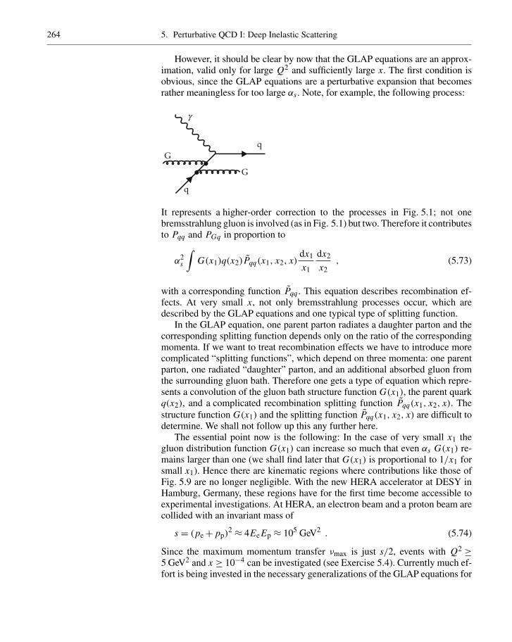
264 5. Perturbative QCD I: Deep Inelastic Scattering
However, it should be clear by now that the GLAP equations are an approx-imation, valid only for large Q2 and sufficiently large x. The first condition isobvious, since the GLAP equations are a perturbative expansion that becomesrather meaningless for too large αs. Note, for example, the following process:
It represents a higher-order correction to the processes in Fig. 5.1; not onebremsstrahlung gluon is involved (as in Fig. 5.1) but two. Therefore it contributesto Pqq and PGq in proportion to
α2s
∫G(x1)q(x2)Pqq(x1, x2, x)
dx1
x1
dx2
x2, (5.73)
with a corresponding function Pqq . This equation describes recombination ef-fects. At very small x, not only bremsstrahlung processes occur, which aredescribed by the GLAP equations and one typical type of splitting function.
In the GLAP equation, one parent parton radiates a daughter parton and thecorresponding splitting function depends only on the ratio of the correspondingmomenta. If we want to treat recombination effects we have to introduce morecomplicated “splitting functions”, which depend on three momenta: one parentparton, one radiated “daughter” parton, and an additional absorbed gluon fromthe surrounding gluon bath. Therefore one gets a type of equation which repre-sents a convolution of the gluon bath structure function G(x1), the parent quarkq(x2), and a complicated recombination splitting function Pqq(x1, x2, x). Thestructure function G(x1) and the splitting function Pqq(x1, x2, x) are difficult todetermine. We shall not follow up this any further here.
The essential point now is the following: In the case of very small x1 thegluon distribution function G(x1) can increase so much that even αs G(x1) re-mains larger than one (we shall find later that G(x1) is proportional to 1/x1 forsmall x1). Hence there are kinematic regions where contributions like those ofFig. 5.9 are no longer negligible. With the new HERA accelerator at DESY inHamburg, Germany, these regions have for the first time become accessible toexperimental investigations. At HERA, an electron beam and a proton beam arecollided with an invariant mass of
s = (pe+ pp)2 ≈ 4Ee Ep ≈ 105 GeV2 . (5.74)
Since the maximum momentum transfer νmax is just s/2, events with Q2 ≥5 GeV2 and x ≥ 10−4 can be investigated (see Exercise 5.4). Currently much ef-fort is being invested in the necessary generalizations of the GLAP equations for

5.2 An Alternative Approach to the GLAP Equations 265
small values of x. To this end their structure must be modified, as can alreadybe seen from (5.73). Terms have to be introduced, for example, that depend onproducts of two or more distribution functions. Up to now there has been no gen-erally accepted solution to this problem (Sect. 6.2). Presumably such a solutionwill only be found in connection with experimental investigations. The HERAexperiments have been producing data since 1992.
In this section we have learned how QCD corrections can be evaluated fromthe corresponding Feynman graphs. This procedure is of great clarity, but it re-quires extensive calculations. Therefore one frequently chooses another way toderive the GLAP equations that is much more elegant but unfortunately less ob-vious. The latter disadvantage occurs because a part of the result, namely thegeneral structure of the GLAP equations, has to be more or less assumed. Weshall discuss this alternative derivation in the following section, because it willshed additional light on the meaning of the GLAP equations.
5.2 An Alternative Approach to the GLAP Equations
In this section we shall be concerned with the derivation of the GLAP equationsusing only our knowledge about the properties of QCD.6 We know already thatscattering experiments using leptons as projectiles and hadrons as targets revealinformation about the hadronic structure. The structure functions or momentumdistributions of the partons inside the hadron depend on the four-momentum qµcarried by the exchanged photon (in general the vector meson). If the momentumtransfer Q2 is increased, more and more details of the hadronic structure becomevisible (see Fig. 5.10).
boost
Q2 small
Q2 large
_q
Fig. 5.10. The role of Q2 astransverse resolving power
Q2 is related to the maximum transverse momentum of a parton in the finalstate. This fact is easily understood by looking at Fig. 5.10. In the Breit frame,where the distribution functions are defined, the nucleon is strongly contracted inthe direction of movement. Therefore the resolution with which quarks are seendepends only on the transverse momentum. We denote by 1/
√Q2 the resolving
power, since hadronic structures down to 1/√
Q2 can be resolved owing to theHeisenberg inequality ∆x∆Q ∼ 1. Let us assume that we have chosen Q2 highenough to enter the perturbative regime. We can resolve partons of size 1/
√Q2
inside the hadron. If the momentum transfer is increased to Q′2 > Q2, one can
6 O. Nachtmann: Elementary Particle Physics (Springer, Berlin, Heidelberg 1990).

266 5. Perturbative QCD I: Deep Inelastic Scattering
resolve smaller constituents of size 1/√
Q′2 inside the hadron. For a given re-solving power 1/
√Q2 the momentum distribution of the partons of kind a is
denoted by Na(xa, Q2). The smaller constituents b at 1/√
Q′2 carry some of theparton momenta xa:
xb
xa< 1 . (5.75)
This results in a decrease in the momentum distribution for large x and an in-crease for small momentum fractions. In other words Na(xa, Q2) < Nb(xb, Q2).
The variation of the distribution functions ∆N(x, Q2) when Q2 is increasedby ∆Q2 can now be treated by using perturbation theory. To lowest order,∆N(x, Q2) is proportional to the coupling parameter
αs(Q2)= g2(Q2)
4π. (5.76)
If the quark masses are neglected, QCD lacks any energy scale. Therefore onlymomentum ratios can appear that govern the development of Na(xa, Q2) tohigher Q2. This distribution function for partons of kind a, i.e. Na(xa, Q2), de-pends for Q′2 > Q2 on the distribution of partons of all kinds b. We assume thisdependence to be linear. The probability of finding a parton a with momentumfraction xa inside a parton b of momentum fraction xb is therefore given by
∆Nb(xb, Q2)= αs(Q2)
2Pba
(xb
xa
)Na(xa, Q2)
∆Q2
Q2 . (5.77)
The quotient ∆Q2/Q2 =∆ ln Q2 is introduced to keep the change in momen-tum transfer dimensionless. In the same way it follows that Pba can only dependon the ratio of the momentum fractions. The factor 1
2 is convient.To obtain the total change of Nb we have to sum over all partons of kind a that
may “contain” the parton b, and we have to integrate over all parton momentaxa > xb. This leads us, finally, to the GLAP equations:
∆Nb(xb, Q2)= αs(Q2)
2π
∑b
1∫xb
Pba
(xb
xa
)Na(xa, Q2)
dxa
xa∆ ln Q2 . (5.78)
Here we have introduced the ratio dxa/xa instead of dxa alone; otherwise a scalewould enter the GLAP equations. One might wonder why a dimensionless inte-gration measure dxa/xb does not appear in (5.75). However, remember, the alsodimensionless integration measure dxa/dxb would lead to a splitting functionwith explicit dependence on single momenta and not only ratios. Equation (5.75)describes a set of equations for all types of partons, which in differential formbecomes
∂Nb(xb, Q2)
∂ ln Q2 = αs(Q2)
2π
∑b
1∫xb
Pba
(xb
xa
)Na(xa, Q2)
dxa
xa. (5.79)

5.2 An Alternative Approach to the GLAP Equations 267
The functions Pba are called splitting functions since they describe the breakingup of a parton of type a into partons of type b, when the momentum transfer Q2
is increased.In the following we will derive the splitting functions Pba for several cases.
Life is made easy by assuming that there are only two types of partons: quarksand gluons. Since we assume that all antiquarks are due to gluon splitting,G → qq, the increase in the number of quarks always equals the increase in thenumber of antiquarks. PqG = PuG = PuG = PdG = . . . . This is justified becauseof charge-conjugation symmetry (change in quark distribution equals change inantiquark distribution) and because of our treating quarks as massless objects(changes in u, d, s quarks proceeds in the same way). This reduces the numberof splitting functions to four:
Pqq =− 4
3(1+ x)+2δ(1− x)+ 8
3
⎛⎝ 1
1− x− δ(1− x)
1∫0
dx′ 1
1− x′
⎞⎠ ,
(5.80)
PqG =1
2
[(1− x)2+ x2
], (5.81)
PGq =4
3
1+ (1− x)2
x, (5.82)
PGG =6
[1
x−2+ x(1− x)
]+(
11
2− Nf
3
)δ(1− x)
+6
⎛⎝ 1
1− x− δ(1− x)
1∫0
dx′ 1
1− x′
⎞⎠ . (5.83)
We shall evaluate the functions PGq , Pqq , and PqG in Examples 5.5–5.7. Theeffect of these functions is depicted graphically in Fig. 5.11. The evaluation ofPGG can be found in other papers.7
EXERCISE
5.4 The Maximum Transverse Momentum
Problem. (a) Determine the maximum transverse momentum of a parton occur-ring in the final state if the photon momentum before the collision is given in theBreit system (see Exercise 3.6) by
qµ = (0; 0, 0,−Q) (1)
and the initial parton momentum in the Breit system is
pµ = (p; 0, 0, p) . (2)
7 See also, G. Altarelli: Partons in Quantum Chromodynamics, Phys. Rep. C 81, 1.
(a)
(b)
(c)
(d)
G,y
G,y
G,x-y
G,x-y
q,y
q,x-y
q,y
_x-yq,
q,x
q,x
G,x
G,x
Fig. 5.11a–d. The processesdescribed by the splittingfunctions (a) PGq , (b) Pqq ,(c) PqG , and (d) PGG

268 5. Perturbative QCD I: Deep Inelastic Scattering
Exercise 5.4 (b) Verify the relation νmax = s/2 and investigate the kinematical regionaccessible at the HERA collider.
Solution. (a) We first assume that two partons escape after the collision. Thesepartons carry momenta
p′1 =(
p
2; p⊥,
p−Q
2
),
p′2 =(
p
2;−p⊥,
p−Q
2
). (3)
Obviously the four-momentum is conserved:
q+ p = p′1+ p′2 . (4)
Furthermore squaring the parton momentum p′1 yields
(p′1)2 = 0 =( p
2
)2− (p⊥)2−(
p−Q
2
)2
=( p
2
)2− (p⊥)2−( p
2
)2+ 2p ·Q
4−(
Q
2
)2
=− (p⊥)2+ p ·Q
2−(
Q
2
)2
, (5)
because it is assumed to be of rest mass zero, i.e. p′12 = 0. Introducing the
momentum fraction x = Q2/(2p ·Q), one gets
− (p⊥)2−(
Q
2
)2
+ Q2
4x= 0 (6)
or
|p⊥| = Q
2
√1− x
x. (7)
For more than two partons in the final state this is the maximum transversemomentum that can be achieved.
(b) According to the definition (5.11), ν = q · pp, we have in the rest systemof the nucleon
νR.S.= (Ee− E′
e)Mp ,
νmax =Ee Mp . (8)
For the center-of-mass energy
s =(pp+ pe)2 = M2
p+2pp · pe+m2e ∼ 2pp · pe
R.S.= 2Ee Mp = 2νmax . (9)

5.2 An Alternative Approach to the GLAP Equations 269
From this we get for xmin
xmin = Q2
2νmax Q2
s. (10)
For HERA kinematics Ee = 30 GeV, E p = 820 GeV, so that
s eEe E p 105 GeV2 . (11)
Then we get for Q2 ∼ 5 GeV a minimal value xmin ∼ 10−4.
EXAMPLE
5.5 Derivation of the Splitting Function PGq
For given momentum transfer Q2 – in the perturbative region – we define theHamiltonian
HQ2 = HkinQ2 + V . (1)
The potential V describes the binding of the partons. It is the nonperturbativepart, including interactions with small Q2. The kinetic part Hkin
Q2 yields – whenapplied to the parton wave functions – the kinetic parton energies
HkinQ2 |qQ2(p) 〉 = E|qQ2(p) 〉 = |p||qQ2(p) 〉 ,
HkinQ2 |G Q2(k) 〉 = ω|G Q2(k) 〉 = |k||G Q2(k) 〉 . (2)
Here |qQ2(p) 〉 and |G Q2(k) 〉 denote the quark and gluon wave functions, respec-tively, at momentum transfer Q2. Again Q is related to the maximum transversemomentum by |k⊥|max ≡ |p⊥| of Exercise 5.4, (7), i.e.
|k⊥|max = Q
2
√1− x
x≡ εQ , ε= 1
2
√1− x
x. (3)
At Q′2 > Q2 the kinetic part of the Hamiltonian can be written as
HkinQ′2 = Hkin
Q2 + H∆Q2 . (4)
Application of HkinQ′2 to the quark and gluon wave functions at Q′2 again yields
HkinQ′2 |qQ′2(p) 〉 = |p||qQ′2(p) 〉 ,
HkinQ′2 |G Q′2(k) 〉 = |k||G Q′2(k) 〉 . (5)
The additional operator H∆Q2 just describes the interactions leading to trans-verse momenta |k⊥| between εQ and εQ′ (see Exercise 5.4).
Exercise 5.4

270 5. Perturbative QCD I: Deep Inelastic Scattering
Example 5.5 The interaction part of the QCD Hamiltonian can be derived in the temporalWeyl gauge, Aα0 = 0 for all gluons. The Hamiltonian H∆Q2 up to first order inthe coupling parameter g is
H∆Q2 =−g(Q2)
∫d3r
∑f,a
q f (r)[γ · Aa(r)
λa
2
]q f (r)
+ g(Q2)
∫d3r fabc Aa
j(r) Abk(r)
∂
∂r jAc
k(r) . (6)
This interaction Hamiltonian may be directly read off from Example 4.2, wherewe derived the Feynman rules (see (1) and (6) of Example 4.2). The additionalminus sign stems from the Legendre transformation that relates Lagrange andHamilton density. The first part describes the interaction between quarks and glu-ons, the second part handles the 3-gluon interaction. In the first part the sum isover all quark flavors u, d, s, . . . .
We turn now to the quark and gluon wave functions. Since for higher reso-lution (“virtuality”) Q′2 smaller constituents of the hadron can be seen, the wavefunction describing big partons at Q2 can be written as a superposition of wavefunctions for the constituents at Q′2. For the quark and gluon wave functionsat Q2 we get the expansion
|qQ2(p) 〉 =Cq(p)|qQ′2(p) 〉+∑k′,p′
CGq(k′, p′)|GQ′2(k′)qQ′2(p′) 〉 ,
|GQ2(k) 〉 =CG(k)|GQ′2(k) 〉+∑k′,p′
CqG(k′, p′)|GQ′2(k′)qQ′2(p′) 〉
+∑k′,k′′
CGG(k′, k′′)|GQ′2(k′)GQ′2(k′′) 〉 . (7)
The coefficients are given by
Cq(p)= 〈qQ′2(p)|qQ2(p) 〉 ,CG(k)= 〈GQ′2(k)|GQ2(k) 〉 ,
CGq(k′, p′)= 〈GQ′2(k′)qQ′2(p′)|qQ2(p) 〉 ,
CqG(k′, p′)= 〈GQ′2(k′)qQ′2(p′)|GQ2(p) 〉 ,
CGG(k′, k′′)= 〈GQ′2(k′)GQ′2(k′′)|GQ2(k) 〉 . (8)
The squared coefficients can be related to the momentum distribution functions.Note again that (7) describe the evolution of the various distribution functionfrom virtuality Q2 to virtuality Q′2. The whole evolution is calculated in first-order perturbation theory. Now we have all the ingredients to determine thesplitting functions. We start with the calculation of the probability of resolvinga gluon inside a quark (Fig. 5.11a). This will lead us to an expression for thesplitting function PGq .

5.2 An Alternative Approach to the GLAP Equations 271
We apply the kinetic part HkinQ′2 of the Hamiltonian to the quark wave function
at resolution Q2. This gives on the one hand
HkinQ′2 |qQ2(p) 〉 = Hkin
Q2 |qQ2(p) 〉+ H∆Q2 |qQ2(p) 〉= |p| |qQ2(p) 〉+ H∆Q2 |qQ2(p) 〉 . (9)
The expansion (7) of the quark wave function yields on the other hand
HkinQ′2 |qQ2(p) 〉= Cq(p)Hkin
Q′2 |qQ′2(p) 〉+∑k′,p′
CGq(k′, p′)Hkin
Q′2 |GQ′2(k′)qQ′2(p′) 〉
= Cq(p)|p| |qQ′2(p) 〉+∑k′,p′
(|k′|+ |p′|)CGq(k′, p′)|GQ′2(k′)qQ′2(p′) 〉 .
(10)
We project (9) onto the final-state wave function |GQ′2(k′)qQ′2(p′) 〉:|p|〈GQ′2(k′)qQ′2(p′)|qQ2(p) 〉+〈GQ′2(k′)qQ′2(p′)|H∆Q2 |qQ2(p) 〉= 〈GQ′2(k′)qQ′2(p′)|Hkin
Q′2 |qQ2(p) 〉= (|k′|+ |p′|)〈GQ′2(k′)qQ′2(p′)|qQ2(p) 〉= (|k′|+ |p′|)CGq(k
′, p′) , (11)
employing (5) and (8) as well as the orthogonality between the wave functions.Thus we obtain an expression for CGq:
CGq(k′, p′)= 〈GQ′2(k′)qQ′2(p′)|H∆Q2 |qQ2(p) 〉
|k′|+ |p′|− |p| . (12)
This is just first-order perturbation theory. The absolute square of this coefficientis proportional to the probability of finding a gluon of longitudinal momen-tum k′ inside a quark of momentum p when the resolution Q2 is increased. Themomentum fraction of the gluon relative to the quark is therefore
x = k′‖|p| =
k′ · p|p|2 . (13)
Starting with a single quark |qQ(p) 〉 and no gluons at the resolution Q2 we willhave initially a gluon distribution NG(Q2)= 0. Increasing the resolution fromQ2 to Q′2 we get due to Bremsstrahlung q → qG, at Q′2 the following distri-bution function (see Fig. 5.12). Averaging over the incoming quark spin s yields12
∑s, and therefore
NG(x, Q′2)=∑
a
1
2
∑ss′εa
∫d3 p′
(2π)32E′
∫d3k′
(2π)32ω′
× δ(
x− k′ · p|p|2
)|CGq(k
′, p′)|2 1
2E, (14)
Example 5.5
p ,s p ' ,s'
k ' ,εa
Fig. 5.12. Bremsstrahlungof a gluon by a quark. Thequark wave function is nor-malized within the volumeV according to 1/
√2EV
×u(p, s)eipx . s, s′ denotethe spin of the quark be-fore and after the scattering,respectively. εa is the polar-ization vector of the gluon

272 5. Perturbative QCD I: Deep Inelastic Scattering
Example 5.5 where the k integration is performed for |k⊥| in the range from εQ2 to εQ′2. Here∫d3 p′/(2π)32E′ and
∫d3k′/(2π)32ω′ are the invariant phase-space factors (see
(2.115)). The factor 1/2E stems from the normalisation of the incoming quarkwave function. The eight color degrees of freedom of the gluons are enumeratedby a. We now evaluate the squared coefficient |CGq(k′, p′)|2. To do this, only thefirst part of Hamiltonian (6) is required. Inserting (6) into (12) yields
CGq(k′, p′)=− g(Q2)
∫d3r
∑f
〈G Q′2(k′)qQ′2(p′)|q f (r)
×(
γ · Aa(r)λa
2
)q f (r)|qQ2(p) 〉 1
|k′|+ |p′|− |p|=− g(Q2)δ3(k′ + p′ − p)(2π)3u(p′, s′)ε a∗ ·γ λ
a
2u(p, s)
× 1
|k′|+ |p′|− |p| . (15)
Note that the quark spinors u(p, s) are here defined without the normalizationfactor 1/
√2EV . The latter is explicitely denoted in (14) within the invari-
ant phase space factors. Again it is obvious that CGq(k′, p′) is calculated infirst-order perturbation theory (see also Fig. 5.12). From this it follows that
NG(x, Q′2)=∫
d3 p′
(2π)3
∫d3k′
(2π)31
8EE′ω′δ
(x− k′ · p
|p|2)
× δ3(k′ + p′ − p)(2π)3g(Q2)2 1
(|k′|+ |p′|− |p|)2
× 1
2
∑a
∑s,s′,εa
∣∣∣∣u(p′, s′)(ε a∗ ·γ )λa
2u(p, s)
∣∣∣∣ 2
. (16)
Here [δ3(k′ + p′ − p)]2 = (2π)3Vδ3(k′ + p′ − p) has been used and the normal-ization volume V is set to V = 1. We consider the expression for the squaredmatrix element. Performing the summation over color and spin, where we haveused the relation ε/a =−ε a ·γ for εa = (0, ε a), we get
1
2
∑s
1
3
∑c
∑a
∑εa
∑s′,c′
∣∣∣∣uc′(p′, s′)ε/a λacc′2
uc(p, s)
∣∣∣∣2
= 1
6
∑s,s′
∑c,c′
∑εa
∑a,a′
tr
[ε/a λ
acc′2
uc′(p, s)uc′(p, s)λa′
c′c2ε/a′uc(p, s)uc(p, s)
],
where c, c′ denote the colors of the quarks. Performing the sums over spins andover colors∑
s
uc′(p, s)uc′(p, s)= p/+m ≈ p/ ,
∑c,c′
λacc′2
λa′c′c2
= trλa
2
λa′
2= 1
2δaa′ ,

5.2 An Alternative Approach to the GLAP Equations 273
we obtain
2 · 1
6
∑εa
∑a
tr
p/′ε/a∗ p/ε/a= 1
6
∑a
∑εa
1
2·4 [(p′ · εa∗)(p · εa)+ (p′ · εa)(p · εa∗)− (p · p′)(εa · εa∗)
]= 1
3
∑a
∑εa
[(p′ ·ε a∗)(p ·ε a)
+ (p′ ·ε a)(p ·ε a∗)− (p′0 p0− (p′ · p))(ε a ·ε a∗)]
= 1
3
∑a
∑εa
(εa)i(εa∗) j
pi p′j + p′i p j −
[(p′ · p)−|p||p′|] δij
= 1
38 ·(δij −
k′ik′j|k′|2
)pi p′j + p′i p j −
[(p′ · p)−|p||p′|] δij
= 16
3
1
|k′|2 [|p||p′||k′|2− (k′ · p)(k′ · p′)] , (17)
where we summed over transversal polarisations of the gluon with momentum k′
∑a
∑εa
(εa)i(εa∗) j = 8
∑ε
εiε∗j = 8
(δij −
k′ik′j|k′|2
).
Inserting this into (16) yields
NG
(x, Q′2)=2
3
1
(2π)3g2(Q2)
∫d3 p′
∫d3k′ 1
EE′ω′δ
(x− k′ · p
|p|2)
× δ3(k′ + p′ − p) · 1
(|k′|+ |p′|− |p|)2× 1
|k′|2 [|p||p′||k′|2− (k′ · p)(k′ · p′)] . (18)
The momenta can be written as (see Fig. 5.11)
p =(0, 0, p) ,
k′ =(k′⊥, x p) ,
p′ =(−k′⊥, (1− x)p) . (19)
Obviously the three-momentum is conserved: p = k′ + p′. The transverse mo-mentum is expected to be small compared to the longitudinal momenta:
|k′⊥| p , |k′⊥| x p , |k′⊥| (1− x)p . (20)
Example 5.5

274 5. Perturbative QCD I: Deep Inelastic Scattering
Example 5.5 The term 1|k′|+|p′|−|p| in the expression NG(x, Q2) of (18) can be approximated
by
|k′|+ |p′|− |p| ≈ x p+ |k′⊥|22x|p| + (1− x)p+ |k′⊥|2
2(1− x)|p| − |p|
= |k′⊥|22p
1
x(1− x), (21)
and therefore
1
|k′|+ |p′|− |p| ≈2p
|k′⊥|2x(1− x) .
Furthermore
1
|k′|2[|p||p′||k′|2− (k′ · p)(k′ · p′)
]≈ 1
x2 p2
[p(1− x)p(|k′⊥|2+ x2 p2)
+ 1
2(1− x)p2 |k′⊥|p(|k′⊥|2+ x2 p2)+ x p2|k′⊥|2− x2 p2(1− x)p2]
=|k′⊥|2x2
[1+ x2
2(1− x)
](22)
and
1
EE′ω′= 1
|p||p′||k ′| ≈1
p3x(1− x). (23)
Inserting (21)–(23) into the gluon distribution (18) results in
NG(x, Q′2)=2
3
1
(2π)3g2(Q2)
∫d3k′
∫d3 p′
× δ(
x− k′ · p|p|2
)δ3(k′ + p′ − p)
1
p3x(1− x)
× 4p2
|k′⊥|4x2(1− x)2 · |k
′⊥|2x2
(1+ x2
2(1− x)
)
=4
3
1
(2π)3g2(Q2)
1+ (1− x)2
x
∫d2k′⊥|k′⊥|2
. (24)
In the last step we wrote d3k′ = d2k′⊥ dk‖ and performed the integration over p′and k‖, thus cancelling the δ functions.

5.2 An Alternative Approach to the GLAP Equations 275
The last integration has to be performed for transverse momenta |k′⊥| betweenεQ and εQ′ (see (3)–(5) and Exercise 5.4):
εQ′∫εQ
d2k′⊥|k′⊥|2
= 2π
εQ′∫εQ
dk′⊥|k′⊥|
= 2π ln |k′⊥|
∣∣∣∣∣∣∣εQ′
εQ
= 2π(ln εQ′ − ln εQ)
= π(ln ε2 Q′2− ln ε2 Q2)
= π∆ ln ε2 Q2 = π∆ ln Q2 . (25)
Q2 is preferred in the argument of the logarithm, because it is this quantitywhich enters the GLAP equations (5.75) and (5.76). Since ε was introduced asan arbitrary constant ∆ ln ε= 0. We are left with
NG(x, Q2)= g2(Q2)
8π2
4
3
1+ (1− x)2
x∆ ln Q2 . (26)
Here we introduced again Q2 instead of Q′2 in the argument of NG(x, Q2), be-cause Q′2 is hidden in ∆ ln Q2 – see (25). Both notations will be used in thefollowing. This result now has to be compared to the GLAP equation (5.76),where we have to impose the initial condition
Nq(x, Q2)= δ(1− x) ,
NG(x, Q2)= 0 , (27)
which is in accordance with the initial quark state |qQ2(p) 〉 in (12) where glu-ons are absent. From this condition we evolve the parton distribution function toNG(x, Q2). The term “initial condition” has to be understood in that way thatone has distribution functions at a virtuality Q2, from which one determines thedistribution functions at the higher virtuality Q′2 > Q2.
From the GLAP equations (5.76) it follows that
NG(x, Q′2)= NG(x, Q2)+∆NG(x, Q2)
=∆NG(x, Q2)
= g2
8π2 PGq(x)∆ ln Q2 . (28)
Therefore we can conclude that
∆NG(x, Q2)= g2
8π2 PGq(x)∆ ln Q2 (29)
with the PGq splitting function given by
PGq(x)= 4
3
1+ (1− x)2
x. (30)
Example 5.5

276 5. Perturbative QCD I: Deep Inelastic Scattering
G,(1- )x
q,x
Fig. 5.13.
EXAMPLE
5.6 Derivation of the Splitting Function Pqq
Up to now we have determined only the gluon distribution function NG(x, Q′2)(see (28) of Example 5.5). To determine the quark momentum distributionNq(x, Q′2) we have to keep in mind that the production of a quark of momen-tum fraction x corresponds to the production of a gluon of momentum fraction1− x (see Fig. 5.13). For x = 1 the original quark is obtained with a probability|Cq(p)|2. We can therefore write
Nq(x, Q′2)= Nq(x, Q2)+∆Nq(x, Q2)
=∆NG(1− x, Q2)+ δ(1− x)|Cq(p)|2 . (1)
The first term on the right-hand side denotes the probability for having a gluonwith virtuality Q2 and momentum fraction 1− x; the second term describesthe probability for having no gluon at all. The change in the quark distributionfunction is then given by (see (27) of Example 5.5)
∆Nq(x, Q2)= Nq(x, Q′2)− Nq(x, Q2)= Nq(x, Q′2)− δ(1− x)
=∆NG(1− x, Q2)− δ(1− x)[1−|Cq(p)|2
]. (2)
∆NG(1− x, Q2) is already known from Example 5.5. Furthermore the longitu-dinal momentum is conserved. In other words, the longitudinal momentum ofthe newly created quarks, x∆Nq(x, Q2), together with the total longitudinal mo-mentum of the created gluons, x∆NG(x, Q2), should vanish, i.e. the expectationvalue of the longitudinal momentum should equal zero:
1∫0
dx x(∆Nq(x, Q2)+∆NG(x, Q2))= 0 . (3)
If we use the result of the last section, that the change in the gluon distributionis given by the splitting function PGq ,
∆NG(1− x, Q2)= g2(Q2)
8π2
4
3
1+ x2
1− x∆ ln Q2 ,
∆NG(x, Q2)= g2(Q2)
8π2
4
3
1+ (1− x)2
x∆ ln Q2 , (4)
momentum conservation allows us to determine the coefficient |Cq(p)|2:
0 =1∫
0
dx x[∆NG(1− x, Q2)− δ(1− x)(1−|Cq(p)|2)+∆NG(x, Q2)
](5)

5.2 An Alternative Approach to the GLAP Equations 277
or
|Cq(p)|2 = 1−1∫
0
dx x[∆NG(1− x, Q2)+∆NG(x, Q2)
]
= 1− g2(Q2)
8π2 ∆ ln Q2 4
3
1∫0
dx x
(1+ (1− x)2
x+ 1+ x2
1− x
)
= 1− g2(Q2)
8π2 ∆ ln Q2
⎛⎝8
3
1∫0
dx1
1− x−2
⎞⎠ . (6)
Finally we get for the change in the quark distribution (2)
∆Nq(x, Q2)= g2(Q2)
8π2 ∆ ln Q2
⎡⎣4
3
1+ x2
1− x+2δ(1− x)
− 8
3δ(1− x)
1∫0
dx′ 1
1− x′
⎤⎦ . (7)
Comparing this to the GLAP equation (see (28) in the previous example, whichcan be directly translated into a similar equation for ∆Nq; see also (5.74)),
∆Nq(x, Q2)= g2(Q2)
8π2 Pqq(x)∆ ln Q2 , (8)
allows us to extract the splitting function
Pqq = 4
3
1+ x2
1− x+2δ(1− x)− 8
3δ(1− x)
1∫0
dx′ 1
1− x′
= −4
3(x+1)+2δ(1− x)+ 8
3
⎛⎝ 1
1− x− δ(1− x)
1∫0
dx′ 1
1− x′
⎞⎠ . (9)
EXAMPLE
5.7 Derivation of the Splitting Function PqG
Next we calculate the splitting function that describes the quark fraction insidea gluon when the resolving power is increased from Q2 to Q′2 (Fig. 5.11c). Thefinal-state wave function is given by
|q′Q′2(p)qQ′2(p′) 〉 . (1)
Example 5.6

278 5. Perturbative QCD I: Deep Inelastic Scattering
Example 5.7 The initial gluon wave function at Q2 can be expanded into these quarks states:
|G Q2(k) 〉 =∑p,p′
Cqq(p, p′)|qQ′2(p)qQ′2(p′) 〉 , (2)
where the coefficients are given by
Cqq(p, p′)= 〈qQ′2(p)qQ′2(p′)|G Q2(k) 〉 . (3)
Applying the kinetic part of the Hamiltonian (see (4) of Example 5.5) yields
HQ2 |G Q2(k) 〉+∆HQ2 |G Q2(k) 〉 =∑p,p′
Cqq(p, p′)HQ′2 |qQ′2(p)qQ′2(p′) 〉
(4)
or
k|G Q2(k) 〉+∆HQ2 |G Q2(k) 〉=∑p,p′
(|p|+ |p′|)×Cqq(p, p′)|qQ′2(p)qQ′2(p′) 〉 . (5)
The coefficients can be obtained by projecting with 〈qQ′2(p)qQ′2(p′)|:
Cqq(p, p′)= 〈qQ′2(p)qQ′2(p′)|∆HQ2 |G Q2(k) 〉|p|+ |p′|− |k| . (6)
To determine Cqq(pp′) we need from the Hamiltonian ∆HQ2 (see (6) ofExample 5.5) the part that describes the quark–gluon interaction:
∆HQ2 =−g2(Q2)∑
a
∫d3x
∑f
q f (r)Aa(r)γ
λa
2q f (r) . (7)
As in (15) in Example 5.5 it follows for the matrix element that
〈qQ′2(p)qQ′2(p′)|∆HQ2 |G Q2(k) 〉= −
∑a
g(Q2)(2π)3δ3(p+ p′ −k)u(p, s)ε a ·γ λa
2v(p′, s′) . (8)
Again we can relate the squared coefficient Cqq(p, p′) to the quark distri-bution function by calculating the “decay probability” of a gluon if the re-solving power Q2 is increased. Following our previous calculation (see (14)of Example 5.5) we start with a single gluon |G Q2(k) 〉 and no quarks at theresolution Q2. Increasing the resolution to Q′2 will generate quarks throughthe process of pair production and we obtain the following quark distributionfunction:
∆Nq(c, Q′2)=1
8
∑a
1
2
∑εa
∑c s
∑c′s′
1
2ω
∫d3 p
(2π)32E
∫d3 p′
(2π)32E′
× δ(
x− p ·k|k|2
)|Cqq(p, p′)|2 . (9)

5.2 An Alternative Approach to the GLAP Equations 279
This is summed over spins (s, s′) and colors (c, c′) (factor 1/8) of the outgoingquarks and it is averaged over the spin εa (factor 1/2) and color of the initialgluon. Remenber that the gluon, being a vector particle, has spin 1. However,being massless, the gluon has only two (transverse) spin directions, as is the casefor the photon. The δ function guarantees that the quark longitudinal momentumis x times the gluon momentum:
x = p′′
|k| =p ·k|k|2 . (10)
Inserting Cqq(p, p′) from (6) into (9), we find that (9) becomes
∆Nq(c, Q2)= g(Q2)21
16(2π)3
∫d3 p
(2π)3
∫d3 p′
(2π)3
× δ(
x− p ·k|k|2
)δ3(p+ p′ −k)
1
8ωEE′
(1
|p|+ |p′|− |k|)2
×∑
a
∑εa
∑c s
∑c′s′
|uc(p, s)ε a ·γ λa
2vc′ A(p′, s′)|2 . (11)
We first perform the spin and color summations, again using ε/a =−γ ·ε for εa =(0, ε a):
∑a
∑εa
∑c s
∑c′s′
|uc(p, s)ε a ·γ λa
2vc′(p′, s′)|2
=∑a,b
tr
(λaλb
4
)∑εa
tr[p/(ε a ·γ )p/′(ε b∗ ·γ )]
=∑
a
1
2
∑εa
tr(
p/ε/a p/′ε/a∗)=∑
a
1
2
∑εa
4 · [(p · εa)(p′ · εa∗)+ (p′ · εa)(p · εa∗)− (p · p′)(εa · εa∗)]
= 2∑
a
∑εa
[(p ·ε a)(p′ ·ε a∗)
+ (p′ ·ε a)(p ·ε a∗)− (p0 p′0− p · p′)(ε a ·ε a∗)]
= 16
(δij − kik j
|k|2)(pi p′j + p′i p j + (|p||p′|− p · p′)δij)
= 32
|k|2[|k|2|p||p′|− (k · p)(k · p′)
]. (12)
Example 5.7

280 5. Perturbative QCD I: Deep Inelastic Scattering
Example 5.7 The summation over the colors a is performed exactly the same way as was donein Example 5.5, (17). The quark distribution function can now be written as
∆Nq(c, Q2)= g(Q2)21
4(2π)3
∫d3 pδ
(x− p ·k
|k|2)
1
8ωEE′ (13)
×(
1
|p|+ |p′|− |k|)2 1
|k|2 (|k|2|p||p′|− (k · p)(k · p′)) .
Here p′ = k− p is due to the δ3(p+ p′ −k) function. This conservation of thethree-momentum will now be handled explicitly. We introduce explicit forms forthe gluon and quark momenta,
k= (0, 0, k) ,
p = (k⊥, xk) ,
p′ = (−k⊥, (1− x)k) , (14)
so that the three-momentum is conserved: k= p+ p′. As in the last sections wetake |k⊥| to lie between εQ and εQ′ and assume that all momenta are muchgreater than |k⊥|2:
|k| |k⊥| , |p| |k⊥| , |p′| |k⊥| . (15)
The terms that enter (13) can now be approximated as in previous sections (see(25) in Example 5.5):
1
|p|+ |p′|− |k| =1√
k2⊥+ x2k2+√
k2⊥+ (1− x)2k2−|k|= 2k
|k⊥| x(1− x) , (16)
1
ωEE′ =1
x(1− x)k3 , ω= k , (17)
1
|k|2 (|k|2|p||p′|− (k · p)(k · p′))= 1
2|k⊥|2 (1− x)2+ x2
x(1− x). (18)
Inserting these expressions into (13) and rewriting
d3 p = d2k⊥ dp‖ (19)
we can perform the integration over the longitudinal momentum, obtaining
∆Nq(x, Q′2)= g(Q2)2
8π3
∫d2k⊥|k⊥|2
1
2
((1− x)2+ x2
)= g(Q2)2
4π2
∫dk⊥|k⊥|
1
2
((1− x)2+ x2
). (20)

5.3 Common Parametrizations of the Distribution Functions and Anomalous Dimensions 281
Keeping in mind that |k⊥| is in the range εQ to εQ′, we can perform the lastintegration. The result is
∆Nq(x, Q′2)= g(Q2)2
4π2
1
2
((1− x)2+ x2
)ln |k⊥|
∣∣∣∣εQ′
εQ
= g(Q2)2
8π2
1
2
((1− x)2+ x2
)∆ ln Q2 , (21)
since ε is an arbitrary constant∆ ln ε = 0. Comparing this result with the GLAPequation (see (5.74)) yields, with the initial condition
NG(x, Q2)= δ(1− x) , Nq(x, Q2)= 0 , (22)
the expression for the splitting function:
PqG(x)= 1
2
((1− x)2+ x2
). (23)
5.3 Common Parametrizations of the Distribution Functionsand Anomalous Dimensions
Instead of dealing with the GLAP equations (5.76) we can transform the set ofintegral equations into a set of linear equations by introducing the moments ofthe structure functions. The nth moment is defined as8
Ma(n, Q2)=1∫
0
dx xn−1 Na(x, Q2) , (5.84)
where Na is the structure function of the parton of kind a. Differentiating thiswith respect to ln(Q2) and inserting the GLAP equations (5.76) results in
dMa(n, Q2)
d ln Q2 =1∫
0
dx xn−1 dNa(x, Q2)
d ln Q2
=1∫
0
dx xn−1 g2(Q2)
8π2
∑b
1∫x
dx′
x′Pab
( x
x′)
Nb(x′, Q2)
= g2s (Q
2)
8π2
∑b
1∫0
dx xn−1
1∫x
dx′
x′Pab
( x
x′)
Nb(x′, Q2) .
(5.85)
8 Usually one defines the nth moment as the expectation value of xn rather than xn−1,which is commonly chosen in QCD.
Example 5.7

282 5. Perturbative QCD I: Deep Inelastic Scattering
The second integration over x′ between x and 1 can be performed from x′ = 0to x′ = 1 if one introduces the Heavyside function in the integrand. Thus theintegrand vanishes for x′ < x:
dMa(n, Q2)
d ln Q2 =g2(Q2)
8π2
∑b
⎛⎝ 1∫0
dx xn−1
×1∫
0
dx′
x′Pab
( x
x′)Θ(x′ − x)Nb(x
′, Q2)
⎞⎠ . (5.86)
Now the integrations can be exchanged. Substituting z = x/x′ we get
dMa(n, Q2)
d ln Q2 = g2(Q2)
8π2
∑b
⎛⎜⎝ 1∫0
dx′
x′Nb(x
′, Q2)
×1∫
0
dx xn−1 Pab
( x
x′)Θ(x′ − x)
⎞⎠= g2(Q2)
8π2
∑b
⎛⎜⎝ 1∫0
dx′
x′Nb(x
′, Q2)
×1/x′∫0
dz x′ (zx′)n−1 Pab(z)Θ(x′ − x′z)
⎞⎟⎠= g2(Q2)
8π2
∑b
⎛⎜⎝ 1∫0
dx′x′n−1 Nb(x′, Q2)
×1/x′∫0
dz zn−1 Pab(z)Θ(1− z)
⎞⎟⎠= g2(Q2)
8π2
∑b
1∫0
dx′x′n−1 Nb(x′, Q2)
1∫0
dz zn−1 Pab(z) .
(5.87)
The last step can be performed since 1/x′ ≥ 1 (because x′ ≤ 1 ) and theΘ function contributes only for z = 1/x′ ≤ 1 . Therefore the upper bound of theintegration can be taken as 1.

5.3 Common Parametrizations of the Distribution Functions and Anomalous Dimensions 283
In the high-Q2 regime αs(Q2)= gs(Q2)2/4π is given in leading-log order(see (4.147) which has to be taken at µ2 = Q2) by
αs(Q2)= 12
33−2Nf
π
ln(Q2/Λ2), (5.88)
where Nf denotes the number of quark flavors and Λ is the QCD cut-offparameter. We obtain (see Example 4.4)
dMa(n, Q2)
d ln Q2 = 6
33−2Nf
1
ln(Q2/Λ2)
∑b
Mb(n, Q2)
1∫0
dz zn−1 Pab(z)
=− 1
ln(Q2/Λ2)
∑b
Mb(n, Q2)dab(n) , (5.89)
where we have abbreviated the moment of the splitting function Pab(z) by
dab(n)=− 6
33−2Nf
1∫0
dz zn−1 Pab(z) . (5.90)
Thus we have derived a system of linear equations between the moments of thestructure functions and their derivatives. The moments dab(n) of the splittingfunctions are the anomalous dimensions. We shall come back to that in the dis-cussion of the renormalization group (Sect. 5.4). Once the splitting functions aregiven, the moments dab(n) can easily be obtained (see Exercise 5.8):
dGq(n)=− 8
33−2Nf
n2+n+2
n(n2−1),
dqq(n)= 4
33−2Nf
⎛⎝1− 2
n(n+1)+4
n∑j=2
1
j
⎞⎠ ,
dqG(n)=− 3
33−2Nf
n2+n+2
n(n+1)(n+2),
dGG(n)= 9
33−2Nf
⎛⎝1
3+ 2Nf
9− 4
n(n−1)− 4
(n+1)(n+2)+4
n∑j=2
1
j
⎞⎠ .
(5.91)
The moments M(n, Q2) of the parton distributions N(x, Q2) are given by experi-ment. However, it is more difficult to calculate the parton distributions N(x) forgiven moments M(n). Here we deleted the Q2 dependence in the argument, be-cause the relation between the distribution function N(x, Q2) and the momentaM(n, Q2) is shown at the renormalization point Q2 = µ2. At this special pointthe Q2 dependence drops out. After N(x, Q2 = µ2) is known one may obtainN(x, Q2) at any other Q2 by applying the GLAP evolution; see, e.g., (5.86).

284 5. Perturbative QCD I: Deep Inelastic Scattering
Since the polynomials xn do not form an orthonormal system of functions in therange 0 ≤ x ≤ 1, one has to transform the moments M(n) into coefficients
ci = f(M(n)
), (5.92)
so that
N(x)=∑
i
ci xi . (5.93)
The coefficients ci are functions of the moments N(n) and can be obtained fromthe relation
M(n)=∑
i
1
i+nci , (5.94)
which is proven as follows.Let f(x) be the function that is to be approximated by g(x)=∑
i ci xi . Againthe moments of f(x) are denoted by
fn =1∫
0
dx xn−1 f(x) . (5.95)
We require that
M =1∫
0
dx(
f(x)− g(x))2 (5.96)
becomes minimal, in which case the variation of M with respect to the coeffi-cients ck vanishes:
0 = δM = ∂M
∂ckδck , (5.97)
from which it follows that
∂M
∂ck= 0 for all k . (5.98)
Inserting the series expansion for g(x) into (5.93), we can express M by thecoefficients ci and the moments f :
M =1∫
0
dx
(f(x)2+ g(x)2−2 f(x)g(x)
)
=1∫
0
dx f(x)2+1∫
0
dx g(x)2−2
1∫0
dx f(x)g(x)

5.3 Common Parametrizations of the Distribution Functions and Anomalous Dimensions 285
= C+∑i, j
cic j
1∫0
dx xi+ j −2∑
i
ci
1∫0
dx xi f(x)
= C+∑i, j
cic j
i+ j+1−2
∑i
ci fi+1 . (5.99)
C = ∫ 10 dx f(x)2 is a constant.
Performing the derivation with respect to ck we get the desired relationbetween the coefficients ci and the moments fi of the function f :
0 = ∂M
∂ck
= ∂
∂ck
(C+
∑i, j
cic j
i+ j+1−2
∑i
ci fi+1
)=∑i, j
∂
∂ck
cic j
i+ j+1−2
∑i
∂ci
∂ckfi+1
=∑i, j
δikc j + ciδ jk
i+ j+1−2
∑i
δik fi+1
= 2∑
i
ci
i+ k+1−2 fk+1 , (5.100)
or
fk =∑
i
ci
i+ k≡∑
i
Akici . (5.101)
In order to compute the coefficients ci from the known moments fk, one has todetermine the inverse of the matrix Aki :
ci =(
A−1)
ikfk . (5.102)
Obviously the coefficients ci change their values if one more moment fk is addedin the calculation.
It is possible to give an upper and lower bound to f(x) by employing thePade approximation method for the moments fk.9 Recent parametrizations forthe parton distributions inside the nucleon are given by CTEQ. (The CTEQ groupprovides continuously updated sets of distribution functions, obtainable viaWWW from http://www.phys.psu.edu/˜cteq/, which is regularly updated.) Herewe give another parametrization.10 Writing for s in a leading-log approximation
s = lnln[Q2/(0.232 GeV)2
]ln[µ2/(0.232 GeV)2
] , (5.103)
9 W.W. Press, B.P. Flannery, S.A. Teukolsky, W.T. Vetterling: Numerical Recipes (Cam-bridge University Press 1992)
10 M. Glück, E. Reya, A. Vogt: Z. Physik C 53, 127 (1992)

286 5. Perturbative QCD I: Deep Inelastic Scattering
whereµ2 = 0.25 GeV2, the parton distributions are parametrized as follows. Thedistribution function for the u and d valence quarks in a proton are denoted byvp(x, Q2). We use the parametrization
xvp(x, Q2)= Nxa(1+ A√
x+ Bx)(1− x)D , (5.104)
with
N = 0.663+0.191s−0.041s2+0.031s3 ,
a = 0.326 ,
A =−1.97+6.74s−1.96s2 ,
B = 24.4−20.7s+4.08s2 ,
D = 2.86+0.70s−0.02s2 , (5.105)
for v= uv+dv and
N = 0.579+0.283s+0.047s2 ,
a = 0.523−0.015s ,
A = 2.22−0.59s−0.27s2 ,
B = 5.95−6.19s+1.55s2 ,
D = 3.57+0.94s−0.16s2 , (5.106)
for v= dv. The distributions for a neutron are obtained by interchanging u andd quarks.
The gluon and light-sea-quark distributions are given by
xwp(x, Q2)=[
xα(
A+ Bx+Cx2)
ln
(1
x
)b
+sα exp
(−E+
√E′sβ ln
(1
x
))](1− x)D , (5.107)
with
α= 0.558 ,
β = 1.218 ,
a = 1.00−0.17s ,
b = 0 ,
A = 4.879s−1.383s2 ,
B = 25.92−28.97s+5.596s2 ,
C =−25.69+23.68s−1.975s2 ,
D = 2.537+1.718s+0.353s2 ,
E = 0.595+2.138s ,
E′ = 4.066 (5.108)

5.3 Common Parametrizations of the Distribution Functions and Anomalous Dimensions 287
for w= G and
α= 1.396 ,
β = 1.331 ,
a = 0.412−0.171s ,
b = 0.566−0.496s ,
A = 0.363 ,
B =−1.196 ,
C = 1.029+1.785s−0.459s2 ,
D = 4.696+2.109s ,
E = 3.838+1.944s ,
E′ = 2.845 (5.109)
for w= u and w= d, characterizing the light sea quarks. Finally for the s, c, bquark distributions, we employ the relation
xw′p(x, Q2)= (s− sw′)α
[ln(1/x)]a(1+ A
√x+ Bx
)(1− x)D
×exp
(−E+
√E′sβ ln
(1
x
)), (5.110)
where the s-quark distribution is given by
α= 0.803 ,
β = 0.563 ,
a = 2.082−0.577s ,
A =−3.055+1.024s0.67 ,
B = 27.4−20.0s0.154 ,
D = 6.22 ,
E = 4.33+1.408s ,
E′ = 8.27−0.437s ,
sw′ = ss = 0 . (5.111)
The c, c distribution is parametrized by
α= 1.01 ,
β = 0.37 ,
a = 0 ,
A = 0 ,
B = 4.24−0.804s ,
D = 3.46+1.076s ,

288 5. Perturbative QCD I: Deep Inelastic Scattering
E = 4.61+1.49s ,
E′ = 2.555+1.961s ,
sw′ = sc = 0.888 , (5.112)
and the b,b distribution by
α= 1.00 ,
β = 0.51 ,
a = 0 ,
A = 0 ,
B = 1.848 ,
D = 2.929+1.396s ,
E = 4.71+1.514s ,
E′ = 4.02+1.239s ,
sw′ = sb = 1.351 . (5.113)
The parametrizations are valid in the x range
10−5 ≤ x < 1 (5.114)
and the scale
µ2 ≤ Q2 ≤ 108 GeV2 (5.115)
with an averaged inaccuracy of 2%−3%.
EXERCISE
5.8 Calculation of Moments of Splitting Functions(Anomalous Dimensions)
Problem. Calculate the moments of the splitting functions PGq , Pqq , PqG , andPGG . The splitting functions are explicitly (see (5.70)–(5.72))
(a) PGq = 4
3
1+ (1− x)2
x,
(b) Pqq =−4
3(1+ x)+2 δ(1− x)
+ limε→0
8
3
[1
1− x+ε − δ(1− x)
1∫0
dy1
1− y+ε],

5.3 Common Parametrizations of the Distribution Functions and Anomalous Dimensions 289
(c) PqG = 1
2
[x2+ (1− x)2
],
(d) PGG = 6
[1
x−2+ x(1− x)
]+(
11
2− Nf
3
)δ(1− x)
+ limε→0
6
[1
1− x+ε − δ(1− x)
1∫0
dy1
1− y+ε].
Solution. (a) Inserting the explicit expression for the splitting function PGq weget for the nth moment
dGq(n)=− 6
33−2Nf
1∫0
dx xn−1 PGq(x)
=− 6
33−2Nf
1∫0
dx xn−1 4
3
1+ (1− x)2
x
=− 8
33−2Nf
1∫0
dx(
2xn−2−2xn−1+ xn)
=− 8
33−2Nf
(2
n−1x n−1− 2
nxn + 1
n+1xn+1
)∣∣∣∣10. (1)
Since n ≥ 1 we get
dGq(n)=− 8
33−2Nf
(2
n−1− 2
n+ 1
n+1
)=− 8
33−2Nf
n2+n+2
n(n2−1). (2)
(b) The nth moment of the splitting function Pqq is given by
dqq(n)=− 6
33−2Nf
1∫0
dx xn−1 Pqq(x)
=− 6
33−2Nf
1∫0
dx xn−1[− 4
3(1+ x)+2δ(1− x)
+ limε→0
8
3
(1
1− x+ε − δ(1− x)
1∫0
dy1
1− y+ε)]
Exercise 5.8

290 5. Perturbative QCD I: Deep Inelastic Scattering
Exercise 5.8
=− 6
33−2Nf
[− 4
3
1∫0
dx(xn−1+ xn)+2
+ limε→0
8
3
( 1∫0
dxxn−1
1− x+ε −1∫
0
dy1
1− y+ε)]
. (3)
With the expansion
xn−1
1− x+ε =−n−2∑i=0
xi + 1
1− x+ε (4)
this equation can be put into a simple form:
dqq(n)=− 6
33−2Nf
[− 8
3
n∑i=0
1∫0
dx xi + 4
3
1∫0
dx(xn−1+ xn)+2
]
=− 6
33−2Nf
[− 8
3
n∑i=0
1
i+1+ 4
3
(1
n+ 1
n+1
)+2
]
=− 6
33−2Nf
[− 8
3
n∑i=2
1
i− 8
3
1
n+1− 8
3+ 4
3
1
n+ 4
3
1
n+1+2
]
= 4
33−2Nf
[4
n∑i=2
1
i+1− 2
(n+1)n
]. (5)
(c) For the moment dqG(n) we get
dqG(n)=− 6
33−2Nf
1∫0
dx xn−1 PqG(x)
=− 6
33−2Nf
1∫0
dx xn−1 1
2
[x2+ (1− x)2
]
=− 3
33−2Nf
1∫0
dx(
2xn+1−2xn + xn−1)
=− 3
33−2Nf
(2n+2xn+2− 2
n+1xn+1+ 1
nxn)∣∣∣∣1
0
=− 3
33−2Nf
n2+n+2
(n+2)(n+1)n. (6)

5.3 Common Parametrizations of the Distribution Functions and Anomalous Dimensions 291
(d) The remaining moments dGG(n) of the splitting function PGG are obtainedin the same way as in (b):
dGG(n)=− 6
33−2Nf
1∫0
dx xn−1 PGG(x)
=− 6
33−2Nf
[6
1∫0
dx xn−1(
1
x−2+ x(1− x)
)+(
11
2− f
3
)
+6 limε→0
( 1∫0
dxxn−1
1− x+ε −1∫
0
dy1
1− y+ε)]
. (7)
Again we employ the relation
xn−1
1− x+ε =−n−2∑i=0
xi + 1
1− x+ε (8)
and get, after integrating and rearranging,
dGG(n)=− 6
33−2Nf
[6
(1
n−1− 2
n+ 1
n+1− 1
n+2
)
+(
11
2− f
3
)−6
n−2∑i=0
1∫0
dx xi]
=− 6
33−2Nf
[6
(1
n−1− 2
n+ 1
n+1− 1
n+2−
n−2∑i=0
1
i+1
)+ 11
2− Nf
3
]=− 6
33−2Nf
[−6
n∑i=2
1
i−6
+6
(1
n−1− 1
n+ 1
n+1− 1
n+2
)+ 11
2− Nf
3
]= 9
33−2Nf
[4
n∑i=2
1
i+ 1
3+ 2Nf
9−4
(1
n−1− 1
n+ 1
n+1− 1
n+2
)]
= 9
33−2Nf
[4
n∑i=2
1
i+ 1
3+ 2Nf
9− 4
n(n−1)− 4
(n+2)(n+1)
]. (9)
Exercise 5.8

292 5. Perturbative QCD I: Deep Inelastic Scattering
5.4 Renormalization and the Expansion Into Local Operators
The Q2 dependence of the distribution functions in the previous sections was de-scribed with the help of the GLAP equations. Starting with an – experimentallymeasured – input distribution function at low Q2 the evolution to a higher scaleQ′2 was determined by perturbative QCD which entered into the calculation ofthe four splitting functions. However, there exists a more general approach ofwider applicability which allows us to rederive the GLAP equations in a moreformal manner. This formalism will be discussed in this section. This particularapproach, the so-called operator product expansion (OPE), is of general valid-ity and not restricted to the context of deep inelastic lepton nucleon scattering.In fact, we shall encounter it again during the discussion of QCD sum rules inChap. 7.
The following analysis again starts with (5.1):
Wµµ′ = 1
2π
∫d4x exp (iq · x) 1
2
∑pol.
〈N| Jµ(x) Jµ′(0)|N 〉 . (5.116)
In the rest system of the nucleon (see, e.g., Exercise 3.6, (2) and (8))
Pµ = (M, 0, 0, 0) , qµ = (q0, 0, 0, q3)=⎛⎝ ν
M, 0, 0,
√ν2
M2 +Q2
⎞⎠ ,
(5.117)
where ν = q · p = q0 M and Q2 =−q2 = q23 −q2
0 = q23 −ν2/M2. Here we
are interested in the asymptotic region (the Bjorken limit), ν, Q2 M2,Q2/(2νM )= x, and the exponential factor in (5.116) is
exp[iq0x0−q3x3
]= exp
⎡⎣iν
Mx0−
√ν2
M2 +Q2x3
⎤⎦= exp
⎡⎣iν
M
⎛⎝x0−√
1+ Q2M2
ν2 x3
⎞⎠⎤⎦≈ exp
[iν
M
(x0− x3− 1
2
Q2
ν2 M2x3)]
= exp
[iν
M
(x0− x3− x
M2
νx3)]
≈ exp[iν
M
(x0− x3
)]. (5.118)
Provided that∣∣x0− x3
∣∣ is much larger than M/ν, its contribution to (5.116)averages to zero:∣∣∣x0− x3
∣∣∣∼ O
(M
ν
). (5.119)

5.4 Renormalization and the Expansion Into Local Operators 293
Therefore only xµ values with
x2 = x20 − x2
1 − x22 − x2
3 ≤ x20 − x2
3 ∼ O
(M
ν
)(5.120)
contribute to the integral (5.116). On the other hand, one can prove that the ma-trix element 〈N|Jµ(x)Jµ′(0)|N 〉 only contributes for x2 ≥ 0. To this end recallthat this matrix element can be written as∑
X
∫d4x〈N| Jµ(x)|X 〉〈X| Jµ′(0)|N 〉 exp (iq · x) (5.121)
with physical final states X. The crucial point is that the expression withexchanged coordinates∑
X
∫d4x〈N| Jµ(0)|X 〉〈X| Jµ′(x)|N 〉 exp (iq · x)
∼∑
X
. . . δ4 (PX − PN +q) (5.122)
is equal to zero, since there is no physical state |X 〉 with baryon numberone and energy EX = P0
N−q0 = MN −ν/MN < MN. Hence the matrix elem-ent in (5.116) can be replaced by the matrix element of the commutator[
Jµ(x) Jµ′(0)]−:
〈N| Jµ(x) Jµ′(0)|N 〉−〈N| Jµ(0) Jµ′(x)|N 〉 = 〈N|[
Jµ(x) Jµ′(0)]− |N 〉 .
(5.123)
The commutator vanishes for spacelike distances x2 < 0 due to the requirementsof causality: the commutator is proportional to the Green function, which has tovanish for space like distances. Therefore only time and lightlike xµ contributeto (5.116):
Wµµ′ = 1
2π
∫x2≥0
d4x exp (iqx)1
2
∑pol.
〈N|[ Jµ(x) Jµ′(0)]−|N 〉 . (5.124)
It follows with the help of (5.119) that Wµµ′ is dominated by the matrix elem-ent of the current commutator for lightlike x values. Therefore the followingexpansion is also known as the light-cone expansion.
It is well known that a commutator of currents with a lightlike distancediverges. This divergence also occurs in the free case
Jµ(x)= ˆΨ(x)γµΨ (x) , (5.125)

294 5. Perturbative QCD I: Deep Inelastic Scattering
where it can be reduced to the divergence of the free propagator S(x) for x2 → 0:
[ Jµ(x) Jν(0)]− = [ ˆΨ(x)γµΨ (x), ˆΨ(0)γνΨ (0)]−= ˆΨ(x)γµΨ (x)
ˆΨ(0)γνΨ (0)
+[ ˆΨ(x)γµ]α ˆΨβ(0)Ψα(x)[γνΨ (0)]β− ˆΨ(0)γνΨ (0)
ˆΨ(x)γµΨ (x)
− ˆΨβ(0)[ ˆΨ(x)γµ]α[γνΨ (0)]βΨα(x) . (5.126)
Here we have added the second term and substracted it again (fourth term). In-
deed, owing to the anticommutation properties of Ψ and ˆΨ , the second and the
fourth term cancel. The first two and the last two terms are combined and theanticommutators that occur are replaced by the propagator:
[ ˆΨ(x)γµ]αSαβ(x)[γνΨ (0)]β−[ ˆΨ(0)γν]βSβα(−x)[γµΨ (x)]α ,Ψα(x), ˆΨβ(0) = Sαβ(x)=
(iγµ∂
µ+m)αβ· i∆(x) . (5.127)
In the case of massless fields and x2 → 0, S(x) is given by
S(x)→ γµ∂xµ 1
2πε(x0)δ
(x2)
(5.128)
with 11
ε(x0)= sgn(x0) , (5.129)
[ Jµ(x), Jν(0)]− →(Ψ(x)γµγλγνΨ(0)−Ψ(0)γνγλγµΨ(x)
)× 1
2π∂λε(x0)δ(x
2) . (5.130)
In the following, only the leading divergence of S(x), i.e., the free propagator,is considered. The remaining terms are discussed later. For the electromagneticinteraction treated here Wµν is symmetric in µ and ν (see (3.18)). Therefore wecan write the current commutator as
1
2
([Jµ
( x
2
), Jν
(− x
2
)]−+[
Jν( x
2
), Jµ
(− x
2
)]−
)=[Ψ( x
2
) 1
2(γµγλγν+γνγλγµ)Ψ
(− x
2
)− Ψ
(− x
2
) 1
2(γνγλγµ+γµγλγν)Ψ
( x
2
)] 1
2π∂λε(x0)δ(x
2)
= sµλνβ[Ψ( x
2
)γβΨ
(− x
2
)− Ψ
(− x
2
)γβΨ
( x
2
)]× 1
2π∂λε(x0)δ(x
2) , (5.131)
11 W. Greiner and J. Reinhardt: Field Quantization (Springer, Berlin, Heidelberg 1996).

5.4 Renormalization and the Expansion Into Local Operators 295
with
sµλνβ = gµλgνβ+ gµβgνλ− gµνgλβ . (5.132)
Here we have shifted the position arguments of the current operators from “x”and “0” to “±x/2”. This operation does not change anything, because (5.124) isinvariant under such translations, but it emphasizes the symmetry properties ofthe current operator. In the case of neutrino–nucleon scattering, i.e., for a parity-violating process, Wµµ′ is no longer symmetric in µ and µ′ (see Exercise 3.3).
Let us see how the commutator[
Jµ(x), Jν(0)]− can be calculated in this case.
Because
γµγλγν = (sµλνβ+ iεµλνβγ5)γβ (5.133)
(as we shall show in Exercise 5.9), we obtain the following additional terms:[Jµ
( x
2
), Jν
(− x
2
)]−
=[Ψ( x
2
)(sµλνβ+ iεµλνβγ5)γ
βΨ(− x
2
)− Ψ
(− x
2
)(sνλµβ+ iενλµβγ5)γ
βΨ( x
2
)] 1
2π∂λε(x0)δ(x
2)
=
sµλνβ[Ψ( x
2
)γβΨ
(− x
2
)− Ψ
(− x
2
)γβΨ
( x
2
)]+iεµλνβ
[Ψ( x
2
)γ5γ
βΨ(− x
2
)+ Ψ
(− x
2
)γ5γ
βΨ( x
2
)]× 1
2π∂λε(x0)δ(x
2) . (5.134)
Here the full antisymmetry of the ε tensor, i.e. εµλνβ =−ενλµβ, has beenutilized. Inserting (5.134) into the matrix element (5.124) yields
〈N|[
Jµ( x
2
), Jν
(− x
2
)]−|N 〉 (5.135)
= 1
2π
[∂λε(x0)δ(x
2)]
×
sµλνβ〈N|Ψ( x
2
)γβΨ
(− x
2
)− Ψ
(− x
2
)γβΨ
( x
2
)|N 〉
+ iεµλνβ〈N|Ψ( x
2
)γ5γ
βΨ(− x
2
)+ Ψ
(− x
2
)γ5γ
βΨ( x
2
)|N 〉
,
which is a typical form for the operator-product expansion (OPE). The nameOPE will become obvious in the following.
The first factor on the right-hand side of (5.132) is a divergent expression,which can be derived from perturbative QCD and which does not depend onthe hadron considered. The terms in the curly brackets are finite matrix elem-ents, which contain all the nonperturbative information. The divergent factors arecalled Wilson coefficients.
The Wilson coefficients can be calculated using perturbation theory and writ-ten as a systematic expansion in the coupling constant αs. The determination of

296 5. Perturbative QCD I: Deep Inelastic Scattering
the matrix elements requires nonperturbative methods such as lattice calcula-tions or QCD sum rules. This can be compared to the approach of the GLAPequations where the splitting functions are calculated within perturbative QCDbut the input distribution functions – as pure nonperturbative quantities – haveto be taken from models or from experiment.
EXERCISE
5.9 Decomposition Into Vector and Axial Vector Couplings
Problem. Prove relation (5.133),
γµγαγν = (sµανβ+ iεµανβγ5)γβ . (1)
Solution. γµγαγν anticommutes with γ5. On the other hand, it must be a linearcombination of the 16 matrices which span the Clifford space, namely 1, γ5, γµ,γµγ5, and σµν. Obviously this implies
γµγαγν = aµανβγβ+bµανβγ5γ
β . (2)
Multiplying by γδ and taking the trace we find with
trγµγαγνγδ = 4(gµαgνδ+ gµδgνα− gµνgαδ)
= 4aµανδ (3)
and
trγβγδ = gβδ , trγ5γβγ δ = 0
that
gµαgνδ+ gµδgνα− gµνgαδ = aµανδ . (4)
The second coefficient is determined by multiplying (2) by γδγ5 and taking thetrace
4bµανδ = 4iεµανδ . (5)
Thus we have proven (1):
γµγαγν = gµαγν+ gναγµ− gµνγα+ iεµανδγ5γδ . (6)

5.4 Renormalization and the Expansion Into Local Operators 297
We have shown above that in the Bjorken limit short (or more precisely lightlike)distances give the dominant contribution to the scattering tensor. For later pur-poses it is convenient to expand the bilocal operator Ψ(x/2)Ψ(−x/2) into a sumof local operators. We easily find
Ψ( x
2
)Ψ(− x
2
)= Ψ (0)
[1+←−∂µ1
xµ1
2+ 1
2!←−∂µ1
←−∂µ2
xµ1
2
xµ2
2+ . . .
]×[
1− xν1
2∂ν1 +
xν1
2
xν2
2
1
2!∂ν1∂ν2 − . . .]Ψ (0)
=∑
n
(−1)n
n!( x
2
)µ1( x
2
)µ2. . .
( x
2
)µn
× Ψ (0)←→∂ µ1
←→∂ µ2 . . .
←→∂ µn Ψ (0) , (5.136)
←→∂ µ = ∂µ−←−∂µ . (5.137)
With the free current operator, (5.121) therefore becomes
Wµµ′ = − 1
2π
∫x2≥0
dx4 exp (iq · x)∑
n
(−1)n
n!( x
2
)µ1( x
2
)µ2. . .
( x
2
)µn
×[1− (−1)n] 1
2
∑pol.
〈N|Onµ1 ... µnβ
|N 〉sµαµ′β 1
2π∂α
[ε(x0)δ(x2)
]= 1
2π
∫x2≥0
dx4 exp (iq · x)∑n odd
1
n!( x
2
)µ1( x
2
)µ2. . .
( x
2
)µnsµαµ′
β
× 1
2
∑pol.
〈N|Onµ1 ... µnβ
|N 〉 1
π∂α
[ε(x0)δ(x2)
], (5.138)
where
Onµ1 ... µnβ
(0)= Ψ (0)←→∂ µ1
←→∂ µ2 . . .
←→∂ µnγβ Ψ (0) . (5.139)
Although the product of operator[
Jµ( x
2
), Jν
(−x2
)]is singular for x2 → 0, this
is not the case for the operators Onµ1µ2...µn
(0), which are now well defined. Allsingularities of the current commutator are contained in the coefficient function∂α
[ε(x0)δ(x2)
](see (5.138)). To calculate the structure function we write
1
2
∑pol.
〈N(P)|Onµ1 ... µnβ
(0)|N(P) 〉 = A(n)[Pµ1 Pµ2 . . . Pµn Pβ
]+ trace terms , (5.140)
where the A(n) are some constants. This equation follows simply from Lorentzcovariance. Because the operator is a Lorentz tensor with n+1 indices we haveto parameterize its matrix element accordingly. Furthermore, since we sum over

298 5. Perturbative QCD I: Deep Inelastic Scattering
the polarizations of the nucleon the only Lorentz vectors available for this pur-pose is Pµ, the momentum vector of the nucleon, and the metric tensor gµiµ j .Trace terms which contain one or more factors of gµiµ j will produce powersof x2 when contracted with xµi xµ j in (5.138) and will therefore be less singu-lar near the light cone x2 ∼ 0. Consequently, such terms are less important inthe Bjorken limit Q2 →∞.
The x integration in (5.138) leads to a replacement of xµ1 xµ2 . . . xµn by thecorresponding q components. A Fourier transformation gives
xµ1 xµ2 . . . xµn → (. . . ) ·qµ1qµ2 . . . qµn . (5.141)
Hence (5.140) is contracted with qµ1qµ2 . . . qµn . It then follows that
qµi qµ j Pµi Pµ j
qµi qµ j M2gµiµ j
= ν2
−Q2M2 =− ν
2M2
1
x→∞ (5.142)
for ν, Q2 →∞, and x fixed. Thus all the remaining terms on the right-hand sideof (5.140) are suppressed by powers of 1/Q2 (higher twist):
1
2
∑pol.
〈N(P)|Onµ1 ... µnβ
|N(P) 〉→ A(n)Pµ1 Pµ2 . . . Pµn Pβ+ . . . , (5.143)
Wµµ′ = 1
2π
∫x2≥0
d4x exp (iq · x)∑n odd
1
n![
x · P
2
]n
sµαµ′βPβA(n)
× 1
π∂α
[ε(x0)δ(x2)
]+ . . . (5.144)
= 1
2π
∫x2≥0
d4x exp (iq · x)∑n odd
(finite term)× (divergent term)+ . . . .
We have succeeded in splitting up the contributions to Wµµ′ into a finite anda divergent factor 1
π
[∂α
(ε(x0)δ(x2)
)]. The whole dependence on the specific
process under consideration is related to the finite factor whereas the divergentfactor always remains the same. This seperation of divergent current commuta-tors into an operator with finite matrix elements specific for the hadron underconsideration and a constant divergent function is the basic idea of the expansioninto local operators.
One can ask what is the practical use of the formal expansion (5.141). Asa first simple answer we wish to show that the main statements of the partonmodel can be immediately derived from this equation. The simple parton modelassumes noninteracting constituents, which correspond exactly to the use of thefree current commutator. Let us consider the relation∑
n odd
[x · P
2
]n A(n)
n! = −∫
dξ exp (ix · ξP) f(ξ) , (5.145)

5.4 Renormalization and the Expansion Into Local Operators 299
with
f(η)=− 1
2π
∫d(x · P)
∑n odd
[x · P
2
]n A(n)
n! exp (−ix · Pη) . (5.146)
Indeed, substituting (5.146) into the right-hand side of (5.145) yields exactly theverification of the identity (5.145). Inserting this into the hadron scattering tensor(5.144), one obtains
Wµµ′ = −1
2π
∫d4x
∫dξ exp (ix · (q+ ξP)) sµαµ′
β
× Pβ f(ξ)1
π∂α
[ε(x0)δ(x2)
]. (5.147)
Using (see Exercise 5.10)∫d4x exp (ix · (q+ ξP)) δ(x2)ε(x0)= i4π2δ
[(q+ ξP)2
]ε(q0+ ξP0)
(5.148)
and partial integration yields
Wµµ′ =−2∫
dξ sµαµ′β Pβ f(ξ)(q+ ξP)αδ
[(q+ ξP)2
]ε(q0+ ξP0) .
(5.149)
The argument of the δ function simplifies to
(q+ ξP)2 = q2+ ξ2 M2+2ξq · P ≈−Q2+ ξ2ν = Q2
x(ξ− x) , (5.150)
Wµµ′ = −2sµαµ′βPβ f(x)
x
Q2 (q+ xP)α
=−2(gµαgµ′β+ gµ
βgµ′α− gµµ′gαβ)Pβ(q+ xP)α
x
Q2 f(x)
=−2x
Q2 f(x)[(q+ xP)µPµ′
+Pµ(q+ xP)µ′ − gµµ′(xM2+ P ·q)]. (5.151)
Note that x = Q2/2ν denotes the Bjorken-variable. Since Wµµ′ is multiplied bythe lepton scattering tensor Lµµ
′, we can omit all terms proportional to qµ and
qµ′ , because of
qµLµµ′ = qµ′Lµµ′ = 0 . (5.152)
With ν = P ·q this yields
Wµµ′ → −2x
Q2 f(x)[−gµµ′(xM2+ν)+2xPµPµ′
]≈−2
x
Q2 f(x)[−gµµ′ν+2xPµPµ′
]. (5.153)

300 5. Perturbative QCD I: Deep Inelastic Scattering
In an analogous way, i.e., by neglecting all terms proportional to qµ or qµ′ , weobtain from (3.18)
Wµµ′ → −gµµ′W1(Q2, ν)+ PµPµ′
W2(Q2, ν)
M2N
. (5.154)
Comparison of (5.153) with (5.154) shows that W1(Q2, x) and W2(Q2, x) infact depend only on x. Furthermore we get the Callan–Gross relation . For thatpurpose we also remember the definition (3.43) and identity
W1(Q2, ν)=−2
x
Q2 f(x)ν =: F1(x) , (5.155)
W2(Q2, ν)
M2N
=−2x
Q2 f(x) ·2x =: F2(x)
ν
⇒ F2(x)= 2xF1(x) . (5.156)
This was just a simple example. In general the operator product expansion (OPE)provides two major results.
1. It gives a formal expression for all the terms that can occur. This allowsus to analyze in a systematic way the terms contributing to a given power of1/Q2. Furthermore it generates relations between various phenomenologicalexpressions such as the structure functions.
2. For the individual terms appearing in the 1/Q2 expansion the OPE givesthe corresponding correlators. This shows to what property of the (unknown)exact wave function a given observable is sensitive and allows us to calculateit in an appropriate model (i.e., a model which should describe the specificcorrelation in question realistically).
EXERCISE
5.10 The Proof of (5.148)
Problem. Prove (5.148) by replacing (q+ ξP)µ by kµ and evaluating theFourier transformation of (5.148), i.e., by proving that
i
4π2
∫exp (−ik · x) δ(k2)ε(k0)d4k = δ(x2)ε(x0) . (1)
Solution. Performing the k0 integration turns the left-hand side into
I = i
4π2
∫exp (−i(k0x0−k · x)) δ(k2
0−k2)ε(k0)dk0 d3k
= i
4π2
∫exp (−i(k0x0−k · x)) δ ((k0− k)(k0+ k)) ε(k0)dk0 d3k

5.4 Renormalization and the Expansion Into Local Operators 301
= i
4π2
∫1
2k
[exp
(−ik(x0−r cos θ)
)− exp
(+ik(x0+r cos θ)
)]d3k (2)
with
k :=√
k2 ,
r =√
x2 ,
k · x = kr cos θ . (3)
We evaluate the angular integration
I = i
2π
∞∫0
dkk2
2k
[1
ikr
(exp
(−ik(x0−r)
)− exp
(−ik(x0+r)
))− 1
ikr
(exp
(ik(x0+r)
)− exp
(ik(x0−r)
))]
= 1
4πr
∞∫−∞
dk[exp
(−ik(x0−r)
)− exp
(ik(x0+r)
)](4)
and obtain a difference of δ functions, which yields the postulated result:
I = 2π
4πr
[δ(x0−r)− δ(x0+r)
]= δ(x2)
∣∣∣x0=r
− δ(x2)
∣∣∣x0=−r
= δ(x2)ε(x0) . (5)
Let us discuss next how the expansion of Wµµ′ changes if in (5.144) we replacethe free by the exact current commutator, i.e., if we take the quark interactionsinto account. This corresponds in lowest order to the transition from the simpleparton model to the GLAP equations.
The bilocal operators Ψ( x
2
)Ψ(− x
2
)are not gauge invariant. In order to
achieve that, the derivatives in Onµ1µ2...µnβ
have to be replaced by covariant
derivatives Dµ. For the sake of simplicity all derivatives that operate to the leftare partially integrated such that they act to the right:(
∂µ−←−∂µ)→ 2∂µ , (5.157)
Onµ1µ2...µnβ
→ 2n Dµ1 Dµ2 . . . Dµnγβ . (5.158)
Exercise 5.10

302 5. Perturbative QCD I: Deep Inelastic Scattering
In this way, i.e. by measuring gauge-invariant bilocal structures, the interactionswith the gauge field Aa
µ are appearing. In the general interacting case, i.e. ifinstead of the simple handbag diagrams
+
more complicated processes like
etc. are considered, some modified divergent function takes the place of∂α[ε(x0)δ(x2)]. The leading divergence remains the same, but additional termsoccur. Also the appearance of sµαµ′β was due to the specific situation of the freecase (see (5.130)). Now the general form of (5.138) is
Wµµ′ = 1
2π
∫d4x exp (iq · x)
∑j
∑n
[−gµµ′ xµ1 xµ2 . . . xµn inC(n)
1, j(x)
+ (gµµ1 gµ′µ2 xµ3 xµ4 . . . xµn
)in−2C(n)
2, j(x)]
× 1
2
∑pol.
〈N|O(n), jµ1µ2...µn
|N 〉 . (5.159)
The general form again is determined by the requirements of Lorentz covari-ance and current conservation which lead in the unpolarized case to one structurefunction proportional to gµµ′ and another structure function proportional toPµPµ′ (see (5.154)). Instead of the tensor sµαµ′β in (5.133) there are now twoindependent contributions which in coordinate space are proportional to gµµ′and xµxµ′ , respectively. The C(n)
1 j and C(n)2 j are divergent functions. They are
independent Wilson coefficients corresponding to F1(x, Q2) and F2(x, Q2),respectively.

5.4 Renormalization and the Expansion Into Local Operators 303
Again in leading order all terms containing gij can be neglected, since the ma-trix element of the operator O(n) j is proportional to Pµ1 Pµ2 . . . Pµn . Thereforeall terms with gµiµ j yield much smaller contributions than those with xµi xµ j :
x2gµiµ j Pµi Pµ j
xµi xµ j Pµi Pµ j
Fourier transformation−−−−−−−−−−−−−−−−−−→q2 P2
(q · P)2=−M2 Q2
ν2
=−2M2x
ν→ 0 . (5.160)
Since we do not know the expansion analogous to (5.138), we have to regardthe divergent functions of the two terms C(n)
1 and C(n)2 that occur as different.
Furthermore we must take into account that the operator O(n) can now changethe flavor of a quark and can in addition act on the gluons. Consequently we haveto distinguish between three operators:
j = q : O(n),qµ1µ2...µn
= in−1
2n!γµ1 Dµ2 Dµ3 . . . Dµn
+permutations of vector indices
(5.161)
acts on quark states (SU(3) singlet);
j = NS : O(n),NSµ1µ2...µn,a
= in−1
2n!
λa
2γµ1 Dµ2 Dµ3 . . . Dµn + permutations
(5.162)
acts on quark states and can change the flavor (SU(3) octet); and
j = G : O(n),Gµ1µ2...µn
(5.163)
acts on the gluon states
〈Fµν|O(n),Gµ1µ2...µn
|Fµν 〉 = in−2
n! tr
Fµµ1 Dµ2 Dµ3 . . . Dµn−1 Fµµn
+ permutations. (5.164)
Here we have chosen the standard normalizations for C1 and C2, which are calledcoefficient functions. Since Pµ is the only four-vector that occurs in
1
2
∑pol.
〈N(P)|O(n), jµ1µ2...µn
|N(P) 〉 , (5.165)
we can expand (5.165) into powers of Pµ. Again gµiµ j P2 is negligible comparedto Pµi Pµ j and therefore the leading term is
1
2
∑pol.
〈N(P)|O(n), jµ1µ2...µn
|N(P) 〉 = A(n), j Pµ1 Pµ2 . . . Pµn , (5.166)

304 5. Perturbative QCD I: Deep Inelastic Scattering
and
Wµµ′ = 1
2π
∫d4x exp (iq · x)
∑j
∑n
[−gµµ′(x · P)ninC(n)
1, j(x)
+ PµPµ′(x · P)n−2in−2C(n)2, j(x)
]A(n), j . (5.167)
Now we substitute for
xµ exp (iq · x)=−i∂
∂qµexp (iq · x)=−2iqµ
∂
∂q2 exp (q · x) , (5.168)
and therefore
xµ1 . . . xµn → (−i)n∂
∂qµ1. . .
∂
∂qµn= (−2i)nqµ1 . . . qµn
(∂
∂q2
)n
+ trace terms , (5.169)
giving
Wµµ′ = 1
2π
∑j,n
⎡⎣−gµµ′(2q · P)n(∂
∂q2
)n ∫d4x exp (iq · x)C(n)
1, j(x)
+ PµPµ′(2q · P)n−2(∂
∂q2
)n−2 ∫d4x exp (iq · x)C(n)
2, j(x)
⎤⎦ A(n), j
= 1
2π
∑j,n
⎡⎣− gµµ′(
2q · P
Q2
)n
(Q2)n(∂
∂q2
)n
×∫
d4 exp (iq · x)C(n)i, j (x) + PµPµ′
2q · P
(2q · P
Q2
)n−1
×(Q2)n−1(∂
∂q2
)n−2 ∫d4x exp (iq · x)C(n)
2, j(x)
⎤⎦ . (5.170)
Just as in the free case we can read off the structure functions F1(x) and F2(x),which in their most general form are now
F1(x)= 1
2π
∑j,n
[(2q · p
Q2
)n
(Q2)n(∂
∂q2
)n]
×∫
d4x exp (iq · x)C(n)1, j(x)A
(n), j , (5.171)
F2(x)= 1
4π
∑j,n
[(2q · p
Q2
)n−1
(Q2)n−1(∂
∂q2
)n−2]
×∫
d4x exp (iq · x)C(n)2, j(x)A
(n), j . (5.172)

5.4 Renormalization and the Expansion Into Local Operators 305
To simplify these expressions we define the nth moment of the coefficientfunctions
C(n)1, j(Q
2)= 1
4π(Q2)n
(∂
∂q2
)n ∫d4x exp (iq · x)C(n)
1, j(x) (5.173)
and
C(n)2, j(Q
2)= 1
16π(Q2)n−1
(∂
∂q2
)n−2 ∫d4x exp (iq · x)C(n)
2, j(x) . (5.174)
Now the structure functions are
F1(x, Q2)= 2∑j,n
x−nC(n)1, j A(n), j , (5.175)
F2(x, Q2)= 4∑j,n
x−n+1C(n)2, j A(n), j . (5.176)
Note that (5.175) and (5.176) now have the form of a Taylor expansion in 1/x.However, physically 0< x < 1, so that a series in 1/x hardly makes sense. Thekey observation is, however, that this expansion which is mathematically correctin the unphysical region of the current commutator 1< x <∞ can be analyti-cally continued with the help of a dispersion relation. This will be done below in(5.199) to (5.205). What have we gained by this general formulation? We haveexpressed the structure functions by sums over products of divergent functionsC1, j , C2, j and unknown constants A(n), j . The only thing we know is that theC1, j , C2, j are independent of the hadron considered. Therefore the C1, j , C2, jcan only depend on Q2 and the constants of the theory, which are the couplingconstant g and the renormalization point µ:
C(n)1, j = C(n)
1, j(Q2, g, µ) ,
C(n)2, j = C(n)
2, j(Q2, g, µ) . (5.177)
In addition, the constants A(n), j are matrix elements of certain operators sand-wiched between nucleon states. Therefore all bound state complexities inherentin the |N(p) 〉 state are buried in these matrix elements. Hence, we know thatthe constants A(n), j are characteristic for the hadronic state under considera-tion. Of course, all quantities can be approximately evaluated, the C1, j , C2, jreliably by means of perturbation theory from the free current commutator[
Jµ(x), Jν(0)]
(see (5.126)) and the QCD Feynman rules. The A(n), j , however,are truely nonperturbative and can only be obtained from a phenomenologicalmodel of the nucleon or from lattice QCD or from a sum-rule calculation, using(5.166). The finite matrix elements A(n), j thus contain information about the in-ner structure of the nucleons, for example. To obtain the perturbative expansionof the C(n)
1, j , C(n)2, j for the structure functions, we have to repeat the calculation in

306 5. Perturbative QCD I: Deep Inelastic Scattering
Sect. 5.1, which again leads to the GLAP equations. An advantage of this gen-eral OPE formulation is that formal features of the C1, j , C2, j can be deduced andrelationships between different quantities can be established for the full nonper-turbative expressions. The most important way to deduce information about thecoefficient functions is to consider their renormalization behavior.
Here we only need to know that QCD is renormalizable and that for a givenrenormalization scheme carried out for a specific kinematic the bare couplingconstants, Green functions, and so on are replaced by the renormalized ones.The renormalization schemes differ by the chosen kinematics, which can ingeneral be characterized by a momentum parameter µ2. Correspondingly therenormalized functions C1, C2 in (5.177) can also be written as
C(n)i, j (Q
2, g, µ)=∑
k
Z(n)jk (g0, µ)C(n)i,k (Q
2, g0)unren. , (5.178)
g = g(g0, µ, Q2) .
Equation (5.178) takes care of the fact that renormalization in general mixes dif-ferent C(n)
j , j = q, NS, G. This can be understood qualitatively by taking intoaccount that not only do the graphs
gm m m1 2p ...p
ngm m m1 2
p ...pn
p ...pm m1 n
q q
e O^ (n),q e O^ (n)NS e O^ (n)Gm m1... n m m1... n m m1... n
la
2
G
occur, but also, for example, the graph
Hence the sum over k = q, NS, G occurs on the right-hand side of (5.178).Since the physical theory must not depend on the renormalization point µ, wecan demand that
dC(n)ij (Q
2, g, µ)
dµ= 0 .

5.4 Renormalization and the Expansion Into Local Operators 307
Now the total derivative is split up into partial derivatives.
d
dµC(n)
i, j (Q2, g, µ)=
(∂g
∂µ
∂
∂g+ ∂
∂µ
)C(n)
i, j (Q2, g, µ)
=∑
k
∂Z(n)jk
∂µC(n)
i,k (Q2, g0)unren.
=∑klm
∂Z(n)jk
∂µ
(Z(n)
)−1
kl
(Z(n)
)lm
C(n)i,m(Q
2, g0)unren.
=∑
l
[∑k
∂Z(n)jk
∂µ
(Z(n)
)−1
kl
]C(n)
i,l (Q2, g, µ) .
Defining
γ(n)jl := −µ
∑k
∂Z(n)jk
∂µ
(Z(n)
)−1
kl= γ
(n)jl (g, µ) (5.179)
yields∑l
[(µ∂g
∂µ
∂
∂g+µ ∂
∂µ
)δ jl +γ (n)jl
]C(n)
i,l (Q2, g, µ)= 0 . (5.180)
The term ∂g/∂µ, i.e., the dependence of the coupling constant on the renormal-ization point, is a fixed characteristic function for every field theory. It is referredto as the β function:
β(g)= µ∂g
∂µ. (5.181)
In the case of QCD, perturbation theory yields (see Exercise 5.11)
β(g)=−(
11− 2
3Nf
)g3
(4π)2−
(102− 38
3Nf
)g5
(4π)4+O(g7) ,
(5.182)
where Nf denotes the number of quark flavors.

308 5. Perturbative QCD I: Deep Inelastic Scattering
EXERCISE
5.11 The Lowest-Order Terms of the β Function
Problem. Show that (5) in Example 4.3 or (4.156) indeed yields the lowest-order contribution to the β function:
αs(−q2)= αs(µ2)
1+ 11−2Nf(−q2)/34π αs(µ2) ln
(− q2
µ2
) . (1)
Here µ2 denotes the renormalization point where αs(−q2) assumes the renor-malized value αs(µ
2). Nf(−q2) is the number of light quarks with massessmaller than −q2.
Solution. Equation (1) yields for g(−q2)
g(−q2)= g(µ2)√1+ 11−2Nf(−q2)/3
(4π)2g2(µ2) ln
(− q2
µ2
) (2)
with αs = g2/4π. We multiply (2) by the demominator on the right-hand sideand differentiate the resulting equation with respect to µ2:
g′(µ2)= g(−q2)∂
∂µ2
√1+ 11− 2
3 Nf(−q2)
(4π)2g2(µ2) ln
(− q2
µ2
)
= g(−q2)
12
11−2Nf(−q2)/3(4π)2√
1+ 11−2Nf(−q2)/3(4π)2
g2(µ2) ln(− q2
µ2
)×[
2g(µ2)g′(µ2) ln
(− q2
µ2
)− 1
µ2 g2(µ2)
]. (3)
Once more we insert (2), into this expression and collect the terms containing g′:
g′(µ2)
[1+ 11− 2
3 Nf(−q2)
(4π)2g2(µ2) ln
(− q2
µ2
)]
= 11− 23 Nf(−q2)
(4π)2
[g2(µ2)g′(µ2) ln
(− g2
µ2
)− g3(µ2)
2µ2
], (4)
g′(µ2)=− 1
2µ2
11− 23 Nf(−q2)
(4π)2g3(µ2) . (5)
By means of (5) the β function now assumes the form
β = µ∂g(µ)
∂µ= 2µ2 ∂g(µ2)
∂µ2 =−[
11− 2
3Nf(−q2)
]g3(µ2)
(4π)2. (6)

5.4 Renormalization and the Expansion Into Local Operators 309
In fact this is identical with the first term in (5.182). We can see immediatelywhere the higher terms come from. From Example 4.3, (1) is derived from vac-uum polarization graphs. Consequently we obtain the higher-order contributionsto the β function if higher graphs are taken into account in this calculation.
Finally, we summarize the basic ideas of this last calculation. The renormal-ization is carried out for a given value µ2 of the momentum transfer, i.e., alldivergencies are subtracted in that renormalization scheme by relating to themeasured value of the coupling constant at the point, i.e. to αs(µ
2). This pro-cedure yields a renormalized coupling constant αs(µ
2)which has to be identifiedwith the physical coupling constant. However, we must decide on what we meanby “physical QCD coupling” and then we must express the effective (running)coupling αs(Q2) in terms of it. In QED the effective coupling is expressed interms of the fine structure constant α∼ 1/137 which is defined as the effectivecoupling in the limit −q2 → 0. In QCD αs(−q2) diverges as −q2 → 0. Hencewe cannot define αs(−q2) in terms of its value at −q2 = 0. Instead we choosesome value of −q2, say −q2 = µ2, and define the experimental QCD couplingto be αs ≡ αs(µ
2). The renormalization point µ2 is, of course, arbitrary. Had weinstead chosen the point µ2 then the two couplings would be related by
αs(µ2)= αs(µ
2)
1+(
11−2Nf/34π
)ln(µ2
µ2
) .
Obviously (5.180) yields a restriction for C(n)i, , from which one can derive, using
(5.175) and (5.176), a constraint for the observable structure functions. In thisway our formal analysis leads to measurable predictions. Equations of the type(5.180) are called renormalization group equations or Callan–Symanzik equa-tions. They play an important role in formal considerations of field theories,because they yield nonperturbative results.
We now wish to explain the meaning of the β function in some more de-tail. As shown in Exercise 5.11, the coupling constant g in fact depends on thedimensionless quantity t =+1
2 ln Q2/µ2. This enables us to write the definingequation of the dimensionless β function as
β = µ∂g(µ)
∂µ= µ
∂t
∂µ
∂g(t)
∂t=−∂g(t)
∂t. (5.183)
The β function describes how the coupling depends on the momentum transfer,given a fixed renormalization point µ2. In fact there are two definitions knownin the literature. The first one is expression (5.183) and the second one is
β(g)= t∂g(t)
∂t= Q2 ln
Q2
µ2
∂g(Q2)
∂Q2 . (5.184)
A great advantage of the latter definition is that its features are not dependenton the sign of t and they can be analyzed in a more general manner. Because of
Exercise 5.11

310 5. Perturbative QCD I: Deep Inelastic Scattering
Fig. 5.14a,b. The behaviourof the β function as a func-tion of the running coup-ling constant g.The arrowsattached to the curve indi-cate the direction of move-ment along g(Q2) whenQ2 →∞
these two different definitions, the renormalization group equations found in theliterature sometimes differ by a factor t in front of the β function.
The zeros of theβ function are crucial for the general behavior of the couplingconstant in the case of very large momentum transfers (the so-called ultravio-let limit) and very small momentum transfers (the so-called infrared limit) andthus for the most basic properties of the theory. This can be easily understood byanalyzing the two examples in Fig. 5.14.
Case (a) If β(g) is positive, then g becomes larger with increasing Q2. Inthe region g< g0, g therefore approaches the value g0 with increasing Q2. Onthe other hand β(g) is negative for g> g0 and here g becomes smaller withincreasing Q2. g0 is therefore called a stable ultraviolet fixpoint. This point,however, is not stable in the infrared limit. As soon as g is different from g0,and consequently β(g) no longer vanishes, g moves away from the value g0 fordecreasing Q2. Correspondingly the behavior at the point g = 0 is just the op-posite. This is a stable infrared fixpoint and it is unstable in the ultraviolet limit.Hence Fig. 5.12a characterizes a theory whose coupling constant vanishes forsmall momentum transfers and assumes a constant value for large momentumtransfers.
Case (b) In this case the points g = 0 and g = g0 have exchanged their mean-ings compared to Case (a). The coupling constant vanishes for large momentumtransfers. This behavior is called asymptotic freedom. For small momentumtransfers g assumes the constant value g0. If g0 is very large, which is known asinfrared slavery, such a theory exhibits similar features to QCD. For our problemwe want to evaluate (5.180) using perturbation theory. To this end we use
β =−(
11− 2
3Nf
)g3
(4π)2=−bg3 (5.185)
as an approximation for β(g). With g we now denote the running couplingconstant as the solution of (5.185). Combining (5.183) with (5.185) we find
g2 = g2
1+2bg2t, (5.186)
and (5.180) becomes∑
[(−bg3 ∂
∂g+µ ∂
∂µ
)δ j +γ (n)j
]C(n)
i, (Q2, g, µ)= 0 . (5.187)
Furthermore it holds that
∂g
∂t= 1
2g
∂g2
∂t= 1
2g
−g22bg2
(1+2bg2t)2=−bg3 , (5.188)
∂g
∂g= g
g
∂g2
∂g2 =g
g
1
(1+2bg2t)2= g3
g3 , (5.189)
and hence the derivatives in (5.187) acting on g yield zero:(−bg3 ∂
∂g− ∂
∂t
)g(g, t)=−bg3 g3
g3 +bg3 = 0 . (5.190)

5.4 Renormalization and the Expansion Into Local Operators 311
The solution of (5.187) for γ (n)i, j = 0 is therefore simply
C(n)i, (Q
2, g, µ)= fi, (g(g, t)) , (5.191)
with an unknown function fi, (g(g, t)). Thus the renormalization group equationimplies that, when γ (n)i, j = 0, the entire Q2 dependence arises from the runningof the coupling constant g(g, t) which in turn is governed by (5.181). Therefore,if we replace g by the running g(t) we find with the help of (5.188) that (5.187)can be transformed into a total derivative(
−bg3 ∂
∂g+µ ∂
∂µ
)= ∂g
∂t
∂
∂g+ ∂
∂t= d
dt, (5.192)
so that the differential equation∑
(d
dtδ j +γ (n)j
)C(n)
i, (g(g, t))= 0 (5.193)
can be easily integrated to give
C(n)i, (Q
2, g, µ)=∑
k
fi,k(g(g, t)
)exp
⎡⎣− t∫0
dt′γ (n)k,
(g(g, t′)
)⎤⎦ . (5.194)
Now we also expand the γ (n)k, into a power series
γ(n)k, = b(n)k, + c(n)k, g+d(n)k, g2+· · · . (5.195)
A perturbative calculation shows that both the constant and linear terms are equalto zero. The lowest-order contribution is proportional to g2. Hence the t′ integralcan be approximately evaluated:
−t∫
0
dt′γ (n)k, ≈−d(n)k,
t∫0
g2
1+2bg2t′dt′ = −d(n)k,
2bln(1+2bg2t) , (5.196)
C(n)i, (t, g)=
∑k
fi,k(g(g, t)
)(1+2bg2t)−d(n)k, /2b
=∑
k
fi,k(g(g, t)
) (g2(g, t)/g2)d(n)k, /2b
. (5.197)
In the last step we used the definition of the running coupling in (5.186). In thelimiting case t 1, g → 0 the function fi,k
(g(g, t)
)assumes a constant value
a(n)i,k :
t 1 , x constant ⇒ C(n)i, (t, g)=
∑k
a(n)i,k
(g2(g, t)/g2
)d(n)k, /2b.
(5.198)

312 5. Perturbative QCD I: Deep Inelastic Scattering
Fig. 5.15. Integration con-tour C in (5.199) and (5.200)
We insert this into (5.175) and (5.176), which we slightly modify for thispurpose. Let Fi(z, Q2) be the complex continuation of Fi(x, Q2). Then weobviously have
1
2πi
∫C
F1(z, Q2)zn−1 dz = 2∑
j
C(n)1, j A(n), j , (5.199)
1
2πi
∫C
F2(z, Q2)zn−2 dz = 4∑
j
C(n)2, j A(n), j , (5.200)
with the integration contour Cn depicted in Fig. 5.15. Since F1(z) and F2(z) canbecome singular only in the case z → 0, C can be deformed and replaced by anε prescription:
∫C
F1(z, Q2)zn−1 dz =1∫
−1
F1(x+ iε, Q2)xn−1 dx
−1∫
−1
F1(x− iε, Q2)xn−1 dx
=1∫
−1
(F1(x+ iε, Q2)− F∗
1 (x+ iε, Q2))
xn−1 dx .
(5.201)
Now we have to determine how the analytically continued structure function be-haves under complex conjugation. Thus we have to take into account that Wµν isthe imaginary part of the scattering amplitude in the forward direction Tµν (thisis a special case of the so-called optical theorem):
Wµν = 1
πIm
(Tµν
). (5.202)
Correspondingly we have
F1
(x+ iε, Q2
)− F∗
1
(x+ iε, Q2
)= 2ImF1
(x, Q2
), (5.203)∫
C
F1
(z, Q2
)zn−1 dz = 4
1∫0
F1
(x, Q2
)xn−1 dx =: 4M(n+1)
1
(Q2
),
(5.204)∫C
F2
(z, Q2
)zn−2 dz = 4
1∫0
F2
(x, Q2
)xn−2 dx =: 4M(n)
2
(Q2
).
(5.205)

5.4 Renormalization and the Expansion Into Local Operators 313
This completes our derivation of (5.175) and (5.176) where the structure func-tions were given as expansions in 1/x. Now we have suceeded in analyticallycontinuing them to the physical region 0< x < 1. The quantities M(n)
1 and M(n)2
are called moments of the structure functions. Owing to (5.198) they obey theevolution equations
M(n+1)1 (t)= 1
2
∑jk
a(n)1,k
(g2(g, t)
g2
)d(n)k j /2b
A(n), j , (5.206)
M(n)2 (t)=
∑jk
a(n)2,k
(g2(g, t)
g2
)d(n)k j /2b
A(n), j . (5.207)
In fact these equations correspond to the GLAP equations. We shall prove thisfor the nonsinglet contributions to the moments of the structure functions. Sinced(n)k j is diagonal for j = NS, the manipulations required are quite simple. Themoments of the NS-quark distribution functions are defined as
M(n+1)1,ij (t)=
1∫0
xn−1∆ij(x, t) dx . (5.208)
Equation (5.67) then yields (we substitute x = yz in the second step)
d
dtM(n+1)
1,ij (t)=1∫
0
dx xn−1αs(t)
2π
1∫x
dy
y∆ij( y, t)Pqq
(x
y
)
= αs(t)
2π
1∫0
dy
y∫0
dx
yxn−1∆ij( y, t)Pqq
(x
y
)
= αs(t)
2π
1∫0
dy∆ij( y, t)yn−1
1∫0
dz Pqqzn−1
= αs(t)
2πD(n)M(n+1)
1,ij , (5.209)
with
D(n) =1∫
0
dz Pqqzn−1 . (5.210)
From (5.206) it follows that
M(n+1)1,NS (t)= M(n+1)
1,NS
(g2(g, t)
g2
)d(n)NS/2b
, (5.211)

314 5. Perturbative QCD I: Deep Inelastic Scattering
where M(n+1)1,NS = M(n+1)
1,NS (t = 0)= 12
∑j a(n)1 A(n), j is the moment of the struc-
ture function at the renormalization pointµ2 = Q2, i.e. t = 12 ln(Q2/µ2)= 0 and
correspondingly g(t = 0)= g. We now differentiate this equation with respectto t, so that we can compare it with (5.209), especially the coefficients of bothequations, and find a relation between the integral over the splitting functionD(n) (5.210) and the anomalous dimensions d(n)NS:
∂M(n+1)1,NS (t)
∂t= d(n)NS
2b
1
g2 2g(−bg3
)M(n+1)
1,NS (t)
=−g2d(n)NS M(n+1)1,NS (t)= αs(t)
2π
(−8π2d(n)NS
)M(n+1)
1,NS (t) . (5.212)
Clearly (5.212) and (5.209) are the same relations, provided −8π2d(n)NS is iden-tified with D(n). If the γ (n)NS are evaluated by means of perturbation theory, weobtain the expression (5.210) for d(n)NS with Pqq(z) given in Example 5.6.
Let us now reflect a little more on what we have learnt from the comparisonof the OPE approach to evolution of structure functions and the GLAP approach.Equation (5.211) tells us how the QCD equations for the evolution of momentslook like. Dropping unnecessary labels we have for the nonsinglet case
M(n)NS(t)=
[g2(t)
g(t = 0)
]d(n)NS/2b
·M(n)NS(t = 0) ,
while for the singlet case one has
M(n)S (t)=
[g2(t)
g(t = 0)
]d(n)S /2b
·M(n)S (t = 0) ,
where dS now is to be considered as a matrix
dS =(
dqq dqGdGq dGG
).
It only remains to calculate the anomalous dimensions d(n)NS and d(n)S to predict themoments of the structure functions at arbitrary t = 1
2 ln(Q2/µ2) from those givenat t = 0. In other words we obtain the moments at virtuality Q2 if they are knownat the renormalization point Q2 = µ2. While this approach is fairly rigorous andnot too difficult to handle, it may lack physical interpretation and, in particular,the connection to the simple parton model is not to fully apparent.
Taking the derivative on both sides of (5.211) with respect to t and comparingwith (5.209) we have immediatly found that (5.211) can be cast into the form ofthe GLAP equations
∂∆ij
∂t= αs
2π
1∫x
dy
y∆ij( y, t)Pqq
(x
y
), (5.213)

5.4 Renormalization and the Expansion Into Local Operators 315
where we identified1∫
0
dz Pqq(z)zn−1 =−8π2d(n)NS .
Thus the integral over the splitting function can be identified with the anomalousdimension and (5.213) tells us how the structure function changes with t. Actu-ally Pqq can be interpreted as governing the rate of change. However, this GLAPequation is a complicated integrodifferential equation. Its transformation to mo-mentum space reduces it to a set of ordinary differential equations that can beeasily solved.
EXAMPLE
5.12 The Moments of the Structure Functions
In this example we discuss the physical meaning of the moments of structurefunctions. Looking at (5.175), (5.176), (5.203), (5.204), (5.208), and (5.209) onecould get the impression that knowing the structure function is equivalent toknowledge of all its moments. But this is only true in the limit Q2 →∞. Forevery finite Q2, deviations occur owing to the corrections that were neglected onthe way from (5.142) to (5.143). One can prove that the corrections to On
µ1···µnµβ,
i.e., to C(n) and therefore to the nth moment of the structure function F2 and tothe (n+1)th moment of F1, are suppressed by a factor
nµ2
Q2 , (1)
whereµ2 is some mass scale. Equation (1) shows already that for every finite Q2
the corrections become large at some value of n, i.e., each perturbative calcu-lation of the moments is only valid up to a specific maximum number n. Thefactor (1) can be understood quite easily. Equation (5.166) is inserted into theexpression for the scattering tensor and contracted with the leptonic scatteringtensor. Then we count how often terms of the kind
qµ1 · · · qµn gµiµ j pµ1 · · · pµi−1 pµi+1 · · · pµ j−1 pµ j+1 · · · pµn (2)
occur compared to the term
qµ1 · · · qµn pµ1 · · · pµn . (3)
This procedure yields the factor n.12 Thus a perturbative QCD calculation is wellsuited for the lower moments, for example, the integral over the structure func-tions, but fails in the case of the higher moments. From (5.204) and (5.205) these
12 Since the explicit calculation is quite cumbersome, we refer to A. de Rujula,H. Georgi, and H.D. Politzer: Ann. Phys. 103, 315 (1977)

316 5. Perturbative QCD I: Deep Inelastic Scattering
Example 5.12
Fig. 5.16. Comparison ofthe experimental structurefunction νW2 for electron–proton scattering with theresult of a perturbative QCDcalculation. ξ denotes theNachtmann variableand ξpthe position of the elasticpeak. From A. de Rujula,H. Georgi, H.D. Politzer:Ann. Phys. 103, 315 (1977)
higher moments are determined by the structure functions near x = 1. The valuex = 1, however, represents elastic scattering. Correspondingly here we find theelastic peak and for x slightly below 1 we find peaks due to the different res-onances. Since these resonance structures depend on the individual features ofthe hadronic bound states, there is no way to describe this region by perturba-tive QCD. On the other hand, this analysis clearly shows that the nonperturbativeeffects must be included in higher-order terms of the operator product expansion.
The points just discussed (usually referred to as precocious scaling) areexplained again in Fig. 5.16. This figure depicts the experimentally observedstructure function νW2(x, Q2) (full line), which converges to F2(x) for large Q2.The Nachtmann variable
ξ = 2x
1+(
1+4x2 M2N
Q2
) 12
(4)
has been used instead of x. In the limit Q2 →∞, ξ is equivalent to x. At finite Q2
this variable takes the effects of the nucleon mass into account. The contributions

5.4 Renormalization and the Expansion Into Local Operators 317
of the various resonances can be clearly identified. The elastic peak at ξp is notplotted.
The dashed curve results from a perturbative QCD calculation. Clearly theagreement becomes better for increasing Q2 values, since here the effect of theindividual hadron resonances can be neglected. But also for small values of Q2
the lowest moments
M(1)2 (Q2)=
1∫0
F2(x, Q2) x−1 dx (5)
and
M(2)2 (Q2)=
1∫0
F2(x, Q2) dx (6)
are quite well described by the QCD calculation.
Before we continue our discussion of the OPE (operator product expansion)we briefly summarize the derivations carried out so far. Employing deep in-elastic scattering as an example, we explained how scattering tensors can beexpanded into products of divergent coefficient functions, which can be evalu-ated by means of perturbation theory and finite matrix elements not dependenton the momentum transfer, for example. In the case of F2(x, Q2) we had
1∫0
dx xn−2 F2(x, Q2)= 2πi∑
j
C(n)2, j
(Q2, g, µ
)A(n), j . (5.214)
This so-called factorization into a Q2-dependent perturbative part and fixednumbers A(n), j that contain information about the distribution functions ata given value of Q2
0 is of fundamental importance to most QCD applications.We showed the possibility of factorization for deep inelastic scattering, but infact one must prove that this method is not destroyed by higher-order terms.Since each soft (Q2 is small of the order ∼ 1 GeV) gluon line couples strongly(αs(Q2) is large), higher orders in QCD are in general as important as the lowestorder. Therefore the validity of the expansion (5.214), or of analogous expan-sions for other processes, has to be investigated very carefully. Because of itsfundamental importance we shall discuss this question in the following section.The nonperturbative matrix elements A(n), j can be treated as pure parameters orcan be calculated with help of nonperturbative models, e.g., the MIT bag model.To clarify this statement we return to the starting point of our discussion, whichwas the QCD analysis of the commutator of hadronic currents,[
Jµ(x), Jν(0)]− (5.215)
Example 5.12

318 5. Perturbative QCD I: Deep Inelastic Scattering
which, taken between nucleon (spin 12 ) particles, yields the hadronic scattering
tensor (see (5.1)):
1
2π
∫d4x eiqx〈PS|
[Jµ(x), Jν(0)
]−|PS 〉 = Wµν . (5.216)
Let us now formulate the basic ideas of the OPE by analysing the Comptonscattering amplitude
T(
Jµ(x) Jν(0)), (5.217)
which is related by virtue of the optical theorem (5.202) to the cross section:
1
πIm
i∫
d4x eiqx〈PS|T(
Jµ(x) Jν(0))|PS 〉
= 1
2π
∫d4x eiqx〈PS|
[Jµ(x), Jν(0)
]−|PS 〉 (5.218)
The basic idea of OPE now is to perform a separation of scales. Analysing deeplyinelastic scattering we have to deal with two separate scales. One is the limit ofhigh virtualities Q2 →∞, pq →∞, the Bjorken limit, which can be identifiedwith physics on the light cone in coordinate space x2 → 0. According to the be-havior of the running coupling, which vanishes at Q2 →∞ we may treat thisregion of phase space using perturbative methods.
The other scale of typical hadronic size M2 ∼ 1 GeV2 comes about when weanalyze the current commutator between nucleon states.
The OPE separates these two scales:
i∫
d4x eiqx T(
Jµ(x) Jν(0))= i
∫d4x eiqx
∑i
[Ci(x, µ
2)Oi(µ2)]µν
=∑
i
[Ci(Q
2, µ2)Oi(µ2)]µν
. (5.219)
The coefficient functions Ci(Q2, µ2)= i∫
d4x eiqxCi(x, µ2) (called Wilson co-efficients) contain only virtualities that are larger than the separation scale µ2,while the operators Oi(µ
2) contain only contributions from momenta smallerthan µ2 (see Fig. 5.17).
Motivated by the behavior of the running coupling one now invokes the fol-lowing assumption: The coefficient functions Ci(Q2, µ2) are treated completelyperturbatively while the operators are assumed to be of nonperturbative nature.That means that the coefficient functions obey usual renormalization group equa-tions and can be systematically expanded in powers of αs(Q2, µ2), while thematrix elements 〈PS|Oi(µ
2)|PS 〉 in principle are unknown and parametrize ourignorance of bound-state complexities. However, in some special cases, matrixelements occuring in the analysis can be related to processes other than deepinelastic scattering.

5.4 Renormalization and the Expansion Into Local Operators 319
αs(Q )2
Q2
1
m2
Bjorken limitquarks and gluons
hadronicscalebound states ofquarks and gluons
Fig. 5.17. Running QCDcouplingconstant as a func-tion of the virtuality Q2.High virtuality, Q2 →∞,corresponds to free quarksand gluons. Q2 < 1 GeV isthe region where quarks andgluons are bound to hadrons
For instance, the operator 〈proton|Ψ γµγ5T3Ψ |proton 〉 occurs in spin-dependent deep inelastic scattering and can be related by isospin symmetry toan operator occuring in weak β decay:
〈proton|Ψ γµγ5T+Ψ |neutron 〉 . (5.220)
Let us now derive the separation of scales, i.e. the separation into perturbativeand nonperturbative contributions to the hadronic scattering tensor.
To be explicit we consider vector currents
Jµ(x)=∑
f
e f Ψ f (x)γµΨ f (x) ,
Jν(0)=∑
f ′e f ′Ψ f ′(0)γµΨ f ′(0) , (5.221)
i.e. only purely electromagnetic interactions. The sum runs over the differentquark flavors: u, d, c, . . . . Taking weak interactions into account imposesno further difficulties, we only have to take care of additional axial vectorcombinations.13
These currents have to be inserted into (5.215) to (5.219). Equation (5.217)then becomes
T(
Jµ(x) Jν(0))=∑f f ′
T(
e f Ψ f (x)γµΨ f (x)e f ′Ψ f ′(0)γµΨ f ′), (5.222)
13 See W. Greiner and B. Müller: Gauge Theory of Weak Interactions, 3rd ed. (Springer,Berlin, Heidelberg 2000).

320 5. Perturbative QCD I: Deep Inelastic Scattering
which can further be simplified with Wick’s theorem14
T(Ψα(x)Ψ β( y)
)=− : Ψ β( y)Ψα(x) : +〈0|T
(Ψα(x)Ψ β( y)
)|0 〉 ,
(5.223)
where 〈0|T(Ψα(x)Ψ β( y)
)|0 〉 = iSαβ(x, y) is the usual Feynman propagator.
The free propagator can be written in the usual way:
iS(x, y)=∫
d4 p
(2π)4eiq(x−y) i
p/−m+ iε= i
2π2
(x/− y/)
[(x− y)2− iε]2 +O(m) .
(5.224)
Applying (5.223) to (5.217) we thus obtain
T(
Jµ(x) Jν(0))=
∑f f ′
: e f Ψ f (x)γµΨ f (x) : : e f ′Ψ f ′(0)γνΨ f ′(0) :
+∑
f
e2f Ψ f (x)γµiS(x, 0)γνΨ f (0)
+∑
f ′e2
f ′Ψ f ′(0)γνiS(0, x)γµΨ f ′(x)
−∑
f
e2f tr
γµiS(x, 0)γνiS(0, x)
. (5.225)
Inserting the free fermion propagator yields
T(
Jµ(x) Jν(0))=∑
f
e2f tr
(γµx/γνy/
) · 1
4π4
1
(x2− iε)4
− i
2π2
∑e2
f ′Ψ f ′(x)γµx/γνΨ f ′(0)1
(x2− iε)2
+ i
2π2
∑e2
f Ψ f (0)γνx/γµΨ f (x)1
(x2− iε)2
+∑f f ′
: e f Ψ f (x)γµΨ f (x) : : e f ′Ψ f ′(0)γνΨ f ′(0) : .
(5.226)
If we sandwich the time-ordered product (5.222) between proton states〈PS|T( )|PS 〉 the process of deep inelastic scattering can be graphicallydepicted (see Fig. 5.17).
OPE separates the free quark and gluon propagation from bound-state com-plexities. While the upper part of the diagram may be treated with the tools of
14 See W. Greiner and J. Reinhardt: Field Quantization (Springer, Berlin, Heidelberg1996).

5.4 Renormalization and the Expansion Into Local Operators 321
perturbation theory, the lower part is subject to nonperturbative methods. More-over, these nonperturbative methods can now be applied to well defined hadronicmatrix elements.
While the “hand bag” diagrams (b) and (c) contain one free quark propaga-tor, i.e. they are singular as x2 → 0, the “cat ear” diagram (d) contains none andtherefore we can safely neglect it. It will not give a dominant contribution on thelight cone. Diagrams (b) and (c) can therefore be written as
T(
Jµ(x) Jν(0))
x2→0= 1
2π2 ixα
(x2− iε)2∑
f
Ψ f (x)e2f γµγαγνΨ (0)
− Ψ f (0)e2f γνγαγµΨ (x) . (5.227)
Using the identy
γµγαγν = (sµανβ+ iεµανβγ5)γβ (5.228)
x
x x
x
0
0 0
0
d)
b) c)
a)
+
+ +
^J (x)µ
^J (0)ν
| PS> | PS>
Q ,2 ν 8
x 02
Fig. 5.18a–d. Diagrams oc-curing in the analysis ofthe time-ordered producton the light cone x2 → 0.Wavy lines denote the pho-ton, straight lines the freemassless quark propagatorand the blob the proton state.Diagramm (a) will onlycontribute between vacuumstates and will not contributeto lepton proton scatteringsince it is disconnected. Thedashed line is a symbolic in-dication of the separation inperturbative and nonpertur-bative contributions

322 5. Perturbative QCD I: Deep Inelastic Scattering
(see Excercise 5.9) we obtain
T(
Jµ(x) Jν(0))
x2→0= ixα
2π2(x2− iε)2sµανβ
×⎛⎝∑
f
Ψ f (x)e2f γ
βΨ (0)− Ψ f (0)e2f γ
βΨ (x)
⎞⎠− xα
2π2(x2− iε)2εµανβ
×⎛⎝∑
f
Ψ f (x)e2f γ
βγ5Ψ (0)+ Ψ f (0)e2f γ
βγ5Ψ (x)
⎞⎠ .
(5.229)
We can now expand the bilocal operator
Ψ (0)e2f γ
αΨ (x)=∞∑
n=0
xµ1 · · · xµn
n! Ψ (0)e2f γ
α Dµ1 · · · DµnˆΨ(0) ,
Ψ (x)e2f γ
α ˆΨ(0)=∞∑
n=0
xµ1 · · · xµn
n! (−1)nΨ (0)e2f γ
α Dµ1 · · · Dµn Ψ (0) ,
(5.230)
where we have brought all derivatives to act on the right-hand side and have neg-lected total derivative terms. Note that we have also included covariant derivativeterms to take interactions into account. Rearranging the equations we get
T(
Jµ(x) Jν(0))
= ixα
π2(x2− iε)2sµανβ
×⎧⎨⎩
∞∑n=1,3,5
xµ1 · · · xµn
n!∑
f
Ψ f (0)e2f γ
β Dµ1 · · · Dµn Ψ (0)
⎫⎬⎭− ixα
π2(x2− iε)2εµανβ
×⎧⎨⎩
∞∑n=0,2,
xµ1 · · · xµn
n!∑
f
Ψ f (0)e2f γ
βγ5 Dµ1 · · · Dµn Ψ (0)
⎫⎬⎭ . (5.231)
This can be compared with the general structure of the scattering tensor(see (3.18)) (see also Sect. 5.6 where the spin-dependent structure functions arediscussed extensively)

5.4 Renormalization and the Expansion Into Local Operators 323
Tµν =(−gµν+ qµqν
q2
)F1(x, Q2)
+ F2(x, Q2)
p ·q(
pµ− p ·qq2 qµ
)(pν− p ·q
q2 qν
)− iεµνλσ
qλ
p ·q(
g1(x, Q2)Sσ + g2(x, Q2)
(Sσ − pσ
S ·qp ·q
)), (5.232)
where 1π
ImF1 = F1, etc., according to the optical theorem. This can also be usedto identify the terms in the general representation of the time-ordered product.Indeed, we can conclude that the spin-independent structure functions F1 andF2 are somehow related to the vector operators
∼∑
f
e2f Ψ f (0)γα Dµ1 · · · Dµn Ψ f (0) ,
while the spin-dependent structure functions g1 and g2 are related to the anti-symmetric part of (5.227) and therefore to the axial vector operator
∼∑
f
e2f Ψ f (0)γαγ5 Dµ1 · · · Dµn Ψ f (0) .
To proceed we restrict ourselves to the antisymmetric part of (5.227), whichcontributes to the spin-dependent scattering.
T(
Jµ(x) Jν(0))
A=
−i
π2
xα
(x2− iε)2εµανβ
×⎧⎨⎩ ∑
n=0,2,
xµ1 · · · xµn
n!∑
f
Ψ f (0)e2f γ
βγ5 Dµ1 · · · Dµn Ψ f (0)
⎫⎬⎭ . (5.233)
The time-ordered product is to be inserted between nucleon states and theFourier transformation has to be carried out. In doing so we have to define matrixelements of local operators
in−1〈PS|Ψ f (0)γβγ5 Dµ1 · · · Dµn Ψ f (0)|PS 〉∣∣twist-2
= [Sβ pµ1 · · · pµn
] (2A f
n+1
), (5.234)
where we proceeded completely analogously to (5.140) and (5.166). Here isdefined as (µ1 . . . µn)= (1/n!)∑ apermutations(µ1...µn).
Again we have to take the completely symmetric part symbolized by . Itcorresponds to the leading twist contribution. We will explain the notion of twistin detail in Example 5.16. For the moment it is enough to know that leading twistoperators are those that are completely symmetric in all indices.
Unlike the case of the symmetric (inµ, ν) contribution to the scattering tensor– due to the axial vector character of the operator – the spin vector Sβ appears inthe symmetrized product. This leads to additional complications.

324 5. Perturbative QCD I: Deep Inelastic Scattering
Let us split up the symmetrized part (writing Sβ = Sµ1 for convenience)
[Sµ1 pµ2 · · · pµn
]= Sµ1 pµ2 · · · pµn + Rµ1···µn , (5.235)
where the residual tensor is
Rµ1···µn =[Sµ1 pµ2 · · · pµn
]− Sµ1 · · · pµn
=1
n
[Sµ1 pµ2 · · · pµn + pµ1 Sµ2 · · · pµn +· · ·+ pµ1 pµ2 · · · Sµn
]− Sµ1 · · · pµn
=− n−1
nSµ1 pµ2 · · · pµn + 1
npµ1 Sµ2 · · · pµn +· · ·
+ 1
npµ1 pµ2 · · · Sµn . (5.236)
The tensor Rµ1···µn has no completely symmetric part, and so has one addi-tional unit of twist. Thus the contribution of R to deep inelastic scattering is twistthree, rather than twist two, even though it comes from the matrix element ofa twist-two operator. This will contribute to the second spin-dependent structurefunction g2. In this context we will omit R and refer the interested reader to theliterature.15
Inserting (5.234) in (5.233) we arrive at
−i
π2
xα
(x2− iε)2εµανβ
×⎧⎨⎩ ∑
n=0,2,
xµ1 · · · xµn
n!∑
f
〈PS|Ψ f (0)e2f γ
βγ5 Dµ1 · · · Dµn Ψ f (0)|PS 〉⎫⎬⎭
= (−i)n
π2
xα
(x2− iε)2εµανβ
∑n=0,2,
xµ1 · · · xµn
n! [Sβ pµ1 · · · pµn
] (2A f
n+1
)= i
∫d4x eiqx xα
π2(x2− iε)2εµανβSβ
∑n=0,2,
(−i px)n
n!∑
f
(2A f
n+1e2f
).
(5.237)
The final formula we require is
∂
∂qµ1· · · ∂
∂qµn= 2nqµ1 · · · qµn
(∂
∂q2
)n
+ trace terms , (5.238)
where we do not need the trace terms gµiµ j explicitely since they will be su-pressed by powers of Q2 (see (5.143)). By replacing (ixµ) by ∂/∂qµ we canwrite
εµανβqαSβ∑
n=0,2,
(−2p ·q)nn! ·2
∑f
e2f 2A f
n+1
(∂
∂q2
)n+1 ∫ d4x
π2
eiqx
(x2− iε)2.
(5.239)
15 See B. Ehrnsperger, et al.: OPE Analysis for Polarized Deep Inelastic Scattering,Phys. Lett. B 323, 439 (1994) and references therein.

5.4 Renormalization and the Expansion Into Local Operators 325
The Fourier transformation is performed by confining the integral to d di-mensions and making use of the formula derived in Exercise 4.6. We obtain(d = 4+2ε)∫
ddx
π2
eiqx
(x2− iε)2=−iΓ(ε)
(−4πµ2
q2
)ε=−i ln q2+ const. (5.240)
Performing the derivatives with respect to q2,(∂
∂q2
)n+1
ln(q2)= n!(−1)n1
(q2)n+1 , (5.241)
we get
−iεµανβqαSβ∑
n=0,2,
(2p ·q
q2
)n 2
q2
∑f
e2f 2A f
n+1 , (5.242)
and by comparing with (5.232) we end up with
g1 =∑
n=0,2,
(2p ·q
Q2
)n+1 ∑f
e2f 2A f
n+1
=∑
n=1,3,···ωn
⎛⎝∑f
e2f 2A f
n
⎞⎠=∑
n=1,3,···ωn2An ,
ω≡ 1
x= 2p ·q
Q2 , An =∑
f
e2f A f
n . (5.243)
This gives us again, as in (5.175) and (5.176), an expansion in ω= 1/x. Ancan be considered as a reduced matrix element. The nth term in this expansionis due to an operator of twist two and containing n symmterized indices. Theradius of convergence of the series is |ω| = 1 since this is the location of the firstsingularity in the complex ω plane. This is precisely where the physical regionbegins.
We can relate g1 in the unphysical region to its value in the physical regionusing contour integration. The coefficient An can be extracted by the contourintegral
2An = 1
2πi
∮C
g1(ω)dω
ωn+1 , (5.244)
where the contour of integration is shown in Fig 5.19.Now we have to assume that the contour at infinity does not contribute to the
integral and can be neglected. This assumption should be testable by experiment.If the contour is important when ω→∞ then this should be measurable as thesmall-x behavior of the structure functions. Neglecting the contour at infinity we

326 5. Perturbative QCD I: Deep Inelastic Scattering
1-1
C
Fig. 5.19. Integration con-tour in (5.244). The circlearound the origin is de-formed to pick up the con-tributions along the real axis
can write
2An = 1
2πi
⎡⎣ ∞∫1
dω
ωn+1 [g1(ω+ iε)− g1(ω− iε)]
+−1∫
−∞
dω
ωn+1 [g1(ω+ iε)− g1(ω− iε)]
⎤⎦= 1
π
∞∫1
dω1
2i
[g1(ω+ iε)− g∗1(ω+ iε)
] · 1
ωn+1
+ 1
π
−1∫−∞
dω1
2i
[g1(ω+ iε)− g∗1(ω+ iε)
] · 1
ωn+1
=∞∫
1
dω
ωn+1 g1(ω)+1∫
−∞
dω
ωn+1 g1(ω)
=1∫
−1
dxg1(x)xn−1 = 2
1∫0
dxg1(x)xn−1 , n = odd , (5.245)
where g1(x) is now the physical measurable structure function. In deriving theabove relation we made use of the optical theorem Wµν = 1
πTµν and of g1(x)=
g1(−x), which follows from crossing symmetry Wµν(q)=−Wνµ(−q) and theexplicit decomposition of the scattering tensor (5.232). To be explicit we write

5.4 Renormalization and the Expansion Into Local Operators 327
Wµν(q)= 1
2π
∫d4x eiqx〈PS | [ Jµ(x), Jν(0)] | PS 〉
Wµν(−q)= 1
2π
∫d4y e−iqy〈PS | [ Jµ( y), Jν(0)] | PS 〉
= 1
2π
∫d4y eiqy〈PS | [ Jµ(−y), Jν(0)] | PS 〉
= 1
2π
∫d4y eiqy〈PS | [ Jµ(0), Jν( y)] | PS 〉
= − 1
2π
∫d4y eiqy〈PS | [ Jν( y), Jµ(0)] | PS 〉
= −Wνµ(q) .
From the decomposition of the scattering tensor (5.232) it follows that g1(x)=g1(−x) as well as F1(x)=−F1(−x).
Thus we arrive at the final equation
An =1∫
0
dx xn−1g1(x) , (5.246)
which relates the measurable moments of the structure function g1(x) to the ma-trix elements of operators defined in (5.234), which are calculable, at least inprinciple.
This is a prototype of a so called moment sum rule, which relates a quantitydefined at high energy such as g1 to a low-energy quantity, the zero momentumtransfer matrix element of a local operator. One can derive sum rules in QCDonly for even moments of F1 and the odd moments of g1; there are no sum rulesfor the other moments. This is due to the symmetry properties of the structurefunctions under crossing, g1(x)= g1(−x) and F1(x)=−F1(−x).
The only questionable assumption in the derivation of the sum rule is thatthe contour at infinity does not contribute to the integral. Indeed, the sum rules(5.246) become more convergent for the higher moments. Therefore any prob-lem with convergence will hopefully occur only for the lowest few moments.
Finally, we remember that we performed the calculation above with thefree quark propagator; O(αs) corrections are neglected as well as higher twistoperators. The full sum rule should read
1∫0
dxxn−1g1(x, Q2)= Cn
(αs(Q
2),Q2
µ2
)An(µ
2)+O
(1
Q2
), (5.247)
where Cn(αs(Q2), Q2/µ2
)is the coefficient function which can be calculated
order by order in perturbation theory. In the following, we will demonstrate howthe coefficient functions are calculated.

328 5. Perturbative QCD I: Deep Inelastic Scattering
5.5 Calculation of the Wilson Coefficients
In the previous section we recapitulated how the operator product expansionseparates scales, thus allowing us to describe moments of structure func-tions through coefficient functions calculable in perturbation theory and toparametrize the nonperturbative contributions in terms of matrix elements ofoperators of well-defined twist.
These matrix elements then can be further investigated with nonperturbativetechniques such as lattice QCD, QCD sum rules, or models like the MIT bagmodel. The Q2 dependence of the Wilson coefficient in addition can be stud-ied with the help of the renormalization group equation; cf (5.180). There wehave shown how the Q2 dependence of coefficients is described at leading order.To obtain the Q2 dependence in next-to-leading order, we need the αs correc-tions to the coefficient functions. Therefore, in this section some techniques forcalculating Wilson coefficients in perturbation theory are explained.
The key observation is that the coefficient functions Ci(Q2, µ2) are indepen-dent of the states for which we are calculating the time-ordered product:
〈PS|i∫
d4x eiqx T(
Jµ(x) Jν(0))|PS 〉
=∑
i
[Ci(Q
2, µ2)〈PS|Oi(µ2)|PS 〉
]µν
; (5.248)
cf (5.219). Hence we have the liberty to take which ever state is the simplestand, of course, we choose quark and gluon states. Calculation of the time-ordered product 〈quark/gluon|i ∫ d4x eiqx T
(Jµ(x) Jν(0)
)|quark/gluon 〉 and
of the matrix elements 〈quark/gluon|Oi(µ2)|quark/gluon 〉 will give us the
answer for Ci(Q2, µ2).We shall examplify the idea by investigating unpolarized Compton forward
scattering.Let us write down the parametrization of the unpolarized part, which accord-
ing to (3.18) and (3.43) is given by
T qqµν(p, q)= i
∫d4x eiqx〈p, quark|T
(Jµ(x) Jν(0)
)|p, quark 〉
=(−gµν+ qµqν
q2
)F1
+ F2
p ·q(
pµ− p ·qq2 qµ
)(pν− p ·q
q2 qν
). (5.249)
Here the superscript qq refers to the fact that we are considering quarks asingoing and outgoing hadronic states.
It is convenient to express the time-ordered product (5.249) in terms of thestructure functions FL = F2−2x F1 and F2 instead of F1 and F2, which yields

5.5 Calculation of the Wilson Coefficients 329
the decomposition
T qqµν(p, q)= eµν
1
2xFL(x, Q2)+dµν
1
2xF2(x, Q2) (5.250)
with
eµν =(
gµν− qµqνq2
)(5.251a)
and
dµν =(−gµν+ pµ pν
4x2
q2 − (pµ pν+ pν pµ)2x
q2
). (5.251b)
Using the projectors pµ pν and gµν, we find, for massless states p2 = 0,
FL
2x= Q2
(p ·q)2 pµ pνT qqµν =
4x2
Q2 pµ pνT qqµν ,
F2
2x=(
Q2
(p ·q)2 pµ pν− gµν
2
)T qqµν =− FL
2x− gµν
2T qqµν . (5.252)
To set the stage, we calculate the 4-point Green function in zeroth-order per-turbation theory, i.e. the forward scattering amplitude of a virtual photon ona quark target. The Feynman diagram is the same as we had in Fig. 5.18, onlynow the nucleon states are replaced by quark states (Fig. 5.20).
We can immediately denote the amplitude as
T qq(0)µν = i
1
2
∑s
u(p, s)γµ
i
p/+q/γνu(p, s)
+u(p, s)γνi
p/−q/γµu(p, s)
. (5.253)
The superscript (0) to T qq(0)µν indicates the zeroth-order approximation in αs for
T qqµν . Note that there is an overall factor of i because we are computing i times
the time-ordered product in (5.219) or (5.249).
q q q q
p p p p
p+q p-q Fig. 5.20.Compton forward scatteringamplitude for photon–quarkscattering

330 5. Perturbative QCD I: Deep Inelastic Scattering
The crossed diagram (second term) can be obtained by the replacementµ↔ ν, q →−q from the direct (first) term. Hence it is sufficient to concentrateon the first term.
Applying the projector (5.251a) onto FL we find immediatly FL = 0 inzeroth-order perturbation theory due to the equations of motions p/u(p, s)= 0.This is a simple reflection of the celebrated Callan–Gross relation F2 = 2x F1.Turning to F2 we project with gµν and find, for the direct term with γµγαγµ =−2γα,
gµνT qqµν(direct)=−2
i2
2
∑s
(u(p, s)
p/+q/
(p+q)2u(p, s)
)(5.254)
=−2i2 1
2
∑s
tr
[p/+q/
(p+q)2u(p, s)u(p, s)
]=−i24
(p ·q)(p+q)2
= 2(p ·q)
q2
2(1+ 2p·q
q2
) =−ω 2
1−ω .
Remember, ω≡ 1/x = 2p ·q/Q2 =−2p ·q/q2. Expanding the denominatorgives
gµνT qqµν(direct)=−2ω
∞∑n=0
ωn . (5.255)
Utilizing the second equation (5.252) with FL = 0 and taking into account theexchange term we find, for F2,
F2
2x=
∞∑n=0
ωn+1+ (−ω)n+1 = 2∑
n=2,4
ωn , ω= 1
x, (5.256)
which is essentially the same expression as in (5.243), where we calculated g1.The only difference is the lack of the reduced matrix elements An simply becausethose are normalized to one for free quark states:
in−1〈p, quark|Ψ γµ1 Dµ2 · · · Dµn Ψ |p, quark 〉 = pµ1 · · · pµn . (5.257)
Had we done a similar calculation as previously we would have ended upwith
F2
2x= 2
∑n=2,4
ωn Vn , (5.258)
where Vn are the reduced matrix elements of the vector operator (5.257) in anarbitrary state. Furthermore, by using dispersion relations as in the case of g1we finally would find the corresponding equation to (5.246) and (5.247):
1∫0
dxxn−2 F2(x, Q2)= Cn
(αs(Q
2),Q2
µ2
)Vn(µ
2) , (5.259)
which shows that the nth power of ω is directly related to the nth moment of F2.
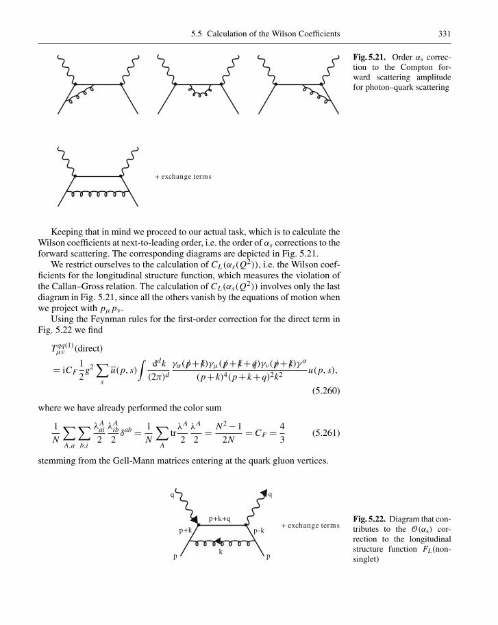
5.5 Calculation of the Wilson Coefficients 331
+ exchange terms
Fig. 5.21. Order αs correc-tion to the Compton for-ward scattering amplitudefor photon–quark scattering
Keeping that in mind we proceed to our actual task, which is to calculate theWilson coefficients at next-to-leading order, i.e. the order of αs corrections to theforward scattering. The corresponding diagrams are depicted in Fig. 5.21.
We restrict ourselves to the calculation of CL(αs(Q2)), i.e. the Wilson coef-ficients for the longitudinal structure function, which measures the violation ofthe Callan–Gross relation. The calculation of CL(αs(Q2)) involves only the lastdiagram in Fig. 5.21, since all the others vanish by the equations of motion whenwe project with pµ pν.
Using the Feynman rules for the first-order correction for the direct term inFig. 5.22 we find
T qq(1)µν (direct)
= iCF1
2g2
∑s
u(p, s)∫
ddk
(2π)dγα(p/+ k/)γµ(p/+ k/+q/)γν(p/+ k/)γα
(p+ k)4(p+ k+q)2k2 u(p, s),
(5.260)
where we have already performed the color sum
1
N
∑A,a
∑b,i
λAai
2
λAib
2δab = 1
N
∑A
trλA
2
λA
2= N2−1
2N= CF = 4
3(5.261)
stemming from the Gell-Mann matrices entering at the quark gluon vertices.
+ exchange terms
q q
p p
p+k p-k
k
p+k+q Fig. 5.22. Diagram that con-tributes to the O(αs) cor-rection to the longitudinalstructure function FL (non-singlet)

332 5. Perturbative QCD I: Deep Inelastic Scattering
In general we have to perform the calculation in d = 4+2ε dimensions toregularize divergencies. However, it turns out that for the projection onto FL theintegral is free of any divergence, which is not the case if we were to project withgµν onto F2.
Performing the projection and using p2 = 0 we obtain
pµ pνT qqµν(direct)= iCF g2 1
2
∑s
∫d4k
(2π)4u(p, s)γαk/p/(k/+q/)p/k/γαu(p, s)
(p+ k)4(p+ k+q)2k2
=−iCF g2∫
d4k
(2π)4tr [k/p/(k/+q/)p/k/p/]
(p+ k)4(p+ k+q)2k2 , (5.262)
where we used∑
s u(p, s)Mu(p, s)= tr[M p/] and γα p/γα =−2p/. The trace canbe further simplified by again using p2 = 0:
tr [k/p/(k/+q/)p/k/p/] = 2k ptr [k/p/(k/+q/)p/]
= (2k p)2tr [(k/+q/)p/]
= 16[(k · p)3+ (k · p)2(p ·q)
]. (5.263)
What remains is therefore to perform the following integral:
pµ pνT qqµν(direct)
=−16iCF g2∫
d4k
(2π)4(k · p)3+ (k · p)2(p ·q)(p+ k)4(p+ k+q)2k2
=−16iCF g2 [Iαβ(p, q)pα pβ p+ (p ·q)Iαβ(p, q)pα pβ]. (5.264)
This will be achieved by using the Feynman parameter technique (4.95). Webegin with the integral
Iαβ(p, q)=∫
d4k
(2π)4kαkβ
(p+ k)4(p+ k+q)2k2
= Γ(4)
Γ(2)Γ(1)Γ(1)
1∫0
du
u∫0
dvu
×∫
d4k
(2π)4kαkβ[
(p+ k)2u+ (p+ k+q)2v+ k2(1−u−v)]4 ,
(5.265)
where we used the Feynman parametrization (see Exercise 4.7) and denote u =1−u, v= 1−v. The denominator can be simplified:[
u(p+ k)2+v(p+ k+q)2+ k2(1−u−v)]4
= k2(1−u−v+u+v)+2k(u p+v(p+q))+ (p+q)2v
= k2+2k(u p+v(p+q))+ (p+q)2v

5.5 Calculation of the Wilson Coefficients 333
= (k+u p+v(p+q))2− (u p+v(p+q))2+ (p+q)2v
= k′2−2vu pq+ (p+q)2vv
= k′2+vv
((p+q)2− u
v2pq
)= k
′2−vvQ2(
1− 2pq(1−u′)Q2
)= k
′2−vvQ2 (1−ωu′)
with u′ = uv
and k′ = k+u p+v(p+q) and therefore
k = k′ − (u′v+v)p−vq . (5.266)
With that we get
Iαβ(p, q)= Γ(4)
1∫0
du
1∫0
dvuv2∫
d4k
(2π)4k′αk′β[
k′2−vvQ2(1−ωu)]4 ,
(5.267)
where we have rewritten the integration
1∫0
du
u∫0
dvu f(u, v)=1∫
0
dv
v∫0
duu f(u, v)=1∫
0
dvv2
1∫0
du′u′ f(u′v, v) .
(5.268)
The fact that the integral will be multiplied by pα pβ again simplifies our cal-culation since due to the onshell condition p2 = 0 we are allowed to retain onlythe terms ∼ qαqβ in the substitution k
′αk′β:
Iαβ(p, q)pα pβ
= Γ(4)(p ·q)21∫
0
dvv2v2
1∫0
duu∫
d4k
(2π)41[
k2−vvQ2(1−ωu)]4 . (5.269)
Similarly we get for the other integral in (5.264)
Iαβ(p, q)pα pβ p
=−Γ(4)(p ·q)31∫
0
dvv2v3
1∫0
duu∫
d4k
(2π)41[
k2−vvQ2(1−ωu)]4 ,
(5.270)

334 5. Perturbative QCD I: Deep Inelastic Scattering
where the only difference is that instead of kαkβ → k′αk′β → v2qαqβ in (5.267)we have kαkβk→−qαqβqv3. The remaining k integration is readily per-formed with the help of the tables in (4.97) to (4.101):∫
d4k
(2π)41[
k2−vvQ2(1−ωu)]4 =
i
(4π)2Γ(2)[
vvQ2(1−ωu)]2
1
Γ(4). (5.271)
Since we simplified the denominator in such an intelligent way that theFeynman parameters factorize, we are now able to perform the
∫dv integration:
1∫0
dvv2v2(vv)−2 = Γ(1)Γ(1)
Γ(2)= 1 ,
1∫0
dvv2v3(vv)−2 = Γ(1)Γ(2)
Γ(3)= 1
2. (5.272)
In passing, we note that the evaluation of the integrals within the Feynmanparameter integral is one of the main obstacles in multiloop calculations.A factorization of Feynman parameters can always be enforced by expand-ing nonfactorized expressions like (u+v)a =∑a
n=0
(an
)unva−n for the price of
introducing an additional sum. Summarizing we get
pµ pνT qq(1)µν (direct)= 16
(4π)2CF g2 (p ·q)3
Q4
1
2
1∫0
duu
(1−ωu)2. (5.273)
The superscript (1) to T qq(1)µν indicates the first order in αs approximation for T qq
µν .To perform the remaining u integration we expand the denominator
1
(1−ωu)2=
∞∑n=0
(n+1)(uω)n (5.274)
and with
1∫0
duunu = Γ(n+1)Γ(2)
Γ(n+3)= 1
(n+2)(n+1)(5.275)
we end up with
pµ pνT qqµν(1)(direct)= 16
(4π)2CF g2 (p ·q)3
Q4
1
2
∞∑n=0
ω2
(n+2)
= CFαs
4π
Q2
x2
∞∑n=0
ωn+1
(n+2). (5.276)

5.5 Calculation of the Wilson Coefficients 335
The crossed diagram doubles even, and cancels odd, powers of ω so that wefind
FqL
2x= 2CF
αs
4π
∑n=2,4,...
4
(n+1)ωn . (5.277)
The nth power of ω corresponds exactly to the nth moment of the structurefunction F2 as we saw in the introductory discussion. Indeed, comparing with(5.256) to (5.259) leads us to the final result
1∫0
dxxn−2 FqL(x, Q2)= CF
αs
4π
4
(n+1)
1∫0
dxxn−2 Fq2 (x, Q2) . (5.278)
Now we want to express the above relation not only on the level of momentsof the structure function but also as a convolution in Bjorken-x space. With
1∫0
dzzn−1z = 1
n+1(5.279)
we can write
1∫0
dxxn−1 Fq2 (x, Q2)= 4CF
αs
4π
1∫0
dzzn−1z
1∫0
dyyn−1 F2( y, Q2)
= 4CFαs
4π
1∫0
dy
1∫0
dz(zy)n−1zF2( y, Q2)
= 4CFαs
4π
1∫0
dy
y
y∫0
dxxn−1(
x
y
)F2( y, Q2)
= 4CFαs
4π
1∫0
dxxn−1
1∫x
dy
y
(x
y
)F2( y, Q2) (5.280)
and therefore
FqL(x, Q2)= 4CF
αs
4π
1∫x
dy
y
(x
y
)Fq
2 ( y, Q2) . (5.281)
So far we have only considered the O(αs) correction coming from photon–quark scattering. However, to O(αs) also diagrams from photon–gluon scatteringcontaining a quark loop contribute (see Fig. 5.23).

336 5. Perturbative QCD I: Deep Inelastic Scattering
+ exchange terms
Fig. 5.23. O(αs) contribu-tion to the Compton forwardscattering amplitude stem-ming from photon–gluonscattering
We will calculate those diagrams that contribute only to singlet structurefunctions in Excercise 5.13. The final result is
FgL(x, Q2)= Tf
( αs
4π
)16
1∫x
dy
y
(x
y
)(1− x
y
)Fg
2 ( y) , (5.282)
where Tf = 12 Nf is the color factor times a factor Nf coming from the sum over
the quark flavors running through the quark loop.For FL we therefore have calculated the complete O(αs) corrections. As can
be seen from (5.280) and (5.282) FL is expressed in terms of the structure func-tion F2(x, Q2) times a factor that is calculable in perturbation theory. F2(x, Q2)
is simply the quark distribution function Fq2 (x, Q2)= xq(x, Q2) and the gluon
distribution function Fg2 (x, Q2)= xG(x, Q2), respectively.
That FL is completely expressed through F2 is due to the fact that only oneset of unpolarized operators Vn(µ
2) contributes to F2 and FL – see (5.175) and(5.176). (One has to keep in mind that the vector operators Vn(µ
2) contributeto the unpolarized structure functions while the axialvector operators An(µ
2)
contribute to the polarized structure functions.)We can therefore express FL and F2 as
1∫0
dxxn−2 FL(x, Q2)= Cn,L
(αs,
Q2
µ2
)Vn(µ
2) ,
1∫0
dxxn−2 F2(x, Q2)= Cn,2
(αs,
Q2
µ2
)Vn(µ
2) , (5.283)
and solving the equations for FL and F2 by eliminating Vn(µ2) we find
1∫0
dxxn−1 FL(x, Q2)=Cn,L
(αs,
Q2
µ2
)Cn,2
(αs,
Q2
µ2
) 1∫0
dxxn−1 F2(x, Q2)

5.5 Calculation of the Wilson Coefficients 337
=∑
m=1 C(m)n,L
(αs4π
)m1∫
0dxxn−1 F2(x, Q2)
(1+∑
m=1 C(m)n,2
(αs4π
)) 1∫0
dxxn−1 F2(x, Q2)
=
C1n,L
αs
4π+[C(2)
n,L −C(1)n,LC(1)
n,2
] ( αs
4π
)2
+O
(( αs
4π
)3)
×1∫
0
dxxn−1 F2(x, Q2) . (5.284)
Here we have written the Wilson coefficients as an expansion in αs/4π andmade use of the fact that FL is equal to zero at zeroth order and that usuallythe corresponding coefficient is normalized to 1 for F2. This means C(0)
n,L = 0
and C(0)n,2 = 1. With this we have shown that to all orders in αs, FL is determined
completely by F2 up to higher-twist(
1Q2
)corrections.
The expansion coefficients C(m)n,2 corresponding to F2 can be calculated in
a similar way as we did for FL . The calculations, however, are more lengthybecause now all diagrams of Fig. 5.21 contribute. An additional complicationarises due to the fact that the calculations have to be carried through in d dimen-sions since for the projection onto F2 the diagrams do not remain finite and haveto be renormalized.
The details of such calculations can be found in the very comprehensive pa-per by Bardeen et al.16 The coefficient functions are available in the literaturefor the first 10 moments up to the third order.17 The coefficient functions for allmoments i.e. the full x dependence are available up to the second order.18 Suchcalculations cannot be done in the simple way presented here for the lowest orderbut depend heavily on the use of algebraic computer codes. Also it seems notto be feasible to push the calculations to even higher orders since at each orderthe number of contributing diagrams increases considerably and with each ad-ditional loop integration the necessary CPU time increases as well. Instead, thestudy of the perturbative series to all orders in certain approximations will be per-sued, e.g. for small n (n characterizes the nth moment of the structure function)or for large Nf .
16 W.A. Bardeen, A.J. Buras, D.W. Duke and T. Muta: Phys. Rev. D 18, 3998 (1978).17 S.A. Larin, P. Nogueira, T. van Ritbergen and J.A.M. Vermaseren: Nucl. Phys. B
492,338 (1997).18 E.B. Zijlstra and W.L. van Neerven: Nucl. Phys. B 383, 525 (1992).

338 5. Perturbative QCD I: Deep Inelastic Scattering
q q
p p
Fig. 5.24. Diagrams con-tributing in O(αs) to thevirtual photon–gluon scat-tering.
EXERCISE
5.13 Calculation of the Gluonic Contribution to FL(x, Q2)
Problem. Calculate in the same way as done in the foregoing text the contribu-tion to FL due to photon–gluon scattering via a quark loop. The correspondingdiagrams are shown in the figure. A usefull trick is to express the product of twopropagators involving an onshell momentum p2 = 0 as
1
(k+ p)21
k2 =1∫
0
du1
(k+u p)4.
Prove this formula and find its generalization.
Solution. The color factor for the diagrams coming from the Gell-Mann matri-ces at the quark–gluon vertices can be written as
1
(N2−1)
∑A
∑B
tr
[λA
2
λB
2
]= 1
(N2−1)
∑A
∑B
1
2δAB = 1
2, (1)
where we summed over outgoing gluon colors and averaged over the incomingones. Together with a factor Nf , which is due to the sum over flavors in the quarkloop, this yields an overall factor Tf = 1
2 Nf .

5.5 Calculation of the Wilson Coefficients 339
We start with the first diagram which we name T (1)ggµν (direct). In the usual
way the exchange term can be found by substituting µ↔ ν and q ↔−q.According to the Feynman rules we write
T (1)ggµν (direct)
= ig2
2Tf
∫d4k
(2π)4tr
[γµ
i
p/+q/+ k/γν
i
p/+ k/γα
i
k/γβ
i
p/+ k/
] (−gαβ), (2)
where we have inserted an additional factor of 12 due to the averaging over the
gluon spin and used(−gαβ
)for the polarization sum 1
2
∑εα(k)εβ(k)=−gαβ/2.
Again we compute i times the time-ordered product. Projecting with pµ pν wefind, with γαk/γα =−2k/,
pµ pνT (1)ggµν (direct)= ig2Tf
∫d4k
(2π)4tr [p/(q/+ k/)p/k/k/k/]
(p+q+ k)2(p+ k)4k2
= 8ig2Tf
∫d4k
(2π)4p · (q+ k)(k p)
(p+q+ k)2(p+ k)4. (3)
The integral can be evaluated in the usual way∫d4k
(2π)4(k+q)αkβ
(p+ k+q)2(p+ k)4
= Γ(3)
Γ(1)Γ(2)
1∫0
duu∫
d4k
(2π)4(k+q)αkβ[
u(p+ k+q)2+u(p+ k)2]3
= Γ(3)
1∫0
duu∫
d4k
(2π)4[k− (p+uq)]α[k− p+uq)]β[
k2−uuQ2]3
=−qαqβΓ(3)
1∫0
duu∫
d4k
(2π)41[
k2−uuQ2]3 +O
(gαβ, pα pβ
)
=−qαqβ
1∫0
duuui
(4π)d2
1(uuQ2
) +O(gαβ, pα pβ
)= −qαqβ
Q2
i
(4π)2· 1
2+O
(gαβ, pα pβ
). (4)
We performed the usual Feynman parametrization (see Exercise 4.7)and wrote the denominator as
[u(p+ k+q)2+u(p+ k)2
]= [(k+ p+uq)2
+ uuq2], where u = 1−u. Inserting this into (3) yields
pµ pνT (1)ggµν (direct)= 4g2Tf
(4π)2(p ·q)2
Q2 . (5)
Exercise 5.13

340 5. Perturbative QCD I: Deep Inelastic Scattering
Exercise 5.13
q
q
p
p
q+k+p
q+kk+p
k
Fig. 5.25. Second type of di-agrams that contribute to vir-tual photon–gluonscattering.
Taking the other four diagrams of the same type into account, i.e. the ex-change term and the opposite direction of the fermion loop, we get a contributionto FL (5.251) of
F(1)gL
2x= 16g2Tf
(4π)2, (6)
which is, however, independent of ω, i.e. proportional to ω0. However, the sumin (5.258) starts as ω2, i.e. after transformation to Bjorken x these four diagramsdo not contribute to the measurable structure function.
The remaining diagrams are sligthly more complicated to evaluate. They areshown in the last row of the figure at the beginnning of this exercise. We writeaccording to the Feynman rules (see Fig. 5.25)
T (1)ggµν (direct)
= 1
2Tfg2i
∫d4k
(2π)4tr
[γµ
i
q/+ k/γα
i
q/+ k/+ p/γν
i
k/+ p/γβ
i
k/
] (−gαβ). (7)
Projecting onto FL we write
pµ pνT (1)ggµν (direct)=− 1
2Tfg2i
×∫
d4k
(2π)4tr [p/(q/+ k/)γα(q/+ k/+ p/)p/(k/+ p/)γαk/]
(q+ k)2(q+ k+ p)2(k+ p)2k2
=+Tfg2i∫
d4k
(2π)4tr [p/(q/+ k/)k/p/(q/+ k/)k/]
(q+ k)2(q+ k+ p)2(k+ p)2k2 ,
(8)
where we used p/2 = p2 = 0 and γαγµγνγγα =−2γγ νγµ. The trace can befurther simplified as
tr [p/(q/+ k/)k/p/(q/+ k/)k/] = 2k · ptr [p/(q/+ k/)(q/+ k/)k/]
− tr [p/(q/+ k/)p/k/(q/+ k/)k/]
= 8(k · p)2(q+ k)2−2p · (q+ k)tr [p/k/(q/+ k/)k/]
= 8(k · p)2(q+ k)2−16p · (q+ k)(k ·q)(p · k)−16p(q+ k)p · k k2+8[p · (q+ k)]2k2 , (9)
so that we get
pµ pνT (1)ggµν (direct)= 8g2iTf [I1(q, p)+ I1(−q, p)
−2I2(q, p)−2I3(q, p)] , (10)

5.5 Calculation of the Wilson Coefficients 341
where
I1(q, p)=∫
d4k
(2π)4(k · p)2
(q+ k+ p)2(k+ p)2k2 ,
I1(−q, p)=∫
d4k
(2π)4(p · (q+ k))2
(q+ k)2(q+ k+ p)2(k+ p)2
=∫
d4k
(2π)4(p · k)2
(k+ p)2(k+ p−q)2k2 ,
I2(q, p)=∫
d4k
(2π)4p · (q+ k)p · k
(q+ k)2(q+ k+ p)2(k+ p)2,
I3(q, p)=∫
d4k
(2π)4p · (q+ k)k ·qp · k
(q+ k)2(q+ k+ p)2(k+ p)2k2 . (11)
The integrals I1(q, p) and I2(q, p) are of the same type as we had before (see(5.265)). Using suitable substitutions we can therefore deduce the correspondingresults directly from the previous calculation of Fq
L . Comparing I1(q, p) with(5.265) we see that (p+ k)2 in the denominator comes now with a power of 1instead of 2. Therefore we copy from (5.269) with evident changes and get
I1(q, p)= (p ·q)2Γ(3)1∫
0
du
1∫0
dvvv2∫
d4k
(2π)41
(k2−vvQ2(1−ωu))3.
(12)
We changed Γ(4)→ Γ(3) corresponding to the different power and weomitted the Feynman parameter (uv), which came from the parametrization of(p+ k)4 in (5.265), which in our case now is (p+ k)2. Also we have taken careof the shift in the integration variable kα→ kα− (uv+v)pα−vqα where due tothe contraction with pα pβ only v2qαqβ contributes.
For the∫
dk integral we get∫d4k
(2π)41[
k2−vvQ2(1−ωu)]3 =
−i
(4π)21
Γ(3)
1
vvQ2(1−ωu). (13)
The∫
dv integration gives
1∫0
dvv2v(vv)−1 = 1
2, (14)
and therefore
I1(q, p)= −i
(4π)2(p ·q)2
Q2 · 1
2
1∫0
du1
(1−ωu). (15)
Exercise 5.13

342 5. Perturbative QCD I: Deep Inelastic Scattering
Exercise 5.13 Expanding
1
1−ωu=
∞∑n=0
(ωu)n , (16)
we find, after trivial integration,
I1(q, p)= −i
(4π)2(p ·q)2
Q2
1
2
∞∑n=0
1
(n+1)ωn . (17)
In the same way we can evaluate I2(q, p):
I2(q, p)=∫
d4k
(2π)4p · (q+ k) p · k
(q+ k)2(q+ k+ p)2(k+ p)2
=∫
d4k
(2π)4(p · k) p · (k−q)
k2(k+ p)2(k+ p−q)2
= Γ(3)
1∫0
du
1∫0
dvv∫
d4k
(2π)4p · (k−vq) p · (k− (1−v)q)[
k2−vvQ2(1+ωu)]3 , (18)
where we again copied from (5.269) and performed in addition to the changescarried out in (12) the substitution q →−q, i.e. ω→−ω. Also the shift of theintegration variable now reads k → k− (uv+v)p+vq.
I2 therefore becomes
I2(q, p)=−Γ(3)(p ·q)21∫
0
du
1∫0
dvv2v
∫d4k
(2π)41[
k2−vvQ2(1+ωu)]3
(19)
= +i
(4π)2(p ·q)2
Q2
1
2
∞∑n=0
1
(n+1)(−ω)n , (20)
where we used (13) and obtained for the∫
dv integration
1∫0
dvv2v(vv)−1 = 1
2. (21)
We also expanded
1
(1+ωu)=
∞∑n=0
(−ωu)n . (22)
Let us now proceed to calculate I3(q, p), which is a little bit more trickysince we deal with four propagators, two of which contain off-shell momenta

5.5 Calculation of the Wilson Coefficients 343
q2 =−Q2 = 0. To circumvent this problem we note the following relation:
1
(k+ p)2A· 1
(k2)B= Γ(A+ B)
Γ(A)Γ(B)
1∫0
duu A−1uB−1
(k+u p)2(A+B), (23)
which holds for arbitrary k2 = 0 and p2 = 0. It can be proven using Feynmanparameters:
1
(k+ p)2A· 1
(k2)B= Γ(A+ B)
Γ(A)Γ(B)
1∫0
duu A−1uB−1[
u(k+ p)2+uk2]A+B
, (24)
where[u(k+ p)2+uk2
]= k2+2ku p = (k+u p)2 completes the proof. Usingthis twice, the integral I3(q, p) can be written as
I3(q, p)=∫
d4k
(2π)4p · (q+ k) k ·q p · k
(q+ k)2(q+ k+ p)2(k+ p)2k2
=1∫
0
du
1∫0
dv∫
d4k
(2π)4p · (q+ k) k ·q p · k
(k+u p)4(q+ k+vp)4
= Γ(4)
1∫0
du
1∫0
dv
1∫0
dyyy
×∫
d4k
(2π)4p · (q+ k) p · k (k−u p) ·q[
yk2+ y(k+q+ (v−u)p)2]4 , (25)
where in the last step k → k−u p is shifted and a third Feynman parameter isintroduced. The denominator can now be simplified in the usual way[
yk2+ y(k+q+ (v−u)p)2]= k2+2k · ( yq+ (v−u)yp)
+ y(q+ (v−u)p)2
=[k+ yq+ (v−u)yp)2+ yy(q+ (v−u)p
]2
= k′2+ yy
[q2+2q · p(v−u)
]= k
′2− yyQ2[1−ω(v−u)] (26)
The shift of the integration momenta k = k′ − yp− (v−u)yp has to beperformed in a similar way in the numerator:
(q+ k)α(k−u p)βkσ[
pαqβ pσ]
= (k′ + yq)α(k′ − yq−vyp−uy p)β(k
′ − yq)σ[
pαqβ pσ]
= k′αk′β(−yq)σ + k′βk′σ (yq)α+ yqα( yq+vyp+uy p)β yqσ[
pαqβ pσ]
= k′2
4(p ·q)2[1−2y]+ yy(p ·q)3(vy+uy)+ yy2(p ·q)2q2 . (27)
Exercise 5.13

344 5. Perturbative QCD I: Deep Inelastic Scattering
Exercise 5.13 Here we used the fact that under integration, contributions like ∼ kα orkαkβkσ vanish and that kαkβ = 1
4 k2gαβ. (See our discussion on dimensionalregularization before.)
With that we are left with two k′ integrations:
1
4
∫d4k′
(2π)4k′2[
k′2− yyQ2(1−ω(v−u))]4
= −i
4(4π)2Γ(3)
Γ(2)Γ(4)
1(yyQ2(1−ω(v−u))
)= −i
2(4π)21
Γ(4)
1(yyQ2(1−ω(v−u))
) (28a)
and∫d4k
(2π)41[
k2− yyQ2(1−ω(v−u))]4
= i
(4π)2Γ(2)
Γ(4)[yyQ2(1−ω)(v−u)
]2 . (28b)
Inserting everything in (25) and performing the trivial∫
dy integration weget
I3(q, p)= i
2(4π)2
1∫0
du
1∫0
dv
(p ·q)3
Q4
(v+u)
[1−ω(v−u)]2
+(p ·q)2Q4 q2 1
[1−ω(v−u)]2
= i
4(4π)2
1∫0
du
1∫0
dv(v+u)ω−2
[1−ω(v−u)]2(p ·q)2
Q2 . (29)
Expanding again in ω yields
1
[1−ω(v−u)]2 =∞∑
n=0
Γ(n+2)
Γ(2)Γ(n+1)(v−u)nωn =
∞∑n=0
(1+n)(v−u)nωn
(30)
and the remaining integrations can be performed:
1∫0
du
1∫0
dv(v−u)n = 1
(1+n)
1∫0
du[(1−u)1+n + (−)nu1+n
]= 1
(1+n)(2+n)
(1+ (−)n) , (31)

5.5 Calculation of the Wilson Coefficients 345
1∫0
du
1∫0
dv(v+u)(v−u)n
=1∫
0
du
[un+2
n+2− (−)n un+2
n+2+2
uun+1
(n+1)− (−)n+1 2un+2
n+1
]
= 1
(n+2)(n+3)− (−)n(n+2)(n+3)
+ 2
(n+2)(n+3)(n+1)
− (−)n+1 2
(n+1)(n+3). (32)
Inserting (30), (31), and (32) into (29) yields
I3(q, p)
=
i
4(4π)2
∞∑n=0
1+n
(n+2)(n+3)
(1− (−)n)+ 2
(n+2)(n+3)
+ 2(−)n(n+3)
ωn+1 − i
2(4π)2
∞∑n=0
1
(2+n)
(1+ (−)n)ωn
(p ·q)2
Q2
=
i
4(4π)2
∞∑n=0
[2
(3+n)− 1
(2+n)
] (1− (−)n)
+2
[1
(2+n)− 1
(3+n)
]+ 2(−)n(n+3)
ωn+1
− i
2(4π)2
∞∑n=0
1
(2+n)
(1+ (−)n)ωn
(p ·q)2
Q2
=
i
4(4π)2
∞∑n=0
1
(2+n)ωn+1 (1+ (−)n)
− i
2(4π)2
∞∑n=0
1
(2+n)
(1+ (−)n)ωn
(p ·q)2
Q2
=⎧⎨⎩ i
2(4π)2
∞∑n=0,2,4,
1
(2+n)ωn+1− i
(4π)2
∞∑n=0,2,4,
1
(2+n)ωn
⎫⎬⎭ (p ·q)2Q2 .
(33)
Taking into account the contribution coming from the exchange term(q →−q), which in this case cancels odd powers of ω and doubles even powers,we find
I3(q, p)+ I3(−q, p)=⎛⎝ −2i
(4π)2
∞∑n=0,2,4,
1
(2+n)ωn
⎞⎠ (p ·q)2Q2 . (34)
Exercise 5.13

346 5. Perturbative QCD I: Deep Inelastic Scattering
Exercise 5.13 To get the final answer we have to insert (34), (17), and (20), into (10), whichyields
pµ pνT (2)ggµν (direct)+ pµ pνT (2)gg
µν (exchange)
= 8g2iTf [2I1(q, p)+2I1(−q, p)−2(I2(q, p)
+I2(−q, p)+ I3(q, p)+ I3(−q, p))]
= 8
(4π)2g2Tf
∑n=0,2,4,
2
(n+1)+ 2
(n+1)− 4
(n+2)
ωn (p ·q)2
Q2
= 32
(4π)2g2Tf
∑n=0,2,4,
1
(1+n)(2+n)ωn
((p ·q)2
Q2
). (35)
Finally we therefore get
F2
2x= 32
αs
4πTf ·
∞∑n=0,2,4,
1
(1+n)(2+n)ωn . (36)
Repeating the steps we did after (5.277), and observing that
1
(1+n)(2+n)= 1
(1+n)− 1
(2+n)=
1∫0
dxxn−1x−1∫
0
dxxn−1x2
=1∫
0
dxxn−1x(1− x) , (37)
the desired result emerges as
FgL(x, Q2)= Tf
( αs
4π
)16
1∫x
dy
y
(x
y
)(1− x
y
)Fg
2 ( y) , (38)
which has been quoted in (5.282).
EXAMPLE
5.14 Calculation of Perturbative Corrections to Structure Functionswith the Cross-Section Method
We have calculated in the previous sections the Wilson coefficients in O(αs)
using operator product expansion and a dispersion relation (the optical theorem),which relates the imaginary part of the forward scattering amplitude to the crosssection. Instead of looking at the imaginary part it is sometimes convenient tocalculate the cross section directly. This procedure is more general and has an

5.5 Calculation of the Wilson Coefficients 347
wider applicablity. We would like to demonstrate this method, which we call thecross-section method, by essentially reproducing the results from the sectionsbefore, i.e. the perturbative corrections to Fq
L and FgL .
Following (5.281) and (5.282), we can denote the structure functionFL(x, Q2) and F2(x, Q2) as
FkL(x, Q2)=
1∫x
dz
zFL,k(z, Q2)Fk
2
( x
z, Q2
), (1a)
Fk2 (x, Q2)=
1∫x
dz
zF2,k(z, Q2)Fk
2
( x
z, Q2
), (1b)
where the index k refers either to quarks q or gluons g. As usual, Q2 =−q2 de-scribes the momentum of the virtual photon. x = Q2/2Pq refers to the Bjorkenvariable with respect to the nucleon state |P 〉. The variable z = Q2/2pq, onthe other hand, corresponds to the Bjorken variable with respect to the partonmomentum p.
At leading order, F(0)k2 is the structure function related to the pure partondensity F(0)q2 = xq(x). FL,k and F2,k describe the radiative corrections to theparton subprocess
k+γ ∗ → X ,
which are illustrated in the Fig. 5.26.In the language of operator product expansion, the distribution functions
xq(x) and xG(x) can be considered as the nonperturbative input parameters,while FL,k and F2,k are the coefficient functions, calculable order by order inperturbation theory. Then FL,k is related to scattering of a longitudially po-larized virtual photon off parton k and F2,k to the scattering of a transverselypolarized photon. Since the variable z corresponds to the Bjorken variable withrespect to the parton momentum, the calligraphic structures F2,k and FL,k canbe interpreted as parton structure functions.
In the following calculation, all problems related to renormalization will beneglected. Indeed, as we have seen before, in the special case we are interestedin, the quantity FL,k(x) is finite at O(αs). In general this function is diver-gent and we have to use a renormalization prescription to remove poles like 1/εthat arise when using dimensional regularization. However, for the projectiononto FL , poles do not arise. Therefore, we can carry out the calculation in d = 4dimensions.
The parton structure functions can be obtained from the parton tensor, whichwe can define as
Wµν = 1
2
1
2π
∑l
∫dPS(l)Mµ(l)M
∗ν (l) (2)
Example 5.14

348 5. Perturbative QCD I: Deep Inelastic Scattering
Example 5.14
X = +
+ ++
+
γ*
k=q,g
Fig. 5.26. Examples of deepinelastic lepton–parton (k+γ ∗ → X) subprocesses
with∫dPS(l) =
⎛⎝ l∏j=1
∫d3 p j
(2π)32p0
⎞⎠ (2π)4δ
⎛⎝p+q−l∑
j=1
p j
⎞⎠=⎛⎝ l∏
j=1
∫d4 p j
(2π)3δ(p2
j)Θ(p0)
⎞⎠ (2π)4δ
⎛⎝p+q−l∑
j=1
p j
⎞⎠ , (3)
and Mµ(l) denotes the amplitude for the photon–parton reaction
γ ∗ + p −→ p1+ p2+· · ·+ pl . (4)
Here p stands for the incoming parton and p1 · · · pl for the partons producedin the scattering reaction. The integral
∫dPS(l) is just the Lorentz invariant
phase space for on-shell particles p2j = 0. Remember that d3 p/(2π)32p0 is the
Lorentz-invariant measure. Note that we have averaged over all spins in the ini-tial state. The parton structure tensor can again be decomposed as in the generalcase in (5.249) in terms of FL and F2
Wµν =(
gµν− qµqνq2
)FL
+(
pµ pν− p ·qq2
(pµqν+ pνqµ
)+ gµν(p ·q)2
q2
)F2
p ·q , (5)

5.5 Calculation of the Wilson Coefficients 349
with the corresponding projection onto FL
FL = Q2
(p ·q)2 pµ pνWµν . (6)
To check wether our normalization is correct we first calculate the zerothorder, i.e. the tree-level contribution which is the first diagram on the right-handside of the pictorial equation in Fig. 5.26, i.e. the contribution without additionalgluons.
Inserting the tree-level amplitude
Mµ(1)= u(p, s)γµu(p1, s1) (7)
into (2) yields
Wµν = 1
4π
∫d4 p1
(2π)3δ(p2
1)Θ(p0)(2π)4δ(p+q− p1)tr
[γµ p/γν p/1
].
When projecting onto F2 with −gµν/2 (see (5.252); the pµ pν term of theprojector does not contribute!) we get
−gµν
2Wµν = 1
2δ((p+q)2
)Θ(p0)4p ·q
= δ
(Q2
z(1− z)
)Q2
z= δ(1− z)= F2(z) , (8)
where we have used p2 = 0 and 2p ·q/Q2 = 1/z. This result has an obvious in-terpretation and – if inserted into (1) – shows that at zeroth order the structurefunction is equal to the bare parton density
Fq2 (x)= F(0)q2 (x)= xq(x) , (9)
as it must be. To obtain the corresponding first-order corrections to FL we haveto analyze the diagrams shown in Fig. 5.27.
This requires the evaluation of the real-gluon emission graphs (c) and (d)and also the interference of the lowest-order graph (a) with the virtual gluonexchange graph (b). Due to the equations of motion
p/u(p)= u(p)p/= 0 , (10)
only diagram (c) contributes to FL . All other diagrams vanish under the projec-tion (6). The real gluon emission graphs describe the reaction
γ ∗(q)+q(p)−→ q(p′)+G(k) ,
where the symbols in brackets are the momenta carried by the correspondingparticles.
Note that the letter q in γ ∗(q) denotes the four-momentum of the pho-ton while q(p) denotes a quark with four-momentum p. To calculate the crosssection we must evaluate the two-particle phase space
Example 5.14

350 5. Perturbative QCD I: Deep Inelastic Scattering
Example 5.14
+
+
a) b)
c) d)
Fig. 5.27. Diagrams giv-ing the correction of orderO(αs) to the pointlike quark–photon cross section. Theinterference term of |a+b|2give rise to a contribution oforder O(αs). For FL with theprojection pµ pν and p2 = 0only diagram (c) gives anonzero contribution
∫dPS(2) =
∫d4 p′
(2π)3
∫d4k
(2π)3(2π)4δ(p+q− p′ − k)δ+(p
′2)δ+(k2) ,
(11)
where we introduced the shorthand notation δ+(p2)= δ(p2)Θ(p0).We will work in the centre-of-mass system (CMS) of the parton and vir-
tual photon. The incoming momenta are directed along the z direction. Thus thekinematics is given by
p = (|p|, 0, 0, |p|) ,q = (q0, 0, 0,−|p|)=
(√|p|2−Q2, 0, 0,−|p|
). (12)
The momenta of the produced particles are denoted as
k = (|k|, 0, |k|sinΘ, |k|cosΘ) ,
p′ = (|k|, 0,−|k|sinΘ,−|k|cosΘ) , (13)
so that k+ p ′ = 0 and k2 = p′2 = 0. For later use we will also introduce theMandelstam variables
s = (p+q)2 , t = (p− k)2 , u = (p− p′)2 . (14)
The phase space then can be written as∫dPS(2) =
∫d4k
(2π)2δ+(k2)δ+
((p+q− k)2
)

5.5 Calculation of the Wilson Coefficients 351
=∫
d4k
(2π)2δ+(k2)δ+(s−2|k|√s)
=∫
d3k
(2π)2(2|k|)δ+(s−2|k|√s) , (15)
where∫dk0δ+(k2)=
∫dk0δ(k02−|k|2)Θ(k0)= 1
2|k| =1
2|k| . (16)
has been used. Performing the trivial φ integration yields
∫dPS(2) = 1
4π
∞∫0
d|k| |k|1∫
−1
d cosΘδ(s−2√
s|k|) . (17)
To proceed, let us introduce the variable y = 12(1+ cosΘ) and write the
δ function as
δ(s−2√
s|k|)= 1
2√
sδ
(|k|− 1
2
√s
)(18)
so that the simple expression
∫dPS(2) = 1
8π
1∫0
dy (19)
is obtained. Now we write the Mandelstam variables s, t, u (14) in terms of thevariables Q2, y, and z = Q2/2p ·q and find
s = Q2
z(1− z) ,
t = −Q2
z(1− y) ,
u = −Q2
zy . (20)
The last two equations are obtained by recognizing that in the CMS
t = (p− k)2 =−2p · k =−2|p||k|(1− cosΘ)=−p ·q(1− cosΘ)
= −Q2
z(1− y) ,
u = (p− p′)2 =−2p · p′ = −2|p||k|(1+ cosΘ)=−p ·q(1+ cosΘ)
= −Q2
zy , (21)
Example 5.14

352 5. Perturbative QCD I: Deep Inelastic Scattering
Example 5.14 with z = Q2/2p ·q. Twice we have used here that in the CMS
p ·q = p0q0− pq = |p|q0+|p||p| = |p|(
q0+ p0)= |p|(2|k|) . (22)
With these preliminaries we have everything at hand to calculate the realgluon emission process. For the amplitude in (c) of the last figure we write
Mµ = gua(p′, s′)γµi
p/− k/γαλA
ab
2ub(p, s)ε∗α , (23)
so that we get for the spin-summed matrix element∑s′,s,ε
Mµ(2)M∗ν (2)
= g2CF
∑s′,s,ε
u(p′, s′)γµ1
p/− k/γαu(p, s)u(p, s)γβ
1
p/− k/γνu(p′, s′)ε∗αεβ
= g2CF tr
[p/′γµ(p/− k/)γα p/γβ(p/− k/)γν
] (−gαβ)
(p− k)4(24)
where the color factor is
1
N
∑a,b
∑A,B
λAab
2
λBba
2δAB = N2−1
2N= CF = 4
3(25)
and the sum over gluon polarisation in the Feynman gauge∑ε
ε∗αεβ =−gαβ . (26)
Projecting onto FL with pµ pν we find
pµ pν∑spins
Mµ(2)M∗ν (2)=
g2CF
(p− k)4·2 tr
[p/′ p/k/p/k/p/
]= g2CF
(p− k)4·8(p · k)2 tr
[p/′ p/
]= −4g2CF
(p− k)4(−2p · k)2(−2p′ · p)
= −4g2CF
z2 z2u =−4g2CFu =+4g2CFQ2
zy .
(27)
In the last step we inserted the Mandelstam variables according to (20).Inserting (27) and (19) into (2) yields
pµ pνWµν = 1
8π2 g2CFQ2
z
1∫0
dyy
= 1
16π2 g2CFQ2
z. (28)

5.5 Calculation of the Wilson Coefficients 353
Using (6)
FL = Q2
(pq)2pµ pνWµν = 4z2
Q2 pµ pνWµν (29)
gives
FL = g2
4π2 CF · z = 4CFαs
4π· z , (30)
and inserting that into (1) brings us finally to
FqL(x, Q2)= 4CF
αs
4π
1∫x
dz
zzFq0
2
( x
z, Q2
)
= 4CFαs
4π
1∫x
dy
y
(x
y
)Fq0
2
(y, Q2
). (31)
This confirms by use of a completely different method our former result of(5.281). The confirmation of the gluon contribution Fg
L will be left to Excer-cise 5.14.
Here we have presented a calculation of the αs correction to FL which ap-parently is much simpler than the more formal calculation we did before. Also itmight appeal to the physical intuition to calculate directly the cross section andstay as close as possible to the parton model in each step of the calculation.
The calculations of the corrections to F2 may be found in the work ofG. Altarelli at al.19 The complete 2-loop corrections were calculated by Zijlstraand van Neerven.20 However, the cross-section method becomes increasinglydifficult with 3-particle phase space integrals and, at least in the near future,calculations of 3-loop corrections do not seem to be feasible.
Finally, it is worthwhile to mention that 3-loop corrections are already avail-able for the first 10 moments of FL and F2 with the operator product expansionmethod.21
19 G. Altarelli, R.K. Ellis, G. Martinelli: Nucl. Phys. B 157, 461 (1979).20 E.B. Zijlstra and W.L. van Neerven: Nucl. Phys. B 383, 525 (1992) 525.21 S.A. Larin, P. Nogueira, T. van Ritbergen and J.A.M. Vermaseren:
Nucl. Phys. B 492, 338 (1997).
Example 5.14

354 5. Perturbative QCD I: Deep Inelastic Scattering
pp
k k
p' p '
+Fig. 5.28. Diagrams con-tributing to order αs tophoton–gluon scattering. Thewavy line represents the vir-tual photon, the curled linethe gluon
EXERCISE
5.15 Calculation of the Gluonic Contribution to FLwith the Cross-Section Method
Problem. Calculate the contribution of photon–gluon scattering to the lon-gitudinal structure function. Use the cross-section method as in the previousexample 5.14.
Solution. The necessary diagrams we encounter are shown in the Fig. 5.28.Let us first collect the necessary definitions from Examples 5.13 and 5.14.
The gluonic structure function is given by a convolution
FgL =
1∫x
dz
zFL(z, Q2)F(0)g2
( x
z, Q2
)(1)
with a function FL(z, Q2) calculable in perturbation theory and the gluon dens-ity F(0)g2 (x, Q2)= xG(x, Q2). We calculate FL by projecting onto the partonicscattering tensor Wµν (see (6) and (29) of Example 5.14):
FL(z, Q2)= 4z2
Q2 pµ pνWµν , (2)
where the partonic scattering tensor to the order we are working is given by
Wµν = 1
(4π)
1
(8π)
1∫0
dyMµ(2)M∗ν (2) , (3)
where we have used the representation (2) and (19) from Example 5.14 for thetwo-particle phase space (l = 2). The kinematics are the same as previously; i.e.for the reaction
g(p)+γ ∗(p)→ q(k)+q(p′) (4)
we choose
p = (|p|, 0, 0, |p|) ,k = (|k|, 0, |k| sin θ, |k| cosΘ) ,
p′ = (|k|, 0,−|k| sin θ,−|k| cosΘ) , (5)

5.5 Calculation of the Wilson Coefficients 355
and define the Mandelstam variables as
s = (p+q)2 = Q2
z(1− z) ,
t = (p− k)2 = −Q2
z(1− y) ,
u = (p− p′)2 = −Q2
zy , (6)
with y = 12 (1+ cosΘ). Remember also that p′2 = p2 = 0 = k2, q2 =−Q2 and
that the Bjorken variable with respect to the parton momentum p is definedas z = Q2/2p ·q. With these definitions the calculation is straightforward. Theamplitude of the process reads
Mµ(2)= g
[ua(p′)γµ
i
p/− k/
λAab
2γαub(k)
+uα(p′)γαλA
ab
2
i
q/− k/γµub(k)
]· εα . (7)
When squaring we find for the color sum
1
N2−1
∑A,B,a,b
λAab
2
λAba
2= 1
N2−1
∑A,B
trλA
2
λA
2= 1
N2−1
∑A,B
1
2δAB = 1
2.
(8)
Together with the sum over quark flavors this gives a factor Tf = 12 Nf . With
p′ − p = q− k the squared amplitude becomes
pµ pν∑spins
Mµ(2)M∗ν (2)
=Tfg2
tr[
p/(p/− k/)γαk/γβ(p/− k/)p/p/′] · 1
(p− k)4
+ tr[γα(p/′ − p/)p/k/p/(p/′ − p/)γβ p/′
] · 1
(p− p′)4(9)
+ tr[
p/(p/− k/)γαk/p/(p/′ − p/)γβ p/′] 1
(p− p′)2(p− k)2
+tr[γα(p/′ − p/)p/k/γβ(p/− k/)p/p/′
] 1
(p− p′)2(p− k)2
(−gαβ)
= Tfg22
tr[
p/k/k/k/p/p/′] · 1
t2 tr[
p/′k/p/p/′ p/′] · 1
u2
− tr[
p/k/p/′ p/k/p/′] · 1
ut− tr
[k/p/p/′k/p/p/′
] · 1
ut
. (10)
Exercise 5.15

356 5. Perturbative QCD I: Deep Inelastic Scattering
Exercise 5.15 The first two traces vanish due to k2 = p′2 = 0 and the second two are identicalbecause tr
(γαγβ . . . γγσ
)= tr(γσγ . . . γβγα
). The remaining two traces give
−tr[
p/k/p/′ p/k/p/′]= tr
[p/k/p/′k/p/p/′
]= (2p · p′)(2p′ · k) · tr [p/k/]
= 2u · t(2p′ · k)= 2u · t · s . (11)
What remains is therefore
pµ pν∑spins
Mµ(2)M∗ν (2)= Tfg2 ·8s = 8
Q2
z(1− z)Tf g2 . (12)
Inserting this into (2) we finally find
FL(x, Q2)= g2
πTfz(1− z)
= 16( αs
4π
)Tfz(1− z) , (13)
which inserted into (1) gives the final answer
FgL(x, Q2)= 16
( αs
4π
)Tf
1∫x
dz
z[z(1− z)] F(0)g2
( x
z, Q2
)
= 16( αs
4π
)Tf
1∫x
dy
y
(x
y
(1− x
y
))F(0)g2 ( y, Q2) , (14)
which is completely in agreement with our previous result in (5.282).
5.6 The Spin-Dependent Structure Functions
In recent years it has become possible to measure, in addition to the struc-ture functions F1(x, Q2) and F2(x, Q2), the so-called spin-dependent structurefunctions g1(x, Q2) and g2(x, Q2). The spin-dependent structure functions playa role only when the scattered leptons and hadrons are polarized. The origin ofthese additional structure functions is quite obvious. For a polarized hadron, e.g.,a proton, there is an additional Lorentz vector available, namely the spin vec-tor sµ. Accordingly (3.6) has to be extended by some additional terms. Repeatingthe analysis of Chap. 3 with the additional spin vector, we are led to the following

5.6 The Spin-Dependent Structure Functions 357
form of the scattering tensor:
Wµν =(−gµν+ qµqν
q2
)W1(x, Q2)
+(
Pµ−qµq · P
q2
)(Pν−qν
q · P
q2
)W2(x, Q2)
M2
+ iεµνλσqλsσ MG1(x, Q2)
+ iεµνλσqλ(sσq · P− Pσq · s)G2(x, Q2)
M. (5.285)
This equation is obviously an extension of (3.18). The factor i guarantees thatthe transition current is real (the relation Γ ∗
µ(p ↔ p′)= Γµ must hold; see Ex-ercise 3.3), while the ε tensor ensures that qµWµν = qνWµν = 0 holds. Sincethe additional contributions change their sign when the hadron spin direction isreversed, they cancel upon spin-averaging. Thus only spin-independent struc-ture functions can be measured with an unpolarized target. Analogously to theunpolarized case, dimensionless functions are introduced according to
MG1(x, Q2)= g1(x, Q2)
P ·q ,G2(x, Q2)
M= g2(x, Q2)
(P ·q)2 . (5.286)
This choice is motivated by the fact that g1 has a simple interpretation in termsof parton distributions and g2(x) thus occurs on the same footing as g1(x). Theadditional spin-dependent contributions to the hadron scattering tensor are an-tisymmetric; thus they cannot contribute when contracted with the symmetric,unpolarized lepton tensor of (3.20). In order to measure polarized structure func-tions in deep inelastic scattering, the lepton must also be polarized. The resultingleptonic scattering tensor is
Lµν = 1
4tr[(p/+m)(1− s/eγ5)γµ(p/′ +m)γν]
= 1
4[pµ p′ν+ pν p′µ− gµν(p · p′ −m2)]
− m
4tr(p/s/eγ5γµγν)− m
4tr(s/eγ5γµ p/′γν)
= 1
4[pµ p′ν+ pν p′µ− gµν(p · p′ −m2)]+ imεµναβqαsβe , (5.287)
where 12(1− s/γ5) is the standard spin projection operator, and sβe the spin vector
of the electron. Thus the polarized lepton tensor also contains an antisymmetricpart. Contracting both, we obtain the additional term
LµνWµν = · · ·−2mM(gλαgσβ− gλβgσα)qλsσp qαsβe G1
− m
M(gλαgσβ− gλβgσα)q
λ(q · Psσp −q · sp Pσ )qαsβe G2 . (5.288)
This poses the question of what choice of the polarization of electron and hadron,i.e., nucleon, is most suitable. The relevant vectors in the centre-of-momentum

358 5. Perturbative QCD I: Deep Inelastic Scattering
frame are
pµ = (Ee, 0, 0, pe) , Pµ = (Ep, 0, 0,−Pp)
sµe (longitudinal)=±(pe, 0, 0, Ee) · 1
m,
sµp (longitudinal)=±(pp, 0, 0,−Ep) · 1
M,
sµe (transverse)=±(0, 1, 0, 0) and ± (0, 0, 1, 0) ,
sµp (transverse)=±(0, 1, 0, 0) and ± (0, 0, 1, 0) . (5.289)
We recognize that the following products are large:
se(l) · sp(l)≈±2Ee Ep
mM, se(l) · P ≈±2
Ee Ep
m. (5.290)
All the other scalar products in (5.288) are considerably smaller. Thus to meas-ure spin-dependent structure functions, longitudinally polarized leptons must bescattered off longitudinally or transversely polarized nucleons. This property canalso be seen from projecting on physical degrees of freedom of the photon in-stead of summing over photon polarizations. In this case, the hadronic scatteringtensor is contracted with ε∗µεν. Here ε is the polarization vector of the virtual pho-ton. In order for spin-dependent terms to be able to contribute, this expressionmust contain an antisymmetric part. As can easily be checked, this is the caseonly for longitudinal polarization vectors, e.g., it holds for
εµ = (0, 1, i, 0)/√
2 that ε∗1ε2 =−ε∗2ε1 . (5.291)
A longitudinally polarized photon is most readily emitted by a longitudinallypolarized lepton. For other lepton polarizations its coupling is suppressed byexactly the kinematic factors of (5.288).
In the experiments performed up to now, a longitudinally polarized protontarget has been used, and the asymmetry
A =[
d2σdE′ dΩ(↑↑)− d2σ
dE′ dΩ(↑↓)]
[d2σ
dE′ dΩ(↑↑)+ d2σdE′ dΩ(↑↓)
] (5.292)
has been measured.Inserting (5.289) into (5.288) one finds, for longitudinal polarization,
A1 = D
g1(x)− 2Mx
Ey g2(x)
F1(x)+η
√2Mx
Ey
g1(x)+ g2(x)
F1(x)
, (5.293)

5.6 The Spin-Dependent Structure Functions 359
with
D = y(2− y)
y2+2(1− y)(1+ R),
y = E− E′
E, R = σγ ∗L
σγ ∗T,
η= 2γ(1− y)
2− y, and γ =
√Q2M 2
ν2 =√
2Mx
Ey. (5.294)
For transverse proton polarization the resulting asymmetry reads
A2 =[
d2σdE′ dΩ(↑→)− d2σ
dE′ dΩ(↓→)]
[d2σ
dE′ dΩ(↑→)+ d2σdE′ dΩ(↓→)
]= D
√2ε
1+ε
(√2Mx
Ey
g1(x)+ g2(x)
F1(x)−η1+ε
2ε
g1(x)− 2MxEy g2(x)
F1(x)
)
−→√
2Mx
E− E′g1(x)+ g2(x)
F1(x)for Q2 →∞, y → 1 (5.295)
with ε= (1− y)/(1− y+ y2/2). Since the cross sections for transverse and lon-gitudinal polarization should be of approximately the same size, we deduce thatg2(x) is certainly not larger than g1(x). Therefore the contribution of g2(x) atlongitudinal polarization is suppressed by a factor Mx/E and constitutes onlya small correction. The asymmetry A2 therefore measures mainly the ratio ofg1(x) to the unpolarized structure function F1(x). Next, there is the questionof whether g1(x) can be given a practical meaning like F1(x)? This is indeedthe case. To see this, it is sufficient to compare the hadronic and the leptonicscattering tensor of (5.285) and (5.287), respectively.
Obviously each Dirac particle gives a contribution with the same form as thatproportional to G1 multiplied by the probability to find a quark with the fittingmomentum fraction x and the right polarization. Accordingly, one obtains, inanalogy with the parton interpretation of F1,
F1(x)= 1
2
∑q=u,d,u,d...
q(x)Q2q , (5.296)
where q(x) is the probability of finding a quark q with momentum fraction x,a similar expression for g1(x)
g1(x)= 1
2
∑q=u,d,u,d...
Q2q
[q↑(x)−q↓(x)
]. (5.297)
Here q↑(x) indicates the probability of finding a quark with a momentum frac-tion x polarized in the same direction as the whole proton. The asymmetry

360 5. Perturbative QCD I: Deep Inelastic Scattering
Fig. 5.29. The relationshipbetween deep inelastic scat-tering and the forward ma-trix element
measured is a measure of the distribution of the proton spin among its con-stituents.
One of the most important properties of unpolarized structure functions isthat the momentum fraction deduced from them, which is carried by the quarks,accounts for only half of the total momentum. This is striking evidence for theexistence of gluons. Analogously, from polarized structure functions we can askhow much of the proton spin is carried by quarks, how much by gluons and howmuch is present in angular momentum. This question has, up to now, not beenuniquely answered. The present experimental data have caused strong theoret-ical discussions and led to the design of much improved and completely newexperiments. In the near future, experiments of the type
e↑(long.)+p↑, 3He↑, d↑(long. or trans.)→ e′ + X ,
e↑(long.)+p↑, 3He↑, d↑(long. or trans.)→ e′ +π±+ X ,
p+p↑(trans.)→ γ + X plus many more channels (5.298)
should be performed. In addition, polarized proton–proton collisions area possibility for the future.
This field is extremely active right now and a more detailed discussion ofthe current situation is not suitable for a textbook. Instead, we consider two par-ticular aspects where crucial concepts of QCD can be exemplified. As it turnsout, nearly all techniques of QCD are, in a nearly singular manner, important inanalyzing spin structure.
In particular, we consider the following aspects of the discussion.
1. The Bjorken and Ellis–Jaffe sum rule: From the knowledge of the axial vec-tor coupling in weak interactions, predictions based on isospin and SU(3) flavorsymmetry for
∫dx(gp
1 (x)− gn1 (x)) and
∫dxgp
1 (x) can be obtained. This isa nice example that flavor symmetry continues to play an important role evenafter the introduction of color SU(3).
2. The axial anomaly and the gluonic contribution to g1(x): The axial anomalyplays a major role for hadronic physics in general. We met it in Sect. 4.2 when re-viewing the foundations of QCD and will show in Exercise 7.2 its importance inunderstanding lattice QCD. As it turns out, the anomaly can contribute to the spinstructure function in a subtle manner. The analysis of this effect gives exquisiteinsight into the physical meaning of the anomaly.

5.6 The Spin-Dependent Structure Functions 361
Let us start by discussing the Bjorken sum rule. The antisymmetric (spin-dependent) part of the hadronic scattering tensor can be written as an axial-vectorforward matrix element of the proton (see Fig. 5.29). As the proton couplesto quarks we find that the spin-asymmetric part of the cross section ∆σ isproportional to
iγµ p/′γν εµναβ = p′σ(gµσ γν+ gσν γµ− gµν γσ + iεµσνλ γ
λ γ5)
i εµναβ
= p′σ εµνσλ εµναβ γλ γ5
=−2p′σ(g ασ g β
λ − g βσ g α
λ
)γλ γ5
=−2p′α γβ γ5+2p′β γα γ5 , (5.299)
where we have used the well-known decomposition of the product of threegamma matrices. Thus we find that
∆σ ∼∑
q
⟨p s
∣∣ Q2qq γα γ5 q
∣∣ p s⟩. (5.300)
It is important to note that, owing to the optical theorem, we have obtaineda forward cross section, i.e., the momentum transfer is zero. In contrast, themomentum transfer in the lepton–hadron scattering reaction qµ is very large,but squaring this diagram to obtain the cross section leads to a graph in whichthe second photon removes the momentum transferred by the first. (This is justa description of the content of the optical theorem.) Thus this forward matrixelement can be related by isospin symmetry to a corresponding matrix elementbetween neutron and proton. More precisely we write
Q2 = 15
18+ 1
3τ3 =
49 for the up quark19 for the down quark
, (5.301)
implying that
∆σp−∆σn ∼ 1
3
⟨N s
∣∣τ3 q γα γ5 q∣∣N s
⟩, (5.302)
where N= (pn
)is the usual nucleon doublet. Now we can introduce τ+τ−+
τ−τ+ = 11; we obtain
∆σp−∆σn ∼ 1
3
⟨N s
∣∣∣(τ+τ−+ τ−τ+) τ3 q γα γ5 q∣∣∣N s
⟩= 1
3
⟨N s
∣∣∣(τ+τ−− τ−τ+)q γα γ5 q∣∣∣N s
⟩= 1
3
⟨p s
∣∣τ+ q γα γ5 q∣∣n s
⟩ + h.c. . (5.303)
This, however, is just the weak-interaction matrix element of neutron beta decay.The corresponding coupling is just gA/gV . Putting all the constants together, weend up with
1∫0
dx[gp
1 (x)− gn1 (x)
]= 1
6
gA
gV. (5.304)

362 5. Perturbative QCD I: Deep Inelastic Scattering
This is the famous Bjorken sum rule, which allows us to connect the proton andthe neutron results. It is strictly valid for Q2 →∞. Various perturbative andhigher-twist corrections have been calculated:
1∫0
dx[gp
1 (x, Q2)− gn1 (x, Q2)
]= 1
6
gA
gV
[1− αs
π− 43
12
(αs
π
)2]
+ M2
Q2
1∫0
dx x2[
2
9
(gp
1 − gn1
)(x, Q2)+ 4
3
(gp
2− gn2
)(x, Q2)
]
+ 4
9
M2
Q2 ( f2u− f2d)+ 4
9
M2
Q2 (d2u−d2d) (5.305)
with
2(M2)2 f2qsσ = ⟨P S
∣∣g q Gσλ γλ q∣∣P S
⟩, q = u, d . (5.306)
The matrix element d2 is defined in Example 5.16. The f2q can be calcu-lated, for example, by QCD sum rule techniques and turn out to be small.Also the d2q have been estimated and they are expected to give measurablecontributions.22 The mass correction is small, basically because of the factor x2
which suppresses the small x contributions.Thus the Q2 dependence of the Bjorken sum rule is well under control. It is
especially noteworthy that no anomalous dimension, i.e., no factor of the form[α(Q2) / α(Q2
0)]−d/2b, occurs on the right-hand side of (5.305). This fact hasa simple physical reason. The main part of the Q2 evolution of unpolarized struc-ture functions is due to the many quark–antiquark pairs that contribute at highQ2 (see Fig. 5.23). Because the vector coupling to gluons conserves helicity,these quark pairs are, however, predominantly unpolarized. In fact a double spinflip is needed to obtain a polarized qq pair, and except for very small values ofx this is completely suppressed. Consequently the zeroth moment of gp
1 , gn1 ,
gp2, gn
2 should show only a very mild Q2 dependence. (Actually there is goodreason to believe that
∫g2(x) dx ≡ 0.) Now, assuming that the strange quarks
are unpolarized, which is actually a very controversal assumption, we can ob-tain the Ellis–Jaffe sum rule from (5.305). From the definition of g1(x) we have,assuming strict isospin symmetry at the quark level, which is also controversial,
1∫0
dx gp1 (x)=
1
2
(4
9∆u+ 1
9∆d
),
22 E. Stein, P. Gornicki, L. Mankiewicz, A. Schäfer and W. Greiner, Phys. Lett. B 343,369 (1995).

5.6 The Spin-Dependent Structure Functions 363
1∫0
dx gn1 (x)=
1
2
(4
9∆d+ 1
9∆u
), (5.307)
where ∆u, ∆d are the fractions of the proton spin carried by the u and d quarks,respectively.
The Bjorken sum rule (5.304) implies that
1∫0
dx gp1 (x)−
1∫0
dx gn1 (x)=
1
6
(∆u−∆d
)= 1
6
gA
gV,
∆u =∆d+ gA
gV, (5.308)
which is already one constraint. Still another constraint comes from the coup-ling of s and u quarks in hyperon decays. To understand this we have to reviewa little group theory. The general axial vectorial flavor SU(3) matrix element〈B|S5
jσ |B′ 〉 can be analyzed with the equivalent of the Wigner–Eckhardt theo-rem. Here B, B′ are baryon states from the flavor octet, σ is the Lorentz index,and j = 1, . . . , 8 is the index of the SU(3) generator. We find that
〈p | S5jσ | p 〉 = c ·nσ
⎡⎣⎛⎝ 8 8I = 1
2 I3 =−12 I = 1
2 I3 = 12
Y =−1 Y = 1
∣∣∣∣∣∣81
I j − I3 j−Y j
⎞⎠ A1
+⎛⎝ 8 8
I = 12 I3 =−1
2 I = 12 I3 = 1
2Y =−1 Y = 1
∣∣∣∣∣∣82
I j − I3 j−Y j
⎞⎠ A2
⎤⎦×⎛⎝ 8 8
I j − I3 j I j I3 j−Y− j Y j
∣∣∣∣∣∣ 10
⎞⎠ . (5.309)
The isoscalar factors are listed.23 A peculiarity of the SU(3) group is the appear-ance of two unequivalent octet representations. This is related to the fact thatthree octets can be coupled either by the symmetric dabc or the antisymmetricfabc structure constants. It leads to the definition of two constants, D and F:
⟨N∣∣S5
3σ
∣∣N ⟩= c ·nσ(√
30
40A1+
√6
24A2
)=: c ·nσ
(D+ F
),
D =√
30
40A1 , F =
√6
24A2 . (5.310)
Every axial-vector matrix element coupling two baryon states from the octet isthus proportional to a specific combination of D and F and can therefore be used
23 See J.J. de Swart: Rev. Mod. Phys. 35 (1963) 916.

364 5. Perturbative QCD I: Deep Inelastic Scattering
Fig. 5.30. Graphs contribut-ing to the Q2 dependenceof the zeroth moment ofthe unpolarized structurefunctions. For the spin-dependent structure func-tions only (b) contributes,since the quark–antiquarkpairs produced are unpolar-ized
to measure F/D. However, the combined analysis of all the hyperon decays de-scribed by different groups gave conflicting results. A conservative estimate isF/D = 0.55–0.60. From (5.310) we read off
∆u−∆d = F+D . (5.311)
Similarly by inserting the SU(3) isoscalar factors we get⟨N∣∣S5
8σ
∣∣N ⟩= c ·nσ(− 1
4√
10A1+
√2
8A2
)= c ·nσ
(− 1√
3D+√3F
)(5.312)
⇒ 1√3
(∆u+∆d−2∆s
)=√3F− 1√
3D . (5.313)
Assuming again that ∆s= 0 we obtain another independent combination,
∆u+∆d
∆u−∆d= 3F−D
F+D= 3F/D−1
F/D+1, (5.314)
which together with (5.309) allows us to determine1∫
0gp
1 (x) dx. A complete
analysis along these lines gives
1∫0
dx gp1 (x, Q2)= gA
gV
[1
18
3F/D+1
F/D+1
(1− αs
π
)+ 1
9
3F/D−1
F/D+1
(1− αs
π
)]
+ M2
Q2
1∫0
dx x2[
2
9gp
1 (x, Q2)+ 4
3gp
2(x, Q2)
]
− 4
9
1
Q2
(4
9f2u+ 1
9f2d+ 1
9f2s
)≈ 0.172±0.009 for Q2 = 5 GeV2 . (5.315)
This is the Ellis–Jaffe sum rule. As mentioned several times already, its validity isa matter of dispute. We have presented it here to illustrate the potential usefulnessof flavor SU(3) for the analysis of deep inelastic scattering cross sections.

5.6 The Spin-Dependent Structure Functions 365
Fig. 5.31. The perturbativeanomalous gluon contribu-tion to g1
Next let us discuss the role of the anomaly for the isosinglet axial-vectorcurrent. To illustrate the point consider first the perturbative graph in Fig. 5.31.
It is obvious that for Q2 →∞ one indeed obtains the triangle anomaly, im-plying pointlike photon–gluon coupling. The basic problem of this interpretationis also obvious from Fig. 5.29, namely that there is no unambiguous way to sepa-rate the quark contribution and the anomalous gluonic contribution. It is unclearwhether the quarks of the fermion line should be absorbed into ∆u, ∆d, etc. orinto a contribution of the structure
∆gp1 (x)=
⟨Q2
q
2
⟩ 1∫0
dz
zA( x
z
)∆G(z) . (5.316)
In other words, the∆qs appearing in the analysis we have presented so far shouldbe split up according to
∆q =∆q− αs
2π∆G · c . (5.317)
It turns out that, for variety reasons, such a separation is very problematic.
1. Performing the perturbative calculation for the graph in Fig. 5.29 we get con-stants c that depend critically on the chosen infrared regulators indicating thatwe are not looking at an infrared safe quantity.
2. From the operator-product-expansion point of view, we find that there is nogauge-independent local definition of ∆G.
3. A so-called large gauge transformation, i.e., a gauge transformation witha nonzero topological quantum number, shifts contributions from ∆q to ∆G.A detailed discussion of this rather complicated issue is beyond the frameworkof this book.
On the other hand, there exists a practical argument for the decomposition(5.317). If we construct a phenomenological model for∆q, we will most proba-bly miss the highly virtual quark components from Fig. 5.29. Therefore it mightbe easier to model ∆q and ∆G instead.
We will not discuss these still very much disputed questions further.

366 5. Perturbative QCD I: Deep Inelastic Scattering
EXAMPLE
5.16 Higher Twist in Deep Inelastic Scattering
In the framework of operator product expansion we found that structure func-tions can be represented as
1∫0
dxxn−2 F(x, Q2)= Cn(αs, Q2/µ2)Vn(µ2)+O(1/Q2) , (1)
where Vn(µ2) are the reduced matrix elements of the twist-2 operators (see
(5.257)–(5.259)). The Wilson coefficients Cn(αs, Q2/µ2) can be evaluated inperturbation theory as an expansion in αs, which is actually an expansion in1/ ln(Q2) because αs ∼ 1/ ln(Q2).
We shall now discuss the (1/Q2) corrections that contribute to deep inelas-tic scattering (DIS). This will be done in a quite heuristic way and, in order toexemplify the main ideas, simple examples shall be used without going throughthe operator product expansion, which would be necessary to obtain the (1/Q2)
corrections rigorously. The interested reader is referred to the literature and refer-ences given there.24 In general, power-suppressed contributions are referred to ashigher-twist contributions. This is, of course, a quite loose way of speaking. Wedistinguish power corrections that are of pure kinematic origin, the so-called tar-get mass corrections (TMC), which we have already discussed in Example 5.12,and true higher-twist corrections. True higher-twist corrections are of dynami-cal origin related to quark–gluon interactions in the nucleon. TMC consist ofpower-suppressed twist-2 operators that occur in the expansion when the tar-get mass is not set to zero, i.e. assumed to be negligible as compared to Q2.Those corrections can be exactly taken into account by not expressing the struc-ture functions in terms of the Bjorken variable x, but instead in terms of theNachtmann variable ξ:25
ξ = 2x
1+(
1+4x2 M2N
Q2
)1/2 . (2)
Setting M2N to zero, one recovers the normal Bjorken variable. The structure
functions expressed in terms of ξ depend analytically on M2N/Q2 and can be
expanded in that variable so that one recovers the 1/Q2 corrections in the formof (1). The classical papers of De Rujuly et al.26 give some more insight into thisprocedure. Here we will not dwell on this issue, but instead restrict ourselves to
24 B. Ehrnsperger et al.: Phys. Lett. B 150, 439 (1994).25 O. Nachtmann: Nucl. Phys. B 63, 237 (1973).26 A. De Rujula, W. Georgi, W.D. Politzer: Phys. Rev. D 15 (1997) 2495 and Ann. Phys.
(1997) 315.

5.6 The Spin-Dependent Structure Functions 367
the more interesting case of power suppressed twist-3 and twist-4 operators. Therigorous definition of twist is
twist= dimension− spin , (3)
where dimension is the naive canonical dimension of the operator (see the fol-lowing table), and spin relates to its transformation properties under the Lorentzgroup. For example, the vector operator ψγµψ has spin 1, the scalar operatorψψ has spin 0, etc. Using the fact that the action
∫d4xL= is dimensionless,
it is quite easy to derive the canonical dimensions of the field operators fromthe knowledge of the Lagrangian. In the table we give the mass dimensions ofvarious operators.
operator Pµ, Dµ, Aµ ψ Gµν, Gµν ψγµψ L
dimension 0 1 3/2 2 3 4
How the decomposition of an operator into its irreducible representation un-der the Lorentz group (well-defined spin) is done will be demonstrated by thesimple example of ψiDµγνψ. It has two vector indices, i.e. it is the direct prod-uct of two vectors, that means the maximal spin is 2. According to our knowledgefrom coupling of angular momentum with Clebsch–Gordan coefficients27 weknow that we can decompose it into a spin-0, a spin-1 and a spin-2 part. We canwrite
ψi Dµγνψ =1
2
(ψi Dµγνψ+ψγµi Dνψ
)− gµν
4ψD/ψ︸ ︷︷ ︸
twist−2
+ 1
2
(ψi Dµγνψ−ψγµi Dνψ
)︸ ︷︷ ︸
twist−3
+ gµν4ψ D/ψ︸ ︷︷ ︸
twist−4
, (4)
where the first line on the right-hand-side gives the twist-2, the second linethe twist-3, and the third line the twist-4 contribution. Since the operator is ofdimension-4 this corresponds to a spin-2, spin-1 and spin-0 contribution. Thespin-2 part is completely symmetric and traceless, the spin-0 part is the trace wesubtracted, and the remaining antisymmetric part has spin-1. In principle, sucha decomposition is possible for even higher operators but becomes increasinglytedious and is not even unique, i.e. three spin-1 operators can be coupled to spin-2 in two different ways. In (4) we have found one twist-2 operator, one twist-3
27 W. Greiner and B. Müller: Quantum Mechanics – Symmetries, 2nd ed., (Springer,Berlin, Heidelberg 1994).
Example 5.16

368 5. Perturbative QCD I: Deep Inelastic Scattering
Example 5.16 operator, and one twist-4 operator. However, sometimes some operators vanishby equations of motions, i.e. i D/ψ = mψ ∼ 0 for massless quarks. For instancethe twist-4 operator is actually zero for a massless quark state. Sometimes, ma-trix elements of operators are zero due to trivial arguments. For example, if wewere to sandwich the twist-3 operator between nucleon states⟨
PS∣∣∣ψ (
i Dµγν− i Dνγµ
)ψ
∣∣∣ PS⟩= V2
(PµPν− PνPµ
)= 0 (5)
it is evident that we would not be able to parametrize it in terms of a reducedmatrix element. Due to the vector character of the object we have to parametrizeit with PµPν (due to Lorentz covariance this is the only vector at hand), whichobviously cannot be antisymmetrized. On the other hand, the operator⟨
PS∣∣∣ψ (
i Dµγνγ5− i Dνγµγ5
)ψ
∣∣∣ PS⟩= A2
(PµSν− PνSµ
)(6)
exists. Due to the presence of γ5 we can parametrize it with the spin vector Sµwhich is an axial vector.
Now we take a look at a physical example. Performing the operator productexpansion as we did before, but taking all trace terms carefully into account (andnot only the free quark propagator) we could derive the first moment of the spindependent structure function g1 and obtain the following formula28
1∫0
dxg1(x, Q2)= 1
2a(0)+ M2
N
9Q2
(a(2)+4d(2)+4 f (2)
)+O
(M4
N
Q4
). (7)
Here the reduced matrix elements are defined as:twist-2⟨
PS∣∣∣ψγσγ 5ψ
∣∣∣ PS⟩= 2Sσa(0) , (8)
twist-3
1
6
⟨PS
∣∣ψ [γαgGβσ +γβGασ
]ψ∣∣ PS
⟩− traces =
2d(2)[
1
6
(2PαPβSσ +2PβPαSσ − PβPσ Sα− PαPσ Sβ
−Pσ PαSβ− Pσ PβSα)− traces
], (9)
twist-4⟨PS
∣∣ψgGαβγβψ
∣∣ PS⟩= 2M2
N f (2)Sα . (10)
28 B. Ehrnsperger et al.: Phys. Lett. B 150, 439 (1994)

5.6 The Spin-Dependent Structure Functions 369
Here we have a list of nontrivial twist-2, twist-3, and twist-4 operators. For thetwist-3 operator one has to subtract traces so that the operator has well-definedspin. Explicitely they look like the following
traces (l.h.s. of (9))=+1
6〈PS|ψ
[4
9gαβGσµγµ
+1
9gασ Gβµγµ+ 1
9gβσ Gαµγµ
]ψ|PS 〉 ,
traces (r.h.s. of (9))=+ 1
18M2 (gαβSσ + gβσ Sα+ gασ Sβ
).
The twist-2 operator is a two-particle correlator, i.e. it can be interpreted asa probability distribution; see Fig. 5.32. Schematically it can be represented asthe square of an amplitude.
X
2
=
Fig. 5.32. Very schematicgraphical representation ofa twist-2 operator. See alsoFig. 5.17, which we dis-cussed previously. The blobrepresents the nucleon state〈PS | | PS〉, the dashed linesthe factorization scale
For twist-3 and twist-4 operator s this is not the case. Higher twists ingeneral are correlations of more than two particles. In our case we have a quark–gluon–quark correlation. The gluon (gGµν) is of different origin comparedto the perturbative gluonic contribution that lead to the αs expansion we dis-cussed before. It is of nonperturbative nature and depends on the structure of thenucleon.
In the special case of the higher twist contributions to the first moment ofg1 we can make the physical meaning of higher twist even more explicit. In therest frame of the nucleon Pµ = (MN, 0), Sµ = (0, S) we can write the operator
Fig. 5.33. Schematic graph-ical representation of a high-er twist operator in DIS. Thegluon, represented by thecurled line, couples to thenucleon state and not to another perturbative quark line
Example 5.16

370 5. Perturbative QCD I: Deep Inelastic Scattering
Example 5.16 determining f (2) and d(2) in components using the dual field strength tensor
Gµν = 1
2εµνσGσ = Gaµν λa
2=
⎛⎜⎜⎝0 −B1 −B2 −B3
B1 0 E3 −E2
B2 −E3 0 E1
B3 E2 −E1 0
⎞⎟⎟⎠ (11)
as ⟨PS
∣∣∣−Bσa j0a + ( ja× Ea)
σ∣∣∣ PS
⟩= 2M2N f (2)Sσ (12)
and⟨PS
∣∣∣2Bσa j0a + ( ja× Ea)
σ∣∣∣ PS
⟩= 8M2Nd(2)Sσ (13)
with the quark current jµa =−gψγµλa/2ψ and color-electric and color-magnetic field strength Ea and Ba. The quark current in the nucleon induces anelectric field. This induced field contributes to the spin of the nucleon. Clearly,correlations like that are well beyond the simple parton model. That is one ofthe reasons why theoreticians like to deal with higher twist, because of the in-sight gained into the structure of the nucleon. Moreover, present experiments arereaching such precision that even 1/Q2 corrections in DIS are accessible. Recentprogress has been made to analyze higher twist beyond the level of the lowestmoments. We will discuss this approach in the next example.
EXAMPLE
5.17 Perturbation Theory in Higher Orders and Renormalons
In the previous section we learned how to calculate perturbative corrections tostructure functions measured in deep inelastic scattering (DIS). While this wasquite an easy task for the first-order correction to FL , higher-order correctionsbecome increasingly difficult to handle. Up to now, third-order corrections forthe lowest moments of some structure functions are available. As an example,we quote the corrections to the first moment of the nonsinglet polarized structurefunction g1, the Bjorken sum rule, i.e. the difference between the proton structurefunction gp
1 and the neutron structure function gn1
29 (see also Sect. 5.6 on thespin-dependent structure functions):
1∫0
dxgp−n1 (x, Q2)=1
6
gA
gV
(1− αs
π−3.5833
(αs
π
)2
−20.2153(αs
π
)3+ . . .)+O
(1
Q2
). (1)
29 S.A. Larin, J.A.M. Vermaseren: Phys. Lett. B 259 (1991) 345.

5.6 The Spin-Dependent Structure Functions 371
First we notice that the numerical values of the expansion coefficient increase,a phenomenon not only observed in this special case.30 In general, perturba-tive series in interacting quantum field theories are regarded as divergent ratherthan as convergent series. Observing the phenomenological success of pertur-bation theory in QED, for instance the calculation of the anomalous magneticmoment of electron and muon, one interpretes the divergent series as an asymp-totic one. That means, even if the series does not converge it still makes senseup to a certain order. This order naturally depends on the numerical magnitudeof the expansion parameter. While in QED α= 1/137 is a rather small numbereven a factorial divergent coefficient, e.g. like n!αn , would lead to the explosionof the terms only for n 136 (check this!). The situation is different in QCD,where αs(Q2 = 1 GeV2)≈ 0.4 is much larger. One therefore has to be carefulto decide up to which order the expansion really makes sense and whether thedivergence of the series may be seen already at low orders. An asymptotic ex-pansion is only meaningful up to a certain order, which usually is the smallestterm in the expansion. This minimal term is defined as the term of order n0 inthe expansion. Terms of higher order, i.e. terms with n > n0 of the series, startto increase:∣∣∣rn0+1α
n0+1s
∣∣∣> ∣∣rn0αn0s
∣∣ ,The truncated series may be written as
R(Q2)=n0−1∑n=0
rnαns ±rn0α
n0s =
n0−1∑n=0
rnαns ±∆R(Q2) , (2)
where αs = αs(Q2). The uncertainty in the approximation, characterized by thequantity R(Q2) that we would like to calculate in perturbation theory, is givenby the minimal term. As we will see in the following, it can be shown that theuncertainty does not depend logarithmically on Q2 but has a power behavior
∆R(Q2)∼ 1(Q2
)s , (3)
where s is some integer number.We normally attribute the same 1/Q2 dependence to higher-twist corrections.
Let us consider the quantity R(Q2) in some more detail. In general we can writeit in the general form
R−Rtree = r0αs +r1α2s +r2α
3s +· · ·+rkα
k+1s + . . . , (4)
30 G. ’t Hooft in The Whys of Subnuclear Physics, ed. by A. Zichichi (Plenum, New York1977).A.H. Müller: The QCD Perturbation Series in QCD – Twenty Years Later, ed. by P.M.Zerwas and H.A. Kastrup (World Scientific, Singapore, 1922), p. 162.
Example 5.17

372 5. Perturbative QCD I: Deep Inelastic Scattering
Example 5.17 where we have already subtracted the contribution of the tree-level term∼ α0s so
that the expansion starts at order αs. Using the integral representation of k!∞∫
0
dte−t tk = k! (5)
we can write
R−Rtree =∞∑
m=0
αm+1s
rm
m!∞∫
0
dte−t tm . (6)
Interchanging integration and summation gives
R−Rtree =∞∫
0
dte−tαs
∞∑m=0
(αst)mrm
m!
=∞∫
0
due−u/αs
∞∑m=0
um rm
m!
=∞∫
0
due−u/αsB [R] (u) (7)
with u = αst. In the last step we defined the Borel representation of the series as
B [R] (u)=∞∑
m=0
um rm
m! . (8)
The Borel representation can be used as a generating function for the fixed-ordercoefficients
rn = dn
dunB [R] (u)|u=0 . (9)
But, more importantly, (7) is now taken as the definition of the summed series.Even if the series in the expansion (4) is, in fact, divergent, with the help of theBorel transformation we may be able to give it a unique value. This is not alwayspossible, of course. But if this is possible the series is said to be Borel summable.As a simple example we consider the series which diverges factorially but withalternating sign rn = (−)nn!. The Borel transformed series reads
1−u+u2−u3±· · · = 1
1+u(10)
and its integral representation is well defined,∞∫
0
due−u/αs
1+u=
∞∑m=0
(−)nn!αns . (11)

5.6 The Spin-Dependent Structure Functions 373
If, on the other hand, we have a series with a fixed sign factorial growth rn ∼ n!the transformed series reads
1+u+u2+u3+· · · = 1
1−u(12)
and in the integral representation we have to integrate over the pole at u = 1. Theseries therefore acquires an imaginary part and the integral is defined only viaits principal value. Such a series as in (12) is referred to as not Borel summable.In general a series exhibiting factorial growth of the coefficients leads to singu-larities in the complex Borel plane. Singularities on the negative real axis areintegrable, singularities on the positive real axis are not. The QCD perturbationtheory is not Borel summable: singularities on the positive real axis are present.One finds singularities at the following positions.• Instanton–antiinstanton singularities (instantons–antiinstantons are classicalsolutions of the QCD equations of motion31) They can be found at u =4π, 8π, . . . and are simply due to a classical effect. The number of diagramsgrows factorially with the order of the perturbative expansion.• Renormalon singularities. As opposed to the instanton–antiinstanton singular-ities that are due to the overall number of diagrams, there are single diagramsthat contribute a factor n! at order n to the amplitude. Diagrams of this kindare those where a simple gluon line is replaced by a fermion bubble chain (seeFig. 5.34). In QED these are exactly the diagrams that lead to the running of thecoupling constant. In general, if we substitute for the fixed coupling at the vertexthe running coupling
αs(k2)= αs(Q2)
1+β0αs(Q2) ln(k2/Q2), (13)
we find that integration over the loop momenta k leads to a factorial growth ofthe expansion coefficient. In (13) β0 is given by
β0 = 1
4π
(11
3N− 2
3Nf
)(14)
where N = 3 for QCD (SU(3)) and zero for QED. Nf is the number of flavors.To show that the running coupling constant leads to n! growth we con-
sider a dimensionless quantity that is calculated from a loop integration over∫dk2
E/k2E with Euclidean momentum k2
E =−k2 (see Sect. 4.3):
I(Q2)=∫
dk2E
k2E
f(k2E, Q2)αs(k
2E) , (15)
31 G. ’t Hooft in The Whys of Subnuclear Physics, ed. by A. Zichichi (Plenum, New York1977).A.H. Müller: The QCD Perturbation Series in QCD – Twenty Years Later, ed. by P.M.Zerwas and H.A. Kastrup (World Scientific, Singapore, 1922), p. 162.
Example 5.17
q
p
p+q
p+q-k
p-k
k
Fig. 5.34. Diagram thatleads to corrections to thephoton–quark vertex and di-verges as n!

374 5. Perturbative QCD I: Deep Inelastic Scattering
Example 5.17 where Q2 is the external momentum and f(k2E, Q2) some function. Assuming
k2E > Q2 we can expand f(k2
E, Q2) in terms of Q2/k2E and find
IUV ∼∞∫
Q2
dk2E
k2E
(Q2
k2E
)m
αs(k2E)
=∑
n
∞∫Q2
dk2E
k2E
(Q2
k2E
)m
(−β0)n lnn
(k2
E
Q2
)αs(Q
2)n+1
=∑
n
∞∫1
dt
t(t)−m(−β0)
n lnn(t)αs(Q2)n+1
=∑
n
∞∫0
dye−my(−β0y)nαs(Q2)n+1
=∑
n
(−β0
m
)1
m
∞∫0
dxe−x xn
︸ ︷︷ ︸n!
αs(Q2)n+1
∼∑
n
(−β0
m
)n
n!αs(Q2)n+1 . (16)
The alternating sign factorial growth (β0 > 0 in QCD) leads to singularities inthe complex Borel plane at
u =−m
β0; m = 1, 2, . . . . (17)
Due to its origin from high virtualities (k2E Q2) these singularities are called
ultraviolet renormalons.Considering the case of small loop momenta k2
E < Q2 and expanding theintegrand in k2
E/Q2 we get
IIR ∼Q2∫
0
dk2E
k2E
(k2
E
Q2
)m
αs(k2E)
=∑
n
Q2∫0
dk2E
k2E
(k2
E
Q2
)m
(−β0)n lnn
(k2
E
Q2
)αs(Q
2)n+1
∼∑
n
(β0
m
)n
n!αs(Q2)n+1 . (18)
The corresponding singularities at the positive axis in the Borel plane are calledinfrared renormalons. They lie at u =+m/β0,m = 1, 2, . . . (see Fig. 5.35).

5.6 The Spin-Dependent Structure Functions 375
Having explained what renormalons are, we turn to the calculation of thepoles in the Borel plane, for instance for the perturbative expansion of theBjorken sum rule in (1). For that purpose let us consider once more the expan-sion in (4). Each coefficient rk can be written as an expansion in Nf , the numberof active flavors:
rk = r(0)k +r(1)k Nf +· · ·+r(k)k Nkf . (19)
The different terms in the Nf expansion are due to Feynman diagrams thatcontain fermion bubbles . Each fermion bubble contributes a factor Nf .
The leading term in the expansion (19), i.e. the term with the highest powerof Nf , comes from an uncut bubble chain. Two fermion bubble chains, con-taining k1 and k2 bubbles respectively, sublead in αs, i.e. they contribute atorder r(k)k−1 Nk−1
f (see the Fig. 5.36). In our example both diagrams are of order N2f
but the one on the right-hand side with two bubble chains contains one additionalfactor αs as compared to the left-hand diagram.
Diagrams that contain only one bubble chain are relatively straightforwardto evaluate and are those that lead to the renormalon. Such a calculation – takingonly fermion bubbles into account and neglecting all gluon–gluon interactions –is a simple QED calculation, and the exactly calculated
r(k)k Nkf (20)
coefficient can be used as the starting point to approximate a QCD calculation.
I-I_
UV renormalons IR renormalons
u
Fig. 5.35. Singularities inthe Borel plane. For asymp-totically free theories (β0 >
0) the IR renormalons canbe found on the positiveaxis, the UV renormalons onthe negative axis. Instanton–antiinstanton singularities(I I) are on the positive axis
~ N f s3 4α ~ N f s
3 5α
Fig. 5.36. Corrections to theCompton forward scatteringamplitude: Double fermionlines containing in total thesame number of bubbles aresubleading in Nf as com-pared to uncut fermion lines
Example 5.17

376 5. Perturbative QCD I: Deep Inelastic Scattering
Example 5.17 In QED the summed fermion bubble chains are the only diagrams that con-tribute to the running of the coupling. Ward identities connect vertex correctionΓµ(p, p) and self-energy
∑(p) via the relation −∂/∂pµ
∑(p)= Γµ(p, p) so
that the sum of all contributions their divergencies cancel and therefore do nothave to be renormalized.
In QCD also gluon and ghost bubbles contribute so that the one-loop β func-tion gets a positive sign as opposed to the QED β function. The idea is thensimply to perform a QED calculation with the QED β function and, afterwards,to substitute the QCD β function for the corresponding QED piece. The latter isessentially given by (14) with N = 0. In the QCD case N = 3 and we substitutefor Nf in (19)
Nf = 3
2(11−4πβ0) (21)
and write the expansion (19) in terms of β0. This gives
rk = r(0)k + r(1)k β0+· · ·+ r(k)k βk0 , (22)
where the leading term of the β0 expansion is given by
r(k)k = r(k)k (−6π)k βk0 . (23)
Now we set all subleading (exact) coefficients of the β0 expansion (22) to zeroand get, in leading order β0 (and therefore also in leading order Nf),
rk ≈ r(k)k βk0 = r(k)k (−6πβ0)
4 = r(k)k
(Nf − 33
2
)k
= r(k)k Nkf +r(k)k Nk−1
f
(−33
2
)· k+· · ·+r(k)k
(−33
2
)k
, (24)
where we substituted (−6πβ0)= Nf −33/2 according to (21). In that waywe obtained approximations for the unknown subleading coefficients that aremuch harder to calculate exactly as compared to r(k)k . This procedure is calledNaive Non-Abelianization (NNA).32 To test how well this procedure workswe write the Bjorken sum rule with explicit Nf dependence.33 For example,[
Nk−1f (−33/2)kr(k)k
]approximates the term r(k−1)
k in (19). One should empha-size that there is no deep justification for this procedure. Instead it should beconsidered as a toy model to study the behavior of perturbation theory in QCD
32 M. Beneke: Nucl. Phys. B 405, 424 (1993), D.J. Broadhurst: Z. Phys. C 58, 339(1993).
33 S.A. Larin, J.A.M. Vermaseren: Phys. Lett. B 259 (1991) 345.

5.6 The Spin-Dependent Structure Functions 377
at large orders.
1∫0
dxgp−n1 (x, Q2)= 1
6
gA
gV
1− αs
π+(αs
π
)2(−4.58+ 1
3Nf
)
+(αs
π
)3 (−41.439+7.61Nf −0.177N2f
)+ . . .
= 1
6
gA
gV
1− αs
π−3.5833
(αs
π
)2
−20.215(αs
π
)3+ . . ., (25)
where the last line was derived for Nf = 3. This agrees with (1). Substituting forthe highest power of Nf , (Nfα
2s and N2
f α3s ) Nf → Nf −33/2, we find
1∫0
dxgp−n1 (x, Q2)|NNA = 1
6
gA
gV
1− αs
π+(αs
π
)2(−5.5+ 1
3Nf
)+(αs
π
)3
×(−48.188+5.841Nf −0.177N2
f
)+ . . .
= 1
6
gA
gV
1− αs
π−4.5
(αs
π
)2
−32.26(αs
π
)3+ . . ., (26)
which reproduces the sign and the order of magnitude of the exactly calculatedcoefficients amazingly well.
In the following we explain a simple way to calculate the contributions frombubble chains. The idea is extremly simple and rests on the observation that theBorel transform of the bubble chain (or running coupling) is an extremly simplefunction.
We therefore do not calculate each bubble contribution separately but insteadcalculate the Borel transform of the whole bubble chain. The effective gluonpropagator with the insertion of fermion, gluon, and ghost bubbles reads
αs(k2)DAB
µν (k2)= iδAB
(kµkν− k2gµν
k4
)αs(µ
2)
1+β0αs(µ2) ln(−k2/µ2e−C
) ,(27)
where we multiplied the gluon propagator, given in Landau gauge , with the run-ning QCD coupling at scale k2, the momentum which runs through the gluonline. The reference scale is µ2 and will only at the end be set to Q2 as in (13).The factor e−C accounts for scheme dependence and is −5/3 in the MS scheme(MS stands for minimal subtraction).34 In that scheme not only the 1/ε pole butalso the contribution 1/ε−γE + ln(4πµ2) is subtracted.
34 J. Brodsky, G.P. Lepage, P.B. Mackenzie: Phys. Rev. D 28, 228 (1983).
Example 5.17

378 5. Perturbative QCD I: Deep Inelastic Scattering
Example 5.17 Expanding the series
αs(µ2)
1+β0αs(µ2) ln(−k2/µ2e−C
) = ∞∑n=0
(αs)n+1 (−β0)
n lnn(− k2
µ2e−C
)(28)
and performing the Borel transformation αn+1s → un/n! we find
∞∑n=0
(αs)n+1 (−β0)
n lnn(− k2
µ2e−C
)⇒
∞∑n=0
un
n! (−β0)n lnn
(− k2
µ2e−C
)
= exp
(−β0u ln
(− k2
µ2e−C
))=(µ2e−C
−k2
)β0u
(29)
and get for the transformed propagator
BT[αs(k
2)DABµν (k)
](u)= iδAB
−k2
(gµν+ kµkν
−k2
)(µ2e−C
−k2
)β0u
. (30)
The result means the following: To obtain an all-order expression for a diagramthat only contains one bubble chain one only has to calculate the normal αs cor-rection but with the simple gluon propagator replaced by the Borel transformedpropagator in (30). From the technical point of view one has to change the nor-mal power 1/(−k2) to 1/(−k2)1+β0u . This simple fact was first observed in.35
To obtain fixed-order contributions at the end one can apply (9). As a result forsuch a calculation we will give the perturbative expansion of the Bjorken sumrule to all orders in the Borel representation. Let us write∫ 1
0 dxgp−n1 (x, Q2)
(1/6)gA/gv= 1+
∑n
anαn+1s +
∑n
δnαn+1s . (31)
Here the coefficients an stem from the insertion of n bubbles and the δn , whichshall be neglectded in the following, can only be obtained from an exact all-ordercalculation. The generating function for the an is obtained by the calculation ofall the diagrams in Fig. 5.21 and using the propagator in (30). The calculation isstraightforward by following the general procedure explained in the section onWilson coefficients. An important simplification arises, however, since we areonly interested in the first momentum of the structure function g1. This is thecontribution ∼ ω0 = (
2p ·q/Q2)0
and therefore does not depend on the targetmomentum p. Therefore, in the following we can set p = 0 without any loss ofgenerality. This will simplify the calculations tremendously. Some intermediatesteps of the calculation will be given in the following: For the self-energy one
35 M. Beneke: Nucl. Phys. B 405, 424 (1993).

5.6 The Spin-Dependent Structure Functions 379
gets
S(q, d, s)= (−ig)2(µ2)2−d/2
×∫
ddk
(2π)dγµ
i
q/− k/γν−i
k2
(gµν+ kµkν
(−k2)
)(µ2e−C
(−k2)
)s
, (32)
where the propagator (30) was used with the substitution s = β0u. In principlesuch calculations have to be performed in d dimensions to regulate divergen-cies. On the other hand, using the special propagator (30) the additional powerof s serves as a regulating device. Divergencies that commonly appear at d = 4will not appear at s = 0. The final result, i.e. the sum of all diagrams, whichis finite, will not depend on the used procedure of regulation. At intermediatesteps, however, results for single diagrams will differ for different regularizationprocedures.
Performing the integrals one is led to the following expression:
S(q, d, s = 0)= 0 ,
S(q, d = 4, s)= 3i
(4π)2g2
(µ2e−C
−q2
)s
q/
(Γ(1+ s)Γ(1− s)
Γ(3− s)Γ(2+ s)
). (33)
The first equation reflects the fact that the self-energy vanishes in the Lan-dau gauge. The second equation shows that the limits s → 0 and d → 4 do notcommute. For the vertex correction one gets
Γµ(q, d, s)=−ig2(µ2)2−d/2(µ2e−C)s
×∫
ddk
(2π)dγα(q/− k/)γµk/γβ
(−(q− k)2)(−k2)3+s
(gαβ(−k2)+ kαkβ
), (34)
which can be evaluated to give
Γµ(q, d → 4, s = 0)=− g2
8π2
(qµq/
(−q2)+γµ
)Γµ(q, d = 4, s)=− g2
(4π)2
(µ2 e−C
Q2
)s
×(Γ(1+ s)Γ(1− s)
Γ(3− s)Γ(2+ s)
)γµ+O(qµq/) . (35)
Terms of the order qµq/ do not contribute to the antisymmetric part of the Comp-ton amplitude and therefore can be neglected. For the diagram with self-energyinsertion one finds
t(1)µν
∣∣∣S(q,4,s)p=0
g2 =− 3
(4π)2g2
(µ2e−C
Q2
)s (Γ(1+ s)Γ(1− s)
Γ(3− s)Γ(2+ s)
)×(γµ
i
q/γν+ (µ→ ν, q →−q)
)=− 3
4παs
(µ2e−C
Q2
)s (Γ(1+ s)Γ(1− s)
Γ(3− s)Γ(2+ s)
)(t(0)µν
∣∣∣p=0
).
(36)
Example 5.17

380 5. Perturbative QCD I: Deep Inelastic Scattering
Example 5.17 Here we have introduced the notion
t(0)µν
∣∣∣p=0
= γµi
q/γν+ (µ→ ν, q →−q) (37)
for the tree-level, i.e. the O(g2 = 0) contribution. The result for diagrams withvertex corrections gives, according to (35),
t(1)µν
∣∣∣Γ(q,4,s)p=0
g2 =− 2
4παs
(µ2e−C
Q2
)s (Γ(1+ s)Γ(1− s)
Γ(3− s)Γ(2+ s)
)t(0)µν
∣∣∣p=0
). (38)
Calculation of the remaining box diagram
t(1)µν
∣∣∣B(q,d,s)
p=0g2 = (−ig)2(µ2)2−d/2
(µ2e−C
)s
×∫
ddk
(2π)dγ
i
k/γν
i
k/+q/γµ
i
k/γσ
i(gσ (−k2)+ kkσ )
(−k2)2+s, (39)
yields for d = 4, s = 0 the following result:
t(1)µν
∣∣∣B(q,4,s)
p=0g2 =− 1
4παs
(µ2e−C
Q2
)(Γ(1+ s)Γ(1− s)
Γ(3+ s)Γ(2− s)
)(t(0)µν
∣∣∣p=0
).
(40)
The sum of all contributions (36), (38), and (40) therefore gives
t(1)µν
∣∣∣p=0
g2 =−αsCF
π
(µ2e−C
Q2
)s (Γ(1+ s)Γ(1− s)
Γ(3− s)Γ(3+ s)(3+ s)
)(t(0)µν
∣∣∣p=0
)=−αs
CF
π
(µ2e−C
Q2
)s3+ s
(1− s)(1+ s)(2− s)(2+ s)
(t(0)µν
∣∣∣p=0
)s=0= −αs
π
(t(0)µν
∣∣∣p=0
), (41)
where we have inserted the color factor CF = 4/3. Also we used the prop-erty of the Γ -function xΓ(x)= Γ(x+1). For s = 0 we reproduce the one-loopcorrection to the Bjorken sum rule.
C A(1, αs(Q2/µ2))= 1− αs(Q2)
π+· · · (42)
For s = 0 one gets from (41) the generating functional for the an:
B[R](s)=−CF
π
(µ2e−C
Q2
)s3+ s
(1− s2)(4− s2)
=−CF
3π
(µ2e−C
Q2
)s (2
1− s+ 1
1+ s+ 5
4(2− s)− 1
4(2+ s)
).
(43)

5.6 The Spin-Dependent Structure Functions 381
With s = β0u the relevant equations now read
R−Rtree = 1
β0
∞∫0
ds e−s/β0αsB [R] (s) (44)
B [R] (s)=∞∑m
(s
β0
)m am
m! (45)
am = βm0
dm
dsm B [R] (s)|s=0 (46)
(compare with (7), (8), and (9)).Applying (46) and setting µ2 = Q2 one generates a series in β0αs:∫ 1
0 dxgp−n1 (x, Q2)|NNA
(1/6)gA/gV
= 1− αs
π
(1+2β0αs + 115
18β2
0α2s +
605
27β3
0α3s + . . .
), (47)
which reproduces the expansion in (26) with the corresponding insertion of β0.In Fig. 5.37 we have plotted the NNA approximation to the perturbative ex-pansion of the Bjorken sum rule. One recognizes the typical behavior of anasymptotic series: up to a maximal order of expansion the terms converge toa minimal value characterized by n0, but from there on n > n0 the series starts todiverge. Analyzing (43) we see that the Borel representation exhibits four renor-malons. With u = s/β0 we find infrared renormalons at 1/β0 and 2/β0, while theultraviolet renormalons are situated at −1/β0, and −2/β0.
The first IR renormalon leads to a fixed sign factorial divergence
dn
dsn
1
1− s= n! . (48)
0 1 2 3 4 5 6 7 8 9 10n
Q =2 GeV
Q = 10 GeV
2 2
2 2
0.0
-0.05
-0.1
-0.15
-0.2
-0.25
-0.3
-0.35
-0.4
-0.45
-.05
a(Q
)n
Sa
n+
1
2
Fig. 5.37. NNA correctionsto the Bjorken sum rule.We have chosen ΛMS =200 MeV and Q2 = 2 GeV(full data) and Q2 = 10 GeV(triangles). On the n axiswe have drawn the order ofexpansion
Example 5.17

382 5. Perturbative QCD I: Deep Inelastic Scattering
Example 5.17 The pole next to the origin dominates the asymptotic expansion. Applyingthe Leibnitz rule of differentation we are able to give closed formulas for theasymptotic behavior resulting from (43).
With a being some number (which can be read off from the first, second, . . .fourth term in (43)) we find
dn
dsn
(e−Cµ2
Q2
)s1
1+as
=n∑
k=0
(nk
)lnk
(e−Cµ2
Q2
)(e−Cµ2
Q2
)s
(n− k)! (−a)n−k
(1− s)n−k+1
∣∣∣∣∣s=0
= n!(−a)nn∑
k=0
1
k!(
1
−a
)k
lnk(
e−Cµ2
Q2
)
= n!(−a)nn∑
k=0
1
k!
⎡⎣ln
(e−Cµ2
Q2
) 1−a
⎤⎦k
= n!(−a)n(
e−Cµ2
Q2
)−1/a
, (49)
where n →∞ was used in the last line. Let us now combine (49) with (46) anddetermine the number a in (49) from the four terms in (43). Then, asymptoticallythe series derived from (43) receives four distinct contributions which behave as
aIR1n ∼−2CF
3π
(e−Cµ2
Q2
)n!βn
0 ,
aIR2n ∼−5CF
24π
(e−Cµ2
Q2
)(1
2
)n
n!βn0 ,
aUV1n ∼−CF
3π
(e−Cµ2
Q2
)−1
n!(−)nβn0 ,
aUV2n ∼ CF
24π
(e−Cµ2
Q2
)−2
n!(−1
2
)n
βn0 , (50)
where the superscripts refer to the first (IR1) and second (IR2) infrared renor-malons and the ultraviolet (UV1, UV2) renormalons.
The obvious question now is: Which term gives the dominant contribution forn →∞? Immediately one finds that the second renormalons (UV2 and IR2) aresuppressed by a factor (1/2)n . On the other hand, the contribution from the UVrenormalon (UV1) is smaller than the first IR renormalon by a factor 2. Thus, theIR renormalon yields the most important contribution at n →∞. Asymptoticallythe coefficients therefore behave as
an+1
an∼ β0(n+1) . (51)

5.6 The Spin-Dependent Structure Functions 383
The maximal order n0 which corresponds to the minimal term in the series (seeFig. 5.38) follows from the condition∣∣∣∣an+1αs
an
∣∣∣∣≥ 1, (52)
so that
n0 = 1
β0αs−1 = ln
(Q2/Λ2
C
)−1 , (53)
where we have used the one-loop definition of ΛQCD,
αs = 1
β0 ln(
Q2/Λ2QCD
) , (54)
and introduced the index C (Λ2QCD =Λ2
C) to remind the reader that ΛQCDdepends on the chosen renormalization scheme.
Setting Q2 = µ2 and inserting (57) into (2) one finds the inherent uncertainty∆R of the asymptotic expansion:
∆R = αn+1s an0
=−2
3
CF
πβ
ln(Q2/Λ2C)−1
0 Γ(
ln(Q2/Λ2C))
e−Cαln(Q2/Λ2
C)s
=−2
3
CF
π
1
β0Γ(
ln(Q2/Λ2C))
e−C ln(Q2/Λ2C)
− ln(Q2/Λ2C) . (55)
Using Sterling’s formula for the Γ function,
Γ(z)= e−zz−1/2(2π)1/2(
1+ 1
12z+O
(1/z2
)), (56)
Fig. 5.38. Contributions ofUV and IR renormalons tothe Bjorken sum rule, cf.(50). The n axis shows theorder of expansion. The per-turbative expansion is com-pletely dominated by thefirst IR renormalon (markedby the full bullets)
Example 5.17

384 5. Perturbative QCD I: Deep Inelastic Scattering
Example 5.17 and therefore
Γ(z)z−z = e−zz−1/2(2π)1/2+O(
1/z2), (57)
we obtain for ∆R
∆R =−2
3
CF
π
1
β0(2π)1/2
(Λ2
C e−C
Q2
)1√
ln Q2/Λ2C
+O
(1
Q2 ln Q2/Λ2C
).
(58)
As promised at the beginning, the uncertainty in the asymptotic expansionhas no logarithmic dependences on the external momentum Q2 but a powerdependence. For large Q2 it vanishes like 1/Q2.
Another more elegant way to find the uncertainty in the expansion is to takethe imaginary part of the Borel transform (divided by π). From (44) we get
Im
π
∞∫0
dse−s/β0αsB [R] (s)
=± 1
β0
∞∫0
dse−s/β0αs (−)2CF
3π
(µ2e−C
Q2
)s
δ(1− s)
=±2CF
3π
1
β0
(Λ2
Ce−C
Q2
), (59)
which reproduces (58) up to logarithmic corrections.The ambiguity in the sign of the IR renormalon contribution is due to the
two possible contour deformations above or below the pole at s = 1. The IRrenormalon pole at s = 2 leads to 1/Q4 corrections:
5CF
12π
1
β0
(Λ2
Ce−C
Q2
)2
. (60)
Let us summarize our findings. For a physical quantity like the Bjorken sum rulethe perturbative QCD series is not summable, even in the Borel sense. This isdue to the appearance of fixed sign factorial growth of its coefficients. It resultsin a power-suppressed ambiguity of the magnitude Λ2
QCD/Q2. The ambiguitytherefore has exactly the same power behavior as that known from higher-twistcorrections.
Since the Bjorken sum rule represents a physical quantity it must havea unique value. The ambiguity apparent in our calculation shows the needto include additional nonperturbative corrections which cancel the ambigu-ity and give a meaning to the summed perturbative series. These additionalnonperturbative corrections are higher-twist corrections.
It can be shown that the higher-twist corrections themselves are illdefined.36,37 The ambiguity in the definition of the higher-twist corrections can-
36 E. Stein, M. Meyer-Hermann, et al.: Phys. Lett. B 376, 177 (1996); E. Stein, M. Maulet al.: Nucl. Phys. B 536, 318 (1999).

5.6 The Spin-Dependent Structure Functions 385
cels exactly the IR renormalon ambiguity in the perturbative series of the twist-2term. In turn, the investigation of the ambiguities in the definition of the perturba-tive series of the leading twist shows which higher-twist corrections are neededfor the unambigious definition of a physical quantity.
Finally we would like to note that the calculation we have presented here forthe Bjorken sum rule can be easily extended to all other structure functions. Suchcalculations can be easily done for all moments and hence give the IR renor-malon ambiguity as a function of x. Since a rigorous operator product expansionfor all moments of a structure function up to twist 4, or the calculation of thecorresponding nucleon matrix elements, is beyond present-day capabilities, theeasily calculable IR renormalon ambiguity has proven to be a phenomenologicalsuccessful model for power corrections. We will not dwell on this issue here butrefer the reader to the literature.36,37
37 For a general overview on renormalons see: M. Beneke: Phys. Rept. 317, 1 (1999).
Example 5.17

6. Perturbative QCD II: The Drell–Yan Processand Small-x Physics
6.1 The Drell–Yan Process
Deep inelastic scattering is investigated by shooting electrons or muons atdifferent fixed targets or by colliding them with a proton beam. From these ex-periments only information about nucleon structure functions can be extracted,while little is learned about the inner structure of pions, for example. There are,however, different options for high-energy collisions. Electrons can be made tocollide with positrons (as is done at Stanford, DESY, and CERN), and protonscan be made to collide with protons, pions, kaons, or antiprotons. The latter isdone at sites such as Fermilab, where secondary beams of pions, antiprotons, etc.are created and collide with a fixed target.
To determine the internal structure of hadrons in these reactions, it is againpreferable to consider reactions as hard as possible. For such reactions there ishope that perturbation theory will yield good results. To obtain information aboutthe inner structure of hadrons, these must be in the initial channel. We thereforeconsider the collision of two hadrons. The process most similar to deep inelas-tic scattering in these reactions is the annihilation of a quark and an antiquark,each deriving from a different hadron, into a lepton pair (see Fig. 6.1). This iscalled the Drell–Yan process. Bear in mind that the creation of hadrons in e+e−scattering is described by the very same, time-reversed graph. While quark an-nihilation into leptons tells us about the initial momentum distribution of thequarks inside the hadrons involved, e+e− annihilation is used to investigate howfull-blown hadrons are created from just two dissociating quarks, that is, howthe momentum originally carried by the quark–antiquark pair that has been cre-ated is distributed between real and virtual constituents of all created hadrons.This is mainly a dynamical problem in which nonperturbative effects are cru-cial. Its description in the framework of QCD is of the utmost difficulty and hasconsequently not yet proceeded beyond phenomenological models. Keywordscharacterizing this area of research are “hadronic strings” and “jet physics”.
We shall first address the Drell–Yan process of Fig. 6.1. By carrying over ourexperience of deep inelastic scattering to the Drell–Yan process, we expect thecross section to behave like
dσ(DY)=[qa(xa)qb(xb)+qb(xb)qa(xa)]
× σ (q+ q → γ ∗ → µ+µ−) dxa dxb . (6.1)
Fig. 6.1.The Drell–Yan process
388 6. Perturbative QCD II: The Drell–Yan Process and Small-x Physics
Here a designates the first and b the second hadron. Consequently qa(xa) givesthe probability of finding a quark of flavor q carrying the momentum frac-tion xa, in the first hadron. This is based on the expectation that at sufficientlyhigh energies all color interactions will be suppressed by the large denomina-tor of a propagator. However, this argument has to be treated with great caution,since there are also soft processes that cannot be neglected (see below). Anotherproblematic point is the kinematic difference between Drell–Yan and deep in-elastic scattering. While in deep inelastic scattering the photon momentum isq2 =−Q2 < 0 with a large Q2, now q2 = M2 > 0 holds with M the invariantmass of the lepton pair. An extended formal analysis has shown that such formalcontinuation is possible and (6.1) can be justified. Basically Q2 is substituted by−M2 in all formulas. This, however, quite substantially changes all logarithmicterms: ln(Q2/m) → ln(−M2/m2)= iπ+ ln(M2/m2). The running couplingconstant still has its usual form with α(Q2)→ α(M2), but in practical calcu-lations the perturbative expansion does not converge well owing to the termproportional to iπ. It must be conceded, therefore, that the analysis of Drell–Yanreactions is afflicted with far more uncertainties than deep inelastic scattering.All this will be discussed in more detail below.
First we shall evaluate (6.1) further while skipping the more involvedquestions. In doing this, it is customary to define some new quantities. Lets = (Pa+ Pb)
2 be the invariant mass of the colliding hadrons. The momenta ofthe partons participating in the Drell–Yan process are pa = xa Pa, pb = xb Pb.Neglecting hadron and quark masses, the invariant mass of the lepton pair is then
M2 = (pa+ pb)2 = 2 pa · pb = 2xaxb Pa · Pb = xaxb(Pa+ Pb)
2
= xaxbs . (6.2)
It is furthermore standard to change the variables xa and xa to
τ = xaxb = M2
s, y = 1
2ln
(xa
xb
). (6.3)
Keep in mind that for the energy and longitudinal momentum of the lepton pair
E = xa Ea+ xb Eb , PL = xa Ea− xb Eb
are valid. Since the incoming partons are parallel to the indicent protons andtherefore do not have transverse momenta, we obtain in the center-of-momentumsystem of the two hadrons, Ea = Eb =√
s/2,
y = 1
2ln
(E+ PL
E− PL
).
Thus y is the rapidity of the lepton pair in the center-of-momentum system. Torewrite (6.1) in the new variables, we need the functional determinant
∂(τ, y)
∂(xa, xb)= 1 . (6.4)

6.1 The Drell–Yan Process 389
Finally we must know the elementary cross section q+ q → µ++µ−. Calculat-ing this is very easy and will be done in Exercise 6.1. We obtain
σ(q+ q → µ++µ−)= 1
3
4πα2
3M 2 . (6.5)
The additional factor 1/3 stems from averaging over quark colors, since thestructure functions of the nucleon are already known.
The Drell–Yan cross section for quark–antiquark annihilation is thus tolowest order
d2σDY
dτ dy= 4πα2
9M2
∑q
e2q
[qa(xa)qb(xb)+qb(xb)qa(xa)
](6.6)
or, with
dy
dxa= 1
2xa, M2 = τs ,
σDY = 4πα2
9
1∫0
dτ
1∫τ
dxa
2xa
1
τs
∑q
e2q
[qa(xa)qb
(τ
xa
)+qb
(τ
xa
)qa(xa)
].
(6.7)
To calculate Drell–Yan cross sections one has in addition to calculate theCompton process q+G → γ ∗ +q → µ+µ−+q, which is usually even moreimportant. We shall not do this, since all the problems encountered are exactlythe same for both processes. We shall simply state the corresponding result forthe Compton process at the very end.
Equation (6.7) and the corresponding Compton cross section yield uniqueprediction for lepton-pair production in high-energy proton–proton collisions.When this was measured, it turned out that the experimental cross section ex-ceeded the prediction by a factor of about two. This missing factor, i.e., thequotient of the measured cross section over the calculated one, is termed the“K factor”. Surprisingly it is independent of xa and xb, i.e., a true constant.This can, in the framework of perturbative QCD, only be due to higher-ordercorrections. Since such higher-order perturbative corrections are of the sameorder as the lowest-order contribution, convergence of the perturbation series isexceedingly questionable.
To gain a deeper understanding of the problems in Drell–Yan reactions, in thefollowing we shall discuss the calculation of some corrections to the annihilationgraph q+ q → γ ∗. The relevant processes are displayed in Fig. 6.2. However, wecan avoid much work by using some results from Chap. 5. The graphs in Fig. 6.3differ from those in Fig. 6.2 only by the exchange of the Mandelstam variables sand u. But the graphs in Fig. 6.3 are just those we calculated in Chap. 5, namelythe term withµ= µ′. Accordingly one gets for the processes in Fig. 6.3 the result(see (5.12))
F2 = Sµµ =−8
(s
t+ t
s+ 2M2u
st
). (6.8)

390 6. Perturbative QCD II: The Drell–Yan Process and Small-x Physics
Fig. 6.2. First-order gluoniccorrections to the Drell–Yanprocess
Fig. 6.3. First-order gluoniccorrections to the muon–quark scattering
Here we have replaced −Q2 by M2. We must then, according to the “crossingsymmetry”, exchange s and u:
F2 = 8
(u
t+ t
u+ 2M2s
ut
). (6.9)
Here an additional minus sign had to be taken into account. This phase is relatedto the definition of particle states (we replaced a quark by an antiquark). Nowthe combinatorial factors remain to be determined. The different charges givee2e2
qg2, spin averaging yields 1/4, and color averaging∑a
1
9
∑c,c′
(λa
2
)cc′
(λa
2
)c′c= 8
9
1
2= 4
9.
We therefore have
dσ ′ = 1
2s
d3q1
(2π)2se2e2
qg2 8
9δ(
q01 +q0
2 − p01− p0
2
)(u
t+ t
u+ 2M2s
ut
).
(6.10)
With dt = dΩ|q|2/π (Exercise 2.6, (26)), we obtain
dσ ′ = 1
2s
dt
8πs
8
9ααse2
q 16π2(
u
t+ t
u+ 2M2s
ut
)
= ααse2qπ
s2
8
9
(u
t+ t
u+ 2M2s
ut
)dt . (6.11)
It should be noted that the relation between the Mandelstam variables connectsu, s, and t:
u = M2− s− t .

6.1 The Drell–Yan Process 391
The additional contribution to the cross section is thus, at given s, a function of tonly. We find that
M2− s ≤ t ≤ 0
holds and that the integral diverges at the upper bound of the integration, i.e.,for t → 0. The appearance of infrared divergences is typical for all calcula-tions of perturbative QCD. Its reason is that in the framework of the partonmodel all small dimensional quantities like quark masses and gluon virtuali-ties are neglected. These quantities normally inhibit the appearance of infrareddivergences. The simplest solution to the problem would therefore be to intro-duce finite masses and virtualities for all particles. But then the results wouldexhibit a strong dependence on these parameters and thus be more or less mean-ingless. The only chance of getting reliable predictions lies in the hope thatthe infrared divergences of different contributions cancel. This is indeed whathappens.
At this point it is useful to recall QED bremsstrahlung, where similar prob-lems surface owing to the vanishing mass of the photon. It turned out there thatthe infrared divergence canceled with the diverging radiative corrections. Thiseffect, known as the Bloch–Nordsieck theorem1, is of basic relevance for theconsistency of QED, and even more so for that of QCD. Its physical backgroundis related to the fact that massless particles with arbitrarily small energy, e.g.,photons of infinitely long wavelengths, are, strictly speaking, unphysical sincethey cannot be detected by any means. The transition from some state to the samestate with an additional undetectable photon is not well defined. In perturbationtheory, however, all states can be classified by their occupation numbers and suchstates can be strictly distinguished. Since this distinction is unphysical, it canvery well lead to spurious divergences in different contributions that cancel eachother.
Next we face the question of how a radiative correction whose amplitude isproportional to g2 can cancel an amplitude that is of first order in the coupling.This is explained by noting that all radiative correction graphs interfere withthe lowest-order graph since they have the same initial and final states. Fig. 6.4depicts this.
The validity of the Bloch–Nordsieck theorem is of great relevance for thewhole of perturbative QCD. Nonetheless a general complete proof seems still tobe missing and is clearly confronted with problems for the Drell–Yan process inparticular. We are unable to explore this theoretical question in more detail here,but the Bloch–Nordsieck theorem holds for the lowest-order term, investigatedin the following, as will be shown.
The procedure to show that two divergences cancel is as follows. Firsta regulator is introduced to render the contributions finite. Then, after summingthe contibutions, we send the regulator to zero or infinity depending on the natureof the divergences (infrared or ultraviolet).
In our case we choose a finite gluon mass mG as a regulator. Then the cal-culation of the graphs in Fig. 6.2 must be repeated with a finite gluon mass. We
1 F. Block and A. Nordsieck: Phys. Rev. 52, 54 (1937)

392 6. Perturbative QCD II: The Drell–Yan Process and Small-x Physics
Fig. 6.4. All graphs lead-ing to the same final stateinterfere with one another.Therefore both photon+gluon graphs and radia-tive corrections contributeto the order αs. The Bloch–Nordsieck theorem statesthat infrared divergencies ofthese contributions cancel
shall skip this and give the final result only. The result is
dσ ′(q+ q → γ ∗ +G)
= ααse2qπ
s2
8
9
[u
t+ t
u+ 2(M 2+m2
G)s
ut−M2m2
G
(1
t2 +1
u2
)]dt (6.12)
with
u = M 2+m2G− s− t
and
d2σ ′′DY(q+ q → µ++µ−+G)= α
3πM2 dσ ′(q+ q → γ ∗ +G) dM2 .
Obviously the changes in the cross section are minor. In particular, the trouble-some terms with 1/t are unchanged, and an even more troublesome term in 1/t2
has appeared. The crucial question is thus: what are the bounds of the integral forfinite mG? We choose the center-of-momentum frame to calculate these bounds.Here kγ =−kG = k, and thus
s = (Eγ + EG)2 = k2+M2+2
√k2+M2
√k2+m2
G+ k2+m2G , (6.13)
(s−M2−m2G−2k2)2 = 4(k2+M2)(k2+m2
G) . (6.14)

6.1 The Drell–Yan Process 393
From this, k is calculated:
k =√(s−M2−m2
G)2−4M2m2
G
4s. (6.15)
Bounds for t are calculated from
t = (pq − kγ )2 = M2−2(Eγ Eq − Eqk cos θ) , (6.16)
tmin/max = M2−2Eγ Eq ∓2Eqk . (6.17)
We put 2Eq =√s and we use (6.15):
tmin/max = M2−√
s
4s
(√(s−M2−m2
G)2−4M2m2
G+4sM2
±√(s−M2−m2
G)2−4M2m2
G
)= M2− 1
2
(√(s+M2−m2
G)2±
√(s−M2−m2
G)2−4M2m2
G
)=−1
2
((s−M2−m2
G)±√(s−M2−m2
G)2−4M2m2
G
). (6.18)
Obviously tmax is now nonzero, so the integral is finite. As claimed above, tmaxgoes to zero as mG → 0. This result can be rewritten by introducing the quantitiesa = M2/s and b = m2
G/M2:
tmin/max =−M2
2a
(1−a−ab±
√(1−a)2+ba(ba−2−2a)
). (6.19)
The integral over t is explicitly calculated in Exercise 6.2, leading to
σ ′ = 8πααse2q
9s
⎡⎣21+ B2/s2
1− B/sln
⎛⎝s− B+√(s− B)2−4M2m2
G
s− B−√(s− B)2−4M2m2
G
⎞⎠−4
√(1− B
s
)2
−4M2m2
G
s2
⎤⎦ (6.20)
with
B = M2+m2G .
To get the total Drell–Yan contribution we have to substitute τs = xaxbs for s,where s is now the total four-momentum squared of the colliding hadrons. Wealso have to insert the relation between σ(q+ q → γ ∗) and dσ/dM2(q+ q →γ ∗ → µ+µ−), which is derived in Exercise 6.3. For negligible lepton massesthis is
dσ
dM2 (q+ q → µ+µ−)= σ(q+ q → γ ∗) α
3πM2 dM2 . (6.21)

394 6. Perturbative QCD II: The Drell–Yan Process and Small-x Physics
In our problem, i.e., the first-order gluon correction, M2 corresponds to theinvariant mass of the γ ∗ and gluon. We therefore replace it by τs. Thus thecorrection to the annihilation part of the Drell–Yan cross section is
d∆σDY
dM2 = α
3π
∫dxb
∫dxa
σ ′(s → τs)
τs
∑q
[qa(xa)qb(xb)+ qa(xa)qb(xb)]
= α
3π
∫dτ
∫dxa
xa
σ ′(τs)τs
∑q
[qa(xa)qb(xb)+ qa(xa)qb(xb)] .(6.22)
We still have to specify the integration boundaries. Obviously it holds that
τs ≥ (M+mG)2 ≈ M2
(1+2
mG
M
). (6.23)
On the other hand τs can be very large. We write
τs ≤ M2 N (6.24)
and later on set 1/N ≈ 0. Because qa(xa), qb(xb), and so on are smooth func-tions of xa and xb, we can neglect the small shifts in xa and xb induced by thedifference between τs and M2, i.e., we can neglect the τ dependence of the xaxb:
d∆σDY
dM2 = α
3π
1∫0
dxa
xa
∑q
[qa(xa)qb(xb)+ qa(xa)qb(xb)
]
×M2 N/s∫
M2(1+2mG/M)/s
dτ8πααse2
q
9(τs)2
⎡⎢⎢⎢⎢⎣21+
(M2+m2
Gτs
)2
1− M2+m2G
τs
× ln
⎛⎜⎜⎜⎜⎝1− M2+m2
Gsτ +
√(1− M2+m2
Gsτ
)2
−4M2m2
Gs2τ2
1− M2+m2G
sτ −√(
1− M2+m2G
sτ
)2
−4M2m2
Gs2τ2
⎞⎟⎟⎟⎟⎠
−4
√√√√(1− M2+m2
G
sτ
)2
−4M2m2
G
s2τ2
⎤⎥⎥⎥⎥⎦ . (6.25)

6.1 The Drell–Yan Process 395
The τ integral is expanded in β = m20/M2. To this end we substitute τ = M2/sr:
I = 8πααse2q
9M2
1−2√β∫
1N ∼0
dr
[2
1+r2(1+β)21−r(1+β)
× ln
⎛⎝1−r(1+β)+√
[1−r(1+β)]2−4βr2
1−r(1+β)−√
[1−r(1+β)]2−4βr2
⎞⎠−4
√[1−r(1+β)]2−4βr2
]. (6.26)
We study the limit β→∞. We shall now take this limit, and in doing so we shallmake sure that we keep all the constant terms as well as those proportional tologarithms of β. Powers of β are, however, neglected.
We make the substitution r → r/(1+β). The factors 1/(1+β) lead only tocorrections proportional to β, which we neglect. The leading term, which wehave to take care to treat correctly, is that proportional to 2
√β.
I = 8πααse2q
9M2
1−2√β∫
0
dr
[2
1+r2
1−rln
(2(1−r)
2βr2/(1−r)
)
−21+r2
1−rln
(2(1−r)
1−r+√(1−r)2−4βr2
)
+21+r2
1−rln
⎛⎝ 2βr2
(1−r)2[1−√
1−4βr2/(1−r)2]⎞⎠
−4√(1−r)2−4βr2
]. (6.27)
In the terms on the right-hand side it is tempting to neglect 4βr2. This would beincorrect, however, since it is of the same order as (1−r)2 at the upper integra-tion boundary. To treat this carefully we have split up the logarithmic term intothree parts. The first contains the approximation valid for (1−r)2 > 4βr2. Theother two terms contain the ratio between the approximate expressions and theexact ones. We investigate these first:
I1 = 2
1−2√β∫
0
dr1+r2
1−r
⎡⎣ln
⎛⎝ 2βr2
(1−r)2[1−√
1−4βr2/(1−r)2]⎞⎠
− ln
(2(1−r)
(1−r)+√(1−r)2−4βr2
)⎤⎦ . (6.28)

396 6. Perturbative QCD II: The Drell–Yan Process and Small-x Physics
Obviously these terms vanish unless r ≈ 1. Thus we set r2 = 1 except in (1−r).Next we substitute 1−r = t:
I1 = 4
1∫2√β
dt1
t
⎡⎣ln
⎛⎝ 2β
t2(
1−√1−4β/t2
)⎞⎠− ln
(2
1+√1−4β/t2
)⎤⎦ .
(6.29)
Now we substitute t = 2√β/u, dt =−2
√β du /u2 =−t du /u:
I1 =−4
2√β∫
1
du
u
⎡⎣ln
⎛⎝ u2
2(
1−√1−u2)⎞⎠− ln
(2
1+√1−u2
)⎤⎦ . (6.30)
In this expression it is now safe to let√β go to zero. We are left with finite
integrals only. To do these we further substitute u =√1− z2, du =−z dz /u:
I1 = 4
1∫0
dz
[ln
(1− z2
2(1− z)
)− ln
(2
1+ z
)]z
1+ z2
= 2
1∫0
dz 2 ln
[1
2(1+ z)
](1
1− z− 1
1+ z
)
=−2 ln2(
1+ z
2
) ∣∣∣∣10+4
1∫0
dz1
1− zln
(1+ z
2
). (6.31)
We finally substitute z = 2u−1 and use the fact that
−1∫
1−x
dtln(t)
1− t= Li2(x) , Li2
(1
2
)= π2
12− 1
2ln2(2) . (6.32)
Here Li2(x)=∑∞n=1 x2/n2, |x|< 1 is the dilogarithm, also called the Struve
function,
I1 = 2 ln2(2)+8
1∫1/2
du1
2(1−u)ln(u)
= 2 ln2(2)−4
(π2
12− 1
2ln2(2)
)=−π
2
3+4 ln2(2) . (6.33)
The last integral in (6.27) is trivial, since one can directly set β = 0:
I2 =−4
1−2√β∫
0
dr√(1−r)2−4βr2 →−4
1∫0
dr (1−r)=−2 . (6.34)

6.1 The Drell–Yan Process 397
The remaining integral leads to an expression found in good integration tables:
I3 =−2
1−2√β∫
0
dr1+r2
1−r
[ln(β)+2 ln(r)−2 ln(1−r)
]
=−2 ln(β)
1−2√β∫
0
dr(r−1)2+2(r−1)+2
1−r
−4
1−2√β∫
0
dr1+r2
1−rln(r)+4
1−2√β∫
0
dr1+r2
1−rln(1−r)
=−2 ln(β)
[1
2−2−2 ln
(2√β)+O
(√β)]
−4
(−π
2
3+ 5
4
)+4
[− ln2
(2√β)+ 7
4
]= 2−4 ln2
(2√β)+ 4
3π2+3 ln(β)+4 ln(β) ln
(2√β)
= 4
3π2+2+3 ln(β)+4 ln
(2√β) [
ln(β)− ln(
2√β)]
= 4
3π2+2+3 ln(β)+4
[ln(√
β)+ ln(2)
] [ln(√
β)− ln(2)
]= 4
3π2+2+3 ln(β)+4
[ln2
(√β)− ln2(2)
]= ln2(β)+3 ln(β)+ 4
3π2+2−4 ln2(2) . (6.35)
Finally we put the results (6.33), (6.34), and (6.35) together to get
I =(
ln2(β)+3 ln(β)+π2)8πααse2
q
9M, (6.36)
or
d∆σDY
dM2 = α
3π
1∫0
dxa
xa
∑q
[qa(xa)qb(xb)+ qa(xa)qb(xb)
]× 8πααse2
q
9M2
[ln2(β)+3 ln(β)+π2
]. (6.37)
We hope that this explicit example shows how the logarithms associated withthe infrared divergences can be isolated and where one has to be careful to avoiderrors. We shall next discuss how the Block–Nordsieck theorem works for thisspecific example, i.e., how the logarithmic terms in (6.37) are cancelled by thoseof the radiative corrections. However, we shall give only an overview of theexplicit calculation of the radiative corrections, since it contains nothing new.

398 6. Perturbative QCD II: The Drell–Yan Process and Small-x Physics
Fig. 6.5a,b. First-order ra-diative vertex corrections
According to Fig. 6.4 the graphs we have to calculate are those contributingto the vertex correction to first order (see Fig. 6.5). If we introduce a momentumcutoffΛ, after the introduction of Feynman parameters the two relevant integralsare, for the quark self-energy,
Σ(p)=−g2s
Λ2∫m2
g
ds
1∫0
dx∫
d4k
(2π)42(1− x)
[−2(1− x)][
k2+ p2x(1− x)− s(1− x)]3
= . . .=− αs
4πln
(Λ2
m2g
)(6.38)
and, for the vertex correction,
α→ α
⎛⎜⎜⎝1+ 2αs
3π
Λ2∫m2
g
ds
1∫0
dy
1∫0
dx
x(1− x)q2
[2+2x2 y(1− y)−2x
][− y(1− y)x2q2+ s(1− x)]2
+ 2x(1− x)[− y(1− y)x2q2+ s(1− x)]
⎞⎟⎟⎠= α
1+ 2αs
3π
[− ln2
(m2
g
−q2
)−3 ln
(m2
g
−q2
)− 7
2− 2π2
3
]. (6.39)
In contrast to deep inelastic scattering the four-momentum squared(q2 = M2
)is now positive:
ln
(m2
g
−q2
)= Re
[ln
(−m2
g
M2
)]= Re
[ln (β)− iπ
]= ln(β) (6.40)
ln2
(m2
g
−q2
)= Re
[ln2
(−m2
g
M2
)]= Re
[ln2 (β)−2iπ ln(β)−π2
]= ln2(β)−π2 , (6.41)

6.1 The Drell–Yan Process 399
so the correction to α can be written as
α→ α
1+ 2αs
3π
[− ln2(β)−3 ln(β)− 7
2+ π2
3
]. (6.42)
The corresponding correction to the Drell–Yan cross section is
d∆σDY(rad.− corr.)
dM2 = α
3π
1∫0
dxa
xa
∑q
[qa(xa)qb(xb)+ qa(xa)qb(xb)
]×8πααse2
q
9M2
(− ln2(β)−3 ln(β)− 7
2+ π2
3
). (6.43)
Adding this result to (6.37) gives the final result:
d∆σDY(total)
dM2 = 2αs
3π
1∫0
dxa
xa
∑q
[qa(xa)qb(xb)+ qa(xa)qb(xb)
]× 4πα2e2
q
9M2
(4
3π2− 7
2
), (6.44)
which implies that the Drell–Yan cross section is just multiplied by a constantfactor, which can be identified with the K factor
K(1st order)= 1+ 2αs
3π
(4π2
3− 7
2
)= 1+2.05αs . (6.45)
If we insert αs ≈ 0.3, we get K ≈ 1.6, which is already a good step towards theexperimental value K ≈ 2. Thus it can be hoped that the perturbative expressionwill indeed converge to the correct K factor. One can continue by pursuing thistedious calculation order by order. Instead we wish to address a much more fun-damental approach, namely that it is often possible to sum up certain radiativecorrections exactly, i.e., to all orders in the coupling constant. Such techniquesare called “resummation techniques” and are a central issue of current researchin QCD. The idea is very simple. Sometimes corrections can be iterated and itcan be proven that the iteration has a very simple form, i.e. assumes the form ofan exponential or a geometric series. A geometric series we know already fromQED, where we resummed fermion bubbles. We have depicted the resummationof fermion bubbles in Fig. 6.6. In the following, we will resum an exponentialseries. The result will be that K is proportional to exp[2παs(M2)/3], implyingthat
K = exp
[2
3παs
(M2
)] [1− 2
3παs + 2αs
3π
(4π2
3− 7
2
)]= exp
[2
3παs
(M2
)] [1−αs
(2π
3− 8π
9+ 7
3π
)]= exp
[2
3παs
(M2
)] (1−0.0446αs
). (6.46)

400 6. Perturbative QCD II: The Drell–Yan Process and Small-x Physics
+ + +
= 1
1 -
Fig. 6.6. Resummation offermion bubblesin QED
Fig. 6.7. Illustration of theorigin of divergences in(6.48)
This suggests an excellent convergence of the perturbative expansion after theresummed exponential factor is isolated. Furthermore the numerical result forαs ≈ 0.25−0.35,
K(1st order + resummation)= exp
[2
3παs
(M2
)] (1−0.0446αs
)= 1.7−2.0 , (6.47)
agrees well with the empirical values. In fact (6.47) is further improved by alsotaking into account the second order and serves then to determine αs(M2) orΛQCD. The starting point of the argument is as follows. The terms absorbedinto the exponent are the π2 terms in (6.43) and (6.44). According to (6.40)and (6.41) these arise from the analytic continuation of the logarithm to nega-tive arguments. Thus it is sufficient to keep only the logarithmic terms to highorders, to sum them up, and to continue them then to negative arguments. Thisprocedure is called “leading-logarithm approximation” (LLA) and is the stan-dard procedure for resummation. Next we shall discuss the correction due togluon emission in the production of a quark–antiquark pair by a massive pho-ton. The resummed corrections for the Drell–Yan process can then be obtainedfrom the result by analytic continuation. The calculation can be found in Exer-cise 6.4. Here we simply give the result for the decay rate Γ of a massive photonto a quark–antiquark pair+ photon:
d2Γ
dx1 dx2= 3αe2
q M32αs
3π
x21 + x2
2
(1−2x1)(1−2x2), (6.48)
where x1 and x2 are the energy fractions carried by the quark and antiquark. Thegluon energy fraction is x3 = 1− x1− x2. We treat the decay of the massive pho-ton in its rest frame, i.e., kγ = (M, 0, 0, 0). Obviously this expression diverges ifx1 or x2 approaches 1/2. This is obvious from Fig. 6.7 for the case x1 → 1/2. Theintermediate propagator becomes on-mass-shell, if
(k− p1)2 = (M(1− x1), 0, 0,−x1 M)2 = M2((1− x1)
2− x21)
= M2(1−2x1)= 0 . (6.49)
For a finite gluon energy only x1 or x2 can be equal to 1/2. Thus (6.48) has twoleading, logarithmically diverging contributions: one for x1 → 1/2 and one forx2 → 1/2. We change to the coordinates
t = (p2+ p3)2 = (k− p1)
2 = M2(1−2x1) ,
z = E2
E2+ E3
∣∣∣∣x1→ 1
2
= E212 M
= 2x2 , (6.50)

6.1 The Drell–Yan Process 401
4M2 d2
dx1 dx2⇒ d2
dt dz, (6.51)
d2Γ
dt dz= 3αe2
q2αs
3π
1+ z2
t(1− z)
= 3αe2qαs
2πt
(4
3
1+ z2
1− z
). (6.52)
The new variable z has obviously the meaning of the fraction of the energy ofthe original quark state carried by the final quark state after gluon emission.Therefore it is not suprising that we recover in (6.51) again the quark-splittingfunction Pqq(z) known from our derivation of the GLAP equations. As usual thevirtual corrrection adds effectively the ‘+’ prescription to the bracket in (6.52).Let us now turn to multigluon emission. An important point to know is that forthe specific gauge we used in Exercise 6.4 only a single amplitude contributes,namely S22. The sum of the three terms S11+ S22+ S12 is of course independentof the choice of gauge. However, choosing an appropriate gauge we can movethe contributions of each single diagram around, so that, as done in our case,only S22 contains a logarithmic divergence, i.e. we have chosen a gauge whereinterference terms are absent (see figure).
The t integration leads to a logarithmic divergence. With (6.50) we get
S11 = 8c1−2x1
1− x2= 8c
t
M2(1− z)(no logarithmic divergence),
S22 = 8c(1+ z2)M2
t(1− z)(logarithmic divergence),
S12 =−16c1
1−2x2=− 16c
1− z(no logarithmic divergence),
c= 4g2e2e2q . (6.53)
Thus for the leading term the two-gluon emission probability is just the prod-uct of two one-gluon emission probabilities. There are no interference effects.This fact is intimately connected to the form of the GLAP equations. If inter-ference effects were important, one would not get such a simple equation on thelevel of distribution functions, i.e. probabilities. Therefore in leading logarithmicapproximation one simply gets
dnΓ
dz1 . . . dzn dt1 . . . dtn= 3αe2
q
(αs(t1)
2πt1Pqq(z1)
). . .
(αs(tn)
2πtnPqq(zn)
).
(6.54)
We define the ti such that t1 ≥ t2 ≥ . . .≥ tn . Note that for our specific gauge onlythose graphs in which the quark lines couple to gluons contribute in the LLA.Graphs in which the antiquark couples to the gluons give no leading-log con-tribution. This fact has no deep physical meaning but is exclusively due to thespecific gauge used. Equation (12) in Exercise 6.4 contains p2/x2 and not p1/x1.

402 6. Perturbative QCD II: The Drell–Yan Process and Small-x Physics
This asymmetry generates the asymmetry in the contributing processes. Now letus define S(Θ) to be the probability that after n-gluon emissions the outgoingquark still has a scattering angle p⊥/p‖ <Θ, with p‖ and p⊥ being defined withrespect to the jet axis, and the original quark momentum, respectively. For thefollowing we need the relation between t and the scattering angle θ. With
p2 =(
z(1− x1)M, p⊥,√
z2(1− x1)2 M2− p2⊥), (6.55)
p3 =((1− z)(1− x1)M,−p⊥,
√(1− z)2(1− x1)2 M2− p2⊥
)(6.56)
we find that [using p2⊥ (1− z)2(1− x1)2 M2 ∼ (1− z1)
2 M2/4]
t = 2 p2 · p3 = 2
z(1− z)(1− x1)
2 M2+ p2⊥
−[
z(1− x1)M− p2⊥2z(1− x1)M
]
×[(1− z)(1− x1)M− p2⊥
2(1− z)(1− x1)M
]
≈ 2
(p2⊥+
p2⊥(1− z)
2z+ p2⊥z
2(1− z)
)≈ p2⊥(1− z)
. (6.57)
We are interested in typical bremsstrahlung processes, i.e., z ≈ 1. For z → 0,multigluon emission plays no role. The angle is related to p⊥ by
ϑ ≈ p⊥p‖
p⊥(z(1− x1)M− p2⊥
2z(1−x1)M
) p⊥z(1− x1)M
2p⊥M
<Θ (6.58)
⇒ p2⊥ <Θ2
4M2 . (6.59)
Remember that the leading-logarithm approximation (LLA) we are investigatingis only valid for x1 ≈ 1/2. As a consequence of (6.58) we find that
(1− z) <Θ2 M2
4t. (6.60)
While S(Θ) relates to the probability that the quark is diverted by an angle lessthan Θ we define the conjugate probability T(Θ) that the quark is diverted byan angle greater than Θ, i.e. S(Θ)+T(Θ)= 1. The probability for the emissionof a gluon is given by the function d2Γ/dt dz in (6.52). To find the total “decayrate” we integrate over z and t with the integration bounds we can deduce from(6.60). It holds that
Θ2 M2
4(1− z)
∣∣∣∣z=0
< t< M2 , (6.61)

6.1 The Drell–Yan Process 403
where the maximal momentum transfer t is bounded by the total mass of thegluon. From (6.60) it follows that
1− Θ2 M2
4z< z < 1 : S(Θ) (6.62)
which relates to the probability S(Θ) that the emission takes place with an anglesmaller than Θ. The conjugate probability T(Θ) that the emission occurs withangle greater than Θ is given by the other values of z,
0< z < 1− Θ2 M2
4z: T(Θ) , (6.63)
so that we find
S1(Θ)= 1−T1(Θ)= 1−M2∫
Θ2 M2/4
dt
1−Θ2 M2/4t∫0
dz2αs
3π
1+ z2
t(1− z)
z→1≈ 1− 4αs
3π
M2∫Θ2 M2/4
dt
1−Θ2 M2/4t∫0
dz1
t(1− z)
= 1− 4αs
3π
M2∫Θ2 M2/4
dt1
t
[− ln
(Θ2 M2
4t
)]
= 1− 4αs
3π
[− ln
(Θ2
4
)ln(t)+ 1
2ln2
(t
M2
)]M2
Θ2 M2/4
= 1− 4αs
3π
[ln2
(Θ2
4
)− 1
2ln2
(Θ2
4
)]= 1− 2αs
3πln2
(Θ2
4
). (6.64)
For T(Θ) one does not have to treat the subtleties of the radiative corrections can-celing the infrared divergencies for t → 0, z → 1. For finite Θ the integrals forT1(Θ) are finite. The probability is strongly peaked toward θΘ. Therefore wecan approximate
Sn+1(Θ)
Sn(Θ)∼ 1−T1(Θ) , (6.65)
which results in
Sn(Θ)∼[1−T1(Θ)
]n. (6.66)
We still have to correct for the fact that the t j were ordered according to
t1 ≥ t2 ≥ t3 . . .≥ tn , (6.67)

404 6. Perturbative QCD II: The Drell–Yan Process and Small-x Physics
Fig. 6.8. Comparison of thegluonic corrections for twoDrell–Yan processes
so that only one of the n! permutations contained in (6.65) is chosen:
Sn(Θ)∼ 1
n![1−T1(Θ)
]n. (6.68)
With (6.67) we can now easily sum the gluon emission to all orders:
S(Θ)∼∑
n
Sn(Θ)= e1−T1(Θ) = e× exp
[−2
3
αs
πln2
(Θ2
4
)]. (6.69)
Obviously this still lacks the proper normalization factor. For T1(Θ)≡ 0, S(Θ)must clearly be equal to one. Thus the missing normalisation factor is e−1 andthe final expression reads
S(Θ)= exp
[−2
3
αs
πln2
(Θ2
4
)]= exp
[−2
3
αs
πln2
( p⊥min
M
)2]. (6.70)
This expression has the structure of a form factor and is usually interpreted assuch. It is then called “Sudakov form factor”. Clearly (6.69) suppresses the emis-sion of collinear soft gluons, rendering the cross sections finite. The Sudakovform factor is probably the best-known example of resummation in QCD and isof great phenomenological importance in describing jet formation correctly. Aswe shall discuss at the end of this section the renormalization group equationimposes the condition that the exponential must always be of the form (6.69).The only problem remaining is to find the correct analytic continuation for thegiven dynamics. In our case this is relatively easy. Figure 6.8 compares the graphfor which we have calculated (6.68) with the gluon corrections to the Drell–Yancross section. Obviously the outgoing gluons just have to be substituted by in-coming ones. This corresponds to the analytic continuation to z ≥ 1 rather thanz ≤ 1. According to (6.59) this is equivalent to the continuation Θ2 →−Θ2,which in turn implies that
exp
−2
3
αs
πRe
[ln2
(Θ2
4
)]⇒ exp
−2
3
αs
π
[−π2+ ln2
(Θ2
4
)]⇒ exp
(2
3αs π
)exp
[−2
3
αs
πln2
(Θ2
4
)]. (6.71)

6.1 The Drell–Yan Process 405
Fig. 6.9. The prediction ofthe parton model for theDrell–Yan process includ-ing QCD corrections. Thedata are taken from Reviewof Particle Properties, Phys.Rev. D 45 (1992)
As we have integrated over t respectivelyΘ the second factor is contained in theαs corrections in the last bracket in (6.46). The remaining exponential factor isindeed exp(2παs/3) as stated in (6.46).
The appearence of this factor is a typical property of higher-order correctionsand the standard result of resummation. The same result can be obtained with themore formal apparatus of the renormalization group equation.
To complete this chapter let us add a few brief remarks on the phenomenol-ogy of the Drell–Yan process. As discussed in Sect. 4.2, the parton modelpredicts quite simple behavior for the total cross section:
R = σ(
e+ e− → qq)
σ(
e+ e− → µ+µ−) =
⎧⎪⎪⎨⎪⎪⎩2 Ecm > 2 GeV
10/3 Ecm > 4 GeV
11/3 Ecm > 10 GeV
. (6.72)
We have just discussed the K factor that describes the resummed QCD correc-tions to this process. We sketch in Fig. 6.9 how these corrections improve theagreement with the data. The QCD corrections increase R, i.e., the K factor isalways larger than 1. The change in the theoretical prediction for R has beenincluded in Fig. 6.9 (at Λ= 2 GeV). To obtain a truly precise prediction, QED/radiative corrections, higher QCD corrections, mass corrections, and so on mustalso be included. These increase R somewhat more, in particular for small Ecm.
Figure 6.9 shows that the parton-model predictions are in general slightly toolow while the QCD-corrected results clearly give a better description of the data.In this comparison one must take into account that in some energy regions thepresence of resonances can induce large variations of R.
Choosing a special subgroup of the Drell–Yan processes, one can performa far more specific test of QCD. This has been done most successfully for 3-jetevents, which are characterized by the property that most of the energy is carriedby hadrons, leading to three narrow and clearly distinguished angular regions.The simplest process that can lead to a 3-jet event is the gluon bremsstrahlungwhose graph is shown in Fig. 6.7. However, not all bremsstrahlung events areidentified as 3-jet events, but only those in which the angle between gluon jetand quark jets is sufficiently large. Conversely, the graph

406 6. Perturbative QCD II: The Drell–Yan Process and Small-x Physics
also contributes to 3-jet events, as long as one gluon jet is not resolved from theothers. Finally the simplest Drell–Yan process,
contains, with a certain statistical weight, events with unbalanced momen-tum distributions generated by the nonperturbative process of hadronization.A calculation of the 3-jet probability and a determination of the strong couplingconstant αs is therefore an extensive and model-dependent venture. See Fig. 6.10for a typical 3-jet event.
Fig. 6.10. A typical 3-jetevent in the laboratory sys-tem
A typical calculation goes like this.
1. One calculates elementary QCD processes in perturbation theory. To order α2s ,
these are the graphs of Fig. 6.11, for example.2. One calculates hadronization using one or more of the special computer codesdeveloped for this purpose. These programs are based on some basic assump-tions about the creation and decay of color strings between separating quarks(see Fig. 6.12). A typical code of this type depends on a substantial number ofparameters and gives good fits for a large number of processes.3. Finally one determines by the experimentally used definition of 3-jet eventsthe corresponding contribution to this class of events. Here also experimentalsensitivities enter.

6.1 The Drell–Yan Process 407
Fig. 6.11a–c. Elementarygraphs of the Drell–Yan pro-cess up to order α2
s
Fig. 6.12. Creation andbreak-up of a color string
The result of Fig. 6.13 was obtained in this way.2 Here the energy asymmetry(whose exact definition is not important to us) is shown against the total center-of-mass energy. The two curves result from different hadronization programs.The coupling constant used was
αs = 12π
(33−2Nf) ln(
Q2
Λ2
)⎧⎨⎩1− 6(153−19Nf)
(33−2Nf)2
ln[ln(
Q2
Λ2
)]ln(
Q2
Λ2
)⎫⎬⎭ (6.73)
with Nf = 5 and Λ= 100 MeV.Equation (6.73) is the correct form of the running coupling constant when
two-loop processes are taken into account. As the Drell–Yan process is calcu-lated to order α2
s , the coupling constant must also be determined to this order, tobe consistent.
2 See M. Chen: Int. J. Mod. Phys. A 1, 669 (1986).

408 6. Perturbative QCD II: The Drell–Yan Process and Small-x Physics
Fig. 6.13. The fit of ex-perimental 3-jet events withΛ= 100 MeV. LUND andALI denote the two hadron-ization routines used
Fig. 6.14. Charmonium cre-ation in hadron–hadron re-actions
Using this fit to determine Λ gives
Λ= 100±30+60−45 MeV or αs(Ecm = 44 GeV)= 0.12±0.02 . (6.74)
Other analyses give somewhat different values for Λ. We do not want to enterthis controversy here; we simply wanted to illustrate the procedure used.
In a similar way one attempts to describe semi-exclusive hadron–hadron scat-tering processes with hadrons in the final state. But here the uncertainties andmodel-dependence is even larger, so that frequently nothing more than rathergeneral statements result. Such statements may concern, for example, the powerof Q2 with which a specific cross section decays. These processes are there-fore less important as tests of QCD, with the exception of specific reactions likecharmonium production (see Fig. 6.14).
The Drell–Yan process offers a number of possible ways to tests QCD.Although the results are quite convincing as a whole, their quality bears no com-parison with tests of QED or of the Glashow–Salam–Weinberg model. Another

6.1 The Drell–Yan Process 409
problem is that there is no competing model to QCD at this time. One does nottherefore know how specific the predictions of QCD really are. There may beother models that describe scaling violations, 3-jet events, and so on equally well.Conversely many theoreticians consider the fact that there is only one theoreticalcandidate for describing quark–quark interactions to be the strongest argumentfor the correctness of QCD.
As a result of the analysis described here we conclude that Λ lies in a regionbetween 100 and 200 MeV. (Λ depends on the renormalization procedure. Thevalues given are for the MS scheme; see Sect. 5.1.)
EXERCISE
6.1 The Drell–Yan Cross Section
Problem. Derive the elementary Drell–Yan cross section in (6.5).
Solution. According to the techniques given in Chap. 2, we get
dσ = e4
2M 2
d3q1
(2π)32E
d3q2
(2π)31
4
F2
M4 (2π)4δ4(p1+ p2−q1−q2) . (1)
Here we have simply neglected the quark and gluon masses, thus getting theflux factor to 1/M 2. (M is the invariant mass of the two quarks.) Spin-averagingyields a factor of 1/4, and F2 is calculated from
F2 = tr(p/1γµ p/2γν) tr(q/1γµq/2γ
ν)
= 16(pµ1 pν2+ pµ2 pν1− gµν p1 · p2)(q1µq2ν+q2µq1ν− gµν q1 ·q2)
= 32(q1 · p1 q2 · p2+q1 · p2 q2 · p1) . (2)
This is simplest in the center-of-momentum frame, where
dσ = e4
8M 2
d3q1
(2π)2 M6 F2 δ(2q01 −2p0
1) . (3)
With p1 = (E, 0, 0, E), p2 = (E, 0, 0,−E), q1 = (E, E sin θ cosφ, E sin θ× sinφ, E cos θ) and q2 = (E,−E sin θ cosφ,−E sin θ sinφ,−E cos θ), it fol-lows that
F2 = 32[
E4(1− cos θ)2+ E4(1+ cos θ)2]
= 64E4(1+ cos2 θ) , (4)
and therefore
dσ = e4
8M 2
d(cos θ) E2
4πM6 64E4(1+ cos2 θ) (5)

410 6. Perturbative QCD II: The Drell–Yan Process and Small-x Physics
Exercise 6.1σ = e4
8M 2
1
4π
8
3= 4πα2
3M 2 . (6)
This is the relation we used in (6.5).
EXERCISE
6.2 The One-Gluon Contribution to the Drell–Yan Cross Section
Problem. Calculate the total Drell–Yan cross section for one-gluon emission,i.e., integrate (6.12) with bounds (6.17).
Solution. As s, u, and t are related by (introducing B for simplicity)
s+ t+u = M2+m2G = B , (1)
we have to choose which variables we want to treat as independent. We use tand s, thus the integral becomes
8παsαe2q
9s2
tmax∫tmin
dt
[B− s
t−1+ t+ s− B− s− B
B− s− t
+ 2Bs
t(B− s− t)−M2m2
G
(1
t2 +1
(B− s− t)2
)]= 8παsαe2
q
9s2
[(B− s) ln t−2t+ (s− B) ln(B− s− t)
+ 2Bs
B− s
[ln(t)− ln(B− s− t)
]−M2m2G
(−1
t+ 1
B− s− t
)]tmax
tmin
.
(2)
We now write
tmax/min =−1
2
[s− B∓
√(s− B)2−4M2m2
G
], (3)
σ ′ = 8παsαe2q
9s2
[B2+ s2
B− sln
∣∣∣∣ t
B− s− t
∣∣∣∣−2t+M2m2G
(1
B− s− t− 1
t
)]tmax
tmin
= 8παsαe2q
9s2
⎡⎣2B2+ s2
B− sln
⎛⎝s− B−√(s− B)2−4M2m2
G
s− B+√(s− B)2−4M2m2
G
⎞⎠−2
√(s− B)2−4M2m2
G
+M2m2G(−2)
2√(s− B)2−4M2m2
G
(s− B)2− (s− B)2+4M2m2G
2
⎤⎦ (4)

6.1 The Drell–Yan Process 411
and obtain the final expression
σ ′ = 8πααse2q
9s
⎡⎣21+ B2/s2
1− B/sln
⎛⎝s− B+√(s− B)2−4M2m2
G
s− B−√(s− B)2−4M2m2
G
⎞⎠−4
√(s− B)2−4M2m2
G
s2
⎤⎦ , (5)
B = M2+m2G .
Obviously for mG → 0 the logarithmic divergence is recovered.
EXERCISE
6.3 The Drell–Yan Process as Decay of a Heavy Photon
Problem. Derive the relation between the cross sections for q+q → γ∗ →µ++µ− and q+q → γ∗:
dσ
dM2 (q+q → µ++µ−)= σ(q+q → γ∗) α
3πM2
(1− 4m2
M2
)3/2
dM2 .
Solution. The decay cross section for q+q → γ∗ → µ++µ− is
dσ = Q2qe4
M4
1
2p02p′0WµνLµν(2π)
4−6δ(p+ p′ − k− k′) d3k d3k′
4k0k′0, (1)
where p, p′, k, and k′ are the quark, antiquark,µ−, andµ+ momenta. The virtualphoton has the four-momentum q with q2 = M2. We now multiply the right-handside of (1) by
δ4(q− k− k′) d3q
2q0dM2 = δ4(q− k− k′) d4q = 1 , (2)
giving
dσ = Q2qe4
M4
1
16k0k′0 p0 p′0 2q0(2π)−2 WµνLµν
× δ4(p+ p′ −q) δ4(q− k− k′)d3k d3k′ d3q dM2 . (3)
We perform the k and k′ integrations
Iµν =∫
d3k d3k′ (2π)−2Lµν δ4(q− k− k′) (4)
= 4
(2π)2
∫d3k d3k′
[kµk′ν+ kνk′µ− gµν(k · k′ +m2)
]δ4(q− k− k′) .
Exercise 6.2

412 6. Perturbative QCD II: The Drell–Yan Process and Small-x Physics
Exercise 6.3 We then evaluate this expression in the rest frame of the virtual photon, q =(M, 0, 0, 0), k0 = M/2:
Iµν = 1
π2
∫d3k d3k′
[−2kµkν+ kµqν
+qµkν− gµν(−k2+ k ·q+m2)]δ(q0−2k0) δ
3(k−k′)
= 1
π2
∫d3k
[2kµk0δν0+2kνk0δµ0−2kµkν
− gµν(k0q0)]δ(q0−2k0) . (5)
Because the integral over just one component of k vanishes, this expression isdiagonal. For µ= ν = 0 we get
I00 = 1
π2 4π∫
dk k2[2(k0)2−2(k0)2]δ(
q0−2√
k2+m2)= 0 . (6)
This is also required by current conservation:
qν Iµν = qµ Iµν = 0 . (7)
For µ= ν = j we find that
I jj = 1
π2
∫d3k
[−2(k j)2+ M2
2
]δ(
q0−2√
k2+m2). (8)
We substitute k jk j → 1/3 k2 and get
I jj = 4
π
∫dk k2
(−2
3k2+2k2
)δ(
M−2√
k2+m2)
= 4
π
4
3
(M2
4−m2
) √M2
4 −m2 M2
2
= 2
3π
M4
4
(1− 4m2
M2
)3/2
. (9)
As Iµν must be proportional to gµν−qµqν/q2, owing to current conservation,it is easy to obtain (note that gµν Iµν = I00−3I jj )
Iµν =(−gµν+ qµqν
q2
)M4
6π
(1− 4m2
M2
)3/2
. (10)
Substituting this result back into (3) gives
dσ = Q2qe4
M4
1
4M2 p0 p′02q0Wµν δ
4(p+ p′ −q)
×(−gµν+ qµqν
q2
)M4
6π
(1− 4m2
M2
)3/2
d3q dM2 . (11)

6.1 The Drell–Yan Process 413
To bring this into the form of dσ(q+ q → γ ∗), we substitute(−gµν+ qµqν
q2
)=∑ε
εµε∗ν (12)
and get
dσ = e2
6πM2
[Q2
qe2Wµν
∑ε
εµε∗ν(2π)4−3δ4(p+ p′ −q)d3q
4p0 p′0 ·2q0
]
× dM2 1
2π
(1− 4m2
M2
)3/2
= α
3πM2
(1− 4m2
M2
)3/2
σ(q+ q → γ ∗) dM2 . (13)
This completes our proof.
EXERCISE
6.4 Heavy Photon Decay Into Quark, Antiquark, and Gluon
Problem. Derive (6.48).
Solution. The differential decay rate for a one-body decay in its rest frame issimply
dΓ = 1
2M|M1+M2|2 d3 p1
(2π)32E1
d3 p2
(2π)32E2
d3 p3
(2π)32E3
× (2π)4 δ4(k− p1− p2− p3) (1)
with
M2 = u(p2, s2)
(−igγν
λa
2
)i(p/2+ p/3)
(p2+ p3)2
× (−i e eq γµ) v(p1, s1) εµ(k) εν(p3) (2)
and
M1 =−u(p2, s2) (−i e eq γµ)(−i)(p/1+ p/3)
(p1+ p3)2
×(−igγν
λa
2
)v(p1, s1) εµ(k) εν(p3) . (3)
Exercise 6.3

414 6. Perturbative QCD II: The Drell–Yan Process and Small-x Physics
Exercise 6.4 The factor 1/2M in (1) is just the photon field normalization. In the photonrest system all four-products are rather simple for zero masses:
2 p1 · p3 = (p1+ p3)2 = (kγ − p2)
2 = k2γ −2 kγ · p2
= M 2−2M 2x2 = M 2(1−2x2) ,
2 p2 · p3 = M 2(1−2x1) ,
2 p1 · p2 = M 2(1−2x3) , (4)
where xi is the energy fraction carried by the parton i. Due to (4), |M1+M2|2depends only on x1, x2, and x3 = 1− x1− x2, such that the phase-space integralis very easy.∫
d3 p1
(2π)32E1
d3 p2
(2π)32E2
d3 p3
(2π)32E3(2π)4 δ4(k− p1− p2− p3) · · ·
=∫
d3 p1 d3 p2
(2π)523 E1 E2 E3δ (M− E1− E2− E3) · · · .
Using E1 = x1 M , E2 = x2 M and E3 = (1− x1− x2)M we can simplify theformula above. In the δ function we express
E23 = p2
3 = (k− p1− p2)2 = (p1+ p2)
2
and get∫d3 p1
(2π)32E1
d3 p2
(2π)32E2
d3 p3
(2π)32E3(2π)4 δ4(k− p1− p2− p3) · · ·
=∫
d3 p1 d3 p2
25π523x1x2(1− x1− x2)M3
× δ(
M− x1 M− x2 M−√(p1− p2)2
)· · ·
=∫
4πE21 dE1 2πE2
2 dE2 d cos(θ12)
28π5x1x2(1− x1− x2)M3
× δ(
M(1− x1− x2)−M√
2x1x2 cos(θ12))· · ·
=∫
x21 M3x2
2 M3 dx1 dx2
25π3x1x2(1− x1− x2)M3
√2x1x2 cos(θ12)
Mx1x2
∣∣∣∣√2x1x2 cos(θ12)=1−x1−x2
· · ·
=∫
M 2 dx1 dx2
25π3· · · (5)
such that the decay rate reads
dΓ = M
64π3 dx1 dx2 |M1+M2|2 . (6)

6.1 The Drell–Yan Process 415
We now make a special choice for the polarization vectors of the gluon. Thereason for this will become clear later:∑
ε
εµε∗µ′ = −gµµ′ + nµ p3µ′ +nµ′ p3µ
n · p3=Σµµ′ , (7)∑
ε
ενε∗ν′ = −gνν′ . (8)
The choice (7) is equivalent to choosing the axial gauge n · A = 0. nµ is an arbi-trary four-vector with n2 = 0 and n · ε= 0, while for the photon we choose thecovariant Feynman gauge.
S11 =∑spins
M1 M ∗1
=−g2e2e2q tr
λaλa
4
Σµµ′
× tr
p/2γν
p/1+ p/3
(p1+ p3)2γµ p/1γµ′
p/1+ p/3
(p1+ p3)2γν
, (9)
S12 =+∑spins
(M1 M ∗2 +M2 M ∗
1 )
= 4 g2e2e2q Σ
µµ′[
tr
p/2γν
p/1+ p/3
(p1+ p3)2γµ p/1γ
ν p/2+ p/3
(p2+ p3)2γµ′
+ tr
p/2γµ
p/2+ p/3
(p2+ p3)2γν p/1γµ′
p/1+ p/3
(p1+ p3)2γν
], (10)
S22 =∑spins
M2 M ∗2
=−4 g2e2e2qΣ
µµ′ tr
p/2γµ
p/2+ p/3
(p2+ p3)2γν p/1γ
ν p/2+ p/3
(p2+ p3)2γµ′
. (11)
We shall use the gauge
nµ =(
kγ − p2
2x2
)µ
, (12)
n2 = M 2−2x2 M 2
2x2+0 = 0 . (13)
This choice will result in a particularly simple result and will thus be justifiedonly a posteriori. From
nµΣµµ′ = nµ′Σ
µµ′ = 0 and p3µΣµµ′ = 0 (14)
we find that(p1+ p2+ p3− p2
2x2
)µ
Σµµ′ =(
p1− p21−2x2
2x2
)µ
Σµµ′ = 0 . (15)
Exercise 6.4

416 6. Perturbative QCD II: The Drell–Yan Process and Small-x Physics
Exercise 6.4 This allows us to substitute all momentum vectors occurring in the trace accord-ing to(
p3)µ′ ,
(p3)µ′ → 0 ,(
p1)µ→ (
p2)µ
1−2x2
2x2,(
p1)µ′ →
(p2)µ′
1−2x2
2x2, (16)
which simplifies the calculation substantially. We start with S12 and introducethe notation c= 4g2e2e2
q:
S11 = 2cΣµµ′
M4(1−2x2)2tr
p/2 (p/1+ p/3) γµ p/1 γµ′ (p/1+ p/3)
= 2cΣµµ′
M4(1−2x2)2
[M 2(1−2x3+1−2x1)tr
γµ p/1 γµ′ (p/1+ p/3)
−2 p1 · p3 tr
p/2 γµ p/1γµ′
],
= 2cΣµµ′
M 2(1−2x2)2
[2(1− x3− x1) 4
(p1µ (p1+ p3)µ′ + p1µ′ (p1+ p3)µ
− gµµ′ p1 · p3)− 2 p1 · p3
M 2 4(
p2µ p1µ′ + p2µ′ p1µ− gµµ′ p2 · p1)].
(17)
With (14) this reads
S11 = 2cΣµµ′
M 2(1−2x2)2
[16x2 p1µ p1µ′ −8(1−2x2)p2µ′ p1µ
−4x2(1−2x2)M2gµµ′ +2(1−2x2)M
2(1−2x3)gµµ′]. (18)
With (16) and
Σµµ′gµµ′ = −4+2 =−2 (19)
this gives
S11 = 2c
1−2x2(−2) (−4x2+2−4x3)
=− 4c
1−2x2(−2+4x1)
= 8c1−2x1
1−2x2. (20)
Analogously S22 gives
S22 = 2cΣµµ′
M4(1−2x1)2tr
p/2 γµ(p/2+ p/3)p/1(p/2+ p/3)γµ′, (21)

6.1 The Drell–Yan Process 417
which is the same as S11 with µ and µ′ interchanged and p1 interchangedwith p2. Thus the analogy to (18) now reads
S22 = 2c
M 2(1−2x1)2
[16 x1 p2µ p2µ′ −8(1−2x1)p1µ′ p2µ
]Σµµ′
+8x1(1−2x1)M2−4(1−2x1)M
2(1−2x3). (22)
Again using (16) this simplifies substantially to
S22 = 2c
M 2(1−2x1)2
8 p2µ p2µ′
[2x1− (1−2x2)(1−2x1)
2x2
]+4M 2(1−2x1)(1−2x2)
. (23)
With
Σµµ′ p2µ p2µ′ = 2n · p2 2 p3 · p2
2 n · p3
= 2M 2x2 M 2(1−2x1)
M 2(1−2x2)1−2x3
2x2
= M 2 4x22(1−2x1)
(1−2x2)(1−2x3), (24)
2 n · p3 = 2 p1 · p3− (1−2x2)2 p2 · p3
2x2
= M 2(1−2x2)
(1− 1−2x1
2x2
)= M 2 1−2x2
2x2
(2x2+2x1−1
)= M 2 (1−2x2)(1−2x3)
2x2, (25)
we obtain
S22 = 2c
(1−2x1)2
8
4x22(1−2x1)
(1−2x2)(1−2x3)
[2x1− (1−2x2)(1−2x1)
2x2
]+4(1−2x1)(1−2x2)
= 8c
(1−2x1)(1−2x2)(1−2x3)
[16x1 x2
2 −4(1−2x2)(1−2x1)x2
+ (1−2x2)2(1−2x3)
]= 8c
(1−2x1)(1−2x2)(1−2x3)
[16x2
2 −16x32 −16x3x2
2
+4x2(1−2x2)(1−2x2−2x3)+ (1−2x2)2(1−2x3)
]
Exercise 6.4

418 6. Perturbative QCD II: The Drell–Yan Process and Small-x Physics
Exercise 6.4 = 8c
(1−2x1)(1−2x2)(1−2x3)
[8x2
2 −16x3 x22 +4x2(1−2x2)(1−2x3)
+ (1−2x2)2(1−2x3)
]= 8c
(1−2x1)(1−2x2)
[8x2
2 +4x2−8x22 + (1−2x2)
2]= 8c
(1−2x1)(1−2x2)
(1+4x2
2
)= 8c
1+4x22
(1−2x1)(1−2x2). (26)
Finally we calculate S12.
S12 =− 2cΣµµ′
M4(1−2x1)(1−2x2)2 tr
p/1 p/2γµ′
(p/2+ p/3
)(p/1+ p/3
)γµ
=− 4cΣµµ′
M4(1−2x1)(1−2x2)tr
p/1 p/2γµ′(
p/2 p/1+ p/3 p/1+ p/2 p/3)γµ
=− 4cΣµµ′
M4(1−2x1)(1−2x2)
[2(
p2)µ′ tr
p/1 p/2 p/1γµ
+2
(p1)µ
tr
p/1 p/2γµ′ p/3+2
(p2)µ′ tr
p/1 p/2 p/3γµ
]=− 4cΣµµ′
M4(1−2x1)(1−2x2)4[4 p2µ′ p1 · p2 p1µ+2 p1µ p1 · p3 p2µ′
+2 p1µ p1µ′ p2 · p3+2 p2µ′ p1µ p2 · p3−2 p2µ′ p1 · p3 p2µ
]=− 16cΣµµ′
M 2(1−2x1)(1−2x2)p2µ p2µ′
[2(1−2x2)(1−2x3)
2x2+ (1−2x2)
2
2x2
− (1−2x1)(1−2x2)
2
(2x2)2+ (1−2x1)
1−2x2
2x2− (1−2x2)
]=− 16c
(1−2x1)(1−2x2)
4x22(1−2x1)
(1−2x2)(1−2x3)
1−2x2
4x22
×[4x2(1−2x3)+2x2(1−2x2)− (1−2x1)(1−2x2)
+2x2(1−2x1)−4x22
]=− 16c
(1−2x2)(1−2x3)
× [4x2(1−2x3)+ (1−2x2)(1−2x3)+2x2(1−2x1−2x2)
]=− 16c
(1−2x2)(1−2x3)(1−2x3)
(4x2+1−2x2−2x2
)=− 16c
1−2x2. (27)

6.1 The Drell–Yan Process 419
This completes our calculation:
dΓ = M
64π3 dx1 dx2(S11+ S12+ S22
)= M
64π3 dx1 dx2 16παs 4πα e2q
×[
81−2x1
1−2x2+8
1+4x22
(1−2x2)(1−2x1)−16
1
1−2x2
]= 8M
παsαe2
q dx1 dx2−(1+2x1)(1−2x1)+1+4x2
2
(1−2x2)(1−2x1)
= 3αe2q M
32
3παs
x21 + x2
2
(1−2x2)(1−2x1)dx1 dx2 . (28)
EXAMPLE
6.5 Factorization in Drell–Yan
In this example, we derive the cross section for the Drell–Yan process
N + N → µ+µ−+ X (1)
in the most general form (Fig. 6.15). N represents the nucleon, µ+ and µ− thecharged leptons and X the unobserved hadrons. In (6.6) we assumed that thecross section can be written as a convolution of the elementary parton–partoncross section and the structure functions known from deep inelastic lepton–nucleon scattering. In the following it will be shown that such a factorization canactually be derived from QCD.
The cross section in general can be written as
dσ = 1
2(p1 · p2)
1
4
∑pol
d3k1
(2π)32k01
d3k2
(2π)32k02
×∑
X
(2π)4δ4(p1+ p2− k1− k2− pX)∣∣⟨µ+µ−X
∣∣ T |NN〉∣∣2 , (2)
where p1 and p2 are the momenta of the nucleons, k1, k2 the momenta ofthe produced leptons, and the center-of-mass energy s = (p1+ p2)
2 = 2p1 · p2.We neglect the masses of the leptons and nucleons. The sum runs over all po-larizations of initial nucleons and final leptons. The factor 1/4 stands for theaverage over the initial polarizations. The matrix element in the one-photonapproximation can be written as⟨
µ+µ−X∣∣ T |NN〉 = u(k1)eγµv(k2)
gµν
(k1+ k2)2〈X |e jν(0)| NN〉 (3)
Exercise 6.4
q
XN(p )1
N(p )2
m- (k )1
m+ (k )2
Fig. 6.15. Drell–Yan µ+µ−pair production in nucleon–nucleon collisions

420 6. Perturbative QCD II: The Drell–Yan Process and Small-x Physics
Example 6.5 with jν(0) the electromagnetic current (we neglect Z and W exchange). Squaringthe matrix element and performing the sum over lepton polarizations we arriveat
1
4
∑pol
∣∣⟨µ+µ−∣∣ T |NN〉∣∣2 = e4
Q4
1
4tr[γµk/2γ
νk/1]
×∑
X
〈NN | jν(0)| X〉 ⟨X ∣∣ jµ(0)∣∣ NN
⟩(4)
with the timelike momentum q = (k1+ k2), q2 = Q2. The sum over finalhadrons can be performed by making use of the δ function in (2):
(2π)4δ4(p1+ p2− PX −q)⟨X∣∣ jµ(0)
∣∣ NN⟩
=∫
d4x e−i(p1+p2−PX−q)·x ⟨X ∣∣ jµ(0)∣∣ NN
⟩=∫
d4x eiqx eiPX ·x ⟨X ∣∣ jµ(0)∣∣ NN
⟩e−i(p1+p2)·x
=∫
d4x eiq·x ⟨X ∣∣∣ei P·x jµ(0)e−i P·x∣∣∣ NN
⟩=∫
d4x eiq·x ⟨X ∣∣ jµ(x)∣∣ NN
⟩. (5)
Insertion into (2) finally leads to
dσ = 1
2s
e4
Q4
1
4tr[γµk/2γ
νk/1]
×∫
d4x eiqx ⟨NN∣∣ jν(0) jµ(x)
∣∣ NN⟩ d3k1
(2π)32k01
d3k2
(2π)32k02
,
where a complete set of states has been summed:∑X
〈NN | jν(0)| X〉 ⟨X ∣∣ jµ(x)∣∣ NN
⟩= ⟨NN
∣∣ jν(0) jµ(x)∣∣ NN
⟩. (6)
Defining the leptonic tensor as
1
4tr[γµk/2γνk/1
]= 1
2Lµν (7)
and the hadronic tensor as
Wµν =∫
d4x eiq·x ⟨NN∣∣ jν(0) jµ(x)
∣∣ NN⟩, (8)
we get as a result
dσ = 1
2s
e4
Q4
Lµν2
Wµν d3k1
(2π)32k01
d3k2
(2π)32k02
= α2
2s
1
Q4 2LµνWµν 1
(2π)4d3k1
2k01
d3k2
2k02
(9)
with α= e2/4π the electromagnetic fine-structure constant.

6.1 The Drell–Yan Process 421
The expression can be further simplified by introducing coordinatesq = k1+ k2 and k = k1− k2, which yields
d3k1
2k01
d3k2
2k02
= 1
2
1
(q20 − k2
0)d3q d3k . (10)
In the center-of-mass system of the lepton pair k1+k2 = 0 = q we haveQ2 = q2
0, k20 = 0 so that we can write
1
2
d3q
Q2 d3k = 1
2
d3q
Q2 dΩk |k|2 d |k|
= 1
2d3q d |k| dΩk
= 1
2d4q dΩk . (11)
The angle dΩk = dφk d cos θk corresponds to the angle relative to the appropri-ately chosen axis in the lepton-pair center-of-mass system. Putting everythingtogether we find
dσ = α2
2s
1
Q4 LµνWµν 1
(2π)4d4q dΩk . (12)
As seen from (8) the Drell–Yan cross section is described by the hadronictensor in a quite analoguos way to the hadronic tensor in the case of deep in-elastic lepton–nucleon scattering. In the case of Drell–Yan the current productjν(0) jµ(x) is sandwiched not in a one-nucleon state but in the two-nucleon state|NN 〉≡| p1 p2〉. Hence a similar procedure as in the case of operator product ex-pansion is not applicable here. However, we will use a procedure a little bit moregeneral to derive a factorization of the short-distance part from the long-distancepart. In leading order in the strong coupling constant we insert into the hadronictensor the vector currents
jµ(x) jν(0)= e2qqi(x)γµq j(x)ql(0)γνqk(0)δijδlk , (13)
where we have made the dependence on the color denoted by the latin indicesi, j, k, l explicit. Performing a Fierz transformation3 on the quark fields we canwrite(
q j(x))α
(ql(0)
)β=−1
4
[ql(0)q j(x)
]δαβ− 1
4
[ql(0)γq j(x)
]γαβ
− 1
8
[ql(0)σσq j(x)
]σσαβ −
1
4
[ql(0)γ5γq j(x)
]γγ5
− 1
4
[ql(0)γ5q j(x)
]γ5αβ (14)
3 See W. Greiner and B. Müller: Gauge Theory of Weak Interactions, 3rd ed. (Springer,Berlin, Heidelberg, New York 2000).
Example 6.5

422 6. Perturbative QCD II: The Drell–Yan Process and Small-x Physics
Example 6.5 and analogously for (−)qk(0)qi(x), where an additional minus sign is encoun-tered due to the anticommuting fermion field operators. Note that the indices α, βrefer to the Dirac indices of the γ matrices. Thus (13) is transformed to
jµ(x) jν(0)= e2qδijδlk
(− 1
16
)tr[γµγν
] [ql(0)q j(x)
] [qi(x)qk(0)
]+ tr
[γµγγνγσ
] [ql(0)γ
q j(x)] [
qi(x)γσqk(0)
]+ tr
[γµγ5γγνγ5γσ
] [ql(0)γ
γ5q j(x)] [
qi(x)γσγ5qk(0)
]+ 1
2tr[γµσσγνσλη
] [ql(0)σ
σq j(x)] [
qi(x)σληqk(0)
]+ tr
[γµγ5γνγ5
] [ql(0)γ5q j(x)
] [qi(x)γ5qk(0)
], (15)
where all other combinations lead to an odd number of γ matrices under the traceand thus to zero.
Now the quark operators have to be factorized into the nucleon states. Onlycolor-less combinations will contribute. A Fierz transformation in color spacewill achieve that. Using the relation
δijδlk = 1
Nδ jlδik −2t A
jl t Aik , (16)
with the SU(3) Gell-Mann matrices λA/2 = t A and N = 3 the number of colors,we find
Wµν =(− 1
16
)e2
q1
Ntr[γµγγνγσ
]×∫
d4xeiq·x ⟨p1∣∣q(0)γq(x)
∣∣ p1⟩ ⟨
p2∣∣q(x)γ σq(0)
∣∣ p2⟩
+other terms . (17)
In this equation we have used that only the first part in (16) will give color-less matrix elements and have not written down explicitely the other struc-tures stemming from the expansion in (15). Only the vector matrix elements〈p1 |q(0)γq(x)| p1〉 will contribute at leading twist to unpolarized scattering.
To proceed further we specify our coordinate system. We choose two lightlikevectors nµ and nµ with n2 = n2 = 0:
nµ = 1√2(1, 0, 0,−1) ,
nµ = 1√2(1, 0, 0, 1) , n ·n = 1 , (18)
so that in light-cone coordinates for any vector kµ
n · k = 1√2
(k0+ k3
)= k+ ,
n · k = 1√2
(k0− k3
)= k− . (19)

6.1 The Drell–Yan Process 423
The volume element in such coordinates reads d4k = dk− dk+ d2k⊥, where k⊥ =(kx, ky) is the transverse component of the vector kµ. We use the two lightlikevectors nµ and nµ to fix the incoming momenta:
pµ1 = p+1 nµ ,
pµ2 = p−2 nµ , (20)
and the virtual photon’s momentum q as
qµ = x1 pµ1 + x2 pµ2 +qµ⊥ . (21)
In the same way as the Lorentz vector qµ may be expanded in terms of two light-cone vectors and a transverse component any γ matrix can be decomposed into“plus” and “minus” and transverse directions:
γµ = n/ ·nµ+n/ ·nµ+γµ⊥= n/
pµ1p+1
+n/pµ2p−2
+γµ⊥ . (22)
Such a decomposition normally is referred to as Sudakov decomposition. As-suming that in (17) proton 1 travels in the “plus” direction and proton 2 in the“minus” direction, we can approximate the matrix element as⟨
p1∣∣q(0)γq(x)
∣∣ p1⟩∼ p1
p+1〈p1 |q(0)n/q(x)| p1〉 , (23a)
〈p2 |q(x)γσq(0)| p2〉 ∼ p2σ
p−2〈p2 |q(x)n/q(0)| p2〉 , (23b)
where all omitted contributions are of higher twist.Further on we Fourier-transform the matrix elements
〈p1 |q(0)n/q(x)| p1〉 =∫
d4r1
(2π)4e−ix·r1 S(r1, p1) , (24a)
〈p2 |q(x)n/q(0)| p2〉 =∫
d4r2
(2π)4e−ix·r2 S(r2, p2) , (24b)
which after insertion into (17) leads to
Wµν =∫
d4r1
(2π)4
∫d4r2
(2π)4e2
q
N
1
4tr[γµ p/1γν p/2
](2π)4δ4(q−r1−r2)
× (−) 1
p−2S(r2, p2)
1
p+1S(r1, p1) . (25)
Here we have succeded in writing the lepton pair production in NN scattering interms of a product of a part calculable in perturbation theory (the trace) togetherwith the δ function and the nonperturbative matrix elements S(r2, p2), S(r1, p1),which symbolically can be written as
Wµν =∫
d4r1
(2π)4
∫d4r2
(2π)4Hµν(r1, r2, q)S(r1, r2) . (26)
Example 6.5

424 6. Perturbative QCD II: The Drell–Yan Process and Small-x Physics
q
p1
r1 r1
r2r2
p1
p2 p2
m n
S (r ,p )1 1
S (r ,p )2 2
Fig. 6.16. Diagram relevantfor the Drell–Yan process atleading order QCD
Here Hµν(r1, r2, q) is the part of the diagramm consisting of lines that carry the“hard” momentum qµ while S(r1, r2) is the part that does not. See Fig. 6.16.
The leading contribution of the diagram arises when the momenta of thequark lines entering into Hµν(r1, r2, q) are on shell and collinear to p1 and p2.This can systematically be accounted for by expanding the hard part around itscollinear components. Approximating
r1 ≈ ζ1 p1; ζ1 = r+1 /p+1 ,
r2 ≈ ζ2 p2; ζ2 = r−2 /p−2 , (27)
the hard part can be written as
H(r1, r2)= H(ζ1 p1, ζ2 p2)+ (r1− ζ1 p1)∂
∂r1H(ζ1 p1, ζ2 p2)
+ (r2− ζ2 p2)∂
∂r2H(ζ1 p1, ζ2 p2)
+ 1
2! (r1− ζ1 p1)(r2− ζ2 p2)σ∂2
∂r1∂rσ2
H(ζ1 p1, ζ2 p2)
+ . . . . (28)
This procedure is known as collinear expansion4 and in general is used to cal-culate the 1/Q2 correction terms to the parton model results. Here it will besufficient to obtain from the leading term in the expansion in (28) the partonmodel already implemented in (6.6).
4 R.K. Ellis, W. Furmanski, and R. Petronzio: Nucl. Phys. B 207, 1 (1982); Nucl. Phys.B 212, 19 (1983)J. Qiu, G. Sterman: Nucl. Phys. B 353, 105 (1991).

6.1 The Drell–Yan Process 425
Restricting ourselves to the leading term in (28) means approximating theδ function in (25) by
δ4(q−r1−r2)≈ δ4(q− ζ1 p1− ζ2 p2)
= δ2(q⊥)δ(x1− ζ1)1
p+1δ(x2− ζ2)
1
p−2. (29)
In the second step we have inserted the parametrization of the momentum q(see (21)). Noting that∫
d4r1
(2π)4
∫d4r2
(2π)4(2π)4δ4(q− ζ1 p1− ζ2 p2)
=∫
dζ1 p+1 dζ2 p−2 δ2(q⊥)
1
p+1δ(x1− ζ1)
1
p−2δ(x2− ζ2)
×∫
d2r1⊥(2π)2
∫d2r2⊥(2π)2
∫dr−1(2π)2
∫dr+2(2π)2
, (30)
i.e. all but two integrations now are independent from integrations over the hardpart, we can combine the six other integrations over the soft part
S(r1)=∫
d4x eir1·x 〈p1 |q(0)n/q(x)| p1〉 , (31a)
S(r2)=∫
d4x eir2·x 〈p2 |q(x)n/q(0)| p2〉 , (31b)
to get
Wµν =∫
dζ1
∫dζ2
e2q
N
1
4tr[γµ p/1γν p/2
] 1
p+1 p−2(2π)4δ(q2⊥)δ(ζ1− x1)
× δ(ζ2− x2)1
2
∫dx−
(2π)e+i p+1 ζ1x− ⟨p1
∣∣q(0)n/q(x−)∣∣ p1⟩
×(−1
2
)∫dy+
(2π)e−i p−2 ζ2 y+ ⟨p2
∣∣q(0)n/q(y+)∣∣ p2⟩, (32)
where in the last step it was noted that∫dy+
(2π)e+i p−2 x2 y+ ⟨p2
∣∣q(y+)n/q(0)∣∣ p2⟩
=∫
dy+
(2π)e−i p−2 x2 y+ ⟨p2
∣∣q(0)n/q(y+)∣∣ p2⟩
(33)
due to translation invariance of the matrix elements⟨p2
∣∣q(y+)n/q(0)∣∣ p2⟩= ⟨
p2∣∣q(0)n/q(−y+)
∣∣ p2⟩. (34)
Example 6.5

426 6. Perturbative QCD II: The Drell–Yan Process and Small-x Physics
Example 6.5 To make the relationship with the previous parton model predictions moreapparent we define
q(ζ1)= 1
2
∫dx−
(2π)ei p1x−ζ1
⟨p1
∣∣q(0)n/q(x−)∣∣ p1⟩,
q(ζ2)=(−1
2
)∫dy+
(2π)e−i p2 y+ζ2
⟨p2
∣∣q(0)n/q(y+)∣∣ p2⟩. (35)
Apparently the bilocal operators along the light cone can be identified withthe quark distribution function we discussed earlier. Further p+1 p−2 = p1 p2 =s/2, where s is the overall center-of-mass energy. Hence (33) can be given as
Wµν =∫
dζ1
∫dζ2[τµν(ζ1, ζ2)q(ζ1)q(ζ2)
+ τµν(ζ2, ζ1)q(ζ1)q(ζ2)] , (36)
i.e. a convolution of some partonic cross section with quark distributions. Notethat we accounted for the fact that the antiquark can be picked up from eitherproton 1 or proton 2. In our derivation we analyzed only the case in which theantiparticle is picked up from proton 2. Comparing coefficients we see that τµνis given by
τµν =2e2
q
NS
1
4tr[γµ p/1γν p/2
](2π)4δ(q2⊥)δ(ζ1− x1)δ(ζ2− x2)
= 2e2q
N(ζ1ζ2S)wµν(2π)
4δ(q2⊥)δ(ζ1− x1)δ(ζ2− x2) , (37)
with the tree-level contribution from quark–antiquark scattering
wµν = 1
4
∑pol
∣∣v(ζ2 p2)γµu(ζ1 p1)∣∣2
= 1
4tr[γµ(ζ1 p/1)γν(ζ2 p/2)
]. (38)
This completes our proof that the cross section for Drell–Yan pair productioncan be factorized into a partonic part, which is calculable order by order in per-turbation theory, and a soft hadronic part, which can be parametrized in terms ofquark distribution functions.

6.1 The Drell–Yan Process 427
EXERCISE
6.6 Collinear Expansion and Structure Functionsin Deep Inelastic Lepton–Nucleon Scattering
Problem. Apply the technique of the collinear expansion to the physical processof deep inelastic lepton–nucleon scattering. Analyze the hadronic tensor
Wµν = 1
(2π)
∫d4x e−iq·x ⟨pS
∣∣ jν(0) jµ(x)∣∣ pS
⟩=−F1(x, Q2)gµν+ F2(x, Q2)
pµ pνp ·q
− iεµνλσqλ
p ·q Sσg1(x, Q2)+O(qµqν) (1)
and express the structure functions F1 and g1 through bilocal operators definedalong the light cone.
Solution. As in the previous example we first define the kinematics by choosingtwo lightlike vectors nµ and nµ so that n2 = n2 = 0 and n ·n = 1.
The momenta of the photon, qµ, and the target hadron, pµ, can then beparametrized as
qµ =−x pµ+ Q2
2x p+nµ , (2a)
pµ = p+nµ . (2b)
It is easy to convince oneself that indeed p2 = 0, q2 =−Q2, and x = Q2/2pqrefers to the usual definition of the Bjorken scaling variable. The proton is chosento travel along the light cone in the + direction. We insert vector currents
jµ(x)=∑
f
e f q f (x)γµq f (x) , (3a)
jν(0)=∑
f ′e f ′q f ′(0)γνq f ′(0) (3b)
into the hadronic tensor Wµν and formally apply the Wick theorem. With this wefind
Wµν = e2
2π
∫d4x e−iq·x ⟨pS
∣∣q(0)γνiS(−x)γµq(x)
+q(x)γµiS(x)γνq(0)∣∣ pS
⟩= e2
2π
∫d4x
∫d4k
(2π)4
[e−i(q−k)·x
⟨pS
∣∣∣∣q(0)γν i
k/γµq(x)
∣∣∣∣ pS
⟩+ e−i(q+k)·x
⟨pS
∣∣∣∣q(x)γµ i
k/γνq(0)
∣∣∣∣ pS
⟩](4)

428 6. Perturbative QCD II: The Drell–Yan Process and Small-x Physics
Exercise 6.6 where we have introduced the free-quark propagator
iS(−x)=∫
d4k
(2π)4eik·x i
k/=∫
d4k
(2π)4eik·x ik/
k2+ iε(5)
and suppressed flavor indices. Shifting the variable of integration k → k+qand performing a Fierz transformation as explained in the previous example wearrive at
Wµν = e2
2π
∫d4k
(2π)41
4tr
[γν
i
k/+q/γµγα
] ∫d4x eik·x〈 p |q(0)γαq(x)| p〉
+ e2
2π
∫d4k
(2π)41
4tr
[γν
i
k/+q/γµγαγ5
] ∫d4x eik·x〈 p |q(0)γ5γαq(x)| p〉
+ (q ↔−q;µ↔ ν) . (6)
Note that these terms are the only ones that contribute. The other terms from theFierz transformation∼ 1, γ5, σαβ vanish due to an odd number of γ matrices un-der the trace. Performing a Sudakov decomposition (see (22) of Example 6.5) ofthe γ matrix,
γα = n/nα+n/nα+γα⊥= n/
pαp+
+n/nα+γα⊥≈ n/
pαp+
, (7)
the Dirac indices can be factorized in (6). In addition to that, we assume that theparton momentum kµ is collinear to the parent hadron’s momentum:
kµ = x1 pµ = x1 p+nµ (8)
so that x1 = k+/p+.With that all but one integration over k can be performed to give
Wµν =[
e2
2π
∫dx1 p+ 1
4tr
[γν
i
x1 p/+q/γµ
p/
p+
]×∫
dx−
2πeik+x− ⟨p ∣∣q(0)n/q(x−)∣∣ p
⟩+ e2
2π
∫dx1 p+ 1
4tr
[γν
i
x1 p/+q/γµ
p/
p+γ5
]×∫
dx−
2πeik+x− ⟨pS|q(0)γ5n/q(x−)|pS
⟩]+ (q ↔−q;µ↔ ν) . (9)
As explained in more detail in the chapter on the GLAP equation we are inter-ested in that part where intermediate particles are on shell. Thus instead of the

6.1 The Drell–Yan Process 429
full propagator we retain only its imaginary part:
i
x1 p/+q/= i(x1 p/+q/)
(x1 p+q)2+ iε→ (x1 p/+q/)(2π)δ+((x1 p+q)2) . (10)
The general rules for obtaining from a Feynman amplitude the discontinu-ity across a cut were first obtained by Cutkosky.5 As soon as more than onepropagator has to be cut the rules are not as straightforward as in our case. Theone-dimensional δ function becomes
(2π)δ((x1 p+q)2)=(
2π)δ(−Q2+2x1 p+ Q2
2x p+
)= (2π)δ
(Q2
x(x1− x)
)= (2π)
x
Q2 δ(x1− x) , (11)
so that (9) simplifies to
Wµν = e2 x
Q2
1
2tr[γν(x p/+q/)γµ p/
] 1
2
∫dx−
2πeix(p+x−) ⟨p ∣∣q(0)n/q(x−)∣∣ p
⟩+ e2 1
2
x
Q2 tr[γν(x p/+q/)γµ p/γ5
] 1
2
×∫
dx−
2πeix(p+x−) ⟨pS
∣∣q(0)γ5n/q(x−)∣∣ pS
⟩+ (q ↔−q;µ↔ ν) . (12)
To complete our task we calculate the traces. For the trace without γ5 weobtain
x
Q2
1
2tr[γν(x p/+q/)γµ p/
]= x
Q2 ·2[2x pν pµ− gµν p ·q+O(qµ, qν)
]= 2x
pµ pνp ·q − gµν+O(qµ, qν) . (13)
Note that we have neglected all terms that lead to zero after contracting with theleptonic tensor. Comparing with the parametrization of the hadronic tensor wecan identify
F1(x)= 1
2
∫dx−
2πe+ix(p+x−)∑
f
e f⟨p∣∣q f (0)n/q f (x
−)∣∣ p
⟩,
F2(x)= 2xF1(x) . (14)
Note that we have taken into account the exchange term (q ↔−q;µ↔ ν) andmade explicit the dependence on the quark flavor. In a similar way we find for
5 R.E. Cutkosky, J. Math. Phys. 1, 1344 (1958). See also C. Itzykson and J.-B. Zuber:Quantum Field Theory (McGraw-Hill, New York, 1978).
Exercise 6.6

430 6. Perturbative QCD II: The Drell–Yan Process and Small-x Physics
Exercise 6.6 the spin dependent function
x
Q2
1
2tr[γν(x p/+q/)γµ p/γ5
]= 2x
Q2 iεναµβqα pβ
=−iεµνλσqλ pσ
p ·q . (15)
For longitudinal polarization pσ ∼ Sσ we can identify in a similar way
g1(x)= 1
2
∫dx−
2πe+ix(p+x−)∑
f
e f⟨pS
∣∣q f (0)γ5n/q f (x−)∣∣ pS
⟩. (16)
Hence we have proven that the hadronic tensor can be parametrized in terms ofbilocal twist-2 operators along the light cone. In our analysis we confirmed oncemore the validity of the Callan–Gross relation
F2(x)=+2xF1(x). (17)
6.2 Small-x Physics
In the previous sections we acquainted ourselves with the leading-log approx-imation, which enables us to resum all terms which contain factors log(t) andt = Q2/µ2 and are of lowest order in αs. We now turn, however, to a kinematicalrange in which the leading-log approximation (LLA) is not sufficient, namely todeep inelastic scattering at very small x, more precisely, for x so small that e.g.(αs/π) log (1/x) > 1. With the completion of the HERA accelerator at DESYthis region (down to x ∼ 10−5) became accessible for the first time, generatingan intense theoretical effort to isolate, understand, and resum the relevant graphs.In these reactions Q2 is still rather large, so that perturbation theory should beapplicable.
However, the small-x physics is a very complicated subject with a varietyof theoretical approaches. In the literature there exist comprehensive theoreticalreviews addressing the advanced reader.6
We will restrict ourselves to an overview of existing theoretical approachesand refer the reader to the more detailed original literature. In our overviewwe follow the presentation by Badelek et al.7 We shall start by discussing the
6 L.V. Gribov, E.M. Levin, M.G. Ryskin: Phys. Rept. 100, 1 (1983),E.M. Levin, M.G. Ryskin: Phys. Rep. 189, 267 (1990).
7 B. Badelek, M. Krawczyk, K. Charchula, J. Kwiecinski, DESY 91-124: Rev. Mod.Phys. 64, 927 (1992).

6.2 Small-x Physics 431
pp
S
t
Fig. 6.17. Virtual Comptonscattering of a photon withmomentum q on a nucleontarget
elements of Regge theory and its consequences for deep inelastic scattering ona nucleon. Let us consider once more the DIS process
l N → l′ X , (6.75)
where lepton l scatters off nucleon N and produces the final hadronic state X.l′ denotes the scattered lepton. The interaction is mediated by the exchange ofa vector boson, γ or Z0 for the neutral current, W± for charged current inter-actions. At fixed energy the kinematics of inelastic lepton–nucleon scattering isdetermined by two independent variables. As usual we can choose the Bjorkenparameter x = Q2/2p ·q and Q2 =−q2, the “mass” of the exchanged boson.q is the four-momentum transfer between the leptons, p the momentum of theproton. As will become apparent, small-x behavior of structure functions forfixed Q2 reflects the high-energy behavior of the virtual Compton scatteringamplitude.
Recall that the Bjorken limit is defined as the limit where Q2 and ν = p ·qboth go to infinty while their ratio Q2/2p ·q = x stays fixed.
The total center-of-mass energy in the process depicted in Fig. 6.17 is
s = (p+q)2 ≈ 2pq−Q2 = Q2
x(1− x) , (6.76)
expressed in terms of x and Q2. The limit s →∞ corresponds therefore to thelimit where x → 0,
s Q2 ↔ x 1 . (6.77)
The small-x limit of deep inelastic scattering is therefore the limit where thescattering energy is kept much larger than all external masses and momentumtranfers. This is by definition the Regge limit. In deep inelastic scattering Q2 bydefinition is kept large, the limit where in addition s is large also, is the Reggelimit of deep inelastic scattering. The old concepts of Regge theory and Reggephenomenology acquire a new content within the modern concept of QCD. Itmay be helpful to recapitulate some elements of Regge theory.8
8 See, for example, P.D.B. Collins: An Introduction to Regge Theory and High-EnergyPhysics (Cambridge University Press, Cambridge 1977).

432 6. Perturbative QCD II: The Drell–Yan Process and Small-x Physics
p-
p+ p+ p+ p+
p-p0 p0
p
p p p p
pn n
R = r
P
q q ~
~
Fig. 6.18. Exchange of a qqpair viewed as reggeon ex-change: π−p → π0n scat-tering at high energies canbe parametrized as ex-change. Exchange of a gluonpair corresponds to pomeronexchange in high energyπ+p → π+p
It is known that two-body scattering of hadrons is strongly dominated bysmall squared momentum transfer t or equivalently by small scattering angles.This behavior is modeled by assuming the exchange of particles with appropri-ate quantum numbers. Regge exchange is a generalization of this concept. In thisdescription Regge poles rather than particles are exchanged. The Regge poles arecharacterized by quantum numbers like charge, isospin, C parity, parity, etc.
Especially the Regge pole that carries the quantum numbers of the vacuum(JPC = 0++) is called the pomeron. Pomeron exchange dominates, for instance,the total cross section of proton–proton and proton–antiproton scattering.
Other Regge poles are called reggeons. For example, -meson exchange canbe considered as reggeon exchange. Instead of talking about exchange in termsof meson exchange it is useful to consider this at the level of quarks and gluons.Thus the exchange of qq pairs that carry quantum numbers different from thoseof the vacuum can be classified by reggeons; exchange of gluons with quantumnumbers of the vacuum can be considered as pomeron exchange (see Fig. 6.18).
Regge pole exchange describes the exchange of states with appropriate quan-tum numbers and different virtuality t and spin α. The relation between t and α iscalled the Regge trajectory, α(t). Whenever this function passes through an inte-ger (for bosonic Regge poles) or half-integer (for fermionic Regge poles), i.e.α(t)= n, n = 1, 2, · · · or n = 1
2 ,32 , · · · , there should exist a particle of spin n
and mass Mn =√t. The trajectory α(t) thus interpolates between particles of
different spins.It can be shown that the exchange of states as described above leads to a pole
in the scattering amplitude, or more precisely a pole in the partial wave ampli-tude. The trajectory α(t) describes the t dependence of the pole of the partialwave amplitude in the complex angular momentum plane.

6.2 Small-x Physics 433
At high energies the asymptotic behavior of a two-body amplitude can beparametrized as
A(s, t)∼ sα(t) . (6.78)
The optical theorem relates the imaginary part of the forward scatteringamplitude to the total cross section:
ImA(s, t = 0)= sσ tot . (6.79)
Regge theory therefore predicts that the total cross section behaves as
σ tot = sα(0)−1 , (6.80)
where α(t = 0)= α(0) is called the intercept.Non-vacuum trajectories of Regge poles associated with the known meson
have intercepts smaller than one (αIR ≈ 12 or less). Thus the total cross section
decreases with increasing energy. However, in pp and pp scattering an increasein the total cross section with energy has been observed and no known reggeoncan be attributed to this behavior. High-energy pp and pp scattering is thereforeassociated with the pomeron, which is assumed to have an intercept close to one,αIP (0)≈ 1. It should be emphasized that the particular nature of the pomeronis not yet completely understood. The name pomeron is in general a name forthe mechanism that leads to an increase in the cross section with increasing en-ergy. Note, however, that the increase in the cross section is assymptoticallyconstrained by the Froissart bound;9 i.e. based on unitarity and analyticity of theamplitude it can be shown that the total cross section cannot increase faster thanlog2 s.
It should be stressed that this bound is an asymptotic one: for finite energiesthe total cross section can still behave like
αIP > 1, σ tot ∼ sαIP−1 .
How can Regge theory be applied to deep inelastic lepton nucleon scattering?The natural quantities to consider are the structure functions F1 and F2, whichare proportional to the total virtual photon nucleon cross section γ ∗N→X. Thiscross section is expected to show Regge behavior for s →∞.
We have shown above (see (6.76)) that the high-energy limit s →∞ corres-ponds to x → 0, s ∼ 1
x Q2. In the parton model the structure functions are relatedto quark antiquark distributions in the nucleon. The Regge behavior of the crosssection is reflected in the small-x behavior of the structure function. Due to thequantum numbers of the operators that determine the distribution function, thesea quark distribution and the gluon distribution is expected to reflect the Reggebehavior of the pomeron:
xqsea(x, Q20)∼ x1−αIP ,
xG(x, Q20)∼ x1−αIP . (6.81)
9 M. Froissart: Phys. Rev. 123, 1053 (1961).

434 6. Perturbative QCD II: The Drell–Yan Process and Small-x Physics
Fig. 6.19. Measurement ofthe proton structure functionF2(x, Q2) in the low-Q2 re-gion by H1 (full points), to-gether with previously pub-lished results from H1 (opencircles), E665 (open trian-gles), NMC (open squares).The Q2 values are givenin GeV2. Various predic-tions for F2 are comparedwith the data: the model ofDonnachie and Landshoff(dashed line), the modelof Capella et al. (dottedline/small), the model ofBadelek, and Kwiecinski(dashed–dotted line), themodel of Glück, Reya, andVogt (full line) and themodel of Adel et al. (dottedline/large). Global normal-ization uncertainties are notincluded10
On the other hand, the behavior of the valence quarks follows the Reggeexchange of mesonic poles:
xqval(x, Q20)∼ x1−αIR . (6.82)
Assuming αIP ∼ 1, αIR ∼ 12 we obtain the Regge prediction:
xqsea(x, Q20)∼ x0 ,
xG(x, Q20)∼ x0 ,
xqval(x, Q20)∼
√x . (6.83)
A detailed analysis of small-x structure function measurements shows thatthey are indeed consistent with predictions of Regge theory. For example, thebehavior xG(x, Q2
0)∼ x0, xqsea(x, Q20)∼ x0 at small x can be observed in
Fig. 6.19.10
But a modification of this behavior is still seen from Fig. 6.19 if Q2 increases.The steepening of the behavior at small x as Q2 increases may be attributed to theperturbative evolution of the structure functions discussed in previous chapters.Indeed HERA data are well described by NLO GLAP-based fits. The analysis
10 H1 collaboration (C. Adloff et al.): Nucl. Phys. B 497, 3 (1997).

6.2 Small-x Physics 435
shows that the∼ x0 behavior of the sea quark and gluon distributions is unstablefor Q2 > Q2
0. The evolution equations generate steeper behavior.In Chap. 5 we have discussed these evolution equations. In the leading-log
approximation, which keeps only the leading power of ln(Q2), i.e. αns lnn(Q2),
we get the well-known GLAP equations. When a physical gauge is chosen, thisapproximation corresponds to resumming ladder diagrams with gluon and quarkexchange (see Fig. 6.20). When terms with higher powers of the coupling αs(Q2)
are included, one obtains the next-to-leading-logarithmic approximation. Insteadof the next-to-leading-log approximation we are concerned with the small-xlimit of the GLAP evolution. To this end we note that the gluon splitting functionPGG(z) behaves as 6/z at small z (see, e.g., (5.72)), which is relevant at small x.(Remember that PGG(z) enters as PGG(x/y) in the evolution equations.)
Retaining only these terms in the GLAP equations, one gets maximal powersof both large logarithms ln(Q2) and ln (1/x). This approximation is called thedouble logarithmic approximation. The powers of ln (1/x) come from the factthat the integrations over the longitudinal momentum fraction become also loga-rithmic, and, therfore, in the nth order given by the nth iteration of the evolutionequations one finds11
G(x, Q2)∼ ηn(
Q2, Q20
) lnn−1 ( 1x
)x(n!)
(1+O
(1
ln( 1
x
))) , (6.84)
where
η(
Q2, Q20
)=
Q2∫Q2
0
dk2
k2
3αs(k2)
π. (6.85)
The iterations can be summed to give
xG(x, Q2)∼ exp
(2
√η(Q2, Q2
0
)ln
(1
x
))(6.86)
at small x and large Q2.The gluon and sea quark distributions are therefore found to grow faster than
any power of ln (1/x) in the small-x limit. Note that the dominant contributionto the sea quarks comes from qq pairs emitted from gluons.
Sometimes it is convenient to discuss the behavior of the structure functionsin terms of moments instead of the functions itself. Introducing
Gn(Q2)=
1∫0
dxxn−1G(x, Q2) , (6.87)
11 R.K. Ellis, W.J. Stirling, B.R. Webber: QCD and Collider Physics (CambridgeUniversity Press, 1996).
g g
Fig. 6.20. The ladder dia-gram that contributes to DISin leading-log approxima-tion
436 6. Perturbative QCD II: The Drell–Yan Process and Small-x Physics
the evolution equations can be solved in closed form (see similar discussion for(5.194)) to give
Gn(Q2)= Gn(Q
20) exp
(dGG(n)η
(Q2, Q2
0
))(6.88)
where
dGG(n)= 1
6
1∫0
dzzn−1 PGG(z) (6.89)
is the moment of the splitting function and Gn(Q20) corresponds to the starting
contribution of Q20. If we keep only the most singular term in PGG then dGG(n)
becomes
dGG(n)≈ 1
(n−1). (6.90)
From (6.90) it follows that the moment Gn(Q2) has an essential singularity at
n = 1. This is the leading singularity and it generates the small-x behavior givenby (6.86).
The solution of the evolution equations for the moments qval(Q2) of thevalence quark distribution is accordingly
qvaln (Q2)= qval
n (Q20) exp
(γqq(n)η
(Q2, Q2
0
))(6.91)
with
dqq(n)= 1
6
1∫0
dzzn−1 Pqq (6.92)
and the leading pole of the anomalous dimensions in dqq(n) is at n = 0 (see Ex-ample 5.8). The moment of the starting distribution will have a pole at n = 1/2due to the general Regge arguments given above. Thus this pole will remainthe leading singularity of the moment qval
n (Q2) and the small-x behavior ofthe valence quark distribution will consequently remain unchanged by QCDevolution.
Attempts have been made to go beyond the double logarithmic approxima-tion. To explain this it should be noted that the leading logs can be traced tothose contributions in the diagram (Fig. 6.20) where the momenta are stronglyordered. In those diagrams the longitudinal momenta ∼ xi are ordered alongthe chain (xi ≥ xi+1) and the transverse momenta are strongly ordered as well,(i.e. k2⊥i k2⊥i+1). It is the strong ordering of transverse momenta towards Q2
which gives the maximal power of ln(Q2), since the integration over transversemomentum in each cell is logarithmic.
Going beyond the double logarithmic approximation means summing thoseterms which contain the leading ln (1/x) and retain the full Q2 dependence.

6.2 Small-x Physics 437
This approximation leads to the Balitsky–Fadin–Kuraev–Lipatov (BFKL) equa-tion.12 In general the summation of ln (1/x) terms is refered to as the leadingln (1/x) approximation. This approximation gives the bare pomeron in QCD.The diagrams are the same as mentioned above, yet the transverse momenta ofthe gluons are no longer ordered. The equation that sums these diagrams is
f(x, k2)= f 0(x, k2)+ 3αs(k2)
πk2
×1∫
x
dx′
x′
∞∫k2
0
dk′2
k′2
f(x′, k
′2)− f(x′, k2)
|k′2− k2| + f(x′, k2)√4k′4+ k4
,
(6.93)
where the function f(x, k2) is the nonintegrated gluon distribution, i.e.
f(x, k2)= ∂xG(x, k2)
∂ ln(k2), (6.94)
where k2, k′2 are the transverse momenta squared of the gluon in the initial and
final states respectively; k20 is a cutoff.
When effects of the running coupling are neglected, i.e. if a fixed coup-ling αs(k2)= α0 is used, the BFKL equation can be solved analytically. And atsmall x one obtains
xG(x, Q2)∼ x1−αBIP
[ln(x)]12
(1+O
(1
ln(x)
))(6.95)
with
αBIP = 1+ 12α0
πln(2)= 1+ωB
IP , (6.96)
which corresponds to the intercept of the bare QCD pomeron. It should be no-ticed that this leads to a large number αB
IP >32 for typical values of α0. Taking the
running of the coupling into account this picture does not change very much. Stillthe pomeron intercept is quite large, αB
IP ∼ 32 . This is in contrast to the nonper-
turbative “soft” pomeron, which is used to fit data in high-energy pp collisions.This intercept is 1.08.13
Note that (6.95) and (6.96) suggest that the gluon distribution (multipliedby x), i.e. the function xG(x, Q2), can grow arbitrarily in the small-x limit. Quiteobviously such behavior is forbidden by the finite size of the nucleon.
At a certain stage the gluons can no longer be treated as free particles. Theybegin to interact with each other. This interaction leads to screening and shad-owing effects so that an infinite increase in the number density is tamed. These
12 See e.g. L. Lipatov, in Perturbative QCD, ed. by A.H. Mueller (World Scientific,Singapore 1989), p. 411 and references therein.
13 A. Donnachie and P.V. Landshoff: Nucl. Phys. B 231, 189 (1984).

438 6. Perturbative QCD II: The Drell–Yan Process and Small-x Physics
Fig. 6.21. Graphical repre-sentation of the quadraticshadowing term in the evo-lution equation (6.97). Thebox represents all possiblepertubative QCD diagramswhich couple four gluons totwo gluons. The lower blobrepresents the nucleon
shadowing effects modify the evolution equations as well as the BFKL equa-tion by nonlinear terms. Including shadowing corrections, the BFKL equationassumes the following form
−x∂ f(x, k2)
∂x= 3αs(k2)
πk2
∞∫k2
0
dk′2
k′2
⎧⎨⎩ f(x, k′2)− f(x, k2)
|k′2− k2| + f(x, k2)[4k′4+ k4
] 12
⎫⎬⎭− 81
16
α2s (k
2)
R2k2
[xG(x, k2)
]2. (6.97)
This equation is called the Gribov–Levin–Ryskin (GLR) equation.14 The sec-ond term on the right-hand side describes the shadowing effects. Note that thisterm is quadratic in the gluon distributions. The parameter R describes the sizeof the region within which the gluons are concentrated (see Fig. 6.21). In Fig-ure 6.22 we have summarized the various regions in the 1
x , Q2 plane where thedifferent equations and phenomenological descriptions might be applicable andin which direction the evolution manifests itself.
The complete discussion of BFKL and GLR equations would be far toolengthy, and, furthermore, the validity of these equations is presently very muchunder discussion. In particular, doubt was cast on the validity of the BFKLequation since NLO corrections were calculated which turned out to be larger
0,1 1 10 100 1000 Q2
1/x
105
104
103
102
101
100
Reg
ge
Ph
eno
men
ole
gy
BF
KL
GL
R
GLAP
DLLA
Screening region
Fig. 6.22. The various evo-lution equations depicted inthe (1/x, Q2) plane as dis-cussed in the text
14 L.V. Gribov, E.M. Levin, M.G. Ryskin: Phys. Rep. 100, 1 (1983).

6.2 Small-x Physics 439
than the leading-order result.15 This situation is not yet understood. Argu-ments exist that a complete resummation of various terms would lead to a moreacceptable picture or that additional nonperturbative input is needed.
Refering to the leading-order result for the pomeron intercept as it followsfrom the BFKL equation
ωBIP =
12α0
πln(2) , (6.98)
the corrected (NLO) intercept ωIP can be written as
ωIP = ωBIP
(1− r
( 12
)4 ln(2)
ωBIP
)= ωB
IP
(1−2.4ωB
IP
), (6.99)
where r(1
2
)is the eigenfunction of the BFKL kernel with the largest eigen-
value (for details see the original literature15). Discarding details, even if thecoefficient 2.4 looks not very large, since ωB
IP itself is not small, the NLO resultcompletely cancels the leading-order one. For example, if α0 = 0.15, where theBorn intercept is ωB
IP = 12α0 ln(2)= 0.397, the relative correction for n f = 0 isbig:
ωIP
ωB= 1−r
1
2
α0
π·3 = 0.0747 . (6.100)
Whether the NNLO calculation or partial resummation of big corrections will beable to cure this problem remains to be seen.
15 V. Fadin and L. Lipatov: Phys. Lett. B 429, 127 (1998),G. Camici and M. Ciafaloni: Phys. Lett. B 430, 349 (1998).

7. Nonperturbative QCD
In the previous chapters we discussed mainly QCD effects as calculated inperturbation theory. We found reasonable agreement between the general the-ory of strong interaction and experimental results in high-energy scattering.However, there are other regimes in QCD that are much harder to treat the-oretically. This problem had already been illustrated in Example 4.4. In fact,as can be seen in Fig. 4.8, the running coupling constant α(q2) increases atsmall momentum transfers, reaching a value comparable to 1 at momenta qaround
√|q2| ∼ 500 MeV. Obviously a power-series expansion in a quantity ofthe order of one does not converge: α≈ αn . Feynman graphs with many vertices(Fig. 7.1a) have an expansion coefficient of the same order as the most simpleones that carry only one vertex.
q q q q
(a) (b)
Fig. 7.1a,b. Feynman dia-gram for quark–quark inter-action: (a) complicated glu-onic exchange; (b) simpleone-gluon exchange. In thelow-momentum regime pro-cess (a) is not suppressedcompared to (b) due to thebreak downof the perturba-tion expansion, yielding aninfinite number of relevantdiagrams that (in principle)need to be computed
This leads us to the general problem that QCD at small momenta or ener-gies E ≤ 1 GeV has to be treated nonperturbatively. The properties of a proton,for instance, with a mass of MP = 938.3 MeV/c2 are in this regime. Therefore,if we want to understand protons (and, in fact, all hadrons), perturbation theorywon’t be of help and another approach has to be found. Nonperturbative sys-tems are inherently difficult to treat, and there are generally no simple systematicmethods available for solving them. In the course of this chapter we will look attwo very different ways to tackle this problem: lattice gauge theory and sum ruletechniques.

442 7. Nonperturbative QCD
7.1 Lattice QCD Calculations
The idea of calculating QCD numerically on a lattice is directly tied to thepath-integral or functional-integral representation of quantum mechanics andquantum field theory. Before continuing further with the derivation of the QCDLagrangian on the lattice we will first discuss some basic notions of the methodof path integration in order to provide the reader with some understanding of thebackground of the lattice formulation. A much more detailed discussion of thistopic can be found in the book on field quantization.1
7.1.1 The Path Integral Method
Let us consider a particle propagating from a starting point xi at time ti to a pointxf(tf). For a given (not necessarily classical) trajectory x(t) and x(t) of the par-ticle connecting the initial and final points we may determine the correspondingaction S given its Lagrangian L:
S =tf∫
ti
dt L [x(t), x(t)] . (7.1)
The action S depends on the position x(t) and the velocity x(t) along the path.As we are discussing quantum mechanics the connecting path does not have tobe the solution of the classical equations of motion. The path integral method,largely developed and propagated by Feynman following earlier ideas of Dirac,2
states that the total probability amplitude of the transition of the particle fromxi(ti) to xf(tf) can be described by a weighted sum over all possible trajectories(paths P) xP between those two points:
〈xf(tf)|xi(ti)〉 ∼∑
paths(xP,xP)
exp(iS(x(t), x(t))) . (7.2)
We approximate the time evolution of the system, discretizing the time coordi-nate into N −1 intermediate time slices tn (n = 1, . . . , N −1):
∆t = tf − tiN
,
tn = ti+n∆t . (7.3)
1 W. Greiner and J. Reinhardt: Field Quantization (Springer, Berlin, Heidelberg 1996).2 P.A.M. Dirac: Physikalische Zeitschrift der Sowjetunion 3, 64 (1933). Also see
the monograph by R. P. Feynman and A. R. Hibbs: Quantum Mechanics and PathIntegrals (McGraw-Hill, 1965).

7.1 Lattice QCD Calculations 443
One can now ‘sum’ over the trajectories at the different time slices. The sum overthe paths P at a specific time tn is given by
∑P(t=tn)
exp(iS(x(ti), x(ti)))∼∞∫
−∞dx(tn) exp(iS(x(ti), x(ti))) ,
varying over all possible positions x(tn) of the particle at this time step. The cor-responding velocity can be determined from the trajectory of the particle. Thisprocedure can be used for every time step (see Fig. 7.2), yielding the transitionamplitude
〈xf(tf)|xi(ti)〉 ∼∫ N−1∏
n=1
dx(tn) exp(iS(x(tn), x(tn))) . (7.4)
Strictly speaking, one has to perform a careful limit for an infinite number(N →∞) of time slices and corresponding integrations in this formula for theexact expression:
〈xf(tf)|xi(ti)〉 =N limN→∞
∫ N−1∏n=1
dx(tn) exp(iS(x(tn), x(tn))) (7.5)
with a normalization factor N . As can be seen from (7.5), the discretizationof the time variable (a time lattice) is quite useful for formulating the idea ofsumming over all paths in a practical manner. After studying the dynamics ofa single particle, i.e. one-body quantum mechanics, we can apply the same gen-eral approach to fields. For simplicity we consider a real scalar field Φ(x, t) inone spatial dimension. The extension to higher dimensions is straightforward.Again we study the transition amplitude for the field having a value Φi(x, ti) atthe beginning and Φf(x, tf) at the end. The path integral method states that the
f
iFig. 7.2. Paths in space–time between xi(t0) andxf(tN ) for discrete timesteps. Every possible path istaken into account

444 7. Nonperturbative QCD
amplitude
〈Φf(x, tf)|Φi(x, ti)〉 ∼∑ΦP
exp(iS(ΦP ,
∂µΦP
))(7.6)
is a weighted sum over all connecting paths P. We subdivide the time evolutioninto N −1 steps as before using (7.3). In addition, as we consider space-dependent fields, we will also discretize the space coordinates x into Nx equallyspaced points x1, . . . , xNx . Given this system of a finite number of points intime and space directions as an approximation of the real continuous system, thetransition amplitude reads
〈Φf(x, tf)|Φi(x, ti)〉 =N limNx→∞,N→∞
∫ Nx∏m=1
N−1∏n=1
dΦ(xm, tn)
× exp(iS[Φ(xm, tn), ∂µΦ(xm, tn)
]). (7.7)
This is the formulation of the transition matrix element within the path inte-gral formalism in quantum field theory. Another typical feature of lattice gaugecalculations is that one prefers to calculate quantities in the imaginary time for-malism (the reason for using imaginary time will become clearer in Sect. 7.1.8on Monte Carlo methods). Formally this is done by replacing the real time t byimaginary time τ using the equation t =−iτ . This corresponds to a Wick rota-tion by π/2 in the complex t plane (see Sect. 4.3 for a Wick rotation in Fourierspace). In principle one can rotate results back to real time after finishing the cal-culation. However, in practice this turns out to be rather difficult. For the scalarfield just discussed one introduces slices in the imaginary time coordinate τ . Takethe action of a scalar field:
S =∫
dt d3x
[1
2∂µΦ∂
µΦ−V(Φ)
](7.8)
with some potential or mass term summarized in V(Φ). We get
S =−i∫
dτ d3x
[1
2(−∂τΦ∂τΦ−∇Φ∇Φ)−V(Φ)
]. (7.9)
With τ ≡ x4 the action can be written as
S = i∫
d4x
[1
2∂µΦ∂µΦ+V(Φ)
], (7.10)
where the summation over µ runs over µ= 1, . . . , 4. Note that in this formula-tion the metric tensor now is simply gµν ≡ δµν = diag(1, 1, 1, 1) so there is nodifference between subscripts and superscripts, i.e. space–time is Euclidean.3
3 It is customary to remove the factor i in front of (7.10) from the definition of the action.The Euclidean action SE is defined as SE =−iS(t =−iτ).
7.1 Lattice QCD Calculations 445
The phase factor in the path integral formula (7.7) now reads
exp(iS)→ exp(−SE) . (7.11)
Thus for real and positive actions (or at least for actions bounded from below)the phase factor has become a weighting factor so that one can adopt impor-tance sampling techniques for the evaluation of the expression. This will be veryimportant for actual numerical calculations (see Sect. 7.1.8)
The Euclidean formulation allows a very direct connection of (7.7) with thepartition function Z of the theory of statistical mechanics. The partition functionis given by
Z =∑Φ
〈Φ(x)| exp(−βH )|Φ(x)〉 , (7.12)
summing over all possible states |Φ(x)〉. β = 1/(kT ) is the inverse temperatureof the system. We rewrite this expression as
Z =∑Φ
〈exp(−Hβ)Φ(x)|Φ(x)〉
=∑Φ
〈Φ(x, t =−iβ)|Φ(x, t = 0)〉 , (7.13)
which corresponds to the transition amplitude (7.7). The difference is that nowthe initial and final states Φf , Φi are the same in (7.12) and the variables overwhich the sum is performed, which can be incorporated by imposing periodicboundary conditions on Φ in time direction with a period τ = β. Thus we have
Z =N
∫lim
Nx→∞,N→∞
N∏n=1
Nx∏m=1
dΦ(xn, τm) exp(−SE(xn(tm)))
=N
∫[dΦ] exp(−SE) . (7.14)
The bracketed term [dΦ] is a short-hand notation for the product of the wholeintegration measure. We will see later that the normalization factor N drops outwhen observables are calculated.
EXERCISE
7.1 Derivation of the Transition Amplitude (7.5)
Problem. Derive the transition amplitude (7.5) from the concept of path inte-grals.
Solution. We extract the time dependence of the state vectors
T ≡ 〈xf(tf)|x(ti)〉 = 〈xf | exp(−iH(ti− tf)
)|x〉 . (1)

446 7. Nonperturbative QCD
Exercise 7.1 In the next step we divide the time interval (tf − ti) into N−1 intermediate timesteps with ∆t = (tf − ti)/N as done before in (7.3):
T = 〈xf ≡ xN | exp(−iH∆t
)exp
(−iH∆t
)· · ·︸ ︷︷ ︸
N times
|xi ≡ x0〉 (2)
and insert complete sets of eigenstates of the positions between each step
T =〈xN | exp(−iH∆t
) ∫dxN−1|xN−1〉〈xN−1| exp
(−iH∆t
)×∫
dxN−2|xN−2〉〈xN−2| · · · exp(−iH∆t
)|x0〉 . (3)
In addition we also insert complete sets of momentum eigenstates into (3)
T =∫
dx1 dx2 dx3 · · · dxN−1dp0
2π· · · dpN−1
2π
×〈xN |pN−1〉〈pN−1| exp(−iH∆t)|xN−1〉×〈xN−1|pN−2〉〈pN−2| exp(−iH∆t)|xN−2〉× · · ·× 〈p0|x0〉 . (4)
The main purpose of the whole procedure is that for sufficiently large N andsmall ∆t one can expand the exponential
exp(−iH∆t)∼ 1− i∆t H . (5)
In (4) the operator H is sandwiched between eigenstates of the position andmomentum operator. Thus, using x|x〉 = x|x〉 and p|p〉 = p|p〉 we can replacethe operators in H by their eigenvalues:4 〈p|H( p, x)|x〉 = 〈p|H(p, x)|x〉 =〈p|x〉H(p, x). This is the main trick used in the path integral formalism: op-erators are replaced by c numbers at the cost of (infinitely) many sets of basisstates representing the possible paths of the particle. Using this results and〈x|p〉 = exp(i px) we obtain the expression
T =∫ N−1∏
n=1
dxn
N−1∏m=0
dpm
2πexp
(i
N−1∑n=0
pn(xn+1− xn)
)
×N−1∏n=0
(1− i∆tH(pn, xn))
=N→∞ N
∫[dx] [dp] exp(i
t′∫t
dt(px−H(p, x))) . (6)
4 Some care has to be taken with the ordering of the operators when the Hamiltoniancontains mixed products of position and momentum operators.

7.1 Lattice QCD Calculations 447
Equation (6) is the path integral in phase space. Depending on the specific struc-ture of H it is rather straightforward to get rid of the momentum integration if His quadratic in the momentum, e.g.
H = p2
2m+U(x) . (7)
Using this expression we see that we can complete the square with respect to themomentum variable in (6):
T =N
∫[dx] [dp] exp
⎛⎜⎝−i
t′∫t
dt
(1
2m(p−mx)2− mx2
2+U(x)
)⎞⎟⎠ .
(8)
Now one can transform the variable p′ = p−mx, which amounts to a Legendretransformation, and integrate the Gaussian integral of p′, which generatesa constant that can be absorbed in the normalization factor:
=N ′∫
[dx] exp
⎛⎜⎝i
t′∫t
[dt
mx2
2−U(x)
]⎞⎟⎠=N ′
∫[dx] exp(iS) . (9)
Equation (9) is the path integral formula in the Lagrange formalism (7.5), herein Minkowski space–time.
7.1.2 Expectation Values
One can calculate expectation values of operators in the path integral methodin a very straightforward way. One important observable in quantum mechan-ics and field theory is the two-point correlation function or propagator, definedas
G(t1, t2)= 〈0|T(q(t1)q(t2))|0〉 (7.15)
in the case of a one-body quantum-mechanical system. Considering thequantum-mechanical case it describes the correlation of the position of a particleat different times t1, t2, where |0〉 is the ground state of the system. The time
Exercise 7.1

448 7. Nonperturbative QCD
evolution of a general state is
|q(t)〉 = exp(−iHt)|q(0)〉= exp(−iHt)
∑n
|n〉〈n|q(0)〉
=∑
n
exp(−iEnt)|n〉〈n|q(0)〉 , (7.16)
where a complete set of energy eigenstates with H|n〉 = En|n〉 has been inserted.Let us now consider the path integral with t< t1, t2, t′ > t1, t2, and t1 > t2. Using(7.16) we get
〈q(t′)|q(t1)q(t2)|q(t)〉 =∑n,m
exp(+i(Ent− En′ t′))∗n(q)n′(q
′)
×〈n′|q(t1)q(t2)|n〉 (7.17)
with n(q)≡ 〈q|n〉. We switch to imaginary time τ = it as discussed before:
〈q(τ ′)|q(τ1)q(τ2)|q(τ)〉 =∑n,m
exp(+En(τ− τ2)− En′(τ′ − τ1))
×∗n(q)n′(q′)〈n′|q(τ1)q(τ2)|n〉 . (7.18)
With τ→−∞ and τ ′ → +∞ the sum is dominated by the groundstate contri-bution n = m = 0
〈q(+∞)|q(τ1)q(τ2)|q(−∞)〉 = exp(+E0(τ− τ ′))0(q)0(q′)
×〈0|q(τ1)q(τ2)|0〉 . (7.19)
By considering the ratio
〈q′(τ ′)|q(τ1)q(τ2)|q(τ)〉〈q′(τ ′)|q(τ)〉 (7.20)
and using (7.19) for the nominator and denominator we get
〈q′(τ ′)|q(τ1)q(τ2)|q(τ)〉〈q′(τ ′)|q(τ)〉 = 〈0|q(τ1)q(τ2)|0〉 (τ→−∞, τ ′ →∞) .
(7.21)
The path integral (7.4) is just the transition amplitude between different states,i.e. the denominator of expression (7.21). Following the earlier argument onecan again split the time interval into many intermediate steps and replace theoperators q(t1), q(t2) by their eigenvalues.
Note that by inserting a sequence of intermediate states one automaticallygenerates the time-ordered product T(q(t1)q(t2)). Altogether we have (in realtime)
〈0|T (q(t1)q(t2)
) |0〉 = ∫[dq] q(t1)q(t2) exp(iS(q, q))∫
[dq] exp(iS(q, q)). (7.22)

7.1 Lattice QCD Calculations 449
In the same way as for the extension of the path integral from quantum mechan-ics to quantum field theory, (7.22) can be used in a field-theoretical context, too.For general operators O containing s field operators Φ one obtains the vacuumexpectation value
〈0|O(Φ)|0〉 =
∫[dΦ] O(Φ) exp(iS(Φ, ∂µΦ))∫
[dΦ] exp(iS(Φ, ∂µΦ)) , (7.23)
where O(Φ) is the c-number expression with respect to the fields Φ corre-sponding to the operator O. Equation (7.23) is the basic formula for calculatingobservables on the lattice. The straightforward possibility of discretization of theexpression and the fact that there are no operators in the path integral formalismrenders this approach very suitable for numerical calculations. However, first thetheory of QCD has to be formulated on a lattice, which will be discussed in thefollowing section.
7.1.3 QCD on the Lattice
The basic idea of a lattice calculation is to reduce the infinite number (moreprecisely, the continuum) of field variables to a finite tractable number bydiscretizing space and time. In the following we (and most of the current state-of-the-art calculations) will adopt the most simple discretization. We introducea hypercubic equally spaced lattice in space and time with coordinates (timebeing the 4th coordinate x4)
xµ→ x(i, j, k, t)= (ie1+ je2+ ke3+ te4)a , (7.24)
where a is the lattice spacing, the distance between neighboring lattice points. Inthe next step we have to formulate the QCD gauge theory on this lattice struc-ture, i.e. find a discretized version of (4.57). The guideline for describing a gaugetheory on the lattice is the implementation of the gauge principle on the lat-tice structure. The Lagrangian should be gauge invariant, that is, invariant withrespect to arbitrary local phase rotations of the fields in color space. This wasalso one of the essential requirements (the conceptual basis of a gauge theory)in the case of continuous space–time. In Example 4.1 we discussed the geomet-ric properties of a gauge theory and introduced the notion of parallel transport.This is exactly what is needed in this context. One has to construct a method totransfer the value of the gauge field at one point of the lattice to another. To dothis we have to generalize the parallel transport by an infinitesimal amount inspace–time dxµ to a finite step from one lattice point to a neighboring one. Theinfinitesimally shifted quark field Ψ(x) reads ((8) in Example 4.1)
Ψ(x+ dx)= (11+ dxµDµ)Ψ(x) , (7.25)
where Dµ is the usual covariant derivative Dµ = 11 ∂µ− i Aµ(x). Here and in therest of the chapter we will use the matrix notation of the gluon fields following(4.49), i.e. Aµ(x)≡∑
λa
2 gAaµ(x). In contrast to the case of (4.54) we also absorb

450 7. Nonperturbative QCD
the coupling constant into the field in order to follow standard notation of latticegauge theory. Except for the matrix structure the formulae look like expressionsin QED (by keeping in mind that the covariant derivative for electrons in QEDreads Dµ = ∂µ+ ieAµ(x) as the charge of the electron is defined to be negative).In fact, although the phenomenology is very different, most of the relations thatwill be derived in this chapter can be directly applied to the U(1) gauge groupof QED. The first term in Dµ is the standard translational operator which is di-agonal in color space. The second term, containing the gluon field, describes theactual color transport between the infinitesimally close points x and x+dx. Weconcentrate on the parallel transport of the color orientation. We have a factor
(1+ i Aµ(x)dxµ) (7.26)
in (7.25). When we look at color transport between two neighboring points x andx+aeµ in some directionµ on the lattice, we apply the infinitesimal color trans-lation infinitely many times along a straight path connecting the points. We get(no summation over µ) an infinite product of small displacement factors (7.3)along the line between x and x+aeµ:
limN→∞
N−1∏n=0
[1+ i Aµ(x+nδx)∆xµ
]Aµ
= P exp
⎛⎜⎝i
x+aeµ∫x
dsµ Aµ(x)
⎞⎟⎠≡Uµ(x) , (7.27)
with small steps ∆xµ = aeµ/N , letting the number of steps N go to infinity.A line integral connecting the initial and final points enters the expression (7.27).The symbol P denotes path ordering − the multiplication of the gauge field ma-trices is ordered along the path as is also obvious from the ordering of the terms inthe product of the first line of the equation. The quantity Uµ(x), which connectstwo neighboring points on the lattice, is called the link variable. From (7.27)it becomes clear that the link variable that transports color from x+aeµ to x,U−µ(x+aeµ) is directly related to Uµ(x) via the relation
U−µ(x+aeµ)=U†µ(x) . (7.28)
In the standard formulation of lattice QCD the link variables are chosen as thebasic variables for the gluons instead of the usual gauge potentials Aµ(x). Forevery point on the lattice there are four link variables. Therefore the number ofdegrees of freedom of the fields remains unchanged when switching to the newvariables. We will see in the course of this chapter why this change in variablesis useful for lattice formulations.

7.1 Lattice QCD Calculations 451
7.1.4 Gluons on the Lattice
In the following, we will derive the discretized counterpart of the gluonic actionin the continuum5
SE = 1
2g2 tr
[∫d4xFµν(x)Fµν(x)
], (7.29)
where, as in the previous section, we adopt the Euclidean formulation of the the-ory. As we discussed in Chap. 4 the action (and the Lagrange density) is gaugeinvariant. Adopting gauge invariance as the construction principle for the ac-tion, we will formulate the most simple nontrivial gauge invariant expression onthe lattice by using the link variables (7.27), which we introduced previously.In order to perform this task we first have to determine the gauge properties ofthe link variable itself. If the lattice spacing a is very small one can approximatea single link Uµ(x), pointing in the direction µ, by
Uµ(x)≈ 1+ iaAµ(x) . (7.30)
However, even if a is not small enough for (7.30) to be a good approximation,one can divide the integral over the path between x and x+aeµ, where eµ is theunit vector in theµ direction, into many (N ) small steps ε = a/N and repeatedlyapply (7.30):
Uµ(x)≈ exp(iεAµ(x)) exp(iεAµ(x+ εeµ)) · · · exp(iεAµ(x+ (a− ε)eµ)) .(7.31)
Note that we have exploited the fact that the definition of Uµ contains path or-dering, which is the reason why we could write (7.31) as successive products ofexponentials along the path. For a single factor in (7.31) we can now use the form(7.30):
δUµ(x)≡ exp(
ia
NAµ(x)
)≈ 1+ iεAµ(x) . (7.32)
For the gauge-transformed δU ′µ(x) we have
δU ′µ(x)≈ 1+ iεA′µ(x) , (7.33)
which, according to (4.55), reads
δU ′µ(x)≈ 1+ iεg(x)Aµ(x)g
+(x)+ ε(∂µg(x))g+(x) , (7.34)
where g(x) is a SU(3) gauge transformation at point x. Equation (7.34) can berewritten as[
g(x)+ ε∂µg(x)] [
1+ iεAµ(x)]
g+(x)+O(ε2)
= g(x+ εeµ) exp(iεAµ(x))g+(x) . (7.35)
5 Note that all the colored quantities, the gauge field Aµ, the field strength Fµν , thelink variable Uµ, and the gauge rotation g are 3×3 matrix-valued fields. To preventcluttering of the text with too many symbols, we will suppress the ˆ symbol in theformulae.

452 7. Nonperturbative QCD
i
m
U (x )m i
U (x +ae )-m mi
Fig. 7.3. The most simple(and trivial) two-link gauge-invariant object
x
n
m
Fig. 7.4. Plaquette Pµν(x) inthe plane (µν) first nontriv-ial gauge-invariant term
Inserting this expression into (7.33), we finally get
U ′µ(x)= g(x+ eµ)Uµ(x)g
+(x) . (7.36)
This transformation property of the link variable is quite plausible (much moreso than (4.55)). The link variable transports color from one point to the next and ittransforms via a color rotation at the initial point and another (inverse) rotation atthe final point. This form of gauge transformation also suggests the constructionprinciple of a gauge invariant term. One has to build a product of link variablesthat are connected in space–time and do not carry an open color index (colorsinglet). The most simple object is shown in Fig. 7.3. It can be written as
tr[Uµ(xi)U−µ(xi+aeµ)
]. (7.37)
Unfortunately, using (7.28) we get
tr[Uµ(xi)Uµ(xi+aeµ)
]= tr[Uµ(xi)U
+µ (xi)
]= tr [11] = 3 , (7.38)
which is a (trivial) constant. The first nontrivial expression is shown in Fig. 7.4.It is a product of four links encircling an elementary square of four neighboringpoints in a plane on the lattice. It is also called plaquette Pµν:
Pµν(x)=[Uµ(x)U−ν(x+aeν)U−µ(x+aeµ+aeν)Uν(x+aeµ)
]= [
Uµ(x)U+ν (x)U
+µ (x+aeν)Uν(x+aeµ)
]. (7.39)
One can directly check that the expression tr(Pµν) is gauge invariant byinserting the gauge-transformed links into (7.39):
tr[P′µν(x)
]= tr[U ′µ(x)
(U ′ν(x)
)+ (U ′µ(x+ eν)
)+U ′ν(x+ eµ)
]= tr
[g(x+ eµ)Uµ(x)g
+(x)g(x)U+ν (x)g
+(x+ eν)
× g(x+ eν)U+µ (x+ eν)g
+(x+ eν+ eµ)
× g(x+ eµ+ eν) Uν(x+ eµ)g+(x+ eµ)
](7.40)
and by permuting the terms in the trace. This immediately yields
tr[P′µν(x)
]= tr[Pµν(x)
]. (7.41)
In the next step we have to find the continuum analogue of the plaquette, i.e. wecalculate
Pµν(x) , a → 0 . (7.42)
Let us first consider the links in the plaquette separately. Assuming that a is suf-ficiently small we approximate the line integral in the links as in (7.32). We takethe value of Aµ(x) in the middle of the line
Uµ(x)≈ exp(iaAµ(x+aeµ/2
)≈ exp
(ia[Aµ(x)+a/2∂µAµ(x)
])(no summation over µ!) , (7.43)

7.1 Lattice QCD Calculations 453
U+ν (x) ≈ exp (−ia [Aν(x)+a/2∂νAν(x)]) ,
U+µ (x+ eν)≈ exp
(−iaAµ(x+a(eν+ eµ/2))),
≈ exp(−ia
[Aµ(x)+a∂νAµ(x)+a/2∂µAµ(x)
]),
Uν(x+ eµ)≈ exp(ia[Aν(x)+a∂µAν(x)+a/2∂νAν(x)
]). (7.44)
The products of the links yield
Uµ(x)U+ν (x)U
+µ (x+ eν)Uν(x+ eµ)
≈ exp(
ia2 [∂µAν(x)−∂νAµ(x)]+a2 [Aµ(x), Aν(x)
]). (7.45)
Comparing the exponent of this expression with the definition of the non-Abelianfield strength tensor Fµν, in (4.58), we have
Pµν(x)a→0=
[exp
(ia2 Fµν(x)
)]. (7.46)
The continuum action for the gluons is (7.29)
SEC = 1
2g2 tr
[∫d4xFµν(x)Fµν(x)
]. (7.47)
Comparing this expression with (7.46), we can construct the corresponding lat-tice version SE
W (W for Wilson action) that coincides with the continuum actionin the limit of vanishing lattice spacing a:
SEW = 6
g2
∑
(1− 1
3Re tr( P)
). (7.48)
The shortcut symbol denotes a single elementary plaquette on the lattice. Thesum extends over all possible plaquettes of the four-dimensional lattice. Thereare 6 planes in a 4-dimensional lattice,6 thus there are 6(Nx)
3 Nt elementarysquares. Note that you can replace the real part of the trace by Re tr (P)=1/2tr (P+ P+
). The Hermitean conjugate of the plaquette can be seen as
the plaquette P with reversed orientation of the links (see Fig. 7.4). Expres-sion (7.48) is called the Wilson action.7 One can easily generalize (7.48) to anarbitrary group SU(N)
SE, SU(N)W = β
∑
(1− 1
NRe tr (P)
), (7.49)
where P now contains the appropriate unitary N × N matrix-valued link vari-ables. Many QCD lattice calculations use the SU(2) instead of the SU(3) group.
6 A plane is defined by two axes. There are four directions on the lattice, therefore thereexist six independent planes.
7 The coefficient in front of the sum is usually denoted as β = 6/g2 for SU(3), or ingeneral β = 2N/g2 for a SU(N) gauge group. It is the only free parameter of the theory.

454 7. Nonperturbative QCD
The advantage is that there are far fewer SU(2) gluons (3 compared to 8 inSU(3)), which reduces the computational efforts considerably. Many features,like asymptotic freedom and color confinement, exist already for SU(2). In thefollowing, we will also consider SU(2) several times for illustration.
7.1.5 Integration in SU(2)
In the expression for the path integral and for the observables calculated in thepath-integral formalism, (7.23), one has to perform the integration over the groupelements for every link on the lattice. We will show how this can be done forthe group SU(2), which is much more intuitive (and simpler) than in the case ofSU(3). The SU(2) link variables are unitary 2×2 matrices. One can parameterizethem in the form
U =(
a b−b∗ a∗
). (7.50)
The matrix fulfills the unitarity condition
U+U = 1 (7.51)
if we demand that
|a|2+|b|2 = 1 (7.52)
holds. Instead of using complex parameters a,b we can also take real ones witha = x4+ ix3 and b = x2+ ix1. Then (7.52) reads
x21 + x2
2 + x23 + x2
4 = 1 . (7.53)
Obviously, with this choice one can rewrite U also in a slightly different form.Inserting the x components into (7.50) explicitly yields
U =(
x4+ ix3 x2+ ix1−x2+ ix1 x4− ix3
), (7.54)
which one can rewrite with the help of the Pauli matrices (i = 1, 2, 3) as
U = x411+ ixiσi . (7.55)
Now, using (7.53) we write the group integration (integration over the groupelements) in the form∫
dU = N∫
d4xδ(
x21 + x2
2 + x23 + x2
4 −1). (7.56)
Thus the SU(2) integration can be rewritten as an integration over the surface ofthe unit sphere S3 in four dimensions. The normalization N is chosen such thatthe basic integration over the group space returns 1:∫
dU = 1 ⇒ N = 1∫d4xδ (xixi−1)
= 1
Ω3, (7.57)

7.1 Lattice QCD Calculations 455
where the surfaceΩ3 of the hypersphere isΩ3 = 2π2. Going a step further, con-sider the integration over one link. We take the single matrix element U11 as anexample:∫
dU U11 = 1
2π2
∫d4xδ
(|x|2−1
)(x4+ ix3)= 0 . (7.58)
The integration over odd functions of xi vanishes:∫dU Uij = 0 . (7.59)
An important integral is∫dU Uij
(U+)
kl . (7.60)
From the previous integral it is clear that integrals over functions of the typeU11(U+)12 = (x4+ ix3)(x2+ ix1) vanish. The following integral is zero, too:∫
dU U11(U+
22
)= ∫dU a2 =
∫dU
(x2
4 − x23 +2ix3x4
)= 0 . (7.61)
The integrals over x23 and x2
4 cancel. The third term vanishes following (7.59).The only nonvanishing terms are proportional to |a|2, |b|2:∫
dU U11(U+)
11 =∫
dU(
x23 + x2
4
)= 1
2π2
1
2
∫d4x δ
(x2
i −1) (
x21 + x2
2 + x23 + x2
4
)= 1
2(7.62)
and also∫
dU U12(U+)
21 = 12 . Thus we have∫
dU Uij(U+)
kl =1
2δilδ jk . (7.63)
The factor 12 normalizes the integral over the trace:∫
dU tr(UU+)= 1 , (7.64)
which holds for all SU(N). In (7.63) one has to replace 12 by 1
N for the generalSU(N) result, accordingly. This is evident from (7.64). Rewriting the equationin the form∫
dU tr(UU+)=∑
i
∫dU UiiU
†ii = 1 ,

456 7. Nonperturbative QCD
it necessarily follows that∫dU UiiU
†ii =
1
N,
since no direction in the group space is preferred.
7.1.6 Discretization: Scalar and Fermionic Fields
After introducing the idea of discretizing space and time on a rectangular equallyspaced lattice and introducing the link variables for the gauge fields, we will nowstudy the implementation of other field variables in such a system. We will firstlook at the equations of motion for scalar particles and then discuss the importantcase of spin- 1
2 particles that we require in order to treat quarks in the lattice cal-culations. There are important differences between those cases which also haveto be dealt with in a lattice description of QCD. First, let us introduce the Fouriertransform of functions on our lattice. In one dimension the Fourier transform ofa function f(xi) defined on the lattice is
f (p)=+∞∑
n=−∞a f(xn) exp(−i pxn) with the discrete points xn = na .
(7.65)
(The spacing between neighboring points is again given by a.) As you can seefrom this formula f (p) is periodic:
f (p)= f(
p+2π
a
). (7.66)
We therefore restrict momentum integration to the range (−π/a, π/a], whichis well known as the first Brillouin zone in solid-state physics. The inversetransform is then
f(xn)=π/a∫
−π/a
dp
2πf (p) exp(i pxn) . (7.67)
The Kronecker symbol δnm follows directly as
δnm = a
2π
π/a∫−π/a
dp exp(i p(xn − xm)) . (7.68)
After having defined these preliminaries we can study the discretization of thefield equations of motion.
The (Euclidean) Klein–Gordon equation for a scalar particle reads(−m2
)Φ(x)= 0 . (7.69)

7.1 Lattice QCD Calculations 457
We have to discretize the Laplace operator , i.e. the second derivatives actingon the field. Again, as mentioned before, we study the system in the Euclidean-time formalism, setting the gµν tensor to be δµν. Using a 3-point formula for thesecond derivative we get the equation
1
a2
4∑µ=1
[Φ(xn − eµ)+Φ(xn + eµ)
]−(8
a2 +m2)Φ(xn)= 0 (7.70)
for the field at point xn . We can rewrite the equation in matrix form:(G−1
)nmΦm = 0 , (7.71)
where the matrix (G−1) is given by(G−1
)nm
= 1
a2
∑µ
[δn−µ,m + δn+µ,m
]−(8+ (ma)2
)δn,m
. (7.72)
This tridiagonal matrix is the inverse of the propagator of the particle. Using theFourier representation of the Kronecker δnm , (7.68), we can calculate the propa-gator of the Φ field in momentum space. Inserting (7.68) into (7.72) we read offthe result(
G−1)(p)= a4
∑n,m
(G−1
)nm
exp(−i pµ(xn − xm)µ)
= a2
[4∑µ
sin2( pµa
2
)+ (ma)2
]. (7.73)
Remember, that the momenta can lie in the range −π/a ≤ pµ < π/a. One im-portant point in the lattice description is the continuum limit of the theory. Thepropagator has poles for momenta corresponding to the propagation of real par-ticles. Except for the overall scale factor a4 we can perform the continuum limitof (7.73). We get
a−4(
G−1)(pµ)
a→0=[
p2µ+m2
]. (7.74)
The poles are at p2µ =−m2 (in Euclidean space–time!) as it should be. We can
write the propagator in space–time accordingly:
G−1(xn − xm)= a2∫
d4k
(2π)4exp(ik(xn − xm))
4∑
µ sin2( ka
2
)+ (ma)2, (7.75)
with the obvious continuum limit a → 0,
G−1(x)=∫
d4k
(2π)4exp(ikx)
k2+m2 . (7.76)

458 7. Nonperturbative QCD
Let us now move over to the discretization of the equations of motion for a spin- 12
field (a quark, for instance). The main difference from the previous case is thatthe Dirac equation is a first-order differential equation. We have to discretize theequation
(p/− im) ψ = 0 . (7.77)
The γ matrices fulfill the standard anticommutation relationsγµ, γν
= 2δµν , (7.78)
where we used the metric tensor in Euclidean space δµν instead of the usual gµν.We adopt the standard (but not unique) choice of γ matrices in Euclidean space:
γ4 → γ 0 , γ → iγi . (7.79)
As γ0 is hermitian and the original γ are antihermitean, the newly defined γmatrices are all hermitean. Inserting those matrices into the Dirac equation weobtain(
γµ∂µ+m)ψ = 0
⇐⇒[∑
m
γµ1
2a
[ψ(xn + eµ)−ψ(xn − eµ)
]+mδmn
]ψm = 0 . (7.80)
In matrix notation we get the inverse propagator(G−1
)αβn,m
= 1
2a
[∑µ
(δn,m+µ− δn,m−µ
)γµ
]+mδn,mδα,β . (7.81)
Using expression (7.68) for δnm we can derive the Fourier transform of theinverse fermion propagator(
G−1)αβ
(p)= 1
a
[i∑µ
sin(pµa)γµ+ma
]δαβ . (7.82)
Now, the continuum limit is more tricky in the case of spin- 12 particles compared
to the spin-0 case, or in general, for fermions as opposed to bosons. In the limita → 0, we get the standard result from (7.82):(
G−1)
a→0∼ (i pµγµ+m)δαβ , (7.83)
which is just the usual (Euclidean) Dirac equation. However, this is not the endof the story. The momenta pµ vary between −π/a and π/a. Usually, assuminga massless field for simplicity, the root of (7.83) is the single on-shell condi-tion p2
µ = 0. However, sin(pµa) also vanishes at the edge of the Brillouin zonewith pµ =±π/a. We end up with an additional pole, or particle, at π/a (if theBrillouin zone is defined to be a closed interval at that point). This effect is the

7.1 Lattice QCD Calculations 459
so-called fermion-doubling problem. In one dimension we have two poles in thepropagator. In the case of two dimensions we therefore have 24 = 16 “particles”instead of 1. Where did this problem originate from? The trouble started with thesymmetric first-order discretized derivative, (7.80), which leads to the fact thatthe argument of the sine is (pµa) instead of (pµa/2) for spin-0 particles. It isthe linear nature of the Dirac equation that generates doublers in its discretizedversion.
There are a number of methods to deal with fermion doubling. We will dis-cuss the two most common methods to remove the superfluous solutions. Thefirst method was originally proposed by Wilson, like most of the first conceptsin lattice gauge theory. One adds an additional term to the equations of motion− r
2ψ(x) to the Dirac equation:[γµ∂µ+m− r
2∂µ∂µ
]ψ(x)= 0 (7.84)
with some parameter r, also often called the Wilson parameter. This equation isdiscretized on the lattice as usual, where we take the second derivative in (7.81)from (7.70). Thus we get the matrix equation(
G−1)
mnψn = 0 (7.85)
with(G−1
)mn
= 1
2a
∑µ
[(γµ−r)δm,n+µ− (γµ+r)δm,n−µ
]+(
m+4r
a
)δm,n11 . (7.86)
Fourier transforming (7.86) the inverse propagator reads(G−1
)(p)= i
aγµsin(pµa)+m+2
r
a
∑µ
sin2( pµa
2
). (7.87)
As you can see from (7.87) in the continuum limit, a → 0, the additional termvanishes like a1. However, at the corner of the Brillouin zone p =±π/a the fac-tor does not vanish because of the 1
2 in the argument of the sine function. Theterm therefore diverges like 1/a effectively generating an infinite mass for thefermion doublers. Including the gluons, (7.86) then reads
MFmn(U )≡
(G−1(U )
)mn
= 1
2a
∑µ
[(γµ−r
)Umu(xn)δm,n+µ− (γµ+r)U+
µ (xm)δm,n−µ]
+(
m+4r
a
)δm,n11 . (7.88)
Fermions which obey (7.86) are called Wilson fermions. Wilson fermions arestill widely used in lattice gauge calculations of QCD. One problem connected

460 7. Nonperturbative QCD
with this approach is that even for massless particles, i.e. a chirally symmetrictheory, the extra term always introduces an additional mass term. This generatestroubles in the case that one wants to study chiral symmetry restoration on thelattice.
Another approach to deal with fermion doubles is due to J. Kogut andL. Susskind.8 The fermions treated this way are accordingly called Kogut–Susskind, or also staggered, fermions. The idea is to effectively define thefermion fields on a lattice with twice the lattice spacing. The corners for theBrillouin zone of this lattice are then not at ±π/a anymore. Staggered fermionsare introduced by transforming the fermion fields ψ(xn) introducing new fieldsψ(xn): The transformation T(xn) is chosen to diagonalize the γ matrices in sucha way that
T+(xn)γµT(xn + eµ)= ηµ(xn)11 . (7.89)
Since in the Dirac equation (7.80) fields at two neighboring points are connectedvia the γ matrix, the transformation T at two neighboring points is involvedin (7.89). This procedure generates an x-dependent field ηµ(xn) without spinindices.
The standard choice for T(xn) to fulfill (7.89) is
T(x1,n1, x2,n2, x3,n3, x4,n4)= γn11 γ
n22 γ
n33 γ
n44 , (7.90)
where we have used the four components of the lattice point xn explicitly.Inserting (7.90) into (7.89), we get the following expression for the field
ηµ(xn):
η1(xn)= 1 ,
η2(xn)= (−1)n1 ,
η3(xn)= (−1)n1+n2 ,
η4(xn)= (−1)n1+n2+n3 (7.91)
or, more compactly,
ηµ(xn)= (−1)∑µ−1
i=1 ni . (7.92)
Inserting ψ = T ψ into the Dirac equation, we obtain
ηµ(xm)∂µψα(xm)+mψα(xm)= 0 . (7.93)
Due to the diagonalization procedure (7.89), we now have a “Dirac equation”with decoupled spinor indices α. We therefore restrict ourselves to one speciesof staggered fermions, setting α to 1 or, simpler, dropping the index altogether.
ηµ(xm)∂µψ(xm)+mψα(xm)= 0 . (7.94)
8 The relevant original references are T. Banks, S. Raby, L. Susskind, J. Kogut,D.R.T. Jones, P.N. Scharbach, and D.K. Sinclair: Phys. Rev. D 15, 1111 (1977);L. Susskind, Phys. Rev. D 16, 3031 (1977).

7.1 Lattice QCD Calculations 461
In order to understand what it means to throw out 3 of the 4 components wehave to look back at the original fermion fields. We mentioned before that thebasic idea of staggered fermions is to distribute fermionic degrees of freedomon a coarser lattice. In this spirit we introduce new space–time vectors nµ withinteger-valued components nµ = 2nµ+ εµ. The components of εµ are either 0or 1, depending on whether nµ is an even or odd number, respectively. Thuswe have reinterpreted the original space–time coordinates as the coordinates ona lattice with spacing 2a plus a displacement vector εµ. We therefore get thefollowing Dirac equation
η(2nν+εν)µ ∂µψ(2nν+ εν)+mψ(2nν+ εν)= 0 . (7.95)
One can write the field ψ as
ψ(2nν+ εν)= ˜ψε(n) . (7.96)
Note that this new field ˜ψε has 16 components (εµ = 0 or 1 for eachµ). Anothersimplification comes from the fact that following the definition of η, (7.92), weget ηµ(2nν+ εν)= ην(εν) since
(γµ
)2 = 1. The discretized Dirac equation con-tains the slight complication that in the kinetic terms there is a space–time pointshifted by eµ. Translating this into the new coordinates, one has
nµ = 2nµ+ εµand
nµ+ eν =
2nµ+ (ε+ e)µ for εµeµ = 0 ,
2(n+ e)µ+ εµ for εµeµ = 1 .(7.97)
Keeping in mind this subtlety, the Dirac equation for staggered fermions reads
1
2a
∑µ,ε′
ηµ(ε)[δε+µ,ε′
( ¯ψε′(n)− ¯ψε′(n− eµ))
+δε−µ,ε′( ¯ψε′(n+ eµ)− ¯ψε′(n)
)]+mψε(n)= 0 . (7.98)
Thus we end up with a single fermionic component which, according to thedoubling argument, generates 4 particle modes in the continuum. Thereforeincorporating staggered fermions, one ends up with a 4-flavor QCD.
7.1.7 Fermionic Path Integral
One additional complication arises when treating fermions on the lattice.Fermionic fields cannot be treated as c numbers in the path integral. They followa so-called Grassmann algebra.9 Fermionic field operators anticommute, which
9 For a more extended discussion of this point, see W. Greiner and J. Reinhardt: FieldQuantization (Springer, Berlin, Heidelberg 1996).

462 7. Nonperturbative QCD
ensures that not more than one fermion can reside in any given state (the Pauliprinciple)
ψ(x)ψ(x)= 0 , (7.99)
which is clear from the general fermionic anticommutator ψ(x), ψ(y) = 0. Thefields in the path integral ψ(xn), which are not operators, obey the analogousalgebra
ψ(xi), ψ(x j)= ψ(xi)ψ(x j)+ψ(x j)ψ(xi)= 0 . (7.100)
Commutativity no longer holds for these fields. This behavior can also beobtained by assigning a 2×2 matrix to every fermionic variable:
ψ = ψσ+ =(
0 ψ
0 0
). (7.101)
Obviously,(ψ)2 ∼ (
σ+)2 = 0, fulfilling (7.100). Considering two variables ψ1
and ψ2, one can achieve the same behavior by choosing
ψ1 = ψ1(σ+
)⊗ (11) , ψ2 = ψ2(σ z)⊗ (
σ+), (7.102)
where we have introduced the direct product of two matrices. Again one has(ψ1
)2 =(ψ2
)2 = 0 ,
and the combination of σ+ and σ z generates anticommutation:
ψ1ψ2+ ψ2ψ1 = ψ1ψ2[(σ+σ z)⊗σ++ (
σ zσ+)⊗σ+]
= (−σ++σ+)⊗σ+ = 0 . (7.103)
One can implement the same procedure for many variables, too. However, this isnot really a practical approach. On a standard-sized lattice one might have aboutone million quark degrees of freedom, thus one would need a direct product ofa million 2×2 matrices to represent the fermionic variables. In the following,we will integrate out the fermionic variables occurring in the path integral byusing standard integration rules for Grassmann variables. There are only twobasic rules to observe:∫
dψ = 0 ,∫dψψ = 1 . (7.104)
Higher powers in ψ cannot occur following (7.99). The fact that one cannot pileup more than one fermion in a state makes integration of Grassmann variables

7.1 Lattice QCD Calculations 463
much simpler than standard integration. Coming back to our original problem,we have an integral of the form
Zψ = N∫
[dψ][
dψ]
exp
(−∫
d4x d4 yψ(x)G−1(x, y)ψ(y)
). (7.105)
ψ(x) and ψ(x) (the real and imaginary parts of the field, respectively) are twoindependent Grassmann variables. Discretizing (7.105), one gets
Zψ = N∫ ∏
i
dψ(xi)∏
j
dψ(x j) exp
⎛⎝−∑ij
ψ(xi)G−1(xi, x j)ψ(x j)
⎞⎠ ,
(7.106)
where we have suppressed the lattice spacing and the spinor, color, and flavorindices of the quark fields in order not to confuse the reader with too many sym-bols. If
(G−1
)is a hermitean matrix one can diagonalize the matrix with some
unitary transformation, which does not change the integration measure. We thenhave
Zψ =∫ ∏
i
d ˜ψ(xi)dψ(xi) exp
(−∑
i
¯ψ(xi)(
G−1D
)(xi, xi)ψ(xi)
).
(7.107)
From (7.104) we know that only the linear term in each variable contributes tothe integral. Thus we get
Zψ = N∫ ∏
i
d ˜ψ(xi)dψ(xi)∏
i
˜ψ(xi)
(G−1
D
)(xi, xi)ψ(xi) . (7.108)
Using (7.104), we then end up with
Zψ = N∏(
G−1D
)(xixi)= N det G−1
D = N det G−1 , (7.109)
where the last step followed from the fact that unitary transformations do notchange the value of the determinant: det
(G−1
D
)= det U
(G−1
D
)U+ = det G−1.
In total we could remove the unpleasant fermionic degrees of freedom fromthe path integral expression, but at the price of having to compute a determinantof a huge matrix.
7.1.8 Monte Carlo Methods
Using discretization of space and time we can reduce the number of variablesfrom a continuous to a discrete, albeit infinite, set of degrees of freedom. Inaddition we put the system into a finite box, ending up with a finite number ofvariables. However, a direct calculation of observables using (7.23) is still out of

464 7. Nonperturbative QCD
reach. Take a standard lattice with a size of 164 lattice sites. At each site, count-ing gluons only, we have 32 variables (4 directions times 8 colors). Thus onehas to calculate a 2 097 152-fold integral in (7.23). Luckily, for most quantitiesit turns out that one needs only a very small selected number (depending on theobservable a few hundred to a few million) of points in this high-dimensionalspace of degrees of freedom. The sampling of this space is done via Monte Carlomethods.
As an example, think of the one-dimensional integration of a function ϕ(x)
I =xf∫
xi
dxϕ(x) . (7.110)
One can introduce a weight function w(x)
I =xf∫
xi
dx
(ϕ(x)
w(x)
)︸ ︷︷ ︸ϕ′(x)
w(x) , (7.111)
which we assume to be normalized∫ xf
xidxw(x)= 1.
One can view w(x) also as a distribution that defines the probability that xattains a specific value. With a change of variables
y =x∫
xi
dx′w(x′) , dy =w(x)dx , (7.112)
one gets
I =1∫
0
dyϕ′(x( y)) . (7.113)
The difference between (7.110) and (7.113) is that a good choice of the weightfunctionw(x) can reduce ϕ′ to an easily integrable function. One can now samplethe range of y by calculating a set of N uniformly distributed random numbersbetween 0 and 1 (i.e. all numbers between 0 and 1 have the same probability):
I(yi) ≈1
N
N∑i=1
ϕ′(x(yi)) . (7.114)
Of course, one needs the function x(y) in either analytical or numerical form. Ascan be guessed from our discussion, so far, this method can directly be extendedto a multi-dimensional problem.
Hence the general principle of the algorithm is to generate a number of ran-dom numbers corresponding to some weight function and summing up the valuesof the the integrand for this set of numbers.

7.1 Lattice QCD Calculations 465
Often it is not trivial to determine x(y) or its equivalent in many dimensions.Therefore one defines a stochastic process generating a sequence of variablesfollowing the weight function.
For that we construct a transition amplitude P(x, x′) for the variable x′ toattain the value x in the next step of the stochastic process (we assume ergo-dicity, i.e. every value of x can be reached from any starting value xi in theprocess). The succession of values is called a Markov chain. Within the the-ory of Markov chains it can be shown that P(x, x′) will converge to a uniqueequilibrium distribution of values of x, weq(x), i.e.
weq(x)=∫
dx′P(x, x′)weq(x′) . (7.115)
This holds if we demand detailed balance (a so-called “reversible Markovchain”), which requires that
weq(x′)P(x, x′)=weq(x)P(x
′, x) . (7.116)
Inserting (7.115) into (7.116), it follows that
weq(x)=∫
dx′[weq(x)P(x′, x)
P(x, x′)
]P(x, x′) , (7.117)
and because of the normalization∫
dx′P(x′, x)= 1 the equation is fulfilled. Thevalue I(yi) converges to I with a statistical error ∼ 1/
√N (N number of sam-
ples) following the central limit theorem. Note that this feature is independentof the dimensionality of the underlying integral, which we assumed to be one-dimensional for the sake of simplicity. In the case of lattice gauge theory weobviously have to deal with many dimensions.
7.1.9 Metropolis Algorithm
A widely used definition for the transition amplitude P(x, x′) was given byMetropolis as early as 1953.10 It is defined in two steps. First one introducesa general transition matrix P(x, x′), which should obey ergodicity but otherwiseis arbitrary. The new value x′ is accepted with some probability P(x, x′) or it isdiscarded. Thus we have
P(x′, x)= P(x′, x)P(x′, x)+ δ(x− x′)∫
dx′′ P(x′′, x)(1− P(x′′, x)) .
(7.118)
10 N. Metropolis, A.W. Rosenbluth, M.N. Rosenbluth, A.H. Teller, and E. Teller:J. Chem. Phys. 21, 1087 (1953).

466 7. Nonperturbative QCD
Using detailed balance the equations
weq(x′)=
[P(x, x′)P(x, x′)+ δ(x− x′)
∫dx P(x′, x′′)(1− P(x′, x′′))
],
weq(x)=[
P(x′, x)P(x′, x)+ δ(x− x′)∫
dx′′ P(x, x′′)(1− P(x, x′′))]
(7.119)
or
P(x, x′)P(x′, x)
= weq(x)
weq(x′)P(x′, x)
P(x, x′)(7.120)
have to hold. This relation can be fulfilled by the choice (which is not unique) ofMetropolis et al.
P(x, x′)= min
[weq(x)
weq(x′)P(x′, x)
P(x, x′), 1
], (7.121)
which clearly fulfils (7.120). If one takes the simple choice of P(x, x′) beinga constant we get
P(x, x′)= min
[weq(x)
weq(x′), 1
], (7.122)
which can be computed numerically quite easily in many cases.In practice, a QCD lattice calculation utilizing the Metropolis algorithm is
done in the following general manner. Step through the lattice from link variableUµ(x) to the next one; generate a new link variable U ′
µ(x) by multiplying the oldvalue of the link with a random SU(3) group element. Calculate the weight func-tions weq(x)≡ e−S(U) for the former value Uµ(x) and the new value U ′
µ(x);compare the weights according to (7.122) and either accept or reject the newchoice. When one has performed this procedure for every link on the lattice (a so-called “lattice sweep”) one has generated a configuration U. This procedurehas to be repeated many times and observables can be calculated by using (7.23).
7.1.10 Langevin Algorithms
Another method to generate a set of configurations is based on the so-calledLangevin algorithm. We again exploit the analogy of (7.14) to the canonicalensemble of a statistical system, by identifying e−S ≈ e−β H . We simulate thissystem by looking at the “time evolution” of the system, i.e. replacing configu-ration averaging by time averaging. For our field-theoretical system this meanswe introduce a fictitious time variable t and solve the dynamical equations ina heat bath in this (4+1)-dimensional pseudo system. Looking at a specific linkvariable U ≡Uµ(xn) we have the equation
U =− δS
δU+η(t) . (7.123)

7.1 Lattice QCD Calculations 467
The first term on the right-hand side drives the system to a minimum of theaction, whereas the random noise η(t) generates the fluctuations of the heat bath.
The noise term η is chosen to be a Gaussian with the requirement
〈η(ti)η(t j)〉 =∫Πk dη(tk) P (η(tk)) η(ti)η(t j)
= 2
∆tδij , (7.124)
assuming discrete “time” steps∆t. Here, P is the probability distribution for theη variables. η(ti) obeys the Gaussian distribution
P(η(ti))= 1
2
√∆t
2πexp
(−η2(ti)
∆t
4
). (7.125)
Discretizing (7.123) accordingly, we get
U(ti +1)=U(ti)−∆t
[δS (U(ti))
δU−η(ti)
]. (7.126)
Now let us check whether this procedure generates configurations according toa weight factor exp(−S). Solving (7.126) for η, the expression
η(ti)= U(ti+1)−U(ti)
∆t+ δS
δU(7.127)
follows and therefore
P[U(ti)→U(ti+1)] = 1
2
√∆t
πexp
(−
U(ti+1)−U(ti)
∆t+ δS
δU
2
∆t/4
).
(7.128)
In the limit of an infinitesimal time step∆t we look at detailed balance, (7.116):
e−S(U)
e−S(U ′) =P(U ′ →U )
P(U →U ′). (7.129)
In our case we get
P(U ′ →U )
P(U →U ′)=
exp
(−
U−U ′∆t + δS(U ′)
δU
2∆t4
)exp
(−
U ′−U∆t + δS(U )
δU
2∆t4
)−→∆t→0
exp
(− δS
δU(U−U ′)
)= e−S(U )
e−S(U ′) , (7.130)
i.e. detailed balance holds.As one can infer from this derivation, an additional scale ∆t has entered the
discussion. ∆t has to be reasonably small for this algorithm to work. This is

468 7. Nonperturbative QCD
a disadvantage compared to Metropolis. An advantage of this method is that onealways generates new updated fields per evolution step and one does not haveto bother about the acceptance/rejection ratio of the Metropolis procedure thatmight keep the system stuck in configuration space for a while.
7.1.11 The Microcanonical Algorithm
Finally we want to discuss a microcanonical way of generating configurations.This procedure is again based on the thermodynamical analogue of our problem.The Langevin method describes an evolution of the system in a fictitious “time”,generating a canonical ensemble of configurations. As we know from statisticalmechanics in the thermodynamic limits of an infinite number of degrees of free-dom it does not matter for averaged values of observables which ensemble oneconsiders. Therefore one can generate configurations using the microcanonicalensemble at constant “energy” (which is not the real energy of the system). Letus look at a scalar field theory again. The partition function reads
Z =∫[dφ]e−S[φ] . (7.131)
One can introduce momentum variables πi in the form
Z = const∫[dφ][dπ] exp
(−∑
i
π2i
2− S[φ]
). (7.132)
The Gaussian integration over πi generates only an (unimportant) constant. Theexponent in (7.132) can be interpreted as a (fictitious) Hamiltonian
H[π, φ] =∑
i
π2i
2+ S[φ] . (7.133)
Keep in mind that this is not the real Hamiltonian of the scalar field theory.In the thermodynamic limit one can replace (7.132) by the microcanonical
partition sum
Z(E)micro = const∫[dφ][dπ] δ(H[π, φ]− E) . (7.134)
The time evolution of the system occurs within the energy hypersurface ofa given energy E of the system.
Using the equipartition theorem, stating that the mean kinetic energy perdegree of freedom is just T/2,
1
N
⟨∑i
π2i
2
⟩= T
2= 1/2 , (7.135)
where β = 1/T = 1 in our case, as can be seen from (7.131). That is, the micro-canonical ensemble has to start with the initial conditions fulfilling (7.135). From

7.1 Lattice QCD Calculations 469
(7.134) and the assumption of ergodicity it follows that one only has to calculateclassical equations of motion:
φi = ∂H
∂πi= πi ,
πi =−∂H
∂φi. (7.136)
Equations (7.136) are solved by discretizing the “time variable” in the same wayas in the Langevin method. It is amusing to note that one can actually solvequantum-field-theoretical problems by integrating classical equations of motion(in higher dimensions).
One problem with this procedure is that one has to ensure that (7.135) holds.In practice this is done by thermalizing the system first by using one of themethods discussed earlier. Another caveat arises from making use of the ther-modynamic limit, which is naturally not exactly fulfilled on a finite lattice.Therefore finite-volume corrections enter which have to be studied separately.
There are a number of other updating schemes. Many so-called hybridalgorithms use some mixture of Langevin and microcanonical approaches.
As we derived in (7.109) one can integrate out the fermionic degrees offreedom leaving us with a determinant detM in the path integral. When consid-ering the full QCD problem we still have the gluon integration left. In additionthe matrix M, which is the inverse Green’s function of the quarks, containsa dependence on the gluons. The full partition function reads
Z =∫[dU] det MF(U)e−SF(U) (7.137)
where MF is the fermion Green’s function, for instance for Wilson fermions(7.88). The solution of (7.137) constitutes the main problem in solving full QCDon the lattice. There are various algorithms in use to solve (7.137). It would bebeyond the scope of this book to go into a detailed discussion of those methods.Since the determinant in the equation depends nonlocally on the link variables,every updating step requires the calculation of the determinant of a huge matrix.This part of the numerical calculation is therefore extremely time-critical and hasto be designed very carefully.
The basis of most algorithms is the transformation of the determinant to anadditional path integral. The determinant in (7.137) is the result of a Gaussianintegration over Grassmann variables as is discussed in Sect. 7.1.7. A similar re-lation holds for bosonic fields. Given a complex scalar field φ, the discretizedpath integral is of the form∫
[dφ∗][dφ]e−φ∗(x)M(x,x′)φ(x′) (7.138)
with a Hermitean matrix M. Equation (7.138) can be solved directly afterdiagonalizing M with a unitary transformation U(x, x′):
φMφ = φMDφ with φ =Uφ . (7.139)

470 7. Nonperturbative QCD
The integral measure is invariant under the unitary transformation:
I =∫[dφ][dφ∗]e−φ∗M Dφ =
∫[dφre][dφim]e−(φre M Dφre+φim M Dφim)
=[∫
[dφre]e−φre M Dφre
]2
. (7.140)
In the last line we switched from the variables φ, φ∗ to the real and the imagi-nary φre, φim. Assuming, for simplicity, that the system is discretized, one canintegrate over each variable φi = φ(xi) separately:
I = N
⎛⎝ 1∏i
√MD
ii
⎞⎠2
= N
det M, (7.141)
where we absorbed all constants coming from the definition of the measure andthe integration in a factor N .
Considering this result and (7.137), we can write the partition function as
Z = N∫[dφ][dφ∗][dU]e−SE(U)−φ∗(MF(U))−1φ . (7.142)
One has to perform a path integral over the link variables and the auxiliary com-plex field which replaces the fermion part (φ is therefore often called the “pseudofermion”). There still remains the tough numerical challenge to evaluate theelements of the inverse (MF)−1φ during the updating process of the field φ.
EXERCISE
7.2 The Average Link Value
Problem. Calculate the average link variable
U =∫
dUU eβN Re tr UW∫
dU eβN Re tr UW
(1)
for the gauge group SU(2).
Solution. Since the trace of an SU(2) matrix is real, which can be understooddirectly from (7.54), parameterize the SU(2) group elements with the help of thePauli matrices:
U = x111+ i∑
i
xiσi . (2)

7.1 Lattice QCD Calculations 471
Exploiting this property we can write the exponent in the exponentials of (1)simply as β/2tr UW . A sum of SU(2) matrices is again proportional to a SU(2)matrix:∑
i
Ui = cU . (3)
This behavior becomes clear when remembering our discussion of Sect. 7.1.5.There we showed that a SU(2) matrix corresponds to a unit vector on the hyper-sphere S3. Adding several SU(2) matrices together is like adding several vectors,the resulting vector pointing to the hypersurface, albeit with a different length.Note that this behavior is very specific to the SU(2) group and cannot be appliedto SU(3). Using this feature we get
W = λV , V ∈ SU(2) , λ=√det W . (4)
The invariance of the measure with respect to the variable change U →UV+yields
U =∫
dUU eβ
2λ tr UV∫
dU eβ
2λ tr UV
=∫
dUUV † eβ
2λ tr U∫
dU eβ
2λ tr U
= V †∫
dUU eβ
2λ tr U∫
dU eβ
2λ tr U
. (5)
Let us first evaluate the denominator of (1):∫dU e
β
2λ tr U = 1
4π2
∫dϕdΩ(n) sin2 ϕ
2exp
(α
2
sinϕ
sin ϕ
2
)≡ I , α≡ βλ .
(6)
The integration over the solid angle dΩ can be directly performed, yieldinga value of 4π. Using the relation
sinϕ = 2 sinϕ
2cos
ϕ
2(7)
we get
I = 1
π
∫dϕ sin2 ϕ
2eα cos
ϕ
2
= 1
π
(1− ∂2
∂α2
) 2π∫0
dϕeα cosϕ
2
︸ ︷︷ ︸≡A
. (8)
Exercise 7.2

472 7. Nonperturbative QCD
Exercise 7.2 We can evaluate the integral A explicitly:
A =∞∑
k=0
αk
k!2π∫
0
dϕ cosk ϕ
2
=∞∑
k=0
αk
k! 2
π∫0
dφ cosk φ
= 2∞∑
k=0
αk
k!1
2k
∞∑l=0
(kl
) π∫0
dφ cos((k−2l)φ)
= 2∞∑
k=0
αk
k!1
2k
∞∑l=0
(kl
)π if k = 2l0 otherwise . (9)
Thus only terms with k even contribute to the sum:
A = 2∞∑µ=0
α2µ
(2µ)!1
22µ
(2µµ
)π
= 2π∞∑µ=0
α2µ
(2µ)!1
22µ
(2µ)!(µ!)2
= 2π∞∑µ=0
α2µ
(µ!)222µ = 2πI0(α) . (10)
The sum corresponds to the series representation of the Bessel function I0(x) ofthe 2nd kind and 0th order. In general, the following relation for Bessel functionsholds:11
Im(x)=∞∑
k=0
1
k!(k+m)!( x
2
)2k+m. (11)
For the next steps we can make use of the following recursion relations for Besselfunctions:
Im−1(x)− Im+1(x)= 2m
xIm(x) ,
Im−1(x)+ Im+1(x)= 2I ′m(x) ,I ′0(x)= I1(x) . (12)
It follows that
I = 2
(1− ∂2
∂α2
)I0(α)
11 e.g. see M. Abramowitz, I.A. Stegun: Handbook of Mathematical Functions (Dover1968) Formula (9.6.10).

7.1 Lattice QCD Calculations 473
= 2
(I0(α)− ∂
∂αI1(α)
)= 2
(I0(α)− I0(α)+ I2(α)
2
)= I0(α)− I2(α)
= 2
αI1(α) . (13)
Now we have to compute the numerator of (1)∫dUU e
βλ
2tr U (14)
= 1
4π2
∫dϕdΩ(n) sin2 ϕ
2
(cos
ϕ
2+ i
2sin
ϕ
2n ·τ
)exp
(α
2
sinϕ
sin ϕ2
).
Because∫dΩ(n)n= 0 , (15)
only the first term in the sum contributes:
1
π
2π∫0
dϕ sin2 ϕ
2cos
ϕ
2eα cos
ϕ
2
= 1
π
(∂
∂α− ∂
∂α3
) 2π∫0
dϕeα cosϕ
2
= 1
π
(∂
∂α− ∂
∂α3
)2πI0(α)
= 2
(I1(α)− ∂
∂α
I0(α)+ I2(α)
2
)= 2I1(α)− I1(α)− I1(α)+ I3(α)
2= 2
αI2(α) . (16)
Putting the results together we have determined the value of the average link:
U = V †2α
I2(α)
2α
I1(α)= V †
I2(α)
I1(α)
= (det W )−1/2W†I2(β
√det W )
I1(β√
det W ). (17)
Exercise 7.2

474 7. Nonperturbative QCD
7.1.12 Strong and Weak Coupling Expansions
In the real world of low-energy QCD, lattice or continuum, analytical or semi-analytical studies are usually not manageable. One can still get more understand-ing of the behavior of the theory by tuning parameters to unphysical regimes.In the lattice QCD action (7.48), neglecting fermionic effects for now, we haveone parameter β proportional to the inverse coupling squared. What happensto observables when β is tuned to very small (strong coupling) or large (weakcoupling) values?
For that we consider one basic and useful quantity: the averaged plaquette〈P〉, (7.39), which is directly connected to the QCD action as can be seen from(7.48). In the limit of infinite coupling, β = 0, the weighting factor e−S vanishes,which means that all link values occur with equal probabilities and the value ofthe plaquette averages out to zero. In the opposite limit β→∞ the exponentialweighting factor suppresses all contributions but the one with minimum actionS = 0, which means all Uµ are equal to 1 up to a gauge transformaton. Thus〈P〉 = 1 attains the maximum value.
Now let us go a step further and first calculate deviations from 〈P〉 = 0 forsmall values of β analytically:
P ≡ 1
3Re[〈trP〉] = Z−1 1
nP
∑
∫[dU] 1
3Re tr(U1U2U3U4)e−S[U]
(7.143)
nP is the number of plaquettes on the lattice, which is the number of independentplanes in the hypervolume (i.e. [(x, y), (x, z), (x, t), (y, z), (y, t), (z, t)]) timesthe number of lattice points nP = 6N3
x Nt . The shortcut∑
denotes summationover all plaquettes on the lattice and the product of links encircles an elementarysquare.
We perform a Taylor expansion of (7.143) to first order in β:
P = 1
3nP
∫[dU]
∑
Re tr(U1U2U3U4︸ ︷︷ ︸P
)
(1−β
∑′
[1
3Re trP′
])
×[∫
[dU](
1−β∑′
[1− 1
3Re trP′
])]−1
, (7.144)
where we inserted the normalization factor in lowest-order β expansion.In order to evaluate (7.144), one needs some basic integrals over the group
elements. The following relations hold (see Sect. 7.1.5):∫[dU] = 1 ,∫[dU]Uij = 0 ,∫[dU]UijUkl = 0 ,

7.1 Lattice QCD Calculations 475∫[dU]UijU
∗kl =
1
3δikδ jl . (7.145)
The first relation in (7.145) is the choice of normalization for the group integra-tion. The second equation expresses the fact that a group element varied over thewhole group space vanishes. The first nontrivial relation is the last equation in(7.145). You see that the nonvanishing contribution does not have an open colorindex. This relates to our earlier discussion about gauge invariance, integratingover quantities with open color averages out to zero. The factor 1/3 reads ingeneral 1/Nc, the inverse number of colors.
With this set of integrals the integration of constants in the expression (7.144)is trivial. The next terms of type∫
[dU]trP =∫[dU1 dU2 dU3 dU4]tr(U1U2U3U4)= 0 (7.146)
vanish because according to (7.145) the integrals over terms linear in a given linkvariable are zero.
Nontrivial terms arise from the product of two plaquettes:∫[dU]Re trPRe trP′ . (7.147)
If the two plaquettes and ′ were different, there would be link variables inlinear order contained in (7.147) and the integral vanishes. Therefore one obtainsa δ function δ,′ (see Fig. 7.5):∫
[dU]Re trPRe trP′ =δ,′4
∫ [dU(1) dU(2) dU(3) dU(4)
]× [
U(1)ijU(2) jkU(3)klU(4)li +h.c.]
× [U(1)i ′ j ′U(2) j ′k′U(3)k′l′U(4)l′i ′ +h.c.
].
(7.148)
Using the relations (7.145) we get∫[dU]Re trPRe trP′ = δ,′
42∑
ijkli′ j′k′l′
(1
3
)4
δii ′δ jj ′δkk′δ jj ′
= 1
2δ,′ . (7.149)
Putting this all together we get the result for the denominator Z of (7.143),
Z = 1−β∑
= 1−βnP , (7.150)
Fig. 7.5. The only nonvan-ishing contribution for thevalue of the plaquette oper-ator in lowest order of thecoupling β: the product oftwo elementary plaquetteswith opposite orientation

476 7. Nonperturbative QCD
and the expectation value of the plaquette in strong coupling approximationreads
P = Z−1
3nP
⎧⎨⎩β3 − 1
2
∑,′
δ,′
⎫⎬⎭≡ Z−1
18β ∼ β
18+O(β2) . (7.151)
7.1.13 Weak-Coupling Approximation
Let us repeat the calculation of the plaquette value in the opposite regime of weakcoupling or large β. As we mentioned before, at large β the weight factor in thepath integral exp(−S(U)) picks out the contributions with small actions, andin the extreme limit β→∞ the configuration with S = 0 survives since the Wil-son action is positive, S ≥ 0. With the definition of S, (7.48), this means all linkvariables Uµ = 1 (plus a possible gauge transformation; gauge transformationsdo not change the value of the action) throughout the lattice and therefore wealso get 〈trP〉 = 1. Calculating corrections in lowest order, 1/β, we proceed byexpanding the link variables about U = 11:
U = eiλaαa ≈ 11+ iλaαa (7.152)
and the product of links in the plaquette yields
P =U1U2U3U4 = eiλaαa1 · eiλaαa
2 · eiλaαa3 · eiλaαa
4
= eiλaεa +higher orders
= 1+ iλaεa− 1
2
((λaεa)2+O(ε3)
)(7.153)
with εa =∑4i=1 α
ai . The normalizing factor (or partition function) Z in (7.143)
then gives
Z =∫[dU] exp
(−β
∑
(1− 1
3Re tr
(1− iλaεa− 1
2(λaεa)2
)))
=∫[dU] exp
(−β
6
∑
tr(λaεa)2
). (7.154)
Using the relation tr λaλb = 12 tr λa, λb = 2δab, we get
Z =∫[dU] exp
(−β
3
∑
εaεa
). (7.155)

7.1 Lattice QCD Calculations 477
We do not really need the exact values of this expression but merely its β de-pendence. Let us rescale all the parameters in the link variables αa → αa/
√β.
[dU] contains 8 colors times 4 directions times (Nx)3 Nt space–time points. Fol-
lowing the discussion in the continuum case (see Sect. 2.2.5) one can reducethe number of gluonic degrees of freedom from 4 to 3 directions by specify-ing a gauge. Gauge degrees of freedom leave the action invariant and thereforewould not contribute to the Gaussian integration in (7.155), i.e. they do notgenerate a β-dependent term. Altogether we then get
Z = β−12N3x Nt
∫[dU]e− 1
3 εa εa
= const. β−12N3x Nt . (7.156)
The plaquette can be calculated by taking a derivative of Z with respect to β:
N−1c trP = 1− 1
6N3x Nt
∂∂β
Z
Z= 1− 2
β+O
(1
β2
). (7.157)
7.1.14 Larger Loops in the Limit of Weak and Strong Coupling
In addition to calculating the plaquette analytically in the case of extreme coup-ling, we can do a similar calculation in the case of larger Wilson loops. Thisis especially interesting because of the connection between the Wilson loopsand the quark potential, which will be discussed in Sect. 7.1.15. The calcula-tion is performed in the same way as in the previous section. The value of therectangular loop with sides of length L , L ′ is given by
w(l = (L, L ′))= 1
Z
∫[dU]e−S 1
3tr∏
l
Ul . (7.158)
where∏
l Ul symbolizes the product of link variables around a closed loop l.Obviously the plaquette and w are connected via trP =w(1, 1). Again we willconsider only lowest-order contributions in β. From the set of integrals (7.145),we see that the only nonvanishing terms after integration contain for every link Uin the loop the oppositely oriented link U†, which comes from the plaquettecontained in the action S.
Now we can construct the relevant term diagramatically in similar ways asshown in Fig. 7.4. Let us have a look at Fig. 7.7. The big loop is the Wilson loopwhose expectation value we want to calculate. By expanding the action in powersof β we generate factors proportional to the plaquette operator (or 1×1 Wilsonloop). As is clear from the integrals (7.145) and (7.148) the plaquettes have tocompensate for the links in the loop by the conjugate links. Therefore you getthe inner circle of plaquettes (one wants to use the least number of elementaryloops because each one contains a factor β).

478 7. Nonperturbative QCD
Fig. 7.6. Monte Carlo re-sults for the expectationvalue of the plaquette. Onecan identify the results ofstrong (7.151) and weakcoupling (7.157). The nu-merical data are taken fromM. Creutz: Quarks, Gluons,and Lattices, CambridgeUniversity Press, Cambridge,1983
Fig. 7.7. The 3×4 Wilsonloop w(3, 4). The interior isfilled up with plaquettes suc-cessively, matching each oc-curring link variable with ananalogous link pointing inthe opposite direction
Since there are in general some additional unsaturated links from the plaque-ttes, one has to fill up the remaining holes with additional plaquettes. This thenfinally yields the nonvanishing contribution to the Wilson loop in lowest orderin β.
As we mentioned before, every plaquette contains a factor β. One can inferfrom Fig. 7.7 that the first contribution tow(L, L ′) is proportional to βL·L ′ . Thus,we are left calculating the coefficient in front of βL·L ′ .
From a perturbation theory point of view the introduction of a cutoff scale ais just another method of regularization of QCD. Gauge invariance argumentsyielded a general formula for the running coupling constant in lowest-order loopcalculation (see Sect. 4.4):
g2(Q2)= 16π2
(11− 23 Nf) ln Q2
Λ2
. (7.159)

7.1 Lattice QCD Calculations 479
The asymptotic scale parameterΛ depends on the regularization scheme. In lat-tice perturbation theory the momentum scale is therefore Q = 1/a. Thus forsufficiently dense lattices the coupling strength depends on the lattice spacingas
g2(a)=− 16π2
(11− 23 Nf)ln(a2Λ2
lat), (7.160)
where Λlat is the scale parameter corresponding to a renormalisation schemebased on an Euclidean lattice. This parameter can be obtained only by actuallysolving the corresponding Feynman diagrams in the lattice formulation. This isa very complex calculation.12 Compared to continuum renormalisation schemes,e.g. the momentum-subtraction scheme (MOM), we have Λlat ∼ 0.012ΛMOM,a very small number.
This has the consequence that one needs lattices with very small a (i.e. withmany lattice points) to be in a regime where quantities measured on a latticechange only perturbatively when one changes the lattice spacing (the so-calledscaling limit). So far lattice calculations have not yet reached this regime.
7.1.15 The String Tension
A very important quantity is the string tension σ . Its value of about 1 GeV/fmis often used as a scale or measure of calculated quantities in QCD. As will beargued in this section the potential between a quark and an antiquark VQQ(R)is expected to grow linearly with distance. This can be readily understoodby assuming a flux tube model connecting the quark and antiquark, where thecolor-electric field lines are confined in a tubelike connection between the twoquarks. No field lines leak out of the tube, therefore the field strengths remainconstant over the extension of the tube and the potential rises linearly with thedistance of the quarks. Thus we have
VQQ(R)R→∞−→ σR . (7.161)
Here one additionally assumes heavy quarks in order to apply the nonrelativisticconcept of a quark potential. This expected behavior is a basic but crucial testingground for lattice QCD.
As mentioned, we assume static, i.e. very heavy, quarks. Then their kineticenergy vanishes. They sit at some given point and propagate in time only. Keep-ing in mind that for the Euclidean action the potential enters with a positive sign,the action is then merely
SEQQ
=τf∫τi
dτVQQ(RQQ)= TV(R) , (7.162)
12 see e.g. P. Weisz: Phys. Lett. B 100, 330 (1981).

480 7. Nonperturbative QCD
where R is the distance between quark and antiquark. For simplicity, we donot consider the color matrix structure of the fields in the following argument.This does not change any results discussed here. We determine the quark–gluoninteraction term
jµAµ = A4 (7.163)
since the quarks are static. is just the color charge density, which reads
(x)= δ(3)(x)− δ(3)(x− R) , (7.164)
where the positive charge sits at site x = 0 and the antiquark is put on a latticesite with distance R = |R|. The action per time generated by this interaction is
SE =−i∫
d4x(x)A4(x)=−i∫
d3x(x)A4(x)
=−i (A4(0)− A4(R)) . (7.165)
As this result is time-independent, we can write
SE =−i
⎡⎣ T∫0
dτ(
A4(0, τ)− A4(R, τ))⎤⎦ . (7.166)
If we assume that the time interval T is much larger than the distance |R| betweenthe quarks we can approximate SE by a closed-loop integration on the lattice:
SE T|R|≈ − i
⎡⎣ T∫0
dτA4(0, τ)+x=R∫
x=0
dsA(s, T )
+0∫
T
dτA4(R, τ)+x=0∫
x=R
dsA(s, 0)
⎤⎦=− i
∮l
dxµAµ(x)
=T ·V(R) . (7.167)
Now, looking back to our discussion of Wilson loops, a rectangular loop withsides R and T (see Fig. 7.8)
w(R, T )= tr [U1U2 . . .UN ] (7.168)
is just the product of the link variables around the contour l. That is, in thecontinuum limit we have
〈w(R, T )〉 =⟨e−ig
∮l dxµAµ(x)
⟩= e−T ·V(R) , (7.169)

7.1 Lattice QCD Calculations 481
R
l
Fig. 7.8. The Wilson loopto calculate the quark poten-tial. A quark–antiquark pairor their color fields, propa-gate along the time links
where we have averaged over all possible gluonic configurations. As we dis-cussed in the beginning, the assumption is that for large distances the potentialbetween quark and antiquark behaves like VQQ = σr. From that we get
σR large,TRa= − 1
RTln〈w(R, T )〉 . (7.170)
In general the potential is similarly given by
V(R)=− 1
Tln〈w(R, T )〉 . (7.171)
Figure 7.9 shows the results of a lattice calculation of the potential. Oneclearly recognizes the linear slope of the potential at large R. In fact, the total
Fig. 7.9. Lattice calcula-tion of the quark–antiquarkpotential. One can clearlysee the linearly rising po-tential indicating confine-ment (from: J. Garden etal. (UKQCD collaboration):Nucl. Phys. Proc. Suppl. 83,165 (2000))

482 7. Nonperturbative QCD
potential can be fitted by the expression
V(R)=−αr+σr . (7.172)
Another related method to determine the string tension from the value of theWilson loops is to determine the so-called Creutz ratio Cr of loops:13
Cr ∼ σ =− ln
[w(R, T )w(R−1, T −1)
w(R, T −1)w(R−1, T )
]. (7.173)
One can easily check that (7.173) will reduce to the value of the string tensionin the limit of large R and T :
Cr ∼− ln
[e−σRT−σ(R−1)(T−1)
e−σR(T−1)−σ(R−1)T
]
=− ln
[e−σ(2RT−R−T+1)
e−σ(2RT−R−T )
]=− ln
[e−σ
]= σ . (7.174)
The advantage of this expression is that finite-size effects due to the usuallyrather small values of R, T in a realistic calculation can be suppressed by takingratios of observables.
7.1.16 The Lattice at Finite Temperature
One of the major research topics for lattice calculations, especially of QCD, is tostudy strong interactions at finite temperatures (“finite” means larger than zerohere).
As we have discussed in the introduction to the path-integral formalism(Sect. 7.1.1), a transition from real to imaginary time, i.e. an analytical contin-uation into the complex t-plane, led us directly to the partition function of thetheory
Z(T, V )=N
∫[dφi]〈φi |e−βH |φi〉 , (7.175)
where the initial and final states are identical.In order to study vacuum properties one adopts the limit β→∞ (or at least
very large in actual numerical calculations). It is now straightforward to studyfinite temperatures within the same formalism. We just take a finite value of β =1/T .
For imaginary times τ = it the time evolution operator and the Boltzmannfactor look alike
e−iH(−iτ) = e−Hτ ←→ e−βH . (7.176)
13 M. Creutz: Phys. Rev. D 21, 2308 (1980).

7.1 Lattice QCD Calculations 483
This means that (7.175) can be seen as a transition amplitude for some finite timeinterval T = 1/β. A finite extension in time together with periodic boundaryconditions has the consequence that the possible energy values ωn are discrete:
eiωBn T = eiωB
n 0 −→ ωBn =
2π
Tn , n = 0, 1, . . . . (7.177)
The ωn are the Matsubara frequencies, which are commonly used in finite-temperature quantum field theory. Note that so far our discussion has not reliedon any lattice discretization and is also valid for the continuum theory.
For fermions there is the difference that one must assume antiperiodicboundary conditions due to their anticommutation properties:
eiωFn T =−eiωF
n0 −→ ωFn =
2π
Tn+ π
Tn = 0, 1, . . . (7.178)
N.B. As we have just discussed, the temperature of the system is equal to theinverse length of the system in time direction. When one performs a lattice calcu-lation the lattice necessarily has a finite size in the time direction due to the lackof infinite computer power. This means there is always a temperature larger thanzero in every lattice calculation. So one has to ensure the temperature is kept lowenough by taking a big lattice so that the energy is much lower than the energyof excited modes in the system.
In studies of finite-temperature properties of QCD matter, the values of theenergy density ε and the pressure density P are of central importance. Let ustherefore outline how to determine ε and P on the lattice.
Using the partition function Z we have14
ε = T 2
V
∂
∂T(lnZ)V=const ,
P = T∂
∂V(lnZ)T=const . (7.179)
We see from these equations that we have to treat space and time separately inorder to keep V constant and vary T and vice versa.
There are actually two possibilities to vary T , for instance, as we discussed,the temperature is given by the temporal extent Lt of the lattice:
T = 1
Lt= 1
Nta, (7.180)
where Nt is the number of points of the lattice in time direction. One can eithervary T by changing the lattice spacing a, or one could keep a but change thenumber of points in the time direction. The latter method has the advantage thatit would change T without altering the volume of the system V = (Nxa)3, whichis just what one needs in (7.179). There is a major disadvantage, however. Nt is
14 W. Greiner, H. Stöcker, L. Neise: Thermodynamics and Statistical Mechanics(Springer Berlin, Heidelberg 1995).

484 7. Nonperturbative QCD
an integer (in addition many lattice gauge codes require even values of Nt), sothat the variation possibilities of temperature
1
Nta− 1
(Nt +1)a≈ 1
(Nt)2a= T
Nt(7.181)
is rather coarse. Therefore it is customary to stick with the former approach,varying a. This one has its own problem since the volume would change too withchanging scale parameter. So we formally have to introduce two scales ax , at forthe space and time directions (this is only needed to perform the derivatives; af-terwards one can set ax = at = a again). In this case one has to rewrite the Wilsonaction (7.48) (including only gluons here):
SW = βx
r
∑Px
[1− 1
3Re trPx
]+rβt
∑Pt
[1− 1
3Re trPt
], (7.182)
where Px are plaquettes which lie in a plane with constant time, i.e. the (xy),(xz), or (yz) planes, whereas Pt contains links in the time direction ((xt), (yt),(zt) planes).
βx and βt are the inverse coupling strength defined via
βx = 6
g2s (g0, r)
,
βt = 6
g2t (g0, r)
, (7.183)
where the anisotropy factor is given by r = ax/at .The spatial and temporal coupling constants gs, gt generally depend on the
coupling g0, assuming an isotropic lattice r = 1, and the anisotropy in some com-plicated fashion. In the isotropic limit r = 1 we have g2
s (g0, 1)= g2t (g0, 1)= g0.
The factors r and 1/r can be intuitively explained by considering the follow-ing argument. The volume element of the action a4 becomes a3
xat = r−1a4. Thespacelike part of the action is not further modified. The space–time plaquettescontain two links in the time direction U4 ∼ ei A4aτ . For small lattice spacing1−U is proportional to aτ compared to ax for spacelike links, altogether there isan additional factor of r2 for the contributions from Pτ . Neglecting correctionsarising from g2
s = g2x for r = 1, we now have the following expression for the
action:
S ∼ rSτ + 1
rSx + corrections , (7.184)
where Sτ and Sx contain space–time plaquettes Pτ or space–space plaquettes Px ,respectively.
Using this result, we can return to calculate the energy and pressure of thesystem. For the energy we get, using (7.179) and T = 1/(Ntat)= r/(Ntax),
ε = 1
N3x Nta4
x
∂
∂rln Z(r)
∣∣∣∣r=1
. (7.185)

7.1 Lattice QCD Calculations 485
Fig. 7.10. Energy dens-ity and pressure in a lat-tice calculation includingthe fermion determinant (for2 flavors). The graph istaken from C. Bernard et al.(MILC collaboration): Nucl.Phys. Proc. Suppl. 53, 442(1997)
Using the definition of Z and the expression for the action (7.184) we get theresult
ε = 1
N3x Nta4
x
⟨−∂S
∂r
⟩∣∣∣∣r=1
= 1
N3x Nta4
x〈Sτ − Sx〉+ εi (7.186)
with
εi = 1
N3x Nta4
x
[∂βx
∂rPx + ∂βτ
∂rPτ
]∣∣∣∣r=1
, (7.187)
where εi is the contribution to the energy arising from the dependence of thecoupling on a scale change, i.e. quantum corrections.
In Fig. 7.10 the results of a calculation of the energy and pressure on the lat-tice as a function of temperature are shown. One can see a clear dramatic risein the energy density at a temperature of about 150 MeV, signaling a transitionfrom hadronic QCD states to a gaslike state, the experimentally much sought-after quark–gluon plasma (QGP).
7.1.17 The Quark Condensate
Another order parameter which signals the phase transition is the quark conden-sate 〈qq〉. Now qq = qLqR+qRqL , where we have introduced the left-handed

486 7. Nonperturbative QCD
Fig. 7.11. A still much de-bated problem is the orderof the phase transition tothe plasma phase. The fig-ure shows a rough sketchof the situation. For veryheavy or very light up,down (mud, horizontal axis)and strange (ms, verticalaxis) quarks the transitionis presumably first-order.The first-order regions andthe smooth cross-over re-gion are separated by a 2nd-order phase transition line.In the range of the physi-cal masses the result couldbe first or second-order oreven a smooth transition be-tween hadronic and quarkphase (from: K. Kanaya:Nucl. Phys. Proc. Suppl. 47,144 (1996))
Fig. 7.12. Lattice calcula-tion of the Polyakov loop (orWilson line, which will beexplained in the followingsection) and the chiral con-densate as function of tem-perature around the criticaltemperature Tc. The resultsare taken from S. Gottliebet al. (MILC collabora-tion): Phys. Rev. D 55, 6852(1997)
(qL) and right-handed (qR) quark states, which are obtained by acting with theprojectors on states with definite handedness q L
R= 1
2 (1−+γ5)ψ. The condensate
measures the amount of coupling between left- and right-handed particles in thevacuum. Therefore it is also called the “chiral” condensate. Beyond a criticaltemperature its value vanishes, signaling the transition to a state with (nearly)massless quarks and gluons. On the lattice, 〈qq〉 can be calculated as a pathintegral of the trace of the propagator
〈qq〉 = 〈trG(x, x)〉 , (7.188)
using the master equation (7.23). Figure 7.12 shows the values of the Polyakovloop and 〈qq〉 in a small temperature range around Tc. One can observe the

7.1 Lattice QCD Calculations 487
interesting behavior (also seen in many other calculations) that the critical tem-peratures for the deconfinement phase transition and the chiral transition seemto be identical. This is a nontrivial result as both phenomena relate to differ-ent physical effects. The theoretical explanation of this behavior is still underdiscussion.
7.1.18 The Polyakov Loop
In Sect. 7.1.15 on the string tension we have shown how to extract the staticpotential between quarks from the expectation of Wilson loops. There is analternative method to do this. As mentioned, it is crucial to construct gauge-invariant quantities (if we do not want to fix the gauge on the lattice). Anyquantity with some unsaturated color indices like the untraced plaquette Pabwill exactly vanish if we average it over all gauge rotations 〈Pab〉 = 0. There isa particularly useful type of gauge-invariant object we can specify on the lattice,the so-called “Polyakov loop” (sometimes also called the “Wilson line”), givenby the following expression:
P(n)= trNτ∏
nτ=1
U4(n, nτ ) . (7.189)
P(n) is defined at every space point and is the product of timelike links in the timedirection (see Fig. 7.13). Since we have periodic boundary conditions in the timedirection it forms a “loop” on the lattice. The trace guarantees gauge invariance:
P(n)= tr G(n, 1)U4(n, 1)G†(n, 2)G(n, 2)U4(n, 2)G†(n, 3) . . .
G(n, Nτ )U4(n, Nτ )G†(n, Nτ+1)
= tr G(n, 1)
⎛⎝ Nτ∏nτ01
U4(n, nτ)
⎞⎠G†(n, Nτ +1)
= P(n) (7.190)
because of the periodicity G(n, 1)= G(n, Nτ +1).
Fig. 7.13. Graphical repre-sentation of the Polyakovloop. The links along thetime direction are multi-plied, which yields a loopstructure because of the peri-odic boundary conditions intime

488 7. Nonperturbative QCD
The Polyakov loop has a rather simple physical meaning. If one considers aninfinitely heavy quark sitting at a given point x in space and only propagating inthe time direction, the Euclidean Schrödinger equation, ϕQ(x, τ), is given by
∂τϕQ(x, τ)= i A4(x, τ)ϕQ(x, τ) . (7.191)
Thus we get a time-evolution operator S(τ) for the quark:
S(τ)= P exp
⎡⎣i
τ∫dτ ′A4(x, τ ′)
⎤⎦ . (7.192)
Expression (7.192) is just the continuum version of the Polyakov loop. It de-scribes the propagation of a static color charge on the lattice. Thus calculatingthe expectation value of the Polyakov loop at finite temperature T , one calculatesthe partition function of the system Z Q including an open charge:
〈P(n)〉 = Z Q = exp−FQ/T
(7.193)
with the free energy of the system FQ . 〈P〉 serves as a signal for the deconfine-ment phase transition. In the confinement phase, color charges cannot propagate.Therefore, adding a color charge to the system by hand generates an infinite (orvery large, in the case of a finite-size lattice calculation) energy. Thus, accordingto (7.193) the expectation value vanishes: 〈P〉 = 0. However, beyond a criticaltemperature one can observe a clear phase transition to finite values of 〈P〉, sig-nalling the possibility that open color charges can propagate. Figure 7.12 showsthe result of a lattice calculation. One can see that the Polyakov loop becomesfinite for temperatures Tc ∼ 250 MeV in a sharp transition that has been clearlyidentified as a first-order transition. This is the result if one neglects the fermionicdeterminant as discussed in Sect. 7.1.7. If the effects of quarks are included,the temperature drops to Tc ∼ 140 MeV. Here the order of the transition is stillsubject to debate.
7.1.19 The Center Symmetry
There exists an interesting symmetry of lattice QCD in connection with thePolyakov loop. Take the link variables in a hyperplane for some fixed time, e.g.nτ = 1. One might transform all timelike links in this hyperplane by a unitary3×3 matrix Z
U4(n, nτ = 1)= CU4(n, nτ = 1) . (7.194)
Z belongs to the center of the gauge group, here SU(3). The center of a group isdefined as the class of elements C which leave all group elements invariant undertransformation, i.e. which commute with all group elements: [C,U] = 0.

7.1 Lattice QCD Calculations 489
It is clear that C has to be proportional to the unit matrix in order to fulfil thisrequirement
C = eiα11 with α ∈ [0, 2π] . (7.195)
In addition, SU(N) requires the determinant of the group element to be 1.Therefore we get
det C = 1 ⇒ trα11 = 0 mod 2π , (7.196)
which yields
αn = 2πn
3, n = 0, 1, 2 . (7.197)
The three elements C1 to C3 form an own group, the Z(3). In general, the Z(N)group (replace 3 by N in (7.197)) is the group of discrete rotations around theunit circle in the complex plane.
In the limit N →∞we get continuous rotations, which is just the usual U(1)of electrodynamics, for instance.
From the definition of the action for the gluons, (7.48), we see that undera transformation (7.195) the action does not change. Factors C only enter in theSτ the part of the interaction containing space–time plaquettes. A plaquette inthe 41 plane, for example, is
P41 =U4(n, 1)U1(n, 2)U†4(n+ae1, 1)U†1(n, 1) . (7.198)
Transforming the links by using (7.194), we get
P41 = CU4U1U†4C†U†1 . (7.199)
Since C commutes with all group elements one can shift C to the right and useCC† = 1. Thus P41 = P41.
Although the action is invariant under the center transformation, thePolyakov loop is not, since it contains only one link belonging to the hyperplanewith nτ = 1. There we have the transformation property
P(n)= CP(n) . (7.200)
As we have seen in the confined phase, 〈P〉 = 0 because an isolated color fieldis infinitely heavy. In the deconfined phase one can have 〈P〉 = 0. This is alsoa signal of spontaneous breaking of the center symmetry: the system clustersaround one of the three values of Cn , i.e. 〈P〉 attains the corresponding phasefactor ei2πn/3. Otherwise, an averaging over the values of Cn 〈C〉 = 0 wouldagain generate a vanishing Polyakov loop. This intimate relation between theZ(3) structure of the Polyakov loops and the confinement/deconfinement phasetransition led to the idea that the critical behavior of the whole SU(3) theory canbe reduced to the one of a Z(3) spin model in three dimensions (as the Polyakovloops P(n) are defined in three dimensions).15 The fact that both systems exhibita first-order phase transition supports this idea.
15 See B. Svetitsky, L.G. Yaffe: Nucl. Phys. B 210, 423 (1982).

490 7. Nonperturbative QCD
7.2 QCD Sum Rules
In this section we discuss the techniques of QCD sum rules, which allow anapproximate phenomenological treatment of nonperturbative effects in QCD. Itturns out that this method is extremely useful in calculating the lowest-masshadronic bound states or determining effective coupling constants. In addition,QCD sum rules offer some surprising insights into the internal wave functionsof nucleons and pions.
The basic ideas of QCD sum rules are met frequently in QCD. As the fullQCD interaction is strongly nonperturbative and can be solved exactly only inspecial cases (e.g., using lattice gauge theories; see Sect. 7.1), one attempts toseparate perturbative and nonperturbative contributions, describing the latter bya set of phenomenologically effective Feyman rules.
The starting point for QCD sum rules, first formulated by M.A. Shifmann,A.I. Vainshtein, and V.I. Zakharow in 1979,16 is the operator product expansionwe met in Sect. 5.4. The OPE gives a general form for the quantities of interest,and QCD sum rules are a phenomenological procedure for evaluating the ma-trix elements of the operators that occur. This is a general procedure with manyapplications. We shall introduce it by discussing a specific application: the deter-mination of hadron masses. For this purpose the operator to be expanded is thegeneral time-ordered product of two currents:
i∫
dx eiq·x T [ jΓ (x) jΓ (0)] = CΓi +
∑n
CΓn (q)On . (7.201)
The operators On can be ordered by their naive dimension (dim[q] = 3/2,dim[Gµν] = 2, dim[m] = 1). As we shall be interested only in vacuum expec-tation values, we can restrict ourselves to spin-0 operators, which are
, d = 0 ,
Om = mqq , d = 4 ,
OG = Gaµν Gaµν , d = 4 ,
OΓ = qΓqqΓq , d = 6 ,
Oσ = m′qσµνλa
2qGa
µν , d = 6 ,
Of = fabcGaµνGb
νγGcγµ , d = 6 , etc. (7.202)
To evaluate (7.149) one must know the vacuum expectation values of all op-erators and the corresponding Wilson coefficients, which can be calculatedperturbatively and will be discussed in detail below. But first we shall presentthe general technique of QCD sum rules.
QCD sum rules start from the fact that the vacuum polarization tensor canbe described at the hadronic level, i.e., in terms of hadrons and hadronic reso-nances. The optical theorem states that the total cross section of a certain reaction
16 See M.A. Shifmann, A.I. Vainshtein, and V.I. Zakharow: Nucl. Phys. B 147, 385 and448 (1979).

7.2 QCD Sum Rules 491
equals the imaginary part of its forward-scattering amplitude. This can be un-derstood from the fact that the cross section is proportional to the square ofsome amplitude, graphically depicted by doubling the corresponding graph (seeFig. 7.14).
The forward-scattering amplitude corresponds to the vacuum polarizationtensor. Hence for vector coupling we can write
ImΠV(
s = q2)= 9
64π2α2 sσ(e++ e− → γ ∗ → hadrons
). (7.203)
Fig. 7.14. A graphical dem-onstration of the optical the-orem
The cross section of virtual photons decaying into hadrons has been exten-sively studied in electron positron annihilation, e.g., at DESY in Hamburg andat SLAC in Stanford. For low virtuality of the photon there is a contribution onlywhen q2 is just the mass squared of a hadronic resonance with photon quan-tum numbers, i.e., a 1−− resonance. (Here 1 is the spin, the first “−” representsthe internal parity, and the second “−” C parity. Only neutral particles have a Cparity.) Therefore the vacuum polarization tensor can be thought of as a sum ofδ functions of the type δ(q2−m2
R). In reality the hadronic states are rather broad(see Fig. 7.15), but here they can be approximated by delta functions. Bear inmind that, in principle, we can imagine inserting a Breit–Wigner form instead;however, the precision achieved is such that it does not really make a difference.As ΠV is dimensionless, this must be multiplied by the only dimensional quan-tity s = m2
R. All other constants appearing here are absorbed in a parameter gR,and we have
Im[ΠV (s = q2)
]=∑
q
π
e2q
∑R
m2R
g2qR
δ(
s−m2R
). (7.204)
Here the sum over resonances has been split into sums of resonances that requirethe creation of a qq pair of flavor q. For q = c these are, e.g., J/ψ, ψ′, ψ′′, · · · .For sufficiently high virtualities of the photon, more than one particle can becreated, and discrete resonances are replaced by continua of states. For virtual-ities just above the continuum threshold, the cross section cannot be expressedin a general simple form. Above the continuum threshold this is possible, sincejust the elementary e++ e− → q+ q cross section can be inserted.
σ(e++ e− → hadrons)= 4πα2
3s
∑q
e2q . (7.205)
The ratio of the cross sections for multipion production and (7.153) are plottedin Fig. 7.15.

492 7. Nonperturbative QCD
Fig. 7.15. The ratio σ(e+ e−→ nπ) / σ(e+ e− → µ+µ−)
The rho resonance at 770 MeV is very prominent, while the higher resonancesmerge with the continuum. The continuum threshold s0 is at about 1.3 GeV.
Im[ΠV (s = q2)
]= 3π
e2f
∑R
m2R
g2R
δ(
s−m2R
)+
∑f
9
16πe2
f Θ(s− s0 f
).
(7.206)
Here we have counted each flavor f three times, since there are three colors.The continuum thresholds s0f for the different flavors f can be taken to be free-fitting parameters. In our case we take only up and down quarks into accountand choose s0 = s0u = s0d ≈ 1.3 GeV and neglect all except the resonance inthe first term on the right-hand side of (7.154). As we have already mentioned,its approximation by the free-quark cross section is poor near the continuumthreshold, and one attempts to minimize the errors resulting from this by suitablyadjusting s0 f . In the following, we shall expand the correlator in (7.149) in theframework of OPE and in this way obtain a representation of ΠV as a functionof expectation values of certain operators. On the other hand, the imaginarypart of ΠV can, as discussed above, be parametrized by discrete resonancesand a continuum contribution. This will enable us to express the mass of thelightest resonance in terms of the expectation values mentioned above. This ap-proach can be repeated for each J PC channel so that many masses (and couplingconstants) are fitted essentially by three expectation values. Our trust in this pro-cedure is based primarily on its success. QCD sum rules consistently describe

7.2 QCD Sum Rules 493
a plethora of hadronic data, all of them with a typical accuracy of about 20%.On the other hand, the fitted expectation values⟨
0∣∣∣αs
πGaµνGaµν
∣∣∣ 0⟩= (360±20 MeV)4 ,⟨
0∣∣uu
∣∣0⟩= ⟨0∣∣∣dd
∣∣∣ 0⟩=−(225±25 MeV)3 ,⟨
0∣∣msss
∣∣ 0⟩=−(210±5 MeV)4 ,⟨
0∣∣mqq
∣∣ 0⟩=−(100 MeV)4 , m = 1
2(mu+m d) ,⟨
0∣∣qgσµνGaµνq
∣∣ 0⟩= 0.436 GeV5 (7.207)
have far-reaching physical implications. They describe physical properties of thenonperturbative QCD ground state and give, for example, the vacuum energydensity. To illustrate this, let us discuss the trace of the energy momentum tensorof QCD,
Θµµ =
β(g)
2gGaµνGaµν+
∑mqq , (7.208)
with the QCD beta function
β(g)=− g3
(4π)2
(11− 2
3Nf
)+ . . . . (7.209)
This gives, on inserting (7.209),
Θµµ =−1
8
(11− 2
3Nf
)αs
πGaµνGaµν+
∑q
mqqq , (7.210)⟨Θµµ
⟩≈−(370 MeV)4 . (7.211)
In the bag model Θµµ is simply ( is the energy density, p is the pressure)
Θµµ
∣∣bag
= −3p =−4B , (7.212)
which suggests that the bag constant is (NF = 3)
B = 9
32
⟨αs
πGaµνGaµν
⟩≈ (260 MeV)4 , (7.213)
which is substantially larger than the value fitted in the simple bag model (see(3.151)) B = (146 MeV)4. There do exist a number of modified bag models witha smaller bag radius and correspondingly larger B values. Some of them use Bas large as (250 MeV)4 and their authors claim that the sum-rule value (7.213)would support their model. Such claims are, however, not very sensible. Ad-ditional interactions are introduced in each of these models. The energy andpressure associated with these additional interactions and that due to the QCDvacuum state are interwoven, such that is not so clear which quantity should

494 7. Nonperturbative QCD
be compared to (7.211). Most probably B should be regarded only as an effec-tive parameter and the bag model as a simple model with limited connections toQCD.
On the other hand, (7.211) is a clear statement of the fact that the vac-uum of particle physics is far from being a simple empty state, but is insteada complicated structure with a definite energy. To illustrate this fact let uscalculate the total energy content of a cubic meter of QCD vacuum:
1 m3× (260 MeV)4 =MeV×260× (1015)3
(260 MeV fm
197 MeV fm
)3
= 6.0×1047 MeV = 1018 kg = 1015 t . (7.214)
This corresponds to a mass energy of a million billions tonnes of matter. Thesenumbers become much more exotic if one studies astronomical distances.
Chiral symmetry, i.e. SU(2), plays an important and still not fully understoodrole in full QCD. The normal isospin symmetry transformation is
ψ(x)→ exp(− i
2αa(x)τ
a)ψ(x) . (7.215)
In the absence of quark mass terms a second symmetry follows from this, namely
ψ(x)→ exp(− i
2αa(x)τ
aγ5
)ψ(x) . (7.216)
The reason that ψ(x)γµψ(x) is invariant is that γ5 anticommutes with everyγ matrix, and thus any bilinear form with an even number of γ matrices betweenψ†(x) andψ(x) is chirally symmetric, and all bilinear forms with an odd numberare not:
ψ†(x)γ0γµψ(x)→ ψ†(x) exp( i
2αa(x)τ
aγ5
)γ0γµ exp
(− i
2αaτ
aγ5
)ψ(x)
= ψ†(x)γ0 exp(− i
2αa(x)τ
aγ5
)γµ exp
(− i
2αaτ
aγ5
)ψ(x)
= ψ†(x)γ0γµ exp( i
2αa(x)τ
aγ5
)exp
(− i
2αaτ
aγ5
)ψ(x)
= ψ†(x)γ0γµψ(x) . (7.217)
Consequently the quark-mass term mqψψ violates the symmetry (7.216), butsince the QCD up and down quark masses are small, their symmetry-breakingeffects should be weak, such that a symmetric theory should give a good descrip-tion. Surprisingly this is not the case. While the up and down quark masses areonly about mu = 5.6±1.1 MeV and m d ≈ 9.9±1.1 MeV, the chiral partners and a1 have vastly different masses
ma1 −m = 1260 MeV−770 MeV= 490 MeV , (7.218)
which implies that in addition to the small explicit breaking of chiral sym-metry there must also be a spontaneous symmetry violation. “Spontaneous

7.2 QCD Sum Rules 495
symmetry breaking” (SSB) designates all cases in which a symmetry presentin the Lagrangian is not present in the actual physical ground state. Let us addthat has the J PC quantum numbers 1−−, while a1 has 1++. Both are thelightest mesons with these quantum numbers. As (7.216) mixes vector stateswith axial-vector states, and a1 would have the same mass if (7.216) werea symmetry operation. Similarilyω(mω = 782 MeV, J PC = 1−−) and f1(m f1 =1282 MeV, J PC = 1++) should be degenerate, etc. The pion, however, shouldplay a special role; see below. Let us also note that in lattice calculations (seeSect. 7.1) the restoration of chiral symmetry at the phase transition manifestsitself by m and ma1 converging to the same value. If (7.216) is a symmetryoperation, it follows that
Qa5 =
∫d3x ψ(x)γ0γ5
1
2τaψ(x) (7.219)
is an additional conserved quantity, similar to the total isospin
Qa =∫
d3x ψ(x)γ01
2τaψ(x) . (7.220)
As (7.216) is a symmetry of the Lagrangian (neglecting quark masses for thetime being), |0〉, Q5|0〉, Q2
5|0〉, . . . all have the same energy. On the other hand,we have just argued that this symmetry is spontaneously broken for the groundstate; thus
Q5|0〉 = |v1〉 = |0〉 , Q25|0〉 = |v2〉 = |0〉 . (7.221)
Owing to all the other symmetries of the theory, |0〉, |v1〉, |v2〉, . . . can differonly by the presence of qq pairs. To lowest order⟨
0
∣∣∣∣ψγµγ5τa
2ψ
∣∣∣∣ v1
⟩= 0 . (7.222)
We substitute φaµ(x)= ψ(x)γµγ5
τa
2 ψ(x). As φaµ(x) transforms as an isospin
vector we find that
φaµ(x)→ φa
µ(x)− iδαA(x)(T A)abφbµ(x) ,
φaµ(x)→ exp
(iδαb(x)Qb
5
)φaµ(x) exp
(−iδαc(x)Qc5
)⇒ φa
µ(x)+ iδAα (x)
[Q A
5 , φaµ(x)
]⇒
(T A
)abφbµ(x)=−
[Q A
5 , φaµ
]. (7.223)
Taking the vacuum expectation value of (7.223) yields⟨0∣∣∣(T A
)abφbµ(x)
∣∣∣ 0⟩=−
⟨0|Q A
5 φaµ|0︸ ︷︷ ︸=0
⟩+⟨0|φa
µQ A5 |0
⟩= ⟨
0∣∣φaµ
∣∣ v1⟩ = 0 . (7.224)

496 7. Nonperturbative QCD
Obviously there must be at least one linear combination of the φb(x) witha nonvanishing vacuum expectation value. For SU(2) the number of generatorsis three, just like the number of vector components. In fact the pions are a regularrepresentation of the SU(2). Therefore we shall not distinguish bestween A anda indices. Let us define
δabσ = i[
Qa5, φ
b]. (7.225)
Equation (7.224) then implies that
i⟨0∣∣∣[Qa
5, φb]∣∣∣ 0
⟩= 〈0|σ |0〉 = 0 . (7.226)
To describe SSB, one usually introduces an effective field σ with a potential thatis minimal for a finite value σ . Here we have shown that even without specifyingan explicit model one must always have an effective σ term. Next we introducethe pion in our scheme. Fourier transforming φa
µ(x), we get⟨0
∣∣∣∣ψ(p′)γµγ5τa
2ψ(p)
∣∣∣∣ v1
⟩= 0 . (7.227)
We assume that ψ, ψ are incoming or outgoing on-shell particles (either quarksor nucleons). We then multiply this expression by qµ = p′µ− pµ. On the otherhand, we know that |v1〉 should be identified with some field. In principle
Q5|0〉 = |v1〉could be related to any pseudoscalar, but for [H0, Q5] = 0 it follows that
H0|v1〉 = +Q5 H0|0〉 = 0 , (7.228)
such that in the absence of chiral symmetry breaking the particle must bemassless (it is the corresponding, so-called Goldstone boson). The pion, withits extremely small mass (compared with other hadrons), is the only naturalcandidate. Equation (7.227) thus implies that⟨
0
∣∣∣∣ψ(p′)(p/′ − p/)γ5τa
2ψ(p)
∣∣∣∣πb⟩
=⟨0
∣∣∣∣ψ(p′)(mγ5+γ5 p/)τa
2ψ(p)
∣∣∣∣πb⟩
=−im⟨0∣∣∣ψiγ5τ
aψ
∣∣∣πb⟩∼ δab = 0 . (7.229)
Transforming this back into coordinate space yields⟨0
∣∣∣∣∂µ (ψ(x)γµγ5τa
2ψ
)∣∣∣∣πb⟩=⟨0∣∣∂µAa
µ
∣∣πb⟩
= δab · const.= δab fπm2π , (7.230)

7.2 QCD Sum Rules 497
with the usual definition of the pion decay constant fπ . This relationship is pos-tulated to hold at the operator level to give what is called a PCAC (partiallyconserved axial vector current)
∂µAaµ = fπm2ππ
a . (7.231)
This equation implies that the violation of axial-vector current conservation canbe described as being due to the coupling to pions. Many interesting relations canbe deduced from this starting point. We are especially interested in the following:
I =∫
d4x e−ik·x ⟨0 ∣∣∣T (∂µAa
µ(0)∂νAb
ν(x))∣∣∣ 0
⟩= f 2
πm4π
∫d4x e−ik·x ⟨0 ∣∣∣T (
πa(0)πb(x))∣∣∣ 0
⟩= f 2
πm4πδ
ab · iDπ(k) . (7.232)
We look at this in the limit k → 0(Dπ(k)= 1/
(k2−m2
π
)→−1/m2π
)and
obtain
I =−i f 2πm2
πδab . (7.233)
On the other hand, by partial integration we have
I(k → 0)=∫
d4x(−∂ν e−ik·x) ⟨0 ∣∣∣T (
∂µAaµ(0)A
bν(x)
)∣∣∣ 0⟩
−∫
d4x e−ik·x ⟨0 ∣∣∣[∂νΘ(x0)Abν(x)∂
µAaµ(0)
+∂νΘ(−x0)∂µAa
µ(0)Abν(x)
]∣∣∣ 0⟩, (7.234)
I(k → 0)= 0−∫
d4x δ(x0)⟨0∣∣∣[Ab
0(x), ∂µAa
µ(0)]∣∣∣ 0
⟩=−
∫d4x δ(x0)
⟨0∣∣∣[Ab
0(0), ∂µAb
µ(−x)]∣∣∣ 0
⟩=∫
d3x⟨0∣∣∣[Ab
0(0, x), ∂0 Aa0(0, 0)
]∣∣∣ 0⟩, (7.235)
because only terms even in x contribute. As Ab0 is not explicitly time dependent,
this becomes
I(k → 0)= i∫
d3x⟨0∣∣∣[Ab
0(0, x),[Aa
0(0, 0), H(0)]]∣∣∣ 0
⟩. (7.236)
This we shall evaluate for
H = H0+Hint = H0+∫
d3 y[muu(0, y)u(0, y)+mdd(0, y)d(0, y)
](7.237)
with[q+α (x, t), qβ( y, t)
]= δαβδ3(x− y) . (7.238)

498 7. Nonperturbative QCD
By straightforward calculation (see Exercise 7.3) we get⟨0∣∣∣[Ab
0(0, x),[
Ab0(0, 0), Hint(0)
]]∣∣∣ 0⟩=⟨0
∣∣∣∣mu+m d
2(uu+ dd)
∣∣∣∣ 0
⟩(7.239)
and thus
(mu+m d)〈0|uu+ dd|0〉 = − f 2πm2
π ≈−2× (100 MeV)4 . (7.240)
We have seen how the nonperturbative effects leading to the breaking of chi-ral symmetry and thus to hadronic mass correction lead to the introduction ofa quark condensate (7.240). QCD sum rules invoke similar condensates to de-scribe the nonperturbative effects of QCD. In general, here one has to allow forthe appearance of all possible condensates, of all the operators On appearing in(7.201). Let us now return to this equation.
EXERCISE
7.3 PCAC and the Quark Condensate
Problem. Calculate∫ ∫ ⟨0∣∣∣[Ab
0(0, x),[
Aa0(0, 0),muu( y)u( y)+m dd( y)d( y)
]]∣∣∣ 0⟩
d3x d3 y
(1)
with
Ab0(x)= q(x)γ0γ5
τb
2q(x) , q(x)=
(u(x)d(x)
). (2)
Solution. First we write
muu( y)u( y)+m dd( y)d( y)= mu+m d
2q( y)q( y)+ mu−m d
2q( y)τ3q( y)
(3)
and then we write, with simultaneous Lorentz and isospin indices α, β, γ, δ,[q(0)
τa
2γ0γ5q(0), q( y)q( y)
]=[q+α (0)qβ(0), q+γ ( y)qδ( y)
](τa
2γ5
)αβ
(γ0)γδ
= (−q+α q+γqβ, qδ
+q+α
qβq+γ
qδ−q+γq+α , qδ
qβ
+
q+α , q+γ
qδqβ) (τa
2γ5
)αβ
(γ0)γδ (4)

7.2 QCD Sum Rules 499
as
(. . . )=−q+α q+γ qβqδ−q+α q+γ qδqβ+q+α qβq+γ qδ+q+α q+γ qβqδ
−q+γ q+α qδqβ−q+γ qδq+α qβ+q+α q+γ qδqβ+q+γ q+α qδqβ
= q+α q+γ qδqβ(+1−1−1+1+1−1)+[q+α qβ, q+γ qδ
]. (5)
Now we useqβ(0, 0), qδ(0, y)
= 0 =
q+α (0, 0), q+γ (0, y),
qβ(0, 0), q+γ (0, y)= δβγ δ
3(y) ,q+α (0, 0), qδ(0, y)
= δαδδ3(y) (6)
to get
[. . . , . . . ] = δ3(y)[
q+α (0)qδ(0)(τa
2γ5γ0
)αδ
−q+γ (0)qβ(0)(γ0τa
2γ5
)γβ
]= δ3(y)q+α (0)qδ(0)
(τaγ5γ0
)αδ
. (7)
Similarly we obtain[q(0)
τa
2γ0γ5q(0), q(0, y)τ3q(0, y)
]= δ3(y)
[q+α (0)qδ(0)
(τa
2γ5γ0τ
3)αδ
−q+γ (0)qβ(0)(γ0τ
3 τa
2γ5
)γβ
]= δ3(y)q+α (0)qδ(0)
(γ5γ0
1
2
τa, τ3
︸ ︷︷ ︸
δa3
)αδ
(8)
and thus∫d3 y
[Aa
0(0, 0),mu+m d
2q(0, y) 11 q(0, y)+ mu−m d
2q(0, y)τ3q(0, y)
]= mu+m d
2q+α (0)qδ(0)
(γ5γ0τ
a)αδ
+ mu−m d
2q+α (0)qδ(0) (γ5γ0)αδ δa3 = J(0) . (9)
The next step just repeats the preceding one:∫d3x
[Ab
0(0, x), J(0)]
=∫
d3r δ3(x)[
mu+m d
2q†α(0)qδ(0)
(τb
2γ5γ5γ0τ
a−γ5γ0τa τ
b
2γ5
)αδ
+ mu−m d
2q†α(0)qδ(0)
(τb
2γ5γ5γ0δa3−γ5γ0δa3
τb
2γ5
)αδ
]
Exercise 7.3

500 7. Nonperturbative QCD
Exercise 7.3 = q†α(0)qδ(0)
[mu+m d
2
(γ0
1
2
τb, τa)
αδ
+ mu−m d
2
(γ0τ
bδa3
)αδ
]= mu+m d
2q(0) q(0) δab+ mu−m d
2q(0) τb q(0) δa3 . (10)
Finally we take the vacuum expectation value of this expression. As the vac-uum cannot carry any quantum number, such as isospin, the second term doesnot contribute:∫
d3x d3y
×⟨0∣∣∣[Ab
0(0, x),[Aa
0(0, O),muu(0, y)u(0, y)+m dd(0, y)d(0, y)]]∣∣∣ 0
⟩= mu+m d
2
⟨0∣∣u(0)u(0)+ d(0)d(0)
∣∣0⟩ δab . (11)
Let us now return to the QCD sum-rule calculation. We illustrate this method bypresenting all the detailed steps for one specific example: the calculation of the mass. We wish to evaluate the left-hand side of (7.201) at the quark level, usingthe condensates (7.202). The result will be compared with (7.206) and from thiscomparison we shall extract an estimate for the mass.
The simplest contribution to (7.201) is just the perturbative graph. The flavorstructure of is simply
+ = 1√2
(u1d2− d1u2
),
− = − 1√2
(d1u2− u1d2
),
0 = 1
2
[(d1d2−u1u2
)− (d1d2− u1u2
)], (7.241)
implying that⟨∣∣ jµ(x) jν(0)∣∣⟩+ = −1
2
⟨u1(x)γµd2(x)
(d1γνu2− u1γνd2
)(0)
⟩ ·2= ⟨
u1(x)γµd2(x)u1(0)γνd2(0)⟩
= ⟨u(x)γµd(x)u(0)γνd(0)
⟩,⟨∣∣ jµ(x) jν(0)
∣∣⟩0 =
⟨q(x)γµq(x)q(0)γνq(0)
⟩. (7.242)
Thus we do not have to distinguish between up and down quarks, at least notin the usual limit mu,m d → 0. In the following we discuss the 0 case. For theperturbative part (without any additive interactions or vacuum insertions) we get
Πµν(q)= i∫
d4x eiqx ⟨0∣∣Tq(x)γµq(x)q(0)γνq(0)∣∣0⟩ . (7.243)

7.2 QCD Sum Rules 501
Wick’s theorem simply gives⟨0∣∣T q(x)γµq(x)q(0)γνq(0)
∣∣0⟩= (γµ)i1i2(γν)i3i4
⟨0∣∣Tqi1(x)qi2(x)qi3(0)qi4(0)
∣∣0⟩= (γµ)i1i2(γν)i3i4
⟨0∣∣Tqi1(x)qi4(0)
∣∣0⟩⟨0∣∣Tqi2(x)qi3(0)∣∣0⟩
= (γµ)i1i2(γν)i3i4 iSF,i4,i1(−x) iSF,i2,i3(x)
= tr
(γµ
x/
2π2(x2)2γν
−x/
2π2(x2)2
)= 1
π4
x2gµν−2xµxν(x2)4
. (7.244)
Using (1) from Exercise 4.6,∫ddx
ei p·x
(−x2)ν=−iπ2Γ(2−ν+ε)
Γ(ν)
(−4π2µ2
p2
)ε (−p2
4
)ν−2
, (7.245)
it is easy to calculate the Fourier transformation of (7.244):
i∫
d4x ei p·x ⟨0∣∣T q(x)γµq(x)q(0)γνq(0)∣∣0⟩
= i∫
d4xE e−i pE·xE−1
π4
x2Egµν+2xEµxEν(
x2E
)4
= −i
π4 gµν(+ iπ2)Γ(ε−1)
Γ(3)
(−4π2µ2
p2E
)εp2
E
4
− i
π4 2
(− ∂
∂pEµ
∂
∂pEν
)∫ddxE e−i pE·xE
1(x2
E
)4
= 1
8π2Γ(ε−1) p2E
(−4π2µ2
p2E
)εgµν
+ 2i
π4 (−iπ2)Γ(ε−2)
Γ(4)
(−4π2µ2
)ε 1
16
∂
∂pEµ
∂
∂pEν
(p2
E
)2−ε
= 1
8π2Γ(ε−1) p2E gµν
(−4π2µ2
p2E
)ε
+ 1
8π2
Γ(ε−2)
6
(−4π2µ2
p2E
)ε×[(2−ε)(2−ε)4 pEµ pEν+ (2−ε) 2 gµν p2
E
]= 1
8π2 Γ(ε−1)
(−4π2µ2
p2E
)ε [2
3p2
E gµν+ (1−ε) 2
3pEµ pEν
]= 1
8π2
(1
ε+Γ ′(1)
)(4π2µ2
p2
)ε2
3
(p2gµν− pµ pν
)+ . . .

502 7. Nonperturbative QCD
Fig. 7.16a,b. A graphicalrepresentation of (a) thelowest-order, purely pertur-bative contribution, and (b)the lowest quark condensatecontribution
= 1
8π2 ln
(4π2µ2
p2
)2
3
(p2gµν− pµ pν
)+ terms without an imaginary part . (7.246)
Every quark color gives the same contribution such that we get finally
Πµν = 1
4π2
(p2gµν− pµ pν
)ln
(4π2µ2
p2
)+ . . . . (7.247)
Thus we have calculated the perturbative contribution to lowest order of αs.Clearly these perturbative contributions alone cannot be sufficient to completelyobtain nonperturbative quantities such as hadron masses. The fundamental as-sumption of the QCD sum-rule approach is that these nonperturbative effectscan, to a good approximation, be described by vacuum properties. As the vac-uum is supposed to be homogeneous, those fields coupling to it must have zeromomentum.
In the presence of background particles, the propagator of, for example,a Dirac field is
SF(k)= (k/+m)
[1
k2−m2+ iε+2πi δ(k2−m2)Θ(k0) n(k)
]. (7.248)
Assuming that n(k)= c m δ3(k), in coordinate space for m → 0 this becomes
SF(x)= 1
(2π)4
∫d4k eik·x S(k)
= −i
2π2
x/
(x2)2+ 1
(2π)3
∫d4k
c m
2mδ4(k) eik·x
= −i
2π2
x/
(x2)2+ c
2(2π)3. (7.249)
Thus it would seem natural to describe the complex vacuum structure by addingconstant real numbers to the field propagators:[
SF(x)]ab
ij =−i
2π2
(x/)ij(x2)2
δab− 1
12
⟩δab δij . (7.250)
This form is also suggested by Wick’s theorem if the expectation values ofnormal ordered products are interpreted as condensates.
T[ψa
i (x)ψbj (x
′)]= : ψa
i (x)ψbj (x
′) : +⟨0∣∣T [ψai (x)ψ
bj (x
′)]∣∣0⟩ , (7.251)⟨
vac∣∣Tψa
i (x)ψbj (x
′)∣∣vac
⟩= ⟨
vac∣∣ : ψa
i (x)ψbj (x
′) : ∣∣vac⟩+ ⟨
0∣∣Tψa
i (x)ψbj (x
′)∣∣0⟩
=− 1
12δab δij〈qq〉+ iSFij(x− x′) δab . (7.252)
Using (7.250) we shall next calculate the quark-condensate contribution to the sum rule. It is represented by Fig. 7.16; Fig. 7.17 shows the lowest-orderperturbative contribution.

7.2 QCD Sum Rules 503
With (7.252) we simply get
Πµν =∑a,b
i∫
d4x eiqx (γµ)i1i2(γν)i3i4 iSFi4i1(−x)
(− 1
12〈qq〉
)δab δi2i3
= −3i
12〈qq〉
∫d4x eiqx tr
(γµγνSF(−x)
). (7.253)
For massless quarks the trace vanishes and we get strictly zero. Therefore weexpand SF in m and also keep the term linear in m:
−iSF(−x)= 1
(2π)4
∫d4k eikx k/+m
k2−m2+ iε
= −i
2π2
x/
(x2)2+ m
4π2
1
x2 + . . . . (7.254)
We thus get
Πµν =− i
4〈qq〉m
∫d4x eiqx 1
4π2 4gµν1
x2
= π2
4π2
Γ(1)
Γ(1)
(q2
4
)−1 (−4π2µ2
q2
)εm 〈qq〉 gµν
= 1
q2 m 〈qq〉 gµν
= 1
q2+ iηm 〈qq〉 gµν . (7.255)
In the last step we have reintroduced the usual iη prescription, which we did notwrite out explicitly during the calculation. As two graphs contribute, we have tomultiply this by a factor of 2. Also we know that Πµν is transverse, and we canmake this explicit by adding the qµqν term:
Πµν =(q2gµν−qµqν
)2
m〈qq〉q2+ iη
. (7.256)
Next we calculate the lowest-order gluon condensate contributions, correspond-ing to the graphs in Fig. 7.17.
The fields coupling to condensates all have zero momentum, since the vac-uum condensates are time and space independent. Thus the gluon field can beeasily expressed in terms of the constant gluon field strengths Ga
µν,
Aaµ(z)=
1
2zGa
µ(0) (7.257)
⇒ ∂νAaµ(z)−∂µAa
ν(z)+ g fabc Abµ(z)A
cν(z)
= 1
2Gaνµ(0)−
1
2Gaµν(0)+ g
1
4zαzβ fabc Gb
αµ(0)Gcβν(0)
= Gaνµ(0) , (7.258)
Fig. 7.17. Lowest-ordercouplings to the gluon con-densate

504 7. Nonperturbative QCD
where we have used the fact that Gaνµ(0) is the same for all colors, since the
vacuum does not distinguish any color state Gbαµ(0)= Gc
βν(0).The quark propagator in coordinate space in the gluon background fields of
the vacuum condensates is then
−iS(x, y; A)= 1
2π2
(x− y) ·γ(x− y)4
− gGµ(0)
4π4
× 1
2
∫d4z
x/− z/
(x− z)4zγµ
z/− y/
(z− y)4
+ g2Gµ(0)G′µ′(0)
8π6
× 1
4
∫d4z1 d4z2
x/− z/1
(x− z1)4(z1)γµ
z/1− z/2
(z1− z2)4
× (z2)′γµ′z/2− y/
(z2− y)4
+ . . . . (7.259)
We have to perform these integrals using dimensional regularization. In Exer-cise 7.4 we do this for the first integral on the right-hand side. The double integraland all higher ones vanish. The result is then
S(x, y; A)= i
[1
2π2
r/
(r2)2+ ig
32π2r2
(r/γµγ−γγµr/
)Gµ(0)
+ ig
4π2r4 r/yxµGµ(0)
](7.260)
with
rµ = xµ− yµ . (7.261)
EXERCISE
7.4 Calculation of QCD Sum-Rule Graphswith Dimensional Regularization
Problem. Calculate the first integral in (7.259) using the techniques of dimen-sional regularization introduced in Sect. 4.3.
Solution. We first introduce the usual Feynman parameters:
I =∫
d4z(x/− z/)γµ(z/− y/)z(x− z)4(z− y)4
= Γ(4)∫
du u(1−u)∫
d4z(x/− z/)γµ(z/− y/)z[
u(x− z)2+ (1−u)(z− y)2]4 . (1)

7.2 QCD Sum Rules 505
Then, as usual, we bring the denominator into the quadratic normal form:
u(x− z)2+ (1−u)(z− y)2
= z2−2z[ux+ (1−u)y
]+ux2+ (1−u)y2
=
z− [ux+ (1−u)y
]2+u(1−u)x2+u(1−u)y2−2u(1−u)x · y
=
z− [ux+ (1−u)y
]2+u(1−u)(x− y)2 . (2)
Substituting z → z+ux+ (1−u)y gives
I = Γ(4)∫
du u(1−u)∫
d4z
[(1−u)(x/− y/)− z/
]γµ[
z2+u(1−u)(x− y)2]4
× [z/+u(x/− y/)
][z+ux+ (1−u)y
]. (3)
Only the terms even in z contribute to the integral, and zzα contribute z2gα/4:
I = 6
1∫0
du u(1−u)∫
d4z(1−u)u(x/− y/)γµ(x/− y/)[
z2+u(1−u)(x− y)2]4
× [ux+ (1−u)y
]+6
1∫0
du u(1−u)
×∫
d4z[z2+u(1−u)(x− y)2
]4
1
2z2γµ
[ux+ (1−u)y
]+ 1
4z2(1−u)(x/− y/)γµγ− 1
4z2γγµu(x/− y/)
. (4)
The nominator of the second integral is abbreviated by writing z2 · f(u). We nowintegrate using (4.97) and (4.99):
I = 6
1∫0
du u(1−u)
[u(1−u)(x− y)2
]−2
×u(1−u)(x/− y/)γµ(x/− y/)[ux+ (1−u)y
] iπ2Γ(2)
Γ(4)
+ f(u)iπ2Γ(1)
Γ(4)2[u(1−u)(x− y)2
]−1
= iπ2 1
(x− y)4
[ 1∫0
du (x/− y/)γµ(x/− y/)[ux+ (1−u)y
]
Exercise 7.4

506 7. Nonperturbative QCD
Exercise 7.4
+2
1∫0
du1
2γµ
[ux+ (1−u)y
]+ 1
4(1−u)(x/− y/)γµγ
− 1
4γγµu(x/− y/)
(x− y)2
]. (5)
Both the integral∫
u du and∫(1−u) du give 1/2
I = iπ2
2
1
(x− y)4
(x/− y/)γµ(x/− y/)(x+ y)+γµ(x+ y)(x− y)2
+ 1
2
[(x/− y/)γµγ−γγµ(x/− y/)
](x− y)2
= iπ2
4
1
(x− y)2[(x/− y/)γµγ−γγµ(x/− y/)
]+ iπ2
2
1
(x− y)4[2(x− y)µ(x/− y/)(x+ y)
]= iπ2
4
1
(x− y)2[(x/− y/)γµγ−γγµ(x/− y/)
]+ iπ2 1
(x− y)4[xµx+ xµy− yµx− yµy
](x/− y/) . (6)
This still has to be multiplied by Gµ(0), which is antisymmetric in and µ,leading to
∆S(x, y; A)=− ig
32π2
1
(x− y)2[(x/− y/)γµγ−γγµ(x/− y/)
]Gµ(0)
− ig
8π2
1
(x− y)22xµy(x/− y/)Gµ(0) . (7)
Only the first graphs in Fig. 7.17 have to be calculated:
〈0|T q(x)γµq(x)q(0)γνq(0)|0〉⇒ (γµ)i1i2(γν)i3i4 i
(− i
32π2
)[x/γµ′′γ′′ −γ′′γµ′′x/]i4i1
G′′µ′′(0)
(x− y)2
× i(+ i
32π2
)[x/γµ′γ′ −γ′γµ′x/]i2i3
G′µ′(0)
(x− y)2
=−G′′µ′′(0)G′µ′(0)g2
32 ·32π4
1
(x− y)4
× tr[x/γµ′′γ′′ −γ′′γµ′′x/]γµ[x/γµ′γ′ −γ′γµ′x/]γν =: Tµν . (7.262)

7.2 QCD Sum Rules 507
Now we also have to insert the SU(3) matrices to express G′′µ′′G′µ′ by thevacuum condensate:
αs
πG′′µ′′G′µ′ → tr
λa
2
λb
2
αs
πGa′′µ′′G
b′µ′
= 1
2
αs
πGa′′µ′′G
b′µ′
= const ·⟨0∣∣∣αs
πGaαβGaαβ
∣∣∣ 0⟩ (
g′′′gµ′′µ′ − g′′µ′gµ′′′). (7.263)
To determine the constant we contract with g′′′gµ
′′µ′ :
1
2
αs
πGa′µ′G
a′µ′ = const ·⟨0∣∣∣αs
πGaαβGaαβ
∣∣∣ 0⟩(16−4)
⇒ const = 1
24. (7.264)
Inserting this into (7.262) yields
−⟨0∣∣∣απ
GaαβGaαβ
∣∣∣ 0⟩ 1
32 ·8π2 ·1
24· 1(
x2)7
×[tr[
x/γµ′γ′ −γ′γµ′x/]γµ
[x/γµ
′γ
′ −γ′γµ′x/]γν
−tr
[x/γ′γµ′ −γµ′γ′x/
]γµ
[x/γµ
′γ
′ −γ′γµ′x/]γν
]. (7.265)
The traces give
tr−2x/γµ
′γµ′x/γµγν+2x/γµ
′γµγµ′x/γν+2γµ
′x/γµx/γµ′γν
−2γµx/γµ′γµ′x/γν−4xνγ
µ′γµx/γµ′ +4gµ′νx/γµx/γµ′
+4gµµ′γµ′x/γνx/−4xµγ
µ′γµ′x/γν
= tr−8x2γµγν−8x/γµx/γν−8γµγνx2
−16xνxµ+8γµx/γνx/−16xµx/γν
=−16x2 ·4gµν−32 ·4xνxµ =−64(
x2gµν+2xµxν),
Tµν = 1
96π2
⟨0∣∣∣απ
GaαβGaαβ
∣∣∣ 0⟩ x2gµν+2xµxν(
x2)2 . (7.266)
This leads to the same integral we encountered in (7.255) repeating the samecalculations therefore gives
Πµν = 1
96π2
⟨0∣∣∣απ
GaαβGaαβ
∣∣∣ 0⟩ 4π2(
q2)2
(q2gµν−qµqν
)·2
= 1
2(q2gµν−qµqν)
1
(q2+ iε)2
⟨αs
πGaαβGaαβ
⟩. (7.267)

508 7. Nonperturbative QCD
It should now be obvious how to proceed further. Taking into account thefollowing graphs we get17
Πµν(q)= (q2gµν−qµqν)
− 1
4π2
(1+ αs
π
)ln−q2
µ2 − 6m2
q2+ iε
+ 2
(q2+ iε)2m〈qq〉+ 1
12
1
(q2+ iε)2
⟨αs
πGaαβGaαβ
⟩
+112
91
παs
(q2+ iε)3〈qq〉2
. (7.268)
1
3q2 ImΠµν(q)gµν =
1
4π
(1+ αs
π
)−m〈qq〉π
(− ∂
∂q2 δ(
q2))
− π
12
(− ∂
∂q2 δ(
q2)) ⟨αs
πGaαβGaαβ
⟩−[
1
2
(∂
∂q2
)2
δ(
q2)]
2π · 112
91〈qq〉2παs
.
(7.269)
We have so far calculated the partonicΠµν(q2) tensor. Next we have to relate ourresult to the hadron description ofΠµν(q2). The quark description used a currentwith the quantum numbers of the rho. However, several resonances exist withsuch quantum numbers as well as continuum states. The unique property of therho is that it is the lightest state and this property can be used to project it out
17 L.J. Reinders, H. Rubinstein and S. Yazaki: Phys. Rep. 127, 1 (1985).V.A. Novikov, M.A. Shifman, A.I. Vainshtein and V.I. Zakharov: Fortsch. Phys. 32,585 (1985).

7.2 QCD Sum Rules 509
from both the hadron and the parton descriptions. There are various methods todo this; we wish to discuss here only one, the Borel transformation, defined by
I = 1
πM2
∞∫0
e−s/M2Im [Π(s)] ds . (7.270)
Inserting (7.206) into this expression and replacing the upper integration boundby s0 gives
I = 1
πM2
s0∫0
e−s/M2Im (Π(s)) ds
= 1
πM2
∑f
3π
e2f
∑R
m2R
g2R
e−m2R/M2
. (7.271)
Obviously for small enough M2 only the lowest-mass state survives. Here, how-ever, we run into problems, since M2 cannot be arbitrarily small, or otherwisethe highest-twist contributions to the partonic description would become arbi-trarily large. To understand this one has to know that the Borel transformation isequivalent to the following mathematical operation:
1
πM2
s0∫0
e−s/M2Im [Π(s)] ds
= limQ2,n→∞, Q2/n=M2=const
1
(n−1)!Q2n(− d
dQ2
)n
Π(Q2)
= limQ2,n→∞, Q2/n=M2
nQ2n
π
s0∫0
ImΠ(s)(s+Q2
)n+1 ds
= limQ2,n→∞, Q2/n=M2
n
πQ2
s0∫0
ImΠ(s)(1+ s
Q2
)n+1 ds
= limQ2,n→∞, Q2/n=M2
1
πM2
s0∫0
e−(n+1) ln(1+s/Q2)ImΠ(s) ds
= 1
πM2
s0∫0
e−s/M2ImΠ(s) ds , (7.272)
where we have started from the well-known dispersion relation
Π(
q2)= 1
π
s0∫0
ImΠ(s)(s+Q2
) ds . (7.273)

510 7. Nonperturbative QCD
Now the higher twist corrections to the partonic calculations, or the higher-dimension condensates that parametrize them, are suppressed by powers of Q2.Here Q2 must be large in order to allow for perturbative calculations in α. Thusmaking M2 small would require very large values of n. But such high derivativesincrease the importance of the higher twist effects as
Q2n
(n−1)!(− d
dQ2
)n 1(Q2
)N=(N +n−1)!
(N−1)!1
(n−1)!1(
Q2)N
∼(N +n−1)!(n−1)! (7.274)
becomes very large with increasing N . Thus QCD sum rules are for most ap-plications an expansion with a limited domain of applicability. If M2 becomestoo small the higher twist effects on the partonic side become uncontrollable;if it becomes too large, the hadronic side becomes a complicated mixture ofhadronic states. Luckily for most problems one finds an intermediate domainaround M = 1 GeV in which the result depends only slightly on M, indicatingthat the approximations made were acceptable. Inserting (7.206), we obtain forthe Borel transform of the hadronic part simply
1
πM
s0∫0
e−s/M2ImΠ(s) ds = e−m2
/M2 3πm2
e2f g2
R
1
πM2 . (7.275)
The integral (7.273) is now easy, yielding
1
πM2
s0∫0
e−s/M2Πµν(q
′)gµν ds
= 1
4π2
[(1+ αs
π
) (1− e−s0/M2
)+ 8π2
M4 〈0|mqq|0〉
+ π2
3M4
⟨0∣∣∣αs
πGaαβ Gaαβ
∣∣∣ 0⟩− 448
81
π2αs
M6 |〈0|qq|0〉|2]. (7.276)
This expression can now be equated with (7.275). However, there is still onelast problem to be solved. The current substituted in (7.242) to describe vec-tor mesons can still be arbitrarily normalized. Thus we introduce a factor λ andwrite
1
4π2
[(1+ αs(λ)
π
)(1− e−s0/M2
)+ 8π2
M4 〈0|mqq|0〉
+ π2
3M4
⟨0∣∣∣αs
πGaαβ Gaαβ
∣∣∣ 0⟩− 448
81
π2αs
M6 |〈0|qq|0〉|2]
= λ1
πM2
3πm2
e2f g2
R
e−m2/M2 = 1
πM2 J . (7.277)

7.2 QCD Sum Rules 511
We get rid of λ and all other constants by dividing dJ/dM2 by J :
dJ
dM2 /J =[ (
1+ αs
π
) (1− e−s0/M2
)−M2
(1+ αs
π
) s0
M2 e−s0/M2
− 8π2
M4 〈0|mqq|0〉− π2
3M4
⟨0∣∣∣αs
πGaαβGaαβ
∣∣∣ 0⟩
+2 · 448
81
π2αs
M6 〈0|qq|0〉2]
×[
M2(
1+ αs
π
) (1− e−s0/M2
)+ 8π2
M2 〈0|mqq|0〉
+ π3
3M2
⟨0∣∣∣αs
πGaαβGaαβ
∣∣∣ 0⟩− 448
81
π2αs
M4 〈0|qq|0〉2]−1
= m2
M4 ,
(7.278)
m2 = M2
[(1+ αs
π
) (1−
(1+ s0
M2
)e−s0/M2
)− 1
M4 A+ 2
M6 B
]×[(
1+ αs
π
) (1− e−s0/M2
)+ 1
M4 A− 1
M6 B
]−1
. (7.279)
With the condensates from (7.207) the numerical constants are
A =−8π2(0.10)4 GeV4+ π3
3(0.36)4 GeV4
= (−0.007+0.055) GeV4 = 0.05 GeV4 ,
B = (0.225)8 ·π2 ·0.25 · 448
81GeV6 = 0.035 GeV6 . (7.280)
The resulting form of m2 as a function of M2 is plotted in Fig. 7.19.
Similar calculations can be repeated for any set of parameters, and the result-ing masses agree quite well with the real values, except for the pion. However,the QCD sum-rule technique is not limited to the calculation of masses. It is alsopossible to calculate vertices, such as any coupling to the quark in the proton,according to Fig. 7.18.
The proton current can be written in many different forms. The simplest isthe so-called Ioffe current
ηI (x)= εabc
(uta(x)γ0γ2γµub(x)
)γ5γ
µdc(x) . (7.281)
Here, the first u(x) field is transposed so that the bracket is just a number as far asthe spinor indices are concerned and a Lorentz vector with respect to the indexof γµ. It is easy to show that this combination indeed has isospin 1/2 and not 3/2,which is the second possibility in the coupling of 3 isospin-1/2 objects
Fig. 7.18. The general formof a proton vertex O atwhich momentum qµ istransferred

512 7. Nonperturbative QCD
Fig. 7.19. The rho massas a function of M2, asgiven by (7.227) for s0 =1.5 GeV2. The convergenceis clearly convincing in therange M2 = 0.5−0.8 GeV2
I2 = I23 +
1
2(I+ I−+ I− I+) ,
I j = I j(1)+ I j(2)+ I j(3) , (7.282)
where the I j(k) act on quark number k. To show this, one has to use the so-calledFierz transformation:
I2ηI (x)= 1
4ηi(x)+ 1
2I+
[εabc
(dta(x)γ0γ2γµub(x)
)γ5γ
µdc(x)
+εabc
(uta(x)γ0γ2γµdb(x)
)γ5γ
µdc(x)]
+ 1
2I−
[εabc
(uta(x)γ0γ2γµub(x)
)γ5γ
µuc(x)]
= 1
4ηi(x)+ 3
2ηi(x)+εabc
(dta(x)γ0γ2γµub(x)
)γ5γ
µuc(x)
+εabc
(uta(x)γ0γ2γµdb(x)
)γ5γ
µuc(x) . (7.283)
The last two terms are equal (please remember that the bracket is just a number).
dta(1)γ0γ2γµub(2)=[dta(1)γ0γ2γµub(2)
]t
= ubt(2)γ tµγ
t2γ
t0da(1)=−ubt(2)γ2γ0γµda(1)
= ubt(2)γ0γ2γµda(1)→ uat(1)γ0γ2γµdb(2) . (7.284)
In the last step we have used the antisymmetry of εabc and the fact that the to-tal wave function is odd under the exchange of any two particles. The Fierztransformation in our case is
γ5
( (uatγ0γ2
)γµdb
)γµuc
=−1
4γ5
(uatγ0γ2uc) db−2
(uatγ0γ2γµuc) γµdb
−2(uatγ0γ2γµγ5uc) γµγ5db− (
uatγ0γ2γ5uc) γ5db.
(7.285)

7.2 QCD Sum Rules 513
Now one can see from (7.284) that all combinations for which the transposedbracket has the opposite sign vanish, owing to the symmetry operation (a → c,1 → 2). But(
uatγ0γ2uc)t = uctγ t2γ
t0ua =−uctγ0γ2ua ,(
uatγ0γ2γµγ5uc)t = uctγ t5γ0γ2γµua =−uctγ0γ2γµγ5ua ,(
uatγ0γ2γ5uc)t = uctγ5γ2γ0ua =−uctγ0γ2γ5ua . (7.286)
Thus only the second term in (7.285) survives:(uatγ0γ2γµdb
)γ5γ
µuc =−1
2
(uat(1)γ0γ2γµuc(3)
)γµγ5db(2)
⇒−1
2
(uat(1)γ0γ2γµub(2)
)γµγ5dc(3) , (7.287)
and we have
I2ηI (x)= 1
4ηI (x)+ 3
2ηI (x)−2 · 1
2ηI (x)= 3
4ηI (x)= 1
2
(1
2+1
)ηI (x) ,
(7.288)
which demonstrates that ηI (x) indeed has isospin 1/2. In calculating the trianglegraph in Fig. 7.18, basically all techniques are the same except that now we haveto perform a double Borel transformation to make sure that both the incomingand the outgoing baryons are projected onto the proton state:
s1 = p2 , s2 = (p+q)2 ,s0∫
0
ds1 e−s1/2M2
s0∫0
ds2 e−s2/2M2. . . . (7.289)
In fact the applicability of QCD sum rules for calculations of quantities otherthan masses is not trivial. The Borel transformation projects out the lowest-mass eigenstate, which is the correct state only if it is unique, i.e., if any stateis uniquely determined by the quantum numbers contained in the current and bythe mass. For fully relativistic problems this is ascertained by general theorems.With these remarks we wish to end our introduction to QCD sum rules. Let ussummarize what we have done by noting that with the few parameters for thecondensates, one is able to calculate with a typical accuracy of 20%• the masses of , φ, δ, a1,N,Σ,Λ,Ξ,∆, . . . ,• the vertex constants such as gπNN, gπN∆, gωπ, . . . ,• the heavier quarkonia states 1S0,
3 S1,3 P2, . . . for cc and bb,
• quantities such as the total momentum carried by quarks or gluons at the scaleM2, which is
∑q
∫ 10 xq(x) dx,
• the form of the 3-quark component of the nucleon wave function and ofthe quark–antiquark component of the pion wave function (the so-calledChernyak–Zhitnitsky wave functions), and many more quantities.

8. Phenomenological Modelsfor Nonperturbative QCD Problems
As the complete calculation of many, especially dynamical, nonperturbativeproblems, for example, using lattice calculations is still impossible, theoreticantshave tried to develop simple physical models for these problems. Using suit-able assumptions and parameter choices, one then attempts to reproduce as manyproperties of QCD as possible. We shall consider two such problems here: theground state of QCD and the quark–gluon plasma. In both cases we shall restrictourselves to a few remarks only.
8.1 The Ground State of QCD
Many semiphenomenological models have been developed for the QCD groundstate. We shall consider here only the so-called “Spaghetti vacuum” which isone of the most promising candidates and has the advantage of being eas-ily visualized. As a starting point, let us ask what the fate is of a hypotheticalmonopole–antimonopole pair in a superconductor. The Meissner–Ochsenfeldeffect teaches us that the flux lines of the magnetic field cannot enter any super-conducting region. Consequently a region of normal conduction is created inbetween the pair (see Fig. 8.1).
Thus a string is created, and, since the energy density in the region of normalconduction is larger than in the superconductivity region, the magnetic chargesare confined.
Our model system therefore shows the same properties as QCD, with mag-netic charge and magnetic field playing the role of color charges and colorelectric fields. This leads us to the dual superconductor picture, i.e., the assump-
Fig. 8.1. A magnetic mono-pole–antimonopole (gg) paircreates a string of normalconductance in a supercon-ductor

516 8. Phenomenological Models for Nonperturbative QCD Problems
tion that the QCD ground state has the properties of a superconductor in whichthe roles of magnetic and electric fields are interchanged. To put this on a firmfoundation, one must show that QCD contains some objects that can play therole of Cooper pairs. As Cooper pairs are bound by electric field, one expectsthat their dual partners in QCD are bound by color magnetic fields.
From the many ideas about what these objects might be, we shall discuss onlythe “Spaghetti vacuum”, in which the Cooper pairs are strings of color magneticfields. To obtain this picture we start with the simplest question and ask howspontaneous color magnetization can arise in a pure gauge theory. To this end,we introduce a color magnetic background field H , determine the correspond-ing vacuum energy, and calculate the total energy with respect to H . The colorelectric and color magnetic fields are defined as
Ea j = Fa0 j =∇0 Aa
j −∇ j Aa0+ g f abc Ab
0 Acj , (8.1)
Ha j =−ε jik Faik =−ε jik
(∇i Aa
k −∇k Aai + g f abc Ab
i Ack
). (8.2)
To see whether a homogeneous magnetic field can lower the total energy, we set
Ha j = Hδa3δ j3 ⇒ A0aµ =−Hx1δµ2δa3 . (8.3)
For simplicity we shall keep to an SU(2) gauge theory. We consider a smallvariation Aa
ν around A0aµ :
FaµνFaµν =
∇µA1
ν−∇νA1µ
+g[
A2µ
(A3ν−Hx1δν2
)−(
A3µ−Hx1δµ2
)A2ν
]2
+∇µA2
ν−∇νA2µ
+g[(
A3µ−Hx1δµ2
)A1ν− A1
µ
(A3ν−Hx1δν2
)]2
+2H2+[∇µA3
ν−∇νA3µ+ g
(A1µA2
ν− A2µA1
ν
)]2
+2[∇µA3
ν−∇νA3µ+ g
(A1µA2
ν− A2µA1
ν
)]× (−H )
(δµ1δν2− δµ2δν1
). (8.4)
We consider small variations around Haµ and therefore neglect higher powersin A:
FaµνFaµν ≈
[∇µA1
ν−∇νA1µ− gHx1
(A2µδν2− A2
νδµ2
)]2
+[∇µA2
ν−∇νA2µ− gHx1
(A1νδµ2− A1
µδν1
)]2
+2H2+(∇µA3
ν−∇νA3µ
)2
−4H[∇1 A3
2−∇2 A31+ g
(A1
1 A22− A2
1 A12
)]. (8.5)

8.1 The Ground State of QCD 517
The source terms for A3µ that appear in the last term vanish by partial integration
of the action integral if we demand that A32(x1 →±∞)= A3
1(x2 →±∞)= 0.This is equivalent to demanding a fixed background field. Indeed the appearanceof this source term is an indication that A3
µ is not a physical degree of freedom,and it can be shown that A1
µ and A2µ are the only physical degrees of freedom.
We shall content ourselves here with the observation that the source terms vanishby partial integration and that the only remaining term in A3
µ is a free Lagrangedensity and is therefore not of interest to us. Dropping these terms we have
FaµνFa µν =
∣∣∣∇µ
(A1ν+ i A2
ν
)−∇ν
(A1µ+ i A2
µ
)− gHx1
[(A2µ− i A1
µ
)δν2
−(
A2ν− i A1
ν
)δµ2
]∣∣∣2+2H2− i2gH[(
A11+ i A2
1
) (A1
2− i A22
)−(
A12+ i A2
2
) (A1
1− i A21
)]. (8.6)
In the last step, we have rewritten FaµνFaµν in a way to show that it is useful to
replace A1µ and A2
µ by
Wµ = 1√2
(A1µ+ i A2
µ
), W+
µ = 1√2
(A1µ− i A2
µ
). (8.7)
With these we obtain
Faµν Faµν = 2
∣∣(∇µ− igHx1δµ2)
Wν− (∇ν− igHx1δν2)Wµ
∣∣2+4igH
(W+
1 W2−W+2 W1
)+2H2 . (8.8)
The Lagrange density to be investigated is thus
L =−1
4Faµν Faµν =−1
2
∣∣(∇µ− igHx1δµ2)
Wν− (∇ν− igHx1δν2)Wµ
∣∣2− igH
(W+
1 W2−W+2 W1
)− 1
2H2 , (8.9)
and the resulting equation of motion is
− (−∇µ− igHx1δµ2) [(∇µ− igHx1δµ2
)Wν− (∇ν− igHx1δν2)Wµ
]− igH (δν1W2− δν2W1)= 0 . (8.10)
To make sure that W+µ ,Wµ are indeed the physical degrees of freedom, it is
useful to choose the so-called background gauge:(∂µ− igHx1δµ2
)Wµ = 0 . (8.11)
(For H → 0, this is the usual transverse gauge.)That this gauge singles out the physical degrees of freedom is formally
demonstrated by choosing the gauge (8.11), determining the correspondingghost fields, and then showing that they cancel the contribution of A3
µ and thosecomponents of Wµ for which
(∂µ− igHx1δµ2
)Wµ = 0.

518 8. Phenomenological Models for Nonperturbative QCD Problems
From (8.11) it follows that(∇µ+ igHx1δµ2) (∇µ− igHx1δµ2
)Wν
=(∇µ− igHx1δ
µ2) (∇µ− igHx1δµ2
)Wν
= (∇ν− igHx1δν2)(∇µ+ igHx1δµ2
)Wµ
− igH(−δµ1)δν2Wµ− igHδν1δµ2Wµ
=−igH(W2δν1−W1δν2) , (8.12)
or
(∇µ− igHx1δ
µ2)2
Wν−2gH
⎛⎜⎝0 0 0 00 0 i 00 −i 0 00 0 0 0
⎞⎟⎠νµ
Wµ = 0 . (8.13)
The matrix in (8.13) has the eigenvalues ±1 and a double eigenvalue at zero. Itseigenvectors are (0, 1,∓i, 0), (0, 0, 0, 1), (1, 0, 0, 0). The last is excluded by thegauge condition (8.11), while the others correspond to spin±1 and 0. The matrixin (8.13) contains the submatrix
(S3) jk = iε3 jk =⎛⎝ 0 i 0−i 0 00 0 0
⎞⎠ , (8.14)
i.e., the third component of the spin matrix for spin 1. The factor 2 is analogousto the g factor. Since gluons are massless, S = 0 is excluded (formally one findsthat ghost fields cancel the contribution of S = 0 gluons). Thus the two physicalfields are those with S =±1, and they satisfy(
∇µ− igHx1δµ2)2
Wν−2gH · (±1)Wν
=− ∂2
∂x20
+ ∂2
∂x21
−(
i∂
∂x2+ gHx1
)2
+ ∂2
∂x23
±2gH
Wν = 0 . (8.15)
Continuing to the Fourier transform Wν(E, x1, k2, k3) we have(E2+ ∂2
∂x21
− (k2+ gHx1)2− k2
3∓2gH
)Wν = 0 , (8.16)
and we substitute x1 = y− k2/gH:(E2− k2
3∓2gH+ ∂2
∂y2 − g2 H2y2)
Wν(E, y, k2, k3)= 0 . (8.17)
The last two terms correspond to the equation of the harmonic oscillator:
ωΨ( y)=−(
1
2
∂2
∂y2 −1
2g2 H2y2
)Ψ( y) (8.18)

8.1 The Ground State of QCD 519
with energy eigenvalues
ωn =(
n+ 1
2
)gH . (8.19)
With the ansatz
Wν = Ψ( y) φ(E, k2, k3) (8.20)
it now follows that(E2− k2
3∓2gH−2ωn
)Wν = 0 (8.21)
⇒ E =√
2gH
(n+ 1
2±1
)+ k2
3 = E′ + iΓ . (8.22)
Note that E becomes imaginary for n = 0 and k23 < gH . Since an imaginary
energy corresponds to a decay width, this state is unstable (see Fig. 8.2).The appearance of an unstable mode indicates that the model assumptions
of a homogeneous color magnetic field are unrealistic. In spite of this, we shallinvestigate what result would be obtained if this state were not unstable, sincethis will help us to understand the role of the unstable mode.
From the single-particle energies (8.22) follows the energy density
ε= 21
2C∫
dk3
2π
( ∞∑n=0
√2gH
(n− 1
2
)+ k2
3
+∞∑
n=0
√2gH
(n+ 3
2
)+ k2
3
). (8.23)
Fig. 8.2. The unstable mode,with ε= E′
1/√
gH, γ =Γ/√
gH, and κ = k3/√
gH.For κ < 1 the energy iszero and the state decaysor grows exponentially de-pending on the sign of γ

520 8. Phenomenological Models for Nonperturbative QCD Problems
The factor 2 stands for the two degrees of freedom Wµ and W+µ ; the factor 1/2
appears because we are calculating the vacuum energy. The factor C comes fromchanging
∫dk1 dk2 to
∑∞n=0. Since for the nth Landau state it holds that
k21+ k2
2 ∼ ngH , (8.24)
we expect that
∫dk1 dk2
(2π)2⇒
∫k dk
2π⇒ gH
4π
∑n
. (8.25)
A precise calculation yields
C = gH
2π, (8.26)
ε−ε(H = 0)= gH
2π
∫dk3
2π
[ ∞∑n=1
√2gH
(n− 1
2
)+ k2
3
+∞∑
n=0
√2gH
(n+ 3
2
)+ k2
3
]
−2×2× 1
2
∫d3k
(2π)3
√k2+ gH
2π
∫dk3
2π
√k2
3− gH . (8.27)
The factors in front of the last-but-one term are spin degrees of freedom × colordegrees of freedom ×1
2 . To perform the sums we introduce parameters δ and η:
ε−ε(H = 0)= limη,δ→0
⎡⎣gH
π
∞∫0
dk3
2π
∞∑n=1
[2gH
(n− 1
2
)+ k2
3− iδ
]1/2+η
+[
2gH
(n+ 3
2
)+ k2
3− iδ
]1/2−η
− 1
π2
∞∫0
dk k2(
k2− iδ)1/2−η+ gH
2π2
∞∫0
dk3(k23− gH− iδ)1/2−η
⎤⎦(8.28)

8.1 The Ground State of QCD 521
and use
(ω2− iδ)ν−µ = i−ν+η
Γ(−ν+η)∞∫
0
dτ τ−ν+η−1 e−iτ(ω2−iδ) (8.29)
ε−ε(H = 0)= limη,δ→0
⎡⎣ gH
2π2
i−1/2+η
Γ(−1
2 +η) ∞∫
0
dk
∞∫0
dττ−3/2+η
×e−iτ(k2−iδ)
∞∑n=1
e−iτ2gH
(n− 1
2
)+
∞∑n=0
e−iτ2gH
(n+ 3
2
)
− i− 12+η
Γ(−1
2 +η) 1
π2
∞∫0
dk
∞∫0
dτk2τ−32+η e−iτ(k2−iδ)
+ gHi− 12+η
2π2Γ(−1
2 +η) ∞∫
0
dk
∞∫0
dτ τ−32+η e−iτ(k2−iδ−gH )
⎤⎦ .(8.30)
The calculation of the integrals is demonstrated in Exercise 8.1. The result is
ε−ε(H = 0)= 11(gH )2
48π2 lngH
µ2 − i(gH )2
8π. (8.31)
EXERCISE
8.1 The QCD Vacuum Energy Density
Problem. Derive (8.31) from (8.30).
Solution. The sums in (8.30) can be directly evaluated:
∞∑n=1
e−iτ2gH
(n− 1
2
)+
∞∑n=0
e−iτ2gH
(n+ 3
2
)
= eiτgH
1− e−iτ2gH− eiτgH + e−3iτgH
1− e−2iτgH
= e2iτgH + e−2iτgH
eiτgH − e−iτgH− eiτgH = cos(2gHτ)
i sin(gHτ)− eiτgH . (1)

522 8. Phenomenological Models for Nonperturbative QCD Problems
Exercise 8.1 Also the k integrations can be directly performed:
∞∫0
dk e−iτk2 = 1
2
√π
τe−i π4 ,
∞∫0
dk k2 e−iτk2 = i∂
∂τ
∞∫0
dk e−iτk2 =− i
4
√π
τ32
e−i π4 . (2)
Therefore we get
ε−ε(H = 0)
= limη,δ→0
⎡⎣ gH
4π32
e−i π2 +i π2 η
Γ(−1
2 +η) ∞∫
0
dτ τ−2+ηe−δτ(
cos(2gHτ)
i sin(gHτ)− eiτgH
)
+ i
4
e−i π2 +i π2 η
π32Γ
(−12 +η
) ∞∫0
dτ τ−3+ηe−δτ
+ gH
4
e−i π2 +i π2 η
π32Γ
(−12 +η
) ∞∫0
dτ τ−2+ηeiτgH−δτ⎤⎦ . (3)
Now we employ the relation
cos(2gHτ)= 1−2 sin2(gHτ) , (4)
which yields
cos(2gHτ)
i sin(gHτ)− eiτgH
= 1
i sin(gHτ)− 2
i
1
2i
(eiτgH − e−iτgH
)− eiτgH
= 1
i sin(gHτ)− e−iτgH
→ 1
i sin(gHτ− iη)− e−iτgH . (5)
Here we have defined the singularities by inserting iη (η > 0). The integral ex-ists provided η > 2. We calculate it in this region and determine its value forη→ 0 by analytic continuation. This very procedure has already been used indimensional regularization. Identity (5) ensures that the integrand vanishes forτ = R eiφ,−π
2 < φ < 0 , R →∞ . Therefore the integral surrounding the fourthquadrant vanishes:∫
dτ · · · =∞∫
0
dτ · · ·+0∫
−i∞dτ · · · = 0 , (6)

8.1 The Ground State of QCD 523
Since the integrand has no singularities, we substitute τ =−is and evaluate thelast integral with the help of (8.29):
ε−ε(H = 0)
= limη,δ→0
⎡⎣ gH
4π32
−i ei π2 η
Γ(−1
2 +η) (−i)−1+η
×∞∫
0
ds s−2+η e−δr(
1
sinh(gHs)− e−sgH
)
+ ei π2 η(−i)−2+η
4π32Γ
(−12 +η
) ∞∫0
ds s−3+η gH
4
e−i π2 +i π2 η
π32Γ
(−12 +η
)× (−1+η)
ei π2 (−1+η) (−gH+ iδ)1−η⎤⎦ . (7)
Finally we substitute s = v/gH:
ε−ε(H = 0)= limη→0
(gH )2−η
4π32
1
Γ(−1
2 +η)
×⎡⎣ ∞∫
0
dv v−2+η(
1
sinh(v)− e−v− 1
v
)− (−1+η)(−)n
⎤⎦ . (8)
The integral of e−v leads to a gamma function:
∞∫0
dv v−2+η e−v = Γ(−1+η) , (9)
while the integral over 1/ sinh v−1/v can be split into a finite part and one thatdiverges in the limit η→ 0:
∞∫0
dv v−2+η(
1
sinh(v)− 1
v
)
=∞∫
0
dv v−2+η(
1
sinh(v)− 1
v+ 1
6v
)− 1
6
∞∫0
dv v−1+η
= C− 1
6
1
η, (10)
Exercise 8.1

524 8. Phenomenological Models for Nonperturbative QCD Problems
Exercise 8.1ε−ε(H = 0)= lim
η→0
(gH )2−η
4π32Γ
(−12 +η
)×
C− 1
6
1
η−Γ [ (−1+η) (1+ (−)η) ] . (11)
With
Γ(−1+η)= 1
−1+ηΓ(η)=Γ(1+η)(−1+η)η (12)
we are now able to calculate the limiting case η→ 0:
(gH )2−η = (gH )2(1−η ln(gH )+· · · ) ,Γ
(−1
2+η
)= Γ
(−1
2
)[1+ηΨ
(−1
2
)]+· · ·
= −2√π
[1+ηΨ
(−1
2
)]+· · · , (13)
Γ(−1+η)= −1−ηη
[1+ηΨ(1)]+ · · · ,(−)η = 1+ηiπ ,
⇒ ε−ε(H = 0)= limη→0
(gH )2
8π2η+ (gH )2
8π2
[11
6ln(gH )+C′ − iπ
].
(14)
Here all constants have been absorbed into C′, which does not depend on H .The divergent first part can be renormalized. The renormalized, i.e., the physical,energy density is then
ε−ε(H = 0)= 11
6
(gH )2
8π2 ln(gH )+C′ − i(gH )2
8π. (15)
In the transition to (8.28), however, we should have introduced a factor m2η inorder to conserve the dimension (m is supposed to be an energy). Then we obtain
11(gH )2
48π2
[ln
(gH
m2
)+ 6
πC′]= 11(gH )2
48π2 ln
(gH
µ2
), (16)
where C′ has been absorbed by the definition of µ
µ2 = m2 e−6C′/11 , (17)
ε−ε(H = 0)= 11(gH )2
48π2 ln
(gH
µ2
)− i
(gH )2
8π. (18)
It should be noticed that the techniques used in this exercise to calculate (8.31)are practically the same as those introduced systematically in Sect. 4.3 in thecontext of dimensional regularization.

8.1 The Ground State of QCD 525
The presence of the imaginary part is again an indication of the instability. If weminimize the real part of the vacuum energy H2/2 (see the last term in (8.9)),we obtain a minimum at H = 0:
∂
∂H
[1
2H2+ 11(gH )2
48π2 ln
(gH
µ2
)]= H+ 11g2 H
24π2
[ln
(gH
µ2
)+ 1
2
]= 0
⇒ gH = µ2 exp
[−(
24π2
11g2 +1
2
)], (8.32)
which does not fix the value of gH since µ2 was arbitrary up to now. As wehave effectively performed a dimensional regularization, µ2 is proportional tothe renormalization scale. Indeed, the real part of ε−ε(H = 0) can be deducedfrom renormalization group properties in a very elegant fashion. The prefactorthen comes from the β function:
1
2gβ←→ g2
32π2
11×2
3= 11g2
48π2 for SU(2) . (8.33)
We demonstrate this in Example 8.2 to show the strength of renormalizationgroup arguments. However, this example will also show the weakness of thesetechniques, since one tacitly uses a number of assumptions without being able tocheck their validity. So the renormalization group treatment gives no indicationof the existence of unstable states and predicts a constant color magnetic field;but the presence of unstable modes shows that this is not a physical solution.
In order to have any hope of obtaining a realistic ground state a consistenttreatment of the unstable modes has to be developed. We shall not performthese calculations explicitly but only illustrate the ideas. There is a well-knownmethod of treating unstable modes from the problem of spontaneous symmetrybreaking. Here, too, the usual vacuum modes are not stable, and the field driftsinto a finite vacuum expectation value. If the Higgs field is expanded insteadaround this vacuum expectation value, only stable modes are seen. By analogyto this, one is led to the following procedure for treating unstable modes.
1. Isolate the unstable modes and rewrite the Lagrange density to have themappear in the same way as Higgs fields.
2. Insert nonvanishing vacuum expectation values and determine the energeti-cally optimal gauge field configuration.
The first step can indeed be performed. The second step is very difficult andonly possible in the framework of certain ansätze. We therefore show just oneof the results (see Fig. 8.3).1 Other ansätze yield slightly different results buta domain structure at a length scale
√gH0 in the xy plane is always found, and
compensating positive and negative fields in H in large spatial regions. One canimmediately imagine why no unstable modes appear in these solutions.
1 See J. Ambjørn and P. Olesen: Nucl. Phys. B 170, 60 (1980).

526 8. Phenomenological Models for Nonperturbative QCD Problems
Fig. 8.3. The Ambjørn–Ole-sen solution for the QCDground state. The H fieldis parallel to the z axis.Contour lines are at 0.8H0,0.6H0, 0.4H0, 0.2H0, 0.0H0,−0.1H0,−0.15H0,−0.16H0,−0.2H0, −0.24H0 (J. Amb-jørn and P. Olesen: Nucl.Phys. B 170, 60 (1980))
Fig. 8.4. The result ofa Monte Carlo calcula-tion for color electric andcolor magnetic fields arounda static quark–antiquarkpair. || denotes the direc-tion parallel to the A axis.(From J.W. Flower and S.W.Otto: Phys. Lett. B 160,128 (1985).) The color mag-netic fields are enlargedby a factor of 10
The lowest Landau state (n = 0) extends over large spatial domains. There-fore the H fields average out and the term ±2g〈H〉 ≈ 0 no longer leads toinstabilities. The higher Landau states are localized in the xy plane up to√
gM0/n and thus experience a more or less constant H field, which, as has justbeen calculated, leads to a lowering of the energy. Figure 8.3 shows a system ofparallel tubes made of color magnetic fields that are completely analogous to vor-tices in type II superconductors. This parallel supports the picture of the QCDvacuum as a dual superconductor. Figure 8.3 has been calculated as a solution ofthe classical field equations. In quantum mechanics, fields will oscillate aroundthis configuration. In particular, the magnetic flux tubes will no longer be strictlyparallel but change their orientation over large spatial regions. This property

8.1 The Ground State of QCD 527
caused the model to be baptized the “Spaghetti vacuum” and guarantees Lorentzinvariance after averaging over sufficiently large spatial domains.
The picture of a dual superconductor is further supported by lattice cal-culations for some simple systems. One can, for example, calculate the fielddistribution around a static quark–antiquark pair. If the dual-superconductor pic-ture is correct, the color electric field cannot extend into the QCD vacuum,so that a string is created outside of which E vanishes. Figure 8.4 shows thisschematically as well as the results of a Monte Carlo calculation.
In conclusion there are detailed and quasiphenomenological models for theQCD ground state. The “Spaghetti vacuum” is just one of them. All have in com-mon that they lead to highly complicated nonperturbative field configurationsand that these have a constant negative energy density compared to the pertur-bative vacuum. This energy density cannot simply be identified with the bagconstant. The fine structure of the QCD ground state should exhibit a length scaleof 1/λQCD ≈ 1 fm. Thus the average energy density is not relevant for a hadron;and the precise microscopic structure must be known.
EXAMPLE
8.2 The QCD Ground State and the Renormalization Group
In this example we wish to show how (8.31) (or more accurately the real part of(8.31)) can be derived from renormalization arguments in a very elegant man-ner. We want to investigate the effective Lagrangian of an SU(2) gauge theoryfor a constant color magnetic field. In lowest order this is simply −1/2H2.Consequently the next order can be written as
Leff = F(H, µ, g) , (1)
where µ denotes the renormalization in such a way that Leff becomes the freeLagrangian for H = µ2. Since the effective Lagrangian must not depend on µ,the renormalization group equation[
µ2 ∂
∂µ2 +β(g)∂
∂g+2γ(g)H2 ∂
∂H2
]F(H, µ, γ)= 0 (2)
must be fulfilled. The derivative of (2) with respect to H2 is[µ2 ∂
∂µ2 +β(g)∂
∂g+2γ(g)+2γ(g)H2 ∂
∂H2
]∂
∂H2 F(H, µ, g)= 0 . (3)
Since ∂F/∂H2 is a dimensionless quantity, it can only depend on H/µ2. There-fore we define
t = lnH
µ2 ,∂
∂H2 F(H, µ, g)= G(t, g) , (4)[−(1−γ) ∂
∂t+β ∂
∂g+2γ
]G(t, g)= 0 . (5)
528 8. Phenomenological Models for Nonperturbative QCD Problems
Example 8.2 This is the typical form of a renormalization group equation. Taking into accountthe boundary condition
G∣∣H=µ2 = G
∣∣t=0 =−1
2(6)
yields
G(g, t)= exp
⎛⎝2
t∫0
γ (g, x)dx
⎞⎠G′(g, t) , (7)
G′(g, 0)=−1
2, (8)
and[−(1−γ) ∂
∂t+β ∂
∂g
]G′(g, t)= 0 . (9)
We assign the new name g0 to the constant g, because we want to introducea function g(t, g0) in the following:
G(g0, t)= exp
⎛⎝2
t∫0
γ (g0)dx
⎞⎠G′(g0, t) , (10)
G′(G0, 0)=−1
2, (11)
and[−(1−γ) ∂
∂t+β ∂
∂g0
]G′(g0, t)= 0 . (12)
Clearly (12) is solved by every function G′(g(g0, t))
if
∂
∂tg(g0, t)= β
1−γ∂
∂g0g(g0, t) . (13)
It is always possible to define G′(g(g0, t))
and g(g0, t) in such a way that∂g(g0, t)/∂g0 = 1 holds, such that (13) simplifies to
∂
∂tg(g0, t)= β
1−γ . (14)
Now (7) is evaluated by perturbative methods. In the case of small t we haveG′(g)≈−1/2, and only the result for the anomalous dimension γ in the limitof t → 0 is needed. Since we have not discussed the renormalization of gaugetheories in this volume, we can only cite the result. It turns out for a pure SU(2)gauge theory that γ and β are in lowest order proportional to each other:
γ = β
2g0= µ2
g0
∂g
∂µ2
∣∣∣∣µ2=H
=− 1
g0
∂g
∂t
∣∣∣∣t→0
=− ∂ ln g
∂t
∣∣∣∣t→0
. (15)

8.1 The Ground State of QCD 529
This relation allows us to evaluate (7):
G ≈ 1
2exp (−2ln[g(g0, t)]− ln(g0))=−1
2
(g(g0, t)
g0
)−2
≈−1
2
(1+ β
g0t
)=−1
2− 1
2
g20
(4π)211×2
3t , (16)
G ≈−1
2− 11g2
0
48π2 ln
(H
µ2
)+O(g4) . (17)
Therefore F assumes the form
F =−11g2 H2
48π2
[ln
(H
µ2
)− 1
2
]=−11g2 H2
48π2 ln
(H
H0
). (18)
This derivation was first found by Savvidy.2 Later Nielsen and Olesen discov-ered in a lengthier calculation the nonstable states, which are overlooked by therenormalization group method. This indicates that one has to be very cautiouswhen employing such abstract principles.
Without color electric fields, the energy density is
ε−ε(H = 0)=−F = 11g2 H2
48π2 lnH
H0.
EXAMPLE
8.3 The QGP as a Free Gas
In order to allow for simple calculations the QGP is usually described asa free gas consisting of quarks and gluons. As we have already discussed, thisis theoretically not well founded at T ≈ Tc. However, those calculations fre-quently yield results which are qualitatively correct. Thus we simply add the gaspressures of a free gluon gas
pG = 16× π2
90T 4 (1)
and of a free quark gas
pQ = 12× T 4
12
[7π2
30+(µ
T
)2+ 1
2π2
(µT
)4]
(2)
2 See S.G. Matinyan and G.K. Savvidy: Yad. Fiz. 25, 218 (1977).
Example 8.2

530 8. Phenomenological Models for Nonperturbative QCD Problems
Example 8.3 and identify the result with the bag pressure B. In the case pG+ pQ > B theQGP region is supposed to expand and one should be able to derive the criticaltemperature from
B = pG+ pQ
= T 4cr
[37π2
90+(µ
Tcr
)2
+ 1
2π2
(µ
Tcr
)4]
(3)
for every value of µ. Assuming B = (145 MeV)4 yields the result shown inFig. 8.9. This now has to be compared with Fig. 8.5. Apparenty there is a roughqualitative but no quantitative agreement for the phase boundaries. One has
T(µ= 0)
T(µ= 4
3 Tmax) =
155113 = 1.4 for lattice calculations102 MeV91 MeV = 1.1 for the free gas .
(4)
Since the position of the phase boundaries is quite insensitive to theoreticalsubtleties, one can expect that the free gas treatment of QCD leads for more sen-sitive quantities, to results which are wrong by much more than 30%. Examplesof such quantities are the total number of kaons or lambda particles created.
8.2 The Quark–Gluon Plasma
In Sect. 7.1.16 we discussed that lattice calculations show a phase transition ata critical temperature Tc ∼ 100−200 MeV (Figs. 7.10 and 7.12). Such a phasetransition is typical for non-Abelian gauge theories. It has been studied exten-sively for SU(2) and SU(3) but should exist for all SU(N) groups. If it couldbe experimentally investigated in detail, such studies would definitely improveour understanding of some of the basic properties of QCD. The hope is that inhigh-energy collisions of heavy ions this new high-temperature phase can in-deed be produced for sufficiently long times and in a sufficiently large volumeto allow experimental studies. While it is generally agreed that at high enoughenergies the new phase will be reached in the center of the collision system, theinterpretation of possible experimental signals is still very much debated.
The interest in the quark–gluon plasma (QGP) phase transition is further in-creased by the fact that it is assumed to have played a crucial role in the earlyuniverse. As the universe cooled it was the last phase transition to occur andmight therefore have left recognizable traces in the present day structure of theuniverse.
Another interesting point is that the QCD vacuum is a highly nontrivial state,as is the vacuum of the standard model in general. In fact, the existence of

8.2 The Quark–Gluon Plasma 531
a complex vacuum state postulated by modern field theory with an energy dens-ity tens of orders of magnitude larger than any observable energy densities isprobably one of the most interesting and least-tested features of modern par-ticle theory. To understand some of the problems, let us return to the concept ofparton–hadron duality discussed in Example 5.10. We have argued that the de-scription of hadronic reactions is in principle possible on the quark level as wellas on the hadron level. These two descriptions are just based on a different setof basis states. Some processes like deep inelastic scattering can be describedvery easily on the quark level but are extremely hard to treat on the hadron leveland such processes therefore allow direct tests of QCD. On the other hand, prop-erties which are easily described in terms of hadrons and their interactions areusually not a good test of QCD. Let us therefore start our detailed discussionby reviewing what hadron models can tell us about the high-temperature phasetransition.
As early as in 1965, Hagedorn3 observed that the experimentally known massdensity of hadron states grows exponentially,
d
dm∼ ma em/m0 , m0 ≈ 200 MeV , (8.34)
and that this fact implies a limiting temperature. With p2 dp = p E dE, thenumber of states with energy between E and E+ dE can be written as
dn(E)∼ dE
E∫0
dmd
dme−E/kT p E , p =
√E2−m2 , (8.35)
implying for (8.34) that
dn(E)∼ dE
E∫0
ma em/m0 e−E/kT√
E2−m2 E dm
= dE Ea+3
1∫0
za√
1− z2 eEz/m0 dz e−E/kT , (8.36)
with m = Ez. Substituting z = cos(ϕ) we get
dE Ea+3 e−E/kT
π/2∫0
cosa(ϕ) sin2(ϕ) eE cos(ϕ)/m0 dϕ . (8.37)
3 See Hagedorn: Suppl. Nuov. Cim. 3, 147 (1965).

532 8. Phenomenological Models for Nonperturbative QCD Problems
Fig. 8.5. Additional contri-butions to vacuum polariza-tion in a thermal distributionof particles. Crosses marka coupling to a thermal field
Now we assume E/m0 1. (This is the relevant limit for our discussion.) Wecan then approximate
π/2∫0
cosa(ϕ) sin2(ϕ) eE cos(ϕ)/m0 dϕ ≈π∫
0
cosa(ϕ) sin2(ϕ) eE cos(ϕ)/m0 dϕ
≈π∫
0
sin2(ϕ) eE cos(ϕ)/m0 dϕ =√π
2m0
EΓ
(3
2
)I1
(E
m0
)
≈√π
2m0
E
√π
2
eE/m0
√2π E/m0
=√πm3
0
2E3 eE/m0 . (8.38)
Obviously the total energy density∫∞
0 E dn(E) diverges for kT> kT0 = m0 ≈200 MeV, because the exponential factor exp(E/m0− E/kT ) grows with en-ergy, implying that either no higher temeratures are possible or that some newphysics must become relevant. As in this treatment the finite size of the hadronswas neglected, one expects the latter to be the case. Thus we have linkedthe existence of a phase transition to the fact that the density of states growsexponentially with energy. This behavior is, however, nearly universal to all com-posite models of the nucleon. It is found, for example, for the MIT bag model andis simply due to the fact that more and more angular momentum states becomeavailable with increasing energy. The phase transition temperature is simply de-termined by the level spacing between hadrons, and one has to conclude that theobservation of a phase transition alone is not a very sensitive test of QCD.
In terms of quarks and gluons the phase transition can be linked to a reductionof the effective running coupling constant with increasing temperature as shownin Fig. 8.6. Finite temperature implies that the state in which a process has tobe calculated is not the field theoretical vacuum state, but a state containinga thermal distribution of particles. This adds the graphs shown in Fig. 8.5 to thevacuum polarization tensor. It turns out that the resulting effective coupling con-stant αeff becomes small enough for T ∼ΛQCD to suggest the insignificance ofnonperturbative effects.
Another interesting fact is that theoretical studies show that one is reallydealing with two phase transitions. The deconfinement phase transition is char-acterized by the fact that energy density ε and pressure P approach (although not

8.2 The Quark–Gluon Plasma 533
Fig. 8.6. Running couplingconstant in a pure SU(2)gauge theory at finite tem-perature (See B. Müller: ThePhysics of the Quark–GluonPlasma (Springer, Berlin,Heidelberg 1985), p. 81)
very rapidly) the corresponding Stefan–Boltzmann limits for a free gas of quarksand gluons above the phase transition (see Fig. 7.10). Simultaneously one ob-serves the chiral phase transition which describes the fact that chiral symmetry,which is violated at low temperatures, is conserved for T> Tc. According to ourdiscussion in Sect. 7.2 this implies 〈qq〉→ 0 (cf. Fig. 8.7), which is in fact ob-served in lattice gauge calculations. The physical reason for the coupling of thesetwo phase transitions is still disputed. The link between the two effects is the ob-servation that the condensate can be expanded in terms of the density of “zeromodes” (i.e. modes with zero energy), which in turn depends on the long-rangeproperties of the interaction and thus on the presence or absence of confinement:
〈qq〉 = −πVν(0) . (8.39)
Here ν(Λ) is the density of states which have the eigenvalue Λ with respect tothe Dirac operator −iγµ(∂µ− igAµ). ν(0) is the density of states at Λ= 0. V isa normalization factor, namely the total space–time volume considered.
Fig. 8.7. Chiral phase transi-tion 〈qq〉→ 0 and confine-ment–deconfinement phasetransition occur at the sametemperature in lattice gaugesimulations

534 8. Phenomenological Models for Nonperturbative QCD Problems
Fig. 8.8. The surface char-acterizing the transition be-tween normal hadronic mat-ter and the quark–gluonplasma as a function ofµ, T ,and ss content
The properties of the QGP phase transition are further modified by the finitebaryon density in a heavy ion collision, characterized by the chemical poten-tial µ. Thus the phase transition is characterized by a line in theµ–T diagram, oreven a surface in the µ–T–ss diagram if the further modifications due to a finitestrangeness–antistrangeness content are added; see Fig. 8.8.
Let us briefly discuss how theµ and T dependence of the phase transition canbe understood. The energy density of free quarks and gluons is
ε= 8×2×∞∫
0
d3 p
(2π)3p(
ep/kT −1)−1
+3×2× Nf ×∞∫
0
d3 p
(2π)3p
[1
e(p−µ)/kT +1+ 1
e(p+µ)/kT +1
],
p = E , mq = 0 . (8.40)
The first term is the gluon contribution with 8 color states and 2 physical spinstates. The second term is the quark and antiquark contribution for 3 color states,2 spin states, and Nf massless flavors.
Making use of the integral formula∞∫
0
xν−1 dx
eµx −1= Γ(ν)
µνξ(ν)
(Re µ> 0, Re ν > 0
),
∞∫0
xν−1 dx
eµx +1= 1−21−ν
µνΓ(ν) ξ(ν) , (8.41)

8.2 The Quark–Gluon Plasma 535
the integrals can be performed analytically:
ε= 16×4π
(2π)3(kT )4 Γ(4) ξ(4)+ 6Nf
(2π)3
⎡⎣ ∞∫−µ
dp 4π (p+µ)3 1
e p/kT +1
+∞∫µ
dp 4π (p−µ)3 1
e p/kT +1
⎤⎦= 8
π2 (kT )4 6π4
90+ 3Nf
π2
⎧⎨⎩∞∫
0
dp[(p+µ)3+ (p−µ)3
] 1
e p/kT +1
+0∫
−µdp (p+µ)3 1
e p/kT +1−
µ∫0
dp (p−µ)3 1
e p/kT +1
⎫⎬⎭= 8π2
15(kT )4+ 3Nf
π2
[2(1−2−3) (kT )4 6
π4
90+2 ·3 (1−2−1)
× (kT )2 µ2 ·1 · π2
6−
µ∫0
dp (p−µ)3(
1
e−p/kT +1+ 1
e p/kT +1
)]
= 8π2
15(kT )4+ 3Nf
π2
[7
8
2π4
15(kT )4+ π2
2µ2 (kT )2
−µ∫
0
dp (p−µ)3 2+ e p/kT + e−p/kT
2+ e p/kT + e−p/kT
]
= 8π2
15(kT )4+6Nf
[7π2
120(kT )4+ µ2
4(kT )2
− 1
8π2 µ4+ 3
2π2 µµ3
3− 3
2π2 µ2 µ
2
2+ 1
2π2 µ3 ·µ
]= 8π2
15(kT )4+6Nf
[7π2
120(kT )4+ µ2
4(kT )2+ 1
8π2 µ4]. (8.42)
The pressure P = ε/3 can now simply be equated to the bag constant toobtain an estimate for the phase-transition line:
B = 8π2
45(kT )4+2Nf
[7π2
120(kT )4+ µ2
4(kT )2+ 1
8π2µ4]. (8.43)
In deriving this estimate, all interaction effects were neglected such that the nu-merical values obtained from (8.43) cannot be trusted. However, the generalform shown in Fig. 8.8 should be correct.
Having specified the transition region to the QGP, let us now turn to themost important question, namely whether the new phase can be reached in

536 8. Phenomenological Models for Nonperturbative QCD Problems
Fig. 8.9. Schematic descrip-tion of an ultra-relativisticheavy-ion collision
a heavy-ion collision. To this end, heavy-ion collisions were studied in great de-tail within many different models.4 After much controversy it is now establishedthat very high densities and enormous rates of particle production are reached.The CERN experiments with 200 GeV/A beams have produced a large amountof data, testing the existing theoretical models and thus allowing a more trust-worthy extrapolation to higher energies. The most important result of these andother studies is that the originally often advocated Bjorken picture of the twonuclei passing through one another with only very little interaction is wrong. In-stead enormous numbers of particles are produced, absorbing a large fraction ofthe original energy. Schematically the correct picture is given in Fig. 8.9.
Because so many particles take part in the interactions, it turns out thata hydroydnamic description is applicable except at the highest collision ener-gies. This description was primarily developed by W. Greiner and collaboratorsin Frankfurt. In its language, the crucial mechanism leading to the large energydeposition is the creation of nuclear shock waves, which had been predicted ina seminal paper by W. Scheid, H. Müller, and W. Greiner.5 Other effects pre-
4 For a review see, e.g., W. Greiner, H. Stöcker, and A. Gallmann (Eds.): Hot and DenseNuclear Matter, NATO-ASI SERIES B–Physics (Plenum Press, 1994).
5 See W. Scheid, H. Müller and W. Greiner: Phys. Lett. 13, 741 (1974).

8.2 The Quark–Gluon Plasma 537
dicted by the same model have also been observed, namely the fact that someof the projectiles are deflected for suitable impact parameters (sideways flow)and that a greater than average number of particles are emitted perpendicular tothe reaction plane (squeeze-out).
Based on all these investigations, one can be optimistic that a phase transitioncan indeed be reached, for example, in a heavy-ion collision with 200 GeV/A atRHIC. The still unsolved problem, however, is whether there is any signal thatsurvives the subsequent hadronization. Until now, no undisputed signal has beenfound. The hope rests therefore on very exotic objects which one cannot imaginebeing produced in a normal nuclear surrounding. Probably the most interestingof these proposed signals are multibaryon states with a very large strangenesscontent. B. Witten6 and E. Farhi and R.L. Jaffe7 have proposed that droplets ofQGP could be stable or at least metastable if they contain a sufficient numberof s quarks. The question is thus whether the creation of such droplets, whichare termed “strangelets”, could be aided in a QGP. Greiner, Koch and Stöcker8
have shown that this is indeed possible. Under the assumption that a mixed phaseof QGP and ordinary nuclear matter is created in a sufficiently large region andlives long enough (10−22 s), an unmixing of s and s should happen where thes quarks gather in the QGP while the s dominate the hadronic phase as kaons.If this mechanism is effective enough to collect sufficiently many s quarks inthe QGP, it would not decay and could then remain as a (experimentally easilydetected) strangelet. Let us end this chapter by discussing some other rigorousresults of QCD besides those of lattice-gauge calculations.
As sketched in Fig. 8.6, at high temperature the coupling to the thermalbath of particles reduces the effective coupling constant. For sufficiently largetemperature the resulting theory should therefore again be tractable by perturba-tion theory. The most advanced formalism along these lines was developed byBraaten and Pisarski. It is based on earlier work by Kapusta. Let us just sketchsome of the results obtained. By calculating the lowest-order contributions tothe gluon propagator in a thermal background, Kapusta obtained an effectivepropagator which can be written in the form
DL(ω, k)= 1
εL(ω, k)k2 , (8.44)
DT(ω, k)= 1
εT(ω, k)ω2− k2 , (8.45)
εL = 1+ g2T 2
k2
[1− ω
2kln
∣∣∣∣ω+ k
ω− k
∣∣∣∣] , (8.46)
εT = 1− g2T 2
2k2
[1−
(1− k2
ω2
)ω
2kln
∣∣∣∣ω+ k
ω− k
∣∣∣∣] , (8.47)
6 See B. Witten: Phys. Rev. D 30, 272 (1984).7 See E. Farhi and R.L. Jaffe: Phys. Rev. D 30, 2319 (1984).8 See C. Greiner, P. Koch, and H. Stöcker: Phys. Rev. Lett. 58, 1825 (1987).

538 8. Phenomenological Models for Nonperturbative QCD Problems
with transverse and longitudinal color-dielectric functions. For a static source(ω→ 0) these equations imply
εL → 1+ g2T 2
k2
[1− ω
2k
2ω
k
]→ 1+ g2T 2
k2 ,
DL → −1(−k2)− g2T 2
, (8.48)
εT → 1− g2T 2
2k2
[1−
(1− k2
ω2
)ω2
k2
]= 1− g2T 2
2k2 2 ,
DT → 1
−k2 . (8.49)
Thus only the longitudinal gluon field is screened, with a screening mass gT , andcorresponding Debye length λD = 1/gT . The fact that the transverse propagatoris not screened is one of the problems of this approach. This result of lowest-order calculations implies the existence of relevant higher-order terms, e.g. mT ∼g2T . Great effort is currently being invested in calculating these terms reliably.
An interesting point is that the poles of DL and DT are the effective particlesof the thermal state, the “plasmons”. Some of their properties can easily be readoff from (8.44)–(8.47). For the longitudinal case εL = 0 implies
0 = k2+ g2T 2[
1− ω
2kln
∣∣∣∣ω+ k
ω− k
∣∣∣∣] . (8.50)
For the transverse case εT = k2/ω2 leads to
k2
ω2 = 1− g2T 2
2k2
[1−
(1− k2
ω2
)ω
2kln
∣∣∣∣ω+ k
ω− k
∣∣∣∣] . (8.51)
To test whether this high-energy phase is really deconfined one has to checkthe low k limit, i.e., the properties of the plasmon for large distances. For thelongitudinal case one finds
0 = k2+ g2T 2[
1− ω
2k
(2k
ω+ 2k3
3ω3
)]= k2+ g2T 2
(− k2
3ω2
)⇒ ω2 ≈ ω2− k2 = g2T 2
3(8.52)
mLplasmon =
gT√3
(8.53)
and for the transverse case
k2
ω2 = 1− g2T 2
2k2
[1−
(1− k2
ω2
)(1+ k2
3ω2
)]= 1− g2T 2
2k2
(2k2
3ω2
)= 1− g2T 2
3ω2 (8.54)

8.2 The Quark–Gluon Plasma 539
ω2− k2 = g2T 2
3
mTplasmon =
gT√3. (8.55)
Thus both the longitudinal and the transverse gluons have, for large distances,the same effective mass gt/
√3, implying that the color potentials are screened
and confinement is no longer effective. Let us note that for realistically attainabletemperatures T ∼ 250 MeV, g ∼ 2 one gets
mplasmon ∼ 300 MeV . (8.56)
Obviously the simple idea of a free gas of massless gluons is completely ruledout by high-temperature QCD, too.
Braaten and Pisarski pushed this kind of calculation much further. They dis-tinguish three scales, namely g2T gT T . Momenta of order gT can betreated by usual perturbative QCD, those of order T require a careful resum-mation of contributions of arbitrarily high order in perturbation theory. (Thisis achieved by deriving effective vertices and propagators.) Momenta of orderg2T cannot be treated. Within this approach a large number of properties werecalculated, but the problem with all of this is that it applies only for g 1, im-plying a temperature which cannot be reached in any realistic experiment. Asstated above g is even larger than 1. The same criticism applies to approachesin which the QCD field theory is treated as classical field theory. The classicalYang–Mills equations show chaotic behavior and B. Müller and collaboratorsshowed that the corresponding leading Lyapunov exponent can actually be re-lated to the gluon damping rate as obtained by Braaten and Pisarski, implyingthat the regime of asymptotically high temperatures seems to be really well un-derstood. If one were to simply extrapolate the results of these two descriptionsto realistic temperatures, they would imply very short thermalization times andconsequently very good chances for quark–gluon plasma formation in heavy-ioncollisions, but, as discussed above, such extrapolations are very problematic.
Here we have only been able to sketch some relevant ideas and developmentsin this very active field. At present it seems very probable that current heavy-ion experiments at RHIC and future ones at LHC will study hadronic matterunder conditions where it will show exotic properties. Is is, however, still notclear whether it will be possible to link these experimental observations to basicproperties of QCD in an undisputable manner.

Appendix
In this appendix we summarize some useful formulas needed to perform QCDcalculations.
A The Group SU(N)
SU(N) denotes the group of unitary matrices of order N with determinantdet =+1. Every N × N matrix U of the group can be represented through thegenerators t A (A = 1, . . . , N2−1) as
U(Λ1,Λ2, . . . ,ΛN2−1)= exp(iΛAt A) , (A.1)
where we have summed over equal indices A. Since the matrix should be unitary,the generators have to be Hermitian. Since, further, det U = 1, the generators t A
have to be traceless. The generators obey the algebra[t A, t B
]= i f ABCtC (A.2)
and are normalized as
tr t At B = 1
2δAB . (A.3)
Here the f ABC are the antisymmetric structure constants of the group. One canalso define an anticommutator as
t A, t B= 1
NδAB +d ABCtC , (A.4)
with symmetric structure constants d ABC . The completeness relation is
t Aabt A
cd =1
2δadδbc− 1
2Nδabδcd (A.5)
and the Fierz identity
t Aabt A
cd =N2−1
2N2 δadδbc− 1
Nt Aadt A
bc . (A.6)

542 Appendix
The definitions (A.2) and (A.3) as well as the completeness relation can be usedto derive useful identities:
t Aabt A
bd =N2−1
2Nδad
N=3= 4
3δad , (A.7)
tr t At A = N2−1
2N=3= 4 , (A.8)
tr t At At Bt B = (N2−1)2
4NN=3= 16
3, (A.9)
tr t At At Bt B = 1− N2
4NN=3= −2
3, (A.10)
f ABC tr t At BtC = iN(N2−1)
4N=3= 6i , (A.11)
where we also have given the numerically important case of N = 3. Usefulrelations can also be given for the structure constants:
f ACD f BCD = NδAB , (A.12)
f ABC f ABC = N(N2−1) . (A.13)
For the special case of N = 3 the generators t A are given by the Gell-Mannmatrices,
SU(3) : t A = λA
2, (A.14)
and for the case of N = 2 we get the Pauli matrices,
SU(2) : ta = τa
2. (A.15)
The structure constants of the SU(2) are given by the antisymmetric tensorεabc =−εacb = 1 (a = 1, 2, 3):
SU(2) :[τa
2,τb
2
]= iεabc τ
c
2(A.16)
and the anticommutator in this case reads
SU(2) :τa
2,τb
2
= 1
2δab . (A.17)
For SU(2) structure constants we have in addition
εabcεad f = δbdδc f − δb f δcd , (A.18)
εacdεbcd = 2δab , (A.19)
εabcεabc = 6 . (A.20)

B Dirac Algebra in Dimension d 543
B Dirac Algebra in Dimension d
The procedure of dimensional regularization continues the four-dimensionalspace–time into d dimensions. Accordingly, also the four-dimensional γ ma-trices have to be continued to d dimensions. Therefore we have to define dγ matrices
γ0, γµ1, . . . , γµd . (B.21)
γ 0 is Hermitian, γ i , i > 0 anti-Hermitian:
㵆 = γ 0γµγ 0 . (B.22)
The algebra is defined through the usual anticommutation relationsγµ, γ ν
= 2gµν1 . (B.23)
The trace of the metric tensor is given by
gµµ = d (B.24)
and therefore
γµγµ = d1 , (B.25)
while tr 1 = 4. Every other choice, for instance tr1 = d, leads only to a finiterenormalization which is irrelevant. By convention one sticks to the first choice.Using the relations above, one can derive some useful identities:
γµγαγµ = (2−d)γα , (B.26)
γµγαγβγµ = (d−4)γαγβ+4gαβ , (B.27)
γµγαγβγδγµ =−2γδγβγα− (d−4)γαγβγδ , (B.28)
γµσαβγµ = (d−4)σαβ , (B.29)
γµσµα = i(d−1)γα , (B.30)
σµαγµ = i(1−d)γα , (B.31)
where we have in the usual way
σµν = i
2
[γµ, γ ν
], (B.32)
γµγν = gµν− iσµν . (B.33)
The trace over an odd number of γ matrices vanishes:
tr γµ = 0 , (B.34)
tr γµγν = 4gµν , (B.35)
tr γµγνγαγβ = 4(gµνgαβ− gµαgνβ+ gµβgνα
). (B.36)

544 Appendix
The definition of the matrix γ5 in d dimensions is more complicated. In d = 4dimensions γ5 is defined as
γ5 = γ 5 = iγ 0γ 1γ 2γ 3 =−iγ0γ1γ2γ3 = γ†5
=− i
4 !εµνσγµγνγγσ (B.37)
with the completely antisymmetric tensor εµνσ , ε0123 =−ε0123 = 1. In d = 4dimensions we have
d = 4 : γ5, γ
µ= 0 . (B.38)
For arbitrary dimensions these definitions cannot be carried through consistently.To demonstrate the inconsistencies arising we calculate the following traces,tr (γ5), tr (γµγνγ5), and tr (γµγνγγσγ5) in d dimensions, making use of theanticommutation relation (B.38):
d tr γ5 = tr γµγµγ5 =− tr γµγ5γ
µ =−d tr γ5 (B.39)
from which it follows that tr γ5 = 0 for all d = 0. In the same way we have
d tr γµγνγ5 = tr γαγαγµγνγ5 =− tr γαγµγνγαγ5
= (4−d) tr γµγνγ5−4gµν tr γ5 = (4−d) tr γµγνγ5 , (B.40)
so that
(2−d) tr γµγνγ5 = 0 (B.41)
and therefore tr γµγνγ5 = 0 for all d = 2. Also, it is easy to see that
(4−d) tr γµγνγγσγ5 = 0 . (B.42)
These relations allow us to define a trace that is different from zero for d = 4:
d = 4 : tr γµγνγγσγ5 =−4iεµνσ . (B.43)
However, it still requires a vanishing trace for arbitrary d. Obviously, the con-sistent application of the anticommutation relation (B.38) requires a vanishingtrace over γ5 multiplied with any string of γ matrices. Therefore, it was con-cluded, that either dimensional regularization has to be abandoned for γ5 or theanticommutation relation has to be changed. In the ’t Hooft–Veltman1 schemefull Lorentz covariance in d dimensions will be abandoned, i.e. γ5 in 4 and ind−4 dimensions is treated differently. The idea is to define γ5 also in d dimen-sions with the help of the εµνσ , which lives only in 4 dimensions as in (B.37).Each contraction with the εµνσ tensor therefore projects onto 4 dimensions. Thedefinition of γ5 in the ’t Hooft–Veltman scheme therefore is
γ5 = iγ 0γ 1γ 2γ 3 =− i
4 !εµνσγµγνγγσ (B.44)
1 G. ’t Hooft and M. Veltman: Nucl. Phys. B 44, 189 (1977)

B Dirac Algebra in Dimension d 545
with the εµνσ tensor
εµνσ =
⎧⎪⎨⎪⎩1 (µνσ) even permutation of (0123)−1 (µνσ) odd permutation of (0123)0 otherwise
(B.45)
From this one gets the following commutation relations:γ5, γ
µ= 0 : µ= 0, 1, 2, 3 ,[
γ5, γµ]= 0 : otherwise . (B.46)
γ5 anticommutes with the other γ matrices in the physical 4 dimensions andcommutes with them in d−4 dimensions. This procedure may appear unsat-isfactory, but still it works in the sense that it reproduces the correct anoma-lous divergence of the axial current operator. To understand the appearance ofa potential contribution to the anomaly we introduce the following notations forγ matrices in d, d−4, and 4 dimensions:
γµ, γµ, γµ . (B.47)
From (B.46) we find that the anticommutator with γ5 does not vanish, insteada contributions is retained which exists in d−4 dimensions
γ5, γµ= 2γ µγ5 . (B.48)
In the limit d → 4 the original expression is recovered. This, however, is nolonger true when in a calculation of some diagram divergencies, which mani-fest as poles at d = 4, appear. This has as consequence that after renormalization,contributions proportional to d−4 no longer vanish and give a finite contribution
limd→4
(1
d−4γµ
γ5, γ
µ)= lim
d→4
(1
d−4·2(d−4)γ5
)= 2γ5 . (B.49)
For massless quarks, the divergence of the axial current in the ’t Hooft–Veltmanscheme is given by
∂µ jµ5 = Ψ γ5 DµγµΨ , (B.50)
which means that, as in (B.49), this term will contribute only anomalously.As basis for the gamma matrices in d = 4 dimensions one can choose the
16 matrices 1, γ5, γµ, γ5γµ, σµν. For d> 4 that basis has to be correspondinglylarger. The following relations therefore are valid only in d = 4 dimensions:
d = 4 : γαγβγ =(gαβgδ+ gαδgβ− gαgβδ
)γ δ− iεαβδγ5γ
δ . (B.51)
Also, it holds that
d = 4 : γ5σσ = iσαβ
1
2εαβσ . (B.52)

546 Appendix
As another important relation we give the Fierz transformation of the directproduct of two quark field operators:
d = 4 : qaαq b
β =−1
4q bqaδαβ− 1
4q bγµqa(γµ)αβ− 1
8q bσµνq
a(σµν)αβ
− 1
4q bγ5γµqa(γµγ5)αβ− 1
4q bγ5qa(γ5)αβ . (B.53)
C Some Useful Integrals
The master formula for Feynman integrals is∫ddk
(2π)d
(k2)a
(k2−M2)m= i
(−1)a−m
(4π)d/2Γ(a+d/2)Γ(m−a−d/2)
Γ(d/2)Γ(m)(M2)m−a−d/2 , (C.54)
where k is a d-dimensional vector in Minkowski space. For symmetric integra-tion we have∫
ddk kµkν f(k2)= gµν
d
∫ddk k2 f(k2) , (C.55)∫
ddk kµkνkλkσ f(k2)= gµνgλσ + gµλgνσ + gµσgνλ
d(d+2)
∫ddk k4 f(k2) .
(C.56)
For an odd number of kµ (antisymmetric integration) the corresponding integralsvanish.
The Feynman parameters are
n∏i=1
1
aAii
= Γ(A)n∏
i=1Γ(Ai)
1∫0
(n∏
i=1
dxi xAi−1i
) δ(1−n∑
i=1xi)[
n∑i=1
xiai
]A,
where A =n∑
i=1Ai . In the simplest case this reduces to
1
aAbB = Γ(A+ B)
Γ(A)Γ(B)
1∫0
duu A−1u B−1
(ua+ ub)A+B ; u+ u = 1 . (C.57)
For integration over Feynman parameters, the following representation of thebeta function is useful:
1∫0
du u A−1u B−1 = Γ(A)Γ(B)
Γ(A+ B). (C.58)

C Some Useful Integrals 547
By suitable substitution one recovers a different representation
∞∫0
t A−1
(1+ t)A+Bdt = Γ(A)Γ(B)
Γ(A+ B). (C.59)
For evaluations of Fourier transforms the Schwinger parameterization might beuseful:
1
(−x2)α= 1
Γ(α)
∞∫0
du uα−1 e−u(−x2) . (C.60)
Knowledge of the d-dimensional Gauss integral
+∞∫−∞
ddξe−aξ2 =(π
a
)d/2(C.61)
and the definition of the gamma function
Γ(A)=∞∫
0
dt t A−1e−t (C.62)
then allows us to derive the following formula:∫ddx
ei px
(−x2)α=−i2d−2απd/2(−p2)(α−d/2) Γ(d/2−α)
Γ(α). (C.63)
Note that x is a d-dimensional Minkowski vector in coordinate space, while p isa d-dimensional Minkowski vector in momentum space. The distinction is im-portant since the Wick rotations to Euclidean coordinate or momentum spacehave different signs:∫
ddx =−i∫
ddxE , (C.64)∫dd p =+i
∫dd pE . (C.65)
Here the index E marks an Euclidean vector. This convention leaves the prod-uct p0x0 invariant under Wick rotation. This has to be kept in mind when usingany of the given integrals in either momentum or coordinate space. For instance,(C.63) would read∫
dd pe−i px
(−p2)α=+i2d−2απd/2(−x2)(α−d/2) Γ(d/2−α)
Γ(α). (C.66)

548 Appendix
Note that the overall sign has changed compared to (C.63). The Fourier trans-form (C.63) can be used to derive many more formulas by taking derivatives withrespect to p. Differentiating twice, one obtains the following formula:∫
ddx ei px xµxν(−x2)α
= iπd/22d−2α+1
Γ(α)(−p2)(α−d/2−2)
×(2pµ pνΓ(d/2−α+2)+ gµν(−p2)Γ(d/2−α+1)
).
(C.67)

Subject Index
adjoint spinor, 22Aharonov–Bohm effect, 156anomalies, 168, 220 ff., 231– axial, 224, 235, 360– scale, 237anomalous dimensions, 281 ff., 283,
314, 315, 436approximation, one-photon, 419asymptotic expansion, 371, 383asymptotic freedom, 310asymptotic series, 381axial– anomaly, 224, 235, 360– current, 222, 228– gauge, 415– transformation, 222
background field, 235– technique, 229bag pressure, 129Balitsky–Fadin–Kuraev–Lipatov
(BFKL) equation, 437 ff.β function, 217 ff., 218, 307 ff., 308–
310, 376– third order, 219Bjorken limit, 292, 297, 298, 431Bjorken sum rule, 362, 370, 380, 381Bjorken variable, 347, 366Bloch–Nordsieck theorem, 255, 391,
397Borel– plane, 373, 374– representation, 372– summable, 372– transform, 384– transformation, 378, 509Breit system, 103, 248
bremsstrahlung, 251, 260
Callan–Gross relation, 252, 300, 330,331
Callan–Symanzik equations, 309canonical dimensions, 367Casimir energy, 139charge screening, 183chiral condensate, 486chiral symmetry, 494– Goldstone boson, 496– PCAC, 497coefficient functions, 318, 327collinear expansion, 424, 427color, 167– string, 407Compton forward scattering, 328– amplitude, 242, 375Compton scattering, 240– amplitude, 318– – high-energy behavior, 431conservation laws, 1contour integration, 325corrections, higher-twist, 366correlation function, 447coupling– axial vector, 296– renormalized, 203 ff., 216, 309– running, 180 ff., 181, 218, 310, 319,
377– vector, 296CP violation, 163cross section– Drell–Yan, 389, 394, 409– e+e− pair annihilation, 166cross-section method, 346– gluonic contribution to FL , 354

550 Subject Index
CTEQ, 285current factorization, 73Cutkosky, 429
d-dimensional– Fourier transform, 198– Gaussian integral, 189– integral, 186, 196deep inelastic scattering, 239 ff., 366– lepton–nucleon, 427DESY, 264, 387, 430detailed balance, 465diagrams– “cat ear”, 321– “hand bag”, 321dilogarithm, 396dimensional regularization, 184 ff.,
192, 213Dirac equation, 17– covariant normalization, 23– current density, 20– Gordon decomposition, 81Dirac sea, 222, 227distribution function, 256, 262, 426– parametrizations, 281– singlet, 262divergence, logarithmic, 185, 192double logarithmic approximation,
435Drell–Yan– heavy photon, 411– one-gluon contribution, 410Drell–Yan factorization, 419Drell–Yan process, 387 ff.– phenomenology, 405
Ellis–Jaffe sum rule, 362EMC effect, 257evolution equations, 313
factorial growth, 374factorization, 317– Drell–Yan, 419Fadeev–Popov, 178Fermi constant, 96Fermi’s theory, 95fermion bubbles, 375, 400
fermion propagator, 458Feynman– parameters, 196, 204, 332, 334– parametrization, 201 ff.– propagator, 320– rules for QCD, 172 ff.Fierz transformation, 421– color space, 422FL and F2, 336flavor SU(3), 3form factors, 71Froissart bound, 433fundamental representation, 5
gamma function, 195, 197gauge– axial, 415– Feynman, 179, 242, 415– fixing, 179– Fock–Schwinger, 233, 235– Landau, 176, 179, 218, 377– light-like, 245– Lorentz, 244– Lorentz condition, 33, 51– parallel transport, 159– transverse, 176gauge invariance, 24, 56, 71, 212, 223– minimal coupling, 24gauge principle, 449gauge theory, 165– covariant derivative, 158– renormalizability, 160– spontaneous symmetry breaking,
160– standard model, 155– SU(2) × U(1), 162– symmetry, 156Gaussian integral, 190Gell-Mann matrices, 331, 338, 422Gell-Mann–Nishijima formula, 164Gell-Mann–Nishijima relation, 9generating function, 372ghost– fields, 175, 178 ff., 212– loop, 212GLAP equation, 239, 258, 259 ff.,
261, 263, 264, 265 ff., 313

Subject Index 551
gluon– effective propagator, 377– loop, 207– screening mass, 538Grassmann algebra, 461Gribov–Levin–Ryskin (GLR)
equation, 438groups– adjoint representation, 7– Casimir operator, 5– hypercharge, 9– ladder operators, 8– Schur’s lemma, 15– SU(3), 12, 363Gürsey–Radicati mass formula, 77
hadron models– hybrid bag models, 142– MIT bag model, 77, 124, 125– potential models, 77– Skyrmion bag model, 77– SU(6) wave function, 149hadron tensor, 61heavy photon decay, 413heavy-ion collision– Bjorken picture, 536– shock waves, 536HERA, 264, 430high-temperature phase– phase transition, 530hypercharge, 169
inelasticity parameter, 98infrared slavery, 310instanton–antiinstanton, singularities,
373invariant scattering amplitude, 59
K factor, 399, 405Klein–Gordon equation, 26– current density, 27– Euclidean, 456
lambda parameter, 219lattice– pseudo fermion, 470– space, 444
– time, 443leading-logarithm approximation, 400–
402, 430lepton tensor, 61Lie algebra, 4light-cone expansion, 293lightlike vectors, 422, 427link variable, 450– average, 473longitudinal structure function FL ,
331Lyapunov exponent, 539
Mandelstam variable s, 46Mandelstam variable t, 45Mandelstam variables, 37, 102, 243,
247, 350, 389Markov chain, 465Matsubara frequencies, 483minimal coupling, 29Monte Carlo methods, 464– Langevin algorithm, 466– Metropolis algorithm, 466– microcanonical algorithm, 468MS scheme, 377multigluon emission, 401
Nachtmann variable, 316, 366naive non-Abelianization, 376
one-photon approximation, 419OPE, 318, 320operator, 367, 369– axial vector, 323– bilocal, 297, 301, 322– higher twist, 327, 369– local, 297– matrix element, 297, 303, 305– spin, 367– twist-2, 303, 369– vector, 323operator product expansion, 292 ff.,
295, 300, 317, 366, 490optical theorem, 312, 318, 326
parallel transport, 449partition function, 445

552 Subject Index
parton distributions, parametrizations,285
parton model, 298parton tensor, 347partons, 100– distribution functions, 110path integral, 442– phase space, 447– quantum field theory, 449– trajectories, 442perturbation expansion, 441– break down, 441perturbation theory, 208– higher orders, 370 ff.phase space– Lorentz invariant, 348– two-particle, 349phase transition– chiral, 533– deconfinement, 532photon propagator, 53, 54plaquette, 452– strong coupling, 476– weak coupling, 476polarization– gluon, 244– photon, 244pomeron, 432Proca equation, 47Proca theory, 47propagator– fermion, 320– gluon, 175– photon, 179– quark, 175proton, 152– magnetic moment, 152
QCD– Euclidean formulation, 445– lattice formulation, 442QCD ground state– energy density, 524– Spaghetti vacuum, 515QED, 171, 181, 400– β function, 376quark–gluon plasma, 485
quarks, 10– color, 10– confinement, 171– distribution, valence, 262– flavors, 10– potential, 479– representation, 12
Racah theorem, 5rank, 4Regge– intercept, 433– limit, 431– theory, 431 ff.– trajectory, 432regularization– Pauli and Villars, 229– ultraviolet, 225renormalization, 181, 215, 306– scale, 216renormalization group– anomalous dimension, 528– equations, 309 ff.renormalons, 370 ff.– infrared, 374– singularities, 373– ultraviolet, 374resolving power, 265resummation, 404– techniques, 399Rosenbluth formula, 80
scale– anomalies, 232– invariance, 231– parameter ΛQCD, 183– parameter Λ, 182– separation, 318– transformations, 231scaling, precocious, 316scattering– photon–gluon, 338, 340– quark–antiquark, 426– spin-dependent, 323– tensor, 240scattering amplitude, 34, 41, 54, 59– Compton scattering, 57

Subject Index 553
Schwinger model, 220self-energy, 213, 398Skyrmion bag model, 78small-x physics, 430 ff.special unitary group, 4splitting function, 262, 263, 267, 276– calculation of moments, 288– derivation, 269, 277– moments, 283– PGq , 269– PqG , 277– Pqq , 276staggered fermions, 460standard model, 168Sterling’s formula, 383strangelets, 537strong ordering, transverse momenta,
436structure constants, 4structure functions, 80, 83, 251, 252,
256, 257, 265, 302, 304– Bjorken scaling, 98, 107– Bjorken variable, 97– Callan–Gross relation, 107– electron–nucleon scattering, 85– moments, 281, 313, 315– parton, 347– spin-dependent, 324, 356 ff., 358Struve function, 396SU(3), 170– group, 12, 363Sudakov decomposition, 423, 428Sudakov form factor, 404sum rule, 327– Bjorken, 360, 361– Ellis–Jaffe, 360symmetry, 25
– discrete, 25– factor, 207 ff., 208, 210
target mass corrections, 366tensor– energy-momentum, 236– hadronic, 420– leptonic, 420transition amplitude, 443, 445transition current, 69transverse momentum, 267twist, 367– higher, 298, 366, 384
U(1) transformations, 231
vacuum– energy density, 493– polarization, 183, 203vertex– corrections, 213, 398– four-gluon, 174– quark–gluon, 215– three-gluon, 172, 207
Ward identities, 156, 376Wick rotation, 185, 186, 200, 444Wick’s theorem, 320, 427, 501Wigner function, 122Wilson action, 453Wilson coefficients, 295, 302, 318,
346, 366– calculation, 328 ff., 338Wilson fermions, 459Wilson loop– Creutz ratio, 482– Polyakov loop, 486Wilson parameter, 459