Embed Size (px)
Citation preview

EVALUATION OF DESIGN CRITERIA FOR INFLOW & INFILTRATION OF MEDIUM SCALE SEWERAGE CATCHMENT
SYSTEM
(PENILAIAN KRITERIA REKABENTUK BAGI ALIRAN MASUK & PENYUSUPAN SISTEM PEMBENTUNGAN BERSKALA SEDERHANA)
NORHAN ABD RAHMAN NORALIANI ALIAS
SITI SALHAWATI MOHD SALLEH MOHD KAMARUL HUDA SAMION
RESEARCH VOTE NO: 74281
Jabatan Hidraul & Hidrologi Fakulti Kejuruteraan Awam
Universiti Teknologi Malaysia
2007
VOTE 74281

ABSTRACT
Infiltration rate has long been important aspect considered in the design of sewerage systems. The study is about assessment of the extent of extraneous water that infiltrates into sewer pipes in the sewerage system and the appropriateness of the design criteria, under local conditions. The study is divided into two parts, flow characteristics measurement and infiltration measurement. Flow characteristics measurement includes collecting data using flowmeter at a pre-determined manhole and analyzing the data to find hourly flow characteristics, flow per capita contribution and the peak flow factor. Infiltration measurement is carried out at an abandoned sewer line (MH74-MH74a) in Taman Sri Pulai for a year, at active sewer line in Taman Universiti and at Hydraulic & Hydrology Laboratory, Faculty of Civil Engineering, UTM. The data collected is converted into graph form before analysis. Rainfall data has been collected to identify its influence on the infiltration rate. The results from both flow characteristics measurement and infiltration measurement are compared with design infiltration rate as mentioned in MS1228:1991, which is 50 liter/day/km/mm-dia as well as with previous studies on inflow and infiltration carried out in Taman Sri Pulai and Taman Universiti. The results showed that the flow per capita contribution and the peak flow factor in Taman Sri Pulai and Taman Universiti are lower than recommended in MS1228:1991 and that wet periods contribute more infiltration compared to dry periods. Infiltration rate will increase with the increase in rainfall volume.
ii
ABSTRAK
Kadar penyusupan telah lama merupakan aspek penting yang diambil kira dalam rekabentuk sistem pembetungan. Kajian ini adalah berkenaan dengan penilaian tahap penyusupan air dari luar ke dalam paip pembetung dalam sistem pembetungan dan kesesuaian kriteria rekabentuk di bawah keadaan tempatan. Kajian ini dibahagi kepada dua bahagian, pengukuran ciri aliran dan ukuran penyusupan. Pengukuran ciri aliran termasuk mengumpul data menggunakan ‘flowmeter’ di lurang yang telah ditetapkan dan menganalisa data tersebut untuk mencari ciri aliran per jam, aliran per kapita dan faktor aliran puncak. Ukuran penyusupan dijalankan di satu bahagian paip pembetung yang diabaikan (MH74-MH74a) di Taman Sri Pulai selama setahun, di paip pembetung yang aktif di Taman Universiti dan di Makmal Hidraulik & Hidrologi, Fakulti Kej. Awam, UTM. Semua data yang dikumpul ditukar ke dalam bentuk graf sebelum dianalisis. Data hujan telah dikumpul untuk mengenalpasti pengaruhnya ke atas kadar penyusupan. Keputusan daripada kedua-dua pengukuran ciri aliran dan ukuran penyusupan dibanding dengan kadar penyusupan rekabentuk yang dinyatakan dalam MS1228:1991, iaitu sebanyak 50 liter/hari/km/mm-dia dan juga dengan kajian-kajian lepas tentang aliran masuk dan penyusupan yang dijalankan di Taman Sri Pulai dan Taman Universiti. Keputusan menunjukkan aliran per kapita dan faktor aliran puncak di Taman Sri Pulai dan Taman Universiti adalah lebih rendah daripada yang disyorkan dalam MS1228:1991 dan musim hujan menyumbangkan lebih penyusupan berbanding dengan musim kering. Kadar penyusupan akan meningkat dengan peningkatan dalam isipadu hujan.
iii
CONTENTS
CHAPTER TITLE PAGE ABSTRACT (English) v ABSTRAK (Bahasa Melayu) vi TABLE OF CONTENTS vii LIST OF TABLES xi LIST OF FIGURES xii LIST OF PHOTOS xiii LIST OF APPENDICES xiv 1 INTRODUCTION 1 1.1 Introduction 1 1.2 Problem Statement 2 1.3 Objectives Of Study 2 1.4 Scope Of Work 2 1.5 Importance Of The Study 3 2 LITERATURE REVIEW 4 2.1 History 4 2.2 Types Of Sewerage System 5 2.3 Transportation Of Wastewater 6 2.4 Definition Of Sewer Terms 6 2.5 Flow Design And Loading In Sewerage Systems 7 2.6 Factors Contributing To Inflow And Infiltration In
Sewerage Systems 9
2.6.1 Sewer Pipes And Pipe Appurtenances 9 2.6.2 Infiltration Through Soil And Soil Properties 9 2.6.2.1 Type Of Soil (Hydraulic Conductivity) 10 2.6.2.2 Moisture Content 11 2.6.2.3 Permeability 11 2.6.2.4 Porosity 12 2.6.2.5 Surface Cover 12 2.6.2.6 Water Table 12 2.6.2.7 Rain 13 2.6.3 Population Increase 13 2.6.4 Passage Of Time 13 2.7 Effects Of Inflow And Infiltration 14
iv
3 METHODOLOGY 15 3.1 Introduction 15 3.2 Preliminary Works 15 3.2.1 Information Gathering 15 3.2.2 Site Visits 16 3.3 Site Work 16 3.3.1 Population Equivalent (PE) Determination 16 3.3.2 Flow Characteristics Measurement 16 3.3.3 Infiltration Measurement 17 3.3.3.1 Field Model 18 3.3.3.2 Laboratory Model 20 3.3.3.3 Leakage Test 21 3.3.3.4 Infiltration Test 22 3.3.3.5 Inflow & Infiltration 23 3.3.4 Rainfall Measurement 24 4 RESULTS & ANALYSIS 25 4.1 Introduction 25 4.2 Population Equivalent Determination 25 4.3 Flow Characteristics Measurement 25 4.4 Infiltration Measurement - Taman Universiti Sewerage 30 4.5 Infiltration Measurement - Field Model 30 5 ANALYSIS AND DISCUSSION 36 5.1 Flow Characteristics Study 36 5.1.1 Calibration Of ISCO Area – Velocity Flow Meter 36 5.1.2 Flow Characteristics Measurement 38 5.1.3 Flow Per Capita Contribution 40 5.1.4 Peak Flow Factor 41 5.2 Infiltration Study 43 5.2.1 Infiltration Study - Taman Universiti Sewerage 43 5.2.1.1 Infiltration Analysis 45 5.2.2 Infiltration Study - Laboratory Model 48 5.2.2.1 Leakage Test 48 5.2.2.2 Infiltration Test 48 5.2.3 Infiltration Study – Field Model 50 5.2.3.1 Infiltration Measurement 50

v
6 CONCLUSION AND RECOMMENDATIONS 52 6.1 Conclusion 52 6.2 Recommendations 53 REFERENCES 55 APPENDICES 57
vi
LIST OF TABLES
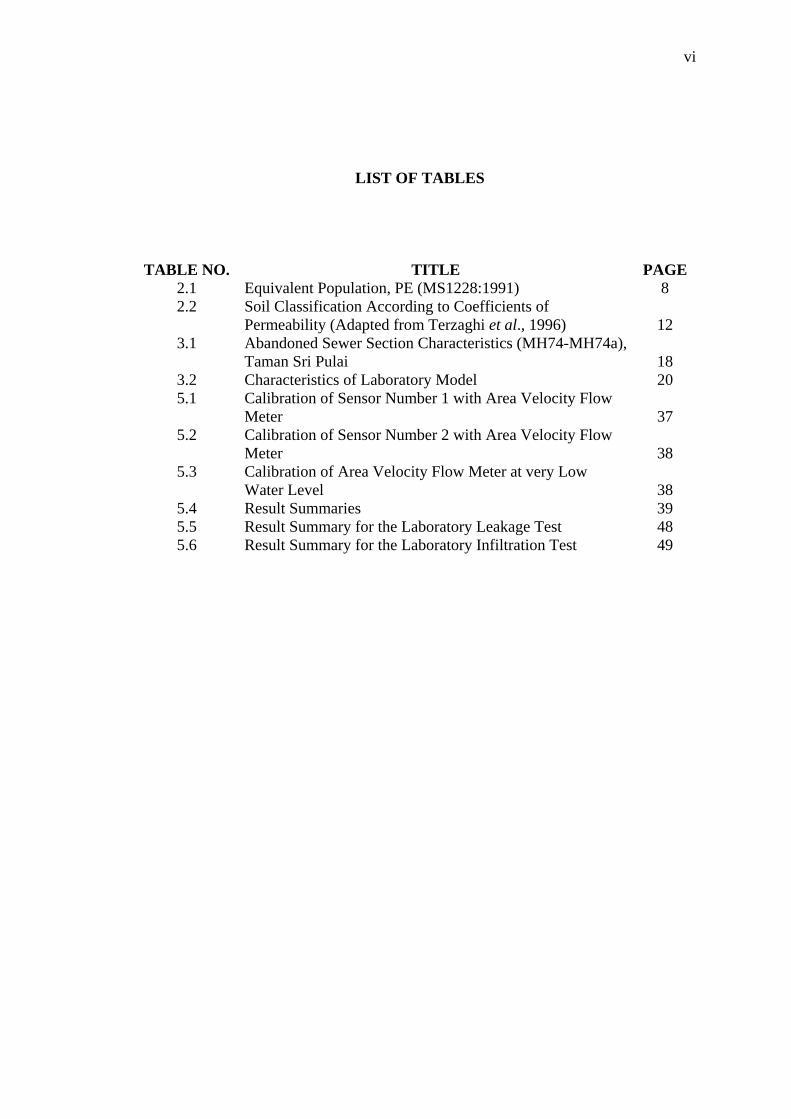
TABLE NO. TITLE PAGE 2.1 Equivalent Population, PE (MS1228:1991) 8 2.2 Soil Classification According to Coefficients of
Permeability (Adapted from Terzaghi et al., 1996)
12 3.1 Abandoned Sewer Section Characteristics (MH74-MH74a),
Taman Sri Pulai
18 3.2 Characteristics of Laboratory Model 20 5.1 Calibration of Sensor Number 1 with Area Velocity Flow
Meter
37 5.2 Calibration of Sensor Number 2 with Area Velocity Flow
Meter
38 5.3 Calibration of Area Velocity Flow Meter at very Low
Water Level
38 5.4 Result Summaries 39 5.5 Result Summary for the Laboratory Leakage Test 48 5.6 Result Summary for the Laboratory Infiltration Test 49
vii
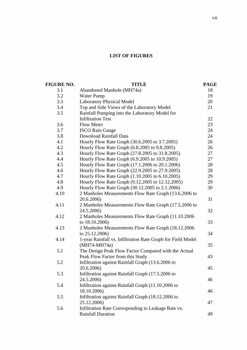
LIST OF FIGURES
FIGURE NO. TITLE PAGE 3.1 Abandoned Manhole (MH74a) 18 3.2 Water Pump 19 3.3 Laboratory Physical Model 20 3.4 Top and Side Views of the Laboratory Model 21 3.5 Rainfall Pumping into the Laboratory Model for
Infiltration Test
22 3.6 Flow Meter 23 3.7 ISCO Rain Gauge 24 3.8 Download Rainfall Data 24 4.1 Hourly Flow Rate Graph (30.6.2005 to 3.7.2005) 26 4.2 Hourly Flow Rate Graph (6.8.2005 to 9.8.2005) 26 4.3 Hourly Flow Rate Graph (27.8.2005 to 31.8.2005) 27 4.4 Hourly Flow Rate Graph (6.9.2005 to 10.9.2005) 27 4.5 Hourly Flow Rate Graph (17.1.2006 to 20.1.2006) 28 4.6 Hourly Flow Rate Graph (22.9.2005 to 27.9.2005) 28 4.7 Hourly Flow Rate Graph (1.10.2005 to 6.10.2005) 29 4.8 Hourly Flow Rate Graph (9.12.2005 to 12.12.2005) 29 4.9 Hourly Flow Rate Graph (30.12.2005 to 2.1.2006) 30 4.10 2 Manholes Measurements Flow Rate Graph (13.6.2006 to
20.6.2006)
31 4.11 2 Manholes Measurements Flow Rate Graph (17.5.2006 to
24.5.2006)
32 4.12 2 Manholes Measurements Flow Rate Graph (11.10.2006
to 18.10.2006)
33 4.13 2 Manholes Measurements Flow Rate Graph (18.12.2006
to 25.12.2006)
34 4.14 1-year Rainfall vs. Infiltration Rate Graph for Field Model
(MH74-MH74a)
35 5.1 The Design Peak Flow Factor Compared with the Actual
Peak Flow Factor from this Study
43 5.2 Infiltration against Rainfall Graph (13.6.2006 to
20.6.2006)
45 5.3 Infiltration against Rainfall Graph (17.5.2006 to
24.5.2006)
46 5.4 Infiltration against Rainfall Graph (11.10.2006 to
18.10.2006)
46 5.5 Infiltration against Rainfall Graph (18.12.2006 to
25.12.2006)
47 5.6 Infiltration Rate Corresponding to Leakage Rate vs.
Rainfall Duration
49
viii
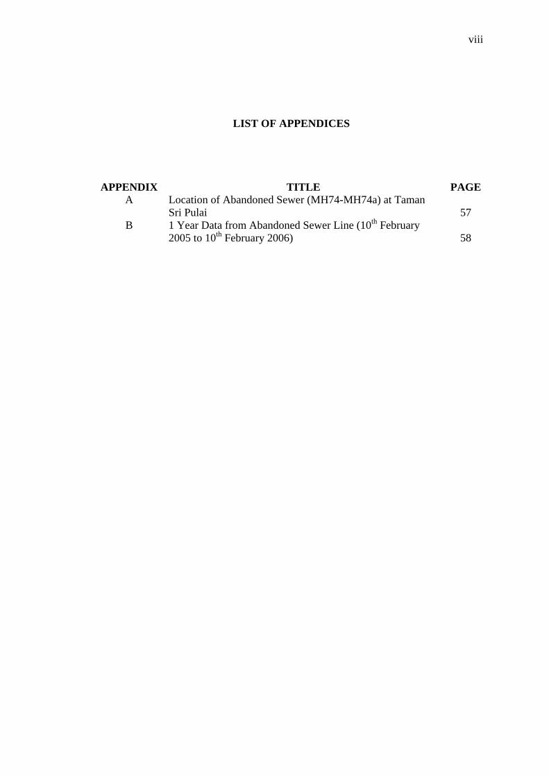
LIST OF APPENDICES
APPENDIX TITLE PAGE A Location of Abandoned Sewer (MH74-MH74a) at Taman
Sri Pulai
57 B 1 Year Data from Abandoned Sewer Line (10th February
2005 to 10th February 2006)
58
CHAPTER 1
INTRODUCTION
1.1 Introduction
A sewerage system is one of the most critical considerations in the sanitary element of any residential, commercial, institutional or industrial construction projects where the final structures will be used by humans for their various activities. This research is currently focused on sewerage system for residential areas and is a joint effort between Indah Water Konsortium (IWK) and Universiti Teknologi Malaysia (UTM).
A sewerage system is a pipe system that carries household and commercial
sewage as well as industrial wastewater toward treatment facilities (Imhoff, 1989). The source can be residential, commercial or industrial area whereas the treatment facilities include activated sludge, oxidation ponds, aerated lagoons, trickling filters and rotating biological contactors.
Sewerage system is very important. It does for people the dirty work of daily
waste disposal, which if not managed properly will result in pollution and contamination of various aspects of our surrounding and ultimately result in adverse effects on human beings, since as stated in Commoner’s Law, “Everything is connected to everything else”. That is why it is so important to make sure that the sewerage systems that exist are functioning well.
The effectiveness of a sewerage system is influenced to a large extent by
infiltration. That is why sewerage system designers cannot look only at the sewage produced from the expected sources like houses, they must also take into serious consideration the effect infiltration has on the sewerage system they are designing, especially in tropical countries where it rains a lot since infiltration becomes critical when it rains. Common sewerage system designs do indeed include an allowance for infiltration but different geographical areas may not experience the same amount of infiltration as estimated by current common practices in sewerage system design. In Malaysia, sewerage systems are designed according to Malaysian Standard Code of Practice MS1228:1991 but in actual fact, MS1228:1991 itself is based on
BS8005:1987 and BS6297:1982 which are in fact conditioned for four season climate and may not be suited to tropical conditions. That is why this research was implemented. 1.2 Problem Statement
Any sewerage system will initially be designed for a specific amount of
sewage only based on the population equivalent (PE) at that time. The design will also include some allowance for infiltration to occur and in Malaysia’s case; the maximum infiltration rate which the sewerage system may be designed for is 50 litres/mm-diameter/km-length/day as stated in MS1228:1991. The design will be adequate if infiltration does not exceed the amount stated but that is usually not the case in tropical climate areas. Kek (1999), Onn (2000), Teh (2001), Cheah (2002), Ho (2002) and Ngoi (2003) have all shown in their study that the amount of infiltration occurring in Malaysia way exceeds the maximum infiltration rate of 50 litres/mm-diameter/km-length/day as stated in MS1228:1991. When the infiltration rate exceeds the amount it is designed for, it will overburden the sewerage system and cause all sorts of negative effects which will be discussed further in the literature review. In view of all the negative effects, a research is desperately needed to study the situation as well as the suitability of the current design criteria for inflow and infiltration in sewerage systems situated in tropical climates. 1.3 Objectives Of Study
i) To study the effect of rainfall on inflow and infiltration patterns in sewerage systems
ii) To determine the optimum design criterion for tropical climate in sewerage systems
iii) To verify the infiltration rate in the sewerage system of Taman Sri Pulai and Taman Universiti
1.4 Scope Of Work
i) Infiltration rate measurement in abandoned sewer line (MH74a-MH74) as a physical field model at Taman Sri Pulai, Skudai, Johor.
ii) Infiltration rate measurement using physical laboratory model at Hidraulic and Hidrology Laboratory, Faculty of Civil Engineering, Universiti Teknologi Malaysia, Skudai, Johor.

iii) Inflow pattern measurement using 1 flowmeter and sensor in manhole (MH11) at Taman Sri Pulai with PE of 1705.
iv) Inflow pattern measurement using 1 flowmeter and sensor in manhole (MH299 & MH1154) at Taman Universiti with PE of 3456 and 9905.
v) Infiltration measurement using 2 flowmeters and sensors in manholes (MH299-MH306 & MH154-MH154a) at Taman Universiti.
vi) Rain intensity measurement using rain gauge at all sites 1.5 Importance Of The Study
Inflow and infiltration is a critical parameter of sewerage system design that
can seriously impair sewerage systems as well as the sewage treatment facilities if not properly studied and implemented.
This research will increase our understanding on the factors causing inflow
and infiltration as well as the effects of inflow and infiltration in sewerage systems. Among the knowledge to be acquired includes the effectiveness of the current standard design used in tropical climate areas. Since the Malaysian Standard on sewerage system design is based on foreign design, it may not be very suitable to tropical conditions even though it can still be used. Besides that, the rate of inflow and infiltration in sewerage systems as well as the ways to overcome them can also be known.
CHAPTER 2
LITERATURE REVIEW
2.1 History
Methods of waste disposal date from ancient times. In his work, Viessman (1985) mentioned that the earliest archeological records of wastewater disposal and central water supply date back to Nippur of Sumeria, about 5000 years back. Wastes from the palaces and the city’s residential areas were transported by an elaborate drainage system. The separate drainage system to collect sewage and rain water individually was first found at the city of Knossos, Greece back around 2000 B.C as written by Mays (2001).
The earliest water treatment knowledge available is in Sanskrit writings which
date back to about 2000 B.C. The writing describes the process of purifying dirty water using 4 steps in succession; boiling in copper vessels, exposure to sunlight, filtering through charcoal and finally cooling in an earthen vessel. The earliest equipment for clarifying water known was found pictured in Egypt around 1500-1300 B.C.
In the year 1627, Sir Francis Bacon wrote on experiments involving water
purification through filtration, boiling, distillation and clarification by coagulation, citing that clarifying water improves health.
In the year 1685, Luc Antonio Porzio published the first known illustrated
description of sand filters, which was focused on conserving the health of soldiers in camps during the Austro-Turkish War. In the 18th and 19th centuries, many experiments on sewerage design were conducted in Russia, Germany, France and England. Viessman (1985) mentioned that Henry Darcy became the first person to apply the laws of hydraulics to filter design and that present day rapid-sand filters were evolved from filters developed in the United States in 1890 which also introduced coagulants for better efficiency.
White (1970) wrote that it was during the Industrial Revolution that the importance of water sanitation systems in towns and urban areas became obvious. Insufficient water supply for waste removal was found in developed urban areas. Water was taken from wherever it can be found; from shallow wells, polluted streams and even leaky water mains which were pressurized for a short period of time every day. Pollution of water supplies results from accumulations of waste matter. A high death rate from dysentery, typhoid, cholera and other types of water-borne diseases was rampant, especially in densely populated areas. Stenis (2004) stated that ‘as urbanization increased, it was no longer possible to employ the natural recycling possible in an agricultural community.’
In view of the poverty and early death resulting from failure of prompt waste
matter removal as well as inadequate supply of clean water, Edwin Chadwick proposed a solution which was immediately sanctioned and became the norm in practice up till this day. His proposal was ‘Each dwelling is supplied internally with clean water, continuously under pressure, and the water used conveys waste matter through a system of pipes at velocity high enough to prevent silting.’ Deposition of solid matter in pipes could be avoided, as shown by John Roe, by using circular cross-section pipes with sufficient gradients provided. 2.2 Types Of Sewerage System
Wastewater is carried from its source to treatment facility pipe systems that
are generally classified according to the type of wastewater flowing through them. If the system carries both domestic and storm-water sewage, it is called a combined system, and these usually serve the older sections of urban areas. As the cities expanded and began to provide treatment of sewage, sanitary sewage was separated from storm sewage by a separate pipe network, called the separate system. This arrangement is more efficient because it excludes the voluminous storm sewage from the treatment plant. It permits flexibility in the operation of the plant and prevents pollution caused by combined sewer overflow, which occurs when the sewer is not big enough to transport both household sewage and storm water. Certain types of sewers, such as inverted siphons and pipes from pumping stations, flow under pressure, and are thus called force mains.
As this research is conducted in Malaysia, it should be made known that the
type of sewerage system adopted in Malaysia is the separate system, with the sanitary sewer network flowing to treatment facilities while the storm sewer network flows to streams, rivers or the sea.

2.3 Transportation Of Wastewater
Households are usually connected to the sewer mains by clay, cast-iron, or polyvinyl chloride (PVC) pipes 8 to 10 centimetres in diametre. Larger-diametre sewer mains can be located along the centerline of a street or alley about 1.8 m or more below the surface. The smaller pipes are usually made of clay, concrete, or asbestos cement, and the large pipes are generally of unlined or lined reinforced-concrete construction. Unlike the water-supply system, wastewater flows through sewer pipes by gravity rather than by pressure. The pipe must be sloped to permit the wastewater to flow at a velocity of at least 0.8 metre per second (MS1228:1991), because at lower velocities the solid material tends to settle in the pipe. Storm-water mains are similar to sanitary sewers except that they have a much larger diametre.
In some places, urban sewer mains discharge into interceptor sewers, which
can then join to form a trunk line that discharges into the wastewater-treatment plant. Interceptors and trunk lines, generally made of brick or reinforced concrete, are sometimes large enough for a truck to pass through them. 2.4 Definition Of Sewer Terms
For the convenience of the reader, many of the terms that the reader will regularly come across in this dissertation are listed here together with their meaning as taken from Hammer & Hammer (2004) and American Society of Civil Engineers (1982).
a) Infiltration – groundwater entering sewers and building connections through defective joints and broken or cracked pipe and manholes.
b) Inflow – water discharged into sewer pipes or service connections from such sources as foundation drains, roof leaders, cellar and yard area drains, cooling water from air conditioners, and other clean-water discharges from commercial and industrial establishments.
c) Wastewater – the spent or used water of a community or industry which contains dissolved and suspended matter.
d) Sanitary Sewer – a sewer that carries liquid and waterborne wastes from residences, commercial buildings, industrial plants, and institutions, together with minor quantities of ground, storm, and surface waters that are not admitted intentionally.
e) Combined Sewer – a sewer intended to receive both wastewater and storm or surface water.
f) Lateral Sewer – a sewer that discharges into a branch or other sewer and has no other common sewer tributary to it.
g) Main Sewer – the principal sewer to which branch sewers and submains are tributary.
h) Trunk Sewer – a sewer that receives many tributary branches and serves a large territory.
i) Intercepting Sewer – a sewer that receives dry-weather flow from a number of transverse sewers or outlets and frequently additional predetermined quantities of storm water from a combined system and conducts such waters to a point for treatment or disposal.
j) Separate Sewer – a sewer intended to receive only wastewater or storm water or surface water.
k) Storm Sewer – a sewer that carries storm water and surface water, street wash and other wash waters, or drainage, but excludes domestic wastewater and industrial wastes.
l) Population Equivalent – the number of persons required to contribute an equivalent quantity of wastewater related to the quantity of flow and strength of Biochemical Oxygen Demand, commonly expressed in terms of BOD5.
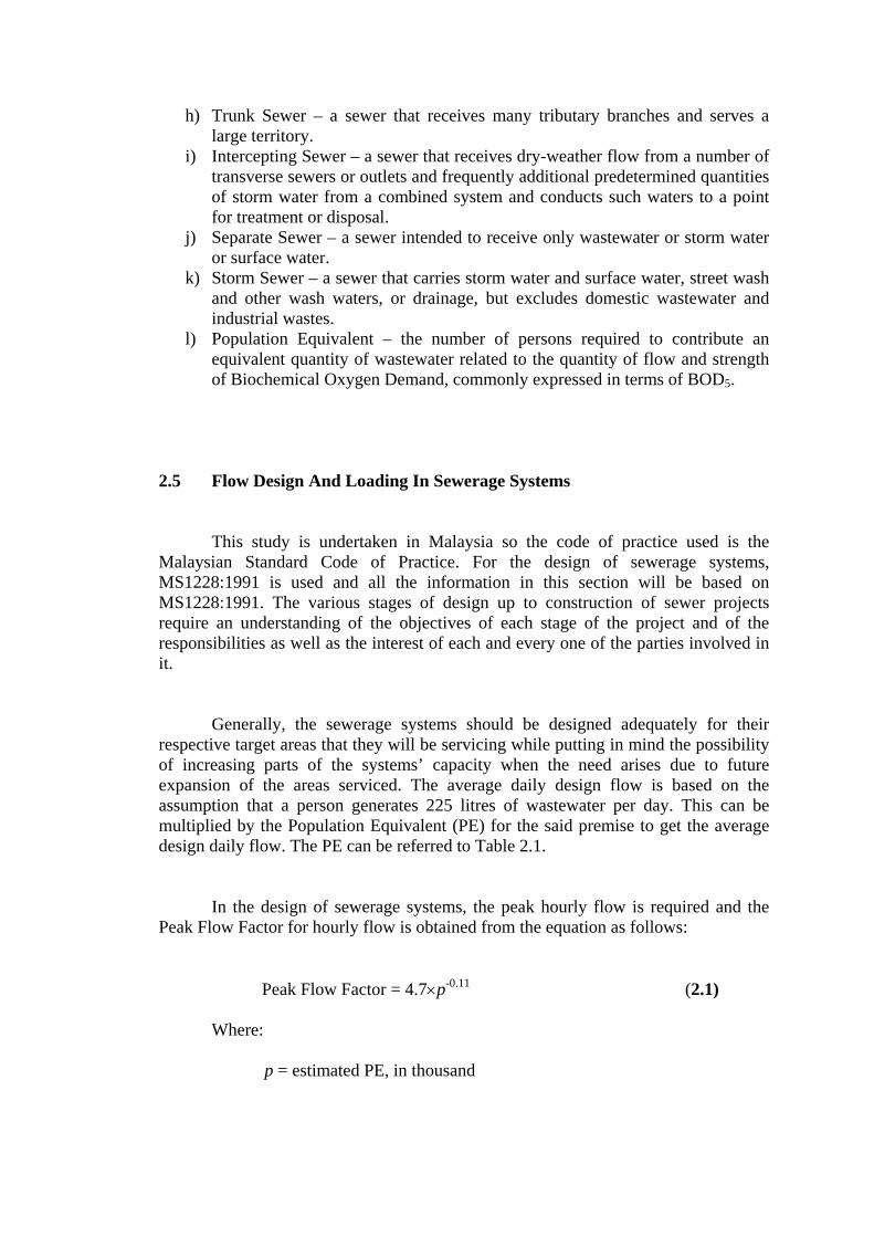
2.5 Flow Design And Loading In Sewerage Systems
This study is undertaken in Malaysia so the code of practice used is the
Malaysian Standard Code of Practice. For the design of sewerage systems, MS1228:1991 is used and all the information in this section will be based on MS1228:1991. The various stages of design up to construction of sewer projects require an understanding of the objectives of each stage of the project and of the responsibilities as well as the interest of each and every one of the parties involved in it.
Generally, the sewerage systems should be designed adequately for their
respective target areas that they will be servicing while putting in mind the possibility of increasing parts of the systems’ capacity when the need arises due to future expansion of the areas serviced. The average daily design flow is based on the assumption that a person generates 225 litres of wastewater per day. This can be multiplied by the Population Equivalent (PE) for the said premise to get the average design daily flow. The PE can be referred to Table 2.1.
In the design of sewerage systems, the peak hourly flow is required and the
Peak Flow Factor for hourly flow is obtained from the equation as follows:
Peak Flow Factor = 4.7×p-0.11 (2.1)
Where:
p = estimated PE, in thousand
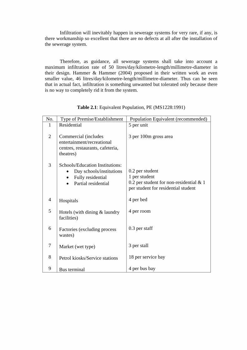
Infiltration will inevitably happen in sewerage systems for very rare, if any, is there workmanship so excellent that there are no defects at all after the installation of the sewerage system.
Therefore, as guidance, all sewerage systems shall take into account a
maximum infiltration rate of 50 litres/day/kilometre-length/millimetre-diameter in their design. Hammer & Hammer (2004) proposed in their written work an even smaller value, 46 litres/day/kilometre-length/millimetre-diameter. Thus can be seen that in actual fact, infiltration is something unwanted but tolerated only because there is no way to completely rid it from the system.
Table 2.1: Equivalent Population, PE (MS1228:1991)
No. Type of Premise/Establishment Population Equivalent (recommended) 1 2 3 4 5 6 7 8 9
Residential Commercial (includes entertainment/recreational centres, restaurants, cafeteria, theatres) Schools/Education Institutions:
• Day schools/institutions • Fully residential • Partial residential
Hospitals Hotels (with dining & laundry facilities) Factories (excluding process wastes) Market (wet type) Petrol kiosks/Service stations Bus terminal
5 per unit 3 per 100m gross area 0.2 per student 1 per student 0.2 per student for non-residential & 1 per student for residential student 4 per bed 4 per room 0.3 per staff 3 per stall 18 per service bay 4 per bus bay
2.6 Factors Contributing To Inflow & Infiltration In Sewerage Systems 2.6.1 Sewer Pipes And Pipe Appurtenances
Much of the infiltration that occurs in sewerage systems is the result of faulty
joints, cracked pipes and manholes as well as joints which are too rigid and not watertight enough. All this happens due to a myriad of reasons, both during and after construction of the sewerage system.
During construction, poor supervision of work by the site supervisor as well as
poor workmanship of the workers may result in faulty joints, cracking of pipes from rough handling, sub-standard fittings and also poor concreting. Besides that, defective material used to construct the sewerage system contributes to infiltration too for they wear out quickly which leads to cracks, fissures and holes where infiltration occurs.
On the other hand, after construction, differential settlement of the soil
beneath the sewer pipes will dislocate the joints of the pipes and create openings for water to seep through. Other than that, unforeseen chemical reactions between the sewer pipes and the inflow contents may damage the insides on the pipes, which may lead to pipe weakening and ultimately cracks and fissures through which infiltration will occur. 2.6.2 Infiltration Through Soil And Soil Properties
Infiltration is the biggest component of rainfall that does not go back to the atmosphere through the hydrologic cycle. It is the process where water from the surface of the earth infiltrates into the soil. Different soil will have different infiltration capacity, stated in mm/hour. It all depends on the soil parameters as well as rain.
To get the rate of infiltration in any particular soil, an infiltrometer is used,
with the most convenient one being the double-ring infiltrometer. The infiltration rate can be obtained using two methods; the Horton Equation and the φ-Index Method.
The Horton Equation is as follows:
f = fc + ( f0 – fc ) e-kt (2.2) Where:
f = Infiltration rate (length/time) f0 = Initial infiltration rate fc = Constant infiltration rate a.k.a. limiting rate k = Recession/Decay constant (time-1) t = Time The infiltration through soil starts at rate f0 and will decrease exponentially
until a constant rate, fc. This is with the assumption that the soil surface is saturated all the time.
The φ-Index Method is a way to obtain the average rain intensity rate where
the volume of surface runoff is taken as the same as effective rainfall. This method is very simplified and is more suited to analyzing storm runoff from large catchment areas but can still be used in this case.
There are many factors which influence infiltration through soil and most of
them are affiliated with the soil property itself. 2.6.2.1 Type Of Soil (Hydraulic Conductivity)
Water can move through soil as saturated flow, unsaturated flow, or vapor flow. Saturated flow takes place when the soil pores are completely filled with water. Unsaturated flow occurs when the larger pores in the soil are filled with air, leaving only the smaller pores to hold and transmit water. Vapor flow occurs as vapor pressure differences develop in relatively dry soils. Vapor migrates from an area of high vapor pressure to an area of low vapor pressure.
Flow through an unsaturated soil is more complicated than flow through
continuously saturated pore spaces. Macropores are filled with air, leaving only finer pores to accommodate water movement. The movement of water in saturated soils is dictated by gravity whereas in unsaturated soils, it is dictated by matric potential. The matric potential gradient is the difference in the matric potential of the moist soil areas, and nearby drier areas into which the water is moving. Moist areas are considered having high matric potential while dry areas have low matric potential.
Hydraulic conductivity is a soil property that describes the ease with which the soil pores permit water, not vapor, movement. It depends on the type of soil, porosity, and the configuration of the soil pores. It is the most important transport property of soil and is a non-linear function of the volumetric water content. Different types of soil will have different hydraulic conductivity, which is stated in the form of i, length/time. The higher the hydraulic conductivity, the lower will be the surface runoff.
Hydraulic conductivity is an important soil property when determining the
potential for infiltration through soil. Soils with high hydraulic conductivities and large pore spaces are likely candidates for heavy infiltration. The hydraulic conductivity in a saturated soil can be measured by injecting a non-reactive tracer like bromide in a monitoring well and measuring the time it takes for the tracer to reach a downgradient monitoring well. 2.6.2.2 Moisture Content
When moisture content is high or the soil is almost saturated, maximum
hydraulic conductivity is achieved very quickly. So when that happens, it will lower surface runoff. When surface runoff is slow, the water tends to seep into the earth and thus add to the infiltration through the soil. 2.6.2.3 Permeability
According to Liu & Evett (2005), permeability refers to the movement of water within soil. The actual movement of water is through voids, which are small, interconnected and irregular conduits. Since water uses voids to move, soils with large voids like sands can usually be considered more permeable than soils such as clays, which have smaller voids. Also, permeability increases in tandem with the increase of void ratio in the soil. Permeability will influence the amount of infiltration through soil because it is related to water movement in soil. The permeability of any type of soil is stated in the form of coefficient of permeability, k, which is usually in metre/second. Table 2.2 shows the degree of permeability for soils according to the value of k.
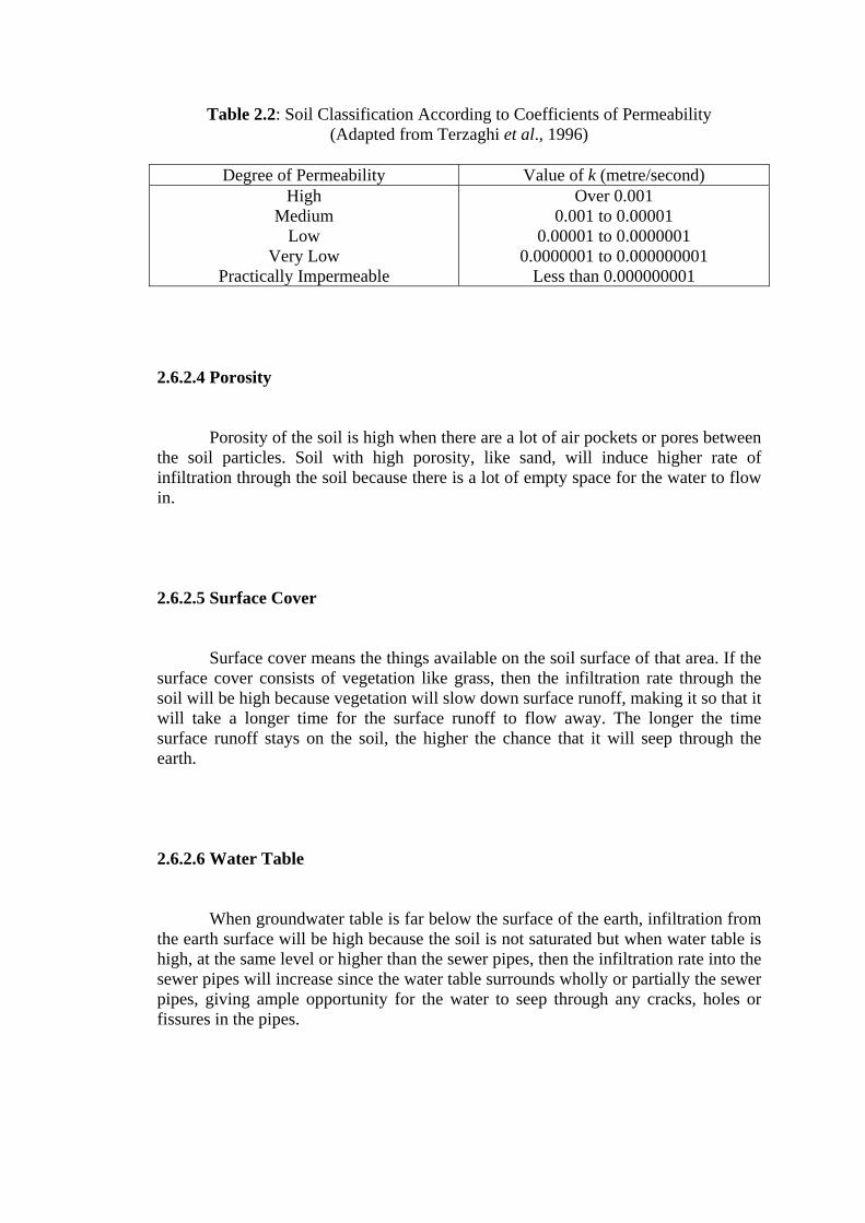
Table 2.2: Soil Classification According to Coefficients of Permeability (Adapted from Terzaghi et al., 1996)
Degree of Permeability Value of k (metre/second)
High Medium
Low Very Low
Practically Impermeable
Over 0.001 0.001 to 0.00001
0.00001 to 0.0000001 0.0000001 to 0.000000001
Less than 0.000000001 2.6.2.4 Porosity
Porosity of the soil is high when there are a lot of air pockets or pores between
the soil particles. Soil with high porosity, like sand, will induce higher rate of infiltration through the soil because there is a lot of empty space for the water to flow in. 2.6.2.5 Surface Cover
Surface cover means the things available on the soil surface of that area. If the
surface cover consists of vegetation like grass, then the infiltration rate through the soil will be high because vegetation will slow down surface runoff, making it so that it will take a longer time for the surface runoff to flow away. The longer the time surface runoff stays on the soil, the higher the chance that it will seep through the earth. 2.6.2.6 Water Table
When groundwater table is far below the surface of the earth, infiltration from
the earth surface will be high because the soil is not saturated but when water table is high, at the same level or higher than the sewer pipes, then the infiltration rate into the sewer pipes will increase since the water table surrounds wholly or partially the sewer pipes, giving ample opportunity for the water to seep through any cracks, holes or fissures in the pipes.
2.6.2.7 Rain The effect of rain on inflow and infiltration depends on the intensity, the
duration and the volume of the rain. As the intensity increase, infiltration through the soil decreases because most of the rain will be washed away as surface runoff. A large part will not be able to percolate through the soil and vice versa. For duration, it is the opposite. A longer duration will give higher infiltration rate because the surface runoff is less and there is more time for it to seep into the soil. The same goes for volume. The higher the volume, of course the more infiltration can happen. In tropical countries, the weather is divided into wet season and dry season. During the wet season, there is a lot of rain and thunderstorms so infiltration will increase in those periods of time.
2.6.3 Population Increase The population of this world is ever-increasing and even the sewerage systems
of this world are not spared the effect of this. Even though the sewerage system is designed for the population equivalent at the end of its service period, when the number of users using the sewerage system exceeds that value, it will overburden the sewerage system because the system does not have the capacity to support the additional sewage. If there is prolonged overburden of the sewerage system, it will likely cause cracks and other adverse effects, which will lead to infiltration. In severe cases, failure of the whole sewerage system will result. 2.6.4 Passage Of Time
As time goes by, a sewerage system will deteriorate due to wear and tear as it
performs the daily task of wastewater disposal. So it can be safely said that all the sewerage systems will deteriorate with time and with the deterioration comes the unwanted inflow and infiltration in increasing proportions.

2.7 Effects Of Inflow And Infiltration In many existing sanitary sewers infiltration is a major cause of hydraulic
overloading of both the collection system and treatment plant. To handle this excess flow it may become necessary to construct relief sewers and expand existing treatment facilities. So, clean water infiltration into sanitary sewers should be avoided whenever possible. The following is a number of adverse effects that excessive inflow and infiltration will have on the sewerage systems.
1) Surcharging of sewer lines with back-up of sanitary wastewaters into
house basements 2) Reducing the capacity of the sewer for conveying the waste flows for
which it was designed 3) Higher pumping costs 4) Treatment plant hydraulic overloads, thus the bypass and overflow of
untreated sewage into receiving waters 5) Flooding of street and road areas 6) Cave-ins and structural failures in sewers and pavements resulting from
soil washing into the sewer 7) Higher maintenance costs resulting from soil deposits in sewers, additional
root penetration into leaky joints, etc 8) Entrance of spores of bacterial and other organisms through the infiltration
water
CHAPTER 3
METHODOLOGY
3.1 Introduction
Methodology is the statement of how the proposed research will be done. In this research, it will involve conducting different types of measurement to get different values that will ultimately be used in the endeavour to reach the objectives of this research. In this methodology chapter, the techniques to obtain the different data like rainfall intensity and flow from site will be stated and shown. 3.2 Preliminary Works
The term preliminary in this situation means the initial works that the author
had to do before moving to the real data collection at site. This includes information gathering on the topic of inflow and infiltration, past dissertation reviews, self-study on similar and related topics in order to learn more. Site visits are also conducted to assess the situation and the best way to go about collecting data. 3.2.1 Information Gathering
A wide array of journals, books and articles has to be read in order to obtain information on the topic of inflow and infiltration. Sources mostly come from abroad since this topic is relatively new in Malaysia and very few local studies have been conducted.
3.2.3 Site Visits Site visit have been conducted to Taman Sri Pulai (MH74-MH74a & MH11-
MH13a) and Taman Universiti (MH299-MH306 & MH154-MH154a) with the help of location maps obtained from the relevant authorities before any work can proceed at those sites. A special trip to Shah Alam has also been conducted on the 21st and 22nd of January 2006, specifically to visit our future site, Taman with a PE of 18000. Site visits are necessary because we can know the actual location of the site of work and the ground conditions first hand. 3.3 Site Work
After the preliminary work is done and all is prepared, the site work can begin. In this study there are 3 sites namely Taman Sri Pulai, Taman Universiti and Shah Alam. The work in Taman Sri Pulai encompasses flow characteristics study and pure infiltration study while the work in Taman Universiti includes flow characteristics study and inflow & infiltration study. In Shah Alam, the work will be inflow and infiltration measurement. For all these sites, the PE is different and the rainfall intensity is constantly measured. 3.3.1 Population Equivalent (PE) Determination
The PE for the section of the sewerage pipe where the study is implemented can usually be obtained from either the developer or the sewerage service provider. In order to check the accuracy of the PE obtained as well as any increase or decrease from the initial PE value, a recount of PE is scheduled for each of the different site. 3.3.2 Flow Characteristics Measurement
The measurement for flow characteristics of a section of sewerage pipe systems is done using 1 flowmeter complete with sensor. In this study, the flowmeter used is the 4250 Area-Velocity Flow Meter, and it will automatically record the flow, velocity and water height at preset intervals, which in this case is 5 minutes. Once a measurement is complete regardless of the duration, the data from the flowmeter will be downloaded into a computer which has the Flowlink4 software. This software enables the plotting of graphs for the 3 parameters downloaded as well as transfer of data to other software’s for the user’s convenience.
From the flow measurements, we can get Q maximum hourly, Q minimum hourly and Q average with Q being the flow. From Q average, we can get the per capita flow by using the following equation:
Flow per capita
= Average daily flow (m3/day) ÷ (3.1) Total population equivalent (PE)
= m3/day/person Examination of wastewater flow characteristics can also be done through a
data that are obtained from the field experiment. The information that related to design sewerage systems are as following:
a. Peak flow factor = 4.7 × p-0.11 (3.2) b. Average domestic flow = Flow per capita × PE (3.3)
= m3/day c. Peak domestic flow
= Peak flow factor × Average domestic flow (3.4) = 4.7 × p-0.11 × Flow per capita × PE = m3/day
The ‘p’ value is an estimated PE in thousands (in section 3.6, MS 1228:1991). The average flow per capita used by Malaysian Standard is 0.225 m3/day/person (in section 3.2, MS 1228:1991).
Following is the formulae used in obtaining infiltration rate for measuring wastewater flow at 2 manholes:
Infiltration rate (for 2 manholes flow measurement)
= [Downstream flow (Q out) – Upstream flow (Q in)] ÷ (3.5) [Pipe length × Pipe diameter]
= l/day /km/mm-diameter 3.3.3 Infiltration Measurement
As mentioned in Section 2.4, infiltration is additional unwanted extraneous
water in sewerage systems. In this study, the infiltration measurement is divided into 2 parts, pure infiltration measurement and inflow plus infiltration measurement.
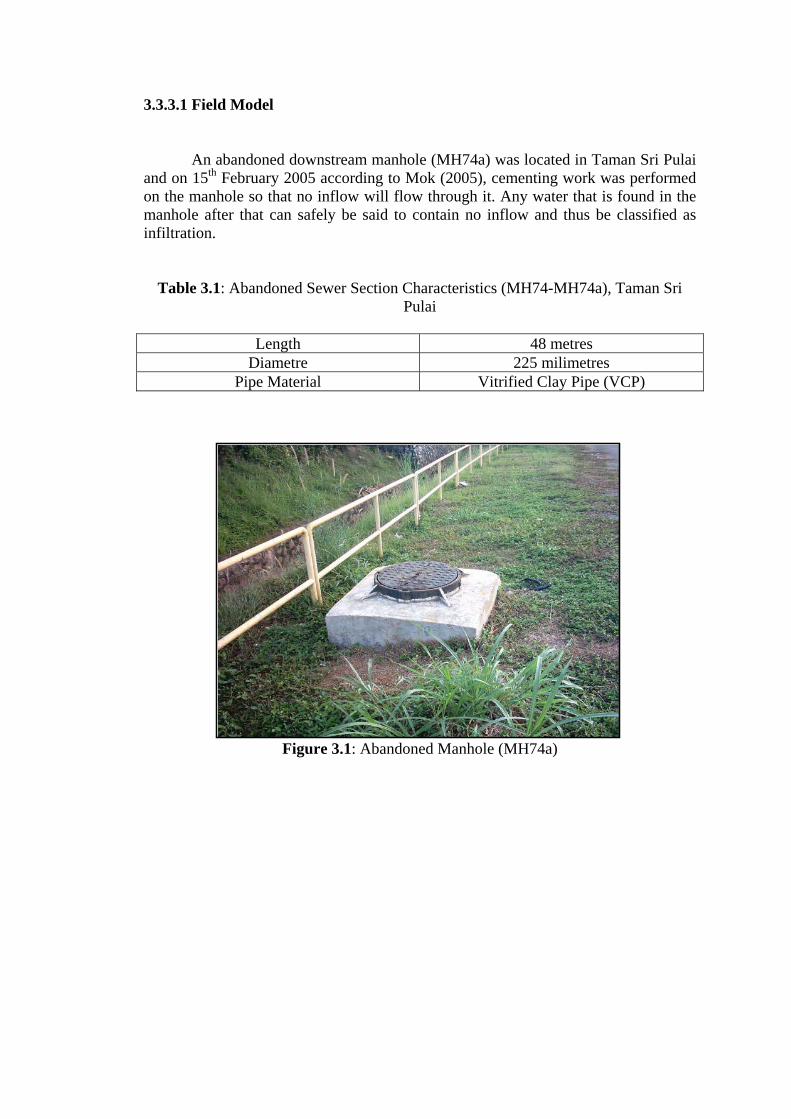
3.3.3.1 Field Model
An abandoned downstream manhole (MH74a) was located in Taman Sri Pulai and on 15th February 2005 according to Mok (2005), cementing work was performed on the manhole so that no inflow will flow through it. Any water that is found in the manhole after that can safely be said to contain no inflow and thus be classified as infiltration.
Table 3.1: Abandoned Sewer Section Characteristics (MH74-MH74a), Taman Sri Pulai
Length 48 metres
Diametre 225 milimetres Pipe Material Vitrified Clay Pipe (VCP)
Figure 3.1: Abandoned Manhole (MH74a)
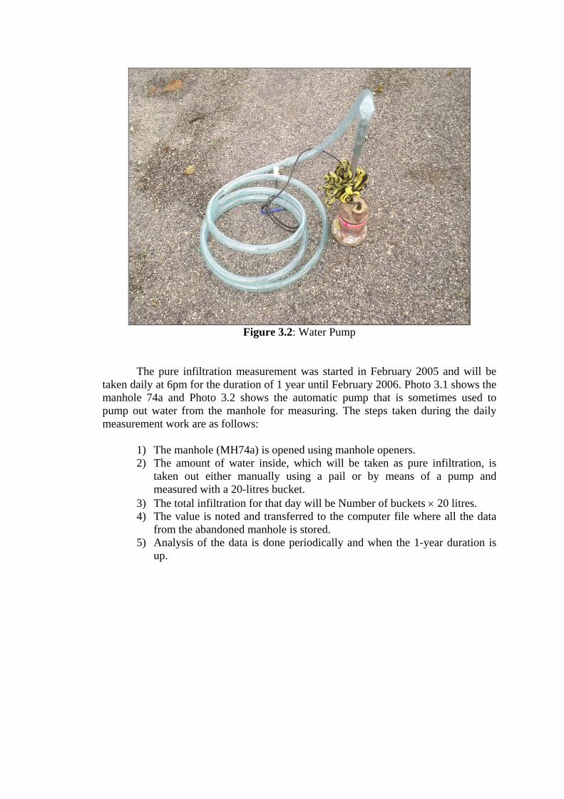
Figure 3.2: Water Pump
The pure infiltration measurement was started in February 2005 and will be taken daily at 6pm for the duration of 1 year until February 2006. Photo 3.1 shows the manhole 74a and Photo 3.2 shows the automatic pump that is sometimes used to pump out water from the manhole for measuring. The steps taken during the daily measurement work are as follows:
1) The manhole (MH74a) is opened using manhole openers. 2) The amount of water inside, which will be taken as pure infiltration, is
taken out either manually using a pail or by means of a pump and measured with a 20-litres bucket.
3) The total infiltration for that day will be Number of buckets × 20 litres. 4) The value is noted and transferred to the computer file where all the data
from the abandoned manhole is stored. 5) Analysis of the data is done periodically and when the 1-year duration is
up.
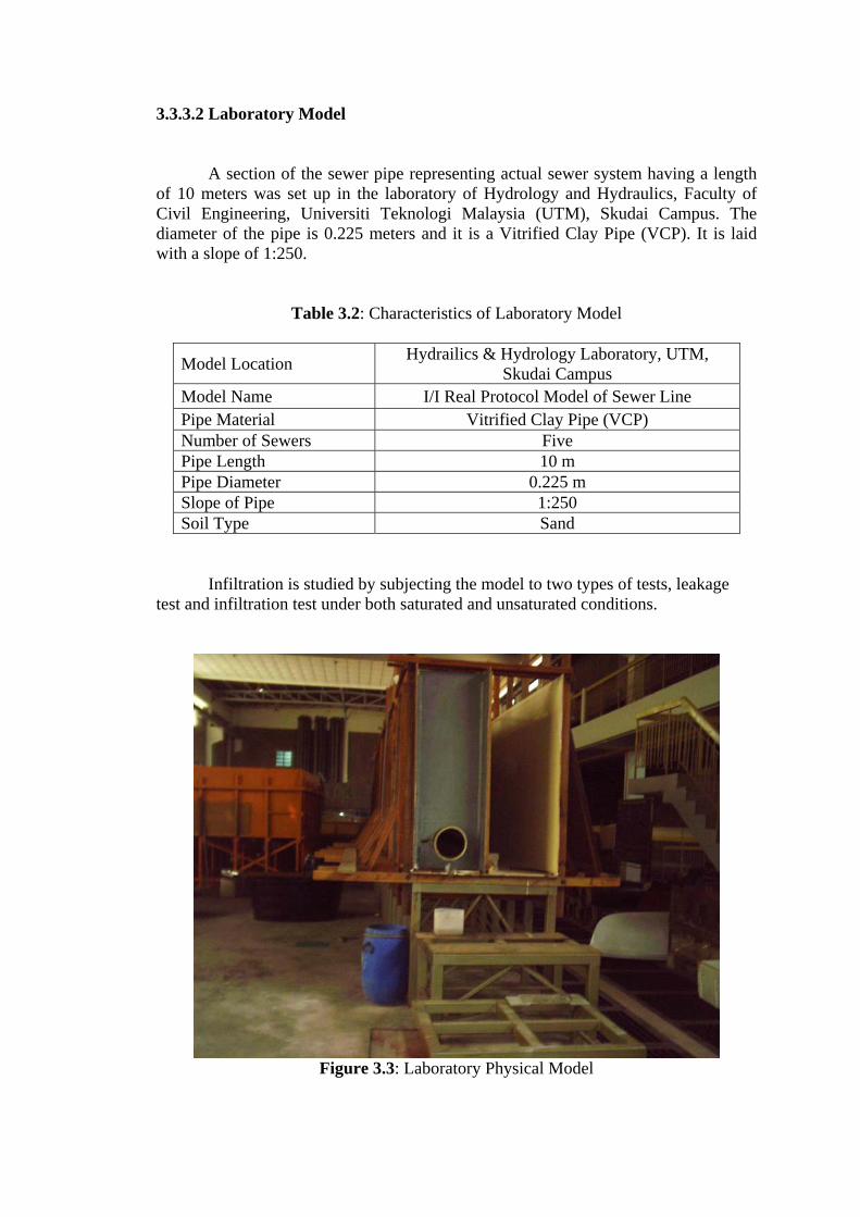
3.3.3.2 Laboratory Model
A section of the sewer pipe representing actual sewer system having a length of 10 meters was set up in the laboratory of Hydrology and Hydraulics, Faculty of Civil Engineering, Universiti Teknologi Malaysia (UTM), Skudai Campus. The diameter of the pipe is 0.225 meters and it is a Vitrified Clay Pipe (VCP). It is laid with a slope of 1:250.
Table 3.2: Characteristics of Laboratory Model
Model Location Hydrailics & Hydrology Laboratory, UTM, Skudai Campus
Model Name I/I Real Protocol Model of Sewer Line Pipe Material Vitrified Clay Pipe (VCP) Number of Sewers Five Pipe Length 10 m Pipe Diameter 0.225 m Slope of Pipe 1:250 Soil Type Sand
Infiltration is studied by subjecting the model to two types of tests, leakage test and infiltration test under both saturated and unsaturated conditions.
Figure 3.3: Laboratory Physical Model
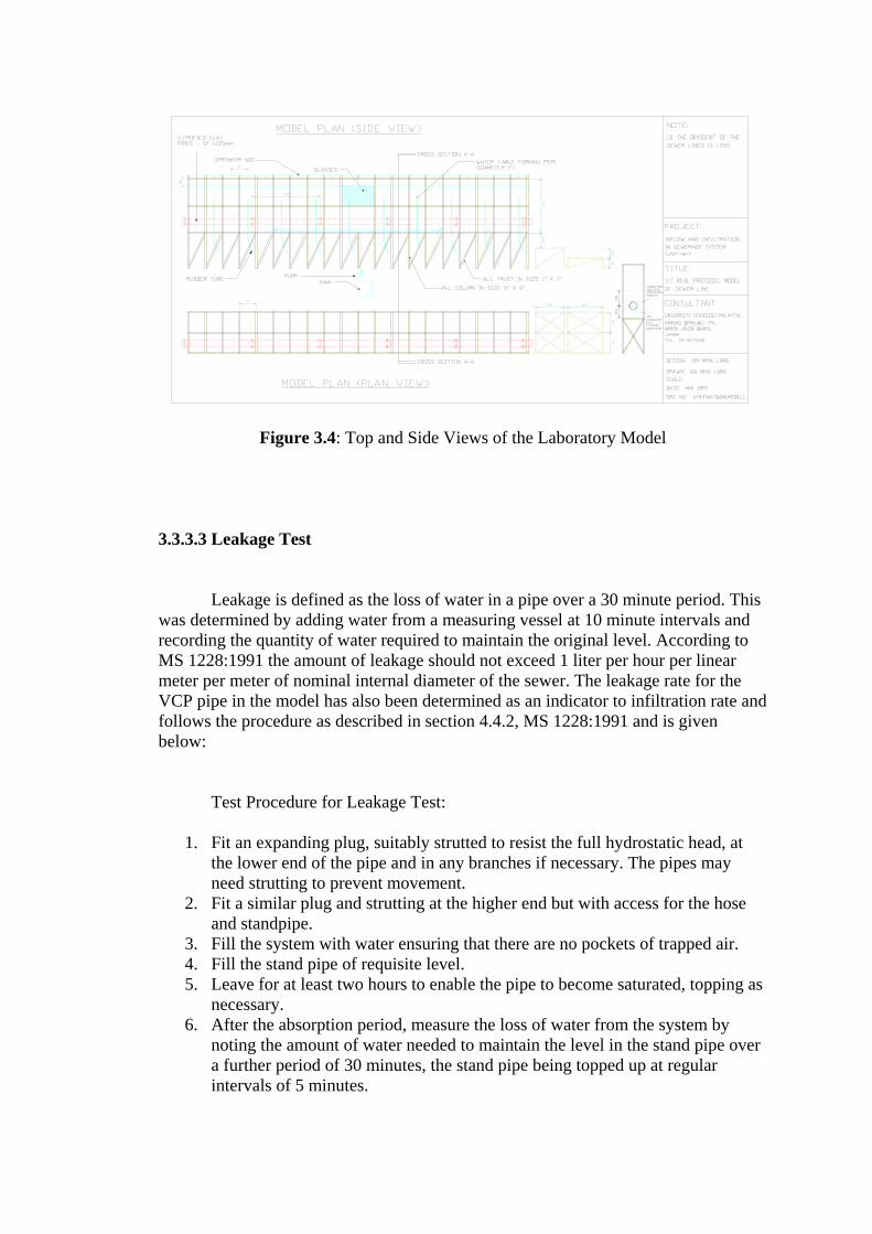
Figure 3.4: Top and Side Views of the Laboratory Model
3.3.3.3 Leakage Test
Leakage is defined as the loss of water in a pipe over a 30 minute period. This was determined by adding water from a measuring vessel at 10 minute intervals and recording the quantity of water required to maintain the original level. According to MS 1228:1991 the amount of leakage should not exceed 1 liter per hour per linear meter per meter of nominal internal diameter of the sewer. The leakage rate for the VCP pipe in the model has also been determined as an indicator to infiltration rate and follows the procedure as described in section 4.4.2, MS 1228:1991 and is given below:
Test Procedure for Leakage Test:
1. Fit an expanding plug, suitably strutted to resist the full hydrostatic head, at the lower end of the pipe and in any branches if necessary. The pipes may need strutting to prevent movement.
2. Fit a similar plug and strutting at the higher end but with access for the hose and standpipe.
3. Fill the system with water ensuring that there are no pockets of trapped air. 4. Fill the stand pipe of requisite level. 5. Leave for at least two hours to enable the pipe to become saturated, topping as
necessary. 6. After the absorption period, measure the loss of water from the system by
noting the amount of water needed to maintain the level in the stand pipe over a further period of 30 minutes, the stand pipe being topped up at regular intervals of 5 minutes.
3.3.3.4 Infiltration Test
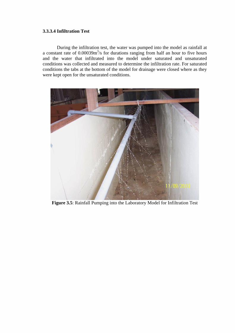
During the infiltration test, the water was pumped into the model as rainfall at a constant rate of 0.00039m3/s for durations ranging from half an hour to five hours and the water that infiltrated into the model under saturated and unsaturated conditions was collected and measured to determine the infiltration rate. For saturated conditions the tabs at the bottom of the model for drainage were closed where as they were kept open for the unsaturated conditions.
Figure 3.5: Rainfall Pumping into the Laboratory Model for Infiltration Test
3.3.3.5 Inflow & Infiltration
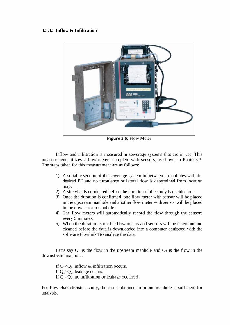
Figure 3.6: Flow Meter
Inflow and infiltration is measured in sewerage systems that are in use. This measurement utilizes 2 flow meters complete with sensors, as shown in Photo 3.3. The steps taken for this measurement are as follows:
1) A suitable section of the sewerage system in between 2 manholes with the
desired PE and no turbulence or lateral flow is determined from location map.
2) A site visit is conducted before the duration of the study is decided on. 3) Once the duration is confirmed, one flow meter with sensor will be placed
in the upstream manhole and another flow meter with sensor will be placed in the downstream manhole.
4) The flow meters will automatically record the flow through the sensors every 5 minutes.
5) When the duration is up, the flow meters and sensors will be taken out and cleaned before the data is downloaded into a computer equipped with the software Flowlink4 to analyze the data.
Let’s say Q1 is the flow in the upstream manhole and Q2 is the flow in the
downstream manhole. If Q1<Q2, inflow & infiltration occurs. If Q1>Q2, leakage occurs. If Q1=Q2, no infiltration or leakage occurred
For flow characteristics study, the result obtained from one manhole is sufficient for analysis.
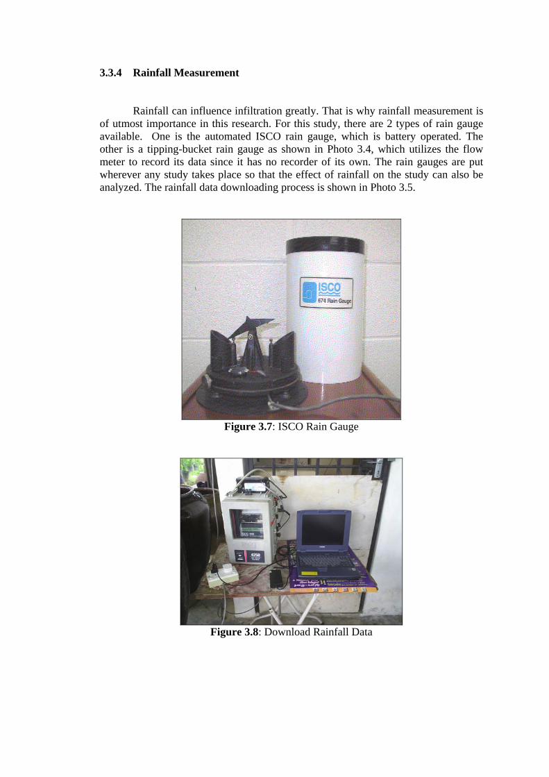
3.3.4 Rainfall Measurement Rainfall can influence infiltration greatly. That is why rainfall measurement is
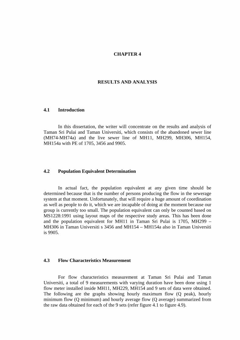
of utmost importance in this research. For this study, there are 2 types of rain gauge available. One is the automated ISCO rain gauge, which is battery operated. The other is a tipping-bucket rain gauge as shown in Photo 3.4, which utilizes the flow meter to record its data since it has no recorder of its own. The rain gauges are put wherever any study takes place so that the effect of rainfall on the study can also be analyzed. The rainfall data downloading process is shown in Photo 3.5.
Figure 3.7: ISCO Rain Gauge
Figure 3.8: Download Rainfall Data
CHAPTER 4
RESULTS AND ANALYSIS
4.1 Introduction
In this dissertation, the writer will concentrate on the results and analysis of Taman Sri Pulai and Taman Universiti, which consists of the abandoned sewer line (MH74-MH74a) and the live sewer line of MH11, MH299, MH306, MH154, MH154a with PE of 1705, 3456 and 9905. 4.2 Population Equivalent Determination
In actual fact, the population equivalent at any given time should be determined because that is the number of persons producing the flow in the sewerage system at that moment. Unfortunately, that will require a huge amount of coordination as well as people to do it, which we are incapable of doing at the moment because our group is currently too small. The population equivalent can only be counted based on MS1228:1991 using layout maps of the respective study areas. This has been done and the population equivalent for MH11 in Taman Sri Pulai is 1705, MH299 – MH306 in Taman Universiti s 3456 and MH154 – MH154a also in Taman Universiti is 9905. 4.3 Flow Characteristics Measurement
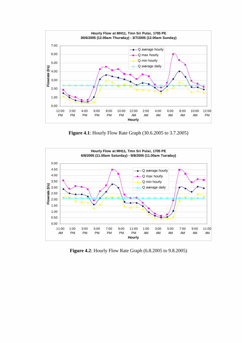
For flow characteristics measurement at Taman Sri Pulai and Taman Universiti, a total of 9 measurements with varying duration have been done using 1 flow meter installed inside MH11, MH229, MH154 and 9 sets of data were obtained. The following are the graphs showing hourly maximum flow (Q peak), hourly minimum flow (Q minimum) and hourly average flow (Q average) summarized from the raw data obtained for each of the 9 sets (refer figure 4.1 to figure 4.9).
Hourly Flow at MH11, Tmn Sri Pulai, 1705 PE 30/6/2005 (12.00am Thursday) - 3/7/2005 (12.00am Sunday)
0.00
1.00
2.00
3.00
4.00
5.00
6.00
7.00
12:00PM
2:00PM
4:00PM
6:00PM
8:00PM
10:00PM
12:00AM
2:00AM
4:00AM
6:00AM
8:00AM
10:00AM
12:00PM
Hourly
Flow
rate
(l/s
)Q average hourlyQ max hourlyQ min hourlyQ average daily
Figure 4.1: Hourly Flow Rate Graph (30.6.2005 to 3.7.2005)
Hourly Flow at MH11, Tmn Sri Pulai, 1705 PE 6/8/2005 (11.00am Saturday) - 9/8/2005 (11.00am Tuesday)
0.00
0.50
1.00
1.50
2.00
2.50
3.00
3.50
4.00
4.50
5.00
11:00AM
1:00PM
3:00PM
5:00PM
7:00PM
9:00PM
11:00PM
1:00AM
3:00AM
5:00AM
7:00AM
9:00AM
11:00AM
Hourly
Flow
rate
(l/s
)
Q average hourlyQ max hourlyQ min hourlyQ average daily
Figure 4.2: Hourly Flow Rate Graph (6.8.2005 to 9.8.2005)
Hourly Flow at MH11, Tmn Sri Pulai, 1705 PE 27/8/2005 (12.00am Saturday) - 31/8/2005 (12.00am Wednesday)
0.00
1.00
2.00
3.00
4.00
5.00
6.00
7.00
12:00AM
2:00AM
4:00AM
6:00AM
8:00AM
10:00AM
12:00PM
2:00PM
4:00PM
6:00PM
8:00PM
10:00PM
12:00AM
Hourly
Flow
rate
(l/s
)Q average hourlyQ max hourlyQ min hourlyQ average daily
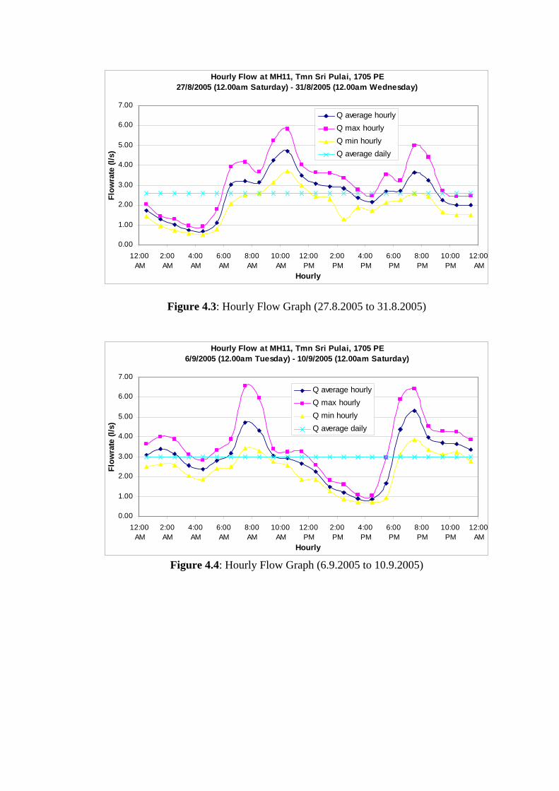
Figure 4.3: Hourly Flow Graph (27.8.2005 to 31.8.2005)
Hourly Flow at MH11, Tmn Sri Pulai, 1705 PE 6/9/2005 (12.00am Tuesday) - 10/9/2005 (12.00am Saturday)
0.00
1.00
2.00
3.00
4.00
5.00
6.00
7.00
12:00AM
2:00AM
4:00AM
6:00AM
8:00AM
10:00AM
12:00PM
2:00PM
4:00PM
6:00PM
8:00PM
10:00PM
12:00AM
Hourly
Flow
rate
(l/s
)
Q average hourlyQ max hourlyQ min hourlyQ average daily
Figure 4.4: Hourly Flow Graph (6.9.2005 to 10.9.2005)
Hourly Flow at MH11, Tmn Sri Pulai, 1705 PE17/1/2006 (3.00pm Tuesday) - 20/1/2006 (3.00pm Friday)
0.00
1.00
2.00
3.00
4.00
5.00
6.00
7.00
8.00
9.00
3:00PM
5:00PM
7:00PM
9:00PM
11:00PM
1:00AM
3:00AM
5:00AM
7:00AM
9:00AM
11:00AM
1:00PM
3:00PM
Hourly
Flow
rate
(l/s
)Q average hourlyQ max hourlyQ min hourlyQ average daily
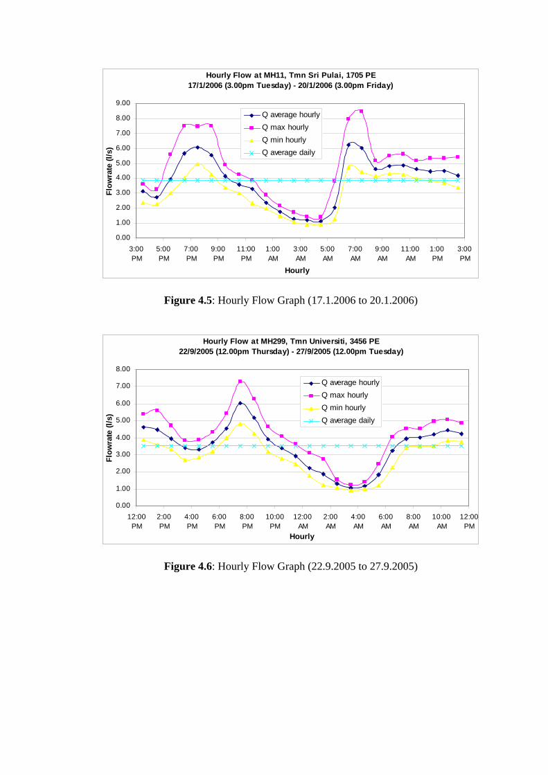
Figure 4.5: Hourly Flow Graph (17.1.2006 to 20.1.2006)
Hourly Flow at MH299, Tmn Universiti, 3456 PE 22/9/2005 (12.00pm Thursday) - 27/9/2005 (12.00pm Tuesday)
0.00
1.00
2.00
3.00
4.00
5.00
6.00
7.00
8.00
12:00PM
2:00PM
4:00PM
6:00PM
8:00PM
10:00PM
12:00AM
2:00AM
4:00AM
6:00AM
8:00AM
10:00AM
12:00PM
Hourly
Flow
rate
(l/s
)
Q average hourlyQ max hourlyQ min hourlyQ average daily
Figure 4.6: Hourly Flow Graph (22.9.2005 to 27.9.2005)
Hourly Flow at MH299, Tmn Universiti, 3456 PE 1/10/2005 (12.00am Saturday) - 6/10/2005 (12.00am Thursday)
0.00
1.00
2.00
3.00
4.00
5.00
6.00
7.00
8.00
9.00
12:00AM
2:00AM
4:00AM
6:00AM
8:00AM
10:00AM
12:00PM
2:00PM
4:00PM
6:00PM
8:00PM
10:00PM
12:00AM
Hourly
Flow
rate
(l/s
)
Q average hourlyQ max hourlyQ min hourlyQ average daily
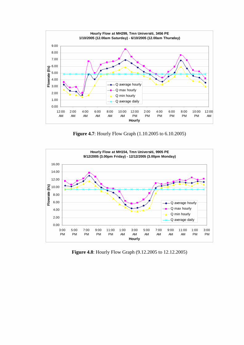
Figure 4.7: Hourly Flow Graph (1.10.2005 to 6.10.2005)
Hourly Flow at MH154, Tmn Universiti, 9905 PE9/12/2005 (3.00pm Friday) - 12/12/2005 (3.00pm Monday)
0.00
2.00
4.00
6.00
8.00
10.00
12.00
14.00
16.00
3:00PM
5:00PM
7:00PM
9:00PM
11:00PM
1:00AM
3:00AM
5:00AM
7:00AM
9:00AM
11:00AM
1:00PM
3:00PM
Hourly
Flow
rate
(l/s
)
Q average hourlyQ max hourlyQ min hourlyQ average daily
Figure 4.8: Hourly Flow Graph (9.12.2005 to 12.12.2005)
Hourly Flow at MH154, Tmn Universiti, 9905 PE30/12/2005 (12.00pm Friday) - 2/1/2006 (12.00pm Monday)
0.00
2.00
4.00
6.00
8.00
10.00
12.00
14.00
16.00
18.00
12:00PM
2:00PM
4:00PM
6:00PM
8:00PM
10:00PM
12:00AM
2:00AM
4:00AM
6:00AM
8:00AM
10:00AM
12:00PM
Hourly
Flow
rate
(l/s
)Q average hourlyQ max hourlyQ min hourlyQ average daily
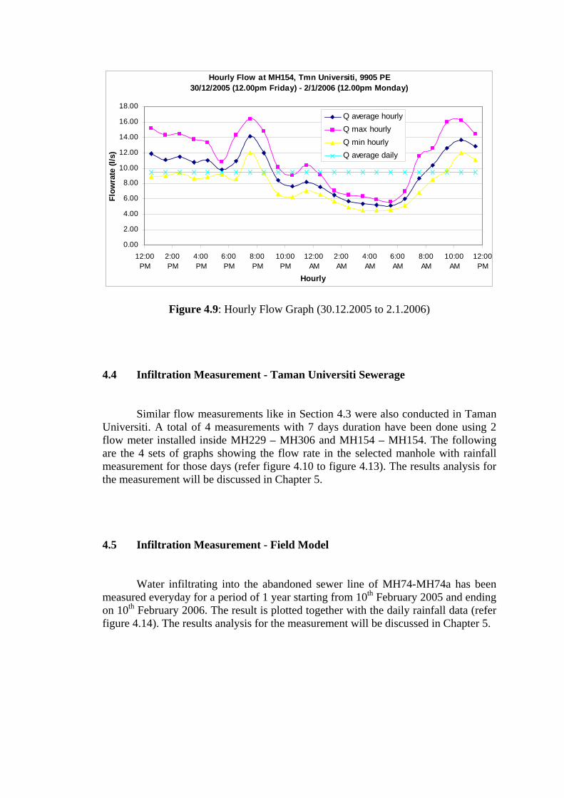
Figure 4.9: Hourly Flow Graph (30.12.2005 to 2.1.2006) 4.4 Infiltration Measurement - Taman Universiti Sewerage
Similar flow measurements like in Section 4.3 were also conducted in Taman
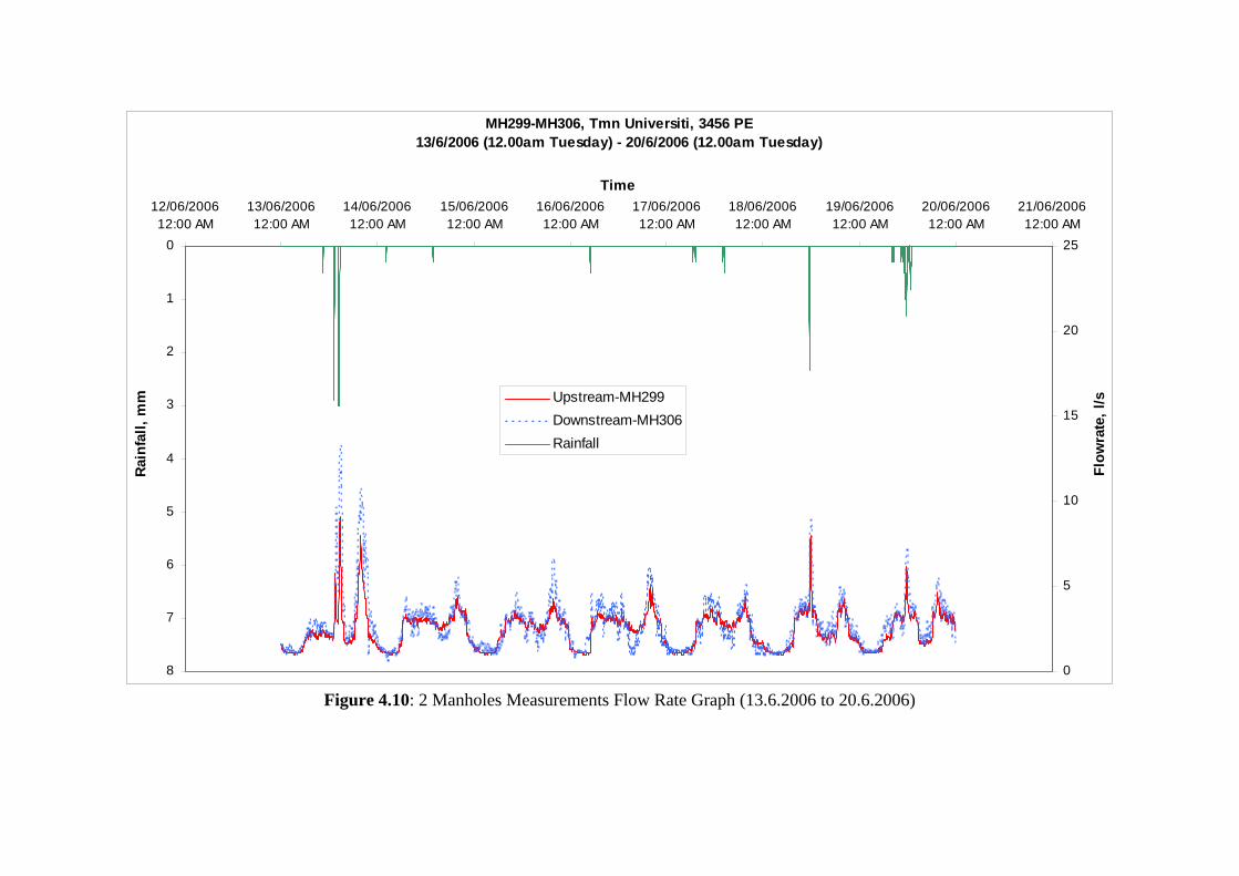
Universiti. A total of 4 measurements with 7 days duration have been done using 2 flow meter installed inside MH229 – MH306 and MH154 – MH154. The following are the 4 sets of graphs showing the flow rate in the selected manhole with rainfall measurement for those days (refer figure 4.10 to figure 4.13). The results analysis for the measurement will be discussed in Chapter 5. 4.5 Infiltration Measurement - Field Model
Water infiltrating into the abandoned sewer line of MH74-MH74a has been measured everyday for a period of 1 year starting from 10th February 2005 and ending on 10th February 2006. The result is plotted together with the daily rainfall data (refer figure 4.14). The results analysis for the measurement will be discussed in Chapter 5.
MH299-MH306, Tmn Universiti, 3456 PE13/6/2006 (12.00am Tuesday) - 20/6/2006 (12.00am Tuesday)
0
1
2
3
4
5
6
7
8
12/06/200612:00 AM
13/06/200612:00 AM
14/06/200612:00 AM
15/06/200612:00 AM
16/06/200612:00 AM
17/06/200612:00 AM
18/06/200612:00 AM
19/06/200612:00 AM
20/06/200612:00 AM
21/06/200612:00 AM
Time
Rain
fall,
mm
0
5
10
15
20
25
Flow
rate
, l/sUpstream-MH299
Downstream-MH306Rainfall
Figure 4.10: 2 Manholes Measurements Flow Rate Graph (13.6.2006 to 20.6.2006)
MH154-MH154a, Tmn Universiti, 9905 PE17/5/2006 (12.00pm Wednesday) - 24/5/2006 (12.00pm Wednesday)
0
5
10
15
20
25
30
17/05/200612:00 AM
18/05/200612:00 AM
19/05/200612:00 AM
20/05/200612:00 AM
21/05/200612:00 AM
22/05/200612:00 AM
23/05/200612:00 AM
24/05/200612:00 AM
25/05/200612:00 AM
Time
Rain
fall,
mm
0
20
40
60
80
100
120
140
Flow
rate
, l/s
Upstream-MH154 Downstream-MH154aRainfall
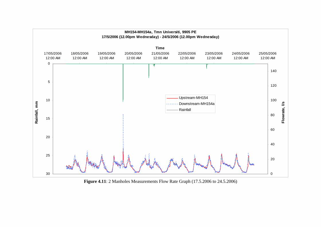
Figure 4.11: 2 Manholes Measurements Flow Rate Graph (17.5.2006 to 24.5.2006)
MH154-MH154a, Tmn Universiti, 9905 PE11/10/2006 (12.00am Wednesday) - 18/10/2006 (12.00am Wednesday)
0
20
40
60
80
100
120
140
10/10/200612:00 AM
11/10/200612:00 AM
12/10/200612:00 AM
13/10/200612:00 AM
14/10/200612:00 AM
15/10/200612:00 AM
16/10/200612:00 AM
17/10/200612:00 AM
18/10/200612:00 AM
19/10/200612:00 AM
Time
Rain
fall,
mm
0
20
40
60
80
100
120
140
160
180
200
Flow
rate
, l/s
Upstream-MH154Downstream-MH154aRainfall
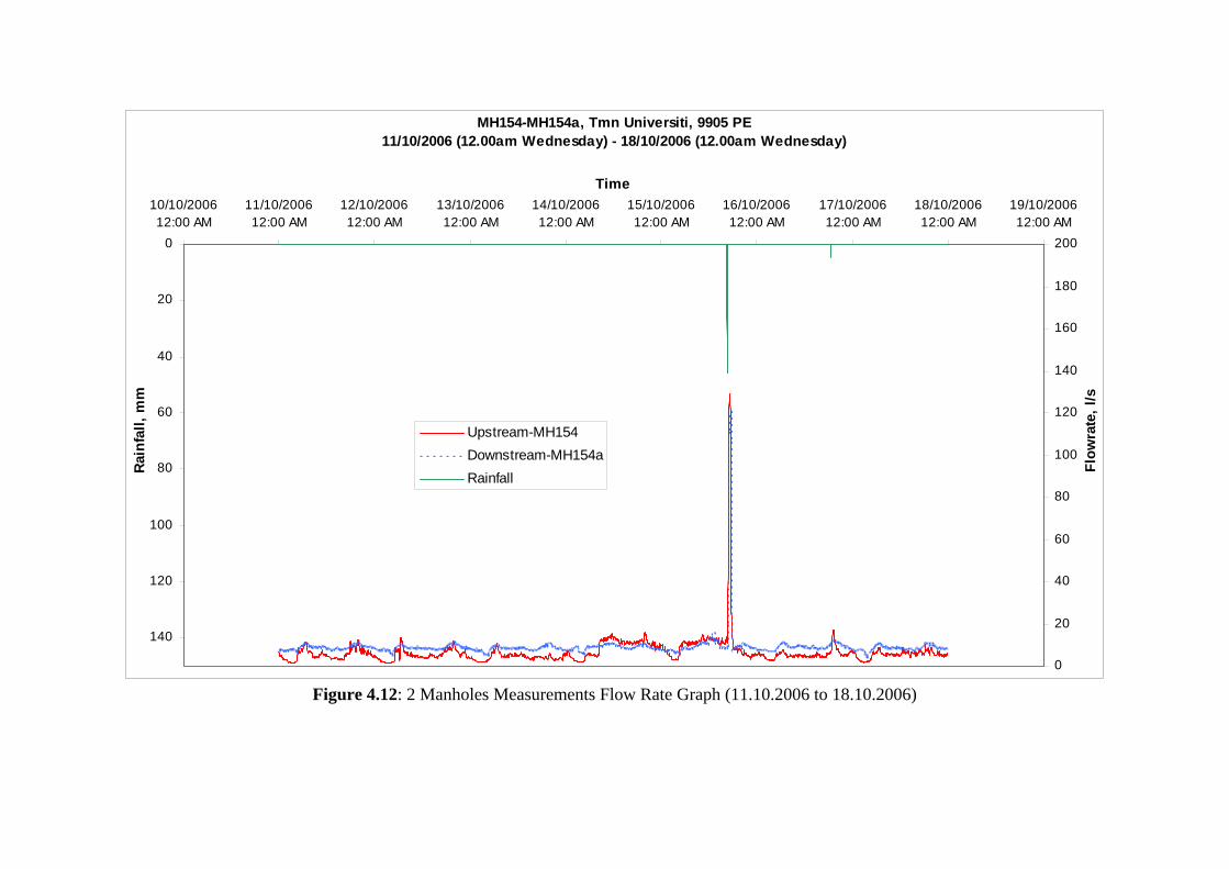
Figure 4.12: 2 Manholes Measurements Flow Rate Graph (11.10.2006 to 18.10.2006)
MH154-MH154a, Tmn Universiti, 9905 PE18/12/2006 (12.00pm Monday) - 25/12/2006 (12.00pm Monday)
0
10
20
30
40
50
18/12/200612:00 AM
19/12/200612:00 AM
20/12/200612:00 AM
21/12/200612:00 AM
22/12/200612:00 AM
23/12/200612:00 AM
24/12/200612:00 AM
25/12/200612:00 AM
26/12/200612:00 AM
Time
Rain
fall,
mm
0
20
40
60
80
100
120
140
160
180
200
Flow
rate
, l/sUpstream-MH154
Downstream-MH154aRainfall
Figure 4.13: 2 Manholes Measurements Flow Rate Graph (18.12.2006 to 25.12.2006)
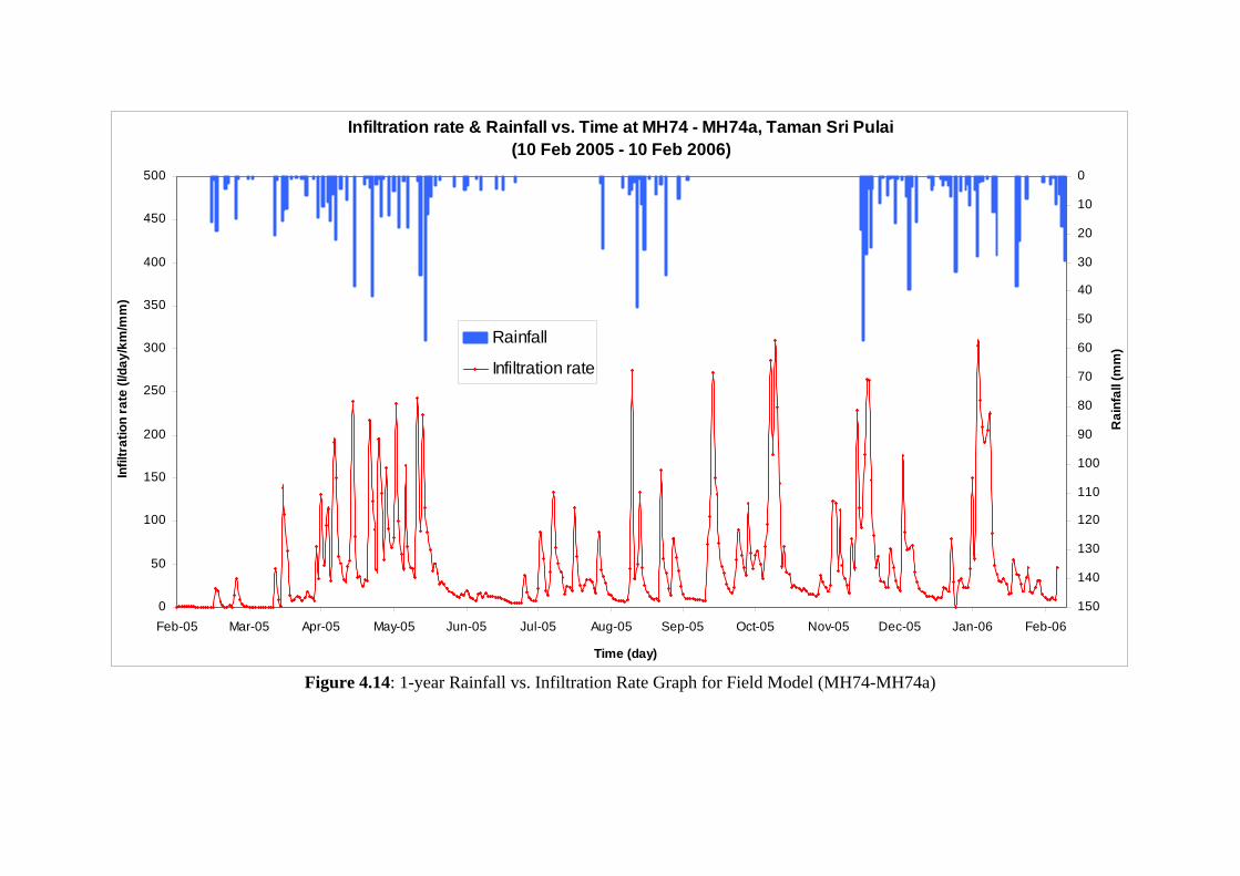
Infiltration rate & Rainfall vs. Time at MH74 - MH74a, Taman Sri Pulai(10 Feb 2005 - 10 Feb 2006)
0
50
100
150
200
250
300
350
400
450
500
Feb-05 Mar-05 Apr-05 May-05 Jun-05 Jul-05 Aug-05 Sep-05 Oct-05 Nov-05 Dec-05 Jan-06 Feb-06
Time (day)
Infil
trat
ion
rate
(l/d
ay/k
m/m
m)
0
10
20
30
40
50
60
70
80
90
100
110
120
130
140
150
Rai
nfal
l (m
m)
Rainfall
Infiltration rate
Figure 4.14: 1-year Rainfall vs. Infiltration Rate Graph for Field Model (MH74-MH74a)
CHAPTER 5
ANALYSIS AND DISCUSSION
5.1 Flow Characteristics Study
The study for the determination of flow characteristics is conducted in two residential areas of Skudai, Johor Bahru in the running sewer lines having different population equivalents. The first study is conducted on manhole MH11, Taman Sri Pulai residential area, Skudai, Johor. This line caters to a population equivalent of 1705. The second study is conducted on the manhole MH299 and MH154, Taman Universiti residential area, Skudai, Johor. This line caters to a population equivalent of 3456 and 9905. The flow meter is calibrated first in the Laboratory of Hydraulics & Hydrology, FKA, UTM, Skudai, Johor just to make sure that the equipment is working properly with minimum chances of error. The detail of the flow meter calibration is given in article 5.1.1. The details of the flow characteristics found during study on the two lines are discussed below: 5.1.1 Calibration of ISCO Area - Velocity Flow Meter
The calibration of the ISCO Area Velocity Flow Meter model 4250 is done in the laboratory of Hydraulics & Hydrology, Universiti Teknologi Malaysia. Two different sensors are used to measure the flow in the channel, velocity in the channel and depth of water level in the channel. The calibration is done on the Laminar/Turbulence Flow Apparatus by Plint & Partners, UK. The procedure for the determination of percent error, for different depths of flow, in the flow meter is described below:
1. Put the sensor in the channel and open the valve to start the flow of water in the channel after switching on the power supply.
2. Measure the initial depth in the channel as well as the width of the channel and input the same in the flow meter.
3. Find the differential head from the differential manometer attached with the apparatus.
4. With the help of this differential head find the flow in litres/second in the channel using the Manning’s graph.
5. Using the depth of flow and the width of channel to find the area of flow in the channel to find the velocity of flow in the channel.
6. Note the depth, velocity and flow through the area velocity flow meter and compare the results with the actual values found manually.
7. Hence the percentage error for the values. 8. Repeat the steps from step 3 to 7 by increasing the flow in the channel
slowly.
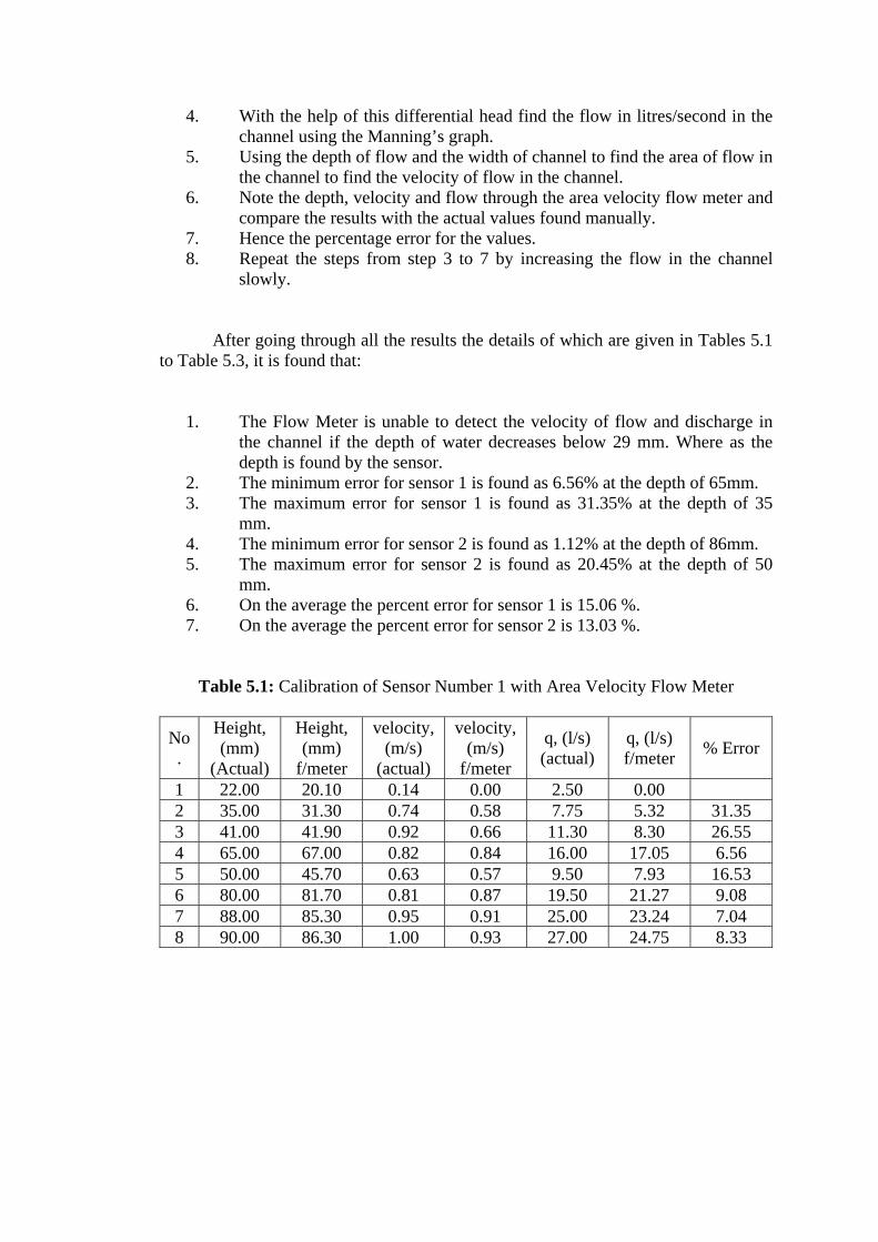
After going through all the results the details of which are given in Tables 5.1 to Table 5.3, it is found that:
1. The Flow Meter is unable to detect the velocity of flow and discharge in the channel if the depth of water decreases below 29 mm. Where as the depth is found by the sensor.
2. The minimum error for sensor 1 is found as 6.56% at the depth of 65mm. 3. The maximum error for sensor 1 is found as 31.35% at the depth of 35
mm. 4. The minimum error for sensor 2 is found as 1.12% at the depth of 86mm. 5. The maximum error for sensor 2 is found as 20.45% at the depth of 50
mm. 6. On the average the percent error for sensor 1 is 15.06 %. 7. On the average the percent error for sensor 2 is 13.03 %.
Table 5.1: Calibration of Sensor Number 1 with Area Velocity Flow Meter
No.
Height, (mm)
(Actual)
Height, (mm)
f/meter
velocity, (m/s)
(actual)
velocity, (m/s)
f/meter
q, (l/s) (actual)
q, (l/s) f/meter % Error
1 22.00 20.10 0.14 0.00 2.50 0.00 2 35.00 31.30 0.74 0.58 7.75 5.32 31.35 3 41.00 41.90 0.92 0.66 11.30 8.30 26.55 4 65.00 67.00 0.82 0.84 16.00 17.05 6.56 5 50.00 45.70 0.63 0.57 9.50 7.93 16.53 6 80.00 81.70 0.81 0.87 19.50 21.27 9.08 7 88.00 85.30 0.95 0.91 25.00 23.24 7.04 8 90.00 86.30 1.00 0.93 27.00 24.75 8.33
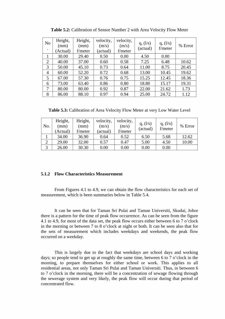
Table 5.2: Calibration of Sensor Number 2 with Area Velocity Flow Meter
No.
Height, (mm)
(Actual)
Height, (mm)
f/meter
velocity, (m/s)
(actual)
velocity, (m/s)
f/meter
q, (l/s) (actual)
q, (l/s) f/meter % Error
1 30.00 29.40 0.50 0.00 4.50 0.00 2 40.00 37.00 0.60 0.58 7.25 6.48 10.62 3 50.00 45.10 0.73 0.64 11.00 8.75 20.45 4 60.00 52.20 0.72 0.68 13.00 10.45 19.62 5 67.00 57.30 0.76 0.75 15.25 12.45 18.36 6 73.00 63.40 0.86 0.80 18.80 15.17 19.31 7 80.00 80.00 0.92 0.87 22.00 21.62 1.73 8 86.00 88.10 0.97 0.94 25.00 24.72 1.12
Table 5.3: Calibration of Area Velocity Flow Meter at very Low Water Level
No. Height, (mm)
(Actual)
Height, (mm)
f/meter
velocity, (m/s)
(actual)
velocity, (m/s)
f/meter
q, (l/s) (actual)
q, (l/s) f/meter % Error
1 34.00 36.90 0.64 0.52 6.50 5.68 12.62 2 29.00 32.00 0.57 0.47 5.00 4.50 10.00 3 26.00 30.30 0.00 0.00 0.00 0.00
5.1.2 Flow Characteristics Measurement
From Figures 4.1 to 4.9, we can obtain the flow characteristics for each set of measurement, which is been summaries below in Table 5.4.
It can be seen that for Taman Sri Pulai and Taman Universiti, Skudai, Johor there is a pattern for the time of peak flow occurrence. As can be seen from the figure 4.1 to 4.9, for most of the data set, the peak flow occurs either between 6 to 7 o’clock in the morning or between 7 to 8 o’clock at night or both. It can be seen also that for the sets of measurement which includes weekdays and weekends, the peak flow occurred on a weekday.
This is largely due to the fact that weekdays are school days and working
days; so people tend to get up at roughly the same time, between 6 to 7 o’clock in the morning, to prepare themselves for either school or work. This applies to all residential areas, not only Taman Sri Pulai and Taman Universiti. Thus, in between 6 to 7 o’clock in the morning, there will be a concentration of sewage flowing through the sewerage system and very likely, the peak flow will occur during that period of concentrated flow.
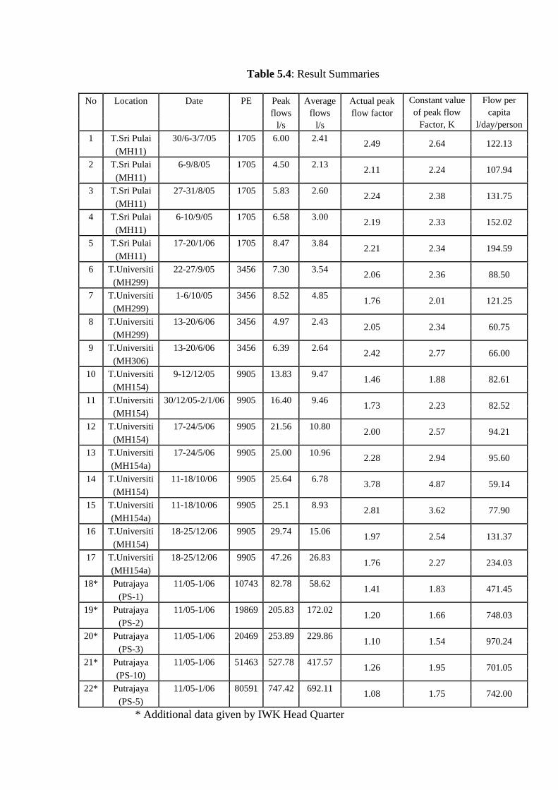
Table 5.4: Result Summaries
No Location Date PE Peak Average Actual peak Constant value Flow per flows flows flow factor of peak flow capita l/s l/s Factor, K l/day/person1 T.Sri Pulai 30/6-3/7/05 1705 6.00 2.41 (MH11)
2.49 2.64 122.13
2 T.Sri Pulai 6-9/8/05 1705 4.50 2.13 (MH11)
2.11 2.24 107.94
3 T.Sri Pulai 27-31/8/05 1705 5.83 2.60 (MH11)
2.24 2.38 131.75
4 T.Sri Pulai 6-10/9/05 1705 6.58 3.00 (MH11)
2.19 2.33 152.02
5 T.Sri Pulai 17-20/1/06 1705 8.47 3.84 (MH11)
2.21 2.34 194.59
6 T.Universiti 22-27/9/05 3456 7.30 3.54 (MH299)
2.06 2.36 88.50
7 T.Universiti 1-6/10/05 3456 8.52 4.85 (MH299)
1.76 2.01 121.25
8 T.Universiti 13-20/6/06 3456 4.97 2.43 (MH299)
2.05 2.34 60.75
9 T.Universiti 13-20/6/06 3456 6.39 2.64 (MH306)
2.42 2.77 66.00
10 T.Universiti 9-12/12/05 9905 13.83 9.47 (MH154)
1.46 1.88 82.61
11 T.Universiti 30/12/05-2/1/06 9905 16.40 9.46 (MH154)
1.73 2.23 82.52
12 T.Universiti 17-24/5/06 9905 21.56 10.80 (MH154)
2.00 2.57 94.21
13 T.Universiti 17-24/5/06 9905 25.00 10.96 (MH154a)
2.28 2.94 95.60
14 T.Universiti 11-18/10/06 9905 25.64 6.78 (MH154)
3.78 4.87 59.14
15 T.Universiti 11-18/10/06 9905 25.1 8.93 (MH154a)
2.81 3.62 77.90
16 T.Universiti 18-25/12/06 9905 29.74 15.06 (MH154)
1.97 2.54 131.37
17 T.Universiti 18-25/12/06 9905 47.26 26.83 (MH154a)
1.76 2.27 234.03
18* Putrajaya 11/05-1/06 10743 82.78 58.62 (PS-1)
1.41 1.83 471.45
19* Putrajaya 11/05-1/06 19869 205.83 172.02 (PS-2)
1.20 1.66 748.03
20* Putrajaya 11/05-1/06 20469 253.89 229.86 (PS-3)
1.10 1.54 970.24
21* Putrajaya 11/05-1/06 51463 527.78 417.57 (PS-10)
1.26 1.95 701.05
22* Putrajaya 11/05-1/06 80591 747.42 692.11 (PS-5)
1.08 1.75 742.00
* Additional data given by IWK Head Quarter

The same scene can be seen between 7 to 8 o’clock at night when people return home to freshen and clean themselves up after a long day at work or school in the afternoon session. When the bathrooms and toilets in most of the houses are used at roughly the same time between 7 to 8 o’clock at night, there will be a concentration of sewage flow in the sewerage system so there is a big chance of the peak flow occurring during that period of time. Of course, there will be anomalies like data set in certain figure where the peak flow occurs between 10 to 11 o’clock in the morning but that is to be expected in a research like this.
The average flow for Taman Sri Pulai is taken as the average of the Q average
for 1705 PE data, which is 2.8 litres/second. The minimum flow for all the measurements is 0.1 litres/second.
The average flow for Taman Universiti (MH299 and MH 154) is taken as the average of the Q average for 3456 PE and 9905 PE data, which is 3.37 litres/second and 12.29 litres/second. The minimum flow for all the measurements is 0.1 litres/second.
From Tables 5.4, it can be seen that Taman Universiti has bigger average flows and peak flows compared to Taman Sri Pulai. This is due to the fact that the population equivalent for the sewerage line in which we did our study is much bigger than the population equivalent for the sewerage line studied in Taman Sri Pulai.
5.1.3 Flow Per Capita Contribution
After determining the flow characteristics for each of the flow measurement, the per capita flow contribution can be obtain for each measurement set by dividing the Q average for each set of measurement with the population equivalent of the study area, which is 1705, 3456 and 9905. The results are tabled below in Table 5.4.
From Table 5.4, the flow per capita obtained for each set of measurement is significantly lower than the design flow per capita of 0.225m3/day-person suggested in MS1228:1991. The average flow per capita for Taman Sri Pulai sets of measurement is 0.142 m3/day-person, which is 37% lower than the design flow per capita of 0.225 m3/day-person recommended in MS1228:1991.
The average flow per capita from the Taman Universiti data sets is 0.1 m3/day-
person, 56% lower than the 0.225 m3/day-person recommended in MS1228:1991.
Thus, it can be deduced from the actual flow per capita results obtained that the current sewerage design is more than sufficient to cater for the daily sewage disposal needs of the residents in Taman Sri Pulai and Taman Universiti. 5.1.4 Peak Flow Factor
Next after obtaining the actual flow per capita contribution of the study area,
the peak flow factor, can be calculated from Equation 3.4 by rearranging the parameters in the equation. The actual peak flow factor value calculated using actual flow per capita contribution is compared with the design peak flow factor value calculated using MS1228:1991 recommended equation. The results of peak flow factor value calculation is in Table 5.4 and note that the current practice in design of sewerage systems uses peak flow factor equation of 4.7p-0.11.
By using the actual flow per capita calculated for each set of data, the peak flow factor value for each data set is found to be less than the value of the design peak flow factor recommended by MS1228:1991 and used in current design practice. The average peak flow factor value calculated using actual flow per capita for Taman Sri Pulai sets of measurement is 2.25. This is 49% lower than the design peak flow factor value used in current design practice.
As for Taman Universiti, the actual peak flow factor values obtained by using the actual flow per capita calculated is also less than the design peak flow factor. The average peak flow factor value for 3456 PE site calculated using actual flow per capita contribution is 2.07, which is 50% lower than the design peak flow factor value used in current sewerage system design practice. And the average peak flow factor value for 9905 PE site calculated using actual flow per capita contribution is 2.32, which is 39% lower than the design peak flow factor value used in current sewerage system design practice.
This means that the current sewerage system design in Malaysia is over design
or in another word the design peak flow factor recommended by MS1228:1991 is too high for designing sewerages system in this country.
If the actual peak flow factor is calculated using the MS1228:1991
recommended flow per capita contribution of 0.225m3/day-person, the value that were obtain is even lower than the actual peak flow factor result that were calculated using the actual flow per capita contribution measured from the field experiment.
In this study we are looking for the optimum design criterion for sewerage systems in a tropical climate. Since the peak flow factor is used in conjunction with the average flow and population equivalent to obtain the estimated peak flow to be used in the design of a sewerage system, it is the design criterion in Equation 3.4 that is looked into in this study.
From Equation 3.4, we can see that there is a proportional relationship
between peak flow factor value and the Q peak. The bigger the peak flow factor value used, the bigger the Q peak value will be get. A higher value of Q peak used in sewerage system designs will result in bigger sizes of sewerage pipes needed since velocity of sewage flow is limited to a particular range only. This translates to higher cost of material and works for construction of the sewerage system. All this is can be avoided because from the actual results obtained from site, the peak flow factor value to be used need not be as high as recommended.
In view of the peak flow factor value obtained from this study in Taman Sri
Pulai and Taman Universiti, it can be said that the sewerage system in this two residential areas is over designed since it was designed using the MS1228:1991 recommended peak flow factor value of 4.7p-0.11 whereas the actual peak flow factor value can range from 1.46 to 3.78, depending on the flow per capita used during the design process.
The comparison of results and analysis of this study conducted in Taman Sri Pulai and Taman Universiti shows that the sewerage system in this two residential areas is indeed designed for more than necessary and the parties involved in constructing the sewerage system could have avoided the extra cost if they were to use a smaller but suitable peak flow factor value in the calculation for peak flow to design the sewerage system.
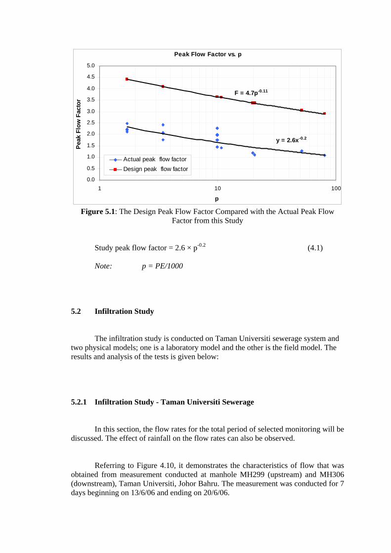
The results of the actual peak flow factor and design peak flow factor value that was obtained through analysis was plotted again ‘p’ (p = PE/1000) value using a semi log graph. And then from the plotted graph, a new power equation of peak flow factor for designing sewerage system was produce. Figure 5.1 demonstrates the actual peak flow factor equation is different from the design peak flow factor equation currently used in sewerage system design.
It obviously illustrate that both of the graph lines are parallel as depicted in Figure 5.1. So, from this study, the design peak flow factor equation used by Malaysian Standard, MS 1228:1991 that is 4.7 × p-0.11 can be replaced with a new equation as equation 4.1 below. This equation hopefully can assist in designing and developing a future vitrified clay pipe sewerage system.
Peak Flow Factor vs. p
F = 4.7p-0.11
y = 2.6x-0.2
0.0
0.5
1.0
1.5
2.0
2.5
3.0
3.5
4.0
4.5
5.0
1 10 100
p
Pea
k Fl
ow F
acto
r
Actual peak flow factorDesign peak flow factor
Figure 5.1: The Design Peak Flow Factor Compared with the Actual Peak Flow
Factor from this Study
Study peak flow factor = 2.6 × p-0.2 (4.1)
Note: p = PE/1000 5.2 Infiltration Study
The infiltration study is conducted on Taman Universiti sewerage system and two physical models; one is a laboratory model and the other is the field model. The results and analysis of the tests is given below: 5.2.1 Infiltration Study - Taman Universiti Sewerage
In this section, the flow rates for the total period of selected monitoring will be discussed. The effect of rainfall on the flow rates can also be observed.
Referring to Figure 4.10, it demonstrates the characteristics of flow that was obtained from measurement conducted at manhole MH299 (upstream) and MH306 (downstream), Taman Universiti, Johor Bahru. The measurement was conducted for 7 days beginning on 13/6/06 and ending on 20/6/06.
In Figure 4.10 a drastic increase in flow is observed on the 13/6/06. The rain intensity on that day is recorded as 14.7 mm. This contributed to the highest flow recorded, which is 13.3 l/s. Consequently, this difference and increment illustrates prove that there is an inflow and infiltration occurrence in the sewerage pipe during rain fall. Infiltration can also be seen to occur a lot as the value of upstream flow rate is lower than the downstream flow rate (Q out > Q in). However, there were also instances when (Q out < Q in), or the downstream flow rate is lesser than that of the upstream. During such instances, leakage is happening.
Referring to Figure 4.11, it demonstrates the characteristics of flow that was obtained from measurement conducted at manhole MH154 (upstream) and MH154a (downstream), Taman Universiti, Johor Bahru. The measurement was conducted for 7 days beginning on 17/5/06 and ending on 24/5/06.
In Figure 4.11 a drastic increase in flow is observed on the 19/5/06. The rain intensity on that day is recorded as 20.9 mm. This contributed to the highest flow recorded, which is 80.53 l/s. Consequently, this difference and increment illustrates prove that there is an inflow and infiltration occurrence in the sewerage pipe during rain fall. Infiltration can also be seen to occur a lot as the value of upstream flow rate is lower than the downstream flow rate (Q out > Q in). However, there were also instances when (Q out < Q in), or the downstream flow rate is lesser than that of the upstream. During such instances, leakage is happening.
Referring to Figure 4.12, the characteristics of flow that was obtained from measurement conducted at the same sewer line is shown. The measurement was conducted for 7 days beginning on 11/10/06 and ending on 18/10/06.
In Figure 4.12 a drastic increase in flow is observed on the 15/10/06. The rain intensity on that day is recorded as 45.72 mm. This contributed to the highest flow recorded, which is 129.4 l/s. Consequently, this difference and increment illustrates prove that there is an inflow and infiltration occurrence in the sewerage pipe during rain fall. Infiltration can also be seen to occur a lot as the value of upstream flow rate is lower than the downstream flow rate (Q out > Q in). However, there were also instances when (Q out < Q in), or the downstream flow rate is lesser than that of the upstream. During such instances, leakage is happening.
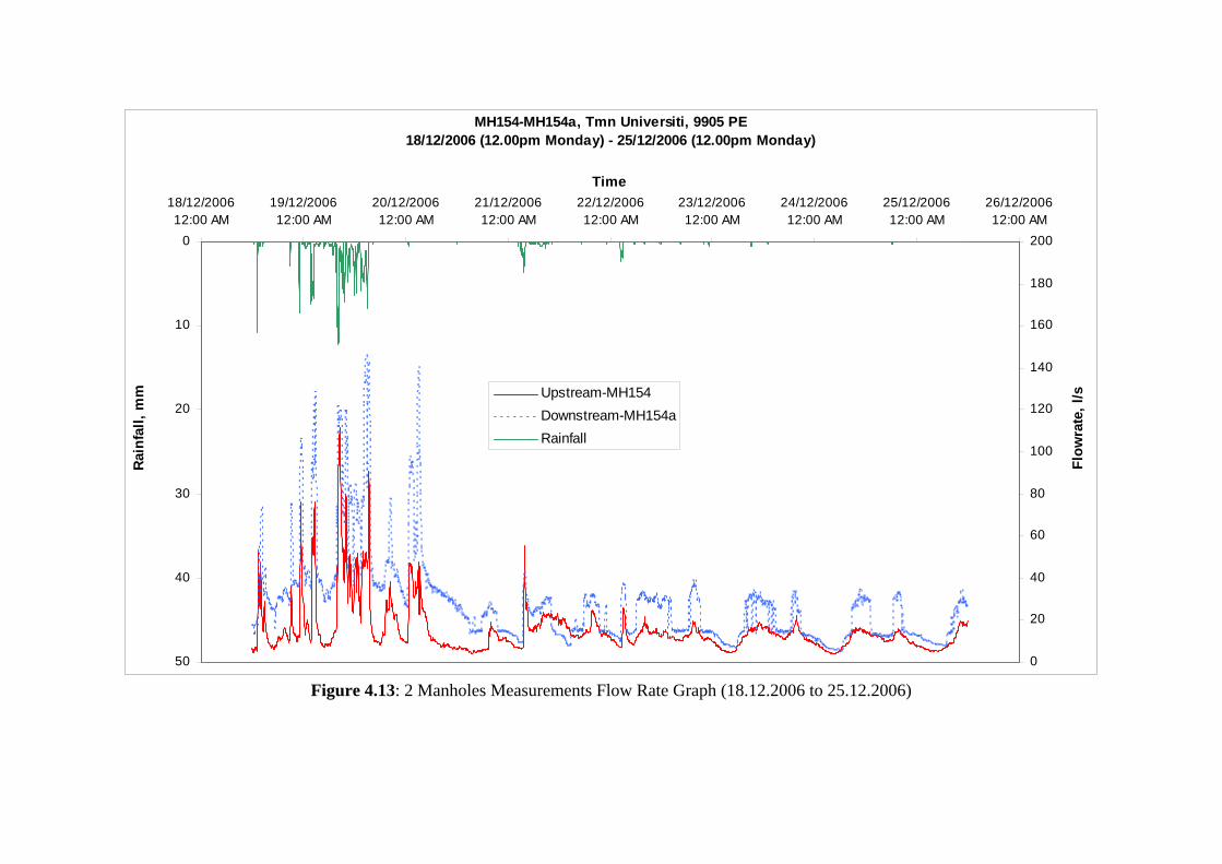
Referring to Figure 4.13, the characteristics of flow that was obtained from measurement conducted at the same sewer line is shown. The measurement was conducted for 7 days beginning on 18/12/06 and ending on 25/12/06.
Just as the previous monitoring, it is observed that the flow rate is vastly influenced by the rainfall. Here the rain intensity was very much higher and the recorded value for the 19/12/06 alone was 282.6 mm. Heavy rain was experienced on other days as well. Due to this, the flow rates recorded showed peaks which tallied
with the occurrence of rain. The highest flow rate recorded on that day is 146.2 l/s. The infiltration and leakage can be seen much clearer in this graph as the flow rates are very unstable and the scale of the graph allows for easier observance on the differences in flow that has occurred. 5.2.1.1 Infiltration Analysis
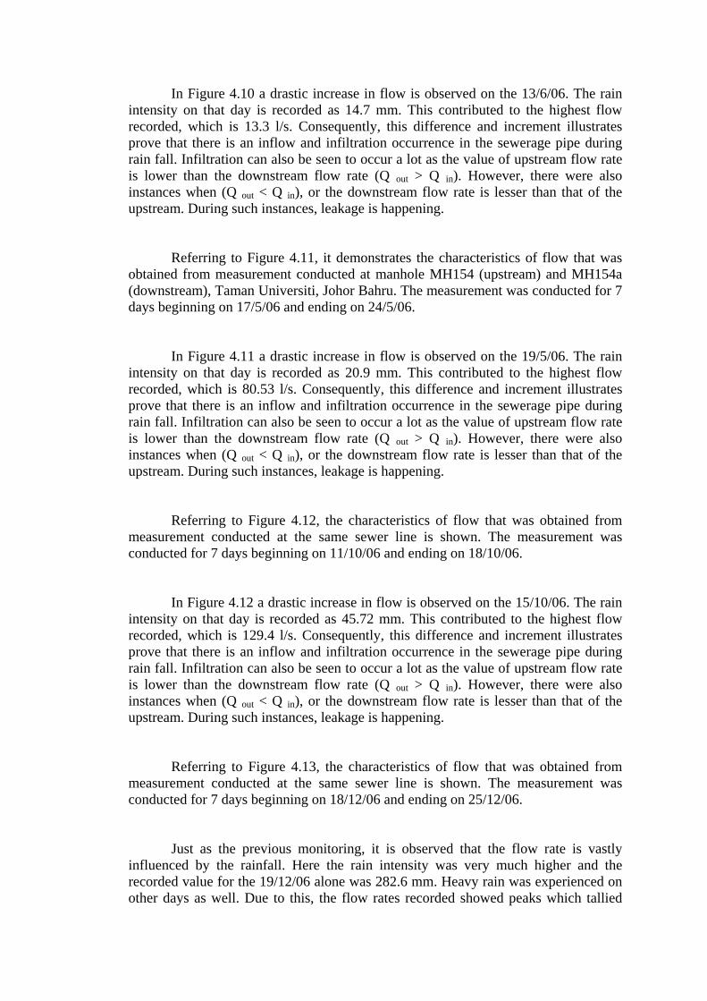
In Figure 5.2, the infiltration that occurred between 13.6.2007 to 20.6.2007 is shown. The highest rate of infiltration recorded is 4.47 m3/day/km-length/mm-diameter. There was not much infiltration due to less rainfall occurs that week. What can be noticed is the rapid increase of infiltration that occurs after rain. The recommended rate by MS1228:1991 and Hammer & Hammer (2004), is 0.05 m3/day/km-length/mm-diameter. The difference observed is 8840% higher.
Inflow & Infiltration at MH299-MH306, Tmn Universiti, 3456 PE13/6/2006 (12.00am Tuesday) - 20/6/2006 (12.00am Tuesday)
0.00
5.00
10.00
15.00
20.00
25.00
30.00
12/06/200612:00 AM
13/06/200612:00 AM
14/06/200612:00 AM
15/06/200612:00 AM
16/06/200612:00 AM
17/06/200612:00 AM
18/06/200612:00 AM
19/06/200612:00 AM
20/06/200612:00 AM
Time
Rain
fall,
mm
0.00
1.00
2.00
3.00
4.00
5.00
6.00
7.00
8.00
9.00
10.00
Inflo
w &
Infil
tratio
n,
m3/
day/
km/m
m
rainfallinflow & infiltration
Figure 5.2: Infiltration against Rainfall Graph (13.6.2006 to 20.6.2006)
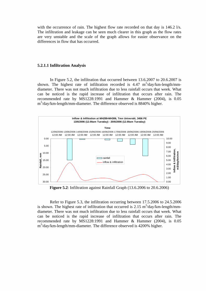
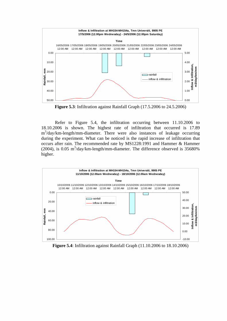
Refer to Figure 5.3, the infiltration occurring between 17.5.2006 to 24.5.2006 is shown. The highest rate of infiltration that occurred is 2.15 m3/day/km-length/mm-diameter. There was not much infiltration due to less rainfall occurs that week. What can be noticed is the rapid increase of infiltration that occurs after rain. The recommended rate by MS1228:1991 and Hammer & Hammer (2004), is 0.05 m3/day/km-length/mm-diameter. The difference observed is 4200% higher.
Inflow & Infiltration at MH154-MH154a, Tmn Universiti, 9905 PE 17/5/2006 (12.00pm Wednesday) - 24/5/2006 (12.00pm Saturday)
0.00
10.00
20.00
30.00
40.00
50.00
16/05/200612:00 AM
17/05/200612:00 AM
18/05/200612:00 AM
19/05/200612:00 AM
20/05/200612:00 AM
21/05/200612:00 AM
22/05/200612:00 AM
23/05/200612:00 AM
24/05/200612:00 AM
TimeR
ainf
all,
mm
0.00
1.00
2.00
3.00
4.00
5.00
Inflo
w &
Infil
tratio
n,
m3/
day/
km/m
m
rainfallinflow & infiltration
Figure 5.3: Infiltration against Rainfall Graph (17.5.2006 to 24.5.2006)
Refer to Figure 5.4, the infiltration occurring between 11.10.2006 to 18.10.2006 is shown. The highest rate of infiltration that occurred is 17.89 m3/day/km-length/mm-diameter. There were also instances of leakage occurring during the experiment. What can be noticed is the rapid increase of infiltration that occurs after rain. The recommended rate by MS1228:1991 and Hammer & Hammer (2004), is 0.05 m3/day/km-length/mm-diameter. The difference observed is 35680% higher.
Inflow & Infiltration at MH154-MH154a, Tmn Universiti, 9905 PE11/10/2006 (12.00am Wednesday) - 18/10/2006 (12.00am Wednesday)
0.00
20.00
40.00
60.00
80.00
100.00
10/10/200612:00 AM
11/10/200612:00 AM
12/10/200612:00 AM
13/10/200612:00 AM
14/10/200612:00 AM
15/10/200612:00 AM
16/10/200612:00 AM
17/10/200612:00 AM
18/10/200612:00 AM
Time
Rain
fall,
mm
-10.00
0.00
10.00
20.00
30.00
40.00
50.00In
flow
& In
filtr
atio
n,
m3/
day/
km/m
m
rainfallinflow & infiltration
Figure 5.4: Infiltration against Rainfall Graph (11.10.2006 to 18.10.2006)
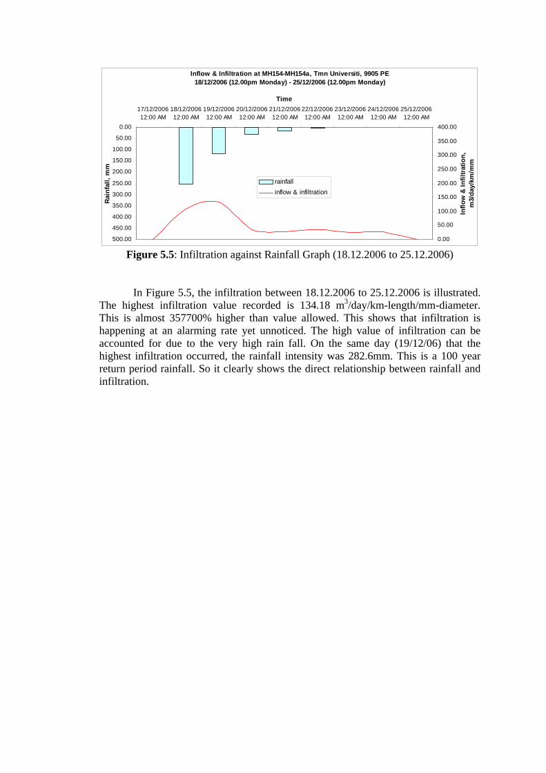
Inflow & Infiltration at MH154-MH154a, Tmn Universiti, 9905 PE18/12/2006 (12.00pm Monday) - 25/12/2006 (12.00pm Monday)
0.00
50.00
100.00
150.00
200.00
250.00
300.00
350.00
400.00
450.00
500.00
17/12/200612:00 AM
18/12/200612:00 AM
19/12/200612:00 AM
20/12/200612:00 AM
21/12/200612:00 AM
22/12/200612:00 AM
23/12/200612:00 AM
24/12/200612:00 AM
25/12/200612:00 AM
TimeR
ainf
all,
mm
0.00
50.00
100.00
150.00
200.00
250.00
300.00
350.00
400.00
Inflo
w &
Infil
trat
ion,
m
3/da
y/km
/mm
rainfallinflow & infiltration
Figure 5.5: Infiltration against Rainfall Graph (18.12.2006 to 25.12.2006)
In Figure 5.5, the infiltration between 18.12.2006 to 25.12.2006 is illustrated. The highest infiltration value recorded is 134.18 m3/day/km-length/mm-diameter. This is almost 357700% higher than value allowed. This shows that infiltration is happening at an alarming rate yet unnoticed. The high value of infiltration can be accounted for due to the very high rain fall. On the same day (19/12/06) that the highest infiltration occurred, the rainfall intensity was 282.6mm. This is a 100 year return period rainfall. So it clearly shows the direct relationship between rainfall and infiltration.
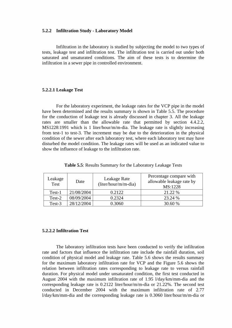
5.2.2 Infiltration Study - Laboratory Model
Infiltration in the laboratory is studied by subjecting the model to two types of tests, leakage test and infiltration test. The infiltration test is carried out under both saturated and unsaturated conditions. The aim of these tests is to determine the infiltration in a sewer pipe in controlled environment. 5.2.2.1 Leakage Test
For the laboratory experiment, the leakage rates for the VCP pipe in the model have been determined and the results summary is shown in Table 5.5. The procedure for the conduction of leakage test is already discussed in chapter 3. All the leakage rates are smaller than the allowable rate that permitted by section 4.4.2.2, MS1228:1991 which is 1 liter/hour/m/m-dia. The leakage rate is slightly increasing from test-1 to test-3. The increment may be due to the deterioration in the physical condition of the sewer after each laboratory test, where each laboratory test may have disturbed the model condition. The leakage rates will be used as an indicated value to show the influence of leakage to the infiltration rate.
Table 5.5: Results Summary for the Laboratory Leakage Tests
Leakage Test Date Leakage Rate
(liter/hour/m/m-dia)
Percentage compare with allowable leakage rate by
MS:1228 Test-1 21/08/2004 0.2122 21.22 % Test-2 08/09/2004 0.2324 23.24 % Test-3 28/12/2004 0.3060 30.60 %
5.2.2.2 Infiltration Test
The laboratory infiltration tests have been conducted to verify the infiltration rate and factors that influence the infiltration rate include the rainfall duration, soil condition of physical model and leakage rate. Table 5.6 shows the results summary for the maximum laboratory infiltration rate for VCP and the Figure 5.6 shows the relation between infiltration rates corresponding to leakage rate to versus rainfall duration. For physical model under unsaturated condition, the first test conducted in August 2004 with the maximum infiltration rate of 1.95 l/day/km/mm-dia and the corresponding leakage rate is 0.2122 liter/hour/m/m-dia or 21.22%. The second test conducted in December 2004 with the maximum infiltration rate of 2.77 l/day/km/mm-dia and the corresponding leakage rate is 0.3060 liter/hour/m/m-dia or
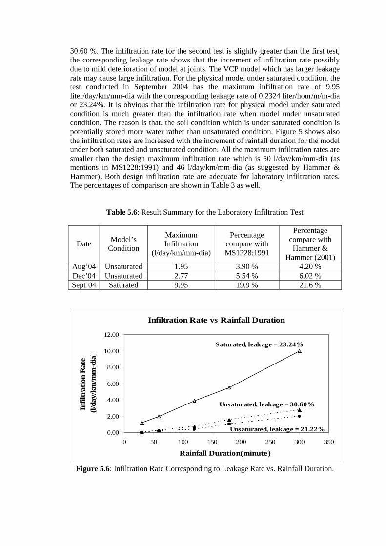
30.60 %. The infiltration rate for the second test is slightly greater than the first test, the corresponding leakage rate shows that the increment of infiltration rate possibly due to mild deterioration of model at joints. The VCP model which has larger leakage rate may cause large infiltration. For the physical model under saturated condition, the test conducted in September 2004 has the maximum infiltration rate of 9.95 liter/day/km/mm-dia with the corresponding leakage rate of 0.2324 liter/hour/m/m-dia or 23.24%. It is obvious that the infiltration rate for physical model under saturated condition is much greater than the infiltration rate when model under unsaturated condition. The reason is that, the soil condition which is under saturated condition is potentially stored more water rather than unsaturated condition. Figure 5 shows also the infiltration rates are increased with the increment of rainfall duration for the model under both saturated and unsaturated condition. All the maximum infiltration rates are smaller than the design maximum infiltration rate which is 50 l/day/km/mm-dia (as mentions in MS1228:1991) and 46 l/day/km/mm-dia (as suggested by Hammer & Hammer). Both design infiltration rate are adequate for laboratory infiltration rates. The percentages of comparison are shown in Table 3 as well.
Table 5.6: Result Summary for the Laboratory Infiltration Test
Date Model’s Condition
Maximum Infiltration
(l/day/km/mm-dia)
Percentage compare with MS1228:1991
Percentage compare with Hammer &
Hammer (2001) Aug’04 Unsaturated 1.95 3.90 % 4.20 % Dec’04 Unsaturated 2.77 5.54 % 6.02 % Sept’04 Saturated 9.95 19.9 % 21.6 %
Infiltration Rate vs Rainfall Duration
0.00
2.00
4.00
6.00
8.00
10.00
12.00
0 50 100 150 200 250 300 350
Rainfall Duration(minute)
Infil
trat
ion
Rat
e (l
/day
/km
/mm
-dia
)
Saturated, leakage = 23.24%
Unsaturated, leakage = 30.60%
Unsaturated, leakage = 21.22%
Figure 5.6: Infiltration Rate Corresponding to Leakage Rate vs. Rainfall Duration.
5.2.3 Infiltration Study - Field Model
The infiltration study was conducted on the field test model which is an abandoned sewer section between manholes MH74 and MH74a. The data was collected continuously for one year starting from February 2005 and up to February 2006. The details of the infiltrated water collected daily in liters/day and the corresponding infiltration rate in liters/day/km-length/mm-diameter is given in Appendix - A. The one year data is include both wet and dry periods. The rainfall volume for the same 24-hour period is also measured with the help of automatic rain gauge measuring rainfall volume every five minutes of interval. 5.2.3.1 Infiltration Measurement
For infiltration measurement, Figures 4.14 shows the infiltration rate versus
rainfall for one year that the infiltration rate at the abandoned sewer line of MH74-MH74a is measured.
As can be seen from the graphs in Figures 4.14, whenever there is a significant
rainfall (the blue bars extending downwards) on a particular day, the infiltration rate will increase for that day, the graph line forming a peak. In some cases, the peaks for the infiltration graph line will appear a few days after a heavy rainfall. This is usually the case when it rains after a period of dryness. The rain will take time to seep through the dry soil to infiltrate into the abandoned sewer.
Most of the time, the infiltration rate will be below 50 litres/day/kilometre-
length/milimetre-diametre as recommended by MS1228:1991 when there is no rain or little rain (below 10mm) unless the rain happens suddenly after a period of dryness.
From Figure 4.14, it can be see that the highest infiltration rate, 310.19
litres/day/kilometre-length/milimetre-diametre occurred on 16.10.2005. This rate is over six times that of the allowable infiltration rate 50 litres/day/kilometre-length/milimetre-diametre stated in MS1228:1991.
Out of the 365 days, 100 days or approximately 27.4% of the days
experienced infiltration rate exceeding the recommended rate by MS1228:1991 as well as Hammer & Hammer (2004), which is 50 litres/day/kilometre-length/milimetre-diametre and 46 litres/day/kilometre-length/milimetre-diametre respectively.

As can be seen from Figure 4.14, the infiltration rate of a sewer line increases with the passing of time. When infiltration rate measurement works at the abandoned sewer line MH74-MH74a started on the 10th of February 2005, the rate of infiltration did not exceed 50 litres/day/kilometre-length/milimetre-diametre for six consecutive weeks because the sewer line was newly sealed with concrete. But after six weeks, infiltration rates exceeding 50 litres/day/kilometre-length/milimetre-diametre started to appear, the values growing ever higher whenever subsequent heavy rainfall occurred.
The graph in Figure 4.14 can be divided into two main periods, the dry period
and the wet period. Dry period is a period of a few days where there is little or no rainfall while wet period constitutes duration of days where there is heavy rainfall or consecutive rainfalls. By looking at Figure 4.14, we can see that infiltration rate is more significant during wet periods. Therefore, wet periods contribute more infiltration compared to dry periods.

CHAPTER 6
CONCLUSIONS AND RECOMMENDATIONS
6.1 Conclusion
After performing the study on Taman Sri Pulai and Taman Universiti, gathering as well as analyzing all the data, several conclusions can be gleaned from the result and analysis.
As can be seen that there are two periods of time in a day when hourly peak
flow is likely to occur, that is between 6am to 7am in the morning and between 7pm to 8pm at night. Also, the daily peak flow will fall on a weekday. These phenomena can be explained by the lifestyle of the residents at Taman Sri Pulai and Taman Universiti, which is largely made up of working adults and schooling children.
The average flow per capita contribution at Taman Sri Pulai and Taman
Universiti is lower than the design flow per capita used during the design of the sewerage system (0.225 m3/day-person). So it can be said that the current sewerage system at Taman Sri Pulai and Taman Universiti is adequate to support the sewage generated by the residents there.
From this analysis, it can be see that the peak flow factor recommended by
MS1228:1991 and used in current practice design is in fact very much bigger than necessary. Thus can be deduced that the peak flow factor equation used to get the peak flow in sewerage systems design is bigger than necessary, which will lead to unnecessary cost in material and labour.
From this study in Taman Sri Pulai and Taman Universiti, the peak flow factor
value obtained in each study is lower than the value used in current sewerage system design practice. The conclusion for this is there may be a need to review the whole equation used in sewerage system design practice, including the peak flow factor, the flow per capita contribution assumed as well as the hyper scripted –0.11 value for the population equivalent in thousands.
The infiltration measurement at the abandoned sewer line of MH74-MH74a in Taman Sri Pulai show and explain us whenever it rains, the infiltration rate for that day or for a few days after that will rise sharply compared to the previous date’s infiltration rate. It may thus be concluded that there is tremendous amount of extraneous water that seeps into the sewerage system as inflow/infiltration. Also it can be concluded that there is a proportional relationship between rainfall and infiltration rate in sewerage systems and that wet periods contribute significantly more infiltration into sewerage systems than dry periods. This is evident from the results of the study conducted on the field test model. Infiltration as high as 310 liters/day/km-length/mm-diameter has been found on the October 2005, which is much higher than the limit as given by Malaysian Standard MS1228:1991 which is 50 liters/day/km-length/mm-diameter and also much higher than the value given by Hammer & Hammer (2001) which is 46 liters/day/km-length/mm-diameter. This shows the effect of the rainfall on the infiltration in the sewers. During the dry period how ever the infiltration is with in the design limits as given by Malaysian Standard MS1228:1991 and also the value given by Hammer & Hammer (2001).
The test conducted on the laboratory model show a very encouraging picture. There were two type of tests conducted to measure the infiltration in a VCP sewer in the controlled environment. All the results of the leakage and infiltration tests show that the leakage and infiltration rate are with in the limits prescribed by Malaysian Standard MS1228:1991. This shows that with proper supervision during the construction period we can reduce the amount of infiltration in our sewerage system and indirectly reduce the load on our treatment plants. Therefore the workmanship during the construction process may be improved so that the undue pressure on the treatment plants during the wet periods may be removed. 6.2 Recommendations
These are a few of the recommendations suggested to improve on this study as well as similar future studies by having more comprehensive data and analysis.
i) Recount and reconfirm the population equivalent (PE) of the study area ii) Usage of 2 flowmeters in a suitable stretch of sewer line, one in the
upstream manhole and the other in the downstream manhole to register the amount of infiltration into the stretch of sewer line. This data is invaluable because it represents the actual infiltration rate happening in sewerage systems in Malaysia.
iii) Studies should be carried out in sewer lines catering to other different population equivalent so as to have data from sewerage lines with different population equivalent.

iv) All inflow and infiltration studies should be accompanied by the determination of the groundwater table level as well as the characteristics of the soil surrounding the sewer pipes.
v) Smoke testing can be conducted in sewer lines suspected of leakage to detect the exact location of leakage.
REFERENCES American Society of Civil Engineers (1982). Gravity Sanitary Sewer Design and
Construction. WPCF-Manuals Of Practice-No. FD-5.
Cheah Sau Wei (2002). Kajian Aliran Masuk Dan Penyusupan Dalam Sistem Pembetungan Di Taman Skudai Baru Dan Bandar Sri Alam Johor Bahru. Universiti Teknologi Malaysia : Thesis, B.Sc.
Hammer, M. J. and Hammer, M.J. Jr. (2004). Water and Wastewater Technology. 5th Edition. Pearson Prentice Hall
Ho Jenn Shing (2002). Kajian Aliran Masuk Dan Penyusupan Dalam Sistem Pembetungan Di Taman Sri Pulai Dan Taman Timor Johor Bahru. Universiti Teknologi Malaysia : Thesis, B.Sc.
Kamran (2005). Evaluation Of Inflow/Infiltration And Flow Characteristics For Design Of Sanitary Sewers In Skudai, Johor Bahru. Universiti Teknologi Malaysia : Thesis, M.Sc.
Kek Meng Liang (1999). Aliran Masuk Dan Penyusupan Dalam Sistem Pembetungan. Universiti Teknologi Malaysia : Thesis, B.Sc.
Liu, C. and Evett, J. B. (2005). Soils and Foundations. SI Edition. Pearson Prentice Hall.
Malaysian Standard (1991). Code of Practice for Design and Installation of Sewerage Systems. Malaysia:(MS 1228)
Mays, L. W. (2001). Stormwater Collection Systems Design Handbook. McGraw-Hill Mok Hun Yew (2005). Kajian Penyusupan Dan Kebocoran Bagi Paip Pembetung
VCP Dalam Sistem Pembetungan. Universiti Teknologi Malaysia : Thesis, B.Sc.
Ngoi Si Cheng (2003). Kajian Penyusupan Dalam Sistem Pembetung Di Johor Bahru. Universiti Teknologi Malaysia : Thesis, B.Sc.
Norhan Abdul Rahman (2003). Research Collaboration Between Indah Water Konsortium Sdn. Bhd. and Universiti Teknologi Malaysia Final Report Inflow & Infiltration In Sewerage Systems. Faculty of Civil Engineering, Universiti Teknologi Malaysia.

Novotny V., Imhoff, K. R., Olthof, M., Krenkel, P. A., (1989), Karl Imhoff’s Handbook Of Urban Drainage And Wastewater Disposal. John Wiley & Sons,
Onn bin Abdul Rani (2000). Kajian Aliran Masuk Dan Penyusupan Di Dalam Sistem Pembetungan. Universiti Teknologi Malaysia : Thesis, B.Sc.
Stenis, J. (2004). Industrial Management Models with Emphasis Construction Waste. Lund Institute of Technology : Doctoral Thesis.
Teh Woan Jin (2001). Kajian Tapak Dan Model Penyusupan Dan Aliran Dalam Sistem Pembetungan Di Taman Sri Pulai Johor Bahru. Universiti Teknologi Malaysia : Thesis, B. Sc.
Terzaghi, K., R. B. Peck, and G. Mesri (1996), Soil Mechanics in Engineering Practice, 3rd ed., John Wiley & Sons, Inc., New York.
Viessman W. Jr., Hammer M. J. (1985). Water Supply and Pollution Control. New York : Harper & Row, Publishers.
White, J. B. (1970). The Design of Sewers and Sewage Treatment Works. London : Edward Arnold (Publishers) Ltd.Inc.
Yusof Sukarti (2004). Kesan Aliran Masuk Dan Penyusupan Terhadap Sistem Pembetung Di Beberapa Kawasan Taman Perumahan Di Johor Bahru. Universiti Teknologi Malaysia : Thesis, M.Sc.
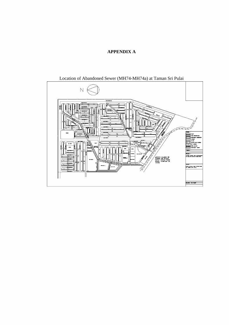
APPENDIX A
Location of Abandoned Sewer (MH74-MH74a) at Taman Sri Pulai
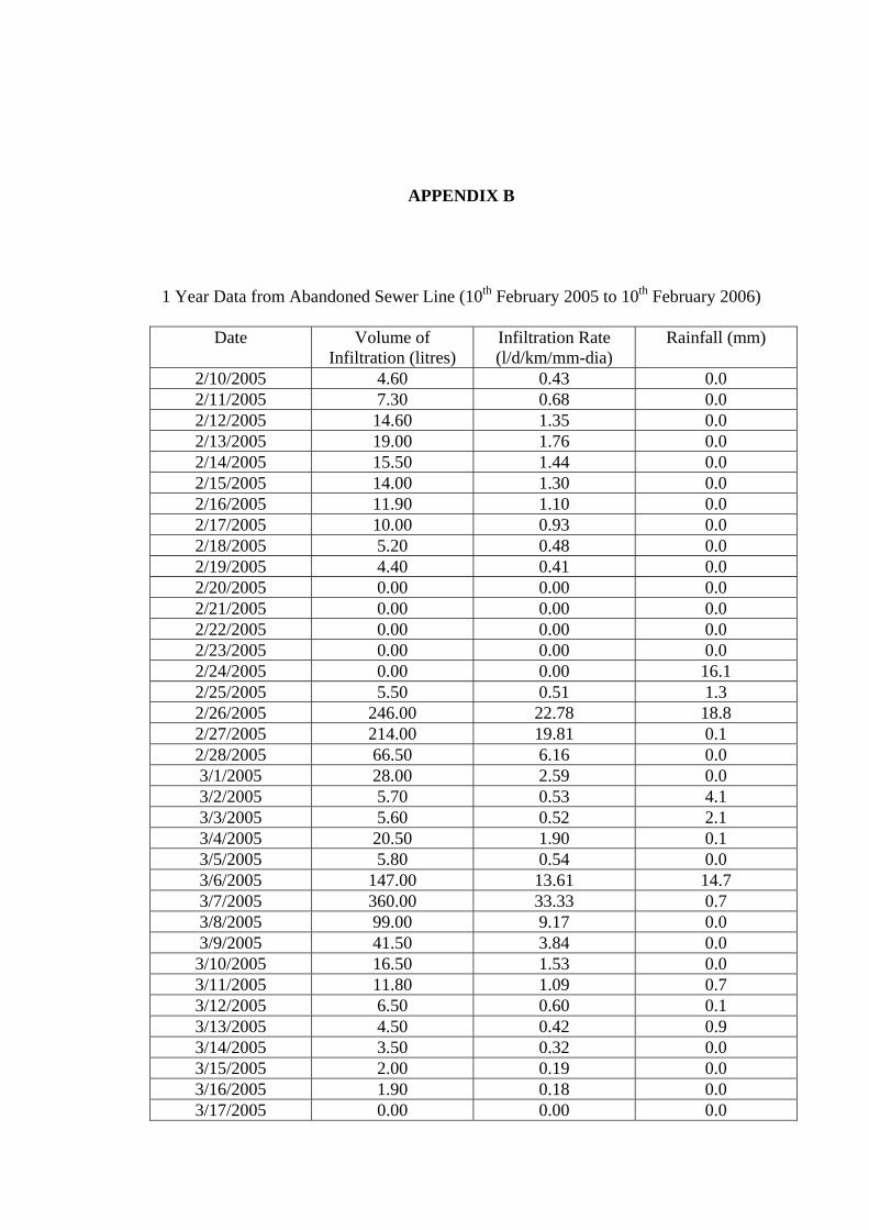
APPENDIX B
1 Year Data from Abandoned Sewer Line (10th February 2005 to 10th February 2006)
Date Volume of Infiltration (litres)
Infiltration Rate (l/d/km/mm-dia)
Rainfall (mm)
2/10/2005 4.60 0.43 0.0 2/11/2005 7.30 0.68 0.0 2/12/2005 14.60 1.35 0.0 2/13/2005 19.00 1.76 0.0 2/14/2005 15.50 1.44 0.0 2/15/2005 14.00 1.30 0.0 2/16/2005 11.90 1.10 0.0 2/17/2005 10.00 0.93 0.0 2/18/2005 5.20 0.48 0.0 2/19/2005 4.40 0.41 0.0 2/20/2005 0.00 0.00 0.0 2/21/2005 0.00 0.00 0.0 2/22/2005 0.00 0.00 0.0 2/23/2005 0.00 0.00 0.0 2/24/2005 0.00 0.00 16.1 2/25/2005 5.50 0.51 1.3 2/26/2005 246.00 22.78 18.8 2/27/2005 214.00 19.81 0.1 2/28/2005 66.50 6.16 0.0 3/1/2005 28.00 2.59 0.0 3/2/2005 5.70 0.53 4.1 3/3/2005 5.60 0.52 2.1 3/4/2005 20.50 1.90 0.1 3/5/2005 5.80 0.54 0.0 3/6/2005 147.00 13.61 14.7 3/7/2005 360.00 33.33 0.7 3/8/2005 99.00 9.17 0.0 3/9/2005 41.50 3.84 0.0 3/10/2005 16.50 1.53 0.0 3/11/2005 11.80 1.09 0.7 3/12/2005 6.50 0.60 0.1 3/13/2005 4.50 0.42 0.9 3/14/2005 3.50 0.32 0.0 3/15/2005 2.00 0.19 0.0 3/16/2005 1.90 0.18 0.0 3/17/2005 0.00 0.00 0.0
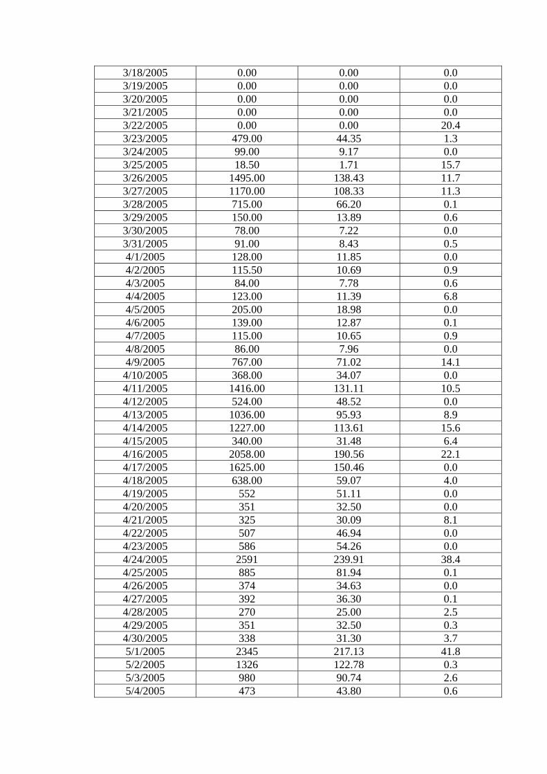
3/18/2005 0.00 0.00 0.0 3/19/2005 0.00 0.00 0.0 3/20/2005 0.00 0.00 0.0 3/21/2005 0.00 0.00 0.0 3/22/2005 0.00 0.00 20.4 3/23/2005 479.00 44.35 1.3 3/24/2005 99.00 9.17 0.0 3/25/2005 18.50 1.71 15.7 3/26/2005 1495.00 138.43 11.7 3/27/2005 1170.00 108.33 11.3 3/28/2005 715.00 66.20 0.1 3/29/2005 150.00 13.89 0.6 3/30/2005 78.00 7.22 0.0 3/31/2005 91.00 8.43 0.5 4/1/2005 128.00 11.85 0.0 4/2/2005 115.50 10.69 0.9 4/3/2005 84.00 7.78 0.6 4/4/2005 123.00 11.39 6.8 4/5/2005 205.00 18.98 0.0 4/6/2005 139.00 12.87 0.1 4/7/2005 115.00 10.65 0.9 4/8/2005 86.00 7.96 0.0 4/9/2005 767.00 71.02 14.1 4/10/2005 368.00 34.07 0.0 4/11/2005 1416.00 131.11 10.5 4/12/2005 524.00 48.52 0.0 4/13/2005 1036.00 95.93 8.9 4/14/2005 1227.00 113.61 15.6 4/15/2005 340.00 31.48 6.4 4/16/2005 2058.00 190.56 22.1 4/17/2005 1625.00 150.46 0.0 4/18/2005 638.00 59.07 4.0 4/19/2005 552 51.11 0.0 4/20/2005 351 32.50 0.0 4/21/2005 325 30.09 8.1 4/22/2005 507 46.94 0.0 4/23/2005 586 54.26 0.0 4/24/2005 2591 239.91 38.4 4/25/2005 885 81.94 0.1 4/26/2005 374 34.63 0.0 4/27/2005 392 36.30 0.1 4/28/2005 270 25.00 2.5 4/29/2005 351 32.50 0.3 4/30/2005 338 31.30 3.7 5/1/2005 2345 217.13 41.8 5/2/2005 1326 122.78 0.3 5/3/2005 980 90.74 2.6 5/4/2005 473 43.80 0.6
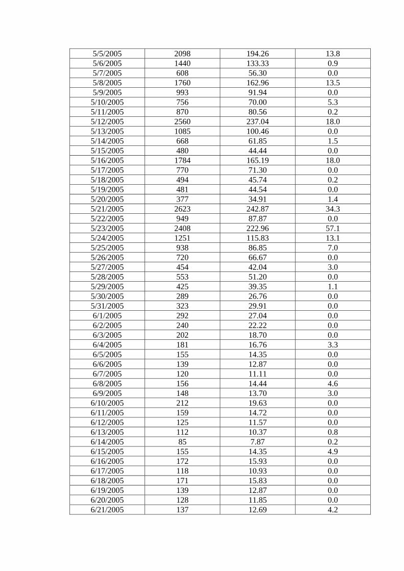
5/5/2005 2098 194.26 13.8 5/6/2005 1440 133.33 0.9 5/7/2005 608 56.30 0.0 5/8/2005 1760 162.96 13.5 5/9/2005 993 91.94 0.0 5/10/2005 756 70.00 5.3 5/11/2005 870 80.56 0.2 5/12/2005 2560 237.04 18.0 5/13/2005 1085 100.46 0.0 5/14/2005 668 61.85 1.5 5/15/2005 480 44.44 0.0 5/16/2005 1784 165.19 18.0 5/17/2005 770 71.30 0.0 5/18/2005 494 45.74 0.2 5/19/2005 481 44.54 0.0 5/20/2005 377 34.91 1.4 5/21/2005 2623 242.87 34.3 5/22/2005 949 87.87 0.0 5/23/2005 2408 222.96 57.1 5/24/2005 1251 115.83 13.1 5/25/2005 938 86.85 7.0 5/26/2005 720 66.67 0.0 5/27/2005 454 42.04 3.0 5/28/2005 553 51.20 0.0 5/29/2005 425 39.35 1.1 5/30/2005 289 26.76 0.0 5/31/2005 323 29.91 0.0 6/1/2005 292 27.04 0.0 6/2/2005 240 22.22 0.0 6/3/2005 202 18.70 0.0 6/4/2005 181 16.76 3.3 6/5/2005 155 14.35 0.0 6/6/2005 139 12.87 0.0 6/7/2005 120 11.11 0.0 6/8/2005 156 14.44 4.6 6/9/2005 148 13.70 3.0 6/10/2005 212 19.63 0.0 6/11/2005 159 14.72 0.0 6/12/2005 125 11.57 0.0 6/13/2005 112 10.37 0.8 6/14/2005 85 7.87 0.2 6/15/2005 155 14.35 4.9 6/16/2005 172 15.93 0.0 6/17/2005 118 10.93 0.0 6/18/2005 171 15.83 0.0 6/19/2005 139 12.87 0.0 6/20/2005 128 11.85 0.0 6/21/2005 137 12.69 4.2
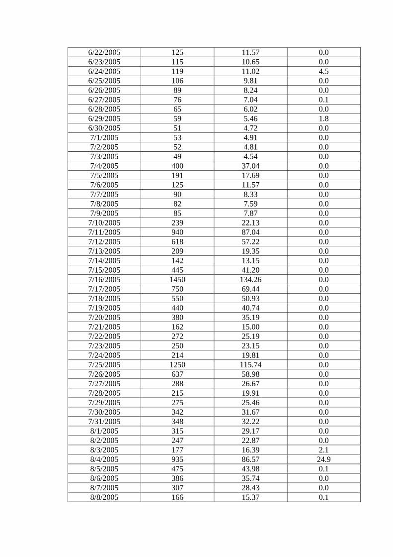
6/22/2005 125 11.57 0.0 6/23/2005 115 10.65 0.0 6/24/2005 119 11.02 4.5 6/25/2005 106 9.81 0.0 6/26/2005 89 8.24 0.0 6/27/2005 76 7.04 0.1 6/28/2005 65 6.02 0.0 6/29/2005 59 5.46 1.8 6/30/2005 51 4.72 0.0 7/1/2005 53 4.91 0.0 7/2/2005 52 4.81 0.0 7/3/2005 49 4.54 0.0 7/4/2005 400 37.04 0.0 7/5/2005 191 17.69 0.0 7/6/2005 125 11.57 0.0 7/7/2005 90 8.33 0.0 7/8/2005 82 7.59 0.0 7/9/2005 85 7.87 0.0 7/10/2005 239 22.13 0.0 7/11/2005 940 87.04 0.0 7/12/2005 618 57.22 0.0 7/13/2005 209 19.35 0.0 7/14/2005 142 13.15 0.0 7/15/2005 445 41.20 0.0 7/16/2005 1450 134.26 0.0 7/17/2005 750 69.44 0.0 7/18/2005 550 50.93 0.0 7/19/2005 440 40.74 0.0 7/20/2005 380 35.19 0.0 7/21/2005 162 15.00 0.0 7/22/2005 272 25.19 0.0 7/23/2005 250 23.15 0.0 7/24/2005 214 19.81 0.0 7/25/2005 1250 115.74 0.0 7/26/2005 637 58.98 0.0 7/27/2005 288 26.67 0.0 7/28/2005 215 19.91 0.0 7/29/2005 275 25.46 0.0 7/30/2005 342 31.67 0.0 7/31/2005 348 32.22 0.0 8/1/2005 315 29.17 0.0 8/2/2005 247 22.87 0.0 8/3/2005 177 16.39 2.1 8/4/2005 935 86.57 24.9 8/5/2005 475 43.98 0.1 8/6/2005 386 35.74 0.0 8/7/2005 307 28.43 0.0 8/8/2005 166 15.37 0.1
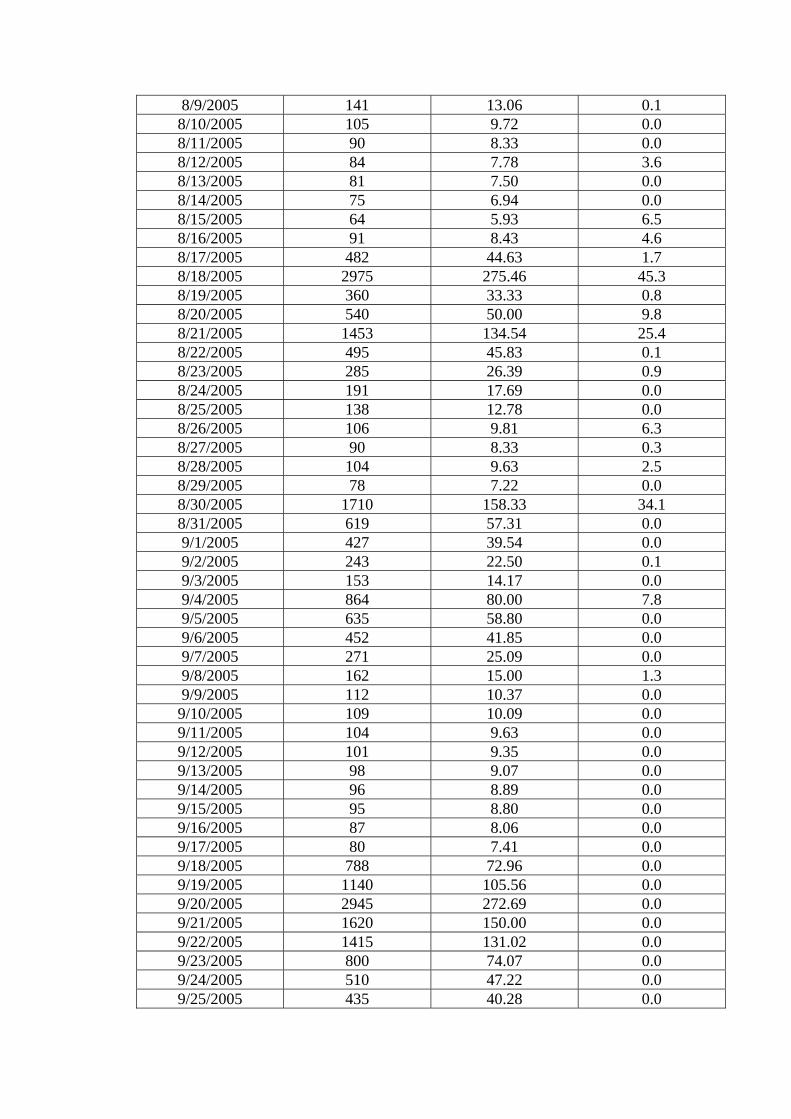
8/9/2005 141 13.06 0.1 8/10/2005 105 9.72 0.0 8/11/2005 90 8.33 0.0 8/12/2005 84 7.78 3.6 8/13/2005 81 7.50 0.0 8/14/2005 75 6.94 0.0 8/15/2005 64 5.93 6.5 8/16/2005 91 8.43 4.6 8/17/2005 482 44.63 1.7 8/18/2005 2975 275.46 45.3 8/19/2005 360 33.33 0.8 8/20/2005 540 50.00 9.8 8/21/2005 1453 134.54 25.4 8/22/2005 495 45.83 0.1 8/23/2005 285 26.39 0.9 8/24/2005 191 17.69 0.0 8/25/2005 138 12.78 0.0 8/26/2005 106 9.81 6.3 8/27/2005 90 8.33 0.3 8/28/2005 104 9.63 2.5 8/29/2005 78 7.22 0.0 8/30/2005 1710 158.33 34.1 8/31/2005 619 57.31 0.0 9/1/2005 427 39.54 0.0 9/2/2005 243 22.50 0.1 9/3/2005 153 14.17 0.0 9/4/2005 864 80.00 7.8 9/5/2005 635 58.80 0.0 9/6/2005 452 41.85 0.0 9/7/2005 271 25.09 0.0 9/8/2005 162 15.00 1.3 9/9/2005 112 10.37 0.0 9/10/2005 109 10.09 0.0 9/11/2005 104 9.63 0.0 9/12/2005 101 9.35 0.0 9/13/2005 98 9.07 0.0 9/14/2005 96 8.89 0.0 9/15/2005 95 8.80 0.0 9/16/2005 87 8.06 0.0 9/17/2005 80 7.41 0.0 9/18/2005 788 72.96 0.0 9/19/2005 1140 105.56 0.0 9/20/2005 2945 272.69 0.0 9/21/2005 1620 150.00 0.0 9/22/2005 1415 131.02 0.0 9/23/2005 800 74.07 0.0 9/24/2005 510 47.22 0.0 9/25/2005 435 40.28 0.0
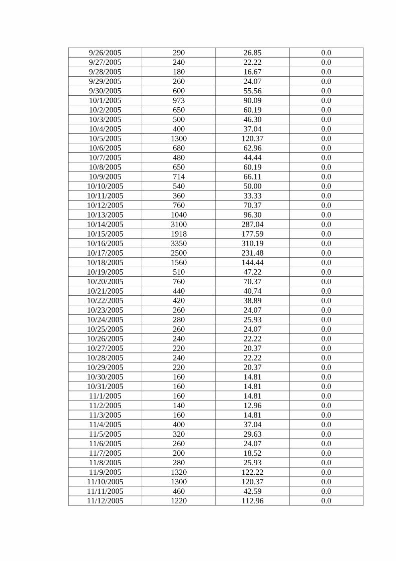
9/26/2005 290 26.85 0.0 9/27/2005 240 22.22 0.0 9/28/2005 180 16.67 0.0 9/29/2005 260 24.07 0.0 9/30/2005 600 55.56 0.0 10/1/2005 973 90.09 0.0 10/2/2005 650 60.19 0.0 10/3/2005 500 46.30 0.0 10/4/2005 400 37.04 0.0 10/5/2005 1300 120.37 0.0 10/6/2005 680 62.96 0.0 10/7/2005 480 44.44 0.0 10/8/2005 650 60.19 0.0 10/9/2005 714 66.11 0.0 10/10/2005 540 50.00 0.0 10/11/2005 360 33.33 0.0 10/12/2005 760 70.37 0.0 10/13/2005 1040 96.30 0.0 10/14/2005 3100 287.04 0.0 10/15/2005 1918 177.59 0.0 10/16/2005 3350 310.19 0.0 10/17/2005 2500 231.48 0.0 10/18/2005 1560 144.44 0.0 10/19/2005 510 47.22 0.0 10/20/2005 760 70.37 0.0 10/21/2005 440 40.74 0.0 10/22/2005 420 38.89 0.0 10/23/2005 260 24.07 0.0 10/24/2005 280 25.93 0.0 10/25/2005 260 24.07 0.0 10/26/2005 240 22.22 0.0 10/27/2005 220 20.37 0.0 10/28/2005 240 22.22 0.0 10/29/2005 220 20.37 0.0 10/30/2005 160 14.81 0.0 10/31/2005 160 14.81 0.0 11/1/2005 160 14.81 0.0 11/2/2005 140 12.96 0.0 11/3/2005 160 14.81 0.0 11/4/2005 400 37.04 0.0 11/5/2005 320 29.63 0.0 11/6/2005 260 24.07 0.0 11/7/2005 200 18.52 0.0 11/8/2005 280 25.93 0.0 11/9/2005 1320 122.22 0.0 11/10/2005 1300 120.37 0.0 11/11/2005 460 42.59 0.0 11/12/2005 1220 112.96 0.0
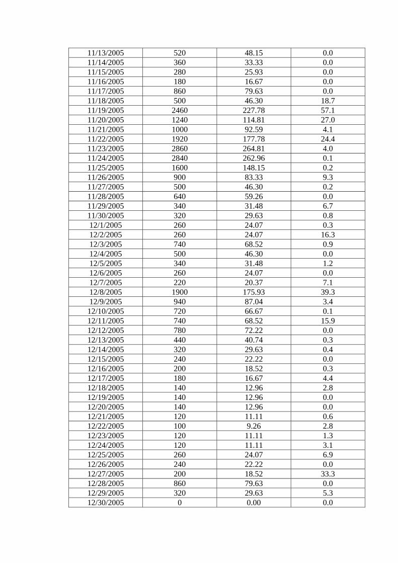
11/13/2005 520 48.15 0.0 11/14/2005 360 33.33 0.0 11/15/2005 280 25.93 0.0 11/16/2005 180 16.67 0.0 11/17/2005 860 79.63 0.0 11/18/2005 500 46.30 18.7 11/19/2005 2460 227.78 57.1 11/20/2005 1240 114.81 27.0 11/21/2005 1000 92.59 4.1 11/22/2005 1920 177.78 24.4 11/23/2005 2860 264.81 4.0 11/24/2005 2840 262.96 0.1 11/25/2005 1600 148.15 0.2 11/26/2005 900 83.33 9.3 11/27/2005 500 46.30 0.2 11/28/2005 640 59.26 0.0 11/29/2005 340 31.48 6.7 11/30/2005 320 29.63 0.8 12/1/2005 260 24.07 0.3 12/2/2005 260 24.07 16.3 12/3/2005 740 68.52 0.9 12/4/2005 500 46.30 0.0 12/5/2005 340 31.48 1.2 12/6/2005 260 24.07 0.0 12/7/2005 220 20.37 7.1 12/8/2005 1900 175.93 39.3 12/9/2005 940 87.04 3.4 12/10/2005 720 66.67 0.1 12/11/2005 740 68.52 15.9 12/12/2005 780 72.22 0.0 12/13/2005 440 40.74 0.3 12/14/2005 320 29.63 0.4 12/15/2005 240 22.22 0.0 12/16/2005 200 18.52 0.3 12/17/2005 180 16.67 4.4 12/18/2005 140 12.96 2.8 12/19/2005 140 12.96 0.0 12/20/2005 140 12.96 0.0 12/21/2005 120 11.11 0.6 12/22/2005 100 9.26 2.8 12/23/2005 120 11.11 1.3 12/24/2005 120 11.11 3.1 12/25/2005 260 24.07 6.9 12/26/2005 240 22.22 0.0 12/27/2005 200 18.52 33.3 12/28/2005 860 79.63 0.0 12/29/2005 320 29.63 5.3 12/30/2005 0 0.00 0.0
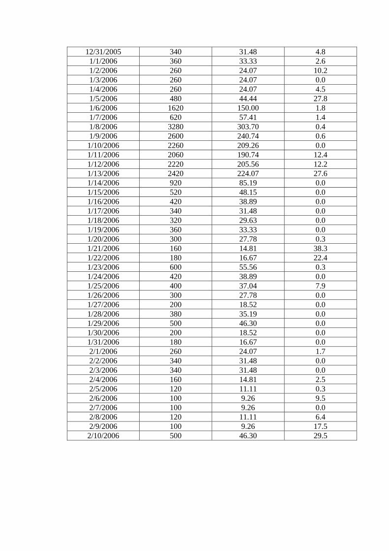
12/31/2005 340 31.48 4.8 1/1/2006 360 33.33 2.6 1/2/2006 260 24.07 10.2 1/3/2006 260 24.07 0.0 1/4/2006 260 24.07 4.5 1/5/2006 480 44.44 27.8 1/6/2006 1620 150.00 1.8 1/7/2006 620 57.41 1.4 1/8/2006 3280 303.70 0.4 1/9/2006 2600 240.74 0.6 1/10/2006 2260 209.26 0.0 1/11/2006 2060 190.74 12.4 1/12/2006 2220 205.56 12.2 1/13/2006 2420 224.07 27.6 1/14/2006 920 85.19 0.0 1/15/2006 520 48.15 0.0 1/16/2006 420 38.89 0.0 1/17/2006 340 31.48 0.0 1/18/2006 320 29.63 0.0 1/19/2006 360 33.33 0.0 1/20/2006 300 27.78 0.3 1/21/2006 160 14.81 38.3 1/22/2006 180 16.67 22.4 1/23/2006 600 55.56 0.3 1/24/2006 420 38.89 0.0 1/25/2006 400 37.04 7.9 1/26/2006 300 27.78 0.0 1/27/2006 200 18.52 0.0 1/28/2006 380 35.19 0.0 1/29/2006 500 46.30 0.0 1/30/2006 200 18.52 0.0 1/31/2006 180 16.67 0.0 2/1/2006 260 24.07 1.7 2/2/2006 340 31.48 0.0 2/3/2006 340 31.48 0.0 2/4/2006 160 14.81 2.5 2/5/2006 120 11.11 0.3 2/6/2006 100 9.26 9.5 2/7/2006 100 9.26 0.0 2/8/2006 120 11.11 6.4 2/9/2006 100 9.26 17.5 2/10/2006 500 46.30 29.5