Embed Size (px)
Citation preview

Vol. 25, No. 2, December 2018
IN THIS ISSUE:
� e case for convergence: assessing regional income distribution in Asia and the Paci� c
Arun Frey
Measuring autonomy: evidence from Bangladesh
Ana Vaz, Sabina Alkire, Agnes Quisumbing and Esha Sraboni
Factors in� uencing maternal health care in Nepal: the role of socioeconomic interaction
Sharmistha Self and Richard Grabowski
Price co-movements, commonalities and responsiveness to monetary policy: empirical analysis under Indian conditions
Anuradha Patnaik
Measuring creative economy in Indonesia: issues and challenges in data collection
Eni Lestariningsih, Karmila Maharani and Titi Kanti Lestari
Vol. 25, N
o. 2, Decem
ber 2018

The shaded areas of the map indicate ESCAP members and associate members.*
The Economic and Social Commission for Asia and the Pacific (ESCAP) serves as the United Nations’ regional hub, promoting cooperation among countries to achieve inclusive and sustainable development. As the largest regional intergovernmental platform with 53 member States and 9 associate members, ESCAP has emerged as a strong regional think-tank, offering countries sound analytical products that shed light on the evolving economic, social and environmental dynamics of the region. The Commission’s strategic focus is to deliver on the 2030 Agenda for Sustainable Development, which it does by reinforcing and deepening regional cooperation and integration in order to advance connectivity, financial cooperation and market integration. The research and analysis undertaken by ESCAP coupled with its policy advisory services, capacity building and technical assistance to governments aims to support countries’ sustainable and inclusive development ambitions.
*The designations employed and the presentation of material on this map do not imply the expression of any opinion whatsoever on the part of the Secretariat of the United Nations concerning the legal status of any country, territory, city or area or of its authorities, or concerning the delimitation of its frontiers or boundaries.

New York, 2019

ii
ASIA-PACIFICSUSTAINABLE DEVELOPMENT JOURNALVol. 25, No. 2, December 2018
United Nations publicationSales No. E.19.II.F.99Copyright © United Nations 2019All rights reservedPrinted in ThailandISBN: 978-92-1-120789-7e-ISBN: 978-92-1-004100-3ISSN (print): 2617-8400ISSN (online): 2617-8419ST/ESCAP/2855
Cover design: Nina Loncar
This publication may be reproduced in whole or in part for educational or non-profit purposes without special permission from the copyright holder, provided that the source is acknowledged. The ESCAP Publications Office would appreciate receiving a copy of any publication that uses this publication as a source.
No use may be made of this publication for resale or any other commercial purpose whatsoever without prior permission. Applications for such permission, with a statement of the purpose and extent of reproduction, should be addressed to the Secretary of the Publications Board, United Nations, New York.

iii
Editorial Advisory Board
Kaushik Basu Professor of Economics and C. Marks Professor of International Studies Department of Economics, Cornell University
Martin Ravallion Edmond D. Villani Professor of Economics Georgetown University
Sabina Alkire Director of the Oxford Poverty and Human Development Initiative (OPHI) Oxford Department of International Development, University of Oxford
Naila Kabeer Professor of Gender and Development, Department of Gender StudiesLondon School of Economics and Political Science
Li Xiaoyun Chief Senior Advisor at the International Poverty Reduction Centre in China, and Director of OECD/China-DAC Study Group, Chair of the Network of Southern Think Tanks (NeST) and Chair of China International Development Research
Network
Shigeo Katsu President, Nazarbayev University
Ehtisham Ahmad Visiting Senior Fellow Asia Research Centre, London School of Economics and Political Science
Myrna S. AustriaSchool of Economics, De La Salle University
Chief Editors
Patrik AnderssonActing Director, Social Development Division (SDD) of ESCAP
Hamza Ali MalikDirector, Macroeconomic Policy and Financing for Development Division (MPFD) of ESCAP
Editors
Ermina SokouChief, Sustainable Socioeconomic Transformation Section, SDD
Cai CaiChief, Gender Equality and Social Inclusion Section, SDD
Sabine HenningChief, Sustainable Demographic Transition Section, SDD
Oliver PaddisonChief, Countries with Special Needs Section, MPFD
Sweta SaxenaChief, Macroeconomic Policy and Analysis Section, MPFD
Tientip SubhanijChief, Financing for Development Section, MPFD
Editorial Assistants
Gabriela SpaizmannPannipa Jangvithaya
iv
EDITORIAL STATEMENT
The Asia-Pacific Sustainable Development Journal (APSDJ) is published twice a year by the Economic and Social Commission for Asia and the Pacific. It aims to stimulate and enrich research in the formulation of policy in the Asia-Pacific region towards the fulfillment of the 2030 Agenda for Sustainable Development.
APSDJ welcomes the submission of original contributions on themes and issues related to sustainable development that are policy-oriented and relevant to Asia and the Pacific. Articles should be centred on discussing challenges pertinent to one or more dimensions of sustainable development, policy options and implications and/or policy experiences that may be of benefit to the region.
Manuscripts should be sent to:
Chief Editors Asia-Pacific Sustainable Development Journal
Social Development Division and Macroeconomic Policy and Financing for Development Division United Nations Economic and Social Commission for Asia and the Pacific
United Nations Building, Rajadamnern Nok Avenue Bangkok 10200, Thailand Email: [email protected]
For more details, please visit www.unescap.org/apsdj.

v
The Editorial Board of the Asia-Pacific Sustainable Development Journal wishes to express its gratitude and appreciation to all of their reviewers for their invaluable contributions to the 2018 issues of the Journal.
Feriansyah Abdullah Vasantha Kandiah
Anthony Abeykoon Vinish Kathuria
Aradhna Aggarwal Nguyen Viet Khoi
Salman Asim Jonathon Khoo
N. R. Bhanumurthy Philippe Lebailly
Sai Sailaja Bharatam Aswini Kumar Mishra
Alain Brousseau Sangita Misra
Hukum Chandra Aadil Nakhoda
Francesca de Nicola Arman Bidarbakht Nia
Pierangelo De Pace Isabel Medalho Pereira Rodrigues
Filipe Lage de Sousa Janak Raj
Rebecca Siu Wai Fun Niranjan Sarangi
Bhakta Gubhaju Predrag Savic
Hyejoon Im Kunal Sen
Shireen Jejeebhoy Kyoko Shimamoto
Joosung Jun Miranda Stewart
Azizkhan Khankhodjaev Afsaneh Yazdani

vi

vii
ASIA-PACIFIC SUSTAINABLE DEVELOPMENT JOURNAL
Vol. 25, No. 2, December 2018
CONTENTS
Page
Arun Frey The case for convergence: assessing regional income distribution in Asia and the Pacific
1
Ana Vaz, Sabina Alkire, Agnes Quisumbing and Esha Sraboni
Measuring autonomy: evidence from Bangladesh
21
Sharmistha Self and Richard Grabowski
Factors influencing maternal health care in Nepal: the role of socioeconomic interaction
53
Anuradha Patnaik Price co-movements, commonalities and responsiveness to monetary policy: empirical analysis under Indian conditions
77
Eni Lestariningsih, Karmila Maharani andTiti Kanti Lestari
Measuring creative economy in Indonesia: issues and challenges in data collection
99

Explanatory notes
References to dollars ($) are to United States dollars, unless otherwise stated.
References to “tons” are to metric tons, unless otherwise specified.
A solidus (/) between dates (e.g. 1980/81) indicates a financial year, a crop year or an academic year.
Use of a hyphen between dates (e.g. 1980-1985) indicates the full period involved, including the
beginning and end years.
The following symbols have been used in the tables throughout the journal:
Two dots (..) indicate that data are not available or are not separately reported.
An em-dash (—) indicates that the amount is nil or negligible.
A hyphen (-) indicates that the item is not applicable.
A point (.) is used to indicate decimals.
A space is used to distinguish thousands and millions.
Totals may not add precisely because of rounding.
The designations employed and the presentation of the material in this publication do not imply
the expression of any opinion whatsoever on the part of the Secretariat of the United Nations
concerning the legal status of any country, territory, city or area or of its authorities, or concerning
the delimitation of its frontiers or boundaries.
Where the designation “country or area” appears, it covers countries, territories, cities or areas.
Bibliographical and other references have, wherever possible, been verified. The United Nations
bears no responsibility for the availability or functioning of URLs belonging to outside entities.
The opinions, figures and estimates set forth in this publication are the responsibility of the authors
and should not necessarily be considered as reflecting the views or carrying the endorsement of the
United Nations. Mention of firm names and commercial products does not imply the endorsement
of the United Nations.

1
THE CASE FOR CONVERGENCE: ASSESSING REGIONAL INCOME DISTRIBUTION
IN ASIA AND THE PACIFIC
Arun Frey*
This paper considers income inequality in Asia and the Pacific, examining whether there has been an increase or decrease in income inequality among countries in the region in recent decades. By analysing the position of countries’ GDP per capita relative to that of a reference economy (Australia), the study finds that between the years 1970 and 2014, most of the region’s less affluent countries were able to catch up in relative terms, allowing them to slowly move up the income matrix towards higher tier groups. Subregional examination reveals that most of the income convergence in the Asia-Pacific region was due to exceptional economic growth in East and North-East Asia and, to a lesser extent, in South-East Asia. While the paper shows that relative income differences between countries in the region have fallen since the 1970s, it points to the need for differentiating between relative and absolute measures of inequality. Insufficient convergence and substantial initial differences in GDP per capita have meant that, despite a decline in relative inequality, absolute differences in average income have grown during the same period.
JEL classification: E10, O40
Keywords: Asia and the Pacific, economic growth, between-country income inequality
* PhD Candidate, Department of Sociology, University of Oxford (email: [email protected]).
Much of the initial research of this paper was conducted at the United Nations Economic and Social Commission for Asia and the Pacific (ESCAP) in the Social Development Division. I would especially like to thank Patrik Andersson for early discussions that formed the framework underlying this analysis. The paper also benefited greatly from comments and discussions with Ermina Sokou.

Asia-Pacific Sustainable Development Journal Vol. 25, No. 2
2
I. INTRODUCTION
The Asia-Pacific region has experienced unprecedented economic growth over the past few decades. Regional gross domestic product (GDP) per capita more than doubled between 1990 and 2014, while global GDP per capita grew by 50 per cent. This surge in economic growth enabled increased investment in human capital and created job opportunities throughout the region, lifting millions of people out of extreme poverty and improving overall well-being. Since 1990, the poverty headcount in the region has decreased sharply, from 30 per cent to some 10 per cent, pointing to impressive strides made in poverty alleviation (ESCAP, 2017).
Despite this sustained economic development and the substantial reductions in poverty, progress has disproportionately benefited the wealthiest members of society, increasing inequalities between the rich and poor in many parts of Asia and the Pacific. High inequality has not only stifled economic progress, but has also adversely affected feelings of trust and social cohesion (ESCAP, 2017; 2018). These rising levels of inequality within countries triggered public concern and academic interest, contributing to a stand-alone goal on inequality in the United Nations 2030 Agenda for Sustainable Development. Under Sustainable Development Goal 10 (SDG 10), reducing “inequalities within and among countries” is a core policy priority to ensure a sustainable and prosperous future for all. While much of the discourse surrounding inequality focuses on within-country dynamics, this paper considers the second component of SDG 10 – inequality among countries – and seeks to answer the question of how economic growth in Asia and the Pacific has affected regional income distribution.
To intuitively visualize changes in regional income dynamics over time, this study reports countries’ GDP per capita in relation to the GDP per capita of Australia. It finds that regional income inequality has fallen continuously since 1970 and converged from a twin peaked to a flatter shaped distribution. The reason is that poorer countries in the region have often grown at a faster pace than richer ones. However, upon closer inspection at the subregional level, one finds substantial differences in this process. While in almost all countries in Asia and the Pacific average annual growth rates between 1970 and 2014 were higher than in Australia (the reference economy), the rate of growth was generally strongest for countries from East and North-East Asia. By comparison, North and Central Asia experienced less growth in the initial years following the collapse of the Soviet Union, as economies were in transition and undergoing structural transformation.
Descriptive analysis further shows that, while relative between-country inequality fell in the region, absolute income differences grew in almost all cases. In other words, relative convergence in countries’ income was not sufficient to overcome the

The case for convergence assessing regional income distribution in Asia and the Pacific
3
significant initial gaps in GDP per capita between rich and poor countries, leading to a widening of the absolute income gap. Thus, despite impressive – and unparalleled – economic growth, substantial differences in absolute incomes between countries in Asia and the Pacific remain.
The implications of these findings are threefold: (1) the rate at which countries in Asia and the Pacific have developed in recent decades has reduced the relative income gap between rich and poor nations; (2) the reductions in poverty and relative income inequality in the region have been heavily driven by the extraordinary growth periods within a few countries; (3) the relative changes in GDP per capita have failed to reflect the continuingly extensive, and in most cases growing, absolute gap in incomes between rich and poor countries.
II. SETTING THE STAGE: WHY INEQUALITY BETWEEN COUNTRIES MATTERS
Under SDG 10, member States pledge to “reduce inequality within and among countries”. Both components are captured within global inequality, which consists of inequality between countries (i.e. differences between countries’ average income) and inequality within countries (i.e. differences in individuals’ or households’ income within a country). In an increasingly globalized world, where factors of production are being moved to areas with lower costs, and inter-connected individuals are better able to compare living standards across borders, notions of “fairness” and “equality” are being stretched beyond territorial boundaries (Milanovic, 2012a; 2012b). The issue of inequality should therefore not only be seen as a national priority, but also understood at the regional and international level.
While much of the academic and political discourse has focused on within-country inequality, this paper explores the second component of SDG 10, analysing income differences between countries. Despite recent academic focus on inequality within nations, the largest contribution to global income inequality stems from differences between countries (Pinkovskiy and Sala-i-Martin, 2009). Milanovic (2005) finds that between 71 per cent to 83 per cent of global inequality is the result of differences in countries’ GDP per capita.1 Thus, GDP per capita growth is a vital instrument in altering global income dynamics. Accordingly, this paper sets out to descriptively explore changes in regional income distribution within Asia and the Pacific between 1970 and 2014.
1 This depends on whether the Palma ratio or the Gini coefficient is used as a measure of inequality. Note that Milanovic also treats rural and urban regions in China and India as separate in his analysis, which may have an influence on his estimates.
Asia-Pacific Sustainable Development Journal Vol. 25, No. 2
4
During the 19th century and into the first half of the 20th century, income inequality between countries increased across the world (Roser, 2019; Bourguignon and Morrison, 2002). It was initially argued that countries would continue to diverge (Pritchett, 1997) or polarize into two separate distributions, one rich and one poor (Quah, 1993; 1996). However, evidence showed that countries’ incomes began to converge in the 1970s, with the trend accelerating in recent years (Kane, 2016). According to Hellebrandt and Mauro (2015), this resulted in a decline in global inequality, with the Gini coefficient dropping from 68.4 to 64.9 between 2003 and 2013. However, Milanovic and Lakner (2015) cautioned that the underreporting of high incomes may have biased this observed decline in global inequality. Changes in the global distribution of income also appeared to have been driven by China and India, the world’s most populous countries. Accordingly, some have argued that the fall in global inequality was largely due to China’s and India’s growth, which overshadowed stagnant development in smaller island States and less populous countries (Bourguignon, 2011; DESA, 2015). To enable a better examination of regional income dynamics, this paper restricts its analysis to Asia and the Pacific, exploring whether countries’ incomes in this region have converged or diverged since 1970.
III. DATA
In accordance with previous studies, data for this study was retrieved from the Penn World Table database (Feenstra, Inklaar and Timmer, 2015). As is the case with Penn World Table data, economic variables are denominated in a common currency, which allows for precise comparisons of countries’ gross domestic product over time. Unfortunately, Penn World Table data on the Asia-Pacific region is limited. The United Nations Economic and Social Commission for Asia and the Pacific (ESCAP) lists 53 members and 9 associate members, of which 58 are located within Asia and the Pacific.2 Data for the period of 1970 to 2014 was available for only 28 of the 58 countries located within the region. However, a number of these countries did not exist prior to 1990. If this start date is used instead, it is possible to expand the dataset to include Armenia, Azerbaijan, Georgia, Kazakhstan, Kyrgyzstan, the Russian Federation, Tajikistan, Turkmenistan and Uzbekistan (members of the former Soviet Union), resulting in a total sample of 37 countries across 24 years. Taken together, this broader sample includes data for all Asian countries (except Afghanistan, the Democratic People’s Republic of Korea and Timor-Leste), but provides for only limited observations in the Pacific region. Thus, although it may not be possible to make generalizations for Pacific countries, the research does accurately depict income dynamics within Asia. To balance breadth of countries with number of years, analyses
2 France, the Netherlands, the United Kingdom of Great Britain and Northern Island and the United States of America are ESCAP members, but are located outside of the Asia-Pacific region.
The case for convergence assessing regional income distribution in Asia and the Pacific
5
have been conducted on both the limited sample reaching back to 1970 as well as the broader sample starting in 1990.3
For each available country, the real GDP per capita4 was used to measure mean income. While there are drawbacks and advantages to using national accounts data over household data, this paper chose to rely on GDP per capita figures due to data availability.5 The Penn World Table figures have been adjusted for purchasing power parity (PPP) and reported in 2011 United States dollars to enable accurate cross-country comparisons over time.
Countries are used as the primary unit of analysis in order to avoid a skewing of results in favour of large countries. The Asia-Pacific region is home to countries with both very large and very small populations. China, India and Indonesia account for two-thirds of the region’s total population. Bhutan, by comparison, is home to less than 0.02 per cent of the population in Asia and the Pacific. Population-weighted estimates would thus likely skew results in favour of population-rich countries at the expense of small member States.
IV. METHODS
This paper sets out to present a descriptive and intuitive account of changes in relative income in Asia and the Pacific between 1970 and 2014. In order to do this, countries’ GDP per capita is reported in relation to the GDP of Australia, and categorized into six income tiers, following Jones’ (1997) income intervals (see table 1). As a developed country with one of the highest GDP per capita rates within the region, Australia was selected as the benchmark category, in order to capture whether countries in the Asia-Pacific region had grown closer together or further apart within recent years. Australia was favoured over other countries with higher GDP per capita due to its stable growth rate (see appendix, figure A).6 By reporting countries’ income as a percentage of Australia’s, it was possible to compare their relative income at different points in time, and thus visualize where and when convergence may have taken place. Table 1 outlines the different income tier classifications: Tier 6 reflects the poorest countries with a GDP per capita of less than or equal to 5 per cent of that of Australia; Tier 5 reflects countries between 5 and 10 per cent, and so forth (see table 1).
3 See appendix, table A for a full breakdown of data availability by ESCAP member States.4 Expenditure-side real GDP at chained PPPs (in 2011 United States dollars).5 See Pinkovskiy and Sala-i-Martin (2009) and Milanovic (2005) for a discussion on the drawbacks
and advantages of using GDP per capita over household data. 6 Member States with a higher GDP per capita than that of Australia are Brunei Darussalam (1970,
1980, 1990, 2000, 2010, 2014), Hong Kong, China (2010, 1014), Japan (1990), Macao, China (2010, 2014), and Singapore (2000, 2010, 2014).

Asia-Pacific Sustainable Development Journal Vol. 25, No. 2
6
Table 1. Tier group classification cut-offs
Tier groups Cut-off points
Tier 1 0.80 < y
Tier 2 0.40 < y ≤ 0.80
Tier 3 0.20 < y ≤ 0.40
Tier 4 0.10 < y ≤ 0.20
Tier 5 0.05 < y ≤ 0.10
Tier 6 y ≤ 0.05
Source: Tier groups based on Jones (1997).
Note: “y” refers to a country’s income relative to that of the reference economy (Australia).
V. INCOME CONVERGENCE IN ASIA AND THE PACIFIC BETWEEN 1970 AND 2014
Figure 1 depicts the relative regional income distribution in the Asia-Pacific region for the years 1970, 1990, 2010 and 2014. In 1970, the distribution of income across the region was noticeably unequal. The region was divided into two segments: a larger segment of poor countries, with an average income of less than 25 per cent of Australia, and a smaller segment of countries with income levels comparable to that of Australia. Over the years, income distribution converged from a twin peak into a flat distribution. With each decade, the number of relative poor countries fell significantly, converging into a flatter-shaped income distribution by 2014.
Figure 1. Relative GDP per capita in Asia and the Pacific, 1970 to 2014
GDP per capita relative to Australia (percentage)
1970
1990
2010
2014
0.025
0.020
0.015
0.010
0.005
0
Den
sity
0 20 40 60 80 100

The case for convergence assessing regional income distribution in Asia and the Pacific
7
VI. FROM 1970 TO 1990: EAST ASIAN GROWTH MIRACLE, STAGNANT SOUTH ASIA
Although figure 1 shows that the regional GDP per capita distribution flattens over years, with poorer countries moving closer to richer ones, it does not provide any information on the scale of convergence for individual member States. To better illustrate this, countries’ relative position to Australia is visualized using Jones’ (1997) income tier groups.
Table 2 compares the position of 28 countries across income tier groups between 1970 and 1990. In 1970, the region was comprised of mostly poor countries. Twenty out of twenty-eight countries were listed in the bottom three income tiers. By 1990, this number had slightly decreased to 17 countries, while the number of high income countries (Tiers 1 and 2) had doubled from 4 to 8 countries. By 1990, 10 out of the 28 countries had moved towards higher tier categories, while 3 countries had fallen to a lower category and 15 countries had remained within their tier group. Although progress did occur in some countries, it tended to manifest itself at higher levels, such that, while the top income group grew, so did the bottom group, each adding two countries.
During this period, the group of countries known as “the Asian Tigers” made the biggest strides. The Republic of Korea was able to increase its average income from 11 per cent to 45 per cent by 1990, elevating the country from the tier group 4 to tier group 2. Similarly, both Hong Kong, China and Macao, China increased their position from tier group 3 to tier group 1. Indonesia, Mongolia, the Maldives (Tier 5 to Tier 4), Fiji, Malaysia (Tier 4 to Tier 3), Singapore (Tier 3 to Tier 2) and Japan (Tier 2 to 1) also experienced strong economic growth. In contrast, no country among the lowest tier group was able to sufficiently increase its relative income to move to a higher income tier group. Rather, India and Cambodia both experienced a decrease in relative income, moving down to the lowest tier.
Table 2. Income tier matrix between 1970 and 1990
1970
Tier 1 Tier 2 Tier 3 Tier 4 Tier 5 Tier 6
1990 Tier 1 2 1 2 58
Tier 2 1 1 1 3
Tier 3 1 2 3
Tier 4 4 3 7
17Tier 5 4 4
Tier 6 2 4 6
3 1 4 7 9 4 28
4 20

Asia-Pacific Sustainable Development Journal Vol. 25, No. 2
8
The matrix in table 2 reveals some convergence in countries’ income between 1970 and 1990. Out of the 13 countries that had moved income tiers, 10 shifted to higher income tier groups. However, the periods of growth differed considerably by subregion: most of the income convergence occurred in countries from East and North-East Asia and, to a lesser extent, from countries in South-East Asia. Poorer countries by contrast, especially those from South and South-West Asia, were not able to keep up with the East Asia growth spell, and only two countries moved income tiers groups – India sank from Tier 5 to Tier 6, and the Maldives rose from Tier 5 to Tier 4.
Radelet, Sachs and Lee (2001) identify the factors responsible for East Asia’s extraordinary economic growth between the 1970s and 1990s, and highlight what aspects enabled these economies to flourish while South Asian countries were left behind. First, economic policies were vital in determining growth performance: East Asia’s institutional quality and trade openness facilitated strong economic growth. South Asia, by contrast, practiced isolationist trade policies, enacting high tariffs that reduced international trade and negatively impacted GDP per capita growth rates. Second, a growing working-age population, combined with higher life expectancy and high levels of secondary education allowed countries in East and North-East Asia to capitalize on their growth potential relative to South Asia (Bloom and Williamson, 1997). Third, in addition to sound economic policies and favourable social and demographic conditions, “Asian Tiger” countries tended to be small, with very open economies which, despite relatively few resources, had a well-educated workforce – all factors that contributed significantly to their impressive growth. Conversely, the lower life expectancy in South Asian countries, coupled with a slower growth in the working-age population and a higher overall population growth, placed the subregion at a comparative disadvantage.
VII. 1990 TO 2014: ACCELERATING CONVERGENCE THROUGHOUT ASIA AND THE PACIFIC
Between 1990 and 2014 the region experienced much stronger income convergence. Nineteen out of twenty-eight countries moved to a higher income tier group, while only one, Fiji, fell to a lower tier. All other countries experienced significantly stronger growth rates than Australia during this period, allowing them to rise by one or two income tiers in the matrix (table 3). Remarkably, while there was no movement among the lowest group between 1970 and 1990, all six countries in the lowest income tier transitioned to higher income groups between 1990 and 2014. In fact, the majority of gains were made at lower levels, with India, Lao People’s Democratic Republic, Myanmar, Viet Nam (Tier 6 to Tier 4) and China (Tier 5 to Tier 3) each rising by two income tiers. At higher levels, Malaysia and Turkey rose from Tier 3 to Tier 2, and New Zealand, the Republic of Korea and Singapore joined the highest income group.

The case for convergence assessing regional income distribution in Asia and the Pacific
9
Table 3. Income tier matrix between 1990 and 2014
1990
Tier 1 Tier 2 Tier 3 Tier 4 Tier 5 Tier 6
2014 Tier 1 5 3 810
Tier 2 2 2
Tier 3 6 1 7
Tier 4 1 1 2 4 8
11Tier 5 1 2 3
Tier 6 0
5 3 3 7 4 6 28
8 17
Countries in South and South-West Asia fared poorly between 1970 and 1990, with only one country moving up to a higher income tier. However, this changed between 1990 and 2014, when eight out of the nine South and South-West Asian countries moved up to higher tier groups, catching up with the impressive growth performance of the economies in East and North-East Asia and South-East Asia. Improved economic policies and an increasing openness to the world market allowed many South and South-West Asian countries to capitalize on their growth potential, and slowly catch up to the growth rates of other countries in the region. Shifts in demographic dynamics also meant that the working-age population grew during this time, delivering a similar economic boost that had facilitated growth in East Asia two decades earlier. Meanwhile, the formerly fast-growing economies of Hong Kong, China, and the Republic of Korea were beginning to slow down, as their “catching up” phase concluded (Barro, 1991). A comparably stagnant economic growth period in Australia in recent years further added to this convergence process. As a result, the strong growth of countries in the lowest income category, combined with a slowing of growth at higher levels, has led to a decrease income inequality between countries in the Asia-Pacific region, with the level of convergence accelerating over the last two decades (Kane, 2016).
Comparing the relative income distribution in 2014 to that in 1970, there is not a single country that fell to a lower income tier. The rate of convergence is evidenced by the speed at which countries have moved towards higher income tiers over the 44-year span: 21 out of 28 countries moved to higher income tiers, of which more than half transitioned by two or more income tiers. This positive development points to the growth miracle that has taken place in many Asian countries. Since 1970, countries in the ESCAP region have benefitted from a range of social reforms, trade agreements, industrial development and sociodemographic shifts that have facilitated progressive growth and brought nations closer together, shrinking the income gap between rich and poor countries in the region.

Asia-Pacific Sustainable Development Journal Vol. 25, No. 2
10
Table 4. Income tier matrix between 1970 and 2014
1970
Tier 1 Tier 2 Tier 3 Tier 4 Tier 5 Tier 6
2014 Tier 1 3 1 3 1 810
Tier 2 1 1 2
Tier 3 3 4 7
Tier 4 2 3 3 8
11Tier 5 2 1 3
Tier 6 0
3 1 4 7 9 4 28
4 20
VIII. INCLUDING NORTH AND CENTRAL ASIA: INCOME CONVERGENCE, 1990-2014
A substantial number of ESCAP member States in North and Central Asia did not exist prior to the collapse of the Soviet Union. As a result, nine North and Central Asian countries – Armenia, Azerbaijan, Georgia, Russian Federation, Kazakhstan, Kyrgyzstan, Tajikistan, Turkmenistan and Uzbekista – were introduced into the analysis from 1990 to 2014, and are highlighted in bold in table 5.
Out of the nine countries, five of them – Kazakhstan, Russian Federation, Azerbaijan, Georgia and Uzbekistan – remained within their income tier. Only one country, Turkmenistan, managed to move up to a higher income tier group by 2014, migrating from Tier 3 to Tier 2, while doubling its GDP per capita. Three countries’ relative GDP per capita declined during the same period: Armenia’s average income declined slightly relative to Australia, with the country falling from Tier 3 to Tier 4; Kyrgyzstan and Tajikistan both suffered strong economic losses after 1990 with their relative income falling from 28 and 25 per cent to 8 and 6 per cent respectively, and dropping from Tier 3 to Tier 5 (table 5). Economies in North and Central Asia suffered severe economic shocks following the collapse of the Soviet Union, and generally performed worse than other countries in the region.

The case for convergence assessing regional income distribution in Asia and the Pacific
11
Table 5. Change in relative income tiers between 1990 and 2010, additional countries
1990
Tier 1 Tier 2 Tier 3 Tier 4 Tier 5 Tier 6
2014 Tier 1 5 3 813
Tier 2 2 2 + 1 5
Tier 3 2 6 1 9
Tier 4 1 + 1 1 + 1 2 4 10
15Tier 5 2 1 2 5
Tier 6 0
5 5 9 8 4 6 37
10 18
IX. DECLINES IN RELATIVE INEQUALITY, INCREASES IN ABSOLUTE INEQUALITY IN THE REGION
Despite reduced economic growth in North and Central Asia, regional income in Asia and the Pacific converged, with poorer countries’ average income generally growing at a greater rate than that of richer countries. While this can be seen as an improvement and a cause for celebration, it is important to acknowledge that this rests on a relative concept of income inequality. Individuals’ understanding of inequality, however, is not only based on relative differences, but is also tied to absolute gaps in earnings and incomes (Amiel and Cowell, 1992; 1999). To illustrate this point, consider the following: the doubling of two individuals’ income, from $10 to $20 for person A, and $100 to $200 for person B, respectively, would have no effect on relative income inequality between them – in both cases, person B earns ten times as much as person A. Yet, it is not unreasonable to assume that the second scenario (i.e. $20 and $200) may be perceived as far more unjust than the first, due to the large increase in the absolute income gap. The growing international debate about a rising income disparity between the rich and poor is a case in point (Niño-Zarazúa, Roope and Tarpe, 2017). Acknowledging these influences, many academics have called for a broadening of the debate on inequality beyond relative considerations (Ravaillon, 2003; Atkinson and Brandolini, 2010; Sreenivasan and Dhairiyarayar, 2013; Niño-Zarazúa, Roope and Tarpe, 2017).
To briefly visualize the ongoing disparity in absolute incomes between rich and poor countries, figure 2 plots changes in countries’ income gap relative to Australia between 1970 (1990 for North and Central Asia) and 2014. Income differences at the earliest year were indexed at zero to allow for better comparisons over time. Figures

Asia-Pacific Sustainable Development Journal Vol. 25, No. 2
12
below zero indicate that the difference between a country’s and Australia’s GDP per capita has increased between 2014 and 1970/1990, while a figure above zero means that there has been a reduction in absolute income differences.
As shown in figure 2, the absolute gap has increased in nearly all countries during the period under consideration. This may seem surprising at first, considering the convergence of relative regional income since 1970. However, large initial differences between Australia’s GDP per capita and that of most other countries in the region means that, despite its comparably slow growth, Australia’s GDP per capita nevertheless grew more in absolute terms than most countries in the region.
Figure 2. The absolute income gap to Australia has increased unfavourably for most countries in Asia and the Pacific, earliest year and 2014
Note: Country codes and names are as follows: ARM - Armenia, AZE - Azerbaijan, BGD - Bangladesh, BTN - Bhutan,
CHN - China, FJI - Fiji, GEO - Georgia, HGK - Hong Kong, China, IDN - Indonesia, IRN - Islamic Republic of Iran,
JPN - Japan, KAZ - Kazakhstan, KGZ - Kyrgyzstan, KOR - Republic of Korea, LKA - Sri Lanka, MDV - Maldives,
NZL - New Zealand, PAK - Pakistan, TKM - Turkmenistan.
Year1970/1990 2014
Paci�cSouth and South - West AsiaSouth - East AsiaEast and North - East AsiaNorth and Central Asia
JPN
KOR
HKG
KAZ
NZLTKM
AZE
MDVIRNCHNARM
IDN
LKAGEOBTNFJIKGZPAK
BGD
20 000
10 000
0
-10 000
-20 000
Di�
eren
ce to
Aus
tral
ia’s
GD
P pe
r cap
ita(U
nite
d St
ates
dol
lar,
inde
xed
to e
arlie
st y
ear)
The case for convergence assessing regional income distribution in Asia and the Pacific
13
Following Niño-Zarazúa, Roope and Tarpe (2017), this example illustrates the implications that different ways of reporting income inequalities can have on conversations surrounding this issue: in relative terms, income inequality between countries in Asia and the Pacific has reduced since the 1970s. However, insufficient relative convergence, together with high initial differences in GDP per capita between rich and poor countries have meant that, despite a reduction in relative inequality, absolute differences have increased throughout this period. China, the Asian-Pacific “economic miracle par excellence”, experienced an extraordinarily impressive annual GDP growth rate of 6.1 per cent in 2016 (World Bank, 2016). However, despite this exceptional performance, it would take China an additional 36 years of maintaining this growth rate to catch up to the GDP per capita level of Australia in 2016. These absolute gaps need to be taken into account when writing about changes in inequality dynamics, even if the focus is on a shift in relative terms. Clearly, societal understanding of what constitutes “fair” and “unfair” income distributions will also rest on absolute differences.
X. CONCLUSION
This paper has examined the extent to which income inequality among countries in Asia and the Pacific has converged since the 1970s. By analysing countries’ GDP per capita relative to that of Australia, the paper reveals that, over the past four and a half decades, the region has indeed been growing closer together. While Asia and the Pacific includes a variety of countries whose GDP per capita have grown remarkably during the period studied, this paper has also shown that other countries with less impressive growth records have consistently managed to catch up to the leading economy.
The analysis has also highlighted substantial shifts in subregional dynamics. Countries that were high performing in the 1970s, such as Japan, the Republic of Korea, or Hong Kong, China, have seen their growth rates stabilize, after having completed a “catching up” convergence process (Barro, 1991; Barro and Lee, 1994; Stokey, 2014). Moreover, while East and North-East Asian and South-East Asian economies grew rapidly between 1970 and 1990 due to favourable socioeconomic and demographic dynamics, South and South-West Asian countries have only recently capitalized on their growth potential and, as such, are arguably in the process of catching up to the growth miracle in other countries. Despite the setback of some North and Central Asian economies, current patterns suggest considerable convergence in relative incomes in Asia and the Pacific since 1970.
In attempting to answer the second component of SDG 10, the study finds that, on a regional level, relative inequality among countries has fallen. Thus, the idea of a diverging “twin peaks” phenomenon (Quah 1993; 1996), in which world income

Asia-Pacific Sustainable Development Journal Vol. 25, No. 2
14
distribution increasingly diverges into rich and poor country groups, has not held true within the Asian-Pacific context. Rather, relative inequality has been declining, with poorer countries catching up to the income levels of richer countries.
Relative considerations of income inequality, however, neglect the large, and often growing, absolute gaps between countries’ GDP per capita. While relative inequality fell during the study period, the absolute gap, in relation to Australia, increased in almost all countries at the same time. This means that, notwithstanding the comparably slower growth in Australia’s GDP per capita, and the faster economic growth in poorer countries’, the absolute income disparity continued to widen. Effects of inequality, especially those related to social cohesion, trust, unrest and instability, rest heavily on subjective feelings of injustice, which are in part tied to absolute differences in income. These absolute differences need to be reflected in research on income inequality.
Before concluding this paper, it is important to note its limitations. First, this is a descriptive account of income dynamics in Asia and the Pacific between 1970 and 2014, and therefore makes no claim to the mechanisms underlying this convergence process. Second, the extent and nature of convergence observed are naturally conditional on the benchmark economy. The reasons for selecting Australian GDP per capita as opposed to that of another economy are, as outlined above, due to it having one of the highest average incomes in the region throughout the period of analysis, combined with a stable annual growth rate. Lastly, this paper reveals nothing about within-country inequality. With many countries in the Asia-Pacific region experiencing an increase in income inequalities within their national borders (ESCAP, 2017), it is increasingly important to separate changes in regional income distribution into between-country and within-country dynamics. Bourguignon (2011) decomposes global inequality into between and within-country inequality, claiming that
it is remarkable that, despite rising within-country inequality, global inequality is decreasing at a fast pace. The problem, however, is that what is happening at the national level may be more important from a political economy perspective than what is happening at the global level. An increase in inequality at the national level may become a real obstacle to global inclusion and global development even though global inequality is decreasing (Bourguignon, 2011, p.13).
This paper sets the stage for future policy discussions on inequality from multiple vantage points. In relative terms, regional inequality has decreased, while in absolute terms it has increased. At the same time, within-country dynamics suggest that those countries experiencing the largest increases in mean income have also experienced the largest increase in inequality within their national borders.

The case for convergence assessing regional income distribution in Asia and the Pacific
15
REFERENCES
Amiel, Yoram, and Frank Cowell (1992). Measurement of income inequality: experimental test by questionnaire. Journal of Public Economics, vol. 47, No. 1, pp. 3-26.
______ (1999). Thinking about Inequality. Cambridge, MA: Cambridge University Press.
Atkinson, Anthony B., and Andrew Brandolini (2010). On analysing the world distribution of income. World Bank Economic Review, vol. 24, No. 1, pp. 1-37.
Barro, Robert J. (1991). Economic growth in a cross section of countries. The Quarterly Journal of Economics, vol. 106, No. 2, pp. 407-443.
Barro, Robert J., and Jong-Wha Lee (1994). Sources of economic growth. Carnegie-Rochester Conference Series on Public Policy, vol. 40, No.1, pp. 1-46.
Bloom, David E., and Jeffrey G. Williamson (1997). Demographic transitions and economic miracles in emerging Asia. World Bank Economic Review, vol. 12, No. 3, pp. 419-455.
Bourguignon, F. (2011). A Turning Point in Global Inequality… And Beyond? Washington, D.C.: World Bank. Available from http://siteresources.worldbank.org/EXTABCDE/Resources/7455676-1292528456380/7626791-1303141641402/7878676-1306270833789/Parallel-Session-6-Francois_Bourguignon.pdf.
Bourguignon, F., and C. Morrison (2002). Inequality among world citizens, 1820–1992. American Economic Review, vol. 92, No. 4, pp. 727-974.
Feenstra, Robert C., Robert Inklaar, and Marcel P. Timmer (2015). The next generation of the Penn World Table. American Economic Review, vol. 105, No. 10, pp. 3150-3182. Available from www.ggdc.net/pwt.
Hellebrandt, Tomáš, and Paolo Mauro (2015). The future of worldwide income distribution. World Bank Paper Series, vol. 15, No. 7, pp. 1-44.
Jones, Charles I. (1997). On the evolution of the world income distribution. Journal of Economic Perspectives, vol. 11, No. 3, pp. 19-36.
Kane, Tim (2016). Accelerating convergence in the world income distribution. Economics Working Paper, No. 16102, pp.1-15. Standord, CA: Hoover Institution.
Milanovic, Branco (2005). World Apart: Measuring Global and International Inequality. Princeton: Princeton University Press.
______ (2012a). Global income inequality by the numbers: in history and now. Policy Research Working Paper, No. 6259, pp. 1-28. Washington, D.C.: World Bank. Available from https://openknowledge.worldbank.org/handle/10986/12117?locale-attribute=en.
______ (2012b). Globalization and inequality. In The Globalization of the World Economy, Casson, Mark, ed. Cheltenham, United Kingdom: Elgar Research Collection.
Milanovic, Branco, and Christoph Lakner (2015). Global income distribution: from the fall of the Berlin Wall to the Great Recession. Policy Research Working Paper, No. 6719, pp. 1-60. Washington, D.C.: World Bank. Available from https://openknowledge.worldbank.org/handle/10986/16935.

Asia-Pacific Sustainable Development Journal Vol. 25, No. 2
16
Niño-Zarazúa, Miguel, Laurence Roope, and Finn Tarpe (2017). Global inequality: relatively lower, absolutely higher. Review of Income and Wealth, vol. 63, No. 4, pp. 661-684.
Pinkovskiy, M., and X. Sala-i-Martin (2009). Parametric estimations of the world distribution of income. NBER Working Paper Series, No. 15433. Cambridge, MA.: The National Bureau of Economic Research.
Pritchett, Lant (1997). Divergence, big time. Journal of Economic Perspectives, vol. 11, No. 3, pp. 3-17.
Quah, Danny (1993). Empirical cross-section dynamics in economic growth. European Economic Review, vol. 37, No. 2, pp. 426-434.
______ (1996). Twin peaks: growth and convergence in models of distribution dynamics. Economic Journal, vol. 106, No. 437, pp. 1045-1055.
Radelet, Steve, Jeffrey Sachs, and John-Wah Lee (2001). The determinants and prospects of economic growth in Asia. International Economic Journal, vol. 15, No. 3, pp. 1-29.
Ravallion, Martin (2003). The debate on globalization, poverty and inequality: why measurement matters. International Affairs, vol. 79, No. 4, pp. 739-753.
Roser, Max (2019). Global economic inequality. Our World in Data. Available from https://ourworldindata.org/global-economic-inequality. Acessed 15 March 2018.
Stokey, Nancy L. (2014). Catching up and falling behind. Journal of Economic Growth, vol. 20, No. 1, pp. 1-36.
Sreenivasan, Subramanian and Jayaraj Dhairiyarayar (2013). The evolution of consumption and wealth inequality: a quantitative assessment. Journal of Globalization and Development, vol. 4, No. 2, pp. 253-281.
United Nations, Department of Economic and Social Affairs (DESA) (2015). Income convergence or persistent inequalities among countries. Development Issues, No. 5. New York. Available from www.un.org/en/development/desa/policy/wess/wess_dev_issues/dsp_policy_05.pdf.
United Nations, Economic and Social Commission for Asia and the Pacific (ESCAP) (2017). Sustainable Social Development in Asia and the Pacific: Towards a People-Centred Transformation. Sales No. E.17.II.F.15.
______ (2018). Inequality in the Era of the 2030 Agenda for Sustainable Development. Sales No. E.18.II.F.13.
World Bank (2016). GDP per capita growth (annual %). World Development Indicators. The World Bank Group. Available from https://data.worldbank.org/indicator/NY.GDP.PCAP.KD.ZG?locations=CN. Acessed 15 March 2018.

The case for convergence assessing regional income distribution in Asia and the Pacific
17
APPENDIX
Table A. Data availability for ESCAP countries
ESCAP countries Penn World Table
1970 1990
Afghanistan ✕ ✕
American Samoa ✕ ✕
Armenia ✕ ✓
Australia ✓ ✓
Azerbaijan ✕ ✓
Bangladesh ✓ ✓
Bhutan ✓ ✓
Brunei Darussalam ✓ ✓
Cambodia ✓ ✓
China ✓ ✓
Cook Islands ✕ ✕
Fiji ✓ ✓
French Polynesia ✕ ✕
Georgia ✕ ✓
Guam ✕ ✕
Hong Kong, China ✓ ✓
India ✓ ✓
Indonesia ✓ ✓
Iran, Islamic Republic of ✓ ✓
Japan ✓ ✓
Kazakhstan ✕ ✓
Kiribati ✕ ✕
Korea, Dem. People's Rep. ✕ ✕
Korea, Republic of ✓ ✓
Kyrgyzstan ✕ ✓
Lao People's Dem. Rep. ✓ ✓
Macao, China ✓ ✓
Malaysia ✓ ✓
Maldives ✓ ✓
Marshall Islands ✕ ✕

Asia-Pacific Sustainable Development Journal Vol. 25, No. 2
18
ESCAP countries Penn World Table
1970 1990
Micronesia, Fed. States of ✕ ✕
Mongolia ✓ ✓
Myanmar ✓ ✓
Nauru ✕ ✕
Nepal ✓ ✓
New Zealand ✓ ✓
New Caledonia ✕ ✕
Niue ✕ ✕
Northern Mariana Islands ✕ ✕
Papua New Guinea ✕ ✕
Pakistan ✓ ✓
Palau ✕ ✕
Philippines ✓ ✓
Russian Federation ✕ ✓
Samoa ✕ ✕
Singapore ✓ ✓
Solomon Islands ✕ ✕
Sri Lanka ✓ ✓
Tajikistan ✕ ✓
Thailand ✓ ✓
Timor-Leste ✕ ✕
Tonga ✕ ✕
Turkey ✓ ✓
Turkmenistan ✕ ✓
Tuvalu ✕ ✕
Uzbekistan ✕ ✓
Vanuatu ✕ ✕
Viet Nam ✓ ✓
Table A. Data availability for ESCAP countries (continued)

The case for convergence assessing regional income distribution in Asia and the Pacific
19
Figure A. GDP per capita growth rates for selected countries, 1970 – 2014
Year1970 1980 1990 2000 2010
0.4
0.2
0
-0.2
-0.4
GD
P gr
owth
rate
Australia
Japan
Hong Kong, China
Macao, China
Brunei Darussalam
Singapore


21
MEASURING AUTONOMY: EVIDENCE FROM BANGLADESH
Ana Vaz, Sabina Alkire, Agnes Quisumbing and Esha Sraboni*
The search for rigorous, transparent and domain-specific measures of empowerment that can be used for gender analysis is ongoing. This paper explores the added value of a new measure of domain-specific autonomy. This direct measure of motivational autonomy emanates from the “self-determination theory” (Ryan and Deci, 2000). We examine in detail the Relative Autonomy Index (RAI) for individuals, using data representative of Bangladeshi rural areas. Based on descriptive statistical analyses, we conclude that the measure and its scale perform broadly well in terms of conceptual validity and reliability. Based on an exploratory analysis of the determinants of autonomy of men and women in Bangladesh, we find that neither age, education nor income are suitable proxies for autonomy. This implies that the RAI adds new information about individuals, and as such, could represent a promising avenue for further empirical exploration as a quantitative, yet nuanced, measure of domain-specific empowerment.
JEL classification: D63, O55
Keywords: empowerment, agency, social indicators, Bangladesh
* Ana Vaz, Senior Research Officer, Oxford Poverty and Human Development Initiative (OPHI), Oxford, United Kingdom (email: [email protected]). Sabina Alkire, Director of the Oxford Poverty and Human Development Initiative (OPHI), Oxford, United Kingdom (email: [email protected]). Agnes Quisumbing, Senior Research Fellow, International Food Policy Research Institute, Washington D.C., USA (email: [email protected]). Esha Sraboni, Brown University, Providence, Rhode Island, USA (email: [email protected]).

Asia-Pacific Sustainable Development Journal Vol. 25, No. 2
22
I. INTRODUCTION
Agency, and in particular women’s agency, continues to have a prominent role in the development and poverty debate. For example, in An Uncertain Glory: India and its Contradictions, Jean Drèze and Amartya Sen call for further analyses to probe the links between women’s agency and developmental outcomes in Bangladesh, suggesting that, to a great extent, transformations in “women’s agency and gender relations account for the fact that Bangladesh has caught up with, and even overtaken, India in many crucial fields during the last twenty years” (Drèze and Sen, 2013, p. 61).
But, how do we probe links between women’s agency and development outcomes in Bangladesh? Quantitative studies of agency, and its relationship to other variables, remain curtailed by the ongoing search for adequate indicators of women’s empowerment within the household and other social institutions, in economic activities and in political space (Samman and Santos, 2009; Ibrahim and Alkire, 2007; Narayan, 2005; Alsop, Bertelsen and Holland, 2006; Malhotra, Schuler and Boender, 2002). At present, women’s agency is most commonly measured through proxies such as education, employment, violence, ownership, control of assets such as land or housing, control over income and so on. This reliance on proxy measures has led to problems, especially when the proxies represent development outcomes that agency is understood to advance (Alkire, 2008). Other common indicators of women’s empowerment for intrahousehold relations – decision-making in different domains, attitudes towards gender roles such as wife beating and exposure to information – also face challenges. For example, Kishor and Subaiya (2008) studied 23 different empowerment indicators, concluding there was no single adequate indicator of empowerment. They also found that policy-relevant determinants of empowerment differed across countries and regions within countries: “different facets of women’s empowerment do not all relate in the same way to one another or to various explanatory variables” (Kishor and Subaiya, 2008, p. 201). Because gender norms are culture- and context-specific, the variation in the strength and significance of these relationships across countries should not be surprising. However, this does not negate the need for better indicators of women’s agency.
This paper explores the added value of a direct measure of domain-specific autonomy in the context of Bangladesh. The rich literature on empowerment in Bangladesh enables us to more easily identify duplication and the added value of analyses more directly than in contexts which have not been subject to the same extent of qualitative and quantitative studies.
The measure under scrutiny in this paper is a domain-specific measure of motivational autonomy proposed by Ryan and Deci (2000), emanating from what is known as “self-determination theory”: the Relative Autonomy Index (RAI). This measure of

Measuring autonomy: evidence from Bangladesh
23
autonomy is particularly suitable to the analysis of human development and poverty (Alkire, 2005; 2008). First, its definition is very similar to the one proposed by Sen’s capability approach. Second, the self-determination theory approach is conceptually one of the most advanced psychological approaches to motivational autonomy and self-determination, and has been operationalized and validated across different nations (Chirkov, 2009; Chirkov, Ryan, and Sheldon, 2011). Third, it is flexible: the domains can be chosen to suit the particular analysis or poverty context. Fourth, the RAI does not replicate any existing measure of poverty, and as such, may facilitate analyses on the interaction between poverty and agency. Fifth, the measure empirically seeks to reflect individuals’ own values, rather than fixing an external definition of autonomy or relying on purely subjective responses. Sixth, the measure appears to be cross-culturally comparable (and the assumption can be retested in the current study as well as future studies). Furthermore, the measure seems to frame autonomy in a way that is valued in individualistic and collectivist cultures alike – which is critically important as most indicators of agency are correlated with individualism (Chirkov and others, 2003). This is important in the case of Bangladesh, where concepts of agency and autonomy, which tend to be interpreted in terms of individual autonomy, need to be considered in light of Bangladeshi women deriving personal identity and satisfaction from relationships in which they are embedded.1
Our analyses uncover new insights on the linkages between men’s and women’s autonomy and other development outcomes, such as income, education and occupation, as well as personal characteristics, such as age and household composition. The analyses also document the extent to which the autonomy indicator supplies new information that is not present in measures of household decision-making. While empowerment must be approached using multiple indicators and with a deep contextual understanding, it is possible that the RAI could prove to be a particularly useful tool for policy-relevant analyses.
As far as we know, the only other application of the RAI to measure women’s autonomy based on data from a large-scale household survey in the context of a developing country was conducted by Vaz, Pratley and Alkire (2016). They found evidence that neither education nor income are reasonable proxies for women’s motivational autonomy in Chad.
1 Kathryn Yount, personal communication, 5 May 2014. This is consistent with findings from qualitative studies undertaken to supplement the pilot surveys of the Women’s Empowerment in Agriculture Index. In Bangladesh, individuals cite a communal, rather than a singular, understanding of empowerment focused on the family unit rather than the individual woman or man—which includes the ability to work jointly and well together. Therefore, doing work and income-generating activities successfully empowers not just an individual but an entire family (Becker, 2012).

Asia-Pacific Sustainable Development Journal Vol. 25, No. 2
24
This paper proceeds as follows: section II presents the conceptual framework; section III introduces the data; section IV presents and discusses the conceptual validity and reliability of analyses; section V discusses the extent to which the Relative Autonomy Index adds information to the standard socioeconomic and demographic variables and decision-making indicators; section VI sets out conclusions.
II. CONCEPTUAL FRAMEWORK
The self-determination theory, developed by psychologists Richard Ryan, Ed Deci and others (Chirkov, Ryan, and Sheldon, 2011; Ryan and Deci, 2000; Deci and Ryan, 2012), distinguishes types of motivation by the degree to which they are self-determined rather than controlled. Human behaviour is driven by intrinsic and extrinsic motivations. Intrinsic motivation is associated with the enjoyment of the activity itself (for example, “I exercise because I really enjoy it”); while extrinsic motivation is the adoption of a behaviour in an instrumental way, in order to obtain an outcome aside from the behaviour itself (for example, “exercising to lose weight and/or improve health”). The self-determination theory differentiates among four types of extrinsic motivation, depending on the degree to which the individual self-endorses the behaviour: external, introjected, identified and integrated. External motivation occurs when there is effective coercion, by other people, or by force of circumstance (for example, “I must exercise otherwise my partner will be very upset with me”). Introjected motivation is when the individual acts to please others or to avoid blame (for example, “I exercise so that my friends don’t think badly of me”). Identified motivation occurs when a person’s behaviour reflects the valuing of self-selected goals and activities (for example, “I exercise because I think it is important for my health”). Integrated motivation occurs when a person’s actions reflect her own system of values, goals and identities, fully considered (for example, “I exercise because I see myself as a person who regularly exercises”). These types of extrinsic motivation reflect a self-determination continuum. External and introjected motivations are associated with relatively controlled behaviour, “in which one’s actions are experienced as controlled by forces that are phenomenally alien to the self, or that compel one to behave in specific ways regardless of one’s values or interests” (Chirkov and others, 2003). Identified and integrated motivations are associated with relatively autonomous behaviour, which is experienced willingly and is fully endorsed by the individual. Figure A.1, which summarizes the conceptual definitions of the self-determination continuum, is available in the online appendix.2
2 The online appendix can be found at https://ophi.org.uk/wp-content/uploads/Vaz_et_al_2019_Online_Appendix.pdf.

Measuring autonomy: evidence from Bangladesh
25
Within this framework, the Relative Autonomy Index (RAI) measures the extent to which an individual’s motivation for her behaviour in a specific domain is fairly autonomous as opposed to somewhat controlled. Thus, the RAI can be taken as a direct measure of the individual’s ability to act on what she values. The RAI is computed with reference to a specific area of decision-making, and hence allows us to examine the variation of the individual’s degree of autonomy across different aspects of her life.
The distinction between all types of motivations is not relevant in every context (Ryan and Connell, 1989; Levesque and others, 2007). In our analysis we combined the different forms of autonomous motivation (identified, integrated and intrinsic) into one single subscale. Thus, we use three subscales: external, introjected and autonomous motivation. The specific questions that we use to measure each subscale are based on the self-determination theory self-regulation questionnaires, and were revised through several field exercises (Alkire, 2005; Alkire and others, 2013). The questions ask individuals to rate each of three possible motivations for their actions in a specific domain, ranging from “never true” (lowest score, 1) to “always true” (highest score, 4). The wording of the survey questions is presented in table 1.
The RAI is the weighted sum of the person’s scores in the three subscales. The subscales’ weights are a function of their position in the self-determination continuum: -2 for external motivation, -1 for introjected motivation and +3 for autonomous motivation. The RAI, thus, varies between -9 and +9. The structure of the RAI is summarized in table 1. Positive scores are interpreted as indicating that the individual’s motivation in that specific domain tends to be relatively autonomous, while negative scores indicate a relatively controlled motivation.
Table 1. Structure of the Relative Autonomy Index
Type of motivation
Survey question: Your actions with respect to [domain] are
Range / Scale Weight
External Motivated by a desire to avoid punishment or gain reward?
1 - 4 Never true - Always true -2
Introjected Motivated by a desire to avoid blame or so that other people speak well of you?
1 - 4 Never true - Always true -1
Autonomous Motivated by and reflect your own values and/or interests?
1 - 4 Never true - Always true 3

Asia-Pacific Sustainable Development Journal Vol. 25, No. 2
26
III. DATA
We relied on data from the Bangladesh Integrated Household Survey (BIHS), conducted from December 2011 to March 2012. The BIHS sample is nationally representative of rural Bangladesh and representative of rural areas of each of the seven administrative divisions within the country (Sraboni, Quisumbing, and Ahmed, 2013; Sraboni and others, 2013).
The BIHS questionnaires include a module specifically designed to collect data for computing the pilot Women’s Empowerment in Agriculture Index (Alkire and others, 2013). This module includes autonomy questions providing the data to construct the Relative Autonomy Index. This module covers 13 decision-making domains (table 2).
The total sample size is 5,500 households, with information regarding both the self-identified primary male and female decision-makers in 4,566 of these households.3 However, as in each domain of decision-making, autonomy information was only provided by those respondents who actually make decisions in that domain, the relevant sample in each domain is smaller and varies across domains (table 2).
Table 2. Size of the sample with information to compute the Relative Autonomy Index
Domain Men Women
a Agricultural production 2 886 2 637
b What inputs to buy for agricultural production 2 852 2 599
c What types of crops to grow for agricultural production 2 853 2 620
d Who would take crops to the market and when 2 664 2 489
e Livestock raising 2 813 3 232
f Non-farm business activity 2 224 1 607
g Your own wage or salary employment 2 641 1 974
h Minor household expenditures 4 506 5 168
i What to do if you have a serious health problem 3 989 4 801
j How to protect yourself from violence 1 663 1 525
k Whether and how to express religious faith 3 850 3 839
l What kind of tasks you will do on a particular day 4 268 5 063
m Whether or not to use family planning to space or limit births 3 401 4 097
3 For 932 households we have information only for a female respondent (310 are single female headed households, 559 are married female headed households and 63 were male headed households), and for 5 households we have only information for the male respondent.

Measuring autonomy: evidence from Bangladesh
27
IV. CONCEPTUAL VALIDITY AND RELIABILITY
This section focuses on assessing how well the Relative Autonomy Index measures the autonomy of individuals.
Conceptual validity
Our first step will be to examine whether the data collected is consistent with the main hypotheses of our measurement model:
(1) There are three dimensions in our autonomy data. Each of these dimensions reflects one of the latent constructs that we are attempting to measure: external, introjected and autonomous motivations.
(2) There is an ordered correlation among the motivation subscales. As the subscales correspond to a continuum of autonomy, we expect that adjacent subscales correlate more strongly than those further apart on the continuum (Ryan and Connell, 1989).4
Dimensional structure
In this section we will examine the structure of the full set of motivation questions. We will investigate the feasibility of a three-dimensional structure, in which each dimension captures one of the latent characteristics that we are attempting to measure: external, introjected and autonomous motivations.
The main limitation of this approach in the current context is that it disregards the domain-specific nature of our autonomy measure. In other words, it assumes that questions about the same type of motivation, but referring to different areas of decision-making, load on a common factor. We believe that this assumption may be verified in the context of closely-related areas of decision-making.
Following Guio, Gordon and Marlier (2012), we analysed the structure of the data using three statistical methods: a factor analysis, a multiple correspondence analysis and a cluster analysis. The three methods led to similar conclusions, and here we discuss the confirmatory factor analysis. The results of the exploratory factor analysis, multiple correspondence analysis and cluster analysis can be found in the online appendix.
4 While the terminology might be interpreted to imply that identified motivation is negatively correlated with external and introjected motivations, the external and identified motivations are not necessarily negatively correlated, but are likely to have very low correlations since they are on the opposite extremes of the scale (Richard Ryan, personal communication, 29 June 2013).

Asia-Pacific Sustainable Development Journal Vol. 25, No. 2
28
We performed a confirmatory factor analysis (CFA) to investigate how well our measurement model fits the data. We considered a model with three latent constructs, each measured with four indicators, one for each area of decision-making related to agriculture – agriculture production, inputs to buy, crops to grow and who takes the crops to the market and when.5 The CFA model is displayed in figure 1.
The factor loadings6 of all items are very high, consistently above 0.75, and statistically significant at a 1 per cent level. The items with the lowest factor loadings are the ones aimed at capturing introjected motivation. The measure Standardized Root Mean Square Residual (SRMR), 0.015, suggests a good fit, as it is far below the threshold of 0.1, and the coefficient of determination suggests a perfect fit.7
We therefore conclude that CFA confirms our measurement model fits the data.
In order to examine the parameters’ invariance across gender, we estimated the same model separately for men and women. The CFA models for the sample of women and men are displayed in the online appendix. The factor loadings in the models of men and women are very similar, although the ones for women tend to be slightly higher; and in the case of the items loading into the external motivation factor, the 95 per cent confidence intervals of men and women’s estimates do not overlap. This implies that at least these parameters are statistically different for men and women at a significance level of 5 per cent. The biggest difference between the two models is in terms of the covariance between latent factors. In the sample of men, the factors external and introjected are strongly correlated, and they are both weakly correlated with the autonomous factor. In the sample of women, the highest correlation occurs between external and autonomous factors.8 If the external
5 We did not perform the confirmatory factor analysis with reference to all 13 domains, because only 636 individuals participated in decisions on all 13 domains. We focused on the agriculture-related domains because these were the ones that were more correlated.
6 Under our fully standardized and simple structure model, these factor loadings can be interpreted as correlation coefficients between each item and the corresponding latent factor (Abell, Springer, and Kamata, 2009).
7 Ignoring the survey design, we obtain a model with loadings, intercepts and variances almost identical to the ones displayed in figure 2. For this model Stata produces a larger range of acceptable fit indices and statistics. The chi-square statistic is significant, although this does not support a good fit; it is almost unavoidable given the size of the sample. The Root Mean Square Error of Approximation (RMSEA) and the lower and upper bounds of its 90 per cent confidence interval meet the standards for an acceptable fit. The Comparative Fit Index (CFI) and the Tucker-Lewis Index (TLI) are above the threshold for an excellent fit.
8 Considering only the sampling weights (and ignoring the strata and the primary sampling units), we estimated the same model allowing all parameters except the measurement intercepts to vary across gender. Then, using Stata’s command “estat ginvariant” (which is not available for estimations considering complex survey designs), we performed “score tests (Lagrange multiplier tests) and Wald tests of whether parameters constrained to be equal across groups should be relaxed and
Measuring autonomy: evidence from Bangladesh
29
constraints for both genders reflect economic constraints, cultural hypotheses could be explored. To give a very basic example, male introjection could refer to social norms of being able to care for the family, and females’ self-valuing of autonomous activities may be shaped by the extent to which these activities serve the family’s needs. Obviously, this requires further exploration.
We also found no evidence that the items of our measurement model might be capturing different abilities across people of different ages, education levels or between employed and unemployed people.
This analysis suggests that there is a three-factor structure in the data, and that each question loads into the relevant factor. It also suggests that the measurement model might vary across gender. Finally, the correlations between the latent factors do not follow the ordered pattern hypothesized by the theory, especially in the sample of women. This feature requires further study. It may be that future research should explore discriminating between economic or “necessity-based” external motivations (gain economic reward, survive a serious health problem, prevent conception) and social external motivations (avoid punishment and coercion). The self-determination theory focuses more on social external motivations. Introjection clearly refers to milder social restrictions than punishment. However, if the external motivations relate to economic constraints and not to a higher intensity of external social restrictions, then the anticipated continuum may not hold. That possibility – which may have influenced women’s responses in particular – is worth exploring, and for that reason we are not too troubled by the correlation patterns, as they clearly distinguish between the three factors.
whether parameters allowed to vary across groups could be constrained” (StataCorp, 2013). Looking at the joint tests for each parameter class, the null hypotheses that the measurement coefficients (chi-square of 45.862 and 9 degrees of freedom), the covariance of measurement errors (chi-square 75.212 with 12 degrees of freedom) and the covariance of exogenous variables (chi-square of 235.969 with 6 degrees of freedom) could be constrained across gender are rejected, and the null hypothesis that the measurement intercepts should be invariant across gender (chi-square 54.410 with 9 degrees of freedom) is also rejected. Looking at the single indicator tests, we find that the number of rejections is highest among parameters related with the variables that load into the external factor, which may suggest that men and women face different external constraints to their actions.

Asia-Pacific Sustainable Development Journal Vol. 25, No. 2
30
Figure 1. Confirmatory factor analysis model – all sample
0.19
0.13
0.93
0.93
0.93
0.89
wg03_a 1.9
wg03_b 1.9
wg03_c 1.9
wg03_d 1.9
wg04_a 2.4
wg04_b 2.4
wg04_c 2.3
wg04_d 2.4
wg05_a 3
wg05_b 2.9
wg05_c 2.9
wg05_d 2.9
0.13
0.14
0.22
0.31
External1
0.83
0.85
0.82
0.78
0.94
0.96
0.94
0.92
0.33
Introjected1
Autonomous1
0.28
0.32
0.4
0.11
0.083
0.11
0.16
ε1
ε2
ε3
ε4
ε5
ε6
ε7
ε8
ε9
ε10
ε11
ε12
0.04

Measuring autonomy: evidence from Bangladesh
31
Correlations within areas of decision-making
The subscales are expected to correspond to a continuum of autonomy. If they do, we expect contiguous subscales to correlate more strongly than subscales in opposite extremes. Thus, we expect the lowest correlation to occur between external and autonomous motivations. To investigate this assumption, we compute Spearman and Pearson correlation matrices for each domain, considering the samples of men and women separately.9 The matrices are presented in table A.2 in the online appendix.
We observe very distinct patterns of correlation for men and women. In the sample of men, we find that external and introjected motivations are strongly correlated in all domains, with the average correlations of 0.4 or 0.5; and both of these controlled forms of motivation correlate weakly with autonomous motivation (the absolute value of the correlation coefficients is below 0.08 in most domains).
In the sample of women, we find that external motivation is significantly correlated with both introjected and autonomous motivations, but the values are lower. In five domains related with economic activities – “agriculture production”, “what inputs to buy”, “what crops to grow”, “non-farming business activity” and “own wage and salaried employment” – external motivation is more correlated with autonomous than with introjected motivation. The correlations between external motivation and autonomy range from 0.16 to 0.25, except in the case of non-farm business, in which correlations rise to 0.33. The correlation between autonomy and introjection is only greater than 0.11 for the definition of daily tasks, where it is 0.138. A potential explanation for this pattern of correlation is that women in Bangladesh tend to internalize societal norms and “make them their own”; Bangladeshi women also derive personal value from their collective identity as members of a family (Becker, 2012). Another option is that women’s motivations in these domains are heavily controlled, even if they are also autonomous. For example, all productive activities may be primarily undertaken for (financial) reward, so external motivations will contribute to all of them. In such a case, the degree of women’s autonomy will be distinguished more by the strength of autonomous motivations than by low external motivations, because undoubtedly external motivations (in particular the need to work in order to obtain benefit) seem high. Qualitative study is required to probe this issue further. The divergence of the correlation patterns does raise questions about whether the weighted aggregation structure of the Relative Autonomy Index can be interpreted in the same way for men and women.
9 Spearman correlation coefficients do not take into account the survey design. The Pearson correlation coefficients displayed were computed pairwise and they do take into account the survey design.

Asia-Pacific Sustainable Development Journal Vol. 25, No. 2
32
4.2 Reliability
We test the internal consistency of motivation subscales using Cronbach’s Alpha. This familiar coefficient reflects the extent to which a set of items measures a latent construct. Generally, in social sciences an Alpha above 0.7 is understood as “satisfactory”, above 0.8 is seen as “good”, and above 0.9 is considered “excellent”.
We compute Cronbach’s Alpha for each autonomy subscale, considering different areas of decision-making, which is similar to the approach adopted in the analysis of dimensional structure.10 We start by computing Alpha considering all areas of decision-making (13 items). As the number of items can artificially inflate Alpha (Cortina, 1993), we also calculate Alpha considering only the areas of decision-making related to agriculture (4 items), and considering only the domains not related to economic activities (6 items).
Table 3 shows that Cronbach’s Alpha for external and identified motivation subscales are “excellent” in every case, ranging from 0.93 to 0.99. The introjected motivation has slightly lower Alphas, but they are “good” or “excellent” (always above 0.87) thus confirming the consistency of motivation scales.
Table 3. Cronbach’s Alpha for different autonomy subscales, considering different sets of domains and different samples
External motivation
Introjected motivation
Autonomous motivation
Number of observations
All items
Sample of men 0.9552 0.9493 0.9866 365
Sample of women 0.9927 0.9066 0.9733 271
Items related with agriculture
Sample of men 0.9278 0.8811 0.9693 2 608
Sample of women 0.9723 0.9019 0.9609 2 302
Items not related with economics activities
Sample of men 0.9267 0.9011 0.9606 1 272
Sample of women 0.9623 0.8723 0.9519 1 104
10 Cronbach’s Alpha is suitable to test the reliability of multiple-item scales. In our model, each autonomy subscale related to a specific area of decision-making is measured with only one question. Therefore, it is not possible to assess internal consistency of autonomy subscales within areas of decision-making.

Measuring autonomy: evidence from Bangladesh
33
We also performed an additional analysis of reliability using non-parametric item response theory, the Mokken Scale Procedure (Hemker, Sijtsma and Molenaar, 1995, p. 337). The results are presented in the online appendix, and broadly validate the reliability of the Relative Autonomy Index.
V. EXTERNAL VALIDITY
Our main hypothesis is that the autonomy indicators yield new and valuable information that is not contained in standard socioeconomic and demographic variables. If this is the case, its measurement and analysis could provide additional information. If not, a proxy variable may suffice for the same analysis. In this section we try to identify the determinants of autonomy and examine to what extent this concept is captured by other common proxies for empowerment, particularly decision-making.
The average RAIs for the different domains across different population subgroups are presented in the online appendix.
Correlations
In this section we examine the correlation between the relative autonomy indicators and a set of common proxies of empowerment. We start by looking at the correlations with indicators of general functioning: (i) an individual’s education level, and (ii) the per capita expenditure quintile to which the household belongs. Then, we look at the relationship with general indicators of empowerment and agency. As general indicators of empowerment we use the ten-step ladder questions about a respondent’s satisfaction with her power to make important decisions that change the course of her life, possibilities of going to other places outside her village, and her contact with friends or relatives. As general indicators of agency we used the indicator “ability to change things in the community” 11 and “influence in the community”, based on a nine-step ladder question.12 Finally, we look at correlations with the indicator of whether the individual feels she can make her own personal decisions in that specific domain,13 and the indicator of the individual’s satisfaction with her decisions in that domain.
11 The wording of the respective question is “Do you feel that a [man/woman] like yourself can generally change things in the community where you live if s/he wants to?”. And the answer scale is: 1 “No, not at all”; 2 “Yes, but with a great deal of difficulty”; 3 “Yes, but with a little difficulty”; 4 “Yes, fairly easily”; 5 “Yes, very easily”.
12 The wording of the question is “please imagine a nine-step ladder, where on the bottom, the first step, stand people who have NO influence on the community, and step nine, the highest step, stand those who have influence in the community. On which step are you?”
13 We consider the definition used in the context of the Women’s Empowerment in Agriculture Index: the indicator assumes a value of one if the individual makes the decisions, or feels she could make them to a medium extent if she wanted (Alkire and others, 2013).
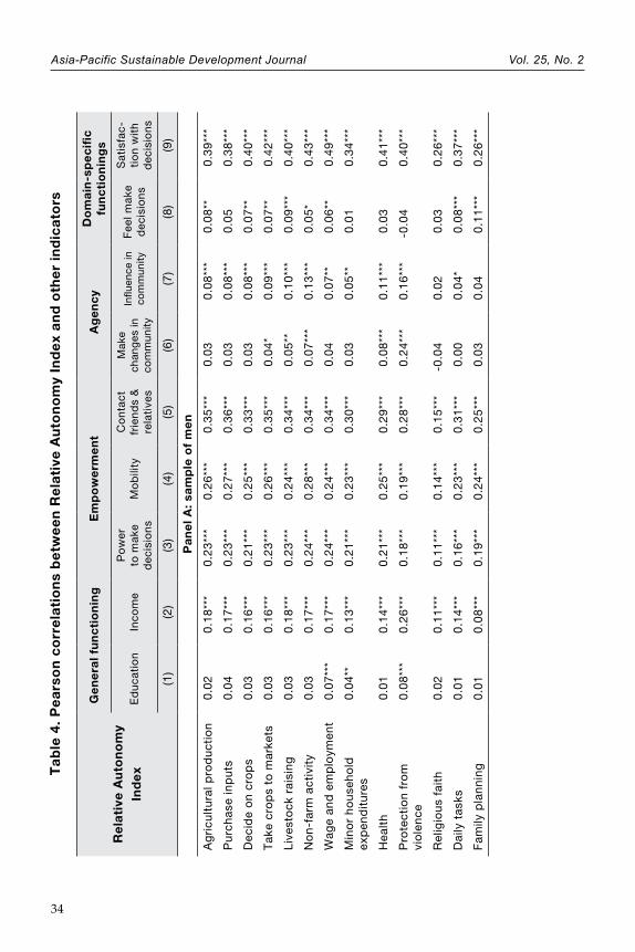
Asia-Pacific Sustainable Development Journal Vol. 25, No. 2
34
Ta
ble
4.
Pe
ars
on
co
rre
lati
on
s b
etw
ee
n R
ela
tive
Au
ton
om
y In
de
x a
nd
oth
er
ind
ica
tors
Re
lati
ve A
uto
no
my
Ind
ex
Ge
ne
ral f
un
cti
on
ing
E
mp
ow
erm
en
tA
ge
nc
yD
om
ain
-sp
ec
ific
fu
nc
tio
nin
gs
Ed
uca
tio
nIn
com
eP
ow
er
to m
ake
dec
isio
ns
Mo
bili
tyC
on
tact
fr
ien
ds
&
rela
tive
s
Mak
e ch
ang
es in
co
mm
unity
Influ
ence
in
com
mun
ityF
eel m
ake
dec
isio
ns
Sat
isfa
c-ti
on
wit
h d
ecis
ion
s
(1)
(2)
(3)
(4)
(5)
(6)
(7)
(8)
(9)
Pa
ne
l A:
sam
ple
of
me
n
Ag
ricu
ltu
ral p
rod
uct
ion
0.0
20
.18
***
0.2
3**
*0
.26
***
0.3
5**
*0
.03
0.0
8**
*0
.08
**0
.39
***
Pu
rch
ase
inp
uts
0.0
40
.17
***
0.2
3**
*0
.27
***
0.3
6**
*0
.03
0.0
8**
*0
.05
0.3
8**
*
Dec
ide
on
cro
ps
0.0
30
.16
***
0.2
1**
*0
.25
***
0.3
3**
*0
.03
0.0
8**
*0
.07
**0
.40
***
Tak
e cr
op
s to
mar
kets
0.0
30
.16
***
0.2
3**
*0
.26
***
0.3
5**
*0
.04
*0
.09
***
0.0
7**
0.4
2**
*
Liv
esto
ck r
aisi
ng
0.0
30
.18
***
0.2
3**
*0
.24
***
0.3
4**
*0
.05
**0
.10
***
0.0
9**
*0
.40
***
No
n-f
arm
act
ivit
y0
.03
0.1
7**
*0
.24
***
0.2
8**
*0
.34
***
0.0
7**
*0
.13
***
0.0
5*
0.4
3**
*
Wag
e an
d e
mp
loym
ent
0.0
7**
*0
.17
***
0.2
4**
*0
.24
***
0.3
4**
*0
.04
0.0
7**
0.0
6**
0.4
9**
*
Min
or
ho
use
ho
ld
exp
end
itu
res
0.0
4**
0.1
3**
*0
.21
***
0.2
3**
* 0
.30
***
0.0
30
.05
**0
.01
0.3
4**
*
Hea
lth
0.0
10
.14
***
0.2
1**
*0
.25
***
0.2
9**
*0
.08
***
0.1
1**
*0
.03
0.4
1**
*
Pro
tect
ion
fro
m
vio
len
ce0
.08
***
0.2
6**
*0
.18
***
0.1
9**
*0
.28
***
0.2
4**
*0
.16
***
-0.0
40
.40
***
Rel
igio
us
fait
h 0
.02
0.1
1**
*0
.11
***
0.1
4**
*0
.15
***
-0.0
40
.02
0.0
30
.26
***
Dai
ly t
asks
0.0
10
.14
***
0.1
6**
*0
.23
***
0.3
1**
*0
.00
0.0
4*
0.0
8**
*0
.37
***
Fam
ily p
lan
nin
g0
.01
0.0
8**
*0
.19
***
0.2
4**
*0
.25
***
0.0
30
.04
0.1
1**
*0
.26
***

Measuring autonomy: evidence from Bangladesh
35
Re
lati
ve A
uto
no
my
Ind
ex
Ge
ne
ral f
un
cti
on
ing
E
mp
ow
erm
en
tA
ge
nc
yD
om
ain
-sp
ec
ific
fu
nc
tio
nin
gs
Ed
uca
tio
nIn
com
eP
ow
er
to m
ake
dec
isio
ns
Mo
bili
tyC
on
tact
fr
ien
ds
&
rela
tive
s
Mak
e ch
ang
es in
co
mm
unity
Influ
ence
in
com
mun
ityF
eel m
ake
dec
isio
ns
Sat
isfa
c-ti
on
wit
h d
ecis
ion
s
(1)
(2)
(3)
(4)
(5)
(6)
(7)
(8)
(9)
Pa
ne
l B:
sam
ple
of
wo
me
n
Ag
ricu
ltu
ral p
rod
uct
ion
0.0
5**
0.0
7**
0.1
8**
*0
.15
***
0.1
4**
*0
.08
**0
.10
***
0.0
7**
0.2
8**
*
Pu
rch
ase
inp
uts
0.0
5**
0.0
9**
*0
.20
***
0.1
8**
*0
.17
***
0.0
7**
0.1
2**
*0
.08
***
0.3
0**
*
Dec
ide
on
cro
ps
0.0
6**
0.0
8**
*0
.19
***
0.1
5**
*0
.15
***
0.0
7**
0.1
1**
*0
.08
***
0.3
0**
*
Tak
e cr
op
s to
mar
kets
0.0
5*
0.1
0**
*0
.20
***
0.1
5**
*0
.17
***
0.0
8**
0.1
1**
*0
.09
***
0.3
0**
*
Liv
esto
ck r
aisi
ng
0.0
10
.07
***
0.1
3**
*0
.09
***
0.1
0**
*0
.07
**0
.11
***
0.1
0**
*0
.33
***
No
n-f
arm
act
ivit
y0
.06
*0
.12
***
0.1
5**
*0
.15
***
0.1
3**
*0
.08
*0
.10
**0
.10
***
0.3
2**
*
Wag
e an
d e
mp
loym
ent
0.0
40
.05
0.1
0**
*0
.11
***
0.1
1**
*-0
.01
0.0
30
.04
0.3
0**
*
Min
or
ho
use
ho
ld
exp
end
itu
res
0.0
20
.05
**0
.14
***
0.1
0**
*0
.08
***
0.0
40
.08
***
0.0
7**
*0
.33
***
Hea
lth
0.0
20
.06
**0
.15
***
0.1
2**
*0
.11
***
0.0
5*
0.1
0**
*0
.03
0.3
2**
*
Pro
tect
ion
fro
m
vio
len
ce0
.08
**0
.03
0.1
1**
0.0
9*
0.1
8**
*-0
.03
-0.0
20
.11
***
0.3
7**
*
Rel
igio
us
fait
h 0
.06
**0
.09
***
0.0
9**
0.0
7**
0.0
30
.07
**0
.06
**0
.04
0.3
3**
*
Dai
ly t
asks
0.0
20
.09
***
0.0
9**
*0
.07
***
0.0
7**
*0
.06
**0
.07
***
0.0
8**
*0
.30
***
Fam
ily p
lan
nin
g0
.04
**0
.06
**0
.12
***
0.0
7**
*0
.06
**0
.06
**0
.12
***
0.0
10
.33
***
No
te:
***
p<
0.01
, **
p<
0.05
, *p
<0.
1".

Asia-Pacific Sustainable Development Journal Vol. 25, No. 2
36
We examine the Pearson correlation coefficients, which allow us to account for the survey design (table 4). We report the Spearman and Kendall tau rank correlation coefficients in the online appendix. Contrary to what is commonly assumed, we find that autonomy is not highly correlated with education – although the coefficient is significant in some domains, it never goes beyond 0.08. Autonomy is also not strongly correlated with expenditure quintile. Although the correlation coefficient is almost always statistically significant, the magnitude is relatively small. The correlation between autonomy and income is consistently higher among men (average of 0.16 across domains) than among women (average of 0.07).
The three indicators of empowerment are correlated with autonomy in practically all domains. Again, the magnitude of this correlation is, on average, higher in the sample of men than in the sample of women – and again, the correlation levels are modest. This time, correlation levels for men between autonomy and empowerment reach 0.24 for decision-making; 0.28 for mobility; and 0.35 for contact friends and relatives. Women’s correlations are lower and more uniform across the empowerment indicators, and never above 0.20. The correlations with the indicators of agency are generally relatively weak and not significant in all domains.
We find that the RAI and satisfaction with decisions made are slightly more strongly correlated: the average correlation coefficient across domains is 0.38 for men and 0.32 for women. This means that, on average, individuals with higher autonomy are more satisfied with their decisions; however, the level of correlation is still relatively low.
On the other hand, the question of whether the respondent either makes a decision in the domain or feels she could make a decision if she wished – which is an improvement on the standard decision-making questions that are often used to proxy empowerment – has low correlations for both men and women across all domains. In all but two cases correlations are 0.1 or under.
In summary, the two indicators that are slightly more correlated with individuals’ relative autonomy, consistently across gender, are the domain-specific indicator of satisfaction with decisions made and the general indicator of satisfaction with “power to make important decisions that change one’s course of life”, but even these correlation values are relatively low.
Regression analysis
The correlation analysis provides only a rudimentary view of the relationship between different indicators, as it ignores both interactions between variables and non-linear relations. We use regression analysis to examine more formally the relationship between autonomy and other individual and household characteristics, and to investigate the extent to which other indicators could be used as proxies for individual relative autonomy in Bangladesh.

Measuring autonomy: evidence from Bangladesh
37
5.2.1 Empirical specification
We start by estimating the following equation:
RAIi = β0+β1Xi+β2Fi+β3Hi+εi (1)
where RAIij is individual i’s Relative Autonomy Index in domain j, Xi is a vector of individual and household demographic characteristics (e.g. age, marital status, and number of household members), Fi is a vector of indicators of an individual’s general functionings (e.g. years of schooling), Hi is a vector of indicators of housing quality and assets (e.g. improved sanitation, access to drinking water, ownership of assets), and εi is the error term. A list of the covariates and the respective descriptive statistics are included in the online appendix.
In a second round of regressions we include an additional set of explanatory variables, Zi (potential proxies for the RAI), to see how these are associated with autonomy, after we control for the individual and household’s characteristics.
RAIij = β0+β1Xi+β2Fi+β3Hi+β4Zi+εi (2)
The summary statistics of all the variables used are presented in table A.3 in the online appendix.
The equations are estimated using a linear model,14 separately for men and women,15 and taking account of the complex survey design. Division dummies are included in all regressions to control for location specific effects.16
Results
Estimates of equation (1) for the Relative Autonomy Index (RAI) in domains of “agriculture production”, “livestock raising”, “non-farm business” and “protection from violence” are presented in table 5. We selected these domains because they cover a broad spectrum of activities (including the main occupation of men and women in the sample) and allow us to illustrate our main conclusions.
14 The Relative Autonomy Index is a Likert Scale. So, it can be analysed as an interval scale (Allen and Seaman, 2007; Brown, 2011; Carifio and Perla, 2007).
15 Otherwise, as there is a male and female from each household, the errors are likely to be correlated.16 We also estimated the equations using an ordered probit model, as a robustness check. The
conclusions did not change. These estimates are included in the online appendix.

Asia-Pacific Sustainable Development Journal Vol. 25, No. 2
38
Ta
ble
5.
Est
ima
tes
of
eq
ua
tio
n (
1) u
sin
g a
lin
ea
r re
gre
ssio
n m
od
el
Va
ria
ble
sD
om
ain
s
Ag
ric
ult
ure
p
rod
uc
tio
nL
ive
sto
ck
ra
isin
gN
on
-fa
rmin
g
bu
sin
ess
ac
tivi
tyP
rote
cti
on
fro
m
vio
len
ce
Me
nW
om
en
Me
nW
om
en
Me
nW
om
en
Me
nW
om
en
(1)
(2)
(3)
(4)
(5)
(6)
(7)
(8)
Ag
e0
.00
80
.00
70
.00
90
.00
1-0
.00
2-0
.00
10
.00
10
.01
3
(0.0
06
)(0
.00
9)
(0.0
06
)(0
.00
8)
(0.0
08
)(0
.01
1)
(0.0
07
)(0
.01
0)
Ho
use
ho
ld h
ead
0.2
05
0.0
70
-0.1
53
0.0
82
0.7
54
0.4
84
0.3
06
0.7
61
***
(0.5
62
)(0
.26
9)
(0.4
70
)(0
.24
5)
(0.5
45
)(0
.39
8)
(0.5
61
)(0
.22
5)
Nu
mb
er o
f h
ou
seh
old
mem
ber
s0
.09
6**
0.0
26
0.0
57
-0.0
84
0.1
74
***
0.0
33
0.0
93
-0.0
33
(0.0
48
)(0
.05
4)
(0.0
57
)(0
.05
6)
(0.0
52
)(0
.07
4)
(0.0
61
)(0
.06
6)
Nu
mb
er o
f m
emb
ers
<6
0.1
98
*0
.19
60
.26
2**
0.1
14
-0.1
00
-0.4
16
***
0.0
07
0.2
48
(0.1
11
)(0
.12
2)
(0.1
17
)(0
.11
9)
(0.1
29
)(0
.13
0)
(0.1
40
)(0
.15
1)
Yea
rs o
f ed
uca
tio
n-0
.02
10
.02
3-0
.03
8*
-0.0
13
-0.0
38
0.0
08
-0.0
00
0.0
72
**
(0.0
20
)(0
.02
6)
(0.0
22
)(0
.02
4)
(0.0
24
)(0
.03
2)
(0.0
21
)(0
.03
0)
Occ
up
atio
n in
ag
ricu
ltu
re0
.28
7-0
.71
9**
*-0
.03
3-0
.55
4**
*0
.65
1-0
.35
5*
-0.2
27
-0.5
61
**
(0.5
96
)(0
.18
5)
(0.6
48
)(0
.16
7)
(0.6
66
)(0
.21
1)
(0.7
54
)(0
.22
2)
San
itat
ion
-0.5
39
***
0.3
48
*-0
.25
80
.46
0**
-0.1
54
0.2
83
-1.0
53
***
0.4
76
*
(0.1
92
)(0
.18
6)
(0.2
28
)(0
.19
5)
(0.2
36
)(0
.23
2)
(0.2
89
)(0
.24
5)
Co
oki
ng
fu
el-1
.05
4**
-0.6
30
-0.0
87
-0.2
10
-1.1
61
**-0
.13
9-0
.41
7-0
.85
5
(0.4
56
)(0
.42
2)
(0.4
85
)(0
.39
8)
(0.5
58
)(0
.57
8)
(0.5
37
)(0
.54
7)
Ass
ets
- ac
cess
to
info
rmat
ion
0.4
11
**0
.23
50
.12
00
.14
10
.31
90
.52
0**
0.0
36
0.1
81
(0.1
91
)(0
.20
9)
(0.2
01
)(0
.18
8)
(0.2
00
)(0
.24
8)
(0.1
89
)(0
.24
0)
Ass
ets
- su
pp
ort
to
mo
bili
ty0
.12
5-0
.17
60
.14
80
.04
5-0
.00
10
.45
3**
-0.0
39
0.3
89
*
(0.1
55
)(0
.15
5)
(0.1
68
)(0
.15
9)
(0.1
75
)(0
.19
3)
(0.1
65
)(0
.22
0)

Measuring autonomy: evidence from Bangladesh
39
Va
ria
ble
sD
om
ain
s
Ag
ric
ult
ure
p
rod
uc
tio
nL
ive
sto
ck
ra
isin
gN
on
-fa
rmin
g
bu
sin
ess
ac
tivi
tyP
rote
cti
on
fro
m
vio
len
ce
Me
nW
om
en
Me
nW
om
en
Me
nW
om
en
Me
nW
om
en
(1)
(2)
(3)
(4)
(5)
(6)
(7)
(8)
Ass
ets
- su
pp
ort
to
live
liho
od
0.2
30
0.1
69
0.6
58
***
0.7
68
***
-0.0
29
0.0
87
-0.1
45
0.4
00
*
(0.1
73
)(0
.16
6)
(0.2
41
)(0
.20
6)
(0.1
77
)(0
.20
8)
(0.2
00
)(0
.22
1)
Ho
use
ho
ld e
xpen
dit
ure
per
cap
ita
0.3
40
***
0.0
28
0.3
23
***
-0.0
25
0.3
06
***
-0.0
13
0.4
71
***
-0.1
74
**
(0.0
64
)(0
.06
6)
(0.0
71
)(0
.06
7)
(0.0
69
)(0
.08
4)
(0.0
82
)(0
.07
5)
Bar
isal
-1.2
19
**0
.50
6-1
.12
4**
-3.0
60
***
-1.8
06
***
0.5
00
-1.3
55
**0
.66
0
(0.5
80
)(0
.82
7)
(0.5
70
)(0
.69
0)
(0.6
10
)(0
.94
5)
(0.5
28
)(0
.57
3)
Ch
itta
go
ng
-0.0
54
-1.2
10
***
0.1
59
-1.7
86
***
0.0
29
-1.2
83
**-0
.23
5-2
.50
7**
*
(0.5
11
)(0
.39
5)
(0.5
16
)(0
.46
1)
(0.4
50
)(0
.53
1)
(0.6
20
)(0
.43
1)
Kh
uln
a1
.21
0**
*1
.02
3**
*1
.42
9**
*0
.13
01
.48
0**
*1
.37
4**
*0
.42
8-0
.14
6
(0.3
85
)(0
.35
4)
(0.3
81
)(0
.34
2)
(0.3
86
)(0
.44
8)
(0.4
07
)(0
.43
1)
Raj
shah
i-1
.77
5**
*-0
.76
8-1
.85
6**
*-2
.23
1**
*-2
.54
2**
*-1
.29
5*
-3.4
20
***
-1.3
42
*
(0.4
81
)(0
.63
8)
(0.5
03
)(0
.60
1)
(0.5
01
)(0
.70
2)
(0.4
09
)(0
.74
0)
Ran
gp
ur
-2.6
96
***
-1.3
33
***
-2.2
74
***
-2.4
60
***
-2.9
69
***
-2.0
13
***
-3.2
06
***
-3.3
48
***
(0.3
75
)(0
.35
8)
(0.4
52
)(0
.35
4)
(0.4
19
)(0
.43
2)
(0.3
78
)(0
.33
5)
Syl
het
0.0
45
-0.9
94
**0
.13
5-1
.23
7**
-0.3
75
-1.4
71
**-2
.17
8**
*0
.43
0
(0.4
11
)(0
.50
4)
(0.3
90
)(0
.54
6)
(0.4
29
)(0
.65
5)
(0.5
69
)(0
.43
1)
Co
nst
ant
2.2
01
***
3.6
42
***
2.0
92
***
4.8
37
***
3.2
93
***
3.6
43
***
1.6
89
**4
.93
2**
*
(0.5
28
)(0
.68
0)
(0.6
56
)(0
.62
7)
(0.6
18
)(1
.17
9)
(0.7
21
)(0
.73
8)
F-s
tati
stic
12
.9**
*5
.7**
*8
.0**
*7
.1**
*9
.8**
*9
.3**
*1
9.2
***
14
.9**
*
R-s
qu
ared
0.1
77
0.0
78
0.1
65
0.1
31
0.2
05
0.1
32
0.2
60
0.2
01
Nu
mb
er o
f o
bse
rvat
ion
s2
88
22
63
62
80
93
23
12
22
21
60
71
66
01
52
4
No
te:
The
tab
le d
oes
not
incl
ude
the
estim
ates
of
exp
lana
tory
var
iab
les
that
are
not
sig
nific
ant
in a
ny o
f th
e re
gres
sion
s p
rese
nted
, na
mel
y: o
ccup
atio
n of
hous
ehol
d h
ead
, nu
triti
on a
nd d
rinki
ng w
ater
. **
* p
<0.
01,
** p
<0.
05,
* p
<0.
1.

Asia-Pacific Sustainable Development Journal Vol. 25, No. 2
40
Three general features become apparent when we look at these tables. First, men’s and women’s relative autonomy seems to be determined by different factors. Second, geographical location, which may proxy different cultural norms in each of Bangladesh’s divisions, affects the autonomy of both men and women. Third, the factors that determine relative autonomy vary across domains of decision-making.
Differences across gender. Men’s autonomy is positively associated with income. The coefficient of the quintile of per capita expenditure is significant in all regressions of men’s RAI. On the other hand, this coefficient is not significant in any of the regressions of women’s RAI, except in “protection from violence”, where the coefficient is negative. However, the negative sign on protection from violence may highlight the possibility that domestic violence (which is the likely form of violence to which women are more exposed in Bangladesh) does not decrease with income.
Women’s relative autonomy, on the other hand, is associated with their occupation and sector of work. The results suggest that women engaged in activities related to agriculture tend to have lower levels of autonomy than women engaged in other activities. This relationship is significant at the 1 per cent level in all domains, except “non-farming business activity”. The occupation of most women in rural Bangladesh is either livestock/poultry raising (50 per cent of the sample) – here classified as related to agriculture – or housewife (42 per cent). Housewives thus appear to have higher autonomy than other women, possibly because they may have greater decision-making power within the domestic sphere, compared to agriculture where men typically make most of the decisions.
Less important, but intriguing, we find that sanitation tends to be negatively associated with men’s autonomy, but positively associated with women’s RAI. It is possible that having better sanitation facilities on one’s homestead reduces women’s vulnerability in terms of having to use facilities outside, but this effect does not hold for men.17 Another possible explanation is that improved sanitation might reduce the number of illness episodes in the household and be associated with easier access to water, thereby reducing women’s unpaid care and domestic work.
Geographical location. The high significance of the location dummies suggests that, after controlling for income distribution, basic housing conditions and individuals’ characteristics, there are (unobservable) local factors that have a strong effect on individuals’ autonomy. However, as location dummies capture differences in social norms and economic conditions that may have offsetting effects, these coefficients need to be interpreted carefully.
17 Indeed, in some parts of South Asia, a husband’s assurance that the home to which a bride is moving has its own toilet has become a condition for marriage.

Measuring autonomy: evidence from Bangladesh
41
Determinants of autonomy in specific domains. The pattern of determinants of women’s autonomy in the domain of “protection from violence” is particularly interesting. Women’s education is not significantly associated with autonomy in any other domain. This is an important result, given the high rates of intimate partner violence in Bangladesh: increasing women’s education thus continues to be an important policy priority for women’s overall empowerment and welfare.18 Being the household head is also associated with women’s autonomy only in this domain, possibly because being a female head of household often results from widowhood or divorce, and implies the absence of a husband and in-laws who might perpetuate domestic violence.
It is noteworthy that ownership of specific assets affects women’s autonomy in different domains. For instance, assets related to access to information and support to mobility seem to have a positive impact on women’s autonomy in the domain of “non-farming business activity”. Assets to support livelihoods also have a positive impact on women’s autonomy in protection from violence, which is consistent with findings from India that asset ownership protects against domestic violence (Panda and Agarwal, 2005). In contrast to income, assets, particularly those related to information, mobility and livelihood, thus appear to have a positive impact on women’s autonomy. These results are potentially relevant to programmes that seek to increase women’s control of assets.
The set of variables that are significantly correlated with the Relative Autonomy Index varies across domains. This evidence supports the hypothesis that autonomy is domain-specific and, therefore, it should be measured separately in different domains.
The analysis above has shown that neither age, education nor income are suitable proxies for relative autonomy of men and women. Now we investigate if the indicators on decision-making are valid candidates.
18 Unfortunately, we do not have information on the “forms” that violence takes. For instance, withdrawal of financial support and physical abuse are very distinct forms of violence and most likely have different implications for autonomy.
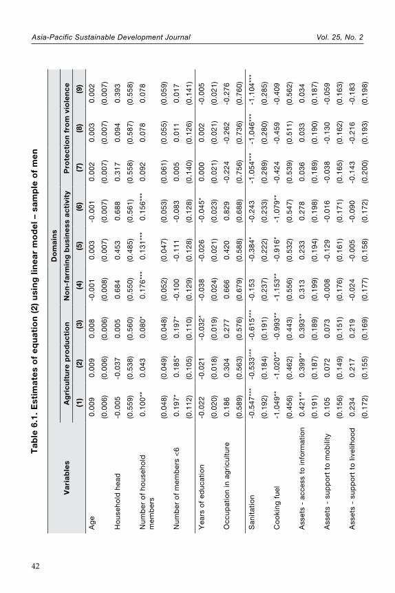
Asia-Pacific Sustainable Development Journal Vol. 25, No. 2
42
Ta
ble
6.1
. E
stim
ate
s o
f e
qu
ati
on
(2)
usi
ng
lin
ea
r m
od
el –
sa
mp
le o
f m
en
Do
ma
ins
Va
ria
ble
sA
gri
cu
ltu
re p
rod
uc
tio
nN
on
-fa
rmin
g b
usi
ne
ss a
cti
vity
Pro
tec
tio
n f
rom
vio
len
ce
(1)
(2)
(3)
(4)
(5)
(6)
(7)
(8)
(9)
Ag
e0
.00
90
.00
90
.00
8-0
.00
10
.00
3-0
.00
10
.00
20
.00
30
.00
2
(0.0
06
)(0
.00
6)
(0.0
06
)(0
.00
8)
(0.0
07
)(0
.00
7)
(0.0
07
)(0
.00
7)
(0.0
07
)
Ho
use
ho
ld h
ead
-0.0
05
-0.0
37
0.0
05
0.6
84
0.4
53
0.6
88
0.3
17
0.0
94
0.3
93
(0.5
59
)(0
.53
8)
(0.5
60
)(0
.55
0)
(0.4
85
)(0
.56
1)
(0.5
58
)(0
.58
7)
(0.5
58
)
Nu
mb
er o
f h
ou
seh
old
m
emb
ers
0.1
00
**0
.04
30
.08
0*
0.1
76
***
0.1
31
***
0.1
56
***
0.0
92
0.0
78
0.0
78
(0.0
48
)(0
.04
9)
(0.0
48
)(0
.05
2)
(0.0
47
)(0
.05
3)
(0.0
61
)(0
.05
5)
(0.0
59
)
Nu
mb
er o
f m
emb
ers
<6
0.1
97
*0
.18
5*
0.1
97
*-0
.10
0-0
.11
1-0
.08
30
.00
50
.01
10
.01
7
(0.1
12
)(0
.10
5)
(0.1
10
)(0
.12
9)
(0.1
28
)(0
.12
8)
(0.1
40
)(0
.12
6)
(0.1
41
)
Yea
rs o
f ed
uca
tio
n-0
.02
2-0
.02
1-0
.03
2*
-0.0
38
-0.0
26
-0.0
45
*0
.00
00
.00
2-0
.00
5
(0.0
20
)(0
.01
8)
(0.0
19
)(0
.02
4)
(0.0
21
)(0
.02
3)
(0.0
21
)(0
.02
1)
(0.0
21
)
Occ
up
atio
n in
ag
ricu
ltu
re0
.18
60
.30
40
.27
70
.66
60
.42
00
.82
9-0
.22
4-0
.26
2-0
.27
6
(0.5
89
)(0
.56
3)
(0.5
76
)(0
.67
9)
(0.5
88
)(0
.68
8)
(0.7
56
)(0
.73
6)
(0.7
60
)
San
itat
ion
-0.5
47
***
-0.5
33
***
-0.6
15
***
-0.1
53
-0.3
84
*-0
.24
3-1
.05
4**
*-1
.04
6**
*-1
.10
4**
*
(0.1
92
)(0
.18
4)
(0.1
91
)(0
.23
7)
(0.2
22
)(0
.23
3)
(0.2
89
)(0
.28
0)
(0.2
85
)
Co
oki
ng
fu
el-1
.04
9**
-1.0
20
**-0
.99
3**
-1.1
53
**-0
.91
6*
-1.0
79
**-0
.42
4-0
.45
9-0
.40
9
(0.4
56
)(0
.46
2)
(0.4
43
)(0
.55
6)
(0.5
32
)(0
.54
7)
(0.5
39
)(0
.51
1)
(0.5
62
)
Ass
ets
- ac
cess
to
info
rmat
ion
0.4
21
**0
.39
9**
0.3
93
**0
.31
30
.23
30
.27
80
.03
60
.03
30
.03
4
(0.1
91
)(0
.18
7)
(0.1
89
)(0
.19
9)
(0.1
94
)(0
.19
8)
(0.1
89
)(0
.19
0)
(0.1
87
)
Ass
ets
- su
pp
ort
to
mo
bili
ty0
.10
50
.07
20
.07
3-0
.00
8-0
.12
9-0
.01
6-0
.03
8-0
.13
0-0
.05
9
(0.1
56
)(0
.14
9)
(0.1
51
)(0
.17
6)
(0.1
61
)(0
.17
1)
(0.1
65
)(0
.16
2)
(0.1
63
)
Ass
ets
- su
pp
ort
to
live
liho
od
0.2
34
0.2
17
0.2
19
-0.0
24
-0.0
05
-0.0
90
-0.1
43
-0.2
16
-0.1
83
(0.1
72
)(0
.15
5)
(0.1
69
)(0
.17
7)
(0.1
58
)(0
.17
2)
(0.2
00
)(0
.19
3)
(0.1
98
)

Measuring autonomy: evidence from Bangladesh
43
Do
ma
ins
Va
ria
ble
sA
gri
cu
ltu
re p
rod
uc
tio
nN
on
-fa
rmin
g b
usi
ne
ss a
cti
vity
Pro
tec
tio
n f
rom
vio
len
ce
(1)
(2)
(3)
(4)
(5)
(6)
(7)
(8)
(9)
Ho
use
ho
ld e
xpen
dit
ure
per
ca
pit
a0
.34
1**
*0
.22
8**
*0
.29
6**
*0
.30
2**
*0
.20
2**
*0
.25
7**
*0
.46
9**
*0
.42
0**
*0
.44
5**
*
(0.0
64
)(0
.06
1)
(0.0
62
)(0
.07
0)
(0.0
64
)(0
.07
0)
(0.0
81
)(0
.07
8)
(0.0
80
)
Bar
isal
-1.2
62
**-1
.47
6**
*-1
.30
4**
-1.8
26
***
-2.0
76
***
-1.9
02
***
-1.3
46
**-1
.55
2**
*-1
.39
9**
*
(0.5
81
)(0
.56
3)
(0.5
44
)(0
.61
2)
(0.6
04
)(0
.56
4)
(0.5
34
)(0
.53
7)
(0.5
17
)
Ch
itta
go
ng
-0.1
00
-0.0
57
-0.0
87
0.0
06
0.0
03
-0.0
05
-0.2
32
-0.2
73
-0.1
51
(0.5
12
)(0
.46
5)
(0.5
01
)(0
.45
2)
(0.4
01
)(0
.44
4)
(0.6
21
)(0
.57
0)
(0.6
20
)
Kh
uln
a1
.20
4**
*0
.97
1**
1.0
59
***
1.4
70
***
1.1
01
***
1.3
32
***
0.4
24
0.4
72
0.3
99
(0.3
88
)(0
.38
8)
(0.3
76
)(0
.38
7)
(0.3
70
)(0
.37
5)
(0.4
07
)(0
.39
8)
(0.4
06
)
Raj
shah
i-1
.70
8**
*-0
.93
8**
-1.5
46
***
-2.5
40
***
-1.7
55
***
-2.3
23
***
-3.4
23
***
-2.7
44
***
-3.3
13
***
(0.4
69
)(0
.44
4)
(0.4
61
)(0
.50
2)
(0.4
52
)(0
.49
3)
(0.4
04
)(0
.40
0)
(0.4
11
)
Ran
gp
ur
-2.6
98
***
-2.2
63
***
-2.4
57
***
-2.9
59
***
-2.2
23
***
-2.7
16
***
-3.2
04
***
-2.5
08
***
-3.1
00
***
(0.3
73
)(0
.35
5)
(0.3
90
)(0
.42
1)
(0.3
68
)(0
.43
1)
(0.3
78
)(0
.37
7)
(0.3
85
)
Syl
het
0.0
27
0.1
72
0.3
51
-0.3
98
-0.2
66
0.0
03
-2.1
79
***
-1.4
75
***
-1.9
04
***
(0.4
08
)(0
.36
5)
(0.3
97
)(0
.42
8)
(0.3
74
)(0
.43
3)
(0.5
68
)(0
.53
5)
(0.5
80
)
Fee
l can
mak
e d
ecis
ion
s0
.65
9**
0.3
91
0.5
92
**0
.34
20
.23
40
.29
6-0
.05
9-0
.10
4-0
.07
2
(0.2
82
)(0
.29
7)
(0.2
82
)(0
.29
0)
(0.2
64
)(0
.28
0)
(0.2
37
)(0
.23
0)
(0.2
38
)
Sat
isfa
ctio
n w
ith
dec
isio
ns
-1
.09
6**
*-
-1
.29
3**
*-
-0
.94
9**
*-
-(0
.12
4)
--
(0.1
28
)-
-(0
.14
7)
-
Po
wer
to
mak
e d
ecis
ion
s-
-0
.24
7**
*-
-0
.28
4**
*-
-0
.14
6**
--
(0.0
46
)-
-(0
.05
1)
--
(0.0
61
)
Co
nst
ant
1.7
91
***
-1.9
91
***
0.6
08
3.0
69
***
-2.0
63
***
1.6
08
**1
.72
6**
-1.7
99
**0
.92
1
(0.5
41
)(0
.69
8)
(0.5
72
)(0
.63
8)
(0.7
45
)(0
.67
5)
(0.7
10
)(0
.81
7)
(0.7
64
)

Asia-Pacific Sustainable Development Journal Vol. 25, No. 2
44
Do
ma
ins
Va
ria
ble
sA
gri
cu
ltu
re p
rod
uc
tio
nN
on
-fa
rmin
g b
usi
ne
ss a
cti
vity
Pro
tec
tio
n f
rom
vio
len
ce
(1)
(2)
(3)
(4)
(5)
(6)
(7)
(8)
(9)
F-s
tati
stic
13
.06
***
17
.05
***
13
.60
***
9.4
2**
*2
1.5
3**
*1
2.4
3**
*1
8.6
7**
*2
4.4
1**
*1
8.1
0**
*
R-s
qu
ared
0.1
80
0.2
48
0.1
99
0.2
05
0.2
88
0.2
27
0.2
60
0.3
09
0.2
66
Nu
mb
er o
f o
bse
rvat
ion
s2
88
22
87
62
88
22
22
22
21
52
22
21
66
01
64
31
66
0
No
te:
The
tab
le d
oes
not
incl
ude
the
estim
ates
of
exp
lana
tory
var
iab
les
that
are
not
sig
nific
ant
in a
ny o
f th
e re
gres
sion
s p
rese
nted
, na
mel
y: o
ccup
atio
n of
hous
ehol
d h
ead
, nu
triti
on a
nd d
rinki
ng w
ater
. **
* p
<0.
01,
** p
<0.
05,
* p
<0.
1.
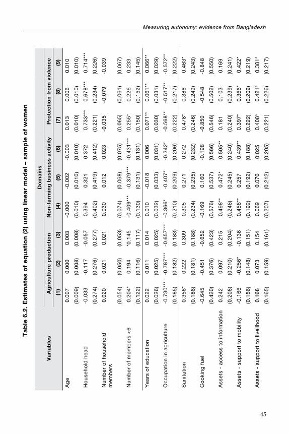
Measuring autonomy: evidence from Bangladesh
45
Ta
ble
6.2
. E
stim
ate
s o
f e
qu
ati
on
(2)
usi
ng
lin
ea
r m
od
el –
sa
mp
le o
f w
om
en
Do
ma
ins
Va
ria
ble
sA
gri
cu
ltu
re p
rod
uc
tio
nN
on
-fa
rmin
g b
usi
ne
ss a
cti
vity
Pro
tec
tio
n f
rom
vio
len
ce
(1)
(2)
(3)
(4)
(5)
(6)
(7)
(8)
(9)
Ag
e0
.00
70
.00
00
.00
3-0
.00
0-0
.00
2-0
.00
30
.01
30
.00
60
.01
0
(0.0
09
)(0
.00
8)
(0.0
08
)(0
.01
0)
(0.0
10
)(0
.01
0)
(0.0
10
)(0
.01
0)
(0.0
10
)
Ho
use
ho
ld h
ead
-0.0
33
-0.1
17
-0.0
57
0.3
94
0.3
21
0.3
72
0.7
33
***
0.6
78
***
0.7
14
***
(0.2
74
)(0
.27
6)
(0.2
77
)(0
.40
2)
(0.4
19
)(0
.41
2)
(0.2
21
)(0
.23
4)
(0.2
26
)
Nu
mb
er o
f h
ou
seh
old
m
emb
ers
0.0
20
0.0
21
0.0
21
0.0
30
0.0
12
0.0
23
-0.0
35
-0.0
79
-0.0
39
(0.0
54
)(0
.05
0)
(0.0
53
)(0
.07
4)
(0.0
68
)(0
.07
5)
(0.0
65
)(0
.06
1)
(0.0
67
)
Nu
mb
er o
f m
emb
ers
<6
0.2
04
*0
.19
4*0
.14
5-0
.40
9**
*-0
.37
9**
*-0
.43
1**
*0
.25
5*
0.2
26
0.2
33
(0.1
22
)(0
.11
6)
(0.1
17
)(0
.13
0)
(0.1
31
)(0
.13
1)
(0.1
50
)(0
.15
2)
(0.1
45
)
Yea
rs o
f ed
uca
tio
n0
.02
20
.01
10
.01
40
.01
0-0
.01
80
.00
60
.07
1**
0.0
61
**0
.06
6**
(0.0
26
)(0
.02
5)
(0.0
25
)(0
.03
2)
(0.0
33
)(0
.03
1)
(0.0
30
)(0
.03
1)
(0.0
29
)
Occ
up
atio
n in
ag
ricu
ltu
re-0
.73
0**
*-0
.78
7**
*-0
.65
7**
*-0
.36
6*
-0.4
07
*-0
.34
2*
-0.5
68
**-0
.51
7**
-0.5
72
**
(0.1
85
)(0
.18
2)
(0.1
83
)(0
.21
0)
(0.2
09
)(0
.20
6)
(0.2
22
)(0
.21
7)
(0.2
22
)
San
itat
ion
0.3
56
*0
.22
20
.30
90
.30
50
.27
10
.27
20
.47
8*
0.3
86
0.4
63
*
(0.1
86
)(0
.18
1)
(0.1
88
)(0
.23
4)
(0.2
35
)(0
.23
2)
(0.2
46
)(0
.24
9)
(0.2
43
)
Co
oki
ng
fu
el-0
.64
5-0
.45
1-0
.65
2-0
.16
90
.16
0-0
.19
8-0
.85
0-0
.54
8-0
.84
8
(0.4
20
)(0
.37
6)
(0.4
23
)(0
.57
6)
(0.5
37
)(0
.56
6)
(0.5
46
)(0
.50
2)
(0.5
50
)
Ass
ets
- ac
cess
to
info
rmat
ion
0.2
42
0.0
97
0.2
15
0.4
98
**0
.47
2*
0.5
05
**0
.18
10
.10
30
.16
9
(0.2
08
)(0
.21
0)
(0.2
04
)(0
.24
6)
(0.2
45
)(0
.24
0)
(0.2
40
)(0
.23
9)
(0.2
41
)
Ass
ets
- su
pp
ort
to
mo
bili
ty-0
.16
6-0
.25
6*
-0.1
36
0.4
58
**0
.25
70
.43
9**
0.3
97
*0
.36
6*
0.4
22
*
(0.1
56
)(0
.14
8)
(0.1
51
)(0
.19
2)
(0.1
92
)(0
.18
8)
(0.2
22
)(0
.20
9)
(0.2
19
)
Ass
ets
- su
pp
ort
to
live
liho
od
0.1
68
0.0
73
0.1
54
0.0
69
0.0
70
0.0
25
0.4
08
*0
.42
1*
0.3
81
*
(0.1
65
)(0
.15
9)
(0.1
61
)(0
.20
7)
(0.2
12
)(0
.20
5)
(0.2
21
)(0
.22
6)
(0.2
17
)

Asia-Pacific Sustainable Development Journal Vol. 25, No. 2
46
Do
ma
ins
Va
ria
ble
sA
gri
cu
ltu
re p
rod
uc
tio
nN
on
-fa
rmin
g b
usi
ne
ss a
cti
vity
Pro
tec
tio
n f
rom
vio
len
ce
(1)
(2)
(3)
(4)
(5)
(6)
(7)
(8)
(9)
Ho
use
ho
ld e
xpen
dit
ure
per
ca
pit
a0
.02
20
.00
3-0
.04
1-0
.02
0-0
.05
6-0
.06
9-0
.17
4**
-0.1
73
**-0
.19
9**
*
(0.0
67
)(0
.06
5)
(0.0
67
)(0
.08
3)
(0.0
82
)(0
.08
5)
(0.0
75
)(0
.07
6)
(0.0
77
)
Bar
isal
0.5
30
0.4
47
0.6
39
0.4
41
0.4
15
0.5
75
0.6
36
-0.1
06
0.6
19
(0.8
28
)(0
.77
4)
(0.8
20
)(0
.94
6)
(0.8
68
)(0
.94
5)
(0.5
76
)(0
.54
0)
(0.5
66
)
Ch
itta
go
ng
-1.1
55
***
-1.3
39
***
-1.1
03
***
-1.2
33
**-1
.39
0**
-1.1
79
**-2
.48
6**
*-2
.80
1**
*-2
.39
3**
*
(0.4
02
)(0
.41
2)
(0.3
96
)(0
.53
6)
(0.5
65
)(0
.53
6)
(0.4
29
)(0
.41
6)
(0.4
19
)
Kh
uln
a1
.03
6**
*0
.78
0**
1.0
25
***
1.3
35
***
1.0
78
**1
.34
0**
*-0
.18
0-0
.74
5**
-0.2
08
(0.3
53
)(0
.34
0)
(0.3
35
)(0
.44
5)
(0.4
38
)(0
.44
7)
(0.4
32
)(0
.34
8)
(0.4
53
)
Raj
shah
i-0
.77
1-0
.71
6-0
.80
5-1
.30
2*
-1.2
21
**-1
.27
1*
-1.3
50
*-1
.68
2**
*-1
.39
4*
(0.6
35
)(0
.56
6)
(0.5
87
)(0
.69
2)
(0.6
22
)(0
.67
9)
(0.7
39
)(0
.59
1)
(0.7
13
)
Ran
gp
ur
-1.2
91
***
-1.1
96
***
-1.3
01
***
-1.9
66
***
-1.7
54
***
-1.9
40
***
-3.3
38
***
-3.0
42
***
-3.3
67
***
(0.3
62
)(0
.35
7)
(0.3
56
)(0
.43
7)
(0.4
21
)(0
.43
7)
(0.3
40
)(0
.39
2)
(0.3
46
)
Syl
het
-0.9
24
*-0
.84
7*
-0.7
67
-1.4
70
**-1
.43
3**
-1.3
09
**0
.40
60
.07
60
.43
9
(0.5
11
)(0
.46
0)
(0.4
94
)(0
.66
6)
(0.6
24
)(0
.66
5)
(0.4
32
)(0
.39
0)
(0.4
40
)
Fee
l can
mak
e d
ecis
ion
s0
.31
6**
0.1
32
0.1
68
0.3
62
*0
.15
30
.29
80
.13
6-0
.07
00
.10
8
(0.1
59
)(0
.15
1)
(0.1
55
)(0
.18
5)
(0.1
90
)(0
.18
5)
(0.1
95
)(0
.20
2)
(0.1
97
)
Sat
isfa
ctio
n w
ith
dec
isio
ns
-1
.09
0**
*-
-1
.09
7**
*-
-1
.39
1**
*-
-(0
.11
7)
--
(0.1
60
)-
-(0
.15
0)
-
Po
wer
to
mak
e d
ecis
ion
s-
-0
.23
5**
*-
-0
.15
4**
*-
-0
.11
9**
--
(0.0
44
)-
-(0
.05
4)
--
(0.0
60
)
Co
nst
ant
3.4
78
***
-0.2
90
2.6
05
***
3.4
27
***
-0.7
57
2.8
20
**4
.86
6**
*-0
.48
84
.48
7**
*
(0.6
92
)(0
.83
5)
(0.7
28
)(1
.18
5)
(1.4
45
)(1
.26
0)
(0.7
56
)(1
.02
4)
(0.8
10
)
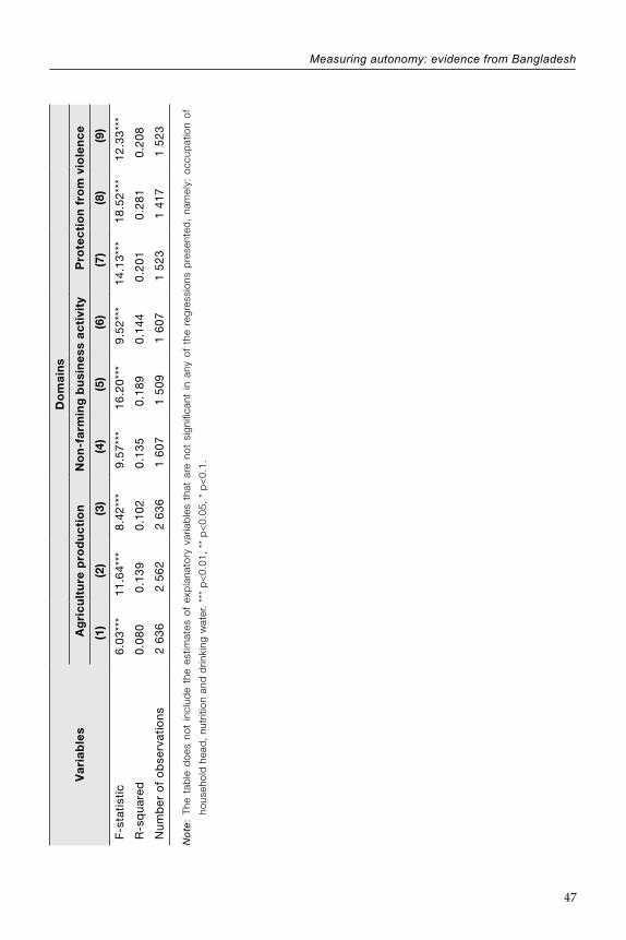
Measuring autonomy: evidence from Bangladesh
47
Do
ma
ins
Va
ria
ble
sA
gri
cu
ltu
re p
rod
uc
tio
nN
on
-fa
rmin
g b
usi
ne
ss a
cti
vity
Pro
tec
tio
n f
rom
vio
len
ce
(1)
(2)
(3)
(4)
(5)
(6)
(7)
(8)
(9)
F-s
tati
stic
6.0
3**
*1
1.6
4**
*8
.42
***
9.5
7**
*1
6.2
0**
*9
.52
***
14
.13
***
18
.52
***
12
.33
***
R-s
qu
ared
0.0
80
0.1
39
0.1
02
0.1
35
0.1
89
0.1
44
0.2
01
0.2
81
0.2
08
Nu
mb
er o
f o
bse
rvat
ion
s2
63
62
56
22
63
61
60
71
50
91
60
71
52
31
41
71
52
3
No
te:
The
tab
le d
oes
not
incl
ude
the
estim
ates
of
exp
lana
tory
var
iab
les
that
are
not
sig
nific
ant
in a
ny o
f th
e re
gres
sion
s p
rese
nted
, na
mel
y: o
ccup
atio
n of
hous
ehol
d h
ead
, nu
triti
on a
nd d
rinki
ng w
ater
. **
* p
<0.
01,
** p
<0.
05,
* p
<0.
1.
Asia-Pacific Sustainable Development Journal Vol. 25, No. 2
48
Tables 6.1 (sample of men) and 6.2 (sample of women) present the estimates of equation (2) for the RAI in the same domains considered above, except “livestock raising”. For each domain-specific RAI we present three sets of results, where we examine sensitivity of adding the following explanatory variables:
(i) The domain-specific indicator “feel can make decision”;
(ii) The domain-specific indicators “feel can make decisions” and “satisfaction with decisions made”; and
(iii) The domain-specific indicator “feel can make decisions” and the general indicator “power to make important decisions”.
The indicator “feel can make a decision” is only significantly associated with the RAI in some domains. So, as suggested by the correlation analysis, this indicator is not a good candidate to proxy autonomy.
On the other hand, the indicators “satisfaction with decisions made” and “power to make important decisions” are significantly associated with higher levels of autonomy of men and women in all domains. Nevertheless, they still do not account for a large portion of the variation, which is indicated by the low magnitude of the R-squared and the fact that in most cases their inclusion as explanatory variables does not affect the significance of the other determinants of autonomy (except for the variable “feel can make the decisions”). Under these circumstances, it remains unclear whether these indicators can be used as proxies for autonomy, or whether they are simply indicators that are also correlated with autonomy.

Measuring autonomy: evidence from Bangladesh
49
VI. CONCLUSION
This paper provides a detailed examination of the Relative Autonomy Index (RAI), using data representative of Bangladeshi rural areas. We report mixed, but largely positive, results in terms of the conceptual validity of the RAI. We find evidence of three dimensions in the data, each corresponding to one of the motivation subscales, exactly as predicted by the measurement model. The surprise is that we do not always find an ordered correlation among the three motivation subscales as expected by the self-determination continuum. Instead, we find gender patterns of correlations. In the sample of men, we find that external and introjected motivations are strongly correlated, whereas both are weakly correlated with autonomous motivations, as predicted by the RAI measurement model. In the sample of women, we find that external motivation is positively and strongly correlated with introjected and autonomous motivations, yet the correlations between introjected and autonomous motivations tend to be weak. We speculate that the strong correlation between external and autonomous motivation arises because Bangladeshi women internalize societal norms and “make them their own”; but more qualitative work is needed to study this issue.
Our exploratory analysis of the determinants of men’s and women’s autonomy in Bangladesh shows that neither age, education nor income are suitable proxies for autonomy. We also find no robust evidence that other indicators on decision-making adequately proxy autonomy.
The search for rigorous, transparent and domain-specific measures of empowerment that can be used for gender analysis remains ongoing. Many indicators have failed to fulfil the criteria required for rigorous quantitative analyses of women’s empowerment. This paper demonstrates that the RAI as implemented in Bangladesh is a reliable indicator of autonomy, and adds value and information to variables such as education, expenditure, age, mobility or decision-making. It distinguishes male from female autonomy, and differentiates autonomy levels across different domains. As such, the RAI very much remains a strong candidate for empirical studies of empowerment. To further advance this field, it is necessary to explore qualitatively what appear to be cultural influences on women’s external motivation in Bangladesh, implement the RAI in additional geographic and cultural settings and explore its validity and reliability in those settings.

Asia-Pacific Sustainable Development Journal Vol. 25, No. 2
50
REFERENCES
Abell, N., D. W. Springer, and A. Kamata (2009). Developing and Validating Rapid Assessment Instruments. New York: Oxford University Press.
Ahmed, A. (2013). Bangladesh Integrated Household Survey (BIHS) 2011-2012. Washington, D.C.: International Food Policy Research Institute (datasets). Available from http://hdl.handle.net/1902.1/21266.
Alkire, S. (2005). Subjective quantitative studies of human agency. Social Indicators Research, vol. 74, No. 1, pp. 217-260.
Alkire, S. (2008). Concepts and measures of agency. Oxford Poverty and Human Development Initiative (OPHI) Working Paper, No. 9. Oxford, United Kingdom: OPHI. Available from https://ophi.org.uk/working-paper-number-09/.
Alkire, S., and others (2013). The women’s empowerment in agriculture index. World Development, vol. 52, pp. 71–91.
Allen, E., and C. Seaman (2007). Likert scales and data analyses. Quality Progress, vol. 40, No. 7 pp. 64-65.
Alsop, R., M. F. Bertelsen, and J. Holland (2006). Empowerment in Practice: From Analysis to Implementation. Washington, D.C.: World Bank. Available from http://commonweb.unifr.ch/artsdean/pub/gestens/f/as/files/4760/24995_105259.pdf.
Becker, E. (2012). Themes from feed the future women’s empowerment in agriculture index: report from qualitative case studies in Bangladesh, Guatemala and Uganda. Unpublished report submitted to the International Food Policy Research Institute. Washington, D.C.
Brown, J. (2011). Likert items and scales of measurement? Shiken: JALT Testing & Evaluation SIG Newsletter, vol. 15, No. 1, pp. 10-14.
Carifio, J., and R. Perla (2007). Ten common misunderstandings, misconceptions, persistent myths and urban legends about likert scales and likert response formats and their antidotes. Journal of Social Sciences, vol. 3, No. 3, pp. 106-116.
Chirkov, V. I. (2009). A cross-cultural analysis of autonomy in education: A self-determination theory perspective. Theory and Research in Education, vol. 7, No. 2, pp. 253-262.
Chirkov, V. I., R. M. Ryan, and K. M. Sheldon (2011). Human Autonomy in Cross-cultural Contexts: Perspectives on the Psychology of Agency, Freedom, and Well-being. Dordrecht, Nederlands: Springer.
Chirkov, V. I., and others (2003). Differentiating autonomy from individualism and independence: a self-determination theory perspective on internalization of cultural orientations and well-being. Journal of Personality and Social Psychology, vol. 84, No. 1, pp. 97-110.
Cortina, J. M. (1993). What is coefficient alpha? An examination of theory and applications. Journal of Applied Psychology, vol. 78, No. 1, pp. 98-104.
Deci, E. L., and R. M. Ryan (2012). Motivation, personality, and development within embedded social contexts: an overview of self-determination theory. In Oxford Handbook of Human Motivation, R. M. Ryan, ed. Oxford, United Kingdom: Oxford University Press.
Drèze, J., and A. Sen (2013). An Uncertain Glory: India and its Contradictions. Princeton: Princeton University Press.
Guio, A. C., D. Gordon, and E. Marlier (2012). Measuring material deprivation in the EU: indicators for the whole population and child-specific indicators. Eurostat Methodologies and Working

Measuring autonomy: evidence from Bangladesh
51
Paper. Luxembourg: Publications office of the European Union. Available from: http://epp.eurostat.ec.europa.eu/cache/ITY_OFFPUB/KS-RA-12-018/EN/KS-RA-12-018-EN.PDF.
Hemker, B. T., K. Sijtsma, and I. W. Molenaar (1995). Selection of unidimensional scales from a multidimensional item bank in the polytomous Mokken IRT model. Applied Psychological Measurement, vol. 19, No. 4, pp. 337-352.
Ibrahim, S., and S. Alkire (2007). Agency and empowerment: a proposal for internationally comparable indicator. Oxford Development Studies, vol. 35, No. 4, pp. 405-430.
Kishor, S., and L. Subaiya (2008). Understanding Women’s Empowerment: A Comparative Analysis of Demographic and Health Surveys (DHS) Data. DHS Comparative Reports 20. Calverton, United Kingdom: Macro International.
Levesque, C. S., and others (2007). Validating the theoretical structure of the treatment self-regulation questionnaire (TSRQ) across three different health behaviours. Health Education Research, vol. 22, No. 5, pp. 691–702.
Malhotra, A., S. Schuler, and C. Boender (2002). Measuring women’s empowerment as a variable in international development. Background paper prepared for the World Bank Workshop on Poverty and Gender: New Perspectives. 28 June. World Bank. Available from http://siteresources.worldbank.org/INTGENDER/Resources/MalhotraSchulerBoender.pdf.
Narayan, D. (2005). Conceptual framework and methodological challenges. In Measuring Empowerment: Cross Disciplinary Perspectives, D. Narayan, ed. Washington, D.C.: World Bank. Available from https://openknowledge.worldbank.org/handle/10986/7441.
Panda, P., and B. Agarwal (2005). Marital violence, human development and women’s property status in India. World Development, vol. 33, No. 5, pp. 823–850.
Ryan, R. M., and J. P. Connell (1989). Perceived locus of causality and internalization: examining reasons for acting in two domains. Journal of Personality and Social Psychology, vol. 57, No. 5, pp. 749-761.
Ryan, R. M., and E. L. Deci (2000). Self-determination theory and the facilitation of intrinsic motivation, social development, and well-being. American Psychologist, vol. 55, No. 1, pp. 68-78.
Samman, E., and M. E. Santos (2009). Agency and empowerment: a review of concepts, indicators and empirical evidence. Oxford Poverty and Human Development Initiative (OPHI) Working Paper, No. 10a. Oxford, United Kingdom: OPHI. Available from https://ophi.org.uk/ophi-research-paper-10a/.
Sraboni, E., A. R. Quisumbing, and A. U. Ahmed (2013). The Women’s Empowerment in Agriculture Index: Results from the 2011-2012 Bangladesh Integrated Household Survey. Project report submitted to the United States Agency for International Development. Dhaka: International Food Policy Research Institute. Available from http://ebrary.ifpri.org/cdm/ref/collection/p15738coll2/id/127504.
Sraboni, E., and others (2013). Women’s empowerment in agriculture: What role for food security in Bangladesh? World Development, vol. 61, pp. 11-52.
StataCorp (2013). Stata Statistical Software: Release 13. College Station, Texas: StataCorp LP.
Vaz, A., P. Pratley, and S. Alkire (2016). Measuring women's autonomy in Chad using the Relative Autonomy Index. Feminist Economics, vol. 22, No. 1, pp. 264-294.


53
FACTORS INFLUENCING MATERNAL HEALTH CARE IN NEPAL: THE ROLE OF SOCIOECONOMIC INTERACTION
Sharmistha Self and Richard Grabowski*
This paper relies on an extensive data set on Nepalese families to examine factors influencing the extent to which maternal health care is provided. A number of hypotheses are examined: Do social networks that evolve to support market exchange allow for the dissemination of knowledge concerning the effectiveness of maternal care? Do social norms regarding maternal care have a significant influence on decisions to seek such care? Do educational spillover effects play an important role in decision-making concerning maternal health care? Does gender preference influence the extent to which a family supports health care for expectant mothers? Finally, are women who are perceived as more independent likely to choose additional care?
JEL classification: O10, O53, I10
Keywords: Nepal, maternal health, socioeconomic factors
I. INTRODUCTION
The availability of maternal health care continues to be a major problem in developing countries. There were an estimated 303,000 maternal deaths worldwide in 2015, with 99 per cent of those deaths in developing countries. About two-thirds of maternal deaths occurred in sub-Saharan Africa with one-fifth in South Asia. Many of these deaths could have been prevented had maternal health care been available: “Women are not dying during pregnancy and childbirth from complicated conditions that are hard to manage. Women are dying because they do not receive the health care they need” (Lewis, 2008, p. 2). Reducing maternal mortality and improving maternal health has become a global health priority, demonstrated by its inclusion in the United Nations Millennium Development Goals (MDGs) and the Sustainable Development Goals (SDGs). It is widely recognized that reducing maternal mortality
* Sharmistha Self, Department of Economics at University of Northern Iowa (email: [email protected]). Richard Grabowski, Professor of the Department of Economics at the Southern Illinois University(email: [email protected] ).

Asia-Pacific Sustainable Development Journal Vol. 25, No. 2
54
is dependent upon the provision of maternal health services, both prenatal and postnatal, by trained medical personnel (Adhikari, 2016). However, the provision of such services is not enough. Policy must also be aimed at reducing gender bias so that women can make effective use of the maternal health services actually provided.
The present study focuses on Nepal – a relatively small developing country in South Asia. The social system in Nepal exemplifies the patriarchal social system commonly found in many South Asian countries. Gender differences and inequalities are present in several distinct socioeconomic areas within the Nepalese community. However, despite its social system and underlying gender inequalities, Nepal has achieved a significant reduction in maternal mortality over the past 25 years. In 1990, there were 901 deaths per 100,000 live births; by 2015, this rate had been reduced to 258 per 100,000 live births. While this reduction appears to be a significant achievement, the maternal mortality rate is nonetheless much higher than other South Asian countries (Adhikari, 2016). Many ascribe the reduction in maternal mortality to the Safe Motherhood Programme initiated by the government of Nepal, in collaboration with the World Health Organization (WHO). This programme was founded with three objectives: (1) providing round-the-clock emergency obstetric care; (2) ensuring the presence of skilled attendants at births; (3) promoting public awareness of safe motherhood practices.
Some scholars have questioned the validity of maternal mortality estimates generated from the data in the Nepal Demographic and Health Survey. Their scepticism is partly due to the lack of clarity over what changes could have accounted for the significant drop in maternal mortality rate. The moderate improvements in key services appear insufficient to explain the dramatic drop in maternal deaths. Moreover, during much of the relevant period, Nepal had been involved in a prolonged internal armed conflict, which would have likely disrupted many of the government programmes and services. As such, it was not at all clear whether government programmes alone could have brought about such a significant drop in maternal mortality, nor is it even clear that the programmes had achieved their full potential. Finally, estimates of maternal mortality rates in data from smaller regions in Nepal were much higher (Prize and Bohara, 2013).
Notwithstanding whether there has been, in fact, a significant improvement in maternal mortality rates, inadequate maternal care remains a significant problem in Nepal. As such, this paper chooses not to focus on maternal mortality, but rather on maternal care and the link between inadequate maternal care and maternal mortality rates. Specifically, it analyses factors that influence women’s use of maternal care services in Nepal. Evidence indicates that a majority of maternal and infant deaths arising out of pregnancy complications could have been averted with early and frequent prenatal check-ups (Kamal, 2009; Reynolds, Wong and Tucker, 2006). In addition, according to the World Health Organization (2010), maternal and neonatal

Factors influencing maternal health care in Nepal: the role of socioeconomic interaction
55
problems could be reduced if women were able to receive more appropriate and timely postnatal care. Inadequate maternal care in Nepal not only compromises the welfare of women, but also poses a significant obstacle to long-term growth and development in Nepal. Part of the problem is lack of facilities, requiring women to travel long distances to receive care. However, another part of the problem is the number of obstacles preventing women from accessing services even when they are available. This paper will examine a range of factors that influence maternal care in Nepal, based on household survey data from the 2010 – 2011 Nepal Living Standard Survey III.
The literature on this issue is extensive (Glei, Goldman and Rodriguez, 2003; Bloom, Wypij and Das Gupta, 2001; Chakrabarti and Chaudhuri 2007; Das Gupta and others, 2003; Karkee, Lee and Binns, 2013), and for the most part, this paper relies on variables cited in previous studies. However, five additional variables representing five new hypotheses have been introduced into the analysis of this paper.
The first variable or hypothesis concerns the importance of social networks in facilitating information exchange on health-care related issues. A study by Deri (2005) draws attention to the association between social networks and health care utilization. However, relatively little has been done to look specifically at the role of social networking or social interactions on health-care decisions by pregnant women before and after childbirth. Mukong and Burns (2015) have found that social networks have a beneficial impact on maternal health care utilization behaviour, enhancing prenatal completion and the probability of early prenatal check-ups among pregnant women in Tanzania. Social networks that allow for and support market exchange may also act as a mechanism for conveying information concerning health care, including maternal health care. As a place where people congregate regularly, markets offer a platform for buyers to interact with a multiplicity of sellers and with each other. It is hypothesized that in the course of regular meaningful conversations, social connections develop within these markets, with a likelihood of knowledge spillover into other topics, including information relating to maternal health care. Therefore, people engaging regularly in market activities will likely have access to information about maternal care services available in their region, and thus may be more likely to participate in prenatal and postnatal care visits with trained professionals. In this respect market activity, specifically participation, and buying and selling in markets could generate greater knowledge-sharing relating to health.
The second variable or hypothesis posited in this paper suggests that when a woman lives in an area where the average level of education is relatively high, she is more likely to be exposed to information about maternal care and its effectiveness through neighbours and peers. This exposure to knowledge will likely increase the probability that whatever a woman’s educational level, she will pursue maternal care.

Asia-Pacific Sustainable Development Journal Vol. 25, No. 2
56
The third variable or hypothesis posited in this paper considers the extent to which accessing maternal health care has become a social norm in the region. Social norms appear to play an important role in determining health-care decisions. This type of social norm can be a powerful influence on decision-making.
The fourth variable or hypothesis posited in this paper focuses on the extent to which women are able to make decisions independently. Over and above the role of social interactions via markets, educational spillovers and social norms, this paper looks at the impact of other socioeconomic factors on maternal health care utilization. Empirical evidence has suggested that a variety of household and community factors influence maternal health services in both developing and developed countries (Gage, 2007; Kamal, 2009; Jat, Ng, and San Sebastian, 2011). For instance, in many regions in Asia, especially South Asia, the presence of a patriarchal social system (ADB, 1999) means that men will generally make the important decisions with respect to financial matters, major household economic decisions and health matters. Within the context of this type of social structure, especially in rural areas, one would indeed expect that households in which females lack autonomy are likely to spend less on maternal health care. Thus, the more autonomous a woman, the more likely expenditure will be made on maternal health care.
The fifth variable or hypothesis posited in this paper concerns the measure of son bias - much of South Asia is characterized by preference for a son or male heirs. Most families prefer sons for a variety of cultural and social reasons which have evolved over time (Priya and others, 2012). These norms and cultural values are likely to influence expenditure on maternal health care. Specifically, if the family already has a son, it may affect expenditure on prenatal and postnatal care in subsequent pregnancies. Thus, if a son preference has already been satisfied, it is suggested that less prenatal and postnatal care will be provided for additional pregnancies.
The remainder of the paper will be structured as follows. Under section II, the methodology will be explained in detail and general characteristics of the data set will be presented. Section III will analyse empirical results. Section IV will provide a summary of the paper with policy implications explored.
II. DATA AND EMPIRICAL MODEL
The empirical estimation utilized an ordered logit estimation, which is a direct generalization of the ordinary two-outcome logit model. Ordered logit models are used to estimate relationships between an ordinal-dependent variable and another set of independent variables. Under the ordered logit model, the actual values taken by the dependent variable are irrelevant, except that larger values are assumed to

Factors influencing maternal health care in Nepal: the role of socioeconomic interaction
57
correspond to “higher” outcomes. With reference to the analysis, higher outcomes indicate greater usage of maternal care by the mother. The dependent ordinal variable ranges in value from zero to two, where zero represents a woman not receiving any type of maternal care; one represents a woman receiving at least one form of care - prenatal or postnatal; two represents a woman receiving both prenatal and postnatal care. It is assumed that two is the desirable outcome, while zero is the least desirable outcome. In ordered logit, an underlying score is estimated as a linear function of the independent variables and a set of cut-points. The probability of observing outcome (i) corresponds to the probability that the estimated linear function, plus random error, is within the range of the cut-points estimated for the outcome:
Pr (outcomej = i) = Pr (ki-1 < β1x1j + β2x2j + _ _ _ + βkxkj + uj ≤ ki),
where uj is assumed to be logistically distributed in ordered logit and k represents the number of outcomes, which in this case is three.
The empirical model to be estimated will take the form:
Maternal_careijk = a0 + a1Indivijk + a2HHijk + a3Communityijk + eij (1)
where Maternal_care measures the extent of maternal care that a woman i, living in household j and community k receives. Indivijk, HHijk, and Communityijk represent individual, household and community specific characteristics of the woman and her spouse.
The selection of explanatory variables is influenced, as discussed above, by existing literature, theory and hypotheses being tested in this paper. It is hypothesized that the extent of maternal care that a woman receives is dependent on individual, social and economic factors. For ease of analysis these characteristics are bundled under individual, household and community-level characteristics. Individual characteristics can be economic and/or social in nature, as are household characteristics. Community characteristics measure how individual behaviour is influenced by the social spillover of community-level behaviour. In addition, we have controlled for regional characteristics. The definitions of all the variables used are provided in table 1.

Asia-Pacific Sustainable Development Journal Vol. 25, No. 2
58
Table 1. Definition of variables
Maternal_care Variable taking value 0 if woman received no maternal care; 1 if she received either prenatal or postnatal care; and 2 if she received both prenatal and postnatal care
Age Age of respondent
Age_sq Age squared
Edu Education of respondent (categorical variable)
Head_Edu Education of husband/household head (categorical variable)
WageWork Dummy variable taking value 1 if respondent works for wages and 0 otherwise
Good_health Dummy variable taking value 1 if respondent is neither disabled nor suffers from any chronic illness or missed any days of work or regular activities due to illness
Time_to_healthcare Time (in minutes) to nearest health-care facility
Health_autonomy Dummy variable taking value of 0 if someone else made the decision about a woman seeking health care; 1 if the spouse alone made the decision; 2 if the decision was a joint one between the woman and her spouse; and 3 if the woman alone made this decision
Birth_order Birth order of last child
Shoptime Time spent (in minutes) by household members in the market shopping for the family
HH_Size Number of people living in the house
Sons Number of sons
High_Caste Dummy variable taking value 1 if family belongs to high caste of Brahman, Newar or Chetri and 0 otherwise
Landowner Dummy variable which takes value 1 if the household owns land and 0 otherwise
Home_electric Dummy variable which takes value 1 if household has electricity and 0 otherwise
Community_Edu Average education level of members of the primary sample units where the respondent lives
Community_maternalcare Proportion of women in the primary sample units (where the respondent lives) that received both prenatal and postnatal care
Urban Dummy variable that takes value 1 if the respondent lives in an urban region and 0 otherwise
Individual level explanatory variables relate to the woman and her husband. In terms of individual variables relating to the woman, we first controlled for age (Age). This was a continuous variable, commonly included in empirical analysis on maternal care. We also included a quadratic term which is the square of the woman’s age

Factors influencing maternal health care in Nepal: the role of socioeconomic interaction
59
(Age_sq) to see whether the relationship between age and extent of maternal care was non-linear. We then carried out estimations relating to the age variable, constructing dummy variables to represent different age groups. One might expect that older women would be less likely to utilize maternal health care as they would be more influenced by tradition. However, older women may also have accumulated much more information concerning maternal care through experience. Thus, it is unclear whether older women will be less or more likely to involve themselves in maternal care.
We also included information concerning the woman’s employment status as an explanatory variable (WageWork). This was a binary variable: one represented a woman who worked and received wages, and zero represented a woman who did not receive wages for work. The assumption was that if a woman worked for wages then she could potentially contribute towards the finances of the family. This was expected to increase her bargaining power within the family, while at the same time increasing her access to resources. The importance of a woman’s ability to contribute financially towards household expenses is supported by empirical research on female autonomy. This literature also mentions the presence of a son or sons (Sons) as one another avenue in which a woman’s autonomy may be enhanced within a household in a patriarchal society (Jejeebhoy and Sathar, 2001). That said, the impact of having a son or sons on a woman’s utilization of maternal care is not straightforward. Although having a son or sons may enhance women’s bargaining power within the household, son preference behaviour may nonetheless affect and limit how resources are allocated to maternal care, especially if the family has already had one or more sons. Thus, if the net impact of having sons is positive, it would imply that the positive impact of increased female autonomy outweighs the negative impact of son preference behaviour and vice versa. This is one of the five new variables and hypotheses introduced into the analysis in this paper.
The education level of the woman (Edu) and her spouse/household head (Head_Edu) are included as additional explanatory variables. Education level is segregated into a categorical variable ranging from zero to four in value. A value of zero signifies being illiterate; a value of one signifies being literate; a value of two signifies primary-level education (grades 1 to 5); a value of three signifies secondary-level education (grades 6 to 12); and a value of four signifies tertiary education (education above secondary-level education). We also carried out alternative estimations where we included education as separate dummy variables to represent the categories explained above, however these results are not represented here. These categorical variables are expected to have a positive impact on maternal care. Education has frequently been utilized as an indicator of a mother seeking maternal care. Several studies have shown that women with better education were more likely to receive the recommended number
Asia-Pacific Sustainable Development Journal Vol. 25, No. 2
60
of prenatal care visits (Nielsen and others, 2001; Erci, 2003). Moreover, educated women have been shown to be more likely to start prenatal care visits earlier than less educated women (Miles-Doan and Brewster, 1998; Matthews and others, 2001). Several studies have also examined the importance of a husband’s education in terms of a woman receiving maternal care. For example, in the State of Andrea Pradesh in India, a husband’s education was a statistically significant predictor, though in the State of Karnataka, this was not the case (Navaneetham and Dharmalingam, 2002).
We did not have information on the cost of utilizing maternal care. In the absence of a direct measure of cost, we employed an indirect measure – the time required to travel to the nearest health-care facility (Time_to_healthcare). It was assumed that the farther away a person lived from a health-care facility the less likely they would be to utilize such services. On this basis, the length of time required to access care was considered as a cost of care. One would expect this variable to have a negative impact on likely use of maternal care. This type of variable was also relied upon in Glei, Goldman and Rodriguez (2003) and Magadi, Madise and Rodrigues (2000) as a predictor of women receiving maternal care.
We further included two additional individual level variables that relate to health of the woman. The first relates to the condition of her health, while the second relates to her freedom or autonomy to seek her own health care. We did this in order to investigate whether being disabled, chronically ill or missing work due to illness had an impact on the extent of maternal care that a woman was able to receive. Given that most people in the sample lived in rural areas with low levels of education, one might expect that being healthy could reduce the likelihood of a woman receiving greater maternal care from a health practitioner. The health status variable (Good_health) is a binary variable which took a value of one if the woman was disabled or chronically ill or she had been sufficiently ill in the past year to have not been able to carry out her regular duties, or zero if she has not had any medical issues.
The method by which we measured a woman’s autonomy (Health_autonomy) to seek health care requires some explanation. First, women were asked whether a decision was made regarding their health care and who was involved in this decision-making. There are four possible responses: a woman made the decision on her own; she made it jointly with her spouse; her spouse alone made the decision; someone else made the decision. We created a categorical variable using this information. The variable took the value of zero if someone else made the decision; it took the value of one if the spouse alone made the decision; it took the value of two if the decision was made jointly between the woman and her spouse; it took the value of three if the woman alone made this decision. Khanal and others (2014) use a similar set of autonomy variables to analyse a mother’s usage of postnatal care in Nepal. It is anticipated that the greater the autonomy a woman enjoyed in terms of seeking

Factors influencing maternal health care in Nepal: the role of socioeconomic interaction
61
her own health care, the more likely she would be to receive and utilize such care. This is the second new variable and hypothesis incorporated into the paper.
Finally, we included the birth order of the last child (the most recent birth for whom the respondent is answering the questions relating to maternal care). This variable (Birth_order) is expected to have a negative impact on receiving maternal care since the more children a woman has, the greater the financial stress on her family to provide for maternal care.
Next, we turn our attention to the household-level explanatory variables. Of particular interest is the measure of social spillover effects from market place interactions. In order to capture this impact, we construct a variable (Shoptime), which calculates the amount of time that household members spend in the market for the purpose of household shopping. This variable measures the time spent in the market directly buying and selling for the needs of the household. It is therefore a fairly narrow definition of market activity, but it is the only measure provided in the data set. It is anticipated that more time spent in the market will translate into better maternal care via knowledge-sharing taking place through social interactions. This is the third new variable and hypothesis incorporated into the analysis of this paper.
In addition to the above, we controlled for caste as a measure of social status of the household. We decided not to control for religion because nearly 100 per cent of the people in our sample self-identified as Hindu. The High_Caste variable is a binary variable: the value of one represents the respondent belonging to a high caste, and the value of zero represents the respondent belonging to a low caste. Alternatively, we constructed another binary variable which attributes the value of one to a Dalit household, and the value of zero to all other households. Results relating to Dalit households are not presented here. Given that Nepal is a caste-based society, caste is expected to play a role in determining social status. Jejeebhoy and Sathar (2001) find that female autonomy is influenced by social status along with education and economic activity. Thus, caste is expected to play a role in determining a woman’s autonomy, which in turn is expected to influence the allocation of resources towards her maternal care.
Other household level social characteristics considered were the number of members in the household (HH_Size), whether or not the household owns land (Landowner) and whether or not the household has access to electricity (Home_electric). HH_Size is a continuous variable measuring the number of members in a household. We were interested in family size to ascertain whether the number of people in a family affects the probability of a woman receiving maternal care. One might argue that this could have either a positive or a negative impact. The positive impact would have likely come from more family members being concerned for the woman’s welfare, while

Asia-Pacific Sustainable Development Journal Vol. 25, No. 2
62
the negative impact may come from the economic pressure of taking care of a large family, which might reduce allocation of resources for the woman. The net impact therefore remains unclear at this time.
The variable Landowner is a dummy variable which takes value of one if the household owns land and zero otherwise. Anecdotal evidence suggests that land ownership is seen as an economic status symbol of sorts in Nepal. This is supported by the fact that over 76 per cent of households in our sample own some land. While being a landowner may depict economic status (which would have a positive impact), it also reflects a more traditional household (which may have a negative impact). The net impact of this variable is therefore unclear.
The variable Home_electric takes the value of one if a home is electrified and zero if the home does not have electricity. This variable is assumed to be a proxy reflecting the extent of economic development in the area where the respondent lives, and thus would likely have a positive impact on maternal care. Another alternative measure of economic status is household income, but we do not include this variable due to its high collinearity with the variable measuring women’s work status (discussed earlier).
We also include two community-level variables where we expect some social spillover effects via social interactions will influence the degree of maternal care that a woman receives. Since we do not have village-specific data, we rely on the primary sampling units to represent communities. We include the average level of education in the primary sampling units where the woman lives (Community_Edu). We also consider the proportion of women in the primary sampling units who received both prenatal and postnatal care (Community_maternalcare). Literature provides evidence that individuals whose neighbourhoods are healthier are more likely to experience better health outcomes and lower exposure to disease (Ludwig, Duncan, and Hirsch, 2001; Katz, Kling and Liebman, 2001). However, while both of these variables are expected to have a positive impact on the dependent variable through their positive externality effect, we are not including them simultaneously in order to avoid multicollinearity issues. These represent the fourth and fifth new variables and hypotheses introduced into this paper. In addition to the individual, household and community influences, we also controlled for regional influences by controlling for urban region (Urban) versus rural regions. The Urban variable is a dummy variable that takes a value of one if a woman lives in an urban area and zero if a woman does not live in an urban area. It is assumed that women living in urban areas will have less difficulty accessing maternal care.
The paper utilizes household survey data from the Nepal Living Survey Third Round carried out by the Census Bureau of Nepal in 2010-2011, in conjunction with the World

Factors influencing maternal health care in Nepal: the role of socioeconomic interaction
63
Bank. The surveys followed the Living Standards Measurement Survey methodology developed and promoted by the World Bank. Randomly selected households were clustered within primary sampling units (PSU), which were either individual wards, sub-wards or groups of contiguous wards in the same village development council. Since we do not have specific village information, we relied on the PSUs in lieu of villages, utilizing some PSU-specific information to control for regional heterogeneity. Table 2 provides summary statistics of the variables.
Table 2. Summary statistics
Variables Obs. Mean Std. Dev. Min Max
Age 1 633 26.39988 6.076609 14 51
Edu 1 633 1.83711 0.9250964 0 4
Head_Edu 1 633 1.812002 0.922647 0 4
Sons 1 633 1.28414 1.056655 0 6
HH_Size 1 633 6.512554 2.919676 2 20
High_Caste 1 633 0.3392529 0.4736008 0 1
Landowner 1 633 0.76485 0.4242225 0 1
Home_electric 1 633 0.6576852 0.4746297 0 1
WageWork 1 633 0.0385793 0.1926491 0 1
Time_to_healthcare 1 633 66.58216 71.99192 0 520
Good_health 1 633 0.9007961 0.2990272 0 1
Community_Edu 1 633 1.400115 0.2524175 1 2.508197
Shoptime 1 633 0.3093819 0.5548772 0 4.285714
Health_autonomy 1 633 1.401715 1.11597 0 3
Urban 1 633 0.2455603 0.4305508 0 1
Community_maternalcare 1 633 0.2094305 0.2669591 0 1
Birth_order 1 631 3.044145 1.83203 1 11
Our dependent variable is maternal care utilization. Most papers that analyse maternal care utilization focus either on prenatal or postnatal care. This paper took a more holistic approach to maternal care, incorporating both prenatal and postnatal care. The survey addressed its questions on maternal-related care to all women who had given birth in the three years prior to the survey. A group of 1,633 women forms the sample for the empirical analysis.

Asia-Pacific Sustainable Development Journal Vol. 25, No. 2
64
III. EMPIRICAL ANALYSIS
We use ordered logit to carry out our estimations, since the dependent variable is an ordinal variable, ranging in value from zero to two, with two representing a woman who received both prenatal and postnatal care. Thus, the higher the value of the dependent variable, the greater the likelihood that the woman received higher-quality maternal care. Needless to say, we are making an implicit assumption that receiving prenatal and postnatal care from a trained doctor/practitioner is preferable to not receiving such care.
Explanatory variables are added to the base model in various combinations in order to verify the sensitivity of results to the inclusion of different variables, as well as to determine the robustness of the results, which remain very consistent. We control for issues such as multicollinearity by not including highly correlated variables simultaneously in any estimation. For example, we do not include Community_Edu and Community_maternalcare in the same estimation. In addition, earning wages from work (WageWork) and health autonomy (Health_autonomy) are not included in the same estimation, since there is likely to be a high correlation between the two. These are the reasons that six different versions of the model are estimated. It allows one to determine whether the results are robust using different formulations of the model.
Findings of the study
Table 3 represents ordered logit results, and presents six different specifications of equation (1). Our analysis initially focused on the five new variables utilized in the paper. Under the first hypothesis, it was argued that households more involved in market exchange would be more likely to receive information concerning maternal care and thus more likely to make use of these services. Indeed, the results indicated that those families spending more time shopping (Shoptime) were associated with a greater use of maternal care – this held for all estimations. Thus, social networks that evolved in market exchange situations seemed to encourage the spread of information concerning the usefulness of maternal health care, leading to women indeed receiving increased amounts of such care.
Under the second hypothesis, it was suggested that in those areas where the proportion of women utilizing maternal health care was high (Community_maternalcare), the use of maternal health care by individual women would also be high. That is, if there was a social norm attached to using maternal care, then individuals would be more likely to use these services. Indeed, this variable was positive and significant in all relevant estimations. Thus, a social norm validating the use of maternal health care did seem to promote the use of such care.
The third hypothesis postulated that the higher the average level of education in any particular area (Community_Edu), the more likely that there would be a spillover effect favouring the use of maternal care. Indeed, this appeared to be the case for

Factors influencing maternal health care in Nepal: the role of socioeconomic interaction
65
all relevant estimations. These results pointed to the importance of social spillover effects in improving maternal care utilization by women in Nepal. Similar conclusions were reached by Mukong and Burns, (2015) and Gage (2007) in developing countries of Africa.
Under the fourth hypothesis, increased female autonomy was thought to lead to increased maternal care. Female autonomy was measured by the variables Health_autonomy and WageWork. The signs for these two variables were both positive and significant for all relevant estimations. Thus, a woman who had some input regarding health-care decisions was more likely to receive maternal care. In addition, if the woman earned a wage, it also seemed to enhance her autonomy leading to an increase in the use of maternal health-care services. The results relating to the woman’s autonomy over her health care, and the positive impact emanating from her ability to work for wages were similar to those found in Khanal and others (2014). Pallikadavath, Foss, and Stones (2004) also found that a woman’s autonomy was linked with receiving prenatal care in rural north India. In addition, Erci (2003) found a woman’s employment outside the home had a significant impact on her receiving prenatal care.
Finally, the fifth hypothesis examined the role of gender-bias. In other words, did already having a son or sons result in less maternal care for the mother? The sign on the Sons variable was statistically significant and negative. It implied that once a son was born into a family, and son preference was fulfilled, it was likely that a woman would receive less maternal health care for additional pregnancies.
Results for other variables at the individual level were also interesting. From the results presented in table 3, one can see that education played an important role in maternal care utilization. The education of a woman (Edu) and her husband (Head_Edu) had both a positive and statistically significant impact on maternal care, although the size of the coefficient for women’s education was greater. The quadratic age variable (Age_sq) was found to be negative and statistically significant, implying that as women grew older, they were much less likely to receive maternal care. The results also showed that a woman’s current health (Good_health) was associated with a lower probability of maternal care use. In other words, the better the health of an expectant mother, the less likely it would be that she would receive maternal care during or after her pregnancy. The results relating to health seemed to reflect those of Chowdhury, Mahbub and Chowdhury (2003) which found that prenatal care was not seen as essential unless there was physical discomfort during pregnancy and complications in previous pregnancies or childbirth. Finally, as one would expect, the results showed that the greater time it took to access a health-care facility (Time_to_healthcare), the lower the probability that women would access maternal care services. Several qualitative studies have shown that distance to services or barriers to accessing services played a role in the utilization of prenatal care services (Griffith and Stephenson, 2001; Chowdhury, Mahbub, and Chowdhury, 2003; Myer and Harrison, 2003; Mathole and others, 2004).

Asia-Pacific Sustainable Development Journal Vol. 25, No. 2
66
Ta
ble
3.
Ord
ered
log
it e
stim
atio
ns
of
the
det
erm
inan
ts o
f m
ater
nal
hea
lth
car
e
Va
ria
ble
s(1
)(2
)(3
)(4
)(5
)(6
)
Ag
e0
.18
8**
*0
.08
94
0.0
39
00
.06
55
0.1
50
**0
.03
90
(0.0
63
1)
(0.0
67
7)
(0.0
69
6)
(0.0
68
8)
(0.0
64
3)
(0.0
69
6)
Ag
e_sq
-0.0
03
96
***
-0.0
02
42
**-0
.00
13
3-0
.00
17
5-0
.00
29
9**
*-0
.00
13
3
(0.0
01
08
)(0
.00
11
6)
(0.0
01
20
)(0
.00
11
8)
(0.0
01
11
)(0
.00
12
0)
Ed
u0
.31
4**
*0
.40
5**
*0
.35
5**
*0
.36
2**
*0
.27
9**
*0
.35
5**
*
(0.0
69
1)
(0.0
72
0)
(0.0
73
3)
(0.0
73
0)
(0.0
69
8)
(0.0
73
3)
Hea
d_E
du
0.1
52
**0
.22
6**
*0
.19
0**
*0
.17
4**
*0
.13
4**
0.1
90
***
(0.0
62
0)
(0.0
67
0)
(0.0
67
8)
(0.0
67
4)
(0.0
62
3)
(0.0
67
8)
Hig
h_C
aste
0.1
92
*-0
.03
73
-0.0
04
40
0.0
22
40
.24
0**
-0.0
04
40
(0.1
15
)(0
.12
7)
(0.1
27
)(0
.12
7)
(0.1
17
)(0
.12
7)
Tim
e_to
_hea
lthc
are
-0.0
01
71
**-0
.00
30
4**
*-0
.00
15
9*
-0.0
01
68
*-0
.00
03
67
*-0
.00
15
9*
(0.0
00
82
7)
(0.0
00
86
6)
(0.0
00
92
7)
(0.0
00
92
5)
(0.0
00
88
7)
(0.0
00
92
7)
Go
od
_hea
lth
-0.4
37
**-0
.64
4**
*-0
.63
0**
*-0
.60
5**
*-0
.47
1**
*-0
.63
0**
*
(0.1
76
)(0
.19
0)
(0.1
93
)(0
.19
3)
(0.1
77
)(0
.19
3)
Sho
pti
me
0.2
15
**0
.26
6**
0.2
55
**0
.23
4**
0.2
19
**0
.25
5**
(0.0
94
8)
(0.1
07
)(0
.10
7)
(0.1
07
)(0
.09
78
)(0
.10
7)
So
ns-
-0.1
38
**-0
.10
4*
--
-0.1
04
*
-(0
.05
84
)(0
.06
02
)-
-(0
.06
02
)
HH
_siz
e-
0.0
39
3*
0.0
49
5**
0.0
41
9*
0.0
43
4**
0.0
49
5**
-(0
.02
17
)(0
.02
30
)(0
.02
19
)(0
.02
01
)(0
.02
30
)
Land
ow
ner
-0
.31
3*
0.3
16
*0
.27
8*
0.0
92
40
.31
6*
-(0
.16
1)
(0.1
61
)(0
.16
1)
(0.1
49
)(0
.16
1)
Ho
me_
elec
tric
--
0.5
47
***
0.5
54
***
0.5
09
***
0.5
47
***
--
(0.1
39
)(0
.13
9)
(0.1
33
)(0
.13
9)

Factors influencing maternal health care in Nepal: the role of socioeconomic interaction
67
Va
ria
ble
s(1
)(2
)(3
)(4
)(5
)(6
)
Wag
eWo
rk-
1.1
21
***
1.0
74
***
--
1.0
74
***
-(0
.32
9)
(0.3
30
)-
-(0
.33
0)
Hea
lth_
auto
nom
y-
0.1
03
**-
0.0
98
8**
0.1
11
**-
-(0
.04
59
)-
(0.0
50
1)
(0.0
46
3)
-
Bir
th_o
rder
--
-0.0
79
3**
-0.1
05
***
-0.1
36
***
-0.0
79
3**
--
(0.0
39
9)
(0.0
38
9)
(0.0
36
4)
(0.0
39
9)
Co
mm
unit
y_E
du
2.0
59
***
--
-1
.67
1**
*-
(0.3
19
)-
--
(0.3
34
)-
Co
mm
unit
y_m
ater
nalc
are
-5
.63
4**
*5
.59
6**
*5
.56
6**
*-
5.5
96
***
-(0
.30
1)
(0.3
03
)(0
.30
2)
-(0
.30
3)
Urb
an-0
.08
96
0.1
19
0.0
36
10
.07
37
-0.1
15
0.0
36
1
(0.1
54
)(0
.16
5)
(0.1
67
)(0
.16
6)
(0.1
62
)(0
.16
7)
Ob
serv
atio
ns
1 6
33
1 6
33
1 6
31
1 6
31
1 6
31
1 6
31
No
te:
All
estim
atio
ns in
clud
e a
cons
tant
ter
m n
ot p
rese
nted
her
e. R
obus
t st
and
ard
err
ors
in p
aren
thes
es;
***
p<
0.01
, **
p<
0.05
, *
p<
0.1.

Asia-Pacific Sustainable Development Journal Vol. 25, No. 2
68
In addition to the above, results also indicated that the High_Caste variable was statistically significant and positive for only some of the estimations. Also, the more children that a woman already had (Birth_order), the less likely that resources would be allocated for her maternal care in additional pregnancies. Thus, we see that the higher the birth order of the last pregnancy, the less likely a woman is to receive prenatal and postnatal care.
The variables measuring economic status also had a significant impact on maternal care. Being a landowner (Landowner) increased the probability of receiving maternal care, implying that landowning families were more likely to allocate resources towards a woman’s maternal care. We also considered household income to assess the impact of economic status on maternal care, however this variable was statistically insignificant in all specifications of the model. As such, we have not presented any results where household income was included as an explanatory variable. The results in table 3 also show that living in a house with access to electricity (Home_electric) had a statistically significant and positive impact on the probability of receiving prenatal and postnatal care. This implies that economic development was contributory towards women receiving adequate maternal care.
In table 4 we present marginal probabilities associated with the probability of the Maternal-care variable having a value of two, indicating the probability that a woman received both prenatal and postnatal care. The six specifications of the model presented in table 4 were identical to those presented in table 3 - with the only difference being these coefficients represented elasticities or dy/dx values.
The two variables measuring social spillover effects related to maternal care social norms and community education levels were found to have the greatest influence on maternal health care utilization. We found that a 1 per cent increase in the proportion of women receiving maternal care in a community increased a woman’s likelihood of receiving prenatal and postnatal care by approximately 61 per cent. Additionally, a 1 per cent increase in the education level of community members was associated with a 23 to 29 per cent increase in the likelihood of a woman receiving both types of maternal care, depending on the model used. These results echoed Bloom, Wypij and Das Gupta (2001) who also found that social ties could influence a woman’s decision to seek prenatal care through exposure to different ideas and access to information about providers.
The two measures of female autonomy (Health_autonomy and WageWork), both revealed significant positive effects on maternal care utilization. Of the two, a woman’s ability to engage in wage work was most important with a 1 per cent increase associated with approximately 17 per cent increase in the likelihood of utilizing maternal care.
Another important variable with a positive influence was the Home_electric variable. It showed that a 1 per cent increase in the likelihood of a woman living in a home with access to electricity increased the probability of her receiving maternal care by

Factors influencing maternal health care in Nepal: the role of socioeconomic interaction
69
between 6 and 7 per cent, depending on the model. These results have direct policy implications. Increasing investment in education and infrastructure (i.e. increasing access to electricity) will enhance the likelihood of women being able to access maternal care.
The health of the woman (Good_health) also seemed to play an important role. A 1 per cent increase in her health level was associated with a decline in maternal care utilization by between 6.8 and 8.6 per cent. Thus, the initial health of a woman significantly influenced the overall decision-making process for her to access maternal health care.
In addition to the above results, it was also found that a 1 per cent increase in the education level of a woman was associated with a 3.9 to 4.5 per cent increase in the probability that she would receive both prenatal and postnatal care. Also, a 1 per cent increase in the education level of a woman’s husband was associated with a 1.8 to 2.5 per cent increase in the probability of the woman receiving both prenatal and postnatal care.
In respect of Shoptime, the amount of time that household members spent in the market for the purpose of shopping, seemed to have an important effect on the utilization of maternal health care, although not as important as the variables discussed in the previous paragraphs. A 1 per cent increase in the amount of time devoted to shopping was associated with an approximately 3 per cent increase in utilization of maternal care.
Land ownership (Landowner) also seemed to have a relatively large effect on access to maternal health care. A 1 per cent increase in landownership was associated with a 1.3 to 3.3 per cent increase in maternal care utilization. This apparent increase in wealth appeared to enhance the capability of families to support and provide maternal care. However, one of the estimations using this variable appeared to be insignificant, casting some doubt on the importance of this variable.
Other variables were statistically significant, but the relationship and effect on maternal health care appeared much smaller. The distance to a health-care facility (Time_to_healthcare) had a significant negative relationship with maternal health care, as would be expected, but its impact was relatively small. Having already had sons appeared to be associated with a decline in maternal health care use (a negative relationship), but the impact was also relatively small. Household size (HH_size) was positively and significantly related to access to health care, but again the impact was small. Finally, birth order (Birth_order) which translated into the number of children already in the family was negatively associated with health care, but the magnitude of the influence was also small. The results for Age and Age_sq, represented a non-linear relationship between the use of health-care services and age, indicating that as women’s age increased, the utilization of such services also increased, but at a declining rate. That said, several of these estimations were not statistically significant.

Asia-Pacific Sustainable Development Journal Vol. 25, No. 2
70
Ta
ble
4.
Ma
rgin
al p
rob
ab
iliti
es
tha
t a
wo
ma
n r
ec
eiv
es
bo
th p
ren
ata
l an
d p
ost
na
tal c
are
Va
ria
ble
s(1
)
dy/
dx
(2)
d
y/d
x(3
)
dy/
dx
(4)
d
y/d
x(5
)
dy/
dx
(6)
d
y/d
x
Ag
e0
.02
61
***
0.0
09
0.0
04
0.0
07
0.0
21
**0
.00
4
(0.0
63
1)
(0.0
67
7)
(0.0
69
6)
(0.0
68
8)
(0.0
64
3)
(0.0
69
6)
Ag
e_sq
-0.0
00
5**
*-0
.00
3**
-0.0
00
1-0
.00
02
-0.0
00
4**
*-0
.00
01
(0.0
01
08
)(0
.00
11
6)
(0.0
01
20
)(0
.00
11
8)
(0.0
01
11
)(0
.00
12
0)
Ed
u0
.04
4**
*0
.04
5**
*0
.03
9**
*0
.04
1**
*0
.03
8**
*0
.03
9**
*
(0.0
69
1)
(0.0
72
0)
(0.0
73
3)
(0.0
73
0)
(0.0
69
8)
(0.0
73
3)
Hea
d_E
du
0.0
21
**0
.02
5**
*0
.02
1**
*0
.01
9**
*0
.01
8**
0.0
21
***
(0.0
62
0)
(0.0
67
0)
(0.0
67
8)
(0.0
67
4)
(0.0
62
3)
(0.0
67
8)
Hig
h_C
aste
0.0
27
*0
.00
40
.00
04
0.0
02
0.0
34
**0
.00
05
(0.1
15
)(0
.12
7)
(0.1
27
)(0
.12
7)
(0.1
17
)(0
.12
7)
Tim
e_to
_hea
lthc
are
-0.0
00
2**
-0.0
00
3**
*-0
.00
02
*-0
.00
02
*-0
.00
05
-0.0
00
2*
(0.0
00
82
7)
(0.0
00
86
6)
(0.0
00
92
7)
(0.0
00
92
5)
(0.0
00
88
7)
(0.0
00
92
7)
Go
od
_hea
lth
-0.0
68
**-0
.08
6**
*-0
.08
3**
*-0
.07
9**
*-0
.07
3**
*-0
.08
3**
*
(0.1
76
)(0
.19
0)
(0.1
93
)(0
.19
3)
(0.1
77
)(0
.19
3)
Sho
pti
me
0.0
29
**0
.02
9**
0.0
28
**0
.02
6**
0.0
31
**0
.02
8**
(0.0
94
8)
(0.1
07
)(0
.10
7)
(0.1
07
)(0
.09
78
)(0
.10
7)
So
ns-
-0.0
15
**-0
.01
1*
--
-0.0
11
*
-(0
.05
84
)(0
.06
02
)-
-(0
.06
02
)
HH
_siz
e-
0.0
04
*0
.00
5**
0.0
05
*0
.00
6**
0.0
05
**
-(0
.02
17
)(0
.02
30
)(0
.02
19
)(0
.02
01
)(0
.02
30
)
Land
ow
ner
-0
.03
3*
0.0
32
*0
.02
9*
0.0
13
0.0
32
*
-(0
.16
1)
(0.1
61
)(0
.16
1)
(0.1
49
)(0
.16
1)

Factors influencing maternal health care in Nepal: the role of socioeconomic interaction
71
Va
ria
ble
s(1
)
dy/
dx
(2)
d
y/d
x(3
)
dy/
dx
(4)
d
y/d
x(5
)
dy/
dx
(6)
d
y/d
x
Ho
me_
elec
tric
--
0.0
56
***
0.0
57
***
0.0
66
***
0.0
56
***
--
(0.1
39
)(0
.13
9)
(0.1
33
)(0
.13
9)
Wag
eWo
rk-
0.1
77
***
0.1
66
***
--
0.1
66
***
-(0
.32
9)
(0.3
30
)-
-(0
.33
0)
Hea
lth_
auto
nom
y0
.01
4**
--
0.0
11
**0
.01
5**
-
(0.0
45
9)
--
(0.0
50
1)
(0.0
46
3)
-
Bir
th_o
rder
--
-0.0
09
**-0
.01
1**
*-0
.01
9**
*-0
.00
9**
--
(0.0
39
9)
(0.0
38
9)
(0.0
36
4)
(0.0
39
9)
Co
mm
unit
y_E
du
0.2
86
***
--
-0
.22
9**
*-
(0.3
19
)-
--
(0.3
34
)-
Co
mm
unit
y_m
ater
nalc
are
-0
.62
6**
*0
.61
2**
*0
.61
1**
-0
.61
2**
*
-(0
.30
1)
(0.3
03
)(0
.30
2)
-(0
.30
3)
Urb
an-0
.01
20
.01
30
.00
40
.00
8-0
.01
50
.00
4
(0.1
54
)(0
.16
5)
(0.1
67
)(0
.16
6)
(0.1
62
)(0
.16
7)
Ob
serv
atio
ns
1 6
33
1 6
33
1 6
31
1 6
31
1 6
31
1 6
31
No
te:
All
estim
atio
ns in
clud
e a
cons
tant
ter
m n
ot p
rese
nted
her
e. R
obus
t st
and
ard
err
ors
in p
aren
thes
es;
***
p<
0.01
, **
p<
0.05
, *
p<
0.1.

Asia-Pacific Sustainable Development Journal Vol. 25, No. 2
72
Limitations of the study
An important matter to address is the issue of endogeneity. Endogeneity refers to the fact that an independent variable included in the model is potentially a choice variable, and thus correlated with unobservables relegated to the error term. Thus, in our sample, a case for endogeneity could be made concerning a woman’s employment outside of the home and her level of education and/or autonomy to seek her own health care. These may be simultaneously influenced by a third factor such as the family’s economic status or the general social environment in the village. Or, perhaps women who wish to enjoy a better job or receive better maternal care may choose to settle in urban areas, where there are greater opportunities for both. We realize that failure to control for these factors will likely underestimate the effect of the explanatory variables on the utilization of maternal care.
If the above-mentioned variables are indeed endogenous, then the ordered logit estimation would possibly generate biased and inconsistent estimates of the impact of explanatory variables on the outcome. A common strategy for dealing with this endogeneity is to use instrumental variables estimation, where “instruments” are variables assumed to have no direct association with the outcome. However, the paucity of available data restricted our ability to find or construct appropriate instruments for all the explanatory variables. Thus, the reader should beware of interpreting the results obtained here as being causal in nature.
Factors influencing maternal health care in Nepal: the role of socioeconomic interaction
73
IV. CONCLUSION
This paper has sought to examine factors which are important in determining the extent of maternal health care utilization in Nepal. The results indicate that an increase in educational levels can have direct and indirect effects that may lead to a significant increase in the use of maternity health care. Education levels of women (and men) by themselves were found to have a significant positive effect; however, an increase in the level of education of the community as a whole was also associated with a significant positive effect on health care utilization. Therefore, investment in education, especially of women, remains an important mechanism through which health care utilization can be increased.
The results also indicated that as the use of maternal health-care services became the norm, more women began to access and use them. Thus, efforts to publicize the use of such services and create norms supporting this activity could have a significant positive impact.
It also appeared that opportunities for women to engage in paid work also led to a significant association with the use of maternal health care. There were likely two mechanisms at play: a woman’s ability to earn wages allowed for increased expenditures on health care; and access to paid work likely increased a woman’s autonomy in terms of making health-care decisions. Thus, the growth of employment opportunities for women remains crucial.
It appeared that investment in certain types of infrastructure was also associated with an increase in the use of maternal health care. Specifically, the provision of electricity in households had a significant positive impact. This likely enabled household members to access media and engage in educational activities that allowed them to learn about the effectiveness of maternal health care.
Finally, the results indicated that the extent to which families engaged in market activity affected the likelihood that a woman would receive maternal health care. The social networks involved in market activity seemed to convey information on maternal health care. Thus, efforts aimed at promoting market activity had a spillover effect in terms of knowledge on the benefits of maternal health-care services. This effect could be enhanced by the creation of information outlets within market areas. Further qualitative research on how social networks in the market actually affect and alter people’s behaviour would be quite useful.

Asia-Pacific Sustainable Development Journal Vol. 25, No. 2
74
REFERENCES
Adhikari, R. (2016). Effect of women’s autonomy on maternal health service utilization in Nepal: a cross sectional study. BMC Women’s Health, vol. 16, No. 26, pp. 1-7.
Asian Development Bank (ADB) (1999). Women in Nepal: Country Briefing Paper. Programs Department West, Division 1, pp. 1-178. Available from www.adb.org/sites/default/files/institutional-document/32561/women-nepal.pdf.
Bloom, S. S., D. Wypij, and M. Das Gupta (2001). Dimensions of women’s autonomy and the influence on maternal health care utilization in a North Indian city. Demography, vol. 38, No. 1, pp. 67-78.
Chakrabarti, A., and K. Chaudhuri (2007). Antenatal and maternal health care utilization: evidence from Northeastern states of India. Applied Economics, vol. 39, No. 6, pp. 683-695.
Chowdhury, A. M. R., A. Mahbub, and A. S. Chowdhury (2003). Skilled attendance at delivery in Bangladesh: an ethnographic study. Research Monograph Series, vol. 22. Dhaka: BRAC Research and Evaluation Division.
Das Gupta, M., and others (2003). Why is son preference so persistent in East and South Asia? A cross-country study of China, India and the Republic of Korea. Journal of Development Studies, vol. 40, No. 2, pp. 153-187.
Deri, C. (2005). Social networks and health service utilization. Journal of Health Economics, vol. 24, No. 6, pp. 1076-1107.
Erci, B. (2003). Barriers to utilization of prenatal care services in Turkey. Journal of Nursing Scholarship, vol. 35, No. 3, pp. 269-273.
Gage, A. J. (2007). Barriers to the utilization of maternal health care in rural Mali. Social Science & Medicine, vol. 65, No. 8, pp. 1666-1682.
Glei D. A., N. Goldman, and G. Rodriguez (2003). Utilization of care during pregnancy in rural Guatemala: does obstetrical need matter? Social Science & Medicine, vol. 57, No. 12, pp. 2447-2463.
Griffith P., and R. Stephenson (2001). Understanding users’ perspectives of barriers to maternal health care use in Maharashtra, India. Journal of Biosocial Science, vol. 33, No. 3, pp. 339-359.
Jat, T. R., N. Ng, and M. San Sebastian (2011). Factors affecting the use of maternal health services in Madhya Pradesh State of India: a multilevel analysis. International Journal of Equity Health, vol. 10, No. 1, pp. 10-59.
Jejeebhoy, S. J., and Z. A. Sathar (2001). Women's autonomy in India and Pakistan: the influence of religion and region. Population and Development Review, vol. 27, No. 4, pp. 687-712.
Kamal, S. M. (2009). Factors affecting utilization of skilled maternity care services among married adolescents in Bangladesh. Asian Population Studies, vol. 5, No. 2, pp. 153-170.
Karkee, R., A. H. Lee, and C. W. Binns (2013). Why women do not utilize maternity services in Nepal: a literature review. WHO Southeast Asia Journal of Public Health, vol. 2, No. 3, pp. 135-141.
Katz, L. F., J. R. Kling, and J. B. Liebman (2001). Moving to opportunity in Boston: early results of a randomized mobility experiment. The Quarterly Journal of Economics, vol. 116, No. 2, pp. 607-654.
Khanal, V., and others (2014). Factors associated with the utilization of postnatal care services among the mothers of Nepal: analysis of Nepal Demographic and Health Survey 2011. BMC Women’s Health, vol. 14, No. 1, pp. 14-19.

Factors influencing maternal health care in Nepal: the role of socioeconomic interaction
75
Lewis, G. (2008). Maternal mortality in the developing world: why do mothers really die? Obstetric Medicine, vol. 1, No. 1, pp. 2-6.
Ludwig, J., G. J. Duncan, and P. Hirsch (2001). Urban poverty and juvenile crime: evidence from a randomized housing-mobility experiment. The Quarterly Journal of Economics, vol. 116, No. 2, pp. 655-679.
Magadi M. A., N. J. Madise, and R. N. Rodrigues (2000). Frequency and timing of antenatal care in Kenya: explaining the variations between women of different communities. Social Science & Medicine, vol. 51, No. 4, pp. 551-561.
Mathole T., and others (2004). A qualitative study of women’s perspectives of antenatal care in a rural area of Zimbabwe. Midwifery, vol. 20, No. 2, pp. 122-132.
Matthews, Z., and others (2001). Antenatal care, care-seeking and morbidity in rural Karnataka, India: results of a prospective study. Asia-Pacific Population Journal, vol. 16, No. 2, pp. 11-28.
Miles-Doan, R., and K. L. Brewster (1998). The impact of type of employment on women’s use of prenatal-care services and family planning in urban Cebu, the Philippines. Studies in Family Planning, vol. 29, No. 1, pp. 69-78.
Mukong, A. K., and J. Burns (2015). Social networks and maternal health care utilisation in Tanzania. ERSA Working Paper 540. Economic Research Southern Africa. Available from https://econrsa.org/2017/wp-content/uploads/working_paper_540.pdf.
Myer, L., and A. Harrison (2003). Why do women seek antenatal care late? Perspectives from rural South Africa. Journal of Midwifery & Women’s Health, vol. 48, No. 4, pp. 268-272.
Navaneetham, K., and A. Dharmalingam (2002). Utilization of maternal health care services in Southern India. Social Science & Medicine, vol. 55, No. 10, pp. 1849-1869.
Nepal Central Bureau of Statistics, and World Bank (2011). Nepal Living Standard Survey 2010-2011. Kathmandu: Central Bureau of Statistics.
Nielsen B.B., and others (2001). Characteristics of antenatal care attenders in a rural population in Tamil Nadu, South India: a community-based cross-sectional study. Health & Social Care in the Community, vol. 9, No. 6, pp. 327-333.
Pallikadavath S., M. Foss, and R. W. Stones (2004). Antenatal care: provision and inequality in rural North India. Social Science & Medicine, vol. 59, No. 6, pp. 1147-1158.
Priya, N., and others (2012). Study on Gender, Masculinity, and Son Preference in Nepal and Vietnam. New Delhi: International Center for Research on Women. Available from https://nepal.unfpa.org/sites/default/files/pub-pdf/Studyonsonpreference.pdf.
Prize, J. I., and A. K. Bohara (2013). Maternal health care amid political unrest: the effect of armed conflict on antenatal care utilization in Nepal. Health Policy Plan, vol. 28, No. 3, pp. 309 - 319.
Reynolds, H. W., E. L. Wong, and H. Tucker (2006). Adolescents' use of maternal and child health services in developing countries. International Family Planning Perspectives, vol. 32, No. 1, pp. 6-16.
World Health Organization (WHO) (2010). WHO Technical Consultation on Postpartum and Postnatal Care. Geneva. Available from http://whqlibdoc.who.int/hq/2010/WHO_MPS_10.03_eng.pdf.


77
PRICE CO-MOVEMENTS, COMMONALITIES AND RESPONSIVENESS TO MONETARY POLICY:
EMPIRICAL ANALYSIS UNDER INDIAN CONDITIONS
Anuradha Patnaik*
This study aims to empirically establish the co-movement of price indices of seemingly unrelated commodities, suggesting that the Central Bank should not decouple fluctuation in the national price index into volatile and core components. An attempt is also made to understand whether monetary policy can influence the factors responsible for price fluctuations in the states of India. The study becomes especially relevant under Indian conditions where flexible inflation targeting has been adopted by the Reserve Bank of India (Central Bank of India) and achieving the targeted inflation is a primary concern of the Indian government. The results of the empirical analysis clearly reveal that unrelated price indices co-move in India, and that monetary policy initiatives fail to influence the common factors of the states of India. The empirical results have crucial implications for the Reserve Bank of India and, as such, a conscious effort is needed to enable policy to influence the price indices of the states of India.
JEL classification: C50, E31, E50
Keywords: price co-movements, panel cointegration, monetary policy
* Associate Professor, Mumbai School of Economics and Public Policy, University of Mumbai, India (email: [email protected]).

Asia-Pacific Sustainable Development Journal Vol. 25, No. 2
78
I. INTRODUCTION
Analysis of price behaviour has attracted the attention of economists and policymakers for more than a hundred years (Sraffa, 1926; Chamberlin, 1933; Robinson, 1969; Taylor, 1980; Calvo, 1983; Rotemberg, 1982). Research on prices has attempted to address a number of issues such as: comparing trends between unrelated commodity prices (Prebisch, 1950), studying the time series properties of prices (Deaton, 1999), testing for convergence in prices (Cecchetti, Nelson, and Sonora, 2002) and the impact of staggered price setting on policy effectiveness (Taylor, 1980; Calvo, 1983; Rotemberg, 1982).
Dixit and Stiglitz (1977) were among early macroeconomists to explain pricing behaviour in monopolistically competitive markets using the Dynamic Stochastic General Equilibrium framework. Using the technique of dynamic optimization, they showed that for a given economy, the aggregate price is a weighted average of individual (disaggregate) prices. This implies: 1) Disaggregate prices play a critical role in the determination of aggregate prices; and 2) If disaggregate prices co-move, then fluctuations in one of the disaggregate prices would pull other non-related disaggregate prices along with it, causing the aggregate price to fluctuate much more than the initial fluctuation in the disaggregate price. However, contrary to these findings, most central banks believe that fluctuations in price indices (which are a weighted average of disaggregate prices) can be decoupled into volatile fluctuations (usually fluctuations in food prices) and core fluctuations, and therefore should respond only to core fluctuations (Sprinkel, 1975; Tobin, 1981; Eckstein, 1981; Blinder, 1982; Rich and Steindel, 2005).
The Reserve Bank of India has recently adopted flexible inflation targeting as the new monetary policy framework. Under this new framework, the official measure of inflation is the rate of change in the new consumer price index (CPI), constructed by the Ministry of Statistics and Programme Implementation of India (MOSPI). This is constructed as a weighted average of prices for six broad categories of commodities and services (see table 1) collected from 79 different centres spread across the country, and reported at three different levels – rural, urban and combined (rural + urban). The successful implementation of flexible inflation targeting in India thus warrants a further understanding of the push and pull factors influencing the new CPI. It is against this backdrop – the theoretical contribution of Dixit and Stiglitz (1977) on aggregate and disaggregate prices, as opposed to the belief in volatile and core price movements (Sprinkel, 1975; Tobin, 1981; Eckstein, 1981; Blinder, 1982; Rich and Steindel, 2005) and the changing contours of monetary policy in India – that the present study attempts to answer the following research questions:

Price co-movements, commonalities and responsiveness to monetary policy: empirical analysis under Indian conditions
79
1. Do disaggregate price indices (state level food and state level non-food prices) co-move in India? If yes, then any positive or negative shock to disaggregate prices, would eventually percolate through to other prices and create upward or downward movements in the average prices.
2. Are unrelated disaggregate price indices (e.g. food price indices and non-food price indices) influenced by non-stationary common factors?
3. Do the common factors of the disaggregate prices respond to monetary policy?
To elaborate further, the present research undertakes the task of identifying co-movements across unrelated price indices of Indian states, analysing the microbehaviour of the price indices, filtering out the common factors affecting these indices, and eventually testing the policy-responsiveness of these common factors. The paper is structured as follows: section II reviews the literature; section III briefly discusses the trends in the new CPI; section IV discusses data and methodology; section V discusses empirical results and Section VI concludes.
II. REVIEW OF LITERATURE
The behaviour of prices has been studied by researchers from various perspectives, ranging from their behaviour in different markets, to their trends and convergence to responsiveness to policy.
Although they tended to be treated as being fully flexible in perfectly competitive markets by classical macroeconomists, Sraffa (1926), Chamberlin (1933) and Robinson (1969) began to question the analysis of prices in perfectly competitive markets against imperfect or monopolistic competition. Hall and Hitch (1939) went further into other market forms, shedding light on the system of “full-cost pricing” practised by firms or producers. The new classical economists severely criticized Keynes for arbitrarily assuming price stickiness and thus proving policy to be effective. Keynes (1936) assumed (without substantiation) that prices are not flexible – contrary to the belief of the classical economists – and as such policy becomes effective on that basis. The works of Lucas (1972) clearly showed how unanticipated policy shocks are effective due to staggered price adjustments that occur as a result of incomplete information, even when perfect competition prevails in the markets. The new Keynesians (Taylor, 1980; Calvo, 1983; Rotemberg, 1982; Blanchard and Kiyotaki, 1987; Dixit and Stiglitz, 1977) rekindled the Keynesian belief in policy effectiveness due to the prevalence of nominal and real rigidities that occur in markets as a result of imperfect competition in the factor or product markets, by providing microfoundations to the entire Keynesian theory.

Asia-Pacific Sustainable Development Journal Vol. 25, No. 2
80
Some strands of literature decouple price movements into the volatile components of price indices (such as food and fuel) from prices of non-volatile components (such as core commodities of price indices), arguing that policy should respond only to movements in the core items. Other strands of literature however show that co-movements in commodity prices exist very strongly, and highlight a “herd behaviour” in prices (Pindyck and Rotemberg, 1990).
The decoupling of core from volatile components of the prices emerged in the 1970s during the glory years of the Organization of the Petroleum Exporting Countries (OPEC), when it was realized that the underlying trend in inflation had to be tracked for policy purposes, rather than the headline or aggregate inflation. Since then, several studies on the relevance of core price movement from the point of view of policy started pouring in (Sprinkel, 1975; Tobin, 1981; Eckstein, 1981; Blinder, 1982; Rich and Steindel, 2005). These studies looked at prices from the perspective of their inflationary impact, and therefore subsequent policy response. Eckstein (1981) was among the pioneers to propose that measured inflation could be split into three parts: core inflation; demand inflation; and shock inflation. Since demand shocks are short term in nature, policy should respond only to inflation which is due to core inflation or non-food prices. The last decade marked a watershed on this point for developing nations, where food comprises a major component in the consumption basket and food prices have been disproportionately rising. To some extent, this strand of literature connects to that of co-movement in prices.
The second strand of literature, however, highlights the fact that co-movements are a central and distinctive feature of commodity prices (West and Wong, 2014). These co-movements may be due to common factors influencing those prices, or to herd behaviour. Studies on co-movements in prices have concentrated on economic aspects, such as their impact on aggregate inflation, impact of fuel prices on food prices (Baffes, 2007; Baumeister and Geert, 2011), impact of financialization on co-movement of prices (Pradhananga, 2016). Many studies concluded that there are various common factors influencing these prices. For example, if these prices are I (1) (integrated of order one, i.e. become stationary on first differencing), then a cointegrating relationship between the prices and common factors should exist. In short, these prices hover around the common factor (West and Wong, 2014). While some studies concentrate on co-movements in prices of similar commodities (Chow, Huang and Niu, 2013; Baffes, 2007), others have found co-movements among different groups of prices (West and Wong, 2014).
In the process, a myriad of methodologies have been used by researchers. Some techniques used in the literature are: time varying correlations to study the co-movements in volatility of prices (Chow, Huang and Niu, 2013); vector autoregressions and their impulse response functions to study the impact of changes in one type of

Price co-movements, commonalities and responsiveness to monetary policy: empirical analysis under Indian conditions
81
commodity price on the other; variants of structural VARS and their impulse response functions (Baumeister and Kilian, 2012); factor-augmented VARS; principal component analysis (West and Wong, 2014; Alquist and Coibion, 2013).
From a review of the foregoing literature one can appreciate the importance of understanding whether some price movements (food items) are temporary, while others (core items) are permanent, or if a movement in any price leads to a ripple effect across prices, (i.e. whether there are co-movements among unrelated commodity prices). Also, if prices do co-move, there are probably some common factors influencing all prices. Very few studies delve into the question as to whether the common factors of prices respond to policy. To the best of our knowledge, no such study has been conducted in the context of India. Such a study is an essential prerequisite to policy implementation for an accurate understanding of price movements, the factors influencing them and the response of those factors to policy decisions. Further to the work of Bryne, Fazio, and Fiess (2010), this paper studies co-movements among prices and the response of these co-movements to policy. However, it differs from Bryne, Fazio and Fiess (2010), in terms of the methodology used for identifying co-movement among price indices and the nature of prices used. The panel cointegration methodology of Pedroni (1999) has been used in this paper to identify co-movements among the unrelated disaggregate price indices which, to the best of the author’s knowledge, has not been attempted until now. Additionally, the co-movements in this study are taken up from states of India for both food and non-food price indices, whereas Bryne, Fazio and Fiess (2010) studied co-movement among prices of 24 commodities. An attempt is also made to split the factors responsible for the co-movements in prices into idiosyncratic and common factors, using panel analysis of idiosyncratic and common component – PANIC analysis – of Bai and Ng (2004). The response of the common factors – as derived from the price indices of Indian states using PANIC analysis – to monetary policy at the aggregate (national) level is then tested in a factor augmented vector autoregression – FAVAR framework.
III. COMPOSITION AND TRENDS IN THE NEW CONSUMER PRICE INDEX OF INDIA
The empirical exercise of the present study employs the new consumer price index of Indian states to study co-movements among unrelated prices. The new CPI (combined) of India is the weighted average of prices collected from 79 centres across India, and the growth rate of the new CPI is used to estimate the official measure of inflation. This index is constructed and published by the Ministry of Statistics and Programme Implementation of India, for the individual states and union territories of India as well as for the entire country. There are some variations in the weighting of different items included in this index across the states and across rural and urban

Asia-Pacific Sustainable Development Journal Vol. 25, No. 2
82
areas, thereby highlighting the difference in their consumption baskets and demand conditions. The weight given to each of the six broad categories of items included in the new CPI (combined) for the entire country has been reported in table 1 below. It is apparent that, of the six broad categories of commodities used to construct the new CPI, food items occupy the maximum weight across different levels.
Table 1. Itemized weightings in the new consumer price index (CPI) (all India)
Item Weight of items in the rural CPI
Weight of items in the urban CPI
Weight of items in the CPI combined
Food and beverages 54.18 36.29 45.86
Paan, tobacco and intoxicants 3.26 1.36 2.38
Clothing and footwear 7.36 5.57 6.53
Housing .. 21.67 10.07
Fuel and light 7.94 5.58 6.84
Miscellaneous 27.26 29.53 28.32
Food items are followed by miscellaneous items and housing in urban areas. The weight given to the rest of the items is less than 10. The rate of change for each component index of the new CPI of India (i.e. inflation) has been plotted for the period 2014 to 2018 in the figure 1 below.
Figure 1. All-India inflation rate by component
While there is a remarkable decline in the rate of inflation across all components of the new CPI, most of them are moving together. Food inflation was significant in 2014, and thereafter gradually declined, reaching its lowest levels in 2017. With a
Food and beverages
Paan tobacco and intoxicants
Clothing and footware
Housing
Fuel and light
Miscellaneous
12
10
8
6
4
2
0
Infla
tion
2014 2015 2016 2017 2018

Price co-movements, commonalities and responsiveness to monetary policy: empirical analysis under Indian conditions
83
decline in food prices, all other prices, except the miscellaneous items, also declined. The movement almost in sync of the components of the new CPI of India thus sets the background for the empirical work taken up in the rest of this paper.
IV. DATA AND OUTLINE OF METHODOLOGY
The empirical design
The empirical analysis is accomplished in the following three steps:
Step I: To empirically test whether unrelated price indices in the states of India (food prices and non-food prices) co-move, using the technique of panel cointegration analysis (Pedroni, 1999). Presence of a significant cointegrating relationship between a set of variables in a panel dataset establishes that the variables co-move over a period of time. Application of a cointegration test for testing of co-movements is a standard technique used in the literature (Manes, Schneider and Tchetchik, 2016).
Step II: To empirically explore the source of non-stationarity in the panel of prices using the panel analysis of idiosyncratic and common component - PANIC analysis of Bai and Ng (2004). The PANIC analysis decomposes the panel into idiosyncratic and common components, and allows the common component to be non-stationary. From the perspective of the present study, if the common components of the panel of prices are found to be non-stationary it implies cross-unit cointegration. To clarify further, our panel is composed of food price data and non-food price data from 25 states of India. The PANIC of the Bai and Ng (2004) test helps us to show that prices of the same set of commodities, (e.g. food prices, are cointegrated across the states of India) in addition to the prevalent cointegration between food and non-food prices as discussed in step one.
Step III: To empirically evaluate whether the common factors derived in Step 2 (see above) respond to monetary policy impulse. Impulse response functions derived from the vector autoregression are commonly-used techniques for understanding the response of variables to shocks. Since we are attempting to study the behaviour of the common factor of prices in response to a shock to monetary policy, the conventional vector autoregression model is augmented by the inclusion of a common factor. This is derived from prices using the method of principal component analysis, hence the name factor augmented vector autoregression – FAVAR model, following Bernanke, Boivin, and Eliasz (2005). If the impulse response functions of the common factor of prices respond to policy shocks, then it can be concluded that policy is effective and vice versa.
Food and beverages
Paan tobacco and intoxicants
Clothing and footware
Housing
Fuel and light
Miscellaneous
12
10
8
6
4
2
0
Infla
tion
2014 2015 2016 2017 2018

Asia-Pacific Sustainable Development Journal Vol. 25, No. 2
84
Definition of variables used in the empirical analysis and data sources
The food and beverages price index (food prices hereafter) and fuel price index are readily available for all the states of India. However, the non-food price indices for each state had to be derived, following the exclusion-based measure (of food and fuel prices) of Bhattacharya and others (2014), which is as given in equation (1):
Nonfoodpriceindex = CpPI-w(fa)CPI(fa)-w(fu)CPI(fu) (1) 1-w(fa)-w(fu)
Where, w(fa) is weight of food articles in CPI, w(fu) is weight of fuel in CPI, CPI(fa) is consumer price index of food articles and CPI(fu) is consumer price index fuel articles.
Table 2. List of variables used in the empirical exercise and their data sources
Name of the variable
Level Period Data source Calculation method
New CPI (food)
25 states of India (rural, urban and combined)
2011 Jan to 2018 Jan
MOSPI (2019)website
Readily available
New CPI (non-food)
25 states of India (rural, urban and combined)
2011 Jan to 2018 Jan
MOSPI (2019) website
According to equation 1 given below
Common factor of prices
25 states of India (rural, urban and combined)
2011 Jan to 2018 Jan
MOSPI (2019) website
Principal component of price indices used
Call money rate All India 2011 Jan to 2018 Jan
Reserve Bank of India (2017)Handbook of Statistics on Indian Economy
Readily available
Demand shock All India 2011 Jan to 2018 Jan
- Standard deviation of prices of the States
Supply shock All India 2011 Jan to 2018 Jan
MOSPI (2019)website
Actual rainfall for a given month – average rainfall in that month in the last century
Note: India, Ministry of Statistics and Programme Implementation (MOSPI).
CPI-w(fa)CPI(fa)-w(fu)CPI(fu)
1-w(fa)-w(fu)

Price co-movements, commonalities and responsiveness to monetary policy: empirical analysis under Indian conditions
85
V. RESULTS OF EMPIRICAL ANALYSIS
Step I: To test if the unrelated price indices co-move
Given that the panel of price indices comprise a lengthy time dimension, they may possess time series properties (i.e. the panel data set comprises 84 monthly (time dimension) observations for each of the 25 states of India). Therefore, as a first step, the panel data is tested for stationarity using the cross sectional augmented Im, Pesaran and Shin (CIPS) test and the results are reported in table 3 below. At this point, it is important to mention that the state-level prices were tested for cross-sectional dependence using the Breusch and Pagan (1980) test and the Pesaran (2007) test, and were found to be cross-sectionally dependent (results not reported here).
Table 3. Panel unit root tests of the price indices for states of India (January 2012 to September 2016)
Variable name CIPS statistic (level) CIPS statistic (1st Diff)
Food prices (rural) -2.2918 -3.7871***
Non-food prices (rural) -2.4714 -3.7319***
Food prices (urban) -2.1536 -4.1682***
Non-food prices (urban) -2.2484 -4.1255***
Food prices (rural+urban) -2.2576 -3.7601***
Non-food prices (rural+urban) -2.1791 -3.7457***
Note: Implied p-value is 0.0001.
These tests were carried out for rural, urban and combined price indices separately. It can be seen from table 3 (see above) that price indices are non-stationary in level as per the CIPS test and become stationary on first differencing, implying that their order of integration is (1). Since the order of integration of the variables is the same, they can be tested for a cointegrating relationship. Presence of cointegration between food and non-food price indices, at different levels (rural, urban and combined) will establish co-movements among them.
Table 4. Bivariate cointegration test between different price indices
Cointegrating relationship between Null of no cointegration
Food prices and non-food prices (rural) Rejected
Food prices and non-food prices (urban) Rejected
Food prices and non-food prices (rural+urban) Rejected

Asia-Pacific Sustainable Development Journal Vol. 25, No. 2
86
A summary of panel cointegration test results based on the Pedroni (1999) methodology for the food and non-food price indices is reported in table 3 above, with detailed results reported in the appendix. It is evident that the food and non-food price indices are cointegrated in rural, urban and combined areas. A cointegrating relationship among price indices implies that these indices share a common trend and therefore co-move. This serves the main objective of the present exercise, which is to empirically establish that unrelated price indices do indeed co-move.
Step II: Studying the source of non-stationarity in the panel of prices
Table 5. Bai and Ng (2004) panel analysis of idiosyncratic and common components – PANIC test results
Component of prices t-value Null of non-Stationarity
Demeaned 4.677*** Rejected
Idiosyncratic 11.0963*** Rejected
Common -1.989 Fail to reject
Having established the cointegrating relationship between the price indices, the next step is to filter out the common factors affecting them and to test their response to the monetary policy variable. It is equally important to establish whether these common factors are the reason for non-stationarity in the price data. Accordingly, the Bai and Ng (2004) PANIC test was applied to the prices. Table 5 (see above) shows the test results. The total number of common factors was found to be one, using the Bayesian Information Criteria (BIC) 3 criteria (results not reported here), and using principal components analysis, the common factor which was the first principal component found to be I(1), with a t value equal to -1.989. Since this value is less than the critical value at 5 per cent significance level, we fail to reject the null of non-stationarity. It is thus clear that the common factor governing the price indices is non-mean reverting, and this is the reason for non-stationarity in the data. It is important to note that the idiosyncratic component is stationary (see table 5), and as such the impact of local fluctuations on the price indices has temporary memory.
Step III: Testing for response of common factors to policy impulses in a factor augmented vector autoregressive approach – FAVAR framework
In this step, the common factors of price indices derived in the previous step were modelled in a FAVAR framework. In addition to the common factors (which serve as a proxy for the average prices across the country) and the policy rate, the demand shocks (proxied by the standard deviation of prices) and the supply shocks (proxied by rainfall shocks as defined in table 2) were also added to the FAVAR model. The demand and supply shocks were added to the FAVAR model because prices cannot
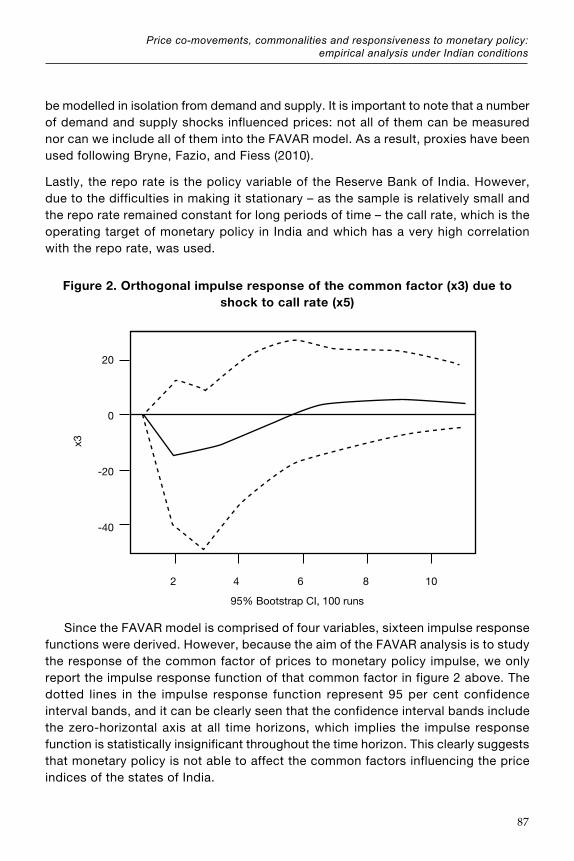
Price co-movements, commonalities and responsiveness to monetary policy: empirical analysis under Indian conditions
87
be modelled in isolation from demand and supply. It is important to note that a number of demand and supply shocks influenced prices: not all of them can be measured nor can we include all of them into the FAVAR model. As a result, proxies have been used following Bryne, Fazio, and Fiess (2010).
Lastly, the repo rate is the policy variable of the Reserve Bank of India. However, due to the difficulties in making it stationary – as the sample is relatively small and the repo rate remained constant for long periods of time – the call rate, which is the operating target of monetary policy in India and which has a very high correlation with the repo rate, was used.
Figure 2. Orthogonal impulse response of the common factor (x3) due to shock to call rate (x5)
Since the FAVAR model is comprised of four variables, sixteen impulse response functions were derived. However, because the aim of the FAVAR analysis is to study the response of the common factor of prices to monetary policy impulse, we only report the impulse response function of that common factor in figure 2 above. The dotted lines in the impulse response function represent 95 per cent confidence interval bands, and it can be clearly seen that the confidence interval bands include the zero-horizontal axis at all time horizons, which implies the impulse response function is statistically insignificant throughout the time horizon. This clearly suggests that monetary policy is not able to affect the common factors influencing the price indices of the states of India.
95% Bootstrap CI, 100 runs
20
0
-20
-40
x3
2 4 6 8 10

Asia-Pacific Sustainable Development Journal Vol. 25, No. 2
88
VI. DISCUSSION OF EMPIRICAL RESULTS AND CONCLUSION
The stationarity test clearly reveals that the food price index and the non-food price index for states under consideration is non-stationary in level, and becomes stationary on first differencing, which implies that these price indices are not mean. Since the non-stationary series with the same order of integration can be cointegrated, the food price and non-food price indices of Indian states were tested for Pedroni’s (1999) panel cointegration. Significant cointegrating relations between food and non-food price indices were observed at all levels (rural, urban and combined). This result authenticates the viewpoint of West and Wong (2014), that co-movements are a central feature of commodity prices, and therefore Central Banks should not decouple price movements into volatile and core components. This part of the empirical result reaffirms the fact that prices follow a form of herd behaviour, and that food price inflation is not temporary, as it breeds into the prices of non-food commodities and vice versa. As a result, every movement in the price index, which is used to estimate the official measure of inflation, warrants policy response.
Second, the Bai and Ng (2004) panel analysis of idiosyncratic and common component analysis further demonstrates that non-stationarity among price indices is due to the common factors influencing them. From this it can be inferred that common factors influencing prices, (which may be demand or supply shocks) might not be of a temporary nature and would thus require structural changes at the micro level.
Third, the impulse response functions derived from the factor augmented vector autoregression analysis throws light on some important aspects of monetary policy and its effectiveness. The insignificant impulse response function, showing the impact of shocks to policy rate among common factors in Indian states, clearly highlight the fact that monetary policy in India is unable to address those factors responsible for fluctuations of prices across the country. This is perhaps one of the reasons behind the differential rates of inflation existing across India.
It can thus be concluded that co-movements among prices of unrelated goods do exist in India. These co-movements are mainly due to the common factors such as political, economic, international or social factors, affecting prices. As a result of these co-movements among unrelated prices, no movement in any price should be ignored by policymakers. Since these common factors among Indian states do not respond to policy, the Reserve Bank of India should seek to identify the sources of fluctuations within states, so that the flexible inflation targeting of India becomes successful in the long run.

Price co-movements, commonalities and responsiveness to monetary policy: empirical analysis under Indian conditions
89
REFERENCES
Alquist, R., and O. Coibion (2013). The comovement in commodity prices: sources and implications. IMF Working Paper, No.13/140. Washington, D.C.: International Monetary Fund. Available from www.imf.org/en/Publications/WP/Issues/2016/12/31/The-Comovement-in-Commodity-Prices-Sources-and-Implications-40633.
Bai J., and S. Ng (2004). A PANIC attack on unit roots and cointegration. Econometrica, vol. 72, No. 4, pp. 1127-1177.
Baffes, J. (2007). Oil spills on other commodities. Resource Policy, vol. 32, No. 3, pp. 126-134.
Baumeister, C., and P. Geert (2011). The role of time-varying price elasticities in accounting for volatility changes in the crude oil market. Journal of Applied Econometrics, vol. 28, No. 7, pp. 1087-1109.
Baumeister, C., and L. Kilian (2012). Real-time forecasts of the real price of oil. Journal of Business and Economic Statistics, vol. 30, No. 2, pp. 326-336.
Bhattacharya, Rudrani, Narhari Rao, and Abhijit Sen Gupta (2014). Understanding food inflation in India. ADB South Asia Working Paper, No. 26. Asian Development Bank. Available from https://www.adb.org/publications/understanding-food-inflation-india.
Bernanke, B.S., J. Boivin, and P. Eliasz (2005). Measuring the effects of monetary policy: a factor-augmented vector autoregressive (FAVAR) approach. Quarterly Journal of Economics, vol. 120, No. 1, pp. 387-422.
Blanchard, O. J., and N. Kiyotaki. (1987). Monopolistic competition and the effects of aggregate demand. American Economic Review, vol. 77, No. 4, pp. 647-666.
Blinder, A. S. (1982). Review of core inflation by Otto Eckstein. Journal of Political Economy, vol. 90, pp. 1306-1309.
Breusch, T. S., and A. R. Pagan (1980). The Lagrange multiplier test and its application to model specifications in econometrics. Review of Economic Studies, vol. 47, No. 1, pp. 239-253.
Bryne, J.P., G. Fazio, and N. Fiess (2010). Primary commodity prices: co-movements, common factors and fundamentals. Journal of Development Economics, vol. 101, pp 16-26.
Calvo, G. A. (1983). Staggered prices in a utility-maximizing framework. Journal of Monetary Economics, vol. 12, No. 3, pp. 383-398.
Chamberlin, E. (1933). The Theory of Monopolistic Competition. Cambridge: Harvard University Press.
Chow, G. C., S. Huang, and L. Niu (2013). Econometric analysis of stock price co-movement in the economic integration of East Asia. Working Papers, Wang Yanan Institute for Studies in Economics (WISE), Xiamen University. Available from www.princeton.edu/~gchow/Econometric%20Analysis%20of%20Stock%20Price%2020111004.pdf.
Cecchetti, S.G., C. M. Nelson, and R. Sonora (2002). Price index convergence among United States cities. International Economic Review, vol. 43, No. 4, pp. 1081-1099.
Deaton, A. (1999). Commodity prices and growth in Africa. Journal of Economic Perspectives, vol. 13, No. 3, pp. 23-40.
Dixit, A., and J. Stiglitz (1977). Monopolistic competition and optimum product diversity. The American Economic Review, vol, 67, No. 3, pp. 297-308.

Asia-Pacific Sustainable Development Journal Vol. 25, No. 2
90
Eckstein, Otto (1981). Core Inflation. Englewood Cliffs: Prentice-Hall.
Hadri, K. (2000). Testing for stationarity in heterogeneous panel data. Econometrics Journal, vol. 3, No. 2, pp. 148-161.
Hall, R. L., and C. J. Hitch (1939). Price theory and business behaviour. Oxford Economic Papers, vol. 2, No. 1, pp. 12-45.
Im, K. S., M. H. Pesaran, and Y. Shin (1997). Testing for unit roots in heterogeneous panels. Mimeo.
Im, K. S., M. H. Pesaran, and Y. Shin (2003). Testing for unit roots in heterogeneous panels. Journal of Econometrics, Vol. 115, pp. 53-74.
India, Ministry of Statistics and Programme Implementation (MOSPI) (2019). Consumer Price Index (CPI) Database. Available from www.mospi.gov.in. Accessed 23 April 2019.
Keynes, J. M. (1936). The General Theory of Employment, Interest and Money. London: Macmillan.
Lucas Robert Jr. (1972). Expectations and the neutrality of money. Journal of Economic Theory, vol. 4, No. 2, pp. 103-124.
Levin, A., C. F. Lin, and C. S. J. Chu (2002). Unit root tests in panel data: asymptotic and finite-sample properties. Journal of Econometrics, vol. 108, No. 1, pp. 1-24.
Manes. E., F. Schneider, and A. Tchetchik (2016). On the boundaries of shadow economy: an empirical investigation. IZA Discussion Paper No. 10067. Bonn: IZA Institute of Labor Economics. Available from www.iza.org/publications/dp/10067/on-the-boundaries-of-the-shadow-economy-an-empirical-investigation.
Moon, H. R., and B. Perron (2004). Testing for a unit root in panels with dynamic factors. Journal of Econometrics, vol. 122, No. 1, pp. 81-126.
Patnaik, A. (2016). Inflation differential and inflation targeting in India. Prajnan, vol. 45, No. 1, pp. 9-24.
Pedroni, P. (1999). Critical values for cointegration tests in heterogenous panels with multiple regressors. Oxford Bulletin of Economics and Statistics, Special Issue, 0305-9049, pp. 653-670. Oxford, United Kingdom: Blackwell. Available from https://pdfs.semanticscholar.org/305e/3d41bb89d64cad1662532952f980a169f3f5.pdf.
Pesaran, M. H. (2007). A simple panel unit root test in the presence of cross section dependence. Journal of Applied Econometrics - Special Issue, vol. 22, No. 2, pp. 265-312.
Pindyck, R. S., and J. J. Rotemberg (1990). The excess co-movement of commodity prices. The Economic Journal, vol. 100, No. 403, pp. 1173-1187.
Pradhananga, M. (2016). Financialization and the rise in co-movement of commodity prices. International Review of Applied Economics, vol. 30, No. 5, pp. 547-566.
Prebisch, R. (1950). The Economic Development of Latin America and its Principal Problems. New York: United Nations. Available from https://repositorio.cepal.org/bitstream/handle/11362/30088/S4900192_en.pdf?sequence=1&isAllowed=y.
Reserve Bank of India (2017). Handbook of Statistics on the Indian Economy. Mumbai. Available from https://rbidocs.rbi.org.in/rdocs/Publications/PDFs/0HANDBOOK2017C9CF31D4B78241C9843272E441CD7010.PDF.
Rich, R., and C. Steindel (2005). A review of core inflation and an evaluation of its measures. Staff Report No. 236. Federal Reserve Bank of New York. Available from www.newyorkfed.org/medialibrary/media/research/staff_reports/sr236.pdf.

Price co-movements, commonalities and responsiveness to monetary policy: empirical analysis under Indian conditions
91
Rotemberg, J. J. (1982). Monopolistic price adjustment and aggregate output. Review of Economic Studies, vol. 49, No. 4, pp. 517-531.
Robinson, J. (1969). The theory of value reconsidered. Australian Economic Papers, vol. 8, No. 12, pp. 13-19.
Said, S.E. and D.A Dickey (1984). Testing for unit roots in autoregressive-moving average models of unknown order. Biometrika, vol. 71, No. 3, pp. 599-607.
Sprinkel, B. W. (1975). 1975: A year of recession, recovery and decelerating inflation. Journal of Business, vol. 48, No. 1, pp. 1-4.
Sraffa, P. (1926). The laws of returns under competitive conditions. The Economic Journal, vol. 36, No. 144, pp. 535-551.
Taylor J. B. (1980). Aggregate dynamics and staggered contracts. Journal of Political Economy, vol. 88 , No. 1, pp. 1-23.
Tobin, J. (1981). The monetarist counter-revolution today - an appraisal. Economic Journal, vol. 91, No. 361, pp. 29-42.
West, K. D., and K. Wong (2014). A factor model for co-movements of commodity prices. Journal of International Money and Finance, vol. 42, pp. 289-309.

Asia-Pacific Sustainable Development Journal Vol. 25, No. 2
92
APPENDIX
Table A.1. Panel cointegration results for the 25 states under consideration
Pedroni residual cointegration test CPI (food) and CPI (non-food) Rural
Within dimensions Statistic Between dimensions Statistic
Panel v-statistic 2.8593
Panel rho-statistic -62.034 Group rho-statistic -70.3814
Panel PP-statistic -16.390 Group PP-statistic -16.1742
Panel ADF-statistic -227.390 Group ADF-statistic -15.9607
Pedroni residual cointegration test CPI (food) and CPI (non-food) Urban
Within dimensions Statistic Between dimensions Statistic
Panel v-statistic 65.24134
Panel rho-statistic -57.4018 Group rho-statistic -53.1677
Panel PP-statistic -12.8914 Group PP-statistic -11.8808
Panel ADF-statistic -14.4973 Group ADF-statistic -11.6376
Pedroni residual cointegration test CPI (food) and CPI (non-food) Combined
Within dimensions Statistic Between dimensions Statistic
Panel v-statistic 13.39335
Panel rho-statistic -107.342 Group rho-statistic -108.045
Panel PP-statistic -27.7450 Group PP-statistic -23.92913
Panel ADF-statistic -107.086 Group ADF-statistic -23.5788
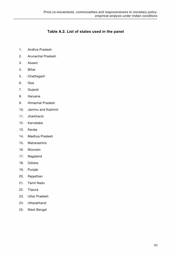
Price co-movements, commonalities and responsiveness to monetary policy: empirical analysis under Indian conditions
93
Table A.2. List of states used in the panel
1. Andhra Pradesh
2. Arunachal Pradesh
3. Assam
4. Bihar
5. Chattisgarh
6. Goa
7. Gujarat
8. Haryana
9. Himachal Pradesh
10. Jammu and Kashmir
11. Jharkhand
12. Karnataka
13. Kerala
14. Madhya Pradesh
15. Maharashtra
16. Mizoram
17. Nagaland
18. Odisha
19. Punjab
20. Rajasthan
21. Tamil Nadu
22. Tripura
23. Uttar Pradesh
24. Uttarakhand
25. West Bengal

Asia-Pacific Sustainable Development Journal Vol. 25, No. 2
94
Methodology
Coss-sectionally augmented Im, Pesaran and Shin test (2007)
Since, a panel of the price indices of the states of India have been used, cross sectional dependence is natural (which was also found using the Pesaran (2004) test and the Breusch and Pagan (1980) test) and so Pesaran’s (2007), cross sectional augmented Im, Pesaran and Shin (CIPS) panel unit root test has been used to test for presence of non-stationarity in the price indices. Unlike the first generation panel unit root tests which were the extensions of Augmented Dickey Fuller Test (ADF) test for cross-sectionally independent panels, Pesaran’s test is a single factor panel unit root test for cross-sectionally dependent panels. For a panel of N cross sections and T time periods the following cross sectional ADF model given in equation (5) below was used by Pesaran (2007).
∆Yit = αi + biYit-1 + ciýt-1 + di∆ýt + εit (2)
Where ý = n-1 ∑ni=1Yit , ∆ý = n-1 ∑n
i=1 ∆Yit (3)
and εit is the regression error.
With the null hypothesis of a unit root, Pesaran (2007) proposed a test based on the t-ratio of the ordinary least squares (OLS) estimate of the estimated bi. The cross sectional averages given in equation (3) are used as proxy for the unobserved common factor. In line with the Im, Pesaran and Shin (IPS) (2003) test, Pesaran proposed the cross sectional augmented version of IPS test.
CIPS = 1/N ∑ni=1 CADFi (4)
Using equation (3) the individual CADF statistics (bi) are estimated and using equation (4), the CIPS statistic is obtained (Patnaik, 2016).
Panel cointegration analysis: Pedroni (1999)
The present study uses the panel cointegration test proposed by Pedroni (1999). In this test, Pedroni (1999) has proposed a residual based test for the null of no cointegration for both homogenous and heterogeneous panels. In particular it covers both between dimension and within dimension residual based test statistic. He derived

Price co-movements, commonalities and responsiveness to monetary policy: empirical analysis under Indian conditions
95
seven panel cointegration test statistics, of which four are based on within dimension and three are based on between dimension. For the within dimension statistic the null hypothesis of no cointegration test is H0: γi = 1 for all i
H0: γi =γ <1 for all i
For between dimension statistic the null hypothesis of no cointegration for the panel is
H0: γi = 1 for all i
H0: γi <1 for all i
The residuals of the hypothesized cointegrating relations, which may be of the form given in the equation (4) are derived first.
Yit = αi +βxit +eit (5)
t i =1....T (is the number of observations in the panel) , and i=1....N (is the number of cross section units used in the panel) The seven test statistics of Pedroni (1999) are :-
The within dimension tests (also called panel cointegration statistics)
(1) Panel υ-statistic (a non-parametric variance ratio test)
(2) Panel ρ-statistic ( a non-parametric statistic similar to Phillips and Perron rho-statistic)
(3) Panel t-statistic ( a non-parametric statistic similar to Phillips and Perron t-statistic)
(4) Panel t-statistic (parametric statistic similar to ADF t-statistic)
Between dimension tests (also called group mean panel cointegration statistic)
(5) Group ρ-statistic (a non-parametric statistic similar to Phillips and Perron t-statistic)
Asia-Pacific Sustainable Development Journal Vol. 25, No. 2
96
(6) Group t-statistic (a non-parametric statistic similar to Phillips and Perron t-statistic)
(7) Group t-statistic (parametric statistic similar to ADF t-statistic) Pedroni (1999)
The panel variance ratio test, under the alternative hypothesis diverges to positive infinity. Since the right tail of normal is used to reject the null hypothesis, large positive values imply that the null is rejected. The other entire statistic diverges to negative infinity under the alternative hypothesis. Since the left tail of normal distribution is used to reject the null hypothesis, large negative values imply that the null of cointegration is rejected.
Panel analysis of idiosyncratic and common components (PANIC): Bai and Ng (2004)
Empirical testing of co-movements in prices requires them to be cointegrated, and cointegration requires the price indices to be non-stationary and integrated of the same order. In recent years, a number of investigators have developed panel based unit root testing (Im, Pesaran and Shin, 1997; Hadri, 2000; Levin, Lin, and Chu, 2002; etc). Most of these tests are based on the assumption of cross sectional independence of panels. Also, most of the panel unit root tests filter out the common factors before testing for unit roots in the data (Pesaran, 2007; Moon and Perron, 2004). However, these common factors may be responsible for the non-stationarity in the panels. Bai and Ng’s (2004) PANIC analysis decomposes the panel data into common and idiosyncratic components and allows the common component to be non-stationary, i.e. it allows for cross-unit cointegration. The Bai and Ng’s (2004), can be explained as follows:-
Let the factor analytic model for the price indices Pi,t be
Pi,t = αit +λi 'Ft+eit i= 1,……..N; and t =1,………T (6)
Where, αit is a polynomial trend function, Ft is an r x1 vector of common factors, and λi is an r x 1 vector of factor loadings. The term λi’ Ft is the common component, while eit are the idiosyncratic components, (the factors are extracted using the principal component method). While all price indices share the same r common factors, λi the factor loadings may differ across indices. The Pi,t series is the sum of deterministic component αit, a common component λi’Ft and an error eit. A factor model with N variables has N idiosyncratic components but a small number of common factors. It will be stationary only if both, the common factor(s) and idiosyncratic factors are

Price co-movements, commonalities and responsiveness to monetary policy: empirical analysis under Indian conditions
97
+ vt
ƒt-i
rt-i
ƒt
rt= Φ (L)
stationary and the common factors can be consistently estimated only if the errors of equation 6 are stationary. For inference, depending on the number of factors PANIC will determine the number of stochastic trends in the common factors. This will be different from the tests on the idiosyncratic errors. The two univariate test are based on the t-test of Said and Dickey (1984), on an augmented regression with suitable lags.
The factor augmented vector autoregression
The FAVAR proposed by Bernanke, Boivin, and Eliasz (2005) modifies the vector autoregression equation involving the observed variables like the repo rate/ call rate with the addition of the set of latent dynamic (common) factors (extracted from the price indices of the states using the method of principal components). The FAVAR model so derived can be shown with the help of the equation (7) given below:-
(7)
Where rt is an m x 1 vector of observed variables including the monetary policy instrument variables the demand and supply shocks and ƒt represents the k x 1 vector of common factors comprising of additional information not contained in rt and derived from the price indices data of the states.


99
MEASURING CREATIVE ECONOMY IN INDONESIA: ISSUES AND CHALLENGES IN DATA COLLECTION
Eni Lestariningsih, Karmila Maharani and Titi Kanti Lestari*
Although creative economy is emerging as an area to be evaluated, establishing a benchmark against which it can be measured is still problematic due to a range of definitional problems, both conceptual and practical. In recent years, many agencies and governments have invested significant effort into collecting data on creative economy, but in many countries, including Indonesia, measuring creative economy remains a challenge. Data collection on creative economy has been conducted twice in Indonesia, initially through surveys undertaken in 2016 and then in a compilation of the 2016 Economic Census. The data collection used a common classification system to identify the five-digit Indonesia Standard Industrial Classification (KBLI) regarded as creative economy. Out of a total of 1,573 five-digit KBLI codes, there are 223 which are identified as creative economy activities. However, this approach remains unstandardized in terms of concept definitions, data collection procedures, methods of analysis and common classification systems. This paper highlights the numerous limitations in current creative economy measurement in Indonesia, identifying issues and challenges in data collection and creative economy measurement processes that are needed to support the Sustainable Development Goals.
JEL classification: O10
Keywords: creative economy, Sustainable Development Goals
* Eni Lestariningsih, Statistics Indonesia, Badan Pusat Statistik, Jakarta, Indonesia (email:[email protected]). Karmila Maharani (email:[email protected]); Titi Kanti Lestari (email:[email protected]).

Asia-Pacific Sustainable Development Journal Vol. 25, No. 2
100
I. INTRODUCTION
Culture, innovation and creativity are now acknowledged as driving forces of the new economy. Organizations and even economic regions that embrace creativity generate significantly higher revenue and provide greater stability for the future. According to UNESCO, creative economy is “one of the most rapidly growing sectors of the world economy and a highly transformative one in terms of income generation, job creation and export earnings” (UNDP and UNESCO, 2013, p. 10). Creative economy sectors can contribute considerably to growth and prosperity, especially for developing countries seeking to diversify their economies and build resilience.
It is therefore essential to measure creative economy and its impact on the overall economic system, and the collection of quality statistics is critical to achieving the associated targets of the Sustainable Development Goals (SDGs). The central aim of the SDGs is to leave no one behind. They encompass the interlinkages among the three dimensions of economic growth, social development and environmental sustainability (Lestariningsih, Gusnisa and Maharani, 2017). The measurement of creative economy will thus enable evidence-based policymaking to support the SDGs.
Providing creative economy statistics undoubtedly requires extended processes and standardized procedures. As the importance of creative economy is increasingly appreciated, the necessity for quantifying its value and comparability is also growing. As stated by the World Economic Forum “the economic significance of the creative economy is indisputable; however, its impact is broader than can be measured simply by economic output” (World Economic Forum, 2016, p. 10).
The complexity of establishing criteria to measure creative economy is due to a range of conceptual and practical codification issues. Lack of standardization regarding definitions, data collection procedures, analysis and dissemination of data, and common classification systems all make regional comparison problematic.
Creative economy has become the new source of economic growth in Indonesia, but it requires unambiguous methods of evaluation in order to provide good quality data. It is anticipated that measurement of creative economy by survey will become more systematic and more accurate, following the life cycle survey, consisting of client liaison, planning, survey development, sample design, data processing, estimation, analysis, dissemination and evaluation. There are, however, still many hurdles to overcome in measuring the creative economy in Indonesia, and initially there is need for a framework, with standardization of concept and methodology in order to explore current insights for evidence of contribution towards sustainable development.

Measuring creative economy in Indonesia: issues and challenges in data collection
101
This study highlights numerous limitations in current creative economy measurement practices in Indonesia, as well as the issues and challenges arising out of the collection of data and the development of a creative economy contribution model as an evidence base to support the Sustainable Development Goals.
II. CREATIVE ECONOMY: CONCEPTS AND IMPORTANCE TO DEVELOPMENT
Creative economy has become an economic growth booster in many countries, and is unique in that it is created from an unlimited resource – ideas. Not only is the resource unlimited, it also contributes high added value to goods and services. The United Kingdom Department for Digital, Culture, Media and Sport defined creative economy as “those industries which have their origin in individual creativity, skill and talent, and which have a potential for wealth and job creation through the generation and exploitation of intellectual property” (United Kingdom, Department for Digital, Culture, Media and Sport, 2001, p. 4).
Another definition of creative economy is provided by UNCTAD: “creative economy is an emerging concept dealing with the interface between creativity, heritage, economics and technology in a contemporary world dominated by images, sounds, texts and symbols” (UNCTAD, 2018). This definition emphasizes four determinants of creative economy: creativity, heritage, economics and technology.
In addition to boosting growth, creative economy contributes to sustainable development. It is becoming increasingly accepted that “sustainability” has a broader scope beyond its application to the environment. It is related to both tangible and intangible cultural capital, as part of creative economy, which is related to sustainable development (UNCTAD, 2010). Cultural sustainability implies a development process that maintains all types of cultural assets, from minority languages and traditional rituals to artworks, artefacts and heritage buildings and sites. It is creative industries that provide the services and investments necessary for culturally sustainable development paths to be followed. It includes industries related to creativity, art and culture, whose contribution can be characterized based on creative economy macroeconomic indicators, social culture development and environmental sustainability.
The development of creative economy has contributed to the United Nations Sustainable Development Goals, in particular: Goal 1 – “Eradicate extreme poverty for all people everywhere”; Goal 8 – “Promote sustained, inclusive and sustainable economic growth, full and productive employment and decent work for all”; and Goal 9 – “Build resilient infrastructure, promote inclusive and sustainable industrialization and foster innovation” (UNDP, 2015, pp. 10, 12).

Asia-Pacific Sustainable Development Journal Vol. 25, No. 2
102
In this case, the essence of Goal 1 can be achieved through social and cultural elements, such as education, health and gender empowerment activities, which are closely related to poverty eradication. For example, an improvement in creative economy could enable an increase in living standards, translating into a higher proportion of the population living above the poverty line, as reflected in indicator 1.2.1 (proportion of population living below the national poverty line, by sex and age). Many creative economy activities emerge from young people, and observations have shown that many entrepreneurs are women.
For Goal 8 (sustainable economic growth), there are three indicators related to the development of creative economy, they are: 8.1.1 (annual growth rate of real gross domestic product per capita); 8.3.1 (proportion of informal employment in non-agricultural occupations, by gender); and 8.9.2 (number of jobs in tourism industries as a proportion of total jobs and growth rate of jobs, by gender). These three indicators show that a developing creative economy will raise gross domestic product (GDP) per capita, absorb a greater number of informal1 employees and generate more jobs in creative fields related to tourism.
The measurement of innovation indicators can also be linked to Goal 9 (build resilient infrastructure, promote inclusive and sustainable industrialization and foster innovation). Creativity is one of the main criteria in research and development, especially in Target 9.5: enhance scientific research, upgrade the technological capabilities of industrial sectors in all countries, particularly developing countries including, by 2030, encouraging innovation and substantially increasing the number of workers and spending on both public and private research and development. Here, there are two relevant indicators: Indicator 9.5.1 – “Research and development expenditure as a proportion of GDP”; Indicator 9.5.2 – “Researchers (in full-time equivalent) per million inhabitants”. More expenditure and researchers will thus result in more innovative products, goods and services.
III. MEASURING THE CREATIVE ECONOMY IN INDONESIA: METHODOLOGY, RESULTS, AND SYNTHESIS
Many countries have collected data on creative economy, particularly: Australia (surveys of industries); Canada (Culture labour-force survey, Statistics Canada); Finland, France and Italy (creative sector statistics collected, national statistical agencies); the Philippines (extracts from national statistical agency); and the United Kingdom and Singapore (extracts of information from data collected by businesses at 4-5 digit
1 Informal employees include: (1) self-employment, (2) temporary workers / unpaid labourers, (3) free workers in agriculture, (4) free workers in non-agriculture, and (5) family / unpaid workers.

Measuring creative economy in Indonesia: issues and challenges in data collection
103
International Standard Industrial Classification (ISIC) level. Some relevant statistics related to specific indicators of the creative economy could also be collected from gross value added, number of businesses, total employment and exports of creative economy. However, there is still little agreement on a methodology for measuring creative industries (UNCTAD, 2015; Joffe, 2012).
In the case of Indonesia, creative economy is officially measured by Badan Pusat Statistik (BPS), the national statistics agency of the Indonesian government. Measurements have been conducted twice, in 2016 and 2017. In 2016, a purposive survey was conducted with regard to creative economy, entitled Special Survey of Creative Economy (Survei Khusus Ekonomi Kreatif 2016) (BPS, 2017d), while in 2017 the creative economy was measured through the Economic Census (BPS, 2017a). The creative economy statistics resulting from Survei Khusus Ekonomi Kreatif 2016 and the Economic Census are publicly available on the website of Indonesia Creative Economy Board.2 They are also available as a printed version in BPS-Statistics Indonesia.
In Indonesia, as in the United Kingdom and Singapore, the five-digit International Standard Industrial Classification (ISIC) code is used for identifying creative economy activities. Indonesia has established its own creative economy ISIC codes, called Klasifikasi Baku Lapangan Usaha Indonesia (KBLI), Indonesia Standard Industrial Classification (ISIC) or KBLI-ISIC . As a definition of creative economy, Badan Pusat Statistik (BPS) – Statistics Indonesia, use the creative economy concept from UNCTAD (2015), which emphasizes four determinants of creative economy: creativity, heritage, economics and technology. Using these four determinants, BPS engaged with people in creative businesses in order to refine its information and understanding about creative economy activities, after which creative economy codes were extracted from the KBLI-ISIC, resulting in 223 creative economy codes out of the 1,573 five-digit Indonesia Standard Industrial Classification.
Creative economy in Indonesia is also measured and defined by 16 creative industries. Based on Presidential Decree Number 72, 2015 (Indonesia, 2015), creative economy in Indonesia covers 16 creative industries: (1) Architecture; (2) Interior design; (3) Visual communication design; (4) Product design; (5) Film, animation and video; (6) Photography; (7) Craft; (8) Culinary arts; (9) Music; (10) Fashion; (11) Application and game development; (12) Publishing; (13) Advertising; (14) Television and radio; (15) Performing arts; and (16) Fine arts. These 223 five-digit KBLI-ISIC are spread over the 16 creative industries and categories of International Standard Industrial Classification Revision 4 (DESA, 2008) which are presented in table 1:
2 Badan Ekonomi Kreatif Indonesia website is available from www.bekraf.go.id.

Asia-Pacific Sustainable Development Journal Vol. 25, No. 2
104
Table 1. Number of five-digit creative economy KBLI for each creative industry
No. Creative industriesISIC Revision 4
category/sectionKBLI-ISIC
number
1 Architecture M 2
2 Interior design M, P 2
3 Visual communication design M, P 2
4 Product design M, N, P 3
5 Film, animation and video C, J, P 9
6 Photography M, P, R 7
7 Craft C, G 72
8 Culinary arts C, G, I 32
9 Music C, G, J, N, P, R 9
10 Fashion C, G, P 19
11 Application and game developer J, M, R 13
12 Publishing C, G, J, M, R 17
13 Advertising M 5
14 Television and radio J 5
15 Performing arts N,P,R 10
16 Fine arts G, M, P, R 16
Total 223
Source: DESA (2008) and BPS (2016f).
Note: Category/section in ISIC Revision 4 for Creative Economy
C. Manufacturing
G. Wholesale and retail trade; repair of motor vehicles and motorcycles
I. Accommodation and food service activities
J. Information and communication
M. Professional, scientific and technical activities
N. Administrative and support service activities
P. Education
R. Arts, entertainment and recreation
Based on the creative economy KBLI-ISIC codes, the measurement of creative economy in Indonesia has been implemented through the Special Survey of Creative Economy (Survei Khusus Ekonomi Kreatif) (BPS, 2016e) by applying the non-probability sampling method – purposive sampling – due to the unavailability of an existing sampling frame on creative economy. Purposive sampling was applied by choosing, as the unit sample, businesses which fulfill the following criteria: (i) The businesses are matched with one or more of the 223 creative economy KBLI-ISIC;

Measuring creative economy in Indonesia: issues and challenges in data collection
105
and (ii) the nature of the businesses’ activities are indicative of creative concept, such as creativity, heritage, economics and technology. The number of samples in the Survey was selected based on these two criteria, and therefore businesses outside the two criteria will be excluded.
As non-probability sampling was used in the Survey, the results were not estimated for the overall population, but became the profile of creative businesses. Some information was collected through the Survey, such as the number of businesses engaging in the creative economy sector, gross revenue in creative economy businesses and total employment in creative economy businesses.
The other macroeconomic indicators in creative economy were also presented in 2016, namely export of creative products (BPS, 2016b), creative workers (BPS, 2016d) and gross domestic product of the creative economy (BPS, 2016c). Each indicator has its own methodology in which to arrive at an estimated value.
Furthermore, current measurement of the Indonesian creative economy in 2017 utilized results from the Economic Census, and the methodology was improved by basing the sampling frame on it. The frame was developed by matching the creative economy KBLI-ISIC codes with businesses in the economic census frame. In this case, it was found that the total number of creative economy businesses in Indonesia was about 8.2 million, and this became the framework for creative economy measurement. Based on this framework, a study was conducted to identify some characteristics of a creative economy business profile, such as: (1) gender of employer; (2) start-up businesses; (3) entity (legal) status; (4) preparation of financial reports; (5) business’s network; (6) employment; (7) internet presence; (8) engagement in e-commerce; (9) franchise status; and (10) gross revenue.
Based on Indonesian experience, it is important to formulate the process by which to standardize measurement of the creative economy. In this paper, we make some effort to document the processes for measuring creative economy in Indonesia as shown in figure 1.

Asia-Pacific Sustainable Development Journal Vol. 25, No. 2
106
Figure 1. Process for measuring creative economy in Indonesia
Goal 1 Eradicate extreme poverty for all people everywhere
Indicator 1.2.1 Proportion of population living below the national poverty line, by sex and age
Goal 8 Promote sustained, inclusive and sustainable economic growth, full and productive employment and decent work for all
CREATIVEECONOMY
START
SDGs
Fine arts
Sampledesign
GDP
Employment
Export
Survey
development
Plan
ning
Clie
nt li
aiso
n
Datacollection
Processing
Estimation
Analysis
16
Interiordesign
2
Productdesign
3
Photography
6
Craft
7
Culinary arts
8
Music
9
Fashion
10
Advertising
12Publishing
13
TV & radio
14
Performingarts
15
Application &game
developer
11
Visualcommunication
design
4
Film, animation,and video
5
Architecture
1
Number of creativebusiness
Dissem
inat
ion
Evaluation

Measuring creative economy in Indonesia: issues and challenges in data collection
107
CREATIVEECONOMY
START
SDGs
Fine arts
Sampledesign
GDP
Employment
Export
Survey
development
Plan
ning
Clie
nt li
aiso
n
Datacollection
Processing
Estimation
Analysis
16
Interiordesign
2
Productdesign
3
Photography
6
Craft
7
Culinary arts
8
Music
9
Fashion
10
Advertising
12Publishing
13
TV & radio
14
Performingarts
15
Application &game
developer
11
Visualcommunication
design
4
Film, animation,and video
5
Architecture
1
Number of creativebusiness
Dissem
inat
ion
Evaluation
1) Indicator 8.1.1 Annual growth rate of real GDP per capita
2) Indicator 8.3.1 Proportion of informal employment in non-agriculture employment, by sex
3) Indicator 8.9.2 Number of jobs in tourism industries as a proportion of total jobs and growth rate of jobs, by sex.
Goal 9 Build resilient infrastructure, promote inclusive and sustainable industrialization and foster innovation
1) Indicator 9.5.1 Research and development expenditure as a proportion of GDP
2) Indicator 9.5.2 Researchers (in full-time equivalent) per million inhabitants
Figure 1 describes creative economy coverage and the phase of data collection for measuring creative economy in Indonesia. The 16 Indonesian creative economy industries are measured using a standard survey life cycle, which starts from client liaison, planning, survey development, sample design, data collection, processing, estimation, analysis, dissemination and evaluation. The resulting data collection is beneficial for describing the creative economy’s contribution to sustainable development, particularly in supporting Sustainable Development Goals 1, 8 and 9. However, this approach is still not standardized, particularly regarding the determination of concept definitions for the 16 Indonesian creative economy activities.
Some of the creative economy insights emerging from the Special Survey of Creative Economy (Survei Khusus Ekonomi Kreatif) (BPS, 2016f) could support the improvement of SDGs indicator 1.2.1 “proportion of population living below the national poverty line, by sex and age”, specifically:
a) The number of creative economy businesses in Indonesia in 2016 is 8.2 million.
b) The majority of creative economy entrepreneurs are women (55 per cent).
c) Small and microbusinesses are an important part of the creative economy in Indonesia. Almost 92 per cent of creative industries in Indonesia are from small or microestablishments – Usaha Mikro Kecil.
d) The average educational attainment of creative economy entrepreneurs is post-secondary education.

Asia-Pacific Sustainable Development Journal Vol. 25, No. 2
108
This data can be related to SDG indicators to show how improvement in the creative economy can raise the standard of living in the general population.
Other creative economy data arising from the Indonesia Economic Census 2016 (BPS, 2017a) may be connected to three SDG indicators: Indicator 8.1.1 (Annual growth rate of real GDP per capita); Indicator 8.3.1 (Proportion of informal employment in non-agriculture employment, by sex); and Indicator 8.9.2 (Proportion of jobs in sustainable tourism industries out of total tourism jobs). Some of the data relating to these indicators are as follows:3
a) The proportion of start-up businesses in the creative economy is 19.8 per cent.
b) The number of creative economy businesses in Indonesia in 2016 was 8.2 million.
c) The creative economy of Indonesia is driven by three dominant industries: Culinary arts, fashion, and arts and crafts (Kriya).
d) Most (92.6 per cent) creative economy businesses have revenues under 300 million rupiah per annum ($20,690).
e) The majority of businesses in creative economy tend to be microenterprises, with 1-4 employees (95.6 per cent).
f) The contribution of the creative economy towards national GDP in 2016 was 7.4 per cent (BPS, 2017c).
This data can be related to the three SDG indicators which suggest that development of creative economy will raise the per capita GDP, absorb a greater number of informal employees, and generate more jobs in creative fields.
Other creative economy data which may be connected to SDG Indicator 9.5.1 (research and development expenditure as a proportion of GDP) is as follows:
a) The creative industries conducting research and development are application and game development (51.4 per cent), television and radio (46.2 per cent) and visual communication design (44.9 per cent).
b) The contribution of creative economy to GDP in 2016 was 922.6 trillion rupiah ($63.6 billion) (BPS, 2017c).
c) The influence of the creative economy was felt mainly in the domestic market. Overseas sales accounted for only 8.4 per cent of total output, whereas export of creative economy commodities in 2016 was $20 billion (BPS, 2017b).
3 Exchange rate of 1 United State dollar to 14,500 Indonesian rupiah, as of December 2018.

Measuring creative economy in Indonesia: issues and challenges in data collection
109
This data can be related to SDG indicators to clarify that creativity is a driver of innovation. Improving creativity can thus encourage innovation in general, and specifically research and development.
IV. ISSUES AND CHALLENGES
The measurement of creative economy is generally challenging – not just in Indonesia – and establishing a benchmark to measure creative economy is still problematic due to a range of categorization issues, both conceptual and practical. In recent years, many agencies and governments have put much effort into collecting data on the creative economy (WIPO, 2013). Creative economy data collection has been conducted twice in Indonesia: the Creative Economy Survey in 2016, and from the Economic Census in 2017.
Sample numbers in the 2016 Creative Economy Survey are 6,000 businesses from 16 creative industries in 57 cities and districts in 34 provinces of Indonesia, while in 2017, the compilation of creative economy data utilized 2016 Economic Census data (BPS, 2017a). The 2016 Economic Census covered all businesses in all sectors of the Indonesian economy, except the agricultural sector (KBLI-ISIC category A), government administration sector (KBLI-ISIC category O) and household activities as employer sectors (KBLI-ISIC category T).
The issues and challenges in creative economy data collection in Indonesia can be summarized based on our experience in 2016 and 2017 as presented below:
Lack of standardized definition
Development of the creative economy has been hampered by multiple definitions and the lack of a consistent approach on how to classify creative activity. The first limitation is the definition of creative economy itself. At an early stage of defining creative economy industrial classification codes (KBLI-ISIC), the National Statistics Office of Indonesia discussed with the Creative Economy Agency of Indonesia (Badan Ekonomi Kreatif) and people working in creative businesses how to receive more information and refine the definition of creative economy generally, and also creativity in each sector. The very intangibility of creativity requires the application of strict criteria for measurement. Each business’s criteria of what it means to be creative must be precisely defined in order to delineate which workers and activities can be classified as creative. This process of classification was also evident in the fast-changing communication, cultural and content industries. The fluidity of definitions further complicates understanding and measurement of creative economy. In future, the KBLI could be revised to take account of developments in creative industries, but at present creative economy classification still differs among countries, and international standards and definitions are not yet available.

Asia-Pacific Sustainable Development Journal Vol. 25, No. 2
110
No sampling frame
Generating statistics of creative economy is still new for Indonesia, and the quality of statistics is dependent on the availability of a reliable sampling frame. This issue was addressed in 2016, when Statistics Indonesia conducted a Creative Economy Survey 2016 (BPS, 2016f) in 34 provinces. The sample selection was solely based on non-probability sampling, due to the unavailability of a framework for creative economy businesses in 2016.
In Indonesia, the framework was based on the Economic Census 2016, which identified the businesses matching 223 five-digit classifications in KBLI-ISIC. However, the list of creative economy businesses in the Economic Census frame is quite volatile, due to the lack of standardization of concept and definition in the creative economy KBLI-ISIC codes.
Creative industry classification does not correspond well to the standard creative industries.
With a standard industrial classification approach, one of the issues is that KBLI-ISIC codes can be relevant across many creative industries. Within the 223 five-digit KBLI-ISIC codes, there are 14 codes that belong to more than one creative industry, as shown in table 2.
Indicators of creative economy in Indonesia are based on 16 creative industries, with some limitation of statistics due to lack of standardization in the concept and methodology.
Challenges
All of the creative economy measurements have been based on the industrial classification approach, using the 223 five-digit KBLI-ISIC in creative economy, but despite this, more creative people work outside the creative industries than within them. One of the challenges in measuring creative economy in Indonesia is using a variety of approaches, such as occupation data. The disaggregation of creative economy data is also challenging, as it is necessary to extrapolate statistics based on geographic area, urban-rural classification, the 16 creative industries, gender and other socioeconomic indicators.
These issues and challenges imply that the approach of measuring creative economy needs to be broad, and that data collection must be standardized across all countries, so as to ensure a sustainable database for supporting the SDGs.

Measuring creative economy in Indonesia: issues and challenges in data collection
111
Table 2. Five-digit KBLI-ISIC code crosses with more than one creative industries
No Codes Title Creative industries
1 58200 Publishing software • Application and game developer; • Publishing
2 59202 Music publishing activity and music books
• Music; • Publishing
3 70203 Public relation activity • Advertising; • Fine arts
4 70204 Investment consulting activities and futures trading
• Application and game developer; • Fine arts
5 70209 Consultation activities other management
• Advertising; • Fine arts
6 74100 Special design activities • Interior design; • Communication visual design;• Product design
7 85420 Cultural education • Photography; • Performing arts; • Music; • Fine arts
8 85497 Private technical education • Interior design; • Communication design visual; • Product design
9 85499 Other private education • Movies, animations, and videos; • Fashion; • Performing art; • Fine art
10 90002 Art workers' activities • Photography; • Music; • Application and game developer; • Performing arts; • Fine arts
11 90006 Arts facility operational activities • Photography; • Performing arts
12 90009 Activities entertainment, arts and other creativity
• Photography; • Performing arts
13 91021 Government-managed museum • Photography; • Fine arts
14 91022 Privately-managed museum • Photography; • Fine arts
Source: Indonesia, Badan Pusat Statistik (2016a).

Asia-Pacific Sustainable Development Journal Vol. 25, No. 2
112
V. CONCLUSION
This paper has sought to highlight some of the issues and challenges faced by Indonesia in measuring creative economy, and utilizing that measurement to support SDGs. Based on this goal, it may be concluded that:
(a) Creative economy contributes to sustainable development, which can be seen particularly in the Sustainable Development Goals 1, 8 and 9.
(b) Creative economy in Indonesia is officially measured by National Statistics Office of Indonesia. This measurement has been conducted twice, in 2016 and 2017. Five-digit Indonesia Standard Industrial Classification Codes (KBLI) of creative economy, built by Indonesia, were used as the key for identifying creative businesses. There are 223 five-digit KBLI-ISIC of creative economy in Indonesia.
(c) Establishing a benchmark to measure the creative economy is problematic. Some of the issues are lack of standardized definitions for creative economy, no sampling frame and creative industry classification (KBLI codes) that do not correspond well to standard creative industry criteria.
Other challenges to measuring creative economy in Indonesia are using a different basis, such as occupation, and disaggregation of data based on geographic area, urban-rural, 16 industries of creative economy, gender and other indicators.
Despite many issues and challenges, measuring creative economy remains important to economic development in Indonesia. Indonesia will continuously improve the provision of creative economy data, as a benchmark to support the Sustainable Development Goals.

Measuring creative economy in Indonesia: issues and challenges in data collection
113
REFERENCES
Indonesia (2015). Presidential Decree Number 72. Jakarta.
Indonesia, Statistics Indonesia, Badan Pusat Statistik (BPS) (2016a). Report on Analysis of Classification of Creative Economy Activities in KBLI 2015. Jakarta.
______ (2016b). Report on Analysis of Creative Economy Export in 2010-2015. Jakarta.
______ (2016c). Report on Analysis of Creative Economy GDP in 2010-2015. Jakarta.
______ (2016d). Report on Analysis of Creative Economy Workforce in 2010-2015. Jakarta.
______ (2016e). Report on Analysis of Harmonization of KBLI 2015-HS 2012 for 16 (Sixteen) Industries Creative Economy. Jakarta.
______ (2016f). Report on Creative Economy Business Profile 2016 based on SKEK 2016. Jakarta.
______ (2017a). Report on Creative Economy Business Profile in 16 Creative Economy Industries Based on Economic Census 2016 (SE2016). Jakarta.
______ (2017b). Report on Creative Economy Export in 2010-2016. Jakarta. Available from www.bekraf.go.id/pustaka/page/24-ekspor-ekonomi-kreatif-2010-2016.
______ (2017c). Report on Creative Economy GDP in 2014-2016. Jakarta. Available from www.bekraf.go.id/pustaka/page/67-laporan-penyusunan-pdb-ekraf-5-provinsi-2010-2016-menurut-lapangan-usaha.
______ (2017d). Report on Creative Economy Workforce in 2010-2016. Available from Available from http://www.bekraf.go.id/pustaka/page/55-tenaga-kerja-ekonomi-kreatif-2011-2016.
Joffe, Avril (2012). Policy-making for the creative and cultural industries. Presentation to UNESCO Capacity Building Program – Africa.
Lestariningsih, E., S. Gusnisa, and K. Maharani (2017). Legal setting for the development of interagency sectoral statistics database (ISSD). Paper presented at Asia-Pacific Economics Statistics Week, 22 - 26 May 2017. BPS-Statistics Indonesia. Available from https://drive.google.com/file/d/0ByEfoVVpdu29NE5iS3BpYi1WTTg/view.
United Kingdom, Department for Digital, Culture, Media and Sport (DCMS) (2001). Creative Industries Mapping Documents. United Kingdom: DCMS. Available from https://assets.publishing.service.gov.uk/government/uploads/system/uploads/attachment_data/file/183544/2001part1-foreword2001.pdf.
United Nations, Department of Economic and Social Affairs (DESA) (2008). International Standard Industrial Classification of All Economic Activities Revision 4. New York. Available from https://unstats.un.org/unsd/publication/seriesm/seriesm_4rev4e.pdf.
United Nations Conference on Trade and Development (UNCTAD) (2010). Creative Economy Report 2010: A Feasible Development Option. Geneva. Available from https://unctad.org/en/pages/PublicationArchive.aspx?publicationid=946
______ (2015). Creative Economy Outlook and Country Profiles: Trends in International Trade in Creative Industries. Geneva. Available from https://unctad.org/en/PublicationsLibrary/webditcted2016d5_en.pdf.
______ (2018). UNCTAD’s work on the Creative Economy. Available from https://unctad.org/en/Pages/DITC/CreativeEconomy/Creative-Economy.aspx.

Asia-Pacific Sustainable Development Journal Vol. 25, No. 2
114
United Nations Development Programme (UNDP) (2015). Report on Indicators and Data Mapping to Measure Sustainable Development Goals (SDGs) Targets: Case of Indonesia 2015. Jakarta. Available from www.id.undp.org/content/indonesia/en/home/library/environment_energy/indicators-and-data-mapping-to-measure-sustainable-development-g.html.
United Nations Development Programme (UNDP), and United Nations Educational Scientific and Cultural Organization (UNESCO) (2013). Creative Economy Report 2013 Special Edition: Widening Local Development Pathways. New York: UNDP and UNESCO. Available from www.unesco.org/culture/pdf/creative-economy-report-2013.pdf.
World Economic Forum (2016). White Paper: Factors for Enabling the Creative Economy. Geneva. Available from www3.weforum.org/docs/WEF_2016_WhitePaper_Enabling_the_Creative_Economy.pdf.
World Intellectual Property Organization (WIPO) (2013). Study on the Economic Contributions of Copyright and Related Rights Industries in Indonesia. Geneva. Available from www.wipo.int/export/sites/www/copyright/en/performance/pdf/econ_contribution_cr_id.pdf.

115
ASIA-PACIFIC SUSTAINABLE DEVELOPMENT JOURNAL SUBMISSION GUIDELINES
The Asia-Pacific Sustainable Development Journal (APSDJ) is based on recognition of the interconnected and multidisciplinary nature of sustainable development. Published biannually by the United Nations Economic Commission for Asia and the Pacific, it is intended to stimulate debate and assist in the formulation of evidence-based policymaking in the Asia-Pacific region towards the implementation of the 2030 Agenda for Sustainable Development.
APSDJ welcomes the submission of original contributions on themes and issues related to sustainable development that are policy-oriented and relevant to Asia and the Pacific. The articles should be centred on discussing challenges pertinent to one or more dimensions of sustainable development, policy options and implications and/or policy experiences that may be of benefit to the region.
Authors familiar with the Asia-Pacific region are encouraged to submit their work. All manuscripts will undergo a rigorous double-blind peer-review process.
1. Manuscripts
All materials submitted for the consideration of the Editorial Board should be in English. The manuscripts should be typed, double-spaced, on one side of white A4 paper. They should not exceed 8,000 words, including tables, figures, references and other materials and include a short abstract (200 words) of the issues addressed and the most important policy-related findings.
Manuscripts are accepted on the understanding that they may be edited. Contributors are required to sign a consent form verifying that their articles are original and have not been published in any other publications or refereed journal(s).
All manuscripts will be submitted to double-blind peer review by professionals in the field. The name(s) of the author(s) or other identifying information should, therefore, be placed only on the title page in order to preserve anonymity. The title page should also include such information as institutional affiliation(s), complete mailing address, telephone number and the email of the author(s).
Manuscripts should be sent by email to the chief editors of APSDJ at [email protected].
2. Tables and figures
All tables and figures should be numbered consecutively with Arabic numbers. Each table should be typed double-spaced. Tables and figures should be planned to fit the proportions of the printed page. Full information on the source(s) should appear below the table or figure, followed by notes, if any, in lower-case letters.
Once a manuscript is accepted for publication, the author(s) will be asked to supply figures, tables and charts, preferably in Microsoft Excel or any major spreadsheet program.

Asia-Pacific Sustainable Development Journal Vol. 25, No. 2
116
3. Footnotes and quotations
Footnotes, if any, should be numbered consecutively with superscript Arabic numerals. They should be typed single-spaced and placed at the bottom of each page. They should not be used solely for citing references.
Quotations should be double-spaced. A copy of the page(s) of the original source of the quotation, as well as a copy of the cover page of that source should be provided.
4. References
Authors should ensure that there is a complete reference for every citation in the text. References in the text should follow the author-date format, followed, if necessary, by page numbers, for example, Becker (1964, pp. 13-24). List only references that are cited in the text or footnotes. References, listed alphabetically, should be typed double-spaced on a separate page in the following style:
Sen, Amartya (2009). The Idea of Justice. Cambridge, Mass: Harvard University Press.
Husseini, Rana (2007). Women leaders attempt to bridge East-West cultural divide. Jordan Times, 9 May.
Krueger, Alan B., and Lawrence H. Summers (1987). Reflections on the inter-industry wage structure. In Unemployment and the Structure of Labour Markets, Kevin Lang and Jonathan S. Leonard, eds. London: Basis Blackwell.

United Nations publications may be obtained from bookstores and distributors throughout the world.Please consult your bookstore or write to any of the following:
Customers in: America, Asia and the Pacific
Email: [email protected]: shop.un.orgTel: +17036611571Fax: + 1 703 996 1010
Mail Orders to:United Nations PublicationsPO Box 960Herndon, Virginia 20172United States of America
Customers in: Europe, Africa and the Middle East
United Nations Publicationsc/o Eurospan GroupEmail: [email protected]: un.org/publicationsTel: +44 (0) 1767 604972Fax: +44(0) 1767 601640
Mail orders to:United Nations PublicationsPegasus Drive, Stratton Business ParkBigglewade, Bedfordshire SG 18 8TOUnited Kingdom
For further information on this publication, please address your enquiries to:
Chief EditorsAsia-Pacific Sustainable Development Journal
Social Development Division and Macroeconomic Policy and Financing for Development DivisionUnited Nations Economic and Social Commission for Asia and the Pacific
United Nations Building, Rajadamnern Nok AvenueBangkok 10200, ThailandEmail: [email protected]
For more details, please visit www.unescap.org/apsdj.

ISBN 978-92-1-120789-7
19-0
0370
� e Asia-Paci� c Sustainable Development Journal (APSDJ) is a rebranded publication issued by the Economic and Social Commission for Asia and the Paci� c (ESCAP). It builds on the success of two former ESCAP journals – the Asia-Paci� c Population Journal, launched in 1986, and the Asia-Paci� c Development Journal, launched in 1994.
APSDJ is based on recognition of the interconnected and multidisciplinary nature of sustainable development. Published biannually, it aims to stimulate debate and assist in the formulation of evidence-based policymaking in the Asia-Paci� c region towards the implementation of the 2030 Agenda for Sustainable Development.
Vol. 25, N
o. 2, Decem
ber 2018