Embed Size (px)
Citation preview

Diss. ETH No. 16427
VLSI Circuits for MIMOCommunication Systems
A dissertation submitted to the
SWISS FEDERAL INSTITUTE OF TECHNOLOGYZURICH
for the degree of
Dr. Sc. Techn.
presented by
ANDREAS BURG
Dipl. El. Ing. ETHborn 26. September 1975citizen of Germany
accepted on the recommendation of
Prof. Dr. Wolfgang Fichtner, examinerProf. Dr. Markus Rupp, co-examiner
2006


Acknowledgments
First, I would like to thank my advisor Prof. Dr. Wolfgang Ficht-ner for his encouragement and support, for his faith in my work, andfor providing an excellent research environment. I also gratefully ac-knowledge Prof. Dr. Markus Rupp who was the co-examiner for mythesis. I always highly appreciated his guidance, his continuous sup-port, and the great collaboration we had since I started working oncommunication systems back in the year 2000 at Lucent.A very special thanks goes to Prof. Dr. Helmut Bolcskei from theCommunication Theory Group (CTG) at ETH. The successful, closecollaboration with him and his group is the proof to me that the keyto achieving the highest performing circuits for signal processing liesin understanding both algorithm and VLSI implementation aspectsand in a mutual effort of specialists from both areas. The numerousdiscussions with him and his advice have been an invaluable contri-bution to my effort in further developing my understanding of signalprocessing algorithms and information theory. Also from the CTG, Iwould like to thank my colleague and friend Moritz Borgmann for ournumerous fruitful collaborations and for many invaluable discussions.At the Integrated Systems Laboratory (IIS) I would like to thankDr. Norbert Felber and, from the Microelectronics Design Center,Dr. Hubert Kaeslin for introducing me into the field of digital VLSIdesign and for encouraging me to start my PhD work in this excitingfield. I am also extremely grateful to my colleagues from the MIMOgroup at the IIS: David Perels, Simon Hane, and Peter Luthi. Theyhave been my companions for many years now and working with themconvinced me that research flourishes best in such an excellent team
v

vi
of colleagues and friends acting in concert to achieve common goals.Also from the IIS I would like to mention Frank Gurkaynak who hasbecome a very good friend. We both started at the IIS at the sametime and together we had many interesting projects and discussions,sometimes far from our main fields of research.Among the many students I had over the years I would like to mentionespecially Markus Wenk and Martin Zellweger. The discussions andthe work with them has been a great pleasure and a very valuableresearch contribution.From a personal perspective I would like to express my gratitude tomy parents Doris and Gunter Burg. They are the best parents I canimagine and I am very grateful to them for teaching me never tobe satisfied with an achievement and to continue to strive for more.Thanks also to my brother Thomas who has been a friend and apartner for many discussions ever since I can remember.Finally, I want to express my heartfelt gratitude to Rebecca Lauperfor all her patience, love, and support. The time with her gives memuch of the strength for my work.

Abstract
Multiple-input multiple-output (MIMO) systems are widely recog-nized as the enabling technology for future wireless communicationsystems. In particular the use of spatial multiplexing allows to achievea linear increase in capacity with the minimum of the number of anten-nas employed at the transmitter and at the receiver. Unfortunately,these capacity gains are bought dearly at the expense of higher sil-icon complexity at the receiver. In particular, the separation of thespatially multiplexed streams poses a considerable research challenge.So far, most publications in this field have focused on complexityreduction of algorithms with software programmable architectures inmind. However, such implementations can not meet the requirementsof wideband MIMO systems and the corresponding optimizations areoften not immediately applicable or are not even advantageous fordedicated VLSI circuits. Unfortunately, even the very few reportedVLSI implementations of MIMO detection are not able to meet therequirements (in terms of throughput or latency) of envisioned futureMIMO communication systems.Hence, in this thesis we focus on the VLSI implementation of MIMOdetection algorithms for spatial multiplexing. In particular, linearand successive interference cancellation, exhaustive search maximumlikelihood, and sphere and K-best decoding are considered. To thisend, corresponding optimized algorithms and techniques for complex-ity reduction are developed which are specifically tailored to the re-quirements of VLSI circuits. Based on these considerations, novellow-complexity VLSI architectures are proposed. Finally, our imple-mentations provide reference for the true silicon complexity of thiskind of algorithms.
vii


Zusammenfassung
Systeme mit mehreren Antennen beim Sender und beim Empfangerbilden die Grundlage fur zukunftige drahtlose Kommunikationssys-teme. Insbesondere erlaubt es die Ubertragung von mehreren Daten-stromen im gleichen Frequenzband die Kapaziat des Kanals propor-tional zumMinimum der Anzahl Antennen beim Sender und Empfangerzu steigern. Unglucklicherweise geschieht diese Steigerung der Kapaz-itat auf Kosten der Komplexitat beim Empfanger. Eine besondereHerausforderung fur die Forschung stellt dabei die Trennung der par-allelen Datenstrome dar.Bis Heute befassen sich die meisten Veroffentlichungen auf diesemGebiet nur mit einer Reduktion der Komplexitat der Algorithmenfur Prozessor Architekturen. Solche Realisierungen werden jedochden Anspruchen kommender Kommunikationssysteme nicht gerechtund die entsprechenden Optimierungen sind meist nicht auf dedizierteVLSI Schaltungen anwendbar. Die wenigen publizierten VLSI Imple-mentierungen erfullen allerdings auch noch nicht die Anforderungen(in Bezug auf Datendurchsatz und Latenz) zukunftiger Systeme.Daher liegt der Schwerpunkt dieser Arbeit in der Realisierung von De-tektionsalgorithmen fur Mehrantennensysteme mit raumlichem Mul-tiplexing. Wir betrachten lineare Detektion und Interference Can-cellation, Maximum Likelihood Algorithmen, und Sphere und K-bestDetektoren. Zu diesem Zweck werden Techniken zur Komplexitat-sreduktion vorgestellt die speziell fur integrierte Schaltungen geeignetsind. Basierend auf diesen Uberlegungen werden neue VLSI Architek-turen mit niedriger Komplexitat vorgeschlagen. Schlussendlich gebenunsere Implementierungen Auskunft uber die wahre Schaltungskom-plexitat dieser Algorithmen.
ix


Contents
Abstract vii
Zusammenfassung ix
1 Introduction 1
1.1 MIMO Technology . . . . . . . . . . . . . . . . . . . . 31.2 Contributions . . . . . . . . . . . . . . . . . . . . . . . 71.3 Outline of the Thesis . . . . . . . . . . . . . . . . . . . 9
2 Preliminaries 11
2.1 System Model . . . . . . . . . . . . . . . . . . . . . . . 112.2 System Level Considerations . . . . . . . . . . . . . . 162.3 Design Space Exploration . . . . . . . . . . . . . . . . 172.4 MIMO Detection Schemes . . . . . . . . . . . . . . . . 22
2.4.1 Linear and SIC Detection . . . . . . . . . . . . 232.4.2 Maximum-Likelihood Detection . . . . . . . . . 322.4.3 Iterative Tree-Pruning Algorithms . . . . . . . 332.4.4 General Search Algorithms . . . . . . . . . . . 35
3 Implementation of Linear/SIC Detection 37
3.1 Detection Stage . . . . . . . . . . . . . . . . . . . . . . 383.1.1 Matrix-Multiplication Based Detection . . . . . 38
xi
xii CONTENTS
3.1.2 Back-Substitution Based Detection . . . . . . . 393.1.3 Slicing . . . . . . . . . . . . . . . . . . . . . . . 433.1.4 Comparison . . . . . . . . . . . . . . . . . . . . 44
3.2 Preprocessing Stage . . . . . . . . . . . . . . . . . . . 473.2.1 Direct Methods . . . . . . . . . . . . . . . . . . 483.2.2 Unitary-Transformation Based . . . . . . . . . 553.2.3 Iterative Methods . . . . . . . . . . . . . . . . 723.2.4 Adaptive Methods . . . . . . . . . . . . . . . . 76
3.3 VLSI Implementations . . . . . . . . . . . . . . . . . . 793.3.1 Implementation of the Riccati Recursion . . . . 793.3.2 Implementation of QR Algorithms . . . . . . . 92
4 Implementation of Exhaustive Search ML 111
4.1 High-Level Architecture . . . . . . . . . . . . . . . . . 1124.1.1 Architecture I . . . . . . . . . . . . . . . . . . . 1134.1.2 Architecture II . . . . . . . . . . . . . . . . . . 114
4.2 Complexity Reduction . . . . . . . . . . . . . . . . . . 1164.3 Implementation Results . . . . . . . . . . . . . . . . . 121
5 Implementation of Tree-Search Algorithms 125
5.1 Algorithm . . . . . . . . . . . . . . . . . . . . . . . . . 1255.1.1 Preliminaries . . . . . . . . . . . . . . . . . . . 1265.1.2 Sphere Decoding . . . . . . . . . . . . . . . . . 1305.1.3 K-Best Decoding . . . . . . . . . . . . . . . . . 1335.1.4 Enumeration of Admissible Children . . . . . . 1355.1.5 Modified Norm Algorithm . . . . . . . . . . . . 140
5.2 Implementation of Sphere Decoding . . . . . . . . . . 1425.2.1 High-Level VLSI Architecture . . . . . . . . . . 1425.2.2 Impact of the Real-Valued Decomposition . . . 1455.2.3 Impact of the Modified Norm Algorithm . . . . 1465.2.4 SD with Exhaustive Search Enumeration . . . 152

CONTENTS xiii
5.2.5 SD with PSK Enumeration . . . . . . . . . . . 1575.2.6 Pipelined Depth-First Sphere Decoder . . . . . 1645.2.7 Sphere Decoding With Early Termination . . . 1655.2.8 Implementation Results . . . . . . . . . . . . . 172
5.3 Implementation of K-Best Decoding . . . . . . . . . . 1805.3.1 High-Level VLSI Architecture . . . . . . . . . . 1805.3.2 Impact of the Real-Valued Decomposition . . . 1815.3.3 Throughput-Optimized Implementation . . . . 1855.3.4 Implementation Results . . . . . . . . . . . . . 187
6 Summary and Conclusions 193
A Notation and Acronyms 199


Chapter 1
Introduction
Wireless communication has become one of the fastest growing mar-kets worldwide [1]. The main reasons for this success are the emer-gence of low-cost end-user terminals, global standardization effortsand affordable communication services. Until the end of the 1990s,the focus has mainly been on mobile telecommunication. However, inthe meantime voice-centric systems have reached a close-to 100% mar-ket proliferation in Europe, USA and in many countries of Asia. Withthe advent of portable computers, personal digital assistants (PDAs)and multimedia capable mobile terminals (phones), wireless data net-works and services have recently attracted significant attention andare widely considered to be the market of the future. Consequently,new standards have been defined to replace today’s wired data con-nections with radio links. Cellular data networks are thereby usuallyextensions of wide-area mobile telecommunication systems that pro-vide wireless connectivity with medium data rates on a global scale toa large number of nomadic users. Wireless local loop (WLL) systemsor wireless metropolitan area networks (WMAN) replace wired dataconnections to homes and offices. Finally, wireless local area networks(WLAN) offer wireless connectivity to computer networks with veryhigh data rates to a small and medium number of users in office andhomes or in public WLAN hot-spots.
In all three fields, the evolution of standards and systems is driven
1

2 CHAPTER 1. INTRODUCTION
by the emergence of new applications which continue to require bet-ter quality of service (QoS) and higher data rates and by the needto support a growing number of users. The latter becomes a particu-larly important argument in commercial deployments, where networkcapacity ultimately affects service costs and thereby influences thesuccess of wireless systems. This development is reflected in the evo-lution of wireless standards, which have been following the increase indata rate in wired networks (Edholm’s Law) at a pace that is close todoubling data rates every 18 months [2].Unfortunately, wireless communication systems are limited by the ca-pacity of the radio channel, which in realistic propagation scenariosand with simple receiver structures is often degraded due to a num-ber of impairments. As the available spectrum is an extremely scarceresource, simply increasing the bandwidth of existing communicationsystems is no viable solution. Hence, keeping up with the demand forhigher data rates and better QoS for a growing number of users re-quires new transceiver algorithms and architectures to better exploitthe available spectrum and to efficiently counter the impariments ofthe radio channel.

1.1. MIMO TECHNOLOGY 3
1.1 MIMO Technology
Multiple-input multiple-output (MIMO) communication systems [3]employ multiple antennas at both the transmitter and at the receiverto meet the requirements of next-generation wireless systems.
The Prospects of MIMO
From an information theoretic perspective, increasing the number ofantennas essentially allows to achieve higher spectral efficiency com-pared to single-input single-output (SISO) systems. Actual transmis-sion schemes exploit this higher capacity by leveraging three types ofpartially contradictory gains [4]:
� Array gain refers to picking up a larger share of the transmittedpower at the receiver which mainly allows to extend the rangeof a communication system and to suppress interference.
� Diversity gain counters the effects of variations in the channel,known as fading, which increases link-reliability and QoS.
� Multiplexing gain allows for a linear increase in spectral effi-ciency and peak data rates by transmitting multiple data streamsconcurrently in the same frequency band. The number of par-allel streams is thereby limited by the number of transmit orreceive antennas, whichever is smaller.
A tradeoff exists between the above mentioned gains, as maximizingeach of them requires different transmission schemes. Space-time cod-ing for example mainly exploits diversity. Beamforming uses multipleantennas to suppress interference and to maximize array gain, but canalso be used to achieve diversity gain (e.g., opportunistic beamform-ing). Finally, full-rate spatial multiplexing uses all available antennasto achieve the highest possible peak data rates and the maximumspectral efficiency that is supported by the channel.The prospect of these tremendous gains has recently led to consid-erable efforts to incorporate MIMO technology into various impor-tant wireless standards. Corresponding proposals include for exampleextensions to the HSDPA data mode of UMTS, the IEEE 802.11nWLAN standard and high data-rate modes for IEEE 802.16 WMAN.
4 CHAPTER 1. INTRODUCTION
Implementation Challenge of MIMO
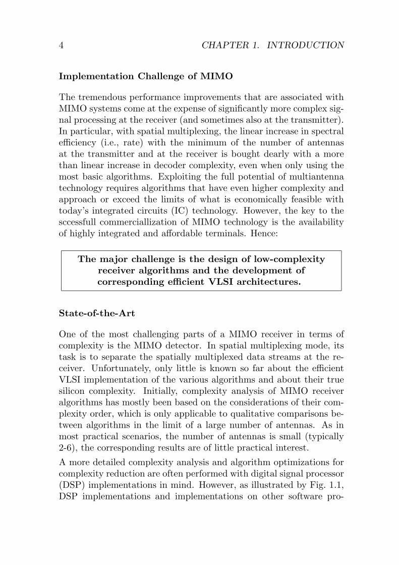
The tremendous performance improvements that are associated withMIMO systems come at the expense of significantly more complex sig-nal processing at the receiver (and sometimes also at the transmitter).In particular, with spatial multiplexing, the linear increase in spectralefficiency (i.e., rate) with the minimum of the number of antennasat the transmitter and at the receiver is bought dearly with a morethan linear increase in decoder complexity, even when only using themost basic algorithms. Exploiting the full potential of multiantennatechnology requires algorithms that have even higher complexity andapproach or exceed the limits of what is economically feasible withtoday’s integrated circuits (IC) technology. However, the key to thesccessfull commerciallization of MIMO technology is the availabilityof highly integrated and affordable terminals. Hence:
The major challenge is the design of low-complexityreceiver algorithms and the development ofcorresponding efficient VLSI architectures.
State-of-the-Art
One of the most challenging parts of a MIMO receiver in terms ofcomplexity is the MIMO detector. In spatial multiplexing mode, itstask is to separate the spatially multiplexed data streams at the re-ceiver. Unfortunately, only little is known so far about the efficientVLSI implementation of the various algorithms and about their truesilicon complexity. Initially, complexity analysis of MIMO receiveralgorithms has mostly been based on the considerations of their com-plexity order, which is only applicable to qualitative comparisons be-tween algorithms in the limit of a large number of antennas. As inmost practical scenarios, the number of antennas is small (typically2-6), the corresponding results are of little practical interest.
A more detailed complexity analysis and algorithm optimizations forcomplexity reduction are often performed with digital signal processor(DSP) implementations in mind. However, as illustrated by Fig. 1.1,DSP implementations and implementations on other software pro-

1.1. MIMO TECHNOLOGY 5
1M
100K
10K
1K
100
10
11 10 100 1K 10K 100K 1M 10M 100M 1G 10G
Com
puta
tionaleffort
per
data
item
[opera
tions/s
am
ple
]
New
arch
itectur
es
Low complexityalgorithms
High performancemicroprocessor
digitalsignal processor
dedicatedVLSI architectures
bit or symbol rate
1M
ops
1G
ops
1Tops
Figure 1.1: Examples for processing requirements of MIMO algo-rithms and processing capabilities of different hardware architectures.
grammable processing architectures can usually not meet the require-ments (in terms of throughput) of currently emerging and future wide-band MIMO systems. Consequently, dedicated VLSI architectures arestill needed for the implementation of the computationally most com-plex algorithms. Unfortunately, due to the considerable differencesbetween DSPs and dedicated VLSI circuits, the corresponding com-plexity estimates do not accurately reflect the true silicon complexityof an optimized VLSI implementation. For the same reason, someallegedly low-complexity schemes that were optimized for softwareimplementations even turn out to be ill-suited for ASIC implementa-tions.
Actual VLSI implementations of MIMO algorithms and of completeMIMO systems have only emerged recently. The few presented al-gorithms and designs provide initial reference points for the siliconcomplexity of MIMO detectors and illustrate suitable hardware ar-chitectures. Nevertheless, high-throughput wideband MIMO systemsrequire further improvements and optimizations to ensure that sys-tem performance is ultimately only limited by the wireless channel

6 CHAPTER 1. INTRODUCTION
capacity and not by the available receiver technology. Moreover, acomprehensive comparison of the true silicon complexity of differentdetection schemes and the associated performance tradeoffs and VLSIarchitectures based on actual VLSI implementations is so far onlyavailable in [5].
1.2. CONTRIBUTIONS 7
1.2 Contributions
The goal of this thesis is to explore the design space that is available onthe algorithmic and architectural level for the ASIC implementation oflow-complexity hard-decision MIMO detection for spatial multiplex-ing: For this purpose, algorithms have been optimized for hardwareimplementation and corresponding dedicated VLSI architectures havebeen developed. The associated implementation results provide refer-ence for the true silicon complexity of different MIMO receivers. Thedetailed contributions of this work to the efficient implementation ofthe different classes of MIMO detectors are as follows:
Linear and Successive Interference Cancellation (SIC) De-tection: Different implementation strategies are compared andit is shown that, with a proper implementation strategy, thebetter performing SIC algorithms are sometimes less costly toimplement (in terms of silicon area) than fully linear detectors.Moreover, an efficient scalable architecture is presented for lin-ear detection in MIMO-OFDM systems which achieves closeto 100% hardware utilization, low decoding latency, and highthroughput [6, 7].
In addition to linear and SIC detection, different methods formatrix inversion and matrix decomposition are considered. Thecomplexities of the available algorithms are analyzed and com-pared and suitable VLSI architectures are presented. In particu-lar different architectural and circuit-level tradeoffs are discussedfor the implementation of QR decomposition. The described ar-chitectures offer a wide range of tradeoffs between silicon areaand preprocessing latency.
Exhaustive Search Maximum Likelihood: It is shown how thisalgorithm which achieves optimum bit error rate performance,but with a complexity that grows exponentially in rate, canstill be implemented economically for rates that are surprisinglyhigh [8]. The reasons for this are a number of lossless1 algebraictransformations and an optimized VLSI architecture.
1in terms of bit error rate performance

8 CHAPTER 1. INTRODUCTION
Iterative tree-search algorithms: In this thesis, Sphere Decodingand K-Best decoding are subsumed under the framework of tree-search algorithms, which also comprises a number of other – lesswell known – search strategies.
With respect to the implementation of Sphere Decoding (SD)an efficient one-node-per-cycle VLSI architecture is presented[9] and it is shown how the algorithm can operate directly oncomplex-valued constellation points without the use of costlytranscendental functions [10]. Moreover, a new modified-normalgorithm is introduced [11] which reduces complexity on algo-rithm and on circuit level. In addition to that, a solution tothe problem of achieving a guaranteed minimum, but still highthroughput with SD is presented and it is explained how SD canbe pipelined.
With respect to the implementation of the K-Best algorithm, aVLSI architecture is described which, for a 4 × 4 system with16-QAM modulation, achieves a throughput that is eight timeshigher compared to the fastest circuit reported in the literature,while the area is almost the same [12]. On the theoretical side itis explained why the real-valued decomposition, which is foundto be unfavorable for Sphere Decoding, should be preferred forthe implementation of a K-Best decoder.
In summary, this work provides novel low-complexity solutions (al-gorithms and VLSI architectures) for the implementation of MIMOdetection. The described reference designs illustrate the performanceof the proposed methods and provide results for the true silicon com-plexity of corresponding implementations. To the best of our knowl-edge, all presented circuits are currently ranked among the highestperforming implementations of MIMO detectors reported in the openliterature.

1.3. OUTLINE OF THE THESIS 9
1.3 Outline of the Thesis
Chapter 2 describes the MIMO system model and discusses an im-portant system-level aspect which governs the partitioning of MIMOdetection algorithms into channel-rate preprocessing and symbol-ratedetection. The chapter also lists the performance criteria which con-stitute the basis for the development and evaluation of algorithms andVLSI architectures and introduces the available algorithm choices forMIMO detection, together with their corresponding complexity scal-ing behavior.In Chapter 3, the focus is initially on the implementation of linear de-tection and successive interference cancellation (SIC) algorithms andon the corresponding complexity/performance tradeoffs in the symbol-rate detection stage. The second part of the chapter is then concernedwith the implementation of matrix decomposition and matrix inver-sion algorithms, which are required for linear and SIC detection, aswell as for the tree-search algorithms which are described later inChapter 5.Chapter 4 deals with the implementation of maximum likelihood (ML)algorithms by means of an exhaustive search. It is shown how, de-spite the exponential complexity increase with the transmission rate,a suitable high-level architecture and algorithm optimizations enableefficient implementations of the scheme for rates that are surprisinglyhigh.Chapter 5 is dedicated to the implementation of iterative tree-searchalgorithms, which achieve full or close-to ML performance with re-duced silicon complexity. This class of algorithms includes SphereDecoding and K-Best decoding. The chapter starts with a descriptionof the basic concept behind the application of tree-search algorithmsto MIMO detection and with an explanation of how Sphere Decodingand K-Best decoding fit into this framework. The second and thirdparts of this chapter then focus on the two algorithms individually.They describe a number of algorithmic optimizations and correspond-ing VLSI architectures for their efficient implementation in silicon.Conclusions are drawn in Chapter 6.


Chapter 2
Preliminaries
The first part of this chapter provides a description of the MIMO sys-tem under consideration and introduces the notation and terms thatwill be used throughout this thesis. A brief review then introducesthe fundamental algorithm choices for MIMO detection which will bethe subject of the discussion in the subsequent chapters.
2.1 System Model
We start by noting that with proper modulation techniques such asOFDM or with proper equalization for example in CDMA most wide-band MIMO communication systems can be reduced to a set of nar-rowband MIMO systems. A narrowband system model can thereforebe considered as a simple canonical form based on which it is straight-forward to derive corresponding receivers for wideband MIMO com-munication systems. Hence, a simple narrowband system model shallserve as the basis for the subsequent discussions to ensure that theresults are applicable to a wide range of communication scenarios andto provide a common basis for the comparison of different algorithms.In the system under consideration, as depicted in Fig. 2.1, the numberof transmit antennas is given by MT and the number of receive an-tennas is given by MR. Because in this thesis we are only concerned
11

12 CHAPTER 2. PRELIMINARIES
with spatial multiplexing, we also assume MR ≥MT .
Transmitter: With spatial multiplexing, the modulation in the trans-mitter corresponds to choosing the entries of the transmitted signalvector s independently from a set of constellation points O, accordingto the data to be transmitted, so that s ∈ OMT . The set O is definedby the modulation scheme for which a rectangular QAM modulationwith Q = |O| bits per complex-valued scalar symbol and with Grayencoding is usually assumed. The rate of the corresponding MIMOsystem with MT transmit antennas in spatial multiplexing mode isthen given by R = MT log2 Q bits per channel use (bpcu). In thiswork the corresponding constellation points are defined on an odd in-teger grid according to O = {(1 + 2a) + j(1 + 2b)} with a, b ∈ Z asshown in Fig. 2.2. For a fair comparison which is independent of thenumber of transmit antennas and of the modulation scheme, the sig-nal vector s is normalized before transmission in such a way that theaverage transmitted power is one (i.e., E{‖s‖2} = 1).
MIMO Channel: The equivalent baseband model of the MIMOwireless channel that yields the MR-dimensional received vector y isgiven by the following input-output relation
y = Hs+ n. (2.1)
The MR-dimensional vector n models the thermal noise as indepen-dent identically distributed (i.i.d.) circular symmetric (proper) com-plex Gaussian with zero mean and variance σ2 per complex dimension(E{nnH} = σ2I). The MR ×MT dimensional matrix H representsthe complex-valued channel gains between each transmit and eachreceive antenna. For the simulations in the following chapters, ani.i.d. Rayleigh fading channel model (without correlation) is assumed.Hence, the entries of H are chosen independently as zero mean propercomplex Gaussian random variables with variance one per complexdimension. The SNR is defined in accordance with [4] as the ratiobetween the total transmitted power, which has been normalized toone, and the variance of the thermal noise according to
SNR = 1/σ2, (2.2)

2.1. SYSTEM MODEL 13
MIM
OD
etec
tor
sC
hann
el E
stim
atio
n
s
HS
/PP
/S
y
Figure 2.1: Block diagram of a MIMO communication system.

14 CHAPTER 2. PRELIMINARIES
1
1
-1
-1
13
13
-1 -3
-1-3
13
57
1357
-1 -3 -5 -7
-1-3
-5-7
4-Q
AM
(QP
SK
)
16-Q
AM
64-Q
AM
Figure 2.2: Constellation points for 4-QAM (QPSK), 16-QAM and64-QAM modulation.

2.1. SYSTEM MODEL 15
Receiver: The MR antennas at the receiver pick up the receivedsignal vector y. Taking into account that also the variance of thechannel gains have unit variance, the average received signal-to-noiseratio (over channel realizations) per receive antenna is immediatelygiven by the SNR.The task of the MIMO detector at the receiver is to obtain the bestpossible estimate of the transmitted signal vector s based on the re-ceived vector y. Coherent modulation (which is assumed in this thesis)also requires that the receiver is provided with an estimate H of thechannel H. Such an estimate can for example be obtained during aseparate training phase.

16 CHAPTER 2. PRELIMINARIES
2.2 System Level Considerations
The boundary conditions for the implementation of MIMO detectionare defined by the underlying communication system. Hence, it isimportant to take system level aspects into account. A particularlyimportant aspect arises from the observation that most MIMO re-ceiver algorithms can be partitioned into channel-rate and symbol-rateprocessing as illustrated in Fig. 2.3.
� Channel-rate processing is often also referred to as preprocessing.The term comprises all operations that need to be carried outonly when the channel estimate changes.
� Symbol-rate processing comprises all those operations that needto be carried out for each received symbol in order to estimatethe transmitted vector symbol. We shall refer to this part of thereceiver as the detection unit.
In practice, the channel can often be assumed to be constant overa large number of received symbols, so that channel-rate process-ing is less critical. This assumption may, however, no longer holdin high-mobility scenarios, under stringent latency constraints, or inwide-band MIMO systems with frequency selective fading. Still it isjustified, to consider the channel-rate processing complexity separatefrom the symbol-rate processing, as the frequency of the operation andthe performance requirements are dictated by a completely differentset of system parameters.
Channel ratepreprocessing
H
y
Symbol ratedetection
s
Figure 2.3: High-level block diagram of MIMO detection with separatepreprocessing and detection units.

2.3. DESIGN SPACE EXPLORATION 17
2.3 Design Space Exploration
Once the system level aspects and requirements are understood, onecan start with the development of low-complexity1 MIMO receivers.The available design space is comprised of a variety of algorithmschoices each of which provides opportunities for further optimizationson both algorithm and VLSI architecture level. At the same time,these choices and optimizations often entail tradeoffs between siliconarea, throughput and BER performance which need to be balancedby the designer. Hence, joint consideration of both algorithm and im-plementation aspects is crucial for achieving efficient, low-complexityimplementations.
BER Performance
The quality of a MIMO detection algorithm and of its associated im-plementation can be assessed by its BER performance which is ob-tained from computer simulations as corresponding analytical expres-sions are often not available or do not include nonidealities causedby implementation tradeoffs. In the following, we shall briefly definethe criteria that we use to describe and compare the BER perfor-mance characteristics of algorithms in a fading environment and ofcorresponding implementations:
Diversity Gain: Diversity gain describes the behavior of an algo-rithm in the limit of high SNR, and the diversity order correspondsdirectly to the slope of the BER curve. The uncoded spatial multi-plexing system (without transmit channel knowledge) considered inthis thesis can achieve a maximum diversity order of MR with anoptimum ML receiver.
SNR Penalty: The SNR penalty describes the difference in SNRthat is required by two algorithms to achieve the same target BER.Clearly, when algorithms exhibit different diversity orders, the SNR
1The term“low complexity” refers to minimizing area utilization while meetingcertain design targets in terms of throughput or delay.

18 CHAPTER 2. PRELIMINARIES
penalty increases at high SNR. For algorithms that exhibit the samediversity order, the SNR penalty translates into a shift of the BERcurve towards higher SNR.
Error Floor: In practical systems, the additive thermal noise termn in the channel model in (2.1) does not accurately model the over-all noise in an end-to-end system. Instead, other noise sources whosepower does not degrade with increasing SNR (according to the defini-tion in (2.2)) also contribute to the effective overall noise power. Athigh SNR, these constant terms become the dominant factors and theBER curve shows an error floor. In the systems under consideration inthis thesis, we will encounter error floors only due to implementationloss, caused by limitations on the dynamic range of variables and byquantization noise. In that case, proper design must ensure that thecontribution of the implementation loss is small compared to the ther-mal noise for the entire SNR operating range of the system. In otherwords, the error floor must be well below the BER performance that isachieved by the system under consideration under realistic operatingconditions.
Discussion of the Simulation Methodology:
As mentioned previously, the BER results in this thesis have been ob-tained from computer simulations based on the i.i.d. channel modeldescribed in Sec. 2.1. This model is valid in rich scattering environ-ments with sufficient spacing between the antennas (on the order ofone wavelength). In other scenarios, where the entries of the channelmatrix are correlated, simulation results need to be revisited and it isexpected that in particular the performance of linear and SIC detec-tors will be degraded. It is further noted that all presented simulationresults assume perfect channel knowledge at the receiver, effectivelysetting H = H, so that channel estimation and detection can be sep-arated.Most of the BER results are for a 4×4 MIMO system with 16-QAMmodulation. Clearly, the corresponding performance charts repre-sent only a snapshot of the wide range of possible antenna configura-tions and modulation schemes. The main motivation behind choosing

2.3. DESIGN SPACE EXPLORATION 19
MT = 4 is the fact that four antennas already provide a consider-able capacity improvement that is likely to cover the needs for nextgeneration wireless systems. Moreover, from a practical perspective,mounting more than four antennas with an appropriate distance (ap-proximately one wavelength apart) on a portable device appears dif-ficult2. For the same reason, the BER performance of asymmetricsetups (MR > MT ) has not been investigated explicitly in this work,even though such system configurations would help to close the per-formance gap between ML and suboptimal receiver algorithms [4]. Onthe other hand, MIMO systems with MT = 2 and MR=2–4 are cer-tainly a relevant case. However, the implementation of correspondingreceiver algorithms (for two spatial streams) does not constitute amajor research challenge.
In terms of the modulation scheme, 16-QAM has been chosen as a rep-resentative case. Nevertheless, it is important to noted that practicalsystems will employ adaptive modulation, predominantly using QPSKto 16-QAM for outdoor scenarios and QPSK to 64-QAM for indoorscenarios [13]. First order estimate of the BER performance for mod-ulation schemes not shown in this thesis can be obtained by simplyshifting the reported results by 7 dB to the left for QPSK and 6.5 dBto the right for 64-QAM. The reason for this straightforward transfor-mation is that the BER performance is a function of SNRd2min, wheredmin is the minimum distance between constellation points. Hence,the reduction of d2min that is associated with higher-order modulationschemes can be translated into an SNR shift. An exception are simu-lations concerning the implementation loss due to fixed-point effects.Here, error floors arise from quantization noise. Consequently, whenhigher order modulations are considered, the SNR operating range,given by the error floor with a particular modulation scheme, remainsthe same for all other modulation schemes and the corresponding errorfloors must be adjusted accordingly.
2Note that for example all IEEE 802.11n standard proposals only consider upto four antennas.

20 CHAPTER 2. PRELIMINARIES
Design Criteria and Complexity Analysis
The complexity of an algorithm can be estimated at different levels ofabstraction. However, no generally applicable methodology exists thatis capable of accurately predicting the final VLSI implementation com-plexity and performance of a fundamental signal processing scheme asa function of a high-level description of the algorithm. The reason forthis dilemma is the large design space that is associated with algo-rithm optimizations for complexity reduction, with the implicationsof fixed-point considerations and with the development of optimizedVLSI architectures. Moreover, the vast disparity between processingtechnologies (such as DSPs, FPGAs, and ASICs) often precludes atransfer of complexity estimates or of optimizations for complexityreduction of an algorithms from one technology to another. Hence,taking an algorithm all the way to its final implementation in a specifictechnology is often the only way to obtain reliable estimates of its trueimplementation complexity. However, taking an algorithm all the wayto a final implementation is extremely time consuming. Therefore, ahierarchical design process must be employed to estimate complexitywith increasing precision at different levels of abstraction throughoutthe design process.
Complexity Order: The complexity order of an algorithm providesdescription of the scaling behavior of its complexity in one or multipledesign parameters in the limit of infinity. A complexity order of O(n2)for example specifies that the fastest growing term in the expressionfor the corresponding complexity is quadratic in n. Unfortunately,the complexity order does not allow for a direct comparison betweenalgorithms, as all lower order terms (which are most relevant in manypractical scenarios) are not taken into account.
Computational Complexity: The computational complexity de-scribes the complexity of an algorithm in terms of number of costlyoperations. However, in practice, the notion of what kind of oper-ation qualifies as costly differs widely depending on the underlyingimplementation technology. For floating-point DSP implementationsfor example, multiplications and additions generally entail comparable

2.3. DESIGN SPACE EXPLORATION 21
execution times and only rarely occurring complex operations such asdivisions and transcendental functions have longer (but still often com-parable) execution times. Hence, the bare number of floating-pointoperations is therefore often a viable initial estimate of the complexityof an algorithm.In dedicated fixed-point VLSI implementations, complexity heavilydepends on the type of operation and on the associated fixed-pointprecision requirements. Moreover, as opposed to DSP implementa-tions, VLSI implementations allow for replacing sequences of basicoperations by much more efficient single-cycle custom composite op-erations and additional hardware resources can be allocated for par-allel execution of more frequent or more time consuming operations.Hence, a measure for complexity that simply counts all kinds of basicarithmetic operations equally and independently is usually misleadingand provides a poor estimate of the VLSI implementation complexity.Thus, it is important to identify the complexity defining operationswith a basic VLSI architecture in mind and to count the associatedefforts individually. Such careful counting of operations (with a VLSIarchitecture and the associated memory requirements in mind) pro-vides a reasonable means for the comparison of similar algorithmswhich call for similar underlying architectures and for assessing theimpact of corresponding optimizations. Hence, we shall follow thisstrategy (which obviously requires iterations between algorithm op-timizations and VLSI architecture development) throughout the re-mains of this thesis.
True (Silicon) Complexity: Unfortunately, even smart ways ofcounting the number of operations tend to fail, when comparing fun-damentally different algorithms or when attempting to accurately pre-dict the capabilities of a final VLSI implementation. Moreover, count-ing of operations does not immediately provide information about thedesign tradeoffs between throughput and silicon area, as data depen-dencies, memory access bottlenecks and other potential impairmentsare not captured.The true silicon (or implementation) complexity of an algorithm isgiven by the area and the throughput or delay that is achieved witha particular VLSI architecture. The word “true” thereby alludes to

22 CHAPTER 2. PRELIMINARIES
the fact that the corresponding results are based on actual implemen-tations of the algorithm. The drawback of that measure is that theimplemented architectures only provide reference points in the designspace for a specific set of design parameters (e.g., number of anten-nas, modulation schemes or throughput requirements), which may noteven represent the best possible solution. However, with a thoroughunderstanding of the underlying architectures, such reference pointsdo provide a solid basis to derive realistic estimates for the true siliconcomplexity of designs with other design parameters.
2.4 MIMO Detection Schemes
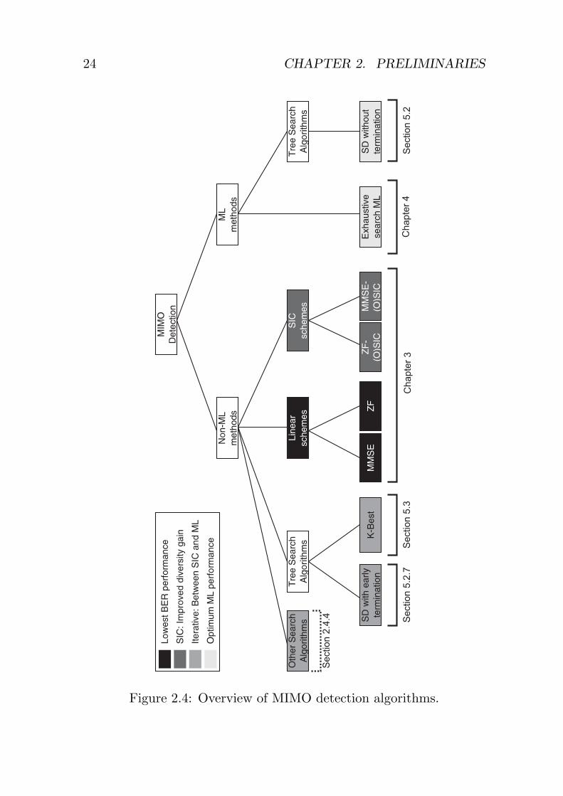
Let us start by briefly reviewing the different classes of MIMO de-tectors and their associated BER performance and complexity scalingbehavior. In particular, we limit our discussion in this thesis to theproblem of solving (2.1) without including a subsequent channel de-coder. Hence, maximum likelihood sequence estimation algorithms,such as the Viterbi algorithm, are not part of our considerations be-cause they are not immediately applicable to (2.1). Instead, we assumebit-interleaved-coded-modulation [14], where, after proper interleav-ing, the output of the described MIMO detectors constitutes the inputto a subsequent channel decoder.
Among the available schemes for MIMO detection, one can identifyfour main categories based on the underlying strategy that is used tosearch for the corresponding estimate of the transmitted signal vector:
� Linear and successive interference cancellation (SIC) detection
� Exhaustive search maximum likelihood detection
� Iterative tree search algorithms
� Other iterative search algorithms
In the following, only implementations for algorithms of the first threeclasses will be presented, while only a short summary of the basic ideabehind algorithms of the fourth kind is given in Sec. 2.4.4. An overview
2.4. MIMO DETECTION SCHEMES 23
of the most prominent schemes under consideration and their affili-ations to the above categories is given in Fig. 2.4. In the chart, wedistinguish between ML and non-ML algorithms whereby the colorsprovide a further initial indication about the achievable BER perfor-mance, mainly based on the ability of the decoders to exploit thediversity in the MIMO channel. A more quantitative performanceevaluation is provided by the simulation results, shown in Fig. 2.5 fora 4×4 system with 16-QAM modulation.
2.4.1 Linear and SIC Detection
Linear Detection
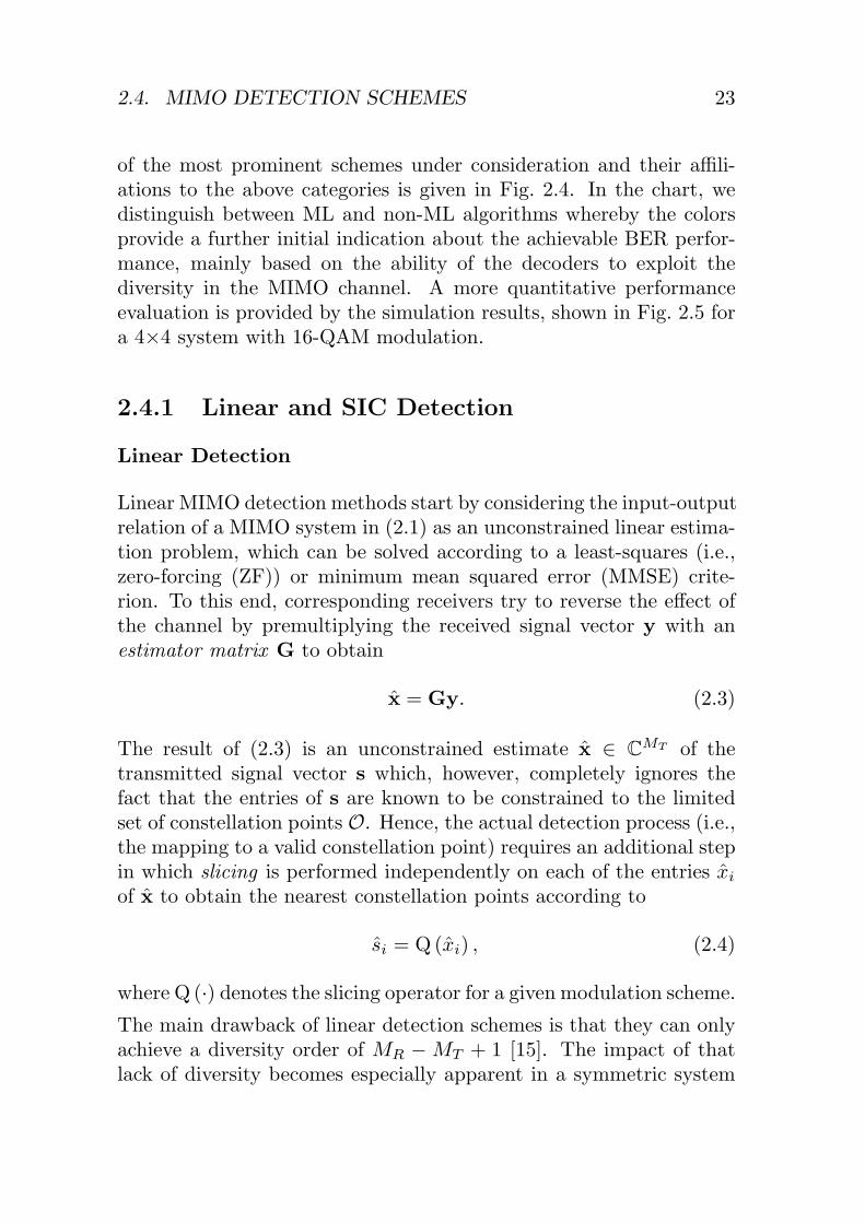
Linear MIMO detection methods start by considering the input-outputrelation of a MIMO system in (2.1) as an unconstrained linear estima-tion problem, which can be solved according to a least-squares (i.e.,zero-forcing (ZF)) or minimum mean squared error (MMSE) crite-rion. To this end, corresponding receivers try to reverse the effect ofthe channel by premultiplying the received signal vector y with anestimator matrix G to obtain
x = Gy. (2.3)
The result of (2.3) is an unconstrained estimate x ∈ CMT of the
transmitted signal vector s which, however, completely ignores thefact that the entries of s are known to be constrained to the limitedset of constellation points O. Hence, the actual detection process (i.e.,the mapping to a valid constellation point) requires an additional stepin which slicing is performed independently on each of the entries xi
of x to obtain the nearest constellation points according to
si = Q(xi) , (2.4)
where Q (·) denotes the slicing operator for a given modulation scheme.The main drawback of linear detection schemes is that they can onlyachieve a diversity order of MR −MT + 1 [15]. The impact of thatlack of diversity becomes especially apparent in a symmetric system
24 CHAPTER 2. PRELIMINARIES
Section
2.4
.4 Section
5.2
.7S
ection
5.3
Chapte
r3
Chapte
r4
Section
5.2
Figure 2.4: Overview of MIMO detection algorithms.

2.4. MIMO DETECTION SCHEMES 25
Figure 2.5: BER performance comparison of ZF, MMSE, SIC,V-BLAST and ML in a 4×4 system with 16-QAM modulation (50’000channel realizations).
configuration with MT = MR. The corresponding poor BER per-formance at high SNR is clearly visible in the simulation results inFig. 2.5.
In terms of complexity, channel-rate preprocessing for linear detectioncalls for matrix decomposition or matrix inversion. Such algorithmsare associated with a complexity order that is roughly O(MRM2
T )3.
Strictly speaking, the complexity order of the symbol-rate detection isgiven by the slicing operation, which is exponential in the order of the
3While matrix inversion is generally assumed to have cubic complexity order,advanced algorithms with lower complexity order have been developed [16]. How-ever these are rarely relevant in practice and are not considered here.

26 CHAPTER 2. PRELIMINARIES
employed modulation scheme. However, due to the simplicity of theslicing operation and due to the fact that very high order modulationschemes are rarely used because of poor BER performance, slicingcan be neglected in practice. Hence, the complexity of the detectionis dominated by a matrix-vector multiplication in (2.3) or by backsubstitution, which may be performed instead. Both operations havea complexity order that scales with the number of transmit and receiveantennas according to O(MRMT ).
Zero Forcing (ZF) Detection: ZF detection aims at a perfectseparation of the parallel data streams. To this end, the least-squaresestimator G is obtained as the Moore-Penrose pseudoinverse of thechannel matrix H as
G = (HHH)−1HH = H†. (2.5)
In the special case of MT = MR the Moore-Penrose pseudoinverse isidentical to the straightforward inverse of H, which may be obtainedimmediately with lower complexity as
G = H−1. (2.6)
The application of (2.5) or (2.6) to (2.3) yields
x = s+ nZF with nZF = Gn (2.7)
so that the effective channel H between the transmitter and the slicerat the receiver now corresponds to the identity matrix (H = I). Hence,the interference from all other parallel streams streams has been elim-inated completely as desired. However, the drawback of the ZF esti-mate is that perfect separation of the transmitted data streams entailsan enhancement of the additive noise, which is now given by nZF.
Biased MMSE Estimator: Instead of forcing the interference termsto zero, regardless of the noise, MMSE detection minimizes the overallexpected error by taking the presence of the noise into account. Fromestimation theory it can easily be shown that the optimum tradeoff

2.4. MIMO DETECTION SCHEMES 27
between interference cancellation and noise enhancement is achievedby setting
G = (HHH+MTσ2I)−1HH . (2.8)
After substituting (2.8) into the input-output relation of our MIMOsystem (2.3) we now obtain
x = Hs+ nMMSE with nMMSE = Gn, (2.9)
where H = GH is the effective channel after MMSE equalization. Asopposed to the ZF case, the off-diagonal elements of H are no longerzero, which leads to the expected residual interference. However, theMMSE estimator is also a biased estimator which causes the diagonalentries of the effective channel to be smaller than one (Hi,i < 1). Theresult is a shrinkage of the constellation after MMSE equalizationcompared to O. While the bias has no impact on constant-modulusmodulation schemes (e.g., QPSK or 8-PSK), it is expected to entailsa marginal BER performance degradation for non constant-modulusmodulation schemes such as 16-QAM or 64-QAM.
Unbiased MMSE Estimator: According to [17], the unbiasedMMSE estimator G can be obtained from the biased estimator Gby scaling its rows with the corresponding reciprocal diagonal entriesof the resulting effective channel H according to
G = diag(1
h11, . . . ,
1hMT MT
)G, (2.10)
where the operator diag (·) constructs the corresponding diagonal ma-trix. An alternative approach which avoids the computation of (2.10)is to keep the biased estimator G and to simply adapt the decisionboundaries of the slicing operation in (2.4) according to hi,i. However,unfortunately, both approaches still require the computation of hi,i,which has non-negligible computational complexity.For assessing the value of the additional complexity that is incurredby properly accounting for the bias, it will be useful to consider thecorresponding impact on BER performance by means of simulations.

28 CHAPTER 2. PRELIMINARIES
Figure 2.6: BER performance comparison of biased and unbiasedMMSE detection in a 4×4 system with 16-QAM and 64-QAM modu-lation (5’000 channel realizations).
Fig. 2.6 shows the results for a 4×4 MIMO system with 16-QAM and64-QAM modulation. Clearly, the performance improvement fromusing the unbiased MMSE detector is only marginal. In the case of16-QAM modulation, the SNR penalty with the unbiased estimator isbelow 0.4 dB, while for 64-QAM the penalty reduces further to below0.1 dB. Hence, we conclude that the additional effort for computingthe diagonal terms of H for removing the bias is in most cases notrequired and the unbiased estimator can be used instead.

2.4. MIMO DETECTION SCHEMES 29
Successive Interference Cancellation (SIC)
SIC is based on the previously described linear estimation algorithms.However, a nonlinear interference cancellation stage partially exploitsthe knowledge that the entries of the transmitted vector s have beenchosen from a finite set of constellation points O. To this end, thesymbols of the parallel data streams are no longer all detected at once.Instead, they are considered one after another and their contribution(after slicing and remodulation) is subtracted (removed) from the re-ceived vector before proceeding to detect the next stream.
Compared to linear detection schemes, SIC achieves an increase indiversity order with each iteration. While the first detected streamstill sees a diversity order of MR −MT + 1, the second has alreadya diversity order of MR −MT + 2 and so forth. Unfortunately, theoverall average BER performance is dominated by the stream that isdetected first and error propagation also has a considerable impacton the performance of the subsequent streams. Hence, the detectionorder is important for achieving good BER performance as illustratedin Fig. 2.7 which,for a 4×4 system with 16-QAM modulation, providesa comparison of SIC without ordering to SIC with different orderingschemes and to linear MMSE detection.In terms of complexity, it is expected that a certain complexity over-head, compared to linear detection schemes, will be associated withfinding a suitable detection order. However, with the exception of theoriginal (in terms of complexity suboptimal) V-BLAST algorithm [18],the channel-rate preprocessing for SIC detectors exhibits the samecomplexity order as linear detection schemes. For the symbol-ratedetection, remodulation and interference cancellation only leads to aconstant factor in terms of complexity so that also complexity order ofthe detection process remains unchanged compared to linear schemes.
Unordered SIC: For the mathematical description of the basic SICalgorithm without (i.e., with arbitrary) ordering we assume that thefirst stream is detected first, followed by the second, and so forth untilthe last. The algorithm starts by initializing y(1) = y and definesH(i) = [ hi hi+1 . . . hMT ], where hi denotes the i-th column ofH. The matrices G(i) denote the linear ZF or MMSE estimators that

30 CHAPTER 2. PRELIMINARIES
MMSE OSICs withcolumn-norm orderingMMSE OSICs withcolumn-norm ordering
Figure 2.7: BER performance comparison for SIC detection with dif-ferent ordering strategies in a 4×4 system with 16-QAM modulation(10’000 channel realizations).
correspond to H(i). Starting from i = 1, SIC now proceeds as followsuntil i =MT :
xi = G(i)i y(i) (2.11)
si = Q(xi) (2.12)
y(i+1) = y(i) − sihi (2.13)
The nulling vectors G(i)i for the i-th streams are simply given by the
i-th row of the corresponding G(i). As expected from the previousdiscussion and as illustrated by the simulation results in Fig. 2.7, theoverall diversity order of unordered SIC corresponds roughly to the

2.4. MIMO DETECTION SCHEMES 31
diversity order of the first stream which is given by MR −MT + 1.However, in terms of BER performance, the unordered SIC detectoralready shows a performance gain in terms of SNR of almost 1.4 dBover linear MMSE detection.
Ordered SIC Detection (OSIC): Ordering aims at reducing thelikelihood of detection errors by attempting to identify the stream thatare most likely to yield no detection errors in the first iterations. As-sume that a suitable detection order is a priori known and is describedby a permutation P of the natural detection order {1, 2, . . . ,MT }. Or-dered SIC then starts by rearranging the columns ofH according to P(Hj = H{P}j
), followed by SIC as described in Eq. 2.11–2.13. Finally,the entries of the decoded signal vector s need to be rearranged to re-store the original order (s{P}i
= si). In the following, we shall brieflyconsider two low-complexity ordering strategies and their impact onBER performance:The most simple ordering scheme assumes that the per-stream re-ceived SNR is a measure for how reliably it can be detected. Underthis heuristic assumption, and knowing that the thermal noise poweris the same for all streams the detection order P is defined basedon the squared �2-norms of the columns of H in such a way thatP{P}i
≥ P{P}i+1 , where Pj = ‖hj‖2. As can be seen from the chart inFig. 2.7 this simple ordering already improves the BER performancesignificantly compared to unordered SIC. The graph also shows thatapproximating the computationally complex squared �2-norm with themuch less complex �1- or �∞-norm does not entail a noticeable loss inBER performance.The second ordering strategy employs the sorted QR decompositionalgorithm described in [19] as preprocessing for SIC detection. Thecomplexity of that scheme is slightly higher than the column-norm or-dering. However, the algorithm achieves better BER performance (c.f.Fig. 2.7) and is only 1 dB away from SIC with the much more com-plex, but optimum V-BLAST ordering, which we shall briefly considernext.
V-BLAST Ordering: The V-BLAST algorithm [18] finds the or-dering which optimum with respect to BER performance when only
32 CHAPTER 2. PRELIMINARIES
the nature of the channel is taken into account. To this end, thealgorithm determines the order in such a way that the noise on xi
in (2.11) is minimized in each iteration and consequently, the errorprobability of the subsequent slicing operation is also minimized. Anordering which yields even better BER performance in combinationwith SIC can only be achieved by taking the actual noise realizationinto account, as recently demonstrated in [20].
With the original V-BLAST scheme in [18], preprocessing has a com-plexity order of O(MRM3
T ). However, the optimized algorithm in [21]arrives at the same ordering with a complexity order that is given byO(MRM2
T ), which corresponds to the complexity order of the prepro-cessing stage for linear MIMO detection.
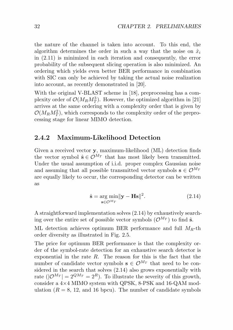
2.4.2 Maximum-Likelihood Detection
Given a received vector y, maximum-likelihood (ML) detection findsthe vector symbol s ∈ OMT that has most likely been transmitted.Under the usual assumption of i.i.d. proper complex Gaussian noiseand assuming that all possible transmitted vector symbols s ∈ OMT
are equally likely to occur, the corresponding detector can be writtenas
s = arg mins∈OMT
‖y −Hs‖2. (2.14)
A straightforward implementation solves (2.14) by exhaustively search-ing over the entire set of possible vector symbols (OMT ) to find s.
ML detection achieves optimum BER performance and full MR-thorder diversity as illustrated in Fig. 2.5.
The price for optimum BER performance is that the complexity or-der of the symbol-rate detection for an exhaustive search detector isexponential in the rate R. The reason for this is the fact that thenumber of candidate vector symbols s ∈ OMT that need to be con-sidered in the search that solves (2.14) also grows exponentially withrate (|OMT | = 2QMT = 2R). To illustrate the severity of this growth,consider a 4×4 MIMO system with QPSK, 8-PSK and 16-QAM mod-ulation (R = 8, 12, and 16 bpcu). The number of candidate symbols

2.4. MIMO DETECTION SCHEMES 33
to be considered for each received vector becomes 256, 4′096, and65′536, respectively.
2.4.3 Iterative Tree-Pruning Algorithms
Iterative tree-pruning algorithms are an attempt to achieve full orclose-to ML performance with a computational complexity that is (atleast on average) much lower than the complexity of an exhaustivesearch. The basic idea behind all algorithms of this kind is to startby transforming the original input-output relation in (2.1) in such away that one obtains a fully equivalent detection problem where thecounterpart of the channel matrix H is a triangular matrix R. Thisgoal can, for example, be achieved by first applying QR-decompositionto H, which yields a triangular matrix R and a unitary matrix Q sothat H = QR. Rotating the received vector y with QH then yields amodified input-output relation of the form
y = Rs+QHn with y = QHy. (2.15)
Before showing how to exploit this modified expression to reduce thecomplexity of the detection process, we introduce the set of noiselessreceived vector symbols which are defined by all possible incarnationsof z = Rs with s ∈ OMT . Thanks to the triangular structure ofR, one can now also define sets of noiseless partial received vectorsthrough z(i) =
[zi zi+1 . . . zMT
], whose entries depend only
on s(i) =[
si si+1 . . . sMT
]. One can associate the possible in-
carnations of z(i) with the nodes on the i-th level of a decision tree4,which has its root on level i = MT + 1 and whose leaves on leveli = 1 ultimately represent the set of all possible noiseless receivedvectors z(MT ) = z. Solving the ML detection problem now corre-sponds to iteratively searching this tree for the leaf whose associatedz lies closest to y. This search can be performed using a variety of low-complexity algorithms that employ different criteria and constraintsto quickly prune entire subtrees which are at least unlikely to con-tain the ML solution. The most prominent examples of tree-searchalgorithms for MIMO detection are Sphere Decoding (SD) and K-Best
4Note that | {z(i)} | = 2MT +1−i.

34 CHAPTER 2. PRELIMINARIES
decoding, which both have their origins in [22] and were introducedto wireless communications in [23] and [24], respectively. In the lit-erature, both algorithms are sometimes referred to as lattice-decodingtechniques [25]. However, as it will become clear from the discussionin Sec. 5, a lattice structure of the constellation points is not requiredfor leveraging considerable complexity savings.
Depending on the tree-pruning strategy, the corresponding algorithmsmay or may not always yield the ML solution. SD for example achievesfull ML performance if the search time of the decoder is not con-strained. K-Best decoding, on the other hand, resembles more animproved version of a SIC detector which cannot achieve ML perfor-mance.
From a complexity perspective, tree-search algorithms require a lin-ear preprocessing stage to perform the QR-decomposition which leadsto (2.15). The associated complexity order is the same as for lineardetection and is given by O(MRM2
T ). The computational complexityand even the complexity scaling behavior of the symbol-rate detectiondepend heavily on the employed tree-pruning algorithm. The instan-taneous decoding complexity of SD, for example, varies from symbolto symbol, depending on the geometry of the current channel realiza-tion, the noise realization, and the transmitted symbol. The averagecomputational complexity is a function of the SNR. With respect tothe scaling behavior, the order of the worst-case complexity of sequen-tial SD corresponds to an exhaustive search and is thus exponential inthe rate. For the average complexity, it was been found in [26, 27] thatthe complexity order is polynomial in the rate, while it is argued in[28, 29] that, in the limit of high rates, the scaling behavior of even theaverage complexity of SD is still exponential in the rate. As opposedto sequential SD, the K-Best algorithm has a fixed, implementationdependent computational complexity that depends on the number oftransmit antennas MT and on the design parameter K, whereby ahigher K generally results in a better BER performance. The associ-ated complexity order is given by O(M2
TK). However, in practice, Kmust be chosen as a function of the rate in order to maintain close-toML performance5. Hence, complexity also depends on the order of
5So far, no analytical results are available to predict a suitable K for a givenrate. Therefore, K must be chosen based on simulation results.

2.4. MIMO DETECTION SCHEMES 35
the modulation scheme and tends to grow faster than quadratically inMT .
2.4.4 General Search Algorithms
Besides the iterative tree-search algorithms, described in Sec. 2.4.3,other search algorithm with close-to ML performance but with non-exponential complexity order have recently been proposed. The fun-damental idea behind these concepts is to start by identifying a smallset of vector symbols which is likely to contain the ML estimate.A particularly promising idea to identify such a reduced set of can-didates is the notion of idealized bad channels (IBC) which has beenintroduced in [30]. These IBCs are characterized by having a sin-gle small eigenvalue which gives rise to a dominant noise componentalong the corresponding eigenvector after MMSE or ZF equalization.The Line-Search detector (LSD), described in [30] and [31], and theSphere-Projection algorithm (SPA), described in [30] and [32], usesthe notion of IBCs to identify a subset of candidate vector symbolsthat will be considered in the search for the constellation point thatends up closest to the received vector y. With respect to BER, bothdetectors get very close to ML performance. However, because theML solution may not be part of the reduced subset of vector symbolsa small performance penalty must be accepted.In terms of complexity, it is clear that both schemes considerablyreduce the number of candidate vector symbols, compared to an ex-haustive search. It has been found in [30] that the LSD exhibitsa complexity order of O(M3
TQ)6. The SPA has a complexity orderof O(M2
T
√Q). However, a closer consideration of the described al-
gorithm also shows that a considerable number of costly arithmeticoperations is required to identify this reduced set of candidates foreach received vector. As a result, the complexity of the symbol-rateprocessing will be high.
6The corresponding reference states O(M3T P ), where P is the number of de-
cision boundaries which grows according to O(√
Q), where Q is the order of themodulation scheme.


Chapter 3
Implementation ofLinear/SIC Detection
All linear and SIC algorithms that were introduced in Sec. 2.4.1 arebased on the same fundamental concepts of estimation theory andlinear algebra. It is thus not surprising that all of them share thesame complexity scaling behavior for both the channel rate and forthe symbol-rate processing. However, the detection schemes differwidely in their BER performance and in their computational complex-ity. Moreover, a considerable number of algorithm choices exist for theactual implementation of most of the described linear detection andSIC strategies. While most of these choices are fully equivalent froma BER performance perspective in a floating-point implementation,they exhibit significant differences in their computational complexi-ties, and in their numerical requirements, and thus ultimately also intheir true silicon complexity.
The first part of this chapter compares the different linear and SICalgorithms based on ZF and MMSE criteria with repect to their corre-sponding VLSI architectures and implementation complexities. Thesecond part is concerned with the algorithm choices for the imple-mentation of matrix inversion and matrix decomposition algorithmswhich constitute the basis for linear and SIC algorithms and for the
37

38 CHAPTER 3. LINEAR/SIC DETECTION
iterative tree-search algorithms, presented in Chap. 5. CorrespondingVLSI architectures and reference implementation results conclude thediscussion.
3.1 Detection Stage
With linear detection and SIC algorithms, the line between channel-rate preprocessing and symbol-rate detection can be drawn in twodifferent places, leading to significant differences in the algorithmsthat must be employed for the final implementation. The first methodis referred to as matrix-multiplication (MM) based detection, and thesecond approach as back-substitution (BS) based detection.
3.1.1 Matrix-Multiplication Based Detection
The first approach for implementing the symbol-rate detection strictlyfollows the description in Sec. 2.4.1, where the nulling vectors (Gi
or G(i)i ) are directly applied to the received vector y. The corre-
sponding computational complexity amounts toMTMR full1 complex-valued multiplications, which can be implemented using a wide rangeof area/delay tradeoffs that are available from resource sharing andparallel processing.
Linear Detection: An example for the VLSI architecture of a lineardetection unit that computes s inMR clock cycles is shown in Fig. 3.1.The numbers in the arithmetic units represent estimates of their arearequirements. The reason for the considerable area of the multiplieris that the nulling vectors must be represented with a considerablenumber of bits to cover a large dynamic range and to provide sufficientaccuracy in a fixed-point implementation. Finally, in addition to thearea for the detector, linear detection also requires MTMR words ofmemory to store the nulling vectors.
1The term “full” is used to refer to arithmetic units, mainly multipliers, inwhich all operands are variable and involve a considerable number of bits.

3.1. DETECTION STAGE 39
yj
G1,j
G2,j
GMT ,j
300 GE4K GE
Gi,j
yj sj
sj
sj
sMT
MAC
16
8x16 Bit16
8 16
192 GE
Figure 3.1: Block diagram of a matrix-multiplication based lineardetector.
SIC Detection: The step from linear detection to SIC mainly in-volves supplementing the multiply-accumulate (MAC) operation thatapplies a nulling vector with a subsequent interference cancellationstage as shown in Fig. 3.2. As the additional multipliers can be re-duced to few adders and multiplexers [33, 34, 35] because one of theirinputs is only chosen from the small set of constellation points, theadditional area overhead is comparatively small. Throughput can beincreased by instantiating multiple (extended) MAC units. However,as opposed to the linear detector, where all MAC units can operatein parallel, they must be cascaded for the SIC detector as illustratedin Fig. 3.2. In terms of memory requirements, SIC requires boththe nulling vectors G and the channel coefficients H. Hence stor-age requirements are doubled to 2MTMR words compared to lineardetection.
3.1.2 Back-Substitution Based Detection
The BS algorithm solves linear systems of equations of the form
y = Rs, (3.1)

40 CHAPTER 3. LINEAR/SIC DETECTION
300 GE6K GE
1K GE
300 GE
Feedback for a single detection unit
yj
yj
G1,j Hj,1
s1 s2 sMT
G2,j Hj,2 GMT ,j Hj,MT
Gi,j Hj,i
MR
si
i = 1 i = 2 i = MT
16
12
12
16
144 GE
16
144 GE
192 GE
Figure 3.2: Block diagram of matrix-multiplication based SIC detec-tion.
under the condition that the matrixR is upper2 triangular. By settingy = Θy and by computing Θ and R in the preprocessing in such away that R−1Θ = G, BS can be applied directly in the detectionstage of a linear or SIC detector.
Linear Detection: For a linear receiver, (3.1) must then be solvedas an unconstrained detection problem. To this end, the followingiteration is carried out for i =MT , . . . , 1 after initializing y(MT ) = y:
xi =1
Ri,iyi (3.2)
y(i−1) = y(i)i−1 − rixi, (3.3)
where the term 1/Ri,i in (3.2) is usually precomputed once so thatcomputing xi requires only a multiplication. The vectors y
(i)i−1 and ri
2Exactly the same considerations apply also to lower triangular matrices. How-ever for clarity of explanation we shall only consider the upper triangular formthroughout the rest of this thesis

3.1. DETECTION STAGE 41
thereby denote the first i− 1 entries of y(i) and of the correspondingentries of the i-th column of R, respectively. The associated computa-tional complexity amounts to MTMR complex-valued multiplicationsfor computing y, for example by using a circuit as the one shown inFig. 3.13 and toMT (MT+1)/2 complex-valued multiplications for theiteration that carries out the BS in (3.2) and (3.3). As opposed to theMM-based detection scheme, slightly more memory storage is requiredto keep the MT (MT + 2MR + 1)/2 entries4 of Θ and R. We shall seelater, how Θ and R can be obtained directly from the channel matrixH during preprocessing, without the need to explicitly compute thelinear estimator G.In terms of its suitability for VLSI implementation, the BS algorithmsuffers from its data dependencies, which limit the amount of parallelprocessing and lead to a poor resource utilization in parallel VLSIarchitectures. A 100% resource utilization can only be achieved in afully decomposed architecture, such as the one in Fig. 3.3(a), whichcarries out the BS part of a linear receiver in MT (MT + 1)/2 cycles.Again, a considerable part of the overall complexity of the circuitmust be attributed to the complex-valued multiplier, which needs alarge dynamic range mainly because of the precomputed normalizationcoefficient 1/Ri,i in (3.2).
SIC Detection: In order to adapt the BS-based linear detectionstage to perform SIC, a slicing operation is introduced into (3.2) toobtain the following iteration:
xi =1
Ri,iyi (3.4)
si = Q(xi) (3.5)
y(i−1) = y(i)i−1 − risi. (3.6)
In the above algorithm, the full complex-valued multiplications in (3.3)now merely correspond to multiplications with constellation points.
3Because the matrix Θ is unitary, the width of the multiplier in Fig. 3.1 canbe reduced to say 8× 8 bit, which reduces its silicon area from 4K GE to 2K GE.
4Note that the fact that some entries are only real-valued is ignored here inorder to keep the complexity estimate simple. Compared to the overall complexity,the impact of this slightly pessimistic estimate is small.

42 CHAPTER 3. LINEAR/SIC DETECTION
7K GERi,j
yj
sj
300 GE
a)
MT
−1
1/Ri,i
<1K GE
Ri,j
yj
sj
300 GE
b)
MT
−1
Ri,i
FIFOFIFO
600 GE16x16 Bit 16
12
8
12
Figure 3.3: Block diagram of BS-based linear detection (left) and SICdetection (right).
The only remaining costly operations are the multiplication in (3.4)and the division that is required to compute 1/Ri,i in the prepro-cessing. However, both operations can be avoided by absorbing thecorresponding normalization into the slicing operation in (3.5), whereonly the decision boundaries can be adjusted according to Ri,i. Thereduced-complexity iteration for back-substitution then proceeds asfollows, without the need for costly full complex-valued multiplica-tions:
si = Q(yi, Ri,i) (3.7)
y(i−1) = y(i)i−1 − risi. (3.8)
The computational complexity now amounts to onlyMTMR full complex-valued multiplications for the computation of y, as for the linear SICdetection and to MT (MT + 1)/2 reduced-complexity multiplicationsfor the BS process. The block diagram of a fully decomposed VLSIarchitecture for carrying out the BS for SIC is shown in Fig. 3.3(b).The circuit is similar to the one for linear detection with BS. However,the complex multiplier has been replaced by a significantly smaller op-timized multiplier.

3.1. DETECTION STAGE 43
3.1.3 Slicing
The slicing operation is first considered for the simple case of MM-based linear detection and SIC as well as for BS-based linear detec-tion. All three methods yield a properly normalized xi. Hence, withthe constellation points on an odd integer grid, as defined in Sec. 2.1,slicing of xi simply corresponds to computing int ((�{xi}+ 1) /2) andint ((�{xi}+ 1) /2), where int (·) denotes rounding to the nearest in-teger value. The hardware effort for the implementation of the corre-sponding operations is negligible and almost independent of the mod-ulation scheme. Only resolving the labeling of the corresponding con-stellation point requires a look-up table (LUT), whose size dependson the modulation scheme. For an arbitrary labeling, the size of theLUT is proportional to |O|. However, if the labeling can be resolvedindependently for the real- and imaginary parts, two smaller LUTscan be used with only
√|O| entries each.
A slightly more complex approach is required for SIC detection basedon BS, according to (3.7) and (3.8). Before continuing it is noted that,by design, the scaling factor in (3.7) can be chosen to be strictly pos-itive and real-valued. In order to avoid the computational complexityof properly scaling xi the decision boundaries for the slicing operationmust be adjusted. As the modified constellation points will in gen-eral not correspond to an integer grid, straightforward rounding is nolonger applicable and the explicit comparison of the real and imagi-nary parts of the received point to the appropriately scaled decisionboundaries is required. To this end, up to 2
√|O| − 2 comparators
must be used, however, the symmetry of QAM constellations allowsa reduction to only
√|O| − 2 comparators. Compared to slicing with
proper prior scaling, complexity now grows exponentially, but slowlywith the order of the modulation scheme. However, for modulationschemes that are of practical interest for wireless communication, itremains close to being negligible compared to the remaining parts ofthe detection stage (e.g., even 256-QAM requires only 14 compara-tors).

44 CHAPTER 3. LINEAR/SIC DETECTION
3.1.4 Comparison
The complexities of the MM-based and the BS-based detection stagesfor linear detection and SIC are summarized in Tbl. 3.1. It is distin-guished between complex-valued multiplications, optimized multipli-cations with constellation points and memory storage requirements.
Table 3.1: Complexity of detection stages for linear and SICAlgorithm # Mult. # Opt. mult. Storage
MM-based detection
Linear MT MR - MT MR
SIC MT MR MT MR 2MT MR
BS-based detection
Linear MT2
(MT + 2MR + 1) - MT2
(MT + 2MR + 1)
SIC MT MRMT2
(MT − 1) MT2
(MT + 2MR + 1)

3.1. DETECTION STAGE 45
The true silicon complexity of the different linear and SIC detectorscan be estimated from the complexities of the individual arithmeticunits and from the amount of registers that are required for the cor-responding circuits. The results of such an evaluation are shown inFig. 3.4, where the size of the bubbles indicates area of the detectorimplementations in GEs. The corresponding throughputs in millionvector symbols per second (Mvps) were computed under the assump-tion of a 100 MHz clock rate. Achieving higher throughputs requiresparallel instantiations of multiple detection units which leads to aproportional increase in silicon area as also illustrated in Fig. 3.4.
1 2 3 4 5 6 7
0
10
20
30
40
50
60
70
80
QR-BS MAC-SIC QR-SIC MAC
Th
rou
gh
pu
t[M
vp
s]
9k
18k
17k
38k
52k
27k
52k
76k
53k
34k
M MT R=
0
0.2
0.4
0.6
0.8
1
1.2
1.4
Effic
ien
cy
[Mvp
s/k
GE
]
MAC
MAC-SIC
QR-BS
QR-SIC
Figure 3.4: Throughput (assuming a reasonable 100 MHz clock rate)and silicon area of different linear detection and SIC stages vs. numberof antennas (MT ). The size of the bubbles indicates the complexityin GE of the corresponding VLSI architectures.
Linear Detection: For linear detection, the MM-based approachappears to be the better choice. It exhibits a lower number of fullcomplex-valued multiplications and avoids the data dependencies ofthe BS algorithm, which limit opportunities for parallel processing

46 CHAPTER 3. LINEAR/SIC DETECTION
or lead to a poor utilization of processing resources. In addition tothat, memory requirements are slightly lower compared to BS-baseddetection.
SIC Detection: For SIC, both implementation strategies exhibitsimilar data dependencies and the raw number of costly multiplica-tions is the same. However, in the BS-based algorithm, the coefficientsfor computing y correspond to the entries of a unitary matrix, andare thus limited in their dynamic range to [−1,+1], while the nullingvectors in the MM-based detection scheme may have a numeric rangethat is significantly larger (up to [
√SNR/MT /2,−
√SNR/MT /2] for
MMSE detection). In addition to that, the BS-based scheme requiresfewer multiplications with constellation points and less memory. Theresult is a higher silicon complexity for the MM-based detector, whoseonly advantage is a slightly less complex slicing unit which is basedon rounding instead of on explicit checking of decision boundaries.
Linear vs. SIC: A direct complexity comparison of the respectivebest architectures for linear detection and SIC is more difficult. Onone hand, MM-based linear detection requires fewer operations andless memory. Compared to the recursive SIC scheme, it is also bettersuited for parallel implementations as it is not limited by data depen-dencies. On the other hand, SIC has relaxed fixed-point requirements,which reduces the complexity of the full multipliers, partially compen-sating for the additional optimized multipliers.In terms of BER performance, unordered SIC and MMSE detectionare almost on par, as illustrated in Fig. 2.7. The possibility of addingat least a basic low-complexity ordering, which clearly yields a BERperformance improvement over MMSE detection, leads to the conclu-sion that, when considering only the detector itself, SIC appears tohave a slight advantage over a linear detector implementation.

3.2. PREPROCESSING STAGE 47
3.2 Preprocessing Stage
In the previous section, two approaches to perform the symbol-rateprocessing for linear detection and SIC have been presented. Bothstrategies require some preprocessing of the arbitrary, unstructuredchannel matrix. For MM-based detection a set of nulling vectors (col-lected in the matrix G) needs to be provided, while for the BS-baseddetection, a suitable decomposition of G into a triangular matrix Rand an arbitrary (preferably unitary) matrix Θ has to be obtained. Awide range of algorithms [36, 37] from linear algebra can be employedto perform the preprocessing for linear detection and SIC. From animplementation point of view, the corresponding algorithms can besubdivided into four categories:
1. Direct methods: Under this category, we subsume all those algo-rithms which assume knowledge of the channel H and computethe corresponding nulling vectors for MM-based detection ora suitable decomposition of H for BS-based detection directly,i.e., not through an iterative refinement procedure and by meansother than by unitary transformations.
2. Unitary-transformation based methods: The algorithms in thiscategory are essentially also direct methods for matrix inversionor decomposition. However, the use of unitary transformationsleads to different properties with respect to their implementa-tion. This observation justifies treating them as a separate cat-egory.
3. Iterative methods: The schemes in this category also assumeknowledge of H. However, the corresponding inverse is com-puted through an iterative refinement procedure, such as forexample the gradient descent algorithm.
4. Adaptive methods: Finally, adaptive methods comprise all thosealgorithms which obtain a linear estimator directly from thereceived signal, without explicit knowledge (estimation) of thechannel H.
In the following, corresponding algorithm choices are presented andtheir associated computational complexities are compared. We shall

48 CHAPTER 3. LINEAR/SIC DETECTION
also consider the compatibility of the most interesting algorithms withthe requirements for low-complexity VLSI implementation.
3.2.1 Direct Methods
Before we consider the different algorithm choices for matrix inver-sion and matrix decomposition, we recall that only ZF detection withMT =MR allows to directly compute the inverse or a suitable decom-position of the estimated channel matrix H according to (2.6). BothZF detection with MR > MT and MMSE detection require solving acomputationally more complex expression of the form
G = Ψ−1HH with Ψ = HHH+MTσ2I, (3.9)
whereby ZF detection (with MR > MT ) immediately follows fromsetting σ2 = 0.
Adjoint Method
The most straightforward way to compute the inverse of a matrix Ais through its corresponding adjoint matrix, scaled by its determinantaccording to
A−1 =adjAdetA
. (3.10)
Unfortunately, an exact, generic expression for the number of multi-plications that are required to compute A−1 using the determinantmethod is not available, as the details of low-complexity algorithmsfor computing adjA depend heavily on the dimension of A. However,an estimate of the number of costly operations can be obtained fromthe bounds on the number of multiplications that were given in [38]:
CMult
(adjdet
,ZF)≈2MT
(M2
T
8+5MT
8
)+3M3
T
4− 5M2
T
2− MT
4
CDiv
(adjdet
,ZF)=1. (3.11)

3.2. PREPROCESSING STAGE 49
ZF (MT = MR): For ZF detection with MR = MT and for MM-based detection, we simply set A = H and the corresponding compu-tational complexity is immediately given by (3.11).
MMSE/ZF (MR > MT ): MMSE detection employs (3.10) to com-pute Ψ−1. With the additional overhead ofMRM2
T andMRMT (MT+1)/2 multiplications for obtaining the Hermitian matrix Ψ from Hand for computing G = Ψ−1HH , respectively, the overall complexityis approximately given by
CMult
(adjdet
,MMSE)≈2MT
(M2
T
8+5MT
8
)+3M3
T
4− 5M2
T
2
− MT
4+3M2
TMR
2+
MTMR
2
CDiv
(adjdet
,MMSE)=1. (3.12)
LR-Decomposition
LR-decomposition is the most prominent technique for matrix inver-sion due to its comparatively low computational complexity. Thealgorithm first decomposes the MT ×MT -dimensional matrix A intoa lower-triangular matrix L and an upper triangular matrix R suchthat A = LR using the following procedure that is described in [37]:
1. Initialize L = A and R = I
2. For each j = 1, . . . ,MT update R and L as follows:
Ri,j =Li,j −i−1∑k=1
Li,kRk,i (3.13)
Li,j =1
Rj,j
(Li,j −
i−1∑k=1
Li,kRk,i
)(3.14)
The procedure in (3.13) and (3.14) requires (M2T − 1)MT /3 multipli-
cations and MT divisions.

50 CHAPTER 3. LINEAR/SIC DETECTION
ZF (MT =MR): LR preprocessing for zero forcing detection startsby computing the LR decomposition of H. Next, Θ = L−1 is com-puted through BS using MT (M2
T − 1)/6 multiplications, but withoutdivisions because the diagonal entries of L are already one by de-sign. If BS is carried out at the symbol rate, preprocessing is alreadycomplete and the total computational complexity is given by
CMult (LR,ZF− BS) =M3
T
2− MT
2CDiv (LR,ZF− BS) =MT . (3.15)
For a MM based detection stage, the linear estimator G must befound during preprocessing. To this end, we must solve RG = Θ byBS, using MT (M2
T + 3MT + 1)/6 multiplications and MT divisions.However, the same divisions have already been carried out during theLR decomposition of H. Hence, the overall complexity of the ZF-LRpreprocessing for a MM-based detection stage amounts to
CMult (LR,ZF−MM) =2M3
T
3+
M2T
2− MT
6CDiv (LR,ZF−MM) =MT . (3.16)
MMSE/ZF (MR > MT ): LR preprocessing for MMSE detectioncomputes the LR decomposition of Ψ and performs a first BS stepto obtain Θ = L−1HH , which requires MTMR(MT − 1)/2 multipli-cations. Hence, the corresponding overall complexity for BS-basedsymbol-rate detection is given by
CMult (LR,MMSE− BS) =M2TMR +
M3T
3−MTMR −
MT
3CDiv (LR,MMSE− BS) =MT . (3.17)
Finding the MMSE estimator G for a MM-based detection stage re-quires an additional effort of MRMT (MT + 1)/2 multiplications tosolve RG = Θ and the complexity increases to
CMult (LR,MMSE−MM) =3M2
TMR
2+
M3T
3+
MTMR
2− MT
3CDiv (LR,MMSE−MM) =MT . (3.18)
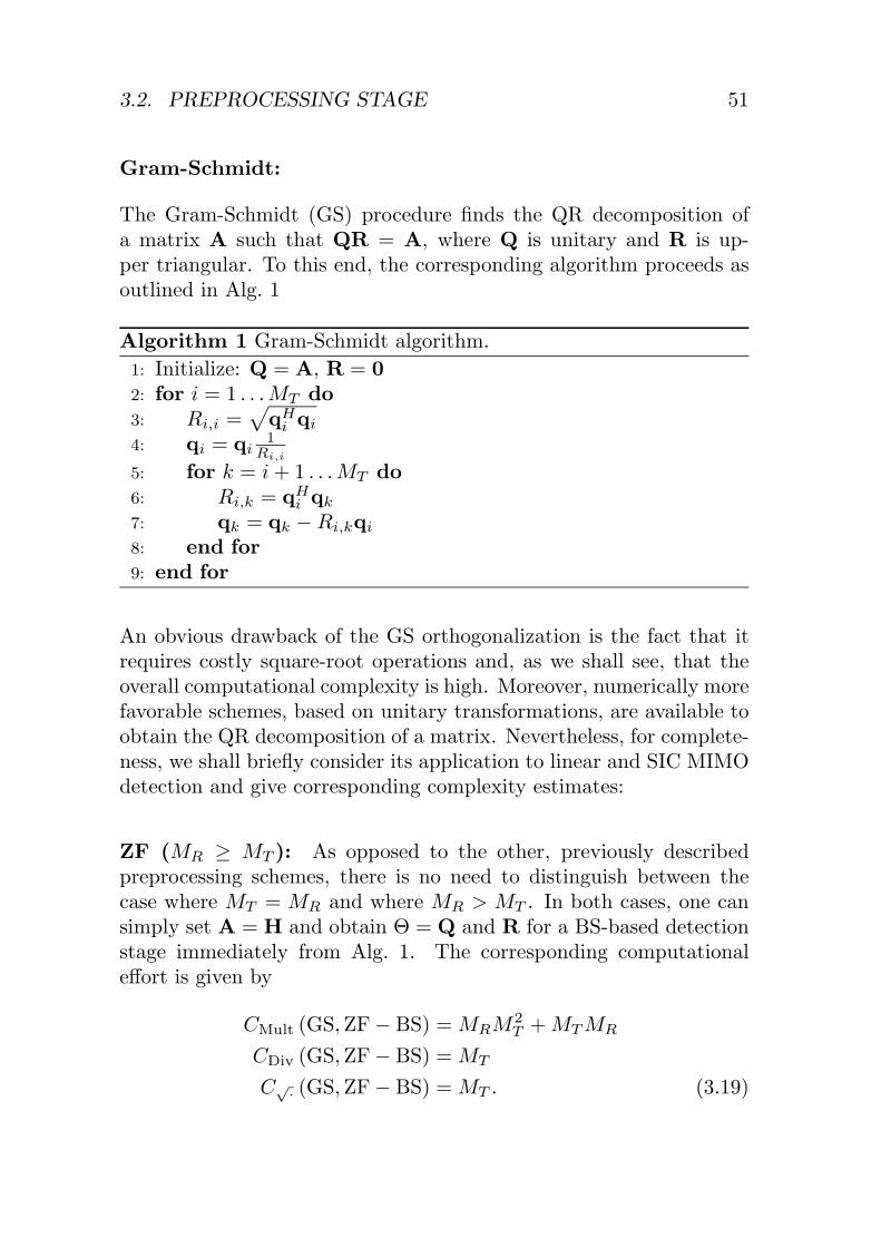
3.2. PREPROCESSING STAGE 51
Gram-Schmidt:
The Gram-Schmidt (GS) procedure finds the QR decomposition ofa matrix A such that QR = A, where Q is unitary and R is up-per triangular. To this end, the corresponding algorithm proceeds asoutlined in Alg. 1
Algorithm 1 Gram-Schmidt algorithm.1: Initialize: Q = A, R = 02: for i = 1 . . .MT do3: Ri,i =
√qH
i qi
4: qi = qi1
Ri,i
5: for k = i+ 1 . . .MT do6: Ri,k = qH
i qk
7: qk = qk −Ri,kqi
8: end for9: end for
An obvious drawback of the GS orthogonalization is the fact that itrequires costly square-root operations and, as we shall see, that theoverall computational complexity is high. Moreover, numerically morefavorable schemes, based on unitary transformations, are available toobtain the QR decomposition of a matrix. Nevertheless, for complete-ness, we shall briefly consider its application to linear and SIC MIMOdetection and give corresponding complexity estimates:
ZF (MR ≥ MT ): As opposed to the other, previously describedpreprocessing schemes, there is no need to distinguish between thecase where MT = MR and where MR > MT . In both cases, one cansimply set A = H and obtain Θ = Q and R for a BS-based detectionstage immediately from Alg. 1. The corresponding computationaleffort is given by
CMult (GS,ZF− BS) =MRM2T +MTMR
CDiv (GS,ZF− BS) =MT
C√· (GS,ZF− BS) =MT . (3.19)

52 CHAPTER 3. LINEAR/SIC DETECTION
For a MM-based detection stage, one must continue to solve RG =QH through BS, which requires an additional effort of MRMT (MT +1)/2 multiplications and MT divisions.
MMSE: Similar to ZF detection for MR ≥MT , one can also avoidthe computation of Ψ for MMSE detection. Instead, one can use anaugmented channel matrix
A =[
H√MTσI
](3.20)
to perform the GS procedure in Alg. 1 in order to obtain Θ as thefirst MR rows of Q and R for a BS-based detection stage. Takingthe sparse nature of the augmented channel matrix into account, thecomputational complexity of the algorithm is given by
CMult (GS,MMSE− BS) =M3
T
3+M2
TMR +M2
T
2+MTMR +
MT
6CDiv (GS,MMSE− BS) =MT
C√· (GS,MMSE− BS) =MT . (3.21)
As for the ZF detection, a MM-based detection stage requires an ad-ditional effort of MRMT (MT +1)/2 multiplications and MT divisionsfor solving RG = QH through BS during preprocessing.
Riccati Recursion
Another approach that can be used to perform preprocessing for MM-based MMSE detection has been mentioned in [39] in a slightly differ-ent context. The algorithm is borrowed from the updating procedureof the Kalman gain in Kalman filtering applications [40]. The basicidea for computing G for MMSE detection is to start from the trivialinverse ofMTσ2I and to obtain (HHH+MTσ2I)−1 through a series ofMT rank-1 updates by using the matrix inversion lemma. To this end,we first initialize the iteration by setting P(0) = 1
MT σ2 I and proceedthen by computing
P(k) = P(k−1)
(I− HH
k HkP(k−1)
1 + �{HkP(k−1)HH
k
})
(3.22)

3.2. PREPROCESSING STAGE 53
for k = 1 . . .MR, where Hk denotes the k-th row of H. Finally, G =P(MR)HH . An interesting property of the above algorithm is that,as opposed to other schemes for direct matrix inversion for MMSEdetection, it requires no explicit upfront computation of the covariancematrix of the received vector Ψ. In the following we shall refer to thisalgorithm as the Riccati recursion algorithm.For evaluating the computational complexity of the algorithm, weshall consider a straightforward implementation of (3.22). The corre-sponding number of multiplications and divisions is given by
CMult(Riccati) =52MRM2
T +52MRMT −M2
T +MT
CDiv(Riccati =MR. (3.23)
We shall later consider the details of the algorithm in Sec. 3.3.1, to-gether with a suitable VLSI architecture and a discussion of the nu-merical requirements.
Complexity Comparison
Fig. 3.5 and Fig. 3.6 show numerical results for the number of multi-plications that are required for the previously described preprocessingalgorithms. The graph in Fig. 3.5 assumes an MMSE receiver with aMM-based detection stage and compares the scaling behavior of thedifferent algorithms as a function of the number of antennas in thesymmetric case of MT = MR. The second chart in Fig. 3.6 focuseson the prominent case of MT = MR = 4 and compares the compu-tational complexity of ZF and MMSE detection with MM and BSarchitectures for the symbol-rate detection stage.
Comparison of Algorithms: As can be seen from Fig. 3.5, allalgorithms under consideration exhibit a very similar computationalcomplexity for MT ≤ 3. Beyond that, the complexity of the Adj/Detmethod starts to show its exponential complexity scaling behaviorwith the number of antennas, which is proportional to 2MT . Amongthe remaining algorithms, the LR-decomposition features the lowestcomputational complexity, followed by the GS procedure (which, how-ever, requires expensive square root operations), and by the Riccati

54 CHAPTER 3. LINEAR/SIC DETECTION
0
100
200
300
400
500
600
700
800
900
1000
2 4 5
Nu
mb
er
of
mu
ltip
lica
tio
ns
M MT R=
63
Adj/Det LR GS Riccati
Figure 3.5: Number of multiplications for MMSE direct matrix inver-sion algorithms with MM-based detection stages for different antennaconfigurations with MT =MR.
recursion. Nevertheless, the ratio of the number of multiplications forlowest- and for the highest complexity scheme is only approximately×1.5, while the nature of the algorithms and thus the required VLSIarchitectures are extremely different. As such architectural differencescan easily make up for a 50% increase in computational complexity,it is fair to say that for a reasonably small number of antennas, noneof the described schemes comes out clearly ahead of all the others.
Complexity Increase from ZF to MMSE: The complexity in-crease from ZF to MMSE detection (and also for the nonsymmetricZF case) is clearly visible in Fig. 3.6. However, while the computa-tional effort for the LR-decomposition increases by a factor of morethan 2.5× when going from ZF to MMSE, the corresponding impacton the complexity of the GS-procedure only corresponds to a factorof 1.3×.
Complexity Increase from BS to MM Based Detection: Allalgorithms under consideration that obtain a set of nulling vectors

3.2. PREPROCESSING STAGE 55
0
20
40
60
80
100
120
140
160
180
200
Nu
mb
er
of
mu
ltip
lica
tio
ns
Adj/Det LR GS Riccati
ZF-BS ZF-MM MMSE-BS MMSE-MM
Figure 3.6: Number of multiplications for direct matrix inversion al-gorithms for ZF and MMSE receivers with BS-based and MM-baseddetection stages in a MIMO system with MT =MR = 4.
for MM-based detection have a complexity that is higher than thoseschemes that only yield a suitable matrix decomposition for a BS-based detection stage. A direct comparison is only possible for the LR-algorithm and for the GS procedure, which essentially carry out the BSprocedure already during preprocessing. The corresponding overheadin terms of the number of multiplications amounts to a complexityincrease of approximately 30-50%.
3.2.2 Unitary-Transformation Based
A major concern with the direct matrix inversion algorithms, de-scribed in Sec. 3.2.1, is the need for a high number precision whichgives rise to a large silicon area in fixed-point VLSI implementations.The two main reasons for these numerical requirements are
� The use of squaring operations and divisions, which lead to asignificant increase of the dynamic range for some intermediatevariables.
� The desire to replace repeated divisions by multiplications with

56 CHAPTER 3. LINEAR/SIC DETECTION
the corresponding inverse in order to reduce the number of costlyoperations. Unfortunately, the latter often entails an enhance-ment of the quantization noise and thus requires a high fixed-point precision.
The use of unitary transformations instead of the conventional meth-ods is well known as a means to alleviate these numerical problems.The reason for this more favorable behavior lies in the fact that, bydefinition, unitary transformations do not alter the length of a vectorand thus cannot lead to an excessive increase in dynamic range orto an enhancement of quantization noise. Algorithms based on suchunitary transformations are available for performing the QR decom-position or singular-value decomposition5 (SVD) [41]. In the contextof MIMO receiver implementation, we are mainly interested in the useof QR decomposition for the channel-rate preprocessing for linear andSIC receivers (including V-BLAST) with a BS-based detection stage6
and for the preprocessing for iterative tree-search algorithms such asSphere Decoding or K-Best decoding.In the following, we shall first introduce the basics of performingQR decomposition with unitary transformations and we establish ap-propriate measures for characterizing their computational complex-ity. Next, it is explained how these unitary transformation algorithmsare applied to efficiently perform preprocessing for MIMO detectionwith minimal computational effort and expressions for the associatedcomplexities are provided. Finally, we shall exploit the fact that theunitary transformation algorithms apply in a very similar way to dif-ferent MIMO detection schemes to obtain a fair comparison of theirimplementation complexities.
QR Decomposition with Unitary Transformations7
The QR decomposition of a MR ×MT dimensional matrix H aimsat finding a unitary matrix Q and an upper triangular matrix R
5E.g., for Eigenmode transmission in MIMO systems with channel state infor-mation at the transmitter.
6Note that MM-based receivers can still be realized by supplementing the QRdecomposition with a unit that performs BS at the channel rate.
7The Gram-Schmidt procedure obtains the QR decomposition with conven-tional arithmetic.

3.2. PREPROCESSING STAGE 57
such that QR = H. To this end, the algorithm recursively appliesa sequence of unitary transformations QH
i to H according to
R(i+1) = QHi R
(i) with R(1) = H. (3.24)
Each transformation is thereby designed to eliminate more subdiago-nal entries until finally R = R(K) = QH
K . . .QH1 H is upper triangular.
The unitary8 matrix QH simply combines all these iterations in asingle step and is readily obtained from
QH = QHK . . .QH
1 I. (3.25)
Unitary Transformations:
Two well known types of unitary transformations are available thatare suitable to zero one or multiple entries of a matrix:
� Householder reflections
� Givens rotations
Householder Reflections: With Householder reflections, the i-thunitary transformation eliminates (i.e., turns to zero) all subdiagonalentries of the i-th column of R(i). This is achieved by choosing QH
i
as
QHi =
(Ii−1 00 Vi
)with Vi = I− 2vivH
i
‖vi‖2(3.26)
and by setting
vi = ri + ‖ri‖e1, (3.27)
whereby ri denotes the (MR−i+1)-dimensional vector that is given bythe diagonal entry and by the subdiagonal entries of the i-th columnof R(i) and where ei is the i-th unit vector. An example that illus-trates how a 4×4 matrix is diagonalized with Householder reflectionsis given in Fig. 3.7. The first Householder reflection is designed toeliminate all but the first entry of the first column of R(1) = R. The

58 CHAPTER 3. LINEAR/SIC DETECTION
QH1 R(1)
QH2 R(2)
QH3 R(3)
H
R
R R R R
0 R R R
0 R R R
0 R R R
R R R R
0 R R R
0 0 R R
0 0 0 R
R R R R
0 R R R
0 0 R R
0 0 R R
R R R R
R R R R
R R R R
R R R R
Figure 3.7: Illustration of the Householder-transformation based QR-decomposition
second transformation leaves the first row unchanged but eliminatesall subdiagonal entries of the second column and so forth.
Unfortunately, the method has two major drawbacks with respect toits implementation: The first problem is the considerable complexityand in particular the requirement for costly divisions and square rootoperations for the computation of (3.26). The second major concernare the stringent numerical requirements for the computation of therequired unitary matrices QH
i which ultimately nullify the favorablenumerical properties of their subsequent application to R(i). To illus-trate these numerical problems, we assume that in practical applica-tions, the term 2/‖vi‖2 in (3.26) must be precomputed once in orderto reduce the number of costly divisions. Unfortunately, postponingthe normalization of vivH
i immediately leads to a large dynamic rangeof the corresponding intermediate results. Moreover, explicitly writ-ing the additive quantization noise on vivH
i as a matrix ∆q and thequantization noise on 2/‖vi‖2 as a scalar δq leads to the following ex-pression, which reveals two potential sources for severe enhancement
8The product of two unitary matrices is again a unitary matrix.

3.2. PREPROCESSING STAGE 59
of quantization noise:
Vi = I− 2vivHi
‖vi‖2+ 2
∆q
‖ri‖2+ 2δqvivH
i . (3.28)
As a result of these considerations, we can conclude that Householdertransformation are difficult to design properly in hardware and cor-responding algorithms are thus not well suited for VLSI implementa-tions.
Givens Rotations: Givens rotations are plain rotations that canbe designed to zero a single element of a matrix at a time. To illustratethe basic idea, consider a two-dimensional real-valued column vectorwhose second entry is to be turned into a zero. The correspondingGivens-rotation (GR) matrix is constructed and applied as follows:(
cosφ sinφ− sinφ cosφ
) (xy
)=
(x′
0
)with φ = atan
y
x. (3.29)
In order to zero a single element r(i)p,n of a matrix R(i) so that after
R(i+1) = Qp,q(φ)R(i) one obtains r(i+1)p,n = 0, GR is performed in the
plane that is spanned by the p-th and another, say the q-th, unit vec-tor, where q �= p. The corresponding GR matrixQp,q(φ) is an identitymatrix in which the entries p, p and q, q are replaced by cosφ and theentries p, q and q, p are replaced by sinφ and − sinφ, respectively:
QHp,q(φ) =
1 0 0
. . ....
...0 . . . cosφ 0 . . . sinφ 0 . . .
0 1 0...
. . ....
0 . . . − sinφ 0 . . . cosφ 0 . . .0 0 1...
.... . .
(3.30)
and the rotation angle φ must be chosen according to
φ = atanr(i)p,n
r(i)q,n
. (3.31)
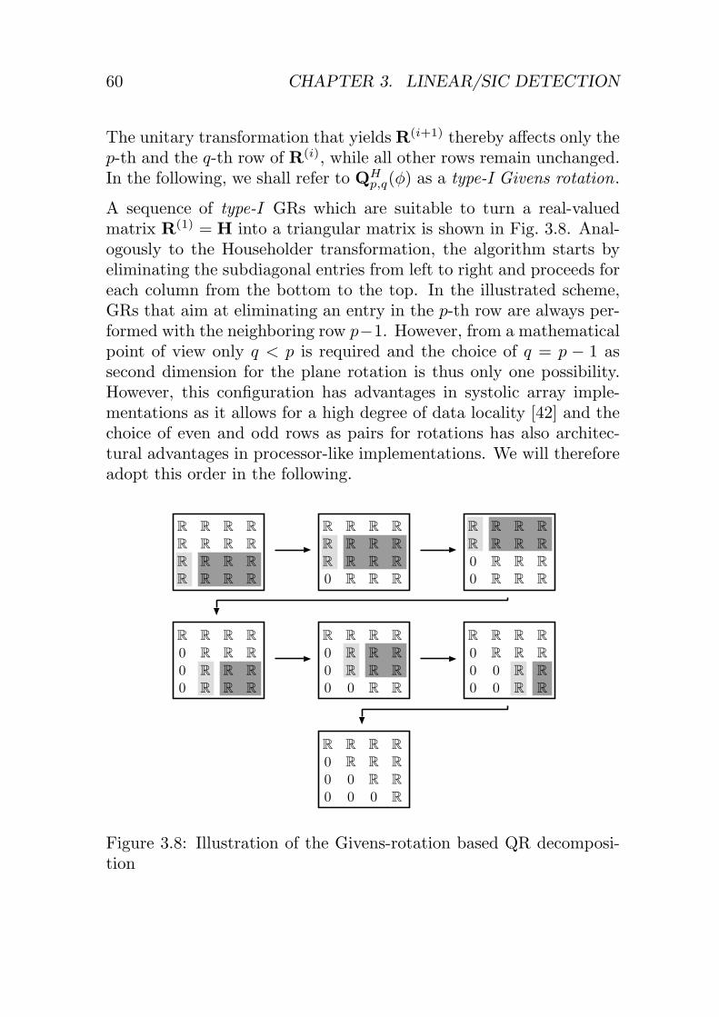
60 CHAPTER 3. LINEAR/SIC DETECTION
The unitary transformation that yieldsR(i+1) thereby affects only thep-th and the q-th row of R(i), while all other rows remain unchanged.In the following, we shall refer to QH
p,q(φ) as a type-I Givens rotation.
A sequence of type-I GRs which are suitable to turn a real-valuedmatrix R(1) = H into a triangular matrix is shown in Fig. 3.8. Anal-ogously to the Householder transformation, the algorithm starts byeliminating the subdiagonal entries from left to right and proceeds foreach column from the bottom to the top. In the illustrated scheme,GRs that aim at eliminating an entry in the p-th row are always per-formed with the neighboring row p−1. However, from a mathematicalpoint of view only q < p is required and the choice of q = p − 1 assecond dimension for the plane rotation is thus only one possibility.However, this configuration has advantages in systolic array imple-mentations as it allows for a high degree of data locality [42] and thechoice of even and odd rows as pairs for rotations has also architec-tural advantages in processor-like implementations. We will thereforeadopt this order in the following.
R R R R
R R R R
R R R R
R R R R
R R R R
R R R R
R R R R
0 R R R
R R R R
R R R R
0 R R R
0 R R R
R R R R
0 R R R
0 R R R
0 0 R R
R R R R
0 R R R
0 R R R
0 R R R
R R R R
0 R R R
0 0 R R
0 0 R R
R R R R
0 R R R
0 0 R R
0 0 0 R
Figure 3.8: Illustration of the Givens-rotation based QR decomposi-tion

3.2. PREPROCESSING STAGE 61
Complex-Valued QR Decomposition with GR
So far we have only considered the QR decomposition of real-valuedmatrices. In the following we shall briefly describe the extension to themore relevant complex-valued case, where each entry of the channelmatrix H lies itself in the complex plane. For the triangularizationof such a matrix with complex-valued entries, the concept of GR isfirst carried over to the complex plane. The corresponding unitarytransformation that zeros the imaginary part of r(i)p,n without affectingany of the other rows of R(i) is given by
QHp (ψ) =
1
. . .
1
e−ψ
1
. . .
1
(3.32)
with
ψ = atan�{r(i)p,n}�{r(i)p,n}
. (3.33)
We shall refer to the corresponding operations as type-II Givens ro-tations. In order to zero a specific entry r
(i)p,n in a complex-valued
matrix, one can now start by applying QHp (ψp,n) and QH
q (ψq,n) toR(i) to first obtain R′(i) according to
R′(i) = QHp (ψp,n)QH
q (ψq,n)R(i). (3.34)
Because the type-II GR has turned the imaginary parts of r′(i)p,n andr′(i)q,n to zero, one can continue as in the real-valued case by apply-
ing (3.30) to obtain R(i+1), with r(i+1)p,i = 0 as desired. As also
r(i+1)q,n ∈ R, one may continue to eliminate r(i+1)
q,n with only a single ad-ditional type-I GR in the complex plane and a regular type-II GR toobtainR(i+2), omittingQH
q (ψq,i+1). An illustration of the first few it-erations for triangularization of a complex-valued matrix according to

62 CHAPTER 3. LINEAR/SIC DETECTION
this scheme is given in Fig. 3.9. The procedure starts with two type-IIGRs, which null the imaginary parts of the two bottom-most elementsof the first column. Next, a type-I GR is applied to the last two rowsto fully annihilate the entry in the bottom-left corner. However, itis noted that the same GR rotation also affects both the real andimaginary parts of the still complex-valued entries in the remainingcolumns. To fully eliminate the next element in the first column, onlyone additional type-II GR is needed, as one of the involved elements isalready real-valued. The algorithm continues according to this schemeuntil all subdiagonal entries are zero and all diagonal entries are realvalued.
C C C C
R C C C
0 C C C
0 C C C
C C C C
R C C C
R C C C
0 C C C
C C C C
C C C C
R C C C
0 C C C
C C C C
C C C C
C C C C
C C C C
C C C C
C C C C
C C C C
R C C C
C C C C
C C C C
R C C C
R C C C
Figure 3.9: Illustration of the Givens-rotation based QR decomposi-tion with complex matrices
Cost of Givens Rotations
In order to analyze the computational complexity of the Givens-rotationbased MIMO detection algorithms, it is necessary to distinguish be-tween the cost that is associated with the computation of the GRmatrix (including the nulling of the corresponding element) and thecost that arises from the application of the GR matrix to another ma-trix. In the following, we will refer to the former as vectoring and onlyto the latter as Givens-rotation operations.
3.2. PREPROCESSING STAGE 63
Vectoring: The vectoring operation can be seen as an atomic oper-ation whose complexity CVec only depends on the implementation butis not data dependent and remains the same for all steps of the algo-rithm. For reasons that will become more clear when the implementa-tion of the vectoring operation is described, CVec already includes thecost for its application to the two-dimensional vector based on whichit is computed.
Rotation: As opposed to the vectoring operation, the GR itself iscomprised of a variable number of vector rotations of two-dimensional,real-valued vectors9 as defined in (3.29). To each of these vector ro-tations we assign a cost of CRot that depends only on the implemen-tation10. The cost of the GR CGR is then given by the number oftwo-dimensional vector rotations, which depends on the type of theGR matrix (cf. (3.30) and (3.32)) and, as we shall see, also on thematrix to which the GR operation is applied.
To illustrate this variable complexity, we first consider a type-I GRmatrix that is defined according to (3.30). Application of QH
p (ψ) to amatrix with MT columns and only nonzero entries in the p-th columnrequires MT two-dimensional vector rotations in the complex plane.Hence, the corresponding complexity is MTCRot. However, QH
p (ψ) isoften applied to a matrix that has only k < MT nonzero entries inits p-th row. Then, the corresponding rotations can often be skippedand the complexity reduces11 to kCRot.
In order to understand the cost of a type-II GR we first assume againthat it is applied to a matrix R(i) with MT columns and complex-valued entries. The operation affects only the p-th and q-th row ofthat matrix and can be split into two parts, by applying the real-valuedQH
p,q(φ) separately to the real- and imaginary parts of R(i). Without
9For type-II GRs, these correspond to the real- and imaginary parts of a com-plex number.
10Note that the entries of the vector to be rotated can be viewed as the real- andimaginary parts of a complex vector, which can be rotated through multiplicationwith a suitably chosen complex complex number. Hence, for some implementationswe expect CRot ≈ CMult.
11It is noted, that depending on the implementation, skipping an unnecessaryoperation may not always lead to complexity reduction, as processing resourcesmay simply be left unused.

64 CHAPTER 3. LINEAR/SIC DETECTION
data dependent optimizations, the corresponding complexity is givenby 2MTCRot. However, if data dependent optimizations can be made,the number of vector rotations can be reduced by one for each columnin which �{r(i)p,n} = �{h(i)q,n} = 0 or �{r(i)p,n} = �{r(i)q,n} = 0. Ifr(i)p,n = h
(i)q,n = 0, two vector rotations can be skipped.
QR-Decomposition for ZF
Algorithm: Using unitary transformations for the preprocessing forZF MIMO detection is straightforward. The algorithm first finds theQR decomposition of the – possibly tall (MR ≥MT ) – channel matrixH, which yields
Q =[Qα Q1
]and R =
[Rα
0
], (3.35)
where H = QR. Next, we are either interested in finding the nullingvectors G for MM-based detection or in directly solving the least-squares detection problem that yields s through BS at the symbolrate. The two corresponding equations are repeated here as follows:
RG = QH and Rs = QHy. (3.36)
Notably, only theMR×MT -dimensional matrixQα is required to solveeither of the two expressions in (3.36). However, with the describedQR decomposition algorithm, Q1 is a side product of the computationof Qα that can, unfortunately, not be eliminated for further complex-ity reduction.
Complexity: In order to determine the complexity of the QR de-composition for ZF detection, we recall that R is computed by recur-sively applying GR matrices to H as in (3.24) and that QH is com-puted by applying the same GRs to the identity matrix I as in (3.25).At this point our complexity measures are CVec(ZF) and CGR(ZF),where the latter is formulated in terms of the number of two-elementvector rotations, each of which has a fixed individual complexity ofCRot.

3.2. PREPROCESSING STAGE 65
The number of vectoring operations follows immediately from thenumber of GRs that are required to transform H into R as partiallyillustrated in the example in Fig. 3.9: Eliminating the subdiagonalentries in the i-th column thereby requiresMR+1− i type-I GRs andMR − i type-II GRs. Hence the total number of vectoring operationsis given by
CVec(ZF) =MT∑i=1
(2 (MR − i) + 1) = 2MRMT −M2T . (3.37)
Computing the cost CGR(ZF) of applying the GR matrices is moreinvolved and requires a careful study of the matrices to which theGRs are applied. These matrices contain a considerable number ofentries which are a priori known to be zero and thus allow to skip asignificant number of vector rotations. For the complexity analysis,it is instructive to consider the operations that are involved in theelimination of the subdiagonal entries in the i-th column of H andin the corresponding update of QH according to (3.25). Fig. 3.10illustrates the structure of the matrices to which the GRs are appliedfor i = 1 . . . 3. For the update ofR, type-I and type-II GRs are appliedto an (MR + 1 − i) × (MT − i) dimensional submatrix with nonzerocomplex entries. The submatrix that is affected in the i-th step bythe update of Q is an upper triangular matrix without the last i− 1rows, whose nonzero entries are complex valued. Only the first update(i = 1) is a special case in which the type-I GRs are only applied tothe sparse identity matrix I. The subsequent type-II GRs then lead tothe transition to the triangular structure. The final cost for all GRsin terms of the number of actually required two-dimensional vectorrotations is given by
CGR(ZF) =32
(MRM2
T +M2RMT
)− 12
(M2
R +MR
)+MR −M3
T −12
(M2
T +MT
). (3.38)

66 CHAPTER 3. LINEAR/SIC DETECTION
R C C C C C C C C C
· R C C C C C C C C
· · C C C C C C C C
· · C C · C C C C C
· · C C · · C C C C
· · C C · · · C C C
× ××
C C C C R · · · · ·C C C C · R · · · ·C C C C · · R · · ·C C C C · · · R · ·C C C C · · · · R ·C C C C · · · · · R
R C C C C C C C C C
· C C C C C C C C C
· C C C · C C C C C
· C C C · · C C C C
· C C C · · · C C C
· C C C · · · · C C
×
a) b)
c)
Figure 3.10: QR decomposition for ZF with MT = 4 and MR = 6.
QR-Decomposition for MMSE
Algorithm: In order to perform QR decomposition with unitarytransformations for MMSE detection we introduce the augmented chan-nel matrix H and the augmented received signal vector y as
H =[
H√MTσIMT
]and y =
[y0
]. (3.39)
The QR decomposition of H yields
H = QR with Q =[Qα Q1
Q2 Q3
]and R =
[R0
](3.40)
Noting that H†y =(HHH+MTσ2I
)−1HHy, the MMSE detector
as given in (2.8) can now be written as the least-squares solution ofy = Hs, which is readily obtained by solving
Rs = QHα y (3.41)

3.2. PREPROCESSING STAGE 67
through BS. Similar to the ZF case, we note that only R and QHα are
actually needed in the detector. Therefore, it is not necessary to applyall GRs to IMT+MR , as in (3.25), which would yield QH . Instead, itis sufficient to apply the GRs to a column-reduced identity matrix
I =[
IMR×MR
0MT ×MR.
](3.42)
As a result of this optimization, only QHα and QH
1 are obtained,whereby the latter is again not required for any further steps, butits computation can also not be avoided. The overall procedure thatyields R and QH
α is illustrated in Fig. 3.11.
C C C C R · · · ·C C C C · R · · ·C C C C · · R · ·C C C C · · · R ·C C C C · · · · R
1 · · · · · · · ·· 1 · · · · · · ·· · 1 · · · · · ·· · · 1 · · · · ·
R C C C C C C C C
· C C C C C C C C
· C C C · C C C C
· C C C · · C C C
· C C C · · · C C
· C C C · · · · C
· 1 · · · · · · ·· · 1 · · · · · ·· · · 1 · · · · ·
R C C C C C C C C
· R C C C C C C C
· · R C C C C C C
· · · C C C C C C
· · · C · C C C C
· · · C · · C C C
· · · C · · · C C
· · · C · · · · C
· · · 1 · · · · ·
R C C C C C C C C
· R C C C C C C C
· · R C C C C C C
· · · R C C C C C
· · · · C C C C C
· · · · · C C C C
· · · · · · C C C
· · · · · · · C C
· · · · · · · · C
QHa
R
Figure 3.11: QR decomposition for MMSE withMT = 4 andMR = 5.
Complexity: As for the QR based ZF detector we obtain an esti-mate of the complexity by counting the number of vectoring operations

68 CHAPTER 3. LINEAR/SIC DETECTION
and the number of two-input vector rotations with nonzero operands,which corresponds to the aggregate cost for the GR operations.With the augmented channel matrix, elimination of the subdiagonalentries of the i-th column of H requires MR vectoring operations fortype-I GRs and another MR vectoring operations for type-II GRs.The total number of vectoring operations for i = 1 . . .MT is thengiven by
CVec(MMSE) =MT∑i=1
2MR = 2MTMR. (3.43)
The resulting GRmatrices are then applied to update R and [Qa Q1]H .
In the i-th iteration, the update of R affects only the entries of an(MR+1)× (MT − i) submatrix, whose last row has only a single real-valued entry, while all other entries in that row are a priori known tobe zero. The update of the unitary matrix affects anMR×MR dimen-sional upper triangular submatrix with complex-valued entries. Thefirst update of [Qa Q1]
H is again a special case, as the correspondingtype-I GRs are applied to the sparse matrix I. The subsequent type-IIGRs then turn the diagonal matrix into a an upper triangular matrixto which the remaining GRs are applied. The total number of vectorrotations is given by
CRot(MMSE) =32
(MRM2
T +M2RMT
)− 12
(M2
R +MR
)(3.44)
The Square-Root Algorithm for V-BLAST
Algorithm: The V-BLAST scheme [18] realizes SIC detection withan ordering that optimizes the BER performance. The original al-gorithm is based on direct matrix inversion and has a high compu-tational complexity that grows as O(M3
TMR). A more efficient andnumerically more stable implementation strategy has been proposedby Hassibi in [21] and has been optimized further for low complexityby Zhu in [43]. Instead of describing the details of the algorithms, weonly note that both methods heavily rely on unitary transformations,which can be implemented using GRs. For further details, the readeris referred to the corresponding references.

3.2. PREPROCESSING STAGE 69
Complexity: With respect to the implementation complexity, wenote that, as opposed to the straightforward QR decomposition algo-rithms, both implementation strategies for the V-BLAST scheme alsorequire multiplication-like operations, such as conventional complex-valued multiplications and norm computations, in addition to the vec-toring and rotation operations for GRs.Our analysis of Hassibi’s algorithm (see [44] for details) shows thatthe exact number of vectoring and rotation operations as well as thenumber of multiplication-like operations is given by
CMult(Hassibi) =M2TMR +
13M3
T +12M2
T +16MT +MTMR
CVec(Hassibi) =2MRMT +M2T − 1
CRot(Hassibi) =MT − 2M2T + 3M
2TMR +
32MTM2
R
+32MRMT +M3
T −MR. (3.45)
An estimate of the computational effort for the reduced-complexityalgorithm by Zhu is given by
CMult(Zhu) =32M2
TMR +13M3
T +12M2
T +16MT
+ 3 +32MRMT + 2MR
CVec(Zhu) =2MRMT +M2T − 1,
CRot(Zhu) =3M2TMR −
12M2
T +12M3
T . (3.46)
Note that, as for the QR decomposition for MMSE and ZF detection,these numbers include only those operations, whose outcome is notknown a priori.
Computational Complexity
As we have seen, the QR decomposition algorithm using unitary trans-formations applies in a very similar way to ZF or MMSE linear detec-tion and SIC (including low-complexity V-BLAST algorithms). Hence,

70 CHAPTER 3. LINEAR/SIC DETECTION
the unitary transformation approach provides an excellent basis for acomparison of the computational effort that is associated with thesedifferent MIMO detection strategies. The chart in Fig. 3.12 pro-vides numerical results for the complexity of the QR preprocessingfor MMSE and ZF MIMO detection as well as for the V-BLAST im-plementations according to Hassibi [21] and Zhu [43]. Our complexitymeasure is the number of vector rotations plus (where needed) thenumber of multiplications (CRot + CMult). The two types of opera-tions exhibit a comparable silicon complexity and, as we shall see inSec. 3.3.2, both can be implemented with complex-valued multiplica-tions. Hence, they can be combined into a single complexity mea-sure. The comparison in Fig. 3.12 neglects the comparatively smallnumber of vectoring operations which, as we shall also see, can behidden in smart implementations behind the much larger number ofmultiplication-like operations.
2 4 6 8
Nu
mb
er
of
op
era
tio
ns
0
1500
3000
3500
2500
2000
1000
500
ZF MMSE V-BLAST (Zhu) V-BLAST (Hassibi)
M MT R=
Figure 3.12: Complexity comparison of unitary-transformation basedMIMO preprocessing algorithms for different antenna configurationswith MT =MR.
Algorithm Comparison: Preprocessing for ZF detection has thelowest computational complexity and the result can be used for linear
3.2. PREPROCESSING STAGE 71
detection and with a BS-based symbol-rate processing. However, thealgorithm also has the lowest BER performance compared to the otherMIMO detection algorithms. A further disadvantage, with respect toits implementation, arises from the fact that the computation of thecorresponding linear estimator G = R−1QH for a MM-based detec-tion stage is numerically difficult, as the diagonal entries of R canbe arbitrarily close to zero, which leads to an unbounded dynamicrange. QR decomposition for MMSE detection involves an almost50% increase in complexity, compared to ZF detection. This resultroughly corresponds to the findings for the complexity increase fromZF to MMSE detection when QR decomposition is implemented us-ing the conventional arithmetic based GS procedure. However, theadvantages of MMSE detection are a better BER performance and– for MM-based detection – the fact that the diagonal entries of Rare lower bounded by
√1/ (σ2MT )/2. At high SNR, one can thus
set σ2 to an implementation-dependent minimum value, which thenserves as a regularization parameter which limits the dynamic rangethat is required for the computation of G. Finally, the algorithms forthe MMSE V-BLAST scheme in [21] and [43] are found to lead toan almost 2.3–2.5× and 1.8–2× increase in computational complexitycompared to the preprocessing for MMSE linear or SIC detection withstraightforward, but suboptimal ordering schemes.
Summary: In summary, one can say that performing preprocessingfor MMSE detection is in general only slightly more complex than forZF. Mainly because of the better numerical properties (limited dy-namic range) and due to the better BER performance it is conculdedthat MMSE detection should always be preferred for MM-based de-tection stages. The square-root algorithm for V-BLAST incurs a con-siderable complexity increase compared to MMSE, and the algorithmhas a significantly less regular structure, which leads to area overheadin VLSI architectures. As SIC schemes with only slightly suboptimalordering (such as sorted-QR) can yield similar BER performance (asillustrated in Fig. 2.7), it is thus concluded that the use of V-BLASTis not very attractive for practical implementations.

72 CHAPTER 3. LINEAR/SIC DETECTION
3.2.3 Iterative Methods
Iterative methods for solving linear systems of equations are an alter-native approach to direct or unitary-transformation based methodsfor computing the linear estimator G for MM-based MIMO detec-tion. Other than direct methods, such algorithms do not yield thefinal, exact result in a finite number of steps. Instead, iterative ma-trix inversion algorithms proceed recursively to (hopefully) convergecloser and closer toward the solution. The complexity of such algo-rithms is given by the complexity of a single iteration and by thenumber of iterations that are needed to converge to a result with re-quired accuracy. In the following, we shall consider the use of iterativeschemes for solving (3.9), which corresponds to both MMSE and toZF detection with MR ≥MT .
Jacobi and Gauss-Seidel
Algorithm: The Jacobi and the Gauss-Seidel methods are based onthe same fundamental idea. Both algorithms start by decomposing thematrix Ψ into a matrix A and a matrix B, such that A + B = Ψ.Each iteration of the algorithm then solves
AX(i) = HH −BX(i−1) (3.47)
for X(i). If the algorithm converges, G = X(∞) = (Ψ)−1HH .In the Jacobi method A is chosen as a diagonal matrix that containsonly the diagonal elements of G and B = G − A. As A−1 can beprecomputed once, a single iteration requires CMult(Jacobi) =M2
TMR
multiplications. The advantage of the scheme with respect to its im-plementation is that it supports a very high degree of parallelism.However, unfortunately, convergence is extremely slow.The Gauss-Seidel method converges significantly faster compared tothe Jacobi method. The improvement is achieved by choosing A asthe lower triangular part of Ψ so that B = Ψ − A is strictly up-per triangular. Each iteration now involves back substitution, whichrequires the same number of multiplications as the Jacobi scheme:CMult(Gauss-Seidel) =M2
TMR. Unfortunately, BS is less suited foran implementation as data dependencies now limit amount of paral-lelism that can be explored.

3.2. PREPROCESSING STAGE 73
Complexity and Convergence: The iterative algorithm in (3.47)entails a tradeoff between the computational complexity of the channel-rate preprocessing (which is governed by the number of iterations) andthe BER performance of the system, which is ultimately limited bythe residual error on the linear estimator G and shows up as an errorfloor. In order to quantify this tradeoff, let us study the behavior ofthe overall MIMO system when a finite number of iterations K is em-ployed. For the analysis, the linear MMSE estimator is first modeledas
G = G+Gq, (3.48)
where G is the error-free solution and the matrix Gq describes theresidual error after K iterations. To analyze the error floor, the high-SNR case (σ2 → 0) is considered. The signal after linear detectionwith the distorted estimator can then be written as the sum of thetransmitted vector symbol s and an additive noise vector e
x = s+ e (3.49)e = Zx with Z = GqH (3.50)
Slicing is performed independently on each entry of x and a symbolerror occurs, when either the real or imaginary component of the errorei exceeds half of the minimum distance between two constellationpoints as shown in Fig. 3.13. Under the assumption of ei being circularsymmetric, the symbol-error probability can be computed as
Ps = 1− P(|� {ei}| <
dmin
2
)2
. (3.51)
Unfortunately, the distribution of the random variable |� {ei}| isnot known so that an exact expression for (3.51) cannot be derivedanalytically. Therefore, only an approximation through an outagecriterion is attempted. To this end, it is first noted that for a givenGq and the corresponding Z the variance of |� {ei}| is given by σ2e/2as
σ2e2=
MR∑j=1
12|Zi,j |2 , (3.52)

74 CHAPTER 3. LINEAR/SIC DETECTION
dmin
dmin
2
eidmin =
2√2
1√MT
QPSK2√10
1√MT
16 − QAM2√42
1√MT
64 − QAM
Figure 3.13: Constellation points and x before slicing (left) and dmin
in a system with MT transmit antennas (right).
assuming the entries of x are zero mean with variance one12. Theapplication of the Chebyshev bound to (3.51) indicates that one canassume that communication fails, whenever σe/
√2 > dmin/2, because
Pe approaches one. The corresponding probability for this event as afunction of the number of iterations K can be obtained through sim-ulations. The graph in Fig. 3.14 shows the corresponding, empiricallyobtained, inverse cumulative distribution function (ICDF) of σe/
√2
from which the probability of an outage event for a certain K can eas-ily be identified. Clearly, a very large number of iterations is neededto reduce the error on the estimator to a degree that allows for reli-able communication. As only a single iteration is nearly as complexas most direct methods, it can be concluded that Gauss-Seidel is notefficient for applications in MIMO communications.
Schultz-Hotelling Method
Algorithm: The Schultz-Hotelling method is essentially a Newton-Raphson approach to matrix inversion. The algorithm starts with aninitialization X0 and proceeds as follows:
X(i) = 2X(i−1) −X(i−1)RyyX(i−1) (3.53)
12Based on the assumption that the entries of H are i.i.d., proper complexGaussian distributed with variance one and that the total transmitted power hasbeen normalized to one.

3.2. PREPROCESSING STAGE 75
P( σ
e√
2>
x)
K=
1
K=
5K
=10
0 0.1 0.2 0.3 0.4 0.5 0.610
-2
10-1
100
x
dm
in/2(6
4−
QA
M)
dm
in/2(1
6−
QA
M)
Figure 3.14: ICDF of σe/√2 with the Gauss-Seidel method for
MT =MR = 4 with the number of iterations as parameter. For ref-erence, half of the minimum distance for 16-QAM and 64-QAM arealso shown.
Complexity and Convergence: Per iteration M2T (MT + 1) mul-
tiplications are needed. After a sufficient number of iterations K,the final result is computed as G = X(k)HH , requiring an additionalM2
TMR multiplications. The choice of the initialization is therebycritical to ensure convergence, optimum choices are in general costlyto implement in practice. In the following X0 = 0.1I has been chosenfrom experiments for a 4×4 scenario. Following the same analysis asfor the Gauss-Seidel algorithm, the tradeoff between computationalcomplexity and BER is illustrated in Fig. 3.15. The sharp drop of theICDF of the error after a given number of iterations indicates that thealgorithm is more robust against channel realizations that would lead

76 CHAPTER 3. LINEAR/SIC DETECTION
0 0.1 0.2 0.3 0.4 0.510
-3
10-2
10-1
100
x
K=
1
K=
5
K=
10
P( σ
e√
2>
x)
dm
in/2(6
4−
QA
M)
dm
in/2(1
6−
QA
M)
Figure 3.15: ICDF of σe/√2 with the Schultz method for
MT =MR = 4 with the number of iterations as parameter. For ref-erence, half of the minimum distance for 16-QAM and 64-QAM arealso given.
to slow convergence with the Gauss-Seidel scheme. In other words,there are fewer situations, where the algorithm stays far away froma good solution if a large number of iterations is applied. Despitethis favorable property, a large number of operations is still requiredto achieve good BER performance so that the overall computationalcomplexity is too high to compete with other direct schemes.
3.2.4 Adaptive Methods
Finally, adaptive methods use an iterative procedure to adjust Gin such a way that the residual error between the signal after lin-

3.2. PREPROCESSING STAGE 77
ear MIMO detection and a reference sequence is minimized accordingto some suitable error criterion. No explicit estimation of the chan-nel is therefore needed as illustrated in the high-level block diagramin Fig. 3.16 which compares channel estimate based techniques withadaptive techniques. For the implementation of the adaptation loop, avariety of well established algorithms from adaptive equalization andfrom acoustic echo cancellation can be adopted. The most well knownschemes are based on LMS or RLS, or thereof derived methods withreduced complexity or improved convergence properties.
MIMODetection
Compute thelinear estimator
Channelestimation
Estimatoradaptation
MIMODetection
y y
H
GG
Referencesequence
Referencesequence
x x
Figure 3.16: Block diagram of a conventional nonadaptive (left) andan adaptive (right) linear MIMO detector.
From a VLSI perspective, adaptive techniques often have the advan-tage of relaxed numerical requirements compared to channel estima-tion and direct matrix-inversion based techniques. The main reasonfor this is the fact that typically the output of the adaptation loophas a low-pass characteristic with a bandwidth that is only a frac-tion of its input rate, as the channel changes only slowly compared tothe symbol rate. On the algorithmic level, the bandwidth of the loopdetermines the residual error on the estimate. In an actual implemen-tation, the low-pass characteristic also removes a significant portionof the quantization noise from the adaptation datapath which relaxesthe numerical requirements and reduces the silicon complexity. At thesame time, the high input rate is the drawback of adaptive algorithms.Operations need to be performed on a high rate, which may requiresignificant parallel processing and can lead to high power consumptiondue to high clock rates.The main problem of adaptive schemes in wireless communications isthe initial adaptation phase, where no prior knowledge of G is avail-

78 CHAPTER 3. LINEAR/SIC DETECTION
able as a starting point so that time is needed to converge. However,in particular in packet-based TDMA systems the channel between aparticular transmitter and a receiver may change significantly betweentwo subsequent packets. As also no training data is available duringthat interval to track these changes, the algorithm has to convergeanew, every time a new packet is received. As a consequence, signifi-cant latency may be introduced at the beginning of each packet. Onthe other hand, adaptive algorithms are attractive for systems wherecontinuous (superimposed) training is available, so that changes inthe channel can be tracked. An example are MIMO-CDMA systems[45, 46]. There, training is broadcast continuously on the downlink,while on the uplink training is also available at all times from all users,separated by their respective codes. A VLSI implementation of sucha system, using adaptive methods to adjust coefficients of a linearMIMO equalizer, has been presented in [47]. However, in this workthese algorithms are not further pursued.
3.3. VLSI IMPLEMENTATIONS 79
3.3 VLSI Implementations
In order to assess the true silicon complexity of linear detection schemes,we shall consider actual VLSI implementations and the correspondinghardware architectures in the following.
3.3.1 Implementation of the Riccati Recursion
Our first reference design is intended to perform linear MMSE detec-tion in systems in which preprocessing latency is critical, but wheredetection and preprocessing are never carried out in parallel. In suchsystems (e.g., in packet based MIMO-OFDM systems [48]), the com-putation of the linear estimatorG must be optimized for speed. How-ever, the hardware for the preprocessing may also be reused for thesubsequent symbol-rate detection. A second application for direct ma-trix inversion based methods are systems, where linear MIMO equal-ization and detection must be separated, so that the use of the nu-merically more stable QR decomposition in conjunction with BS-baseddetection is not an option. Examples for such systems are multicarrierCDMA systems or conventional CDMA systems with low-complexitylinear frequency domain equalization [49].
Preprocessing Algorithm
The proposed architecture to compute the MMSE estimator G isbased on the Riccati recursion. In order to map the algorithm tohardware, its compact mathematical description in (3.22) is first de-composed into a series of operations as shown in Alg. 2. This sequenceis designed to minimize the number of costly divisions, while at thesame time keeping the number of multiplications low and minimiz-ing the dynamic range of intermediate results. Note that also to thisend, the division in (3.22) is implemented using pseudo floating-pointarithmetic, as described in step 5) of Alg. 2.

80 CHAPTER 3. LINEAR/SIC DETECTION
Algorithm 2 Riccati recursion algorithm1: P(0) = 1
MT σ2 I2: for k = 1 . . .MR do3: g = P(k−1)HH
k
4: S = 1 + �{Hkg}5: Se = �log2 S�, Sm = 2Se/S6: g = Smg7: P(k) = P(k−1) − ggH2−Se
8: end for9: G = P(MR)HH
Architectural Choices
The choice of a suitable hardware architecture for the implementationof Alg. 2 depends on the system requirements and on the availablearea.
Decomposed Architecture: The most area-efficient solution is afully decomposed, processor-like architecture. However, such a trivialminimum-area solution can often neither meet the low-latency require-ments for the preprocessing nor the throughput requirements for thesymbol-rate detection.
Fully Parallel Architecture: A highly parallel architecture achieveslower latencies and higher throughput. As data dependencies do notallow for parallel processing across the individual steps in Alg. 2, thehighest degree of parallel processing is achieved by allocating suffi-cient resources to process the most complex step in a single cycle.Such an approach has several drawbacks: First, the required siliconarea is extremely high. Second, memories need to be implementedbased on register files, to provide sufficient access bandwidth. Finally,it is noted that some steps in the algorithm require a much larger num-ber of operations compared to other steps. Hence, as resource sharingacross the individual steps is difficult, a considerable percentage ofthe processing resources will be idle most of the time and hardwareutilization will thus be poor.

3.3. VLSI IMPLEMENTATIONS 81
Moderately Parallel Architecture: A compromise between thedecomposed and the fully parallel architecture is found with a moder-ately parallel architecture in which the number of processing resourcesis chosen in such a way that their average utilization is high in almostall steps of the algorithm. Most of the steps in the Riccati recursionbased matrix inversion require either MT or a multiple of MT multi-plications. Hence, choosing an MT -fold degree of parallelism will leadto a decent hardware utilization.
Implementation of a Moderately Parallel VLSI Architecture
In the following, we shall briefly describe the mapping of the prepro-cessing and the detection onto a moderately parallel VLSI architectureand analyze the number of cycles that are required for the operations.
Architecture: The high-level block diagram of the proposed mod-erately parallel architecture is shown in Fig. 3.17(a). The circuit em-ploys MT identical processing elements (PEs) arranged in a circu-lar array and a common 1/
∑-block that computes the additions in
step 4) and the pseudo floating-point division in step 5). The connec-tions in the array are local, meaning that only neighboring PEs areconnected with each other. However, as combinatorial paths do existbetween the inputs and the outputs of the individual PEs and due tothe connections to the common 1/
∑-block the structure can not be
classified as a systolic array.Each PE mainly contains a complex-valued multiplier, an adder andsome local storage registers as shown in Fig. 3.17(b). All intermediatevariables (g, g, and P) are stored in an equally distributed way amongthe PEs. The arrangement of the entries of the matrix P therebyfollow the assignment illustrated in Fig. 3.18 to ensure data localityduring operation and to exploit the Hermitian structure of the matrixto reduce storage requirements.
Preprocessing: The computation of the MMSE estimator startswith the loop between step 2) and step 8) in Alg. 2. During the k-th iteration the entries of the k-th row of H must be presented tothe inputs of the corresponding PEs as shown in Fig. 3.17(a). A

82 CHAPTER 3. LINEAR/SIC DETECTION
a)b)
Mem
0
+/->>
0
Sm
ρ=
1M
Tσ2
−S
e
gi
P
gi
ρ
ρ
Hk
,iG
i,k
/s
i
Opt
iona
l pi
pelin
e re
gist
er
yk
Hk
,1
Hk
,2
Hk
,i
Hk
,MT
G1
,k
G2
,k
Gi,k
GM
T,k
yk
1 ∑
PE
(MT)
PE
(1)
PE
(i)
PE
(2)
Sm
,−
Se
Upper ring
Lower ring
Upp
er r
ing
Low
er r
ing
to1/
∑
Figure 3.17: Block diagram of a moderately parallel architecture forthe Riccati recursion based matrix inversion and for linear detection.

3.3. VLSI IMPLEMENTATIONS 83
P1,1 P1,2 P1,3 P1,4
P2,1 P2,2 P2,3 P2,4
P3,1 P3,2 P3,3 P3,4
P4,1 P4,2 P4,3 P4,4
PE1PE2
PE3PE4
PE1
PE2
PE3
P1,1 P1,2 P1,3 P1,4 P1,5
P2,1 P2,2 P2,3 P2,4 P2,5
P3,1 P3,2 P3,3 P3,4 P3,5
P4,1 P4,2 P4,3 P4,4 P4,5
P5,1 P5,2 P5,3 P5,4 P5,5
PE1PE2
PE3PE4
PE1
PE2
PE3
PE5
PE4
MT = 4MT = 5
Figure 3.18: Distribution of the entries ofP across the PEs forMT = 4and MT = 5.
separate memory bank is thereby associated with each of the PEs. Theprocedure for the computation of the matrix-vector multiplication instep 3) is illustrated in Fig. 3.19. In the first cycle, the first PE usesthe upper ring to broadcast Hk,1 to all other PEs. These multiplyHk,1 with their respective entry of the first column of P(k−1) andstore the result in the g register of the neighboring PE. In the secondcycle, the second PE broadcastsHk,2 to the other PEs, which multiplyit with their respective entries of the second column of P(k−1), addthe content of their g register, and store the result again in the gregister of the neighboring PE. This procedure continues for a totalof MT cycles. Only in the first iteration (k = 1) a single cycle issufficient to compute g due to the initialization of P(0) with a diagonalmatrix in step 1). The multiplications in step 4) can be carried out in
P1,1HHk,1 +P4,2H
Hk,2 +P3,3H
Hk,3 +P2,4H
Hk,4 = [PHH
k ]1P2,1H
Hk,1 +P1,2H
Hk,2 +P4,3H
Hk,3 +P3,4H
Hk,4 = [PHH
k ]2P3,1H
Hk,1 +P2,2H
Hk,2 +P1,3H
Hk,3 +P4,4H
Hk,4 = [PHH
k ]3P4,1H
Hk,1 +P3,2H
Hk,2 +P2,3H
Hk,3 +P1,4H
Hk,4 = [PHH
k ]4
Cycles
PE(1)
PE(2)
PE(3)
PE(4)
Figure 3.19: Procedure to compute step 3) in Alg. 2 for MT = 4.

84 CHAPTER 3. LINEAR/SIC DETECTION
parallel in a single cycle on the individual PEs. The summation of theresults that yields S is absorbed into the 1/
∑block, which performs
the addition together with the execution of the pseudo floating-pointdivision in step 5) within CDiv cycles. The computation of g fromg in step 6), using the result from step 5) can again be performedin a single cycle on the individual PEs. step 7) is carried out usingMT cycles in each of which one entry of g is broadcasted to all PEsthrouhg the upper ring, while the entries of g circulate through thelower ring. While theoretically, only MT (MT + 1)/2 cycles would berequired, the architecture uses M2
T cycles for the computation. Thematrix multiplication of P(MR) with HH in step 9) is computed in asseries of MR matrix-vector multiplications each of which is identicalto step 3). The entries ofH are again applied to the inputs of the PEsrow-by-row so thatG is output column-wise, as shown in Fig. 3.17(a).With this scheme it is possible to replace the kth row ofH with the kthcolumn of G, so that no extra memory is required to store the MMSEestimators. This memory optimization is particularly important whenthe number of channel matrices is high as this is typically the case forexample in MIMO-OFDM systems. The overall number of cycles thatis required to compute Alg. 2 with the presented architecture is givenby
tcpd =MR(3MT + 2)−MT + 1 +MRCDiv. (3.54)
Detection: A significant advantage of the conventional arithmeticbased architecture is the fact that, once preprocessing is complete, thesame hardware can be reused efficiently to perform the matrix-vectormultiplication x = Gy for the symbol-rate detection. To this end,the matrix G is read back from the memory, one column at a time.The entries of the k-th column of G are presented to the PEs togetherwith the k-th entry of the received vector y which is broadcast to allPEs. The result x is then available after MR cycles.
Pipelining: Despite the recursive nature of the Riccati recursionalgorithm, pipelining can be introduced to reduce the critical path inorder to allow for higher clock rates. To this end, an additional regis-ter is added to the original architecture as shown in Fig. 3.17(b). The
3.3. VLSI IMPLEMENTATIONS 85
potential increase in clock speed depends on the quality of the place-ment of the pipeline register in the logic. Unfortunately, pipeliningof the recursive matrix inversion algorithm also requires the insertionof additional cycles to flush the pipeline after the operations that areassociated with steps 3), 4), 6), 7) and 9) of Alg. 2. As a result, thenumber of clock cycles for the preprocessing in (3.54) increases to
tcpd(Riccati) =MR(3MT + 6)−MT + 2 +MRCDiv (3.55)
and the number of clock cycles for the division CDiv also needs to beincreased according to the shorter cycle time.
Fixed-Point Considerations
A critical aspect in the VLSI implementation of matrix inversion al-gorithms with fixed-point arithmetic are the numerical issues whichto a large extent determine the final silicon complexity of the corre-sponding circuits. The intermediate variables in Alg. 2 show signif-icant differences in their dynamic range requirements. Hence, it ismandatory to perform the partitioning between integer and fractionalbits for each of them individually to efficiently utilize the accuracy ofthe arithmetic units in the PEs. The number of integer bits for eachvariable can be determined analytically to ensure that no overflowsoccur. Once the number of integer bits is known for each variable, thecorresponding number of fractional bits is given by the width of thedatapath so that only a single fixed-point design parameter remains tobe optimized by means of Monte-Carlo simulations. This parameterthen determines the complexity/performance tradeoff for a particularimplementation.
Dynamic Range of G: Before considering the dynamic range re-quirements of the different variables in detail, let us start with thedynamic range of the MMSE estimator itself as given in (2.8). It canbe shown that the real and imaginary parts of the entries of G arealways upper bounded by
max |��{Gi,j}| <12
√1
σ2MT, (3.56)
86 CHAPTER 3. LINEAR/SIC DETECTION
where �� denotes either the real or the imaginary part of a complex-valued number. Unfortunately, the noise variance σ can in principlebecome arbitrarily close to zero so that our bound goes to infinity.However, σ2 → 0 corresponds to SNR → ∞, which is never the casein real systems. Hence, we can safely assume a maximum operatingrange in terms of SNR which yields a corresponding σ2min = 1/SNRmax.For all cases where σ2 < σ2min we then simply set σ2 = σ2min, whereσ2min now basically serves as a regularization parameter that guaran-tees a minimum condition number for the matrix to be inverted.
Input Normalization: In order to determine the number of integerbits for all intermediate variables, the dynamic range of the inputsalso needs to be defined. As our system model assumes that thereal and imaginary parts of the entries of the channel matrix H areGaussian distributed it is clear that these variables have an infinitedynamic range. Two common approaches are available to deal withthis problem:
1. A sufficiently large number of integer bits can be used to en-sure that overflows occur only rarely and do therefore not affectsystem performance.
2. Automatic gain control adjusts the data to the available num-ber of integer bits with an appropriate scaling factor, similar tofloating-point implementations. However, the complexity asso-ciated with true floating-point arithmetic can often be avoidedwith block floating-point [50] implementations. This compromisebetween accuracy and circuit complexity chooses a common scal-ing factor (exponent) for an entire set of variables (e.g., for allentries of a matrix).
Practical systems use almost always a combination of both techniques,depending on the cost of additional bits. Spare bits are used wherethe cost per bit is low. AGC is applied where extra bits are expen-sive in terms of additional hardware (e.g., in a receiver before theA/D converters and before the main signal processing chain). Forthe subsequent analysis of the fixed-point requirements of the Ric-cati recursion algorithm, a block floating-point representation of the

3.3. VLSI IMPLEMENTATIONS 87
channel matrix is assumed. In the system under consideration, thecorresponding common gain parameter α is determined for all entriesof the matrix H according to
α = 1/max (max |� {Hi,j}| ,max |� {Hi,j}|) . (3.57)
Preprocessing for MMSE detection is now performed on the scaledchannel matrix H = αH whose entries are guaranteed to have realand imaginary parts smaller than one, so that no integer bits arerequired. However, scaling H by α also requires scaling σ2 by α2 sothat one obtains G = (1/α)G at the output of the preprocessing unit.The corresponding block diagram is shown in Fig. 3.20.
α
α2
σ2
MMSE
AGC
α
GH GH
Figure 3.20: Normalization architecture for MMSE detector.
As the input normalization of the matrix H also affects the noisevariance σ2, the dynamic range computation for the output of thepreprocessing unit needs to be revisited. When the scaling is takeninto account, the entries of G are bounded by
max |��{gi,j}| <12
√1
σ2MTwith σ2 = α2σ2 (3.58)
While the lower bound σ2min on the noise variance parameter ensuresthat σ2 cannot go all the way to zero, the scaling parameter α cannow cause the dynamic range to go to infinity. In order to avoidthis problem, one could insist that α > αmin in the AGC and resortto saturating those entries of H which cannot be scaled sufficiently.However, the corresponding nonlinear distortion is highly undesirable

88 CHAPTER 3. LINEAR/SIC DETECTION
and allowing α to be small, but to enforcing a minimum σ2min on σ2
instead turns out to be a better solution which leads to a more gracefuldegradation of the BER performance. In the following, this σ2min isreferred to as the regularization parameter of our implementation.
Integer Bits: Assuming the above input normalization, the numberof integer bits that are required to represent the entries of the inter-mediate variables and the final result G without overflows are given inTbl. 3.2. The corresponding analysis thereby relies on the knowledgethat the matrices P(k) are semidefinite and uses the fact that theirlargest eigenvalue is always bounded by λmax(P(k)) < 1/(MT σmin).
Table 3.2: Required integer bits for intermediate variables in the Ric-cati recursion algorithm.
Variable Integer bits Variable Integer bits
G log2(12
√1
σ2minMT
)P log2
(1
σ2minMT
)g, g log2
(√2
MT
1σ2min
)S log2
(2
σ2min
)
Choosing the Design Parameters: Due to the necessary normal-ization procedure, the optimization problem of finding a good tradeoffbetween fixed-point performance and hardware complexity now actu-ally depends on two design parameters:
1. The regularization parameter σ2min and
2. the width of the datapath which is given by the width WW ofthe real-valued multipliers that constitute the complex-valuedmultipliers in the PEs.
The regularization parameter σ2min is chosen first. Assuming a floating-point implementation of the algorithm, this lower bound on the scalednoise variance induces an error floor that corresponds roughly to theBER performance that is achieved at an SNR of 1/σ2min. Hence, the

3.3. VLSI IMPLEMENTATIONS 89
Table 3.3: VLSI implementation results for the Riccati recursion al-gorithm for MMSE detection in a 4×4 MIMO system.
Not pipelined: CDiv = 4, tcpd = 69
σ2min WW Area [GE] Clock freq. Time/inv. AT-product
1/511 18 69K 101 MHz 0.68µm 0.047
1/1023 19 75K 96 MHz 0.72µm 0.054
1/2047 20 79K 94 MHz 0.73µm 0.058
1/4095 21 85K 93 MHz 0.74µm 0.063
Pipelined: CDiv = 4, tcpd = 69
σ2min WW Area [GE] Clock freq. Time/inv. AT-product
1/511 18 73K 176 MHz 0.58µm 0.042
1/1023 19 78K 170 MHz 0.60µs 0.047
1/2047 20 82K 170 MHz 0.60µs 0.049
1/4095 21 89K 167 MHz 0.61µs 0.054
parameter defines the SNR operating range of the MMSE detector. Inthe second step, Monte-Carlo simulations are used to determine theminimum required width of the datapath WW in such a way that theadditional BER performance loss from fixed-point quantization errorsis negligible.
Implementation Tradeoffs: The tradeoffs between the BER per-formance and implementation complexity are illustrated for a 4×4MIMO system. Fig. 3.21 gives simulation results for 16-QAM modu-lation when the design parameters σ2min and WW are chosen accord-ing to the above presented methodology. The corresponding siliconarea and the times that are required for the computation an MMSEestimator are given in Tbl. 3.3 for a 0.25µm technology.
With respect to the fixed-point requirements it can be observed fromFig. 3.21 and from the table therein that a considerable accuracyis required in order to achieve a reasonable SNR operating range(WW ≥ 18 bit for 27 dB SNR). However, every increase of this rangeby 3 dB then only requires one additional bit in the datapath. Thecorresponding impact on the clock frequency and thus on the compu-

90 CHAPTER 3. LINEAR/SIC DETECTION
Figure 3.21: MMSE performance in a 4×4 system with 16-QAMmodulation for different SNR operating ranges and datapath widths(10’000 channel realizations).
tation time is small because the delay of a multiplier is a logarithmicfunction of the width of its operands. Nevertheless, the gatecount ofthe multipliers, which dominate the area of the design, grows quadrat-ically with the number of bits so that reaching a high accuracy quicklyleads to considerable silicon area (cf. Tbl. 3.3).
The main architectural choice is between using a pipelined or a un-pipelined PE architecture. From Tbl. 3.3 it can be observed thatpipelining (with manual retiming) allows to increase the clock rate bya factor of almost 1.7 from 93–101 MHz to 167–176 MHz. Automaticretiming is likely to reach almost a factor of two. However, it is alsoobserved that for the computation of the MMSE estimator the gain

3.3. VLSI IMPLEMENTATIONS 91
from the shorter critical path (in terms of computation time and interms of the AT-product) remains small due to the larger numberof cycles. A more significant performance improvement is achievedwhen the circuit operates in the detection mode, computing x = Gyat the symbol rate. In this case, no pipeline bubbles need to be in-serted so that one can take full advantage of the higher clock rate toincrease throughput. For example, the unpipelined reference designsin Tbl. 3.3 can process 23–25 million vectors per second, while thepipelined designs achieve 42–44 million vectors per second.
FPGA Implementation:
For the implementation of the design (for MT = MR = 4) on aXILINX XC2V6000-6 FPGA, WW = 18 was chosen as the pro-grammable device contains hardwired multipliers of that size. Thepipelined version operates at a clock speed of 40 MHz and thus re-quires 2.2µs for the computation of one MMSE estimator. In detec-tion mode, it reaches a throughput of 10 million received vectors persecond. In terms of area, the circuit consumes 16 out of 144 multipliersand 3’416 logic slices out of a total of 33’792.The described circuit is employed in the ETH real-time MIMO-OFDMtestbed [48] which is a 4×4 MIMO-OFDM system with 64 tones (52of which carry data) in a 20 MHz bandwidth. The setup is basedon the IEEE 802.11a SISO standard and the framestructure is anextension thereof to support training for multiple antennas. The real-time capable receiver, fully implemented in an FPGA, employs twoMMSE units to perform the channel rate preprocessing in 57µs (i.e.,14 OFDM symbols) and the MIMO detection at a rate of 20 Mvps.

92 CHAPTER 3. LINEAR/SIC DETECTION
3.3.2 Implementation of QR Algorithms
In Sec. 3.2.2 it has been argued that QR decomposition can be em-ployed to perform linear detection and SIC in MIMO systems withpotentially fewer numerical problems compared to direct matrix in-version algorithms. Moreover, QR decomposition is also required inthe preprocessing stage of the iterative tree-search algorithms whichcan attain full ML performance. Hence, the low-complexity imple-mentation of the algorithm is a matter of particular interest.We start our discussion with the description of a class of applicationsthat has already led to numerous implementations and publications ofarchitectures for QR decomposition and we highlight the differences tothe MIMO detection problem at hand. Next, the architectural choicesthat are available for the implementation of QR decomposition algo-rithms are briefly summarized and the most suitable approach, giventhe boundary conditions of a typical MIMO system, is highlighted.Subsequently, the register transfer level (RTL) architecture and thecircuit-level implementation of the required vectoring and vector ro-tation operations are considered and the associated design space isexplored. Finally two reference implementations are described in de-tail, which were designed for plain QR decomposition and for QRdecomposition for MMSE detection, giving preference to area and de-lay, respectively.
Related Work
In the past, the QR algorithm has received significant attention in thecontext of adaptive RLS filtering, multiantenna adaptive beamforming[51] and for radar applications [52]. All of these systems require thesolution of a linear least-squares (LS) problem of the form
u = Aw, (3.59)
where the number of rows in the tallM×N matrixA (M � N) and inthe observed vector u grow rapidly at the sampling rate. The weightvector w is to be found in such a way that the mean squared erroris minimized, once M reaches a certain target. The problem can beapproached by continuously updating the triangular matrix R, which
3.3. VLSI IMPLEMENTATIONS 93
results from the QR decomposition of A and the corresponding vectoru = QHu at the sampling rate and by finally solving the triangularN ×N system u = Rw through BS. While adaptive schemes can alsobe used in MIMO receivers (cf. Sec. 3.2.4), we focus on the morecommon approach where channel estimation and preprocessing forMIMO detection are performed separately.
Nevertheless, it is noted that the algorithmic concept of solving aleast squares problem by QR decomposition applies equally to adap-tive signal processing and to direct inversion of the channel matrix H.However, there are also considerable differences between the two ap-plications of the same algorithm which lead to different architecturalrequirements for the VLSI implementation:
1. QR decomposition for MIMO detection with prior channel es-timation is performed on the MR × MT -dimensional channelmatrix, which is usually almost square unlike the typically tallmatrices to which QR decomposition is applied in adaptive ap-plications.
2. QR preprocessing for MIMO detection is performed blockwise onthe already completely known estimated channel matrix H. Onthe other hand, in adaptive signal processing, the matrix underconsideration quickly grows in tallness (often at the samplingrate of the system) and the QR decomposition must be updatedcontinuously.
3. Finally, MIMO detection solves MT parallel LS problems to re-cover the MT transmitted data streams from a small numberof receive antennas (MR ≤ 8). Typical examples for adaptiveapplications, such as radar systems, solve only a single LS prob-lem, while the number of receive antennas is often quite large(32 and more).
From these observations, we conclude that many of the implementa-tions of QR decomposition for adaptive applications presented in theliterature may not be immediately applicable to the MIMO prepro-cessing problem. Hence, a reconsideration of the available architec-tural choices is in order.
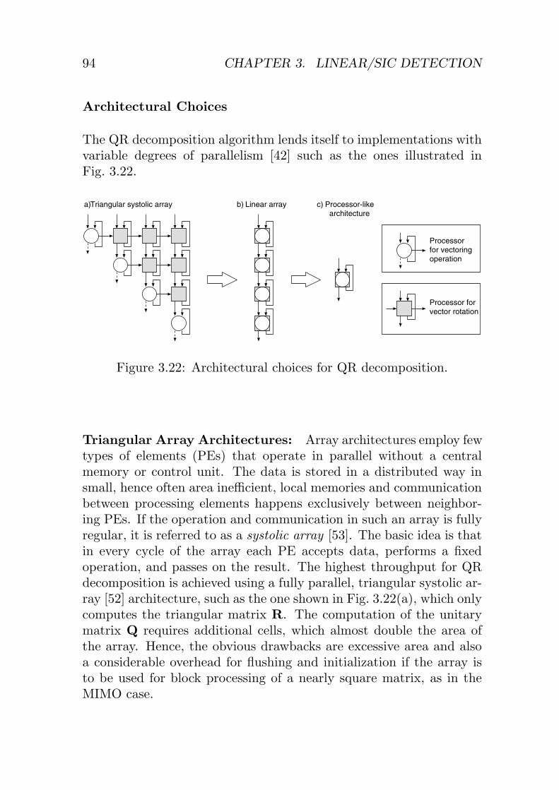
94 CHAPTER 3. LINEAR/SIC DETECTION
Architectural Choices
The QR decomposition algorithm lends itself to implementations withvariable degrees of parallelism [42] such as the ones illustrated inFig. 3.22.
Processor for vectoring operation
Processor for vector rotation
Processor-likearchitecture
Linear arrayTriangular systolic arraya) b) c)
Figure 3.22: Architectural choices for QR decomposition.
Triangular Array Architectures: Array architectures employ fewtypes of elements (PEs) that operate in parallel without a centralmemory or control unit. The data is stored in a distributed way insmall, hence often area inefficient, local memories and communicationbetween processing elements happens exclusively between neighbor-ing PEs. If the operation and communication in such an array is fullyregular, it is referred to as a systolic array [53]. The basic idea is thatin every cycle of the array each PE accepts data, performs a fixedoperation, and passes on the result. The highest throughput for QRdecomposition is achieved using a fully parallel, triangular systolic ar-ray [52] architecture, such as the one shown in Fig. 3.22(a), which onlycomputes the triangular matrix R. The computation of the unitarymatrix Q requires additional cells, which almost double the area ofthe array. Hence, the obvious drawbacks are excessive area and alsoa considerable overhead for flushing and initialization if the array isto be used for block processing of a nearly square matrix, as in theMIMO case.

3.3. VLSI IMPLEMENTATIONS 95
Linear Array Architectures: Linear array architectures with lessparallel processing [54], such as the one in Fig. 3.22(b), are a compro-mise between area and throughput. However, as opposed to triangulararrays, such linear array implementations with only local communica-tion achieve a lower resource utilization, typically only between 50%and 75%.
Processor-Like Architectures: Further resource sharing in lineararray architectures ultimately leads to the implementation of the QRalgorithm on a single, processor-like architecture (c.f. Fig. 3.22(c)),in which one or multiple arithmetic units are arranged around a cen-tral memory. The main advantages of such an arrangement, com-pared to array architectures, are flexibility, high resource utilization,more efficient memory structures, and the ability to exploit the po-tential in the QR algorithms to avoid operations with results that areknown a-priori. Hence, such a processor-like architecture should bepreferred over other architectures wherever it can meet throughputrequirements. As this is often the case for the MIMO systems underconsideration, we shall focus on the implementation of such structuresin the following.
Implementation of Vectoring and Vector Rotation
Two types of operations are required for the implementation of QR de-composition through Givens rotations: vectoring and vector rotation.Both operations can be implemented using conventional arithmetic orusing dedicated CORDIC circuits [55, 56]. A vast amount of litera-ture exists on the efficient circuit-level implementation of CORDICs.However, so far, a systematic exploration of the design-space, com-paring CORDIC implementations with conventional-arithmetic basedsolutions is still missing. Hence, we shall start by addressing this issuein the following:
CORDIC Based Implementation: The idea behind CORDICcircuits is to decompose the rotation of a vector by an angle φ into aseries of N subsequent clockwise or counter-clockwise micro rotations

96 CHAPTER 3. LINEAR/SIC DETECTION
according to(cosφ sinφ− sinφ cosφ
) (xy
)= γ
N∏i=1
(1 δi2−i
−δi2−i 1
) (xy
).
(3.60)
The coefficients δi of these micro rotations are chosen from ±1 insuch a way that φ =
∑Ni=1 δi atan(2−i) and γ is a scaling factor that
depends on N . For our subsequent discussion, this scaling can be ig-nored, as it can be decoupled from the actual vector rotation and weshall later only consider its impact on our conclusions. Each microrotation only involves shift and add operations and can thus be imple-mented efficiently in hardware. For the vectoring operation, a decisionis made after each micro rotation, whether the next micro rotationshould be clockwise (δi+1 = +1) or counter-clockwise (δi+1 = −1) inorder to null y. The result of the vectoring operation after N stepsis then the rotated vector with y close to zero and the correspondingrotation angle, encoded in the coefficients δi. These coefficients canthen be used to steer the micro rotations in the vector rotations ofthe corresponding Givens rotations.The block diagram of an iteratively decomposed CORDIC circuit,in which the N micro rotations are carried out sequentially over Ncycles, is shown in Fig. 3.23(a). The arithmetic part consists of twoadders/subtracters, two barrel shifters, and of a simple comparatorfor the vectoring operation. For simplicity, the control overhead andthe multiplexers to load new vectors into the registers are not shownin the figure. Performing K-fold loop unrolling [57] on the circuitin Fig. 3.23(a) yields the circuit in Fig. 3.23(b), which performs thesame operation in N/K cycles, but also requires the instantiationof K ALUs. Unfortunately, the unrolled circuit also has a longercritical path through K ALUs instead of through one ALU. Only thebarrel shifter becomes simpler in the unrolled architecture and evencompletely disappears for K = N . Still, one would initially expectonly marginal throughput gains and a significantly higher AT -productfor the unrolled architecture, compared to the decomposed circuit inFig. 3.23(a).Despite these not too favorable predictions, we shall continue by com-paring actual implementation results of decomposed and partially or

3.3. VLSI IMPLEMENTATIONS 97
+/-
>>
+/-
>>
>0
x y
δi
Rotationa)
x y
Rot.
Rot.
Rot.
b)
K≤
N
ALU 1
ALU 2
ALU K
Figure 3.23: Block diagram of an iteratively decomposed CORDIC(a) and a (partially) unrolled CORDIC (b).
fully unrolled CORDIC architectures. To this end, logic synthesis isperformed with different optimization goals between minimum areaand minimum delay and the results are plotted in the AT diagramin Fig. 3.24. The time needed to complete a vector rotation (withN = 8) is shown on the horizontal axis13 and the area of the circuitis given on the vertical axis. The vectoring and rotation modes areconsidered separately in the chart and both are analyzed for an itera-tively decomposed and for a fully unrolled (K = N) architecture. Forthe vectoring operation, the chart shows the expected behavior, indi-cating that the unrolled architecture must be associated with a large
13The associated cycle time is given by the time required for the operation,divided by the number of cycles, required for the operation.

98 CHAPTER 3. LINEAR/SIC DETECTION
area penalty, but ultimately enables the highest throughput. The ro-tation mode CORDIC also shows a large area for the minimum-delayimplementation. However, the area drops sharply with only a minorincrease in delay. Surprisingly, the unrolled architecture, in the corre-sponding minimum-area limit, almost matches the characteristics ofthe decomposed architecture in the minimum-delay limit, but requiresa much lower clock frequency. The reason for this favorable behaviorlies in the fact that a ripple-carry adder can be used for the unrolledarchitecture with area-only optimization. With the regular carry pro-file of this type of adder, the delays of the subsequent ALUs do notadd up [58]. Instead, only the adder in the first ALU exhibits its full(worst case) delay, while the subsequent ALUs contribute much lessto the overall critical path. Unfortunately, one can not leverage thisadvantage in the vectoring mode. There, the longest path in eachstage is between the input that determines the rotation direction ofthe micro rotation and the output (taken from the most significantbit) that specifies the rotation direction for the next micro rotation.Hence, the full worst-case delays of the cascaded ALUs add up andthe cycle time grows almost proportional to the number of unrolledmicro rotations.
Complex Multiplier Implementation: We start by reconsider-ing the problem of implementing the vector rotation: An alternativeto CORDIC circuits is to perform the vector rotation in (3.60) in thecomplex plane by using conventional complex-valued multipliers withinputs x+ jy and with the complex phasor cosφ− j sinφ. The corre-sponding circuit is comprised of either four real-valued multipliers andtwo adders, or of only three real-valued multipliers and five adders.While implementations with only three multipliers provide a smallarea advantage, they perform much worse in terms of delay, leadingto an overall larger AT -product. Hence, in the following, we shallfocus on circuits which are comprised of four real-valued multipliers.For designspace exploration consider a single-cycle isomorphic archi-tecture and a two-cycle architecture with only two real-valued multi-pliers using resource sharing. The corresponding area/delay tradeoffcurves are also given in Fig. 3.24. From the chart, one can observethat the multiplier architectures extend the design space covered by

3.3. VLSI IMPLEMENTATIONS 99
the CORDIC circuits, to significantly lower delays, while the opti-mization for speed also leads to better AT -products. An additionaladvantage of the multiplier architectures is that excessive iterative de-composition is not necessary in order to reduce area so that efficientimplementations can still operate at low to moderate clock rates.
Figure 3.24: Design space exploration of circuit implementations forvectoring and vector rotation for the implementation of Givens rota-tions.
The difficulty in using multiplier-based circuits for the vector rotationlies in the generation of the corresponding complex rotation coeffi-cients cosφ− j sinφ in the associated vectoring operations. The mostobvious approach is to also perform the vectoring on [ x y ]T usingconventional arithmetic. The coefficients for the subsequent rotationsare then immediately given by
cosφ =x√
x2 + y2and sinφ =
y√x2 + y2
. (3.61)

100 CHAPTER 3. LINEAR/SIC DETECTION
Unfortunately, the squaring, the divisions and especially the squareroot are associated with high implementation costs. Therefore, weshall resort to the use of the vectoring CORDICs and we shall ex-plore suitable extensions that allow to obtain the coefficients for acomplex-valued-multiplier based rotation unit from the outputs ofthat CORDIC. The CORDIC can easily be modified to output φ in-stead of the corresponding directions δi of the micro rotations [59]. Aseparate unit can then compute e−jφ from φ as shown in Fig. 3.25(a).This problem is well known in the field of direct digital synthesis(DDS) and a number of circuits have been proposed using for examplelook-up tables or approximations of the trigonometric functions [60].A particularly appealing scheme, which even avoids the translation ofthe δi into φ, is based on a simple rotation-mode CORDIC (withoutscaling correction). In the architectures shown in Fig. 3.25(b), thisadditional rotation mode CORDIC starts from [ 1/γ 0 ]T and fol-lows the micro rotations performed in the vectoring CORDIC. AfterN iterations, its outputs correspond to the desired complex-valuedcoefficient for multiplier based vector rotation unit(s). In terms of sil-
VectoringCORDIC
DDS
Com
pute
Pha
se
x y
φ
e−jφ
VectoringCORDIC
RotationCORDIC
1/γ 0x y
e−jφ
δ
a) b)
Figure 3.25: CORDIC circuits for vectoring operation that also obtaina phasor for rotation with complex multipliers.
icon area, the extended vectoring CORDIC is roughly twice as largeas a standard vectoring CORDIC. However, since the critical path isstill determined by the vectoring unit, the timing remains unchanged.
Comparison: Purely CORDIC-based implementations offer the high-est potential for resource sharing to minimize silicon area, because thesame circuit can be reused for vectoring and rotation operations. As

3.3. VLSI IMPLEMENTATIONS 101
both operations are implemented using CORDIC circuits, they in-terface seamlessly with each other, requiring no additional hardwareoverhead. More on the negative side, the best hardware efficiency (i.e.,the lowest AT -product) and high throughput at low area can only beachieved with excessive iterative decomposition of the CORDIC cir-cuit, which leads to extremely high clock rates.
Conventional-arithmetic based architectures must still use CORDICsfor vectoring and require additional hardware to compute the coef-ficients for the vector rotation with complex-valued multipliers. Theadvantages over architectures that rely solely on CORDIC circuits arethe significantly shorter delays for vector rotation, which are achievedwith a better AT -product and at a lower clock frequency. Hence, themultiplier-based architecture is more suitable for achieving the highestperformance.
Numerical Considerations
It has been claimed in Sec. 3.2.2 that QR decomposition is less criticalin terms of its fixed-point requirements compared to direct matrixinversion algorithms. The subsequent analysis serves to underminethis claim. It summarizes the corresponding important considerationsin the implementation of QR decomposition for MIMO detection.
Input Normalization: For the fixed-point analysis, we start againwith a dynamically scaled channel matrix H = αH, where α is chosenaccording to the scheme that has also been used for the fixed-pointanalysis of the Riccati recursion algorithm in Sec. 3.3.1. This blockfloating-point normalization ensures that
∣∣∣��{Hi,j}∣∣∣ ≤ 1.
Dynamic Range Requirements: The dynamic range requirementsfor the entries of the matrices Q and R are computed first, becausethey also bound the dynamic range of entries of all intermediate vari-ables in the algorithm and thus determine the number of requiredinteger bits. The matrix Q is unitary by design, so that all its entriesQi,j are constrained to |Qi,j | ≤ 1. The dynamic range of the real and

102 CHAPTER 3. LINEAR/SIC DETECTION
imaginary parts of the entries of R is given by
|��{Ri,j}| <√2MR +MTσ, (3.62)
where MTσ is small enough to be ignored for reasonable SNRs14.
Complexity/Performance Tradeoffs: Given the dynamic rangerequirements of the QR algorithm, one can determine the remainingfixed-point design parameters. To avoid an explosion of the designspace when trying to jointly optimize wordlengths across all degreesof freedom, a hierarchical approach is chosen, where the parameterwith the greatest influence on the overall circuit complexity is consid-ered first. In the case of an architecture that is based on CORDICcircuits for both vectoring and vector rotation operations, this mostcritical parameter is the number of micro rotations N . The impactof the choice of N on the overall bit-error rate is evaluated throughnumerical simulations in which all other variables are still kept infloating-point format. Fig. 3.26 shows BER simulation results forzero-forcing detection using QR decomposition in a 4×4 system with16-QAM modulation for different choices of N . In the example, close-to floating-point performance is already achieved for N = 7.
Having determined an appropriate choice for the required number ofmicro rotations N , one can now analytically derive accuracy require-ments for the individual vectoring and rotation operations. To thisend, we use a result from [61], which states that the error at the outputof a CORDIC15 can be approximated by
E{MSE(N)} ≈ 19
(arctan
(2−N
))2. (3.63)
The number of fractional bits at the output of the CORDIC cannow be chosen sufficiently large to ensure that the correspondingadditional quantization noise remains well below E{MSE(N)}. ForCORDICs that use truncation at the output it is found that at least
14For zero-forcing, σ = 0.15It is assumed that the inputs are uniformly distributed between -1 and +1.
For our case, this is a pessimistic assumption, but is sufficient for establishingconservative implementation guidelines.

3.3. VLSI IMPLEMENTATIONS 103
Figure 3.26: QR-based ZF performance in a 4×4 system with 16-QAMmodulation for different number of CORDIC iterations (5’000 channelrealizations).
�N − log2(1/6)/2� fractional bits must be reserved, while with round-ing, this minimum reduces by one bit to �N − log2(4/6)/2�. Withinthe CORDIC circuit itself, log2 N additional bits must be used forthe implementation of the accumulator to keep the aggregate quanti-zation error of the N micro rotations below the output quantizationnoise. Finally, the width of the constant scaling coefficient γ needsto be determined. Simulation results show that a representation withsix bits (γ ≈ 0.609375) is sufficient for most purposes and is easy toimplement in hardware with only two adders, using the correspondingcanonical-signed digit representation [59].
Fully Decomposed QR Processor (Architecture I)
Our first VLSI architecture of a QR processor for MIMO detectionis targeted towards systems in which preprocessing latency is onlyconstrained by the coherence time of a slowly fading channel. Hence,the hardware that executes the optimized QR algorithms presented inSec. 3.2.2 can be optimized for low area.

104 CHAPTER 3. LINEAR/SIC DETECTION
Architecture: The high-level VLSI architecture of such an area-optimized QR processor can be kept extremely simple as illustratedin the block diagram in Fig. 3.27. The real and imaginary parts ofthe matrices H and I are initially stored in a register file (i.e., afast memory with separate read and write ports) and are modifiedby the arithmetic unit throughout the QR decomposition algorithmso that the memory in the end contains R and Q. The processor iscontrolled by the Load/QR control unit, which fetches two real-valuedentries16 from the memory and starts the corresponding vectoring orrotation operation. The minimum-area requirement is best met byemploying only a single real-valued CORDIC circuit that performsboth vectoring and rotation operations. The area of this CORDICcircuit is minimized by using full iterative decomposition. Hence, Ncycles are required to complete vectoring or vector rotation operations.During this time, the results of the previous operation can be writtenback to the memory by the writeback unit and the next operands canalready be fetched. For a reasonably large number of micro rotations(7-10 is typically required for sufficient accuracy) the CORDIC canbe kept busy even with a single-port memory, where read and writeoperations must be carried out sequentially.
Implementation Results: The reference implementation exampleis a preprocessing unit for BS-based ZF detection or for Sphere De-coding in a 4× 4 MIMO system. Both detection schemes require astraightforward QR decomposition of the estimated channel matrixH, which can be performed efficiently as described in Sec. 3.2.2. Weassume an SNR operating range of up to 30 dB, based on which thenumber of micro rotations is chosen conservatively to be N = 8. Thecorresponding input and output word lengths of the CORDIC are 13bits, which are comprised of one sign bit, two integer bits and 10fractional bits to match the accuracy achieved by the N = 8 microrotations. For the accumulators in the CORDIC, three additionalfractional bits have been allocated.
The CORDIC is implemented using full and partial iterative decom-position. In the fully decomposed design (K = 1), one micro ro-
16A real-valued entry can be the real or imaginary part of a complex-valuednumber.

3.3. VLSI IMPLEMENTATIONS 105
0 1
Writebackcontrol
Load/QRcontrol
Vectoring/rotation
CORDIC
REQ/ACK
H,I / Q,R Memory(register file)read port write port
vec./rot.
ADDR
Figure 3.27: Block diagram of the area optimized QR processor.
tation is carried out in each clock cycle. An additional cycle is re-served for the scaling of the output of the CORDIC with γ. Thetotal number of cycles required for the QR decomposition is givenby (N +1)(CVec(ZF)+CGR(ZF)), where CVec(ZF) and CGR(ZF) canbe obtained from (3.37) and (3.38), respectively. In the partially de-composed design, two micro rotations are combined to a single cycle(K = 2). The result is a lower clock rate but the number of cyclesalso reduces to (N/2 + 1)(CVec(ZF) + CGR(ZF)).
The implementation results (after synthesis) are summarized in thefirst three columns of Tbl. 3.4. In all implementations, the memoryconsumes an equivalent of 3.9K GEs, which constitutes a significantportion of the overall silicon area. The speed-optimized fully and par-tially decomposed designs provide comparable preprocessing delays,however, with the decomposed CORDIC, a much lower clock rate isrequired. The optimization for low area leads to a disproportionateincrease in cycle time so that it yields no advantage in terms of theoverall AT -product compared to the implementations that were opti-mized for speed.
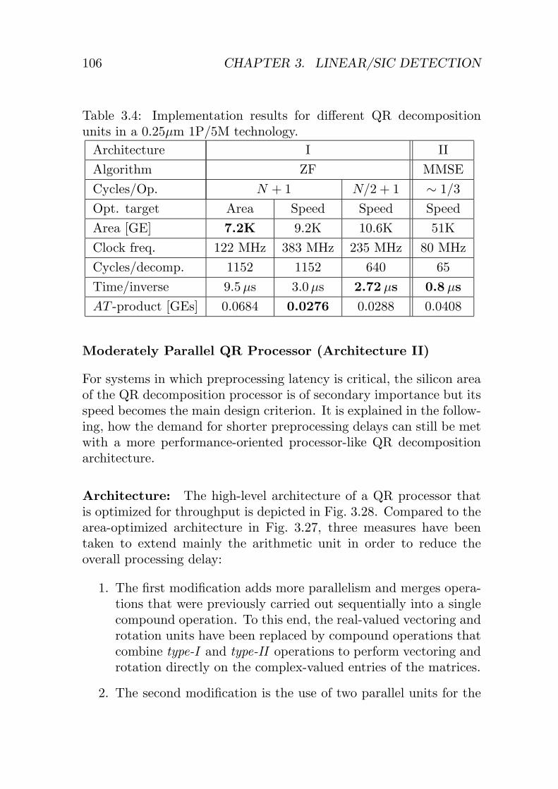
106 CHAPTER 3. LINEAR/SIC DETECTION
Table 3.4: Implementation results for different QR decompositionunits in a 0.25µm 1P/5M technology.Architecture I IIAlgorithm ZF MMSECycles/Op. N + 1 N/2 + 1 ∼ 1/3Opt. target Area Speed Speed SpeedArea [GE] 7.2K 9.2K 10.6K 51KClock freq. 122 MHz 383 MHz 235 MHz 80 MHzCycles/decomp. 1152 1152 640 65Time/inverse 9.5µs 3.0µs 2.72 µs 0.8 µsAT -product [GEs] 0.0684 0.0276 0.0288 0.0408
Moderately Parallel QR Processor (Architecture II)
For systems in which preprocessing latency is critical, the silicon areaof the QR decomposition processor is of secondary importance but itsspeed becomes the main design criterion. It is explained in the follow-ing, how the demand for shorter preprocessing delays can still be metwith a more performance-oriented processor-like QR decompositionarchitecture.
Architecture: The high-level architecture of a QR processor thatis optimized for throughput is depicted in Fig. 3.28. Compared to thearea-optimized architecture in Fig. 3.27, three measures have beentaken to extend mainly the arithmetic unit in order to reduce theoverall processing delay:
1. The first modification adds more parallelism and merges opera-tions that were previously carried out sequentially into a singlecompound operation. To this end, the real-valued vectoring androtation units have been replaced by compound operations thatcombine type-I and type-II operations to perform vectoring androtation directly on the complex-valued entries of the matrices.
2. The second modification is the use of two parallel units for the

3.3. VLSI IMPLEMENTATIONS 107
H,I
/ Q,R
Mem
ory
(reg
iste
r fil
e w
ith s
epar
ate
read
and
writ
e po
rts
for
even
and
odd
row
s)
read
por
tw
rite
port
Com
plex
vect
orin
gC
OR
DIC
Load
/QR
cont
rol
Com
plex
vect
orro
tatio
n
Writ
ebac
kco
ntro
l
01
MT
σ
0
Vec
torin
gV
ecto
rro
tatio
n
Vec
torin
gV
ecto
rro
tatio
nV
ecto
rro
tatio
n
Mem
ory
bypa
ss
e−
jφ
e−
jψ
Figure 3.28: Block diagram of the low-latency QR processor.

108 CHAPTER 3. LINEAR/SIC DETECTION
vectoring and rotation operation. The main advantage is thatdata dependencies allow hiding each of the few vectoring op-erations behind multiple rotation operations, as illustrated inFig. 3.28. Hence, vectoring can be optimized for area through it-erative decomposition without affecting the overall performance17.
3. The last modification is the choice of fast, single-cycle, complex-valued multipliers to implement the concatenated type-I andtype-II vector rotations with the shortest possible delay.
The main issue with such a modified architecture is the available mem-ory access bandwidth. For the single-cycle complex-valued vector ro-tation, two read accesses and two write accesses are required in eachcycle to load two new complex-valued operands and to write back thetwo complex-valued results from the previous operation. In order tomeet this requirement, a more sophisticated memory architecture isneeded. It is based on the fact that with the complex-valued vector-ing and rotation operations all operands are always complex numberswhich can now be stored in a single, wider data word. Moreover, onecan exploit that parallel memory accesses are always performed on aneven and an odd row of the matrices. Hence, the access bandwidthbottleneck can be resolved by splitting the memories into two parallelmemories, one for the even and one for the odd rows. Finally, forvectoring only few additional memory access cycles are required sincemost of the associated operands can be taken from a small cache inthe load unit which keeps copies of the corresponding outputs of thevector rotation unit to bypass the memory bottleneck.
Implementation Results: The reference implementation of thissecond architecture performs QR preprocessing for MMSE linear de-tection and SIC in an IEEE 802.11n-like MIMO receiver ASIC [62].The system under consideration is a packet-based MIMO-OFDM sys-tem in which preprocessing needs to be performed for up to 64 tones18
17Performance only starts to degrade, when the required number of cycles forvectoring exceeds the number of rotation operations that have to be carried outin parallel.
18Only 52 of the 64 tones are actually used for data. The remaining tones arereserved for pilots and guard intervals.

3.3. VLSI IMPLEMENTATIONS 109
CC
C···
CC
C···
CC
C···
R0
0···
0R
0···
CC
C···
CC
C···
RC
C···
00
0···
0R
0···
CC
C···
RC
C···
0C
C···
0C
C···
0R
0···
RC
C···
0C
C···
0C
C···
0C
C···
0R
0···
Vec
torin
g
Rot
atio
n
cycl
es
Figure 3.29: Illustration of the parallel processing of vectoring androtation operations in MMSE QR decomposition.

110 CHAPTER 3. LINEAR/SIC DETECTION
under tight latency constraints. MMSE detection requires QR de-composition of the augmented channel matrix H = [HH ;
√MTσI]H
which can be performed efficiently on a processor-like architecture ac-cording to the algorithm that has been described in Sec. 3.2.2. BERsimulations show that in a CORDIC-based implementation N = 9 mi-cro rotations cover the systems SNR operating range of up to 30 dBwith close-to floating-point performance. Herewith, the correspond-ing wordlength for the inputs and outputs of the vectoring and vectorrotation units (and of the memories) are found to be 14 bits, which arecomprised of one sign bit, two integer bits and 11 fractional bits. Therotation coefficients of the complex-multiplier based rotation unitsalso use 11 fractional bits to match the accuracy of the N = 9 microrotations.Due to data dependencies, it is more difficult to give an exact ana-lytical expression for the number of cycles in the moderately parallel,processor-like architecture, compared to the fully decomposed archi-tecture. However, a close-to accurate estimate is obtained from thenumber of vector rotation operations CRot(MMSE), which is givenby (3.44). With the composite vector rotation unit, three of these op-erations are performed in one cycle, and the additional vectoring oper-ations are almost all performed in parallel in the background. Hence,the total number of cycles for the QR decomposition for MMSE de-tection is approximately given by CRot(MMSE)/3.Implementation results after synthesis for the described design aregiven in the third column of Tbl. 3.4. Despite the fact that the QRdecomposition for MMSE detection requires roughly 50% more oper-ations compared to QR decomposition for ZF detection, the designachieves a much shorter preprocessing latency than the fully decom-posed architectures. However, at the same time, it consumes more sil-icon area. For a fair comparison of the AT -products of architectures Iand II, the AT -product of the ZF detectors must be scaled by a factorof 1.5, which corresponds to the increase in the number of operationswhen performing QR decomposition for MMSE detection instead ofZF. Notably, the scaled AT -product of the area-optimized first archi-tecture in column two of Tbl. 3.4 now almost matches the AT -productof the latency-optimized second architecture (1.5 × 0.0276 = 0.0414vs. 0.0408, respectively).

Chapter 4
Implementation ofExhaustive Search ML
Exhaustive search detection refers to the straight forward implemen-tation of the ML criterion which is given by
s = arg mins∈OMT
‖y −Hs‖2. (4.1)
The basic idea is to explicitly compute the Euclidean distance betweenthe received point y and all possible (noiseless) received symbols Hswith s ∈ OMT in order to find the minimum by explicitly comparingthe results.
Complexity Advantages with Exhaustive Search ML
Despite the, at first sight, prohibitive computational complexity, whichgrows exponentially with the rate of the communication system, BERperformance considerations strongly advocate the use of ML detectionin order to be able to exploit the full diversity of the MIMO channel.Surprisingly, we shall see that even from an implementation point ofview, one can make a case for the use of an exhaustive search MLdecoder, provided that the rate is not too high. In particular, the fol-
111

112 CHAPTER 4. EXHAUSTIVE SEARCH ML
lowing properties of an exhaustive search ML detector are favorablefor a VLSI implementation:
� The algorithm has a very high regularity and only few datadependencies allow for a significant degree of parallel processing.
� No costly operations, such as divisions or square roots, are re-quired.
� Due to the relaxed numerical requirements of (4.1), silicon areaof arithmetic components and the amount of memory storagecan be kept low.
� Simple, but lossless (in terms of BER performance) algorithmictransformations lead to expressions that reveal a large number ofcommon terms which can be precomputed. Such optimizationsessentially allow to partially mitigate the impact of the exponen-tial complexity increase with rate by reducing the scaling factorin front of the exponential term in the complexity expression.
4.1 High-Level Architecture
A key concern in the high-level architectural design of an exhaustivesearch detector is the partitioning between channel-rate preprocessingand symbol-rate detection. It is assumed in the following that thetiming requirements for the channel-rate processing are only governedby the channel coherence time, which is assumed to be large comparedto the symbol-rate timing. Hence, significant resource sharing anditerative decomposition can be applied to reduce the silicon complexityof the preprocessing, while highly parallel solutions are of interest forthe detection stage to attain high-throughputs. These assumptionsgovern our subsequent architectural choices and optimizations.
Complexity Considerations
Before discussing two high-level architectures for an exhaustive searchML detector, three partially contradicting optimization goals are set

4.1. HIGH-LEVEL ARCHITECTURE 113
out which need to be balanced in order to achieve an overall efficientdesign:
� The aim is to move as many operations as possible into thepreprocessing in order to reduce the computational burden onthe high-throughput part of the detector.
� Complexity (area and delay) is not only determined by the num-ber of operations but also by their relative hardware implemen-tation cost. Consequentlt, it is desirable to move costly op-erations into the channel-rate preprocessing, even if this maycome at the expense of additional, less complex operations inthe symbol-rate processing.
� Finally, the results of the preprocessing need to be stored. Pre-computing more partial results reduces the silicon complexity ofthe data path but also increases memory storage requirements.
4.1.1 Architecture I
The block diagram of the implementation strategy reported in [63, 64]is shown in Fig. 4.1. The basic idea is to precompute all possiblecandidate vector symbols Hs at channel rate and to store them in acache. Symbol-rate detection then fetches the precomputed candidatesymbols from that cache, subtracts each of them from the receivedvector y, computes the (approximated) vector-norm of the result andfinds the minimum.
Complexity
A complexity analysis of this first architecture reveals three majordisadvantages:
1. The computation of the vector-norm at symbol rate is a costlyoperation1 which requires significant silicon area. Achievinghigher throughput with parallel processing of multiple candidate
1Note that complexity can be reduced by using approximations for the �2-normat the expense of BER performance.

114 CHAPTER 4. EXHAUSTIVE SEARCH ML
Hs−CacheH
y arg min||y − Hs||2
Precompute
Hs
Figure 4.1: High-level architecture for an exhaustive search ML de-tector as proposed in [63].
symbols in the detection stage therefore entails the replicationof costly operations and hence leads to a rapid increase in siliconcomplexity.
2. A large cache is required to store the |O|MT MR-dimensionalreference vectors Hs that have been computed during channel-rate preprocessing. The result is a significant contribution ofthe cache memory to the overall area of the detector.
3. Considerable access bandwidth to the Hs-Cache is needed tofetch the reference vectors at symbol rate. This can only beachieved through the use of wide, but shallow memories or throughcustom multiport memories. However, both suffer from a lowarea efficiency.
From the above discussion it can be concluded that the architecturein Fig. 4.1 does not meet the previously defined complexity consider-ations for a high throughput VLSI architecture.
4.1.2 Architecture II
In order to obtain a more efficient high-level architecture [8] the com-pact form of the ML criterion in (4.1) is expanded in the followingway
s = arg mins∈OMT
(‖Hs‖2 − 2�
{(yHH)s
}+ c
), (4.2)

4.1. HIGH-LEVEL ARCHITECTURE 115
where c = ‖y‖2. As opposed to the first architecture, channel-rateprocessing now computes the squared vector-norms z(s) = ‖Hs‖2 ofthe reference vectors and stores them in the cache. For each receivedvector, the symbol-rate processing first obtains y = yHH which isthen used to compute d(s) = z(s)− 2�{ys} for all s ∈ OMT . As theremaining term c is a constant with respect to s it can be ignored andfinding the minimum among the d(s) yields the ML solution. Thecorresponding block diagram of this second architecture is shown inFig. 4.2.
||Hs||2-Cache
H
y arg miny = yHH 2�{ys}s ∈ OMT
Precompute
||Hs||2
Figure 4.2: Optimized architecture for an exhaustive search detector.
Complexity
For the complexity analysis, the channel-rate processing and the cachememory that connects it to the symbol-rate processingare consideredfirst. The number of computations in this part of the design clearlyincreases compared to the first architecture. However, if it can beassumed that the channel changes only slowly, significant resourcesharing can be applied to keep the overall silicon complexity low. Moreimportantly, only a scalar value has to be retained in the cache foreach reference vector which yields a considerable reduction in the sizeof the cache and also reduces the required access bandwidth.The complexity of the symbol-rate processing is governed by the com-putation of y and 2�{ys}. The former requires costly full complex-valued multiplications, however, it is not affected by the exponentialcomplexity increase with rate. In fact, the number of complex mul-tiplications only grows proportionally to MRMT and is comparable

116 CHAPTER 4. EXHAUSTIVE SEARCH ML
to a MM-based linear detector, however, with significantly relaxeddynamic range requirements for the fixed-point representation. Thehighest number of operations in the symbol-rate processing is requiredfor the computation of 2�{ys} for all possible candidate vector sym-bols s ∈ OMT . However, as the entries of s are all chosen from thesmall set of constellation points (si ∈ O), highly optimized, hencearea efficient, constant-coefficient multipliers can be used. Therefore,as opposed to the detection stage of the first architecture, no costlyoperations are associated with the exponential complexity increasewith rate. Hence, the second design is expected to be better scalableand to yield a lower silicon complexity.
4.2 Complexity Reduction
Starting from the optimized architecture in Fig. 4.2, it is shown inthe following how the silicon complexity of the decoder can be furtherreduced by exploiting properties of the modulation scheme and byidentifying common or redundant terms in the computation that caneither be shared or dropped. As in the optimization of the high-levelarchitecture, the focus is thereby on reducing the number of costlyoperations that are affected by the exponential complexity increasewith rate, noting that such transformations may come at the expenseof additional, but less costly operations.
Preprocessing and Cache: The relaxed timing requirements forthe channel-rate processing leave significant room for complexity re-duction through extensive resource sharing. Nevertheless, complexityreduction is still of interest to reduce power consumption and to sup-port communication systems, in which channel-rate processing latencyis a concern.The straightforward implementation of z(s) = ‖Hs‖2 requires thecomputation of a large number �2-norms. A more efficient approachis again achieved by rewriting the expression for z(s) in a more explicitaccording to
z(s) = sHLs with L =(HHH
). (4.3)
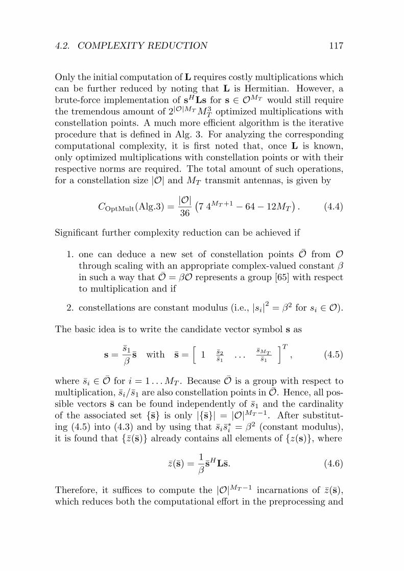
4.2. COMPLEXITY REDUCTION 117
Only the initial computation of L requires costly multiplications whichcan be further reduced by noting that L is Hermitian. However, abrute-force implementation of sHLs for s ∈ OMT would still requirethe tremendous amount of 2|O|MT M3
T optimized multiplications withconstellation points. A much more efficient algorithm is the iterativeprocedure that is defined in Alg. 3. For analyzing the correspondingcomputational complexity, it is first noted that, once L is known,only optimized multiplications with constellation points or with theirrespective norms are required. The total amount of such operations,for a constellation size |O| and MT transmit antennas, is given by
COptMult(Alg.3) =|O|36
(7 4MT+1 − 64− 12MT
). (4.4)
Significant further complexity reduction can be achieved if
1. one can deduce a new set of constellation points O from Othrough scaling with an appropriate complex-valued constant βin such a way that O = βO represents a group [65] with respectto multiplication and if
2. constellations are constant modulus (i.e., |si|2 = β2 for si ∈ O).
The basic idea is to write the candidate vector symbol s as
s =s1βs with s =
[1 s2
s1. . .
sMT
s1
]T
, (4.5)
where si ∈ O for i = 1 . . .MT . Because O is a group with respect tomultiplication, si/s1 are also constellation points in O. Hence, all pos-sible vectors s can be found independently of s1 and the cardinalityof the associated set {s} is only |{s}| = |O|MT −1. After substitut-ing (4.5) into (4.3) and by using that sis
∗i = β2 (constant modulus),
it is found that {z(s)} already contains all elements of {z(s)}, where
z(s) =1βsHLs. (4.6)
Therefore, it suffices to compute the |O|MT −1 incarnations of z(s),which reduces both the computational effort in the preprocessing and
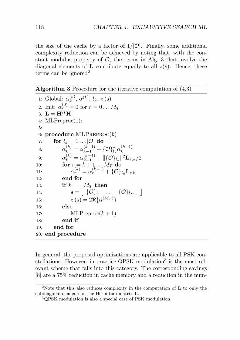
118 CHAPTER 4. EXHAUSTIVE SEARCH ML
the size of the cache by a factor of 1/|O|. Finally, some additionalcomplexity reduction can be achieved by noting that, with the con-stant modulus property of O, the terms in Alg. 3 that involve thediagonal elements of L contribute equally to all z(s). Hence, theseterms can be ignored2.
Algorithm 3 Procedure for the iterative computation of (4.3)
1: Global: α(k)k , α(k), lk, z (s)
2: Init: α(0)r = 0 for r = 0 . . .MT
3: L = HHH4: MLPreproc(1);5:
6: procedure MLPreproc(k)7: for lk = 1 . . . |O| do8: α
(k)k = α
(k−1)k−1 + {O}∗lkα
(k−1)k
9: α(k)k = α
(k−1)k−1 + ‖{O}lk‖2Lk,k/2
10: for r = k + 1 . . .MT do11: α
(k)r = α
(k−1)r + {O}lkLr,k
12: end for13: if k ==MT then14: s =
[{O}l1 . . . {O}lMT
]15: z (s) = 2�{α(MT )}16: else17: MLPreproc(k + 1)18: end if19: end for20: end procedure
In general, the proposed optimizations are applicable to all PSK con-stellations. However, in practice QPSK modulation3 is the most rel-evant scheme that falls into this category. The corresponding savings[8] are a 75% reduction in cache memory and a reduction in the num-
2Note that this also reduces complexity in the computation of L to only thesubdiagonal elements of the Hermitian matrix L.
3QPSK modulation is also a special case of PSK modulation.

4.2. COMPLEXITY REDUCTION 119
ber of operations for the channel-rate preprocessing to
COptMult(Alg.3,QPSK) =494MT − 1
3MT −
49. (4.7)
Symbol-Rate Processing: The matrix-vector product for the com-putation of y (cf. Sec. 3.1.1) only allows for the most basic architec-tural transformations to trade area for processing delay. However, thispart of the design is neither the limiting factor in terms of throughput,nor the dominant part in terms of silicon area. In the following, weshall therefore concentrate on the much more critical remaining partsof the symbol-rate processing. These parts can be decomposed fur-ther into the computation of p(s) = ys and into finding the minimumamong all z(s)− 2�{p(s)} for s ∈ OMT .Alg. 4 describes the efficient computation of p(s). The procedure canbe realized with a single multiplier which is optimized for multiplica-tions with constellation points.
Algorithm 4 Procedure for the iterative computation of p(s)
1: Global: α(k), lk2: Init: α(0) = 03: ComputeP(1);4:
5: procedure ComputeP(k)6: for lk = 1 . . . |O| do7: α(k) = α(k−1) + {O}lk yk
8: if k ==MT then9: s =
[{O}l1 . . . {O}lMT
]10: p(s) = α(k)
11: else12: ComputeP(k + 1)13: end if14: end for15: end procedure
The drawback of such a fully decomposed architecture is a very lowthroughput because a large number of cycles is needed for the compu-

120 CHAPTER 4. EXHAUSTIVE SEARCH ML
tation. At the same time, little is gained in terms of silicon area overa more parallel approach since each iteration has only a low imple-mentation complexity. A better solution associates the computationof p(s) with a tree and assigns an optimized multiplier and an adderto each level of that tree (i.e., to each iteration). Now, one p(s) canbe computed in each cycle, where each s ∈ OMT is associated witha path from the root to a leaf. In order to increase throughput, onecan simply start to expand the D lower levels of the tree to compute|O|D incarnations of p(s) in parallel, as illustrated in Fig. 4.3. In theexample for MT = 3 with BPSK modulation, four p(s) are computedat a time by expanding D = 2 levels of the tree.
{O}1{O}1
{O}1{O}1
{O}1{O}1
0
y1
{O}l1
y2
y3
Cycle 1 Cycle 2p(s)
Figure 4.3: Architecture to compute all incarnations of p(s) forMT = 3 with BPSK modulation in two cycles.
However, the throughput advantage of such an expanded-tree archi-tecture can only be leveraged if one can continue to process the resultsin parallel. The main limitation is thereby the access bandwidth tothe cache that is required to fetch the |O|D corresponding z(s) in eachcycle for the computation of the decision parameters z(s)− 2�{p(s)}.In order to alleviate this bottleneck, it is shown how for PSK con-stellations a higher number of vector symbols can be processed in

4.3. IMPLEMENTATION RESULTS 121
parallel with no increase in the required cache access bandwidth andwith only a moderate increase in silicon area. For this purpose, thedecision criterion is first written as a function of s1 and s accordingto
arg mins1,s
(z (s)− 2�{s1p (s)}) . (4.8)
Because s1 = 1, the first stage of the logic, shown in Fig. 4.3, whichcomputes p(s) can be removed and the number of cycles to compute allpossible incarnations reduces by a factor of |O|. At the same time, |O|decision criteria can be computed in parallel for each p(s) with onlya single access to the cache memory to fetch the corresponding z(s).Finding the ML solution now corresponds to a two-step process: Thelocal minima with respect to s1 around each s are found first, followedby finding the global minimum among these local minima. For findingthe global minimum, explicit computation of the decision criteria andtheir comparison cannot be avoided. However, for a given s, s1 canbe determined analytically based on the phase of p(s) according to
s1 = arg mins1∈O
(arc s1 + arc p (s)) . (4.9)
In practice, (4.9) can be implemented without the use of transcen-dental functions by introducing suitable decision boundaries. Theseboundaries are defined by the quadrant in which p(s) is located andthrough simple relations between the absolute values of the real andimaginary parts of p(s). An illustration of the corresponding circuitfor QPSK modulation can be found in [8].
4.3 Implementation Results
To provide reference for the true silicon complexity of exhaustivesearch ML detection, actual implementation results of the ML-APPdetector in [64] and of our own implementation of a hard-decision ex-haustive search ML detector are listed in Tbl. 4.1. The ML-APP de-sign is based on Arch. I and implementation results are for a 0.18µmCMOS process. The circuit delivers soft outputs for a subsequentchannel decoder as approximate log-likelihood ratios (LLRs). Our

122 CHAPTER 4. EXHAUSTIVE SEARCH ML
reference designs for the optimized Arch. II deliver hard decisions andcomplexity estimates are based on a 0.25µm technology.
Comparison of Exhaustive Search Arch. I and Arch. II:
A comparison of the silicon area, the throughput and the hardwareefficiency of the two architectures for different system configurationsin Tbl. 4.1 clearly illustrates the advantage of the optimized Arch. II.However, it should also be noted that only architecture one can deliversoft-outputs which can lead to a performance improvement of morethan 2.5 dB in coded systems. Clearly, the computation of the log-likelihood ratios is partially responsible for the larger silicon area ofthe ML-APP design according to Arch. I [64].
Complexity Scaling Behavior:
The complexity scaling behavior of the ML-APP design has been de-scribed in [64] and it has been concluded that the true silicon complex-ity grows extremely fast as rate increases. Hence, we shall focus on thescaling behavior of our optimized, low-complexity Arch. II: The designfor the lowest rate (R = 4) in Tbl. 4.1 exhibits the highest throughput.As the rate increases, the number of bits per vector symbol increaseslinearly, however the complexity increases exponentially. Hence, theoverall throughput decreases as ∼ R2−R if the same number of can-didate vector symbols are processed in each cycle. To partially regainsome of the original throughput, more candidate vector symbols canbe processed in parallel at the expense of additional area. However,throughput gain for moderately parallel architectures is significantlyhigher than the corresponding area increase. Consequently, the ef-ficiency of the decoder is improved as illustrated in Tbl. 4.1. Thereason for this behaviour is the overhead from the preprocessing and,for higher rates, the area of the cache whose size only depends on therate and is mostly independent4 of the number of symbols that are pro-cessed in parallel. The results suggest that the optimized Arch. II for
4More parallel processing also requires the cache to be split into multiple mem-ories, to allow for sufficient access bandwidth. This slightly increases the cachearea. However, the effect is negligible for the moderate amounts of parallel pro-cessing that are applied here.

4.3. IMPLEMENTATION RESULTS 123
QPSK modulation scales well for rates up to 8 bpcu and may even beapplied for systems with 12 bpcu. However, beyond this limit, the truesilicon complexity becomes prohibitive with today’s VLSI technologyand one needs to resort to other, reduced-complexity algorithms.

124 CHAPTER 4. EXHAUSTIVE SEARCH ML
Table
4.1:Complexity
ofexhaustive
searchMLdetection
implem
entedaccording
toarchitectures
oneand
two.Implem
entationresults
forarchitecture
oneinclude
computation
ofsoft
outputsand
aretaken
from[64].
SystemRate
RThroughput
Area
#ofsconsidered
Efficiency
configuration[bpcu]
[GE]
inparallel
[Mbps/K
GE]
Architecture
I
2×2QPSK
49.6
Mbps
93K4
0.1
4×4QPSK
819.2
Mbps
140K8
0.13
Architecture
II
2×2QPSK
4100
Mbps
13K4
7.7
4×4QPSK
812.5
Mbps
40K4
0.3125
4×4QPSK
850Mbps
42K16
1.2
6×6QPSK
126.25
Mbps
97K16
0.048
6×6QPSK
1225Mbps
160K64
0.1175

Chapter 5
Implementation ofTree-Search Algorithms
In the previous chapter it was shown how ML detection can be real-ized efficiently if the rate is low (R ≤ 8 bpcu). However, the presenteddesigns also illustrate the limits of an exhaustive search and show thatVLSI implementations of such a brute-force approach become uneco-nomic for rates in excess of 8–12 bpcu. Iterative tree-search algorithmsare an alternative approach to solve the ML detection problem
s = arg mins∈OMT
d (s) with d (s) = ‖y −Hs‖2 (5.1)
with a complexity that is – at least on average – significantly lowercompared to an exhaustive search. Alternatively, with a limitation onthe maximum instantaneous decoding effort, tree-search algorithmscan still attain close-to ML performance.
5.1 Algorithm
We shall start our discussion on the implementation of tree-searchalgorithms for MIMO detection with the consideration of the algo-rithmic aspects.
125

126 CHAPTER 5. TREE-SEARCH ALGORITHMS
5.1.1 Preliminaries
For the purpose of simplifying the multiplication of a vector with allpossible candidate vector symbols it has been shown in Chap. 4 howpartial candidate vector symbols s(i) =
[si si+1 . . . sMT
]can
associated with the nodes of a tree as illustrated in Fig. 5.1. Theroot of this tree is on level i = MT + 1 and the ensemble of theleaves on level i = 1 corresponds to OMT . The basic idea behinditerative tree-search algorithms now lies in the transformation of theoriginal ML detection problem in (5.1) into an equivalent problem inwhich the distance between the received vector y and the candidatereceived vector symbolsHs can be decomposed into partial Euclidean1
distances (PEDs) di(s(i)) which depend only on s(i) and which increasestrictly when proceeding from a parent node to one of its children.Based on these PEDs, tree-search algorithms aim at finding the leafthat is associated with the smallest di(s(1)) which corresponds to theML solution.
+1
+1+1
+1
+1−1
+1
−1+1
+1
−1−1
−1
+1+1
−1
+1−1
−1
−1+1
−1
−1−1
[+1
] [−1
]s(3) ∈
s(1) ∈
s(2) ∈[
+1+1
] [+1−1
] [−1+1
] [−1−1
]
Figure 5.1: Illustration of the construction of a search tree forMT = 3with BPSK modulation.
Partial Euclidean Distance (PED)
In the literature, two expressions for these PEDs are used, whicharrive at the same result. However, as the two expressions differ con-
1Note that we shall later use metrics that are no longer Euclidean in nature,however, we shall keep the term “partial Euclidean distance” for clarity of expla-nation.

5.1. ALGORITHM 127
siderably in their VLSI implementation, we shall briefly describe bothapproaches and show how they are related.
QR-Based Preprocessing [66]: The first approach for the com-putation of PEDs has already been used in the summary in Sec. 2.4.3.The corresponding tree-search algorithms start by finding the QR de-composition of H, which yields the unitary matrix Q and the uppertriangular matrix R such that H = QR2. Premultiplying y with QH
transforms the original detection problem in (5.1) into a fully equiv-alent problem in which the upper triangular matrix R takes the roleof the channel matrix
d (s) = ‖y −Rs‖2 with y = QHy. (5.2)
Due to the triangular structure R, decomposition of the vector normin (5.2) into partial norms over the rows i to MT of y−Rs yields thePEDs di(s(i)). With reference to the search tree it is now easy to seethat the PEDs of the children of a node can be derived from the PEDof their parent node according to
di
(s(i)
)= di+1
(s(i+1)
)+
∣∣∣ei
(s(i)
)∣∣∣2 , (5.3)
where the positive distance increments∣∣ei
(s(i)
)∣∣2 are given by∣∣∣ei
(s(i)
)∣∣∣2 = ∣∣∣bi+1
(s(i+1)
)−Ri,isi
∣∣∣2 with
bi+1
(s(i+1)
)= yi −
MT∑j=i+1
Ri,jsj . (5.4)
For MT =MR, the recursion starts from dMT+1
(s(MT+1)
)= 0 at the
root. However, for MT > MR,
dMT+1
(s(MT+1)
)= c2 with c2 = ‖y(MT+1)‖2, (5.5)
2In the following we require the diagonal entries of R to be real-valued andpositive.

128 CHAPTER 5. TREE-SEARCH ALGORITHMS
where y(MT+1) denotes the rowsMT +1 toMR of the vector y. Fortu-nately, because c2 is independent of s, omitting this initial conditionhas no impact on the outcome of the search for the leaf that is asso-ciated with the smallest d (s).
ZF-Based Preprocessing: The second approach for the compu-tation of PEDs assumes knowledge of the unconstrained ZF solutions = H†y, and substitutes y = Hs into (5.1). As a result, one obtains
d (s) = ‖R (s− s)‖2, (5.6)
where R is again an upper triangular matrix which can be obtainedeither from the QR decomposition of H or from the Cholesky fac-torization [36, 39] of HHH such that RHR = HHH. The distanceincrements to be used in conjunction with (5.3) are then given by
∣∣∣ei
(s(i)
)∣∣∣2 = ∣∣∣Ri,isi − bi+1
(s(i+1)
)∣∣∣2 with
bi+1
(s(i+1)
)=
MT∑j=i
Ri,j sj −MT∑
j=i+1
Ri,jsj . (5.7)
To illustrate the equivalence between the ZF-based and the QR-basedapproach, consider the case where MT = MR. The unconstrainedZF solution s can be obtained from the QR decomposition of H ass = R−1y. Substituting this expression for s into (5.7) yields (5.4).When comparing the QR-based and the ZF-based preprocessing, onecan see that the computation of the ZF solution s is completely redun-dant and must be undone in (5.7). While the use of the ZF solutionavoids the need to compute y, it requires the numerically more criti-cal computation of the ZF estimate s which has unbounded dynamicrange. Hence, it can be concluded that, from a VLSI implementa-tion perspective, the QR-based approach is more attractive than theZF-based preprocessing. In the following derivations, QR-based pre-processing is used, unless explicitly specified otherwise.
MMSE-Based Preprocessing: A variation of the ZF-based pre-processing has been described in [67]. The modified algorithm simply
5.1. ALGORITHM 129
replaces the unconstrained ZF estimate s = H†y by the MMSE esti-mate so that s =
(HHH+MTσ2I
)−1HHy. The result of this mod-
ification is a reduction in complexity on the algorithm level for thedepth-first SD, described in Sec. 5.1.2. However, it is also noted thatthe resulting decoder is no longer ML. Nevertheless, simulation resultshave shown that there is no noticeable BER performance degradation.
Tree Pruning
Tree pruning is the key to complexity reduction in tree-search algo-rithms. The fundamental idea is to reduce the number of leaves thatmust be considered in the search for the solution of the ML detec-tion problem by pruning entire subtrees which are at least unlikely tolead to the desired solution. The decision, whether a node should bepruned together with all its children is thereby usually made based onits metric (here, based on its PED). In the following we shall refer toa node that does not meet the criterion for pruning as an admissiblenode.
Tree Traversal
Tree traversal describes the process of identifying and visiting the ad-missible nodes of the tree in the search for the solution of the problemat hand. Tree traversal can be performed breadth-first or depth-first[68].
Breadth-First Tree Traversal: Breadth-first tree traversal is anonrecursive scheme which starts from the root (i = MT + 1) andtraverses the tree in forward direction only. On the i-th level, thealgorithm visits all admissible nodes and considers their associatedchildren to construct a new set of admissible nodes on the next levelbefore it proceeds (i = i − 1). For i = 2, the examined childrencorrespond to the admissible leaves, among which the decoder finallysearches for the solution of (5.1).
Depth-First Tree Traversal: Depth-first tree traversal is a recur-sive scheme which starts from the root (i = MT ) and traverses the

130 CHAPTER 5. TREE-SEARCH ALGORITHMS
tree in both forward (i = i + 1) and backward (i = i − 1) direction.As opposed to a breadth-first search, the algorithm first explores alladmissible children of a parent node before visiting the admissiblesiblings of that parent node. In other words, the algorithm first triesto identify an admissible child of the current node that has not beenvisited yet. If such a child exists, it is chosen as the new parent node.If no child is admissible, or if all children of a node have already beenvisited, the decoder returns to the parent of the current node andconsiders the remaining admissible children thereof.
5.1.2 Sphere Decoding
The SD algorithm [22] with its various optimizations described in[69, 66, 23] fits well into the framework of tree-search algorithms.The fundamental idea is to reduce the number of candidate vectorsymbols that need to be considered in the search for the ML solution.To this end, the search is constrained to only those candidate vectorsymbols s for which Hs lies inside a hypersphere with radius r aroundthe received point y as illustrated in Fig. 5.2. The correspondinginequality is given by
‖y −Hs‖2 < r2 (5.8)
and will be referred to as the sphere constraint (SC). However, so far,the challenge has merely shifted from solving (5.1) to identifying thecandidate vector symbols that meet the SC3. Complexity reductionthrough tree pruning is enabled by realizing that the SC can be appliedto identify admissible nodes on all levels of the tree according to
di(s(i)) < r2 (5.9)
because it is known that if the PED of any node within the searchtree violates the (partial) SC, all of its children and eventually alsothe corresponding leaves will also violate the SC.
3It is important to note that if the SC is met by at least one candidate vectorsymbol, it is always also met by the point that constitutes the ML solution. Thus,application of the SC never changes the outcome of the search, provided that theradius is sufficiently large to contain at least one candidate vector symbol.

5.1. ALGORITHM 131
r
Meet the SC
Don’t meet the SC
Figure 5.2: Illustration of the sphere constraint.
Tree Traversal
In principle, SD can be performed by traversing the tree breadth-firstor depth-first. However, with respect to its implementation, a strictbreadth-first search has two major disadvantages: The first problemis associated with the need to choose an appropriate initial radius. Ifit is chosen too small, no candidate vector symbol may meet the SCand the algorithm must be restarted with a larger radius. If the radiusis chosen too large, a considerable number of candidate vector sym-bols could meet the SC and the complexity will be high. The secondproblem is a consequence of the inability to determine a radius thatguarantees that the number of nodes meeting the SC is low. Thus, itmay happen that all nodes on the level just before the leaves (i = 2)meet the SC. To cover this worst-case scenario, an implementationthat does not compromise BER performance must provide consider-able amounts of memory to be able to store the PEDs of all |O|MT −1
nodes on that level, before it can proceed to the next level. An algo-rithm that solves this problem by compromising BER performance isdescribed in Sec. 5.1.3.
The main advantages of a depth-first search over a breadth-first searchare the reduced memory requirements and the fact that the depth-firstalgorithm quickly identifies candidate vector symbols that meet aninitial SC. It will be shown in the following how this early identificationof possible solutions alleviates the problem of initial radius choice andleads to a significant complexity reduction.

132 CHAPTER 5. TREE-SEARCH ALGORITHMS
Radius Reduction
Radius reduction is an extremely efficient technique to expedite thetree pruning in a depth-first search without compromising BER per-formance. The basic idea is to start with an initial radius r = r0 andto adjust the sphere radius according to
r2 ← d(s) (5.10)
whenever the decoder reaches a leaf. As shrinking the sphere ac-cording to (5.10) immediately prunes all nodes from the tree that lieoutside the updated radius, the decoder continues just as if one hadchosen the new, smaller radius from the beginning. The ML solutionhas been found, when the sphere with the correspondingly updatedradius contains no further leaves. An important additional advantageof the dynamic shrinkage of the sphere is that it alleviates the prob-lem of choosing an initial radius because with an appropriate searchstrategy, one can simply set r0 =∞ with virtually no penalty in termsof complexity [66].
Schnorr/Euchner (SE) Ordering
Without radius reduction, the order in which the children of a nodeare explored in a depth-first search has no influence on complexitysince the choice of the initial radius already determines which nodescan be pruned from the tree. However, SD with radius reduction be-comes more efficient if the depth-first strategy is supplemented witha metric-first strategy [69, 25] for choosing the next parent node fromthe admissible children of the current parent node. The basic ideabehind Schnorr/Euchner (SE) ordering [69] is that by giving prefer-ence to nodes with small PEDs one expects to earlier find leaves forwhich d(s) is small (i.e., for which Hs lies close to the received vectory), which leads to a more rapid shrinkage of the sphere. For exam-ple, if the initial radius is set to infinity, the first leaf that is foundwith the SE scheme corresponds to the ZF decision-feedback equalizer(ZF-DFE) solution, which in many cases already corresponds to or liesclose to the ML solution. The drawback of the SE scheme is that itrequires an ordering of the children of a node according to their as-sociated PEDs, which may incur additional complexity. On the other

5.1. ALGORITHM 133
hand, it was noted in [66] that, once the SE ordering is known, ex-plicit identification of the members of the admissible set of children isno longer necessary. Instead, one can simply continue to explore thechildren of a node until the PED of a child exceeds the SC. Then, oneimmediately knows that none of the remaining children of that nodecan meet the SC.
Complexity and BER Performance
SD achieves ML performance. However, the complexity that is re-quired for the decoding of a received vector is not fixed and even theaverage decoding complexity is a function of the SNR.
Impact of Ordering: Several authors [66, 70, 71, 72] have notedthat the complexity of SD can be reduced by changing the order inwhich the parallel streams are considered in the search. The basicidea is that with SE ordering the first pass through the tree corre-sponds to SIC, which is more likely to yield a point that is close tothe received vector when it is performed in conjunction with ordering.Hence, it should yield a more rapid shrinkage of the sphere, whichultimately reduces complexity. The most obvious, yet efficient, order-ing strategies include column-norm ordering [66], sorted QR decom-position [70], and the V-BLAST scheme [71]. Of particular interestfor practical implementations is the use of the sorted QR decompo-sition. This preprocessing algorithm has a very low computationalcomplexity, but still yields a complexity reduction of the subsequentSD that is almost on par with the complexity reduction achieved withthe much more costly V-BLAST preprocessing [72]. Because orderingcan always be applied on top of other optimizations, we consider theimplementation of the detection unit and the corresponding complex-ity and performance estimates mostly without ordering to keep theresults independent from the preprocessing strategy.
5.1.3 K-Best Decoding
As opposed to the SD algorithm, the K-Best algorithm [24] is anapproximation to a breadth-first search which does not necessarily
134 CHAPTER 5. TREE-SEARCH ALGORITHMS
require a SC. Instead, tree pruning is enabled by constraining thecardinality of the set of admissible nodes on each level of the tree toa design parameter K. Hence, only (up to) K parent nodes must bevisited on each level of the tree and only the PEDs of K nodes mustbe stored when proceeding from one level to the next. For selectingthe nodes that may enter this admissible set, precedence is given tothose children which yield the smallest associated PEDs.
When both, the K-Best and the SC are in effect, K only defines anupper limit for the number of admissible children. However, in manypractical implementations, the K-Best constraint simply replaces theSC. Hence, strictly speaking, K-Best decoders are no Sphere Decoders.
Complexity and BER Performance
An important advantage of the K-Best algorithm over depth-first SDis its fixed computational complexity, which is only determined by thedesign parameter K. However, the choice of K also entails a tradeoffbetween complexity and BER performance. Essentially, if K is chosentoo large, complexity and memory requirements are high. However, ifK is small, the chance of accidentally excluding the ML solution fromthe list of admissible candidate vector symbols increases and the BERperformance of the decoder is degraded. The corresponding tradeoffis illustrated by means of simulations for a 4×4 system with 16-QAMmodulation in Fig. 5.3.
Impact of Ordering: As opposed to SD, ordering has no impacton the complexity of the K-Best algorithm, but for a fixedK, orderingimproves the BER performance as shown in Fig. 5.3. The availableordering strategies are the same as for depth-first SD. A more detailedanalysis and comparison in [72] reveals that the sorted QR decompo-sition is again an appealing choice. The algorithm provides consider-able improvement in the BER performance of K-Best decoding, whileit maintains a preprocessing complexity that is much lower than thecomplexity that is required for V-BLAST ordering.

5.1. ALGORITHM 135
Figure 5.3: BER simulation results for K-Best decoding in a 4×4system with 16-QAM modulation for K = 5, 10, 15, with and withoutordering (600’000 channel realizations).
5.1.4 Enumeration of Admissible Children
The process of efficiently identifying and enumerating the admissi-ble children of a parent node in SE order is one of the most criticalparts for the efficient implementation of depth-first sphere and K-Bestdecoding. The corresponding algorithms are therefore briefly summa-rized in the following.
Enumeration in a Lattice (Lattice Decoding)
For reasons explained in the following, SD is often referred to as latticedecoding. However, it is important to note that constellations thatexhibit a lattice structure are neither a requirement for the ability to
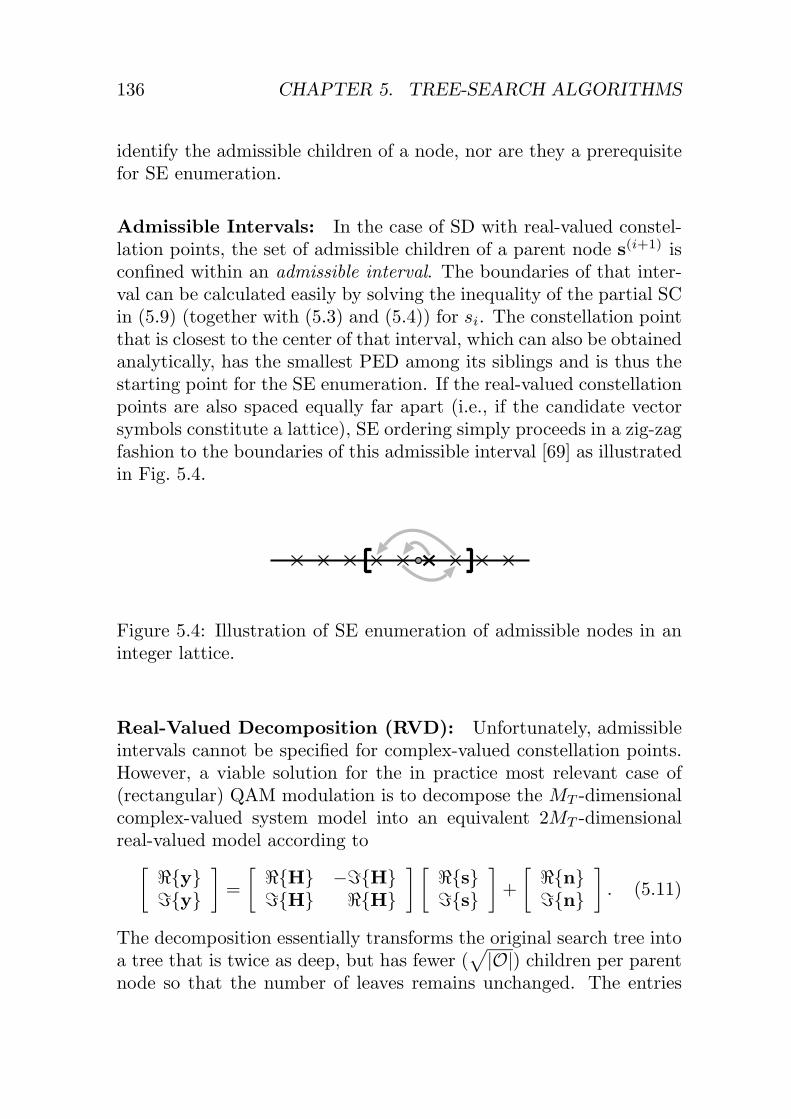
136 CHAPTER 5. TREE-SEARCH ALGORITHMS
identify the admissible children of a node, nor are they a prerequisitefor SE enumeration.
Admissible Intervals: In the case of SD with real-valued constel-lation points, the set of admissible children of a parent node s(i+1) isconfined within an admissible interval. The boundaries of that inter-val can be calculated easily by solving the inequality of the partial SCin (5.9) (together with (5.3) and (5.4)) for si. The constellation pointthat is closest to the center of that interval, which can also be obtainedanalytically, has the smallest PED among its siblings and is thus thestarting point for the SE enumeration. If the real-valued constellationpoints are also spaced equally far apart (i.e., if the candidate vectorsymbols constitute a lattice), SE ordering simply proceeds in a zig-zagfashion to the boundaries of this admissible interval [69] as illustratedin Fig. 5.4.
Figure 5.4: Illustration of SE enumeration of admissible nodes in aninteger lattice.
Real-Valued Decomposition (RVD): Unfortunately, admissibleintervals cannot be specified for complex-valued constellation points.However, a viable solution for the in practice most relevant case of(rectangular) QAM modulation is to decompose the MT -dimensionalcomplex-valued system model into an equivalent 2MT -dimensionalreal-valued model according to[
�{y}�{y}
]=
[�{H} −�{H}�{H} �{H}
] [�{s}�{s}
]+
[�{n}�{n}
]. (5.11)
The decomposition essentially transforms the original search tree intoa tree that is twice as deep, but has fewer (
√|O|) children per parent
node so that the number of leaves remains unchanged. The entries
5.1. ALGORITHM 137
of the vector symbol in (5.11) are now defined through real-valued,amplitude modulated constellation points which constitute a (finite)lattice. Hence, one can resort to computing admissible intervals and tostraightforward SE enumeration in a predefined zig-zag order accord-ing to Fig. 5.4. However, in spite of this alleged complexity advantage,it is argued later that for depth-first SD increasing the depth of thesearch tree adversely affects the performance of VLSI implementa-tions. Hence, operating directly on the complex-valued constellationsshould be preferred for SD, even if the modulation scheme permits adecomposition into an equivalent real-valued problem. As we shall seeSec. 5.3, the opposite is true for K-Best decoding.
Exhaustive-Search Enumeration
An alternative approach to exploiting a possible lattice structure foranalytically determining the admissible set of children is to explic-itly compute the PEDs of all children and to check their compliancewith the SC. The corresponding SE ordering can be obtained by sort-ing the members of the admissible set according to their associatedPEDs. The advantage of such an exhaustive approach is that one canoperate directly on arbitrary complex constellations. The drawback isthe overhead associated with the calculation of the PEDs which turnout to be dispensable because they exceed the SC and the effort forsorting the admissible children.
Direct PSK/QAM SE Enumeration
A third approach that identifies admissible intervals for depth-first SDwith complex-valued PSK or QAM constellations has been proposedby Hochwald and ten Brink in [73].
PSK-Enumeration: Based on the algorithm in [73], the SE enu-meration procedure for PSK4 constellations is introduced. The basicidea is to rewrite the SC as a function of the argument of the constella-tion points. One can then compute boundaries of admissible intervals
4With PSK, all constellation points that are arranged on a circle around theorigin.

138 CHAPTER 5. TREE-SEARCH ALGORITHMS
from the intersections of two circles, one around the origin with aradius given by the modulation scheme and one around bi+1 with aradius that corresponds to the SC.In the following, it is shown how the ideas in [73], which refer to theFinke/Pohst enumeration scheme [74], can be adapted with consider-able simplifications for the better performing SE enumeration scheme.Our modified algorithm is based on the observation that for PSK-likeconstellations∣∣∣arc(bi+1)− arc(s(l)i )
∣∣∣ < ∣∣∣arc(bi+1)− arc(s(k)i )∣∣∣ (5.12)
always implies ∣∣∣bi+1 − s(l)i Ri,i
∣∣∣ < ∣∣∣bi+1 − s(k)i Ri,i
∣∣∣ , (5.13)
where the operator arc(·) returns the phase of a complex number andwhere s
(l)i , s
(k)i ∈ O with l �= k.
The starting point for the SE enumeration s(0)i (i.e., the child that
exhibits the smallest distance increment among its siblings) can nowbe found solely based on the phases of the constellation points and ofbi+1 according to
s(0)i = arg min
si∈O|arc(bi+1)− arc(si)| . (5.14)
If the corresponding PED complies with the SC, SE enumeration cancontinue by enumerating the remaining constellation points in a zig-zag fashion as in the real-valued case, but according to their phase asillustrated in Fig. 5.5(a). The initial enumeration direction is towardsthe second-to-closest constellation point and enumeration proceedsuntil the PED associated with the current constellation point violatesthe SC [66]. Hence, explicit computation of the boundaries of theadmissible interval as is [73] is not required and it is shown later inSec. 5.2.5 how (5.14) can be evaluated in hardware without costlytrigonometric functions.
QAM-Enumeration: The direct enumeration for QAM constella-tions is a hybrid approach between direct PSK-enumeration and an
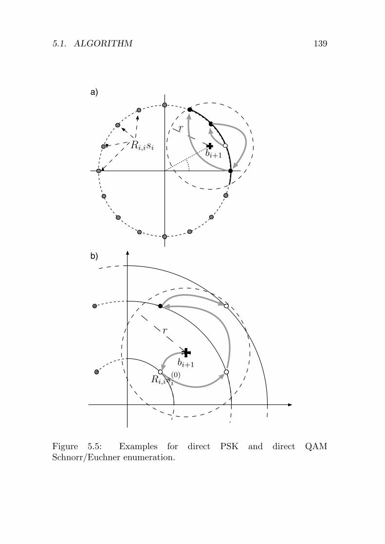
5.1. ALGORITHM 139
b)
bi+1
r
Ri,is(0)i
a)
r
bi+1
Ri,isi
Figure 5.5: Examples for direct PSK and direct QAMSchnorr/Euchner enumeration.
140 CHAPTER 5. TREE-SEARCH ALGORITHMS
exhaustive search. To this end, the QAM constellation is first de-composed into PQ subsets of PSK-like constellation points, wherebythe decomposition of QPSK, 16-QAM, and 64-QAM yields PQ =1, 3, and 9 PSK-subsets, respectively. The preferred child in each sub-set can be found according to (5.14). However, the selection of thepreferred child across subsets must be performed by explicitly compar-ing the PEDs of the PQ preferred children. Whenever a child has beenchosen the direct PSK-enumeration procedure is used to identify thenext child in that subset which then competes with the preferred chil-dren in the other subsets. When a subset contains no more admissiblechildren it is excluded from the search. An example for this enumer-ation procedure for 16-QAM modulation is shown in Fig. 5.5(b).
5.1.5 Modified Norm Algorithm
A significant portion of the silicon complexity of SD and K-Best decod-ing is in the computation of the PEDs, because the squared �2-normin (5.4) consumes considerable silicon area and because the associateddelay contributes substantially to the overall critical path. Moreover,squaring increases the dynamic range, which further increases com-plexity by aggravating numerical problems. The modified-norm algo-rithm replaces the squared �2-norm in the triangularized expression forthe PED computation in (5.2) with an approximation to the �2-normor with a different norm5. The advantages of this modification are asignificant reduction of the circuit complexity for the implementationof (5.3) and (5.4) and, as we shall see, the potential to also improvethe efficiency of the tree pruning for SD. On the negative side, opti-mum ML detection requires the use of the �2-norm. However, we shallsee that the impact of using a different norm on BER performance issmall compared to the achievable gains in terms of throughput andcircuit complexity.
The formal derivation of the modified-norm algorithm starts by takingthe square root of the PED in (5.3) and substituting xi =
√di yields
5Note that ‖y − Hs‖ = ‖y − Rs‖ only holds for the squared �2-norm. Hence,the modified-norm algorithm, described in the following, is not equivalent to theuse of a simplified norm for the original ML detection problem [75].

5.1. ALGORITHM 141
Table 5.1: Low-complexity approximations to the �2-norm accordingto f (|a| , |b|) ≈
√a2 + b2.
f (|a| , |b|)
�1-norm |a|+ |b|
�∞-norm max (|a| , |b|)
Approx.1 38 (|a|+ |b|) +
58 max (|a| , |b|)
Approx.2 max(max (|a| , |b|) , 78 max (|a| , |b|) +
12 min (|a| , |b|)
)
the following expression
xi =√
x2i+1 + |ei|2. (5.15)
The corresponding partial SC is given by xi < r which is fully equiv-alent to the original SC in (5.9). Obviously, only using the �2-norminstead of the squared �2-norm leads to an increase in circuit complex-ity due to the need for an extra squaring operation and due to theadditional costly square-root operation. In order to take advantage ofthe modified PED expression in (5.15), one can proceed to write xi
according to
xi ≈ f (|xi+1| , |ei|) , (5.16)
where f (|a| , |b|) is one of the low-complexity approximations to the�2-norm that are listed in Tbl. 5.1. What remains, when operating di-rectly on the complex-valued constellation points, is the computationof the distance increments |ei| from the real and imaginary parts ofei, which can again be computed using the approximations in Tbl. 5.1according to
|ei| ≈ f (|�{ ei }| , |� {ei}|) . (5.17)
With the RVD, (5.17) reduces to |ei| = |�{ ei }| because �{ei} = 0.We shall discuss the impact of the modified norm algorithm on theBER performance of tree-search algorithms in Sec. 5.2.3.

142 CHAPTER 5. TREE-SEARCH ALGORITHMS
5.2 Implementation of Sphere Decoding
In the following, the focus is on the VLSI implementation of the SDalgorithm. To this end, we start by introducing a suitable high-levelVLSI architecture, which is a prerequisite for the efficient implementa-tion of the depth-first tree traversal. Then, the impact of the popularreal-valued decomposition and the impact of the modified-norm al-gorithm are considered. Based on these contemplations, two RTLarchitectures and corresponding circuit-level optimizations for the SDalgorithm are presented in more detail and it is explained how theycan be pipelined. An early termination strategy is also introduced toalleviate the problem of variable throughput. Finally the section isconcluded with a summary of our implementation results.
5.2.1 High-Level VLSI Architecture
Depth-first tree traversal can be implemented efficiently with an iso-morphic one-node-per-cycle VLSI architecture in which the decodervisits a new node in each cycle and ensures that no node is ever visitedtwice. The corresponding circuit, with the high-level block diagramshown in Fig. 5.6, employs two main entities:
1. The metric computation unit (MCU) handles the forward iter-ation. To this end, the MCU receives the PED di+1 of a parentnode at its input, identifies the starting point for the SE enumer-ation, and computes the PED of the associated preferred child.If the SC is met, the decoder proceeds in forward direction tothe next level (i← i−1), choosing the preferred child as the newparent node. If the SC is violated or if the child corresponds toa leaf, the forward iteration stops and a dead-end is declared. Inthe case of a leaf, there is no need to explicitly visit the node thatcorresponds to that leaf. Instead, only the radius is updated ifd1 < r2. In conjunction with SE enumeration, this radius up-date automatically prunes all siblings of the chosen leaf fromthe tree so that none of them needs to be investigated and thedecoder can immediately start to move backwards in the tree.
2. The task of the metric enumeration unit (MEU) is to prepare

5.2. IMPLEMENTATION OF SPHERE DECODING 143
for the moment, where the forward iteration reaches a dead-endand the decoder needs to climb back up in the tree. For thatevent, the MEU constructs and maintains a list that contains onepreferred child for each node between the root and the parent ofthe node that is currently being visited by the MCU. In order toconstruct that list, which is referred to as the Preferred ChildrenCache, the MEU follows the MCU with one cycle delay andconsiders the remaining siblings of the node that is currentlybeing visited by the MCU. With SE enumeration, the siblingwith the smallest PED enters the cache. If all siblings of a nodehave already been explored or if the preferred sibling does notmeet the SC, the entry for that level remains empty. When theforward iteration stops, the MEU can immediately select a newparent node from its list (according to the depth-first paradigm)and provide the associated PED to the MCU, which can thencontinue without delay in the next cycle. Finally, the searchterminates when all entries in the list of preferred children areempty.
An example for the tree traversal procedure with the one-node-per-cycle architecture is given in Fig. 5.7. In the first three cycles, thedecoder proceeds in forward direction, feeding the output of the MCUback to its input (i.e., the preferred child of the previous cycle becomesthe parent node in the current cycle). The MEU starts with one cycledelay and chooses the nodes A’ and B’ as the preferred siblings ofnodes A and B, respectively. In cycle three, the forward iterationstops and the radius is updated by the MCU according to the PEDof the leaf C. As the MEU has already computed the PEDs of nodesA’ and B’ it can immediately determine that the PED of node B’would violate the updated SC. Thus, B’ is removed from the list ofpreferred children and node A’ is selected as the new parent node to bevisited by the MCU in the fourth cycle. Note that no time is wastedfor the backward iteration and the decoder can immediately continuein forward direction to the nodes D and finally to the leaf E. In themeantime, the MEU considers the remaining sibling of node A andthe sibling of node D for its list of preferred children. However, bothviolate the SC so that the Preferred Children Cache remains emptyand the search terminates with the final radius update at the leaf E.

144 CHAPTER 5. TREE-SEARCH ALGORITHMS
Metric Enumeration(MEU)
Metric Computation(MCU)
forwarditeration
backwarditeration
parentnode
Figure 5.6: One-node-per-cycle architecture for depth-first SD.
Computed by MCU
A A’A’’
BB’
C
D D’
E
1 24
3 2
3 5
54
Computed by MEU
Figure 5.7: Sphere Decoding example with a one-node-per-cycle VLSIarchitecture.

5.2. IMPLEMENTATION OF SPHERE DECODING 145
Complexity Metric
With the one-node-per-cycle architecture one can compute the averagethroughput of a decoder implementation according to
Φ =|O|MT
E{D}tclk, (5.18)
where tclk denotes the minimum clock cycle time and E{D} is the ex-pected number of visited nodes. The first parameter, tclk, is governedby the RTL architecture and by the circuit-level implementation, whilethe second parameter, E{D}, is determined by the efficiency of the treepruning. However, algorithm changes to reduce E{D} may affect thecritical path of the circuit and simplifications on the circuit level toreduce tclk can have a negative impact on the efficiency of the treepruning. Hence, algorithm and circuit-level optimizations must beperformed jointly in order to maximize throughput. This is consid-ered in the following.
5.2.2 Impact of the Real-Valued Decomposition
Considering the tradeoffs between the number of visited nodes and thecircuit complexity in a one-node-per-cycle architecture, the commonlyused RVD in (5.11) must be reconsidered. The main problem with theapproach for the implementation of depth-first SD is that it doublesthe depth of the search tree when compared to an algorithm thatoperates directly on the complex valued constellations. As a result,also the number of visited nodes nearly doubles [11], as illustrated inFig. 5.8 for MT = MR = 2, . . . , 7. Compensating for this loss witha reduced cycle time would require to cut the critical path into halfcompared to the critical path of an architecture that operates directlyon the complex-valued constellations. However, a comparison of thealgorithms that are available for the real-valued case to the schemesthat we use to operate directly on the complex-valued constellationsshows that only marginal gains in terms of timing can be achieved.Hence, it can be concluded that for depth-first SD operating directlyon complex-valued constellations should be preferred.

146 CHAPTER 5. TREE-SEARCH ALGORITHMS
Figure 5.8: Comparison of the number of visited nodes for SD with16-QAM constellation, with and without real-valued decomposition.
5.2.3 Impact of the Modified Norm Algorithm
The modified norm algorithm has been introduced in Sec. 5.1.5 asa means to reduce the circuit complexity of the PED computation.However, so far neither the complexity savings, nor the impact onBER performance have been quantified.
Impact on Circuit Complexity
The impact of the modified-norm algorithm on the area and the delayof the circuit that computes the PEDs is considered first. The corre-sponding schematic is shown in the top-left corner of Fig. 5.9. Theanalyzed circuit performs the norm computations according to (5.16)and (5.17), followed by a comparison which is needed to check theSC or to compare the PED to the PEDs of other nodes. The com-parator is included in the evaluation in order to better capture theimpact of the different delay profiles at the outputs of the various

5.2. IMPLEMENTATION OF SPHERE DECODING 147
norm approximation circuits. For the analysis, we always apply thesame approximation to (5.16) and (5.17). The reference circuit com-putes the squared �2-norm of a complex number in the first stage andonly performs a simple addition in the second stage, according to (5.4)and (5.3). The corresponding area/delay tradeoff curves in Fig. 5.9were obtained from automatic logic synthesis with different timingconstraints.It is interesting to see that the original squared �2-norm implemen-tation performs better in terms of silicon area and delay than theimplementations based on Approx. 1 and Approx. 2 in Tbl. 5.1. Onthe other hand, the implementations that are based on the �1- and onthe �∞-norm exhibit a much shorter critical path at lower area whencompared to the reference circuit. Compared to each other, both low-complexity implementations cover almost the same area/delay trade-off region. However, the �1-norm achieves a slightly shorter minimumcritical path and, when optimized for area-only, it provides a marginalarea advantage over an �∞-norm circuit with the same delay.
Impact on Tree-Pruning Efficiency
The use of approximations for the �2-norm alters the original SC.Hence, assessing the impact on the average decoding complexity (i.e.,the average throughput according to (5.18)) also requires an evalu-ation of the impact on the number of visited nodes. Correspondingsimulation results for a 4×4 system with 16-QAM modulation areshown in Fig. 5.10.It is interesting to see that the choice of the approximation has a con-siderable impact on the number of visited nodes. While the use ofthe �1-norm and Approx. 1 lead to a higher number of visited nodescompared to the squared �2-norm reference algorithm, complexity de-creases significantly for the �∞-norm algorithm. Only Approx. 2 hasalmost no impact on tree-pruning efficiency. At this point, it can beconcluded that Approx. 1 and Approx. 2 are not very attractive asthey neither provide an advantage in terms of silicon complexity norin terms of the number of visited nodes. Hence, we shall focus on the�1- and the �∞-norm approximations in the following.In the following, an attempt is made to give an intuitive explana-

148 CHAPTER 5. TREE-SEARCH ALGORITHMS
Figure 5.9: Area/delay tradeoff regions for computing PEDs using thesquared �2-norm and approximations to the �2-norm.
tion for the radically different number of visited nodes of the �1-, the�2- and the �∞-norm decoders. To this end, it is first noted thatfor an N -dimensional vector n with i.i.d. entries E{‖n‖1} ∝ N ,E{‖n‖2} ∝
√N , and E{‖n‖∞} ∝ logN . We now assume that the
decoder has just found the leaf that corresponds to the ML solutionsML. Unfortunately, it is not aware of this fact until the remains of thetree have been pruned completely. The average efficiency of this finaltree-pruning process is governed by the ratio between the expectedresidual radius E{d(x)1 }, where x ∈ {1, 2,∞} denotes the computationof the PED with the �1-, �2-, or �∞-norm, and the expectation for thePEDs E{d(x)i } of the remaining nodes at the higher levels of the tree(i > 1). If that ratio is small, tree pruning is likely to occur alreadyclose to the root which quickly reduces the number of visited nodes.However, if the expected residual radius is comparable or much largerthan the expected PEDs at the higher levels of the tree, the decoderis more likely to proceed to the lower levels of the tree before more

5.2. IMPLEMENTATION OF SPHERE DECODING 149
Figure 5.10: Simulation results comparing the number of visited nodeswith different �2-norm approximations to the number of visited nodeswith the original squared �2-norm SD for a 4×4 system with 16-QAMmodulation.
nodes can be pruned. By noting that d(x)1 (sML) is the norm of the
MT -dimensional error vector y − RsML, while E{d(x)i } results fromthe norm of an i-dimensional vector, it becomes intuitively clear thatthe scaling behavior of the norm with the dimension of the vector hasan impact on the ratio between these two values and thus also on thecomplexity of the depth-first SD algorithm.
Impact on BER Performance
The modified-norm tree-search algorithms no longer correspond to theML detection rule in (5.1), which immediately implies a loss in BERperformance. To quantify this loss for depth-first SD, consider thesimulation results in Fig. 5.11. Interestingly, the modified-norm algo-rithms preserve the full diversity order of the ML detector and exhibit

150 CHAPTER 5. TREE-SEARCH ALGORITHMS
no error floor. Compared to the �2-norm detector, the �1-norm algo-rithm shows a 0.4 dB SNR penalty at high SNR. The correspondingSNR penalty of the �∞-norm algorithm is slightly higher with 1.4 dB.Furthermore, simulation results for Approx. 1 and Approx. 2, whichare not shown in the chart, indicate that both approximations exhibitalmost no degradation in terms of BER performance [11].
Figure 5.11: BER performance of the �1- and the �∞-norm SD, com-pared to the BER performance of the squared �2-norm SD (250’000channel realizations).
An intuitive indication for this favorable BER behavior can alreadybe obtained from the graph in Fig. 5.12. For each level of the treethat is searched by the SD, the plot shows the ratio between the num-ber of visited nodes with the �2- and with the �∞-norm detector fordifferent SNRs. Clearly, most of the complexity reduction of the �∞-

5.2. IMPLEMENTATION OF SPHERE DECODING 151
norm algorithm happens on levels i = 2, . . . ,MT , where the �2-normdecoder visits a significantly larger number of nodes. However, thenumber of leaves that meet the SC is almost unaltered by the useof the �∞-norm. This means that both algorithms at least consideralmost the same number of candidate vector symbols in their search.Thus, one can conclude that most of the leaves that are now beingpruned earlier would have also been pruned in the original algorithm,however, at a lower level of the tree and thus less efficiently. Never-theless, it is important to note that the visited leaves for the differentnorms are not necessarily the same and that it is still possible for themodified-norm algorithm to accidentally excludes the true ML solu-tion from the search, which leads to the observed BER performancedegradation.
(Leaf) Tree level
Figure 5.12: Ratio between the number of visited nodes in the �2-normdecoder and in the �∞-norm decoder on each level of the tree for a4×4 system with 16-QAM modulation.

152 CHAPTER 5. TREE-SEARCH ALGORITHMS
Summary
The choice of a “norm”6 other than the squared �2-norm can have aconsiderable impact on complexity (on the algorithm and circuit level)and on BER performance of depth-first SD. The proposed Approx. 1and Approx. 2 ultimately increase silicon area and delay and do notreduce the number of visited nodes. Hence, they are of no furtherinterest. Approximating the squared �2-norm by the �1-norm leads toa considerable complexity reduction on the circuit level, but the sig-nificantly higher number of visited nodes outweighs the shorter criti-cal path so that with depth-first SD throughput is reduced. Finally,the �∞-norm achieves both, a reduction of the critical path (whichis almost on par with the critical path reduction associated with the�1-norm) and a reduction of the number of visited nodes. The result isa considerable gain in terms of throughput. However, this gain comesat the cost of a constant 1.4 dB high-SNR penalty in a 4×4 systemwith 16-QAM modulation.
5.2.4 SD with Exhaustive Search Enumeration
Our first implementation example for depth-first SD relies on theZF/MMSE-based preprocessing7 where the distance increments forthe PEDs are computed according to (5.7). To operate directly onthe complex-valued constellation points, the design employs the ex-haustive search enumeration method. The block diagram of the corre-sponding one-node-per-cycle VLSI architecture is shown in Fig. 5.13and is explained in detail in the following.
MCU: Sphere ALU
The silicon complexity of the MCU is governed by the repeated evalua-tion of (5.7) in the Sphere ALU for all possible incarnations of si ∈ O.
6Note that strictly speaking Approx. 1 and Approx. 2 are no norms in themathematical sense.
7Simulation results and throughput figures are based on ZF preprocessing.However it is noted that the use of MMSE preprocessing can yield higher through-puts [67] with the same hardware.

5.2. IMPLEMENTATION OF SPHERE DECODING 153
Critical Path
Sphere ALU
PED cache
MIN-SEARCH
MIN-SEARCH/ZF Select
MUX
Depth-first
MCU
MEU
Preferred children cache
forward/backwardrecursion
words(MT − 1)|O|
words(MT − 1)|O|
Figure 5.13: VLSI architecture of a depth-first SD ASIC with SEexhaustive search enumeration.
Before describing two methods for reducing this considerable complex-ity, we start by noting that the term bi+1 in (5.7) is common to allchildren of a node so that it must be computed only once. Moreover,the terms in bi+1 that depend only on R and s can be computed in apreprocessing stage in order to avoid repeated redundant calculations.In the following, the efficient VLSI implementation of the remainingparts of (5.7) is considered.
Squared �2-Norm Implementation: The first approach to effi-ciently compute the distance increments |ei|2 is based on the original

154 CHAPTER 5. TREE-SEARCH ALGORITHMS
squared �2-norm SD algorithm, which does not compromise BER per-formance. As already noted, the majority of the associated complexityis in the computation of the squared �2-norm in (5.7) which can beexpanded to
|Ri,isi − bi+1|2 = |Ri,i|2 |si|2 − 2�{(Ri,ibi+1) s∗i }+ |bi+1|2 . (5.19)
Similar to the exhaustive search ML detector described in Chap. 4,this trivial decomposition is the key to achieve further complexityreduction. The basic idea is that in (5.19) the only costly opera-tions in terms of silicon area are the evaluation of |Ri,i|2, Ri,ibi+1
and |bi+1|2. However, these terms are independent of si so that thecorresponding results must be computed only once per parent nodeand |Ri,i|2 can even be precomputed. All the remaining operationsare only multiplications of complex-valued numbers with constellationpoints (which can be realized with few adders and multiplexers [33,34, 35]) or with other constants and simple additions/subtractions.Both have a very low silicon complexity. Moreover, for the interest-ing case of QAM modulation, the real- and imaginary parts of theconstellation points si are chosen from an even smaller set of real-valued constants, which are symmetric around zero (e.g., 16-QAM:�{si},�{si} ∈ {−3,−1, 1, 3}). This property reveals further oppor-tunities for sharing intermediate results to greatly reduce the effectivenumber of computations. For a block diagram refer to [10].
�∞-Norm Implementation: Alternatively, the modified-norm al-gorithm can be employed to reduce the silicon complexity of the PEDcomputation. The corresponding part of the block diagram of a SphereALU for 16-QAM modulation is shown in Fig. 5.14 without the arith-metic units that compute bi+1. As noted previously, the absolute val-ues of the real- and imaginary parts of the |O| possible incarnations ofRi,isi are given by a small set of partial products, which can be pre-computed. For example for 16-QAM modulation, the absolute valuesof the real- and imaginary parts of Ri,isi can assume only one of twopossible values: Ri,i and 3Ri,i. Ri,i is immediately available and 3Ri,i
can be computed using a single constant-coefficient multiplier, whichis also only one adder. Appropriately adding and subtracting thesepartial products with bi+1 then yields the real and imaginary parts

5.2. IMPLEMENTATION OF SPHERE DECODING 155
f(|x|,|y|)
f(|x|,|y|)
f(|x|,|y|)
f(|x|,|y|)
f(|x|,|y|)
f(|x|,|y|)
f(|x|,|y|)
f(|x|,|y|)
f(|x|,|y|)
f(|x|,|y|)
f(|x|,|y|)
f(|x|,|y|)
SUM SUM SUMSUMSUMSUM
+1+i -1+i -1-i -3+3i -3-3i +3-3i
Ri,ixi+1bi+1
3
Ri,isi
Figure 5.14: ALU of the modified-norm exhaustive search SD.
of all ei. Computing the corresponding PEDs by using the standardsquared �2-norm algorithm (without the optimization in (5.19)) wouldrequire 2|O| squaring operations to compute the associated squared�2-norms. The result would be a prohibitive silicon complexity. Com-plexity is reduced with the �∞-norm algorithm, where each instantia-tion of a paired norm computation circuit computes the correspondingPED according to (5.16) and (5.17) with significantly lower silicon areaand delay. Nevertheless, the drawback of the modified-norm architec-ture is the large number of instantiations of 2|O| norm approximationcircuits, which becomes especially problematic for higher-order mod-ulation schemes. Unfortunately, an optimization similar to the onein (5.19) is not possible with the modified norm-algorithm. Hence,in summary, the optimized �2-norm algorithm yields an overall areaadvantage for an exhaustive search architecture.
MCU: MIN-SEARCH/ZF-Select
Once the PEDs of all children have been computed, identifying thestarting point for the SE enumeration corresponds to finding the min-imum among the |O| PEDs at the output of the Sphere ALU. The

156 CHAPTER 5. TREE-SEARCH ALGORITHMS
VLSI implementation of this MIN-SEARCH operation either relieson a prohibitively large number of parallel comparators or on a treestructure with log2 |O| levels of slow compare/select logic which isstill costly in terms of silicon area when optimized for timing. Un-fortunately, as illustrated in Fig. 5.13, the MIN-SEARCH lies on thecritical path of the circuit and due to the recursive nature of the al-gorithm, pipelining is not immediately possible.
A viable solution to this problem is to deviate from the strict SE enu-meration procedure and to make the decision on the first child to bevisited independently of the output of the Sphere ALU [9]. In thiscase, the costly MIN-SEARCH operation reduces to a simple multi-plexer which is small and fast. The challenge is to ensure that the apriori chosen child is still likely to lead to a leaf that is close to theML solution, so that the rapid shrinkage of the radius with strict SEenumeration is at least approximately maintained. Obviously, makinga random choice for the first node to be visited can not satisfy thisrequirement. However, choosing the child that corresponds to the ap-propriate entry of the sliced ZF solution s (ZF Select) yields excellentresults and is extremely simple. The strict SE ordering is resumedfor the remaining children of a node, where the SE enumeration isperformed by the MIN-SEARCH in the MEU. Simulations show thatthe loss in tree-pruning efficiency only gives rise to an approximately10% higher number of visited nodes for low and medium SNR, whilethe complexity increase becomes almost negligible at high SNR.
However, the simplified algorithm has further implications on the de-coding procedure and on complexity: Whenever a leaf is reached, thedecoder must choose the child which exhibits the smallest PED toavoid visiting the leaves. In order to meet this requirement, the mod-ified architecture compromises the one-node-per-cycle paradigm bypausing one cycle to await the result from the MIN-SEARCH in theMEU8. The same penalty applies, when the a priori chosen child doesnot meet the SC and the decoder effectively visits a node that hasalready been pruned from the tree. The corresponding performancepenalty is low (<10%) at low to medium SNRs since it is unlikelythat the node chosen by the ZF solution does not meet the SC and
8Note that for the ZF Select architecture the size of the PED cache in the MEUmust be increased from MT − 1 to MT cache lines.

5.2. IMPLEMENTATION OF SPHERE DECODING 157
because only very few visited nodes are leaves. At high SNR, theperformance degradation is more severe as the decoder often finishesin a single pass so that the average number of visited nodes increasesfrom slightly more than MT to more than MT + 1. However, on thecircuit-level the modification leads to a more than 20% reduction inthe critical path for 16-QAM modulation. Hence, at low and mediumSNR, one can leverage an overall throughput advantage. Moreover,area is slightly reduced, and the performance gain is expected to in-crease for higher order modulation schemes, where the area and thedelay of the MIN-SEARCH become even more critical.
Metric Enumeration Unit
The MEU constructs and maintains a list of preferred children in thePreferred Children Cache from which the next node to be visited isobtained using the depth-first paradigm, once the forward pass reachesa dead-end.
Construction and Maintanance of the Preferred ChildrenCache: The list of preferred children is constructed according tothe SE enumeration scheme which is realized here with an exhaus-tive search. However, an exhaustive search implementation requiresknowledge of the PEDs of all siblings of the nodes visited by theMCU on its path between the root and the current node. As the cor-responding PEDs have already been computed by the Sphere ALU inthe MCU the results can simply be kept in a PED Cache, which isMT −1 lines deep and |O| words wide and provides additional flags tomark the nodes that have already been visited. The MIN-SEARCHin the MCU now constantly considers the not yet visited siblings ofthe node that is currently visited by the MCU and the sibling with thesmallest PED is chosen to enter the corresponding line of the PreferredChildren Cache.
5.2.5 SD with PSK Enumeration
Our second implementation example of depth-first SD uses the moreefficient QR-decomposition based preprocessing and employs a low-
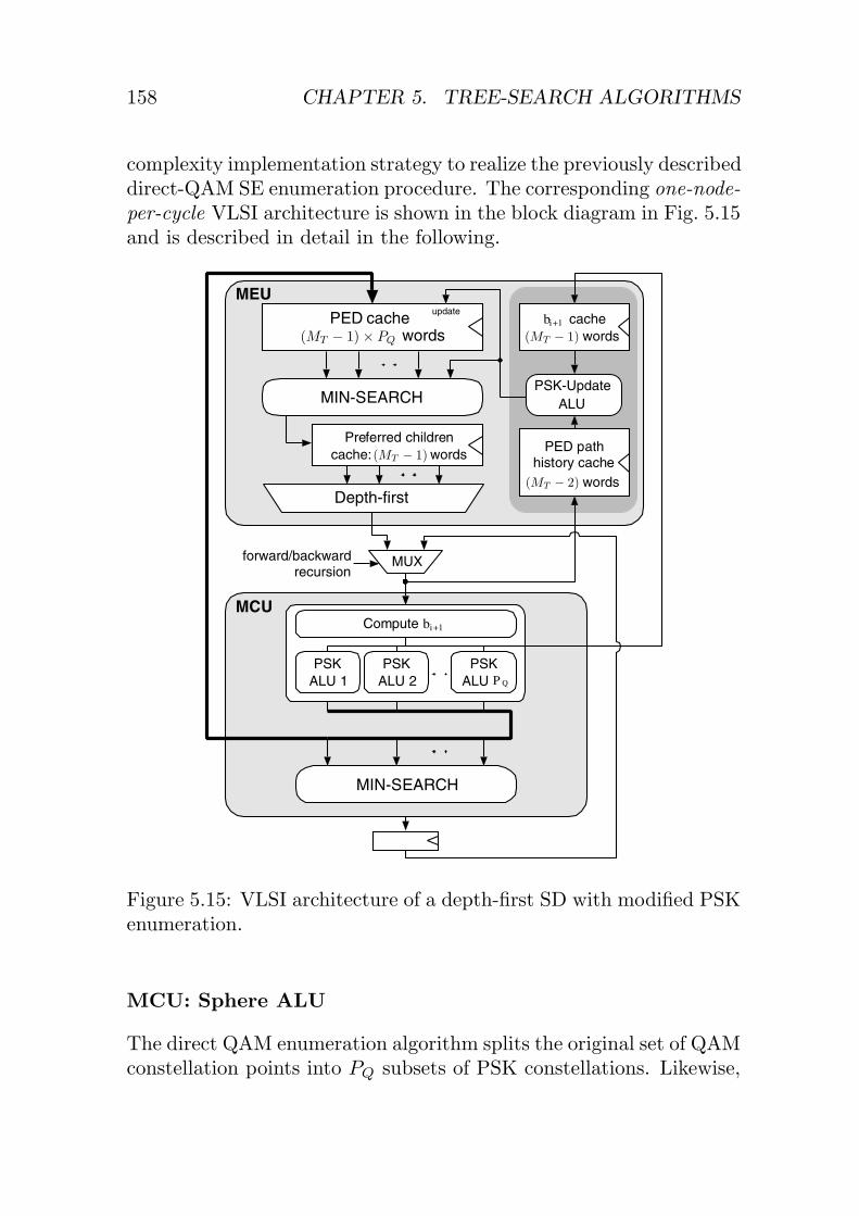
158 CHAPTER 5. TREE-SEARCH ALGORITHMS
complexity implementation strategy to realize the previously describeddirect-QAM SE enumeration procedure. The corresponding one-node-per-cycle VLSI architecture is shown in the block diagram in Fig. 5.15and is described in detail in the following.
MCU
MEU
MIN-SEARCH
Preferred children cache: words
PED cache words
PED pathhistory cache
words
cachewords
MIN-SEARCH
PSKALU 1
PSKALU 2
PSKALU
Compute
updatebi+1
bi+1
MUXforward/backwardrecursion
Depth-first
P Q
(MT − 1) × PQ (MT − 1)
(MT − 2)
(MT − 1)
ALU PSK-Update
Figure 5.15: VLSI architecture of a depth-first SD with modified PSKenumeration.
MCU: Sphere ALU
The direct QAM enumeration algorithm splits the original set of QAMconstellation points into PQ subsets of PSK constellations. Likewise,
5.2. IMPLEMENTATION OF SPHERE DECODING 159
after the computation of bi+1, the Sphere ALU employs PQ PSK-ALUs to first identify the respective starting points for the SE enu-meration (and the associated PEDs) in each of these PSK subsets.As opposed to the exhaustive search approach taken in the first SDimplementation, each PSK-ALU now only computes the PED of thepreferred child in its associated subset.
PSK-Enumeration: Finding the starting points and the initial di-rections for the SE enumeration in each PSK subset without priorknowledge of the PEDs corresponds to solving (5.14) for the closestand for the second-to-closest constellation point. The straightforwardanalytical solution is to compute arc bi+1 and to search for the constel-lation points with the smallest angular difference. This search for theclosest point can be performed by introducing and checking decisionboundaries of the form
arg minsi∈Op
|arc bi+1 − arc si| = {Op}k
if αpk < arc bi+1 ≤ αp
k+1, (5.20)
where Op contains the constellation points of the p-th PSK-subsetand where {Op}k is the k-th constellation point which is enclosed inangle space by αp
k and αpk+1. While checking the decision boundaries
is a rather simple operation for reasonably large |Op|, the approachstill suffers significantly from the prohibitive silicon complexity forcomputing arc bi+1.In the following, we shall thus develop a much more efficient solutionfor VLSI implementations. To this end, it is noted that QAM and PSKconstellations are symmetric with respect to the real and imaginaryaxes. Hence, the problem of identifying the constellation points thatare closest to bi+1 can be partially solved in the first quadrant byconsidering only bi+1, which is defined by the absolute values of thereal and imaginary parts of bi+1 according to
bi+1 = |� {bi+1}|+ j |� {bi+1}| . (5.21)
The second idea exploits the fact that the inequalities in (5.20) are in-variant under the application of a monotonically increasing function.
160 CHAPTER 5. TREE-SEARCH ALGORITHMS
Hence, in the first quadrant, we can obtain a fully equivalent expres-sion to (5.20) by considering the tangent of the decision boundarieswhich yields
αpk < arc bi+1 →
sinαpk
cosαpk
<�{bi+1}�{bi+1}
and
arc bi+1 ≤ αpk+1 →
�{bi+1}�{bi+1}
≤sinαp
k+1
cosαpk+1
. (5.22)
Noting that for QAM constellations (sinαpk/ cosα
pk) is a rational num-
ber (i.e., a number that can be expressed as a fraction of integers),one can expand the corresponding fractions in (5.22) by their denom-inators. The result are division-free inequalities which are easy tocheck in hardware as they only involve multiplications with the realand imaginary parts of constellation points (which are convenient con-stants) and a comparison. However, more importantly, as a result ofthe transformation back into Cartesian coordinates in (5.22) costlytrigonometric functions for the computation of arc bi+1 are no longerrequired and complexity is considerably reduced. Fig. 5.16(a) showsthe decision boundaries in the first quadrant for 16-QAM modulation.The associated conditions and their relevant binary relations that yieldthe starting points and the initial directions for the SE enumerationin the three PSK-subsets are listed in Fig. 5.16(b).When extending the scheme to 64-QAM modulation, the number ofrequired inequalities (i.e., decision boundaries) increases from three to15. All of them are of the form
X�{bi+1} ≷ Y �{bi+1} with X,Y ∈ {1, . . . , 7} (5.23)
which leads to a still low silicon complexity and to a low delay.Having determined the starting points and the initial enumerationdirections in each PSK-subset based on bi+1, it is finally straightfor-ward to use the sign of the real and imaginary parts of bi+1 to undothe effect of the mapping to the first quadrant with negligible circuitcomplexity.
PED Computation: Once the decisions on the starting points forthe SE enumeration in the PQ PSK-subsets have been made, the corre-

5.2. IMPLEMENTATION OF SPHERE DECODING 161
x>yx<y
2x>y2x<y
2y>x
2y<x
x>y
x<y
x>yx<y
I = �{bi+1} > �{bi+1}II = 2�{bi+1} > �{bi+1}III = �{bi+1} > 2�{bi+1}
PSK-SubsetO1 O2 O3
1 + j always 3 + j if I 3 + 3j always- 1 + 3j if I -
first step clockwiseI (I and III) or I
(I and III)
bi+1
�{bi+1}
�{bi+1}
x
ya)
b)
Figure 5.16: Low-complexity decision boundaries for finding the start-ing point for the SE enumeration and the initial enumeration directionwith 16-QAM modulation.
162 CHAPTER 5. TREE-SEARCH ALGORITHMS
sponding ALUs can proceed to compute only the associated PEDs. Tothis end, either the original �2-norm algorithm or one of the modified-norm algorithms, preferably based on the �∞-norm, may be used.
�2-norm algorithm: As opposed to the SD architecture with exhaus-tive search enumeration, the Sphere-ALU of the direct-QAM enumer-ation based decoder only needs to compute the PEDs of PQ � |O|selected children (i.e., one for each PSK subset). Due to this lowamount of parallel processing, it is not worthwhile to pursue resourcesharing according to the decomposition in (5.19). Instead, each PSK-ALU independently computes the PED of its own preferred child andonly the computation of bi+1 is shared.
�∞-norm algorithm: When fewer PEDs need to be computed in paral-lel, the positive impact on silicon complexity of the �∞-norm approx-imation becomes more pronounced. The reasons for this behavior arethe complementary effects of the less efficient resource sharing for thesquared �2-norm algorithm and the need for fewer (only 2PQ) paral-lel instantiations of the �2-norm approximation circuits which are notamenable to resource sharing. For example, for 16-QAM (64-QAM)modulation the Sphere ALU of a modified norm exhaustive searchdecoder requires 2 × 16 (2 × 64) instantiations of the correspondingnorm computation circuit, while the Sphere ALU in a direct-QAMenumeration architecture only employs 2× 3 (2× 9) instances.
MCU: MIN-SEARCH
The last step of the direct-QAM enumeration that is performed bythe MCU is to select the child with the smallest PED among therespective preferred children in the PQ PSK-subsets. Compared to theexhaustive search enumeration architecture, the corresponding MIN-SEARCH has only PQ instead of |O| inputs and is thus considerablyfaster and consumes less silicon area. For 16-QAM, for example, evena fast, fully parallel implementation merely requires the negligibleamount of four comparators. Hence, there is no reason to deviatefrom the strict SE enumeration scheme, as in the case of the exhaustivesearch enumeration based SD.

5.2. IMPLEMENTATION OF SPHERE DECODING 163
Metric Enumeration Unit
The basic structure of the MEU for direct-QAM enumeration is sim-ilar to the MEU in the exhaustive search SD architecture. The unitconstructs and maintains a list of preferred children (one for each levelbetween the root and the node that is currently visited by the MCU)according to the SE ordering. The nodes and the associated PEDsare kept in the Preferred Children Cache. Once the forward iterationreaches a dead-end, a new parent node is chosen from this cache ac-cording to the depth-first paradigm and is provided to the MCU. Thearchitectural difference to the exhaustive search enumeration basedSD lies in the method and the corresponding hardware that is usedfor the construction and maintanance of this list of preferred children.
Construction and Maintenance of the Preferred ChildrenCache: While the MCU visits a parent node on level i+1, the MEUmust choose one of the remaining siblings of that node, according tothe SE enumeration procedure, to enter the Preferred Children Cache.With direct QAM enumeration, this choice only requires knowledgeof the PEDs of the corresponding preferred children in the PQ PSK-subsets. To this end, each line in the PED Cache keeps these childrenand the associated PEDs. As opposed to the exhaustive search SDarchitecture which requires |O| entries per cache line, the PED cachein the direct QAM architecture requires only PQ � |O| entries percache line. The first set of children to enter a line in the PED Cacheis identified by the MCU in the forward pass. However, one of themhas also already been chosen as the next parent node so that only theremaining PQ − 1 candidates can immediately enter the PED Cache.The consumed child must be replaced by the next constellation pointin the corresponding PSK-subset, according to the direct PSK enu-meration scheme, before a preferred child can be selected from thatcache line to enter the Preferred Children Cache. Similarly, whenthe MCU consumes an entry from the Preferred Children Cache in abackward iteration, the corresponding entry in the PED Cache mustbe updated before a new node can be identified to replace the cho-sen node in the Preferred Children Cache. Only if all constellationpoints in a PSK-subset have been considered, the corresponding en-try in the cache line is marked as invalid and is ignored by the unit

164 CHAPTER 5. TREE-SEARCH ALGORITHMS
that maintains the Preferred Children Cache.
Updating consumed entries in the PED Cache follows the predefinedorder of the direct PSK-enumeration scheme. Hence, no checking ofdecision boundaries is required and the PED of the next constellationpoint must only be computed in the PSK-Update ALU. Most of thecomplexity of this operation is in the computation of the term bi+1
in (5.4). However, this term is common to all siblings that are con-sidered by the MEU and has already been computed by the MCU.Thus, it can be kept in a small bi+1 Cache in the MEU in order toavoid replicating the costly hardware for its computation. Finally, thecomputation of PEDs on level i+1 requires knowledge of the PED oftheir parent node on level i+ 2. Therefore, an additional small PEDPath History Cache with MT − 2 entries is required, which stores thePEDs of the nodes on the path between the root and the current node.
Remarks:
As a final remark, we shall mention here that, strictly speaking, thecombination of the �∞-norm algorithm with direct QAM enumera-tion yields an algorithm which is neither �2 nor �∞. The reason forthis is the fact that the phase-based PSK enumeration within a PSK-subset imposes an ordering that corresponds to the �2-norm, whilethe choice across subsets is based on PEDs that have been computedusing the �∞-norm. As a result, the solution found by the decoderand the exact number of visited nodes may deviate slightly from anexhaustive search enumeration based implementation of the �∞-normSD algorithm. However, simulations have shown that the differenceis extremely small and yields not visible difference in the BER perfor-mance or in the number of visited nodes.
5.2.6 Pipelined Depth-First Sphere Decoder
Pipelining of a one-node-per-cycle architecture is not immediately pos-sible due to the recursive nature of the depth-first SD algorithm. Nev-ertheless, a simple, well known trick [57] can be used to circumventthis bottleneck.

5.2. IMPLEMENTATION OF SPHERE DECODING 165
The basic idea is extremely simple and exploits the fact that the decod-ing of multiple subsequent vector symbols in a MIMO communicationsystem is performed independently of each other. On the architec-tural level, one can thus simply introduce K − 1 additional pipelineregisters into the original, unpipelined decoder to obtain K pipelinestages. Due to the recursive nature of the depth-first SD algorithm,pipeline bubbles must be introduced to ensure that the original al-gorithm is not altered. Unfortunately, these pipeline bubbles nullifythe performance gains that are achieved from the higher admissibleclock rates after pipelining. However, if multiple symbols need to bedecoded, the pipeline bubbles can be filled with other received vectorsso that the decoder effectively processes multiple symbols in parallelin an interleaved fashion. Hence, as a result of the K-fold pipelining,the throughput can be increased up to K-fold. However, in practice,this gain will be lower, due to the nonideal placement of the pipelineregisters in the critical path and due to the increasing share of setupand hold on the overall timing budget. On the other hand, pipeliningonly increases the amount of registers in the design, so that also thearea is expected to grow less than proportional to K. Hence, an over-all efficiency advantage is obtained for a reasonable number of pipelinestages (2–4).
5.2.7 Sphere Decoding With Early Termination
The main problem with the application of depth-first SD in practicalsystems is the variable instantaneous throughput which – only on av-erage (over different symbols, channels, and noise realizations) – is afunction of the SNR. In a one-node-per-cycle architecture, the worst-case decoding delay for a symbol corresponds to the number of clockcycles that is required to visit all nodes in the tree (excluding theleaves) which is given by
Dmax =|O|MT
|O| − 1 . (5.24)
Unfortunately, Dmax exceeds by far the average complexity E{D}based on which an efficient decoder must be designed. Hence, re-ceived vectors requiring a decoding effort far above the capabilities

166 CHAPTER 5. TREE-SEARCH ALGORITHMS
of the implementation cause latencies in the decoding process whichmust be absorbed with potentially large FIFO memories or whichmay not even be tolerated due to tight latency constraints imposedby higher-layer protocols.
Early Termination without Coding
An obvious solution to the problem of variable decoding time is tosimply constrain the search time (i.e., the number of visited nodes).Once the decoder exceeds this limit, it stops and returns the bestsolution it has found so far. Clearly, such an approach will degrade theBER performance as illustrated by the simulations results in Fig. 5.17.
A large number of optimizations can be employed to reduce the per-formance loss shown in Fig. 5.17. Such methods include for exampleoptimizing the detection order [66, 70, 71], MMSE preprocessing [67]or the use of FIFOs and block processing [72], which allows to con-strain the aggregate decoding effort over a number of received vectors.However, none of these techniques can fully close the significant per-formance gap that is visible in Fig. 5.17.
A Solution to Early Termination With BICM
In order to develop an algorithm that mitigates the BER performanceloss of depth-first SDs with early termination we must extend ourview to also take the capabilities channel coding into account. In thefollowing, the most relevant case of bit interleaved coded modulation(BICM) [14] is assumed.
MIMO-BICM System Model: In the system under considera-tion, the data is first encoded with a convolutional encoder9. Thebits at the output of the encoder are then interleaved using a randominterleaver before they are transmitted from the MT transmit anten-nas in spatial multiplexing mode. The receiver (shown in Fig. 5.18)
9For our simulations we use a rate 1/2 code with constraint length 7 whose gen-erator polynomials are defined by [133o, 171o]. Furthermore, per-antenna codingis assumed.

5.2. IMPLEMENTATION OF SPHERE DECODING 167
Figure 5.17: BER performance of �2-norm SD for a 4×4 system with16-QAM modulation. The maximum number of visited nodes wasconstrained to Dmax = 7, 10, 13, 16, 19, 22 and results are comparedto the BER performance of a corresponding SD without runtime con-straints (250’000 channel realizations).
consists of a MIMO detector and a Viterbi decoder, linked by a dein-terleaver. A regular SD provides binary (hard) decisions b
(i)m at its
MIMODetector
(Viterbi)Decoder
∏−1
yH b
(i)m
Figure 5.18: High-level architecture of a MIMO BICM receiver.
output. However, a subsequent soft-input Viterbi decoder can takeadvantage of reliability information about the received bits. To this

168 CHAPTER 5. TREE-SEARCH ALGORITHMS
end, soft-output MIMO detectors [76, 77, 7, 73, 64, 63] obtain (approx-imate) log-likelihood ratios (LLRs). Assuming no a-priori knowledgeof the transmitted data stream (P (b(i)m = 0) = P (b(i)m = 1) = 1/2),these LLRs are defined according to
L(b(i)m
)= log
(P (b(i)m = 0|y,H, σ2)
P (b(i)m = 1|y,H, σ2)
), (5.25)
where P (b(i)m = 0|y,H, σ2) and P (b(i)m = 1|y,H, σ2) denote the a-posteriori probabilities that the i-th bit in the constellation transmit-ted from the m-th antenna is 0 or 1, respectively.
In this work, the discussion has been limited to hard-decision MIMOdetectors which have a much lower complexity compared to most soft-output MIMO decoders. However, it is shown in the following how theability of a Viterbi decoder in order to process reliability informationcan be exploited to mitigate the performance degradation of SphereDecoders with early termination.
Computing Approximate LLRs for Hard-Decision MIMODe-tectors: The algorithm described in the following is based on ourlow-complexity approach to derive soft information solely based onchannel state information [78]. The fundamental idea is to computeapproximate LLRs based on a-posteriori probabilities which are con-ditioned on the output of the detector b
(i)m and on various kinds of
side information (summarized in the set T ) which allows to estimatethe reliability of these decisions. The corresponding formal equationis given by
L(b(i)m
)= log
(P (b(i)m = 0|b(i)m , T )P (b(i)m = 1|b(i)m , T )
). (5.26)
Assuming the demodulator has a symmetric error probability so that
P (b(i)m �= b(i)m |T ) = P (b(i)m �= 0|b(i)m = 0, T )= P (b(i)m �= 1|b(i)m = 1, T ), (5.27)

5.2. IMPLEMENTATION OF SPHERE DECODING 169
one can write (5.26) as
L(b(i)m ) =
{R(i)m (T ), b
(i)m = 0
−R(i)m (T ), b
(i)m = 1
with
R(i)m (T ) = log
(1− P (b(i)m �= b
(i)m |T )
P (b(i)m �= b(i)m |T )
)(5.28)
because P (b(i)m = b(i)m |T ) = 1− P (b(i)m �= b
(i)m |T ).
Application to Sphere Decoding with Early Termination: ForSD with early termination T is comprised of two important pieces ofinformation which give a clue about the reliability of the decision ofthe decoder for a particular bit:
1. The average received SNR and
2. the information whether the depth-first search for the ML so-lution was completed within the given runtime constraint orwhether it had to be be terminated prematurely.
Conditioned on both parameters, one can obtain estimates of the as-sociated average BER performance P (b(i)m �= b
(i)m |T ) of the MIMO de-
tector by means of simulations. The corresponding R(i)m (T ) can then
be obtained from (5.28) and can be stored in a two-dimensional look-up-table. During decoding, this table is indexed by the binary earlytermination indicator of the SD and by the quantized SNR value asshown in the block diagram in Fig. 5.19.
Impact on BER Performance: To study the impact of the pro-posed method on the coded BER performance, consider the simulationresults in Fig. 5.20. In the example for a 4×4 system with 16-QAMmodulation, the maximum number of visited nodes was constrained toDmax = 710 and independent channel realizations were chosen for thetransmission of subsequent vector symbols. Without soft-information,
10In a 4×4 system, Dmax = 7 corresponds to the number of visited nodes whenthe SD traverses the tree twice from the root to the leaf.

170 CHAPTER 5. TREE-SEARCH ALGORITHMS
ySphere decoder
withearly termination
H Viterbidecoder
∏−1
SNR LLR LUT
indicates earlytermination
T
b(i)m
R(i)m (T )
0/1
L(b(i)m
)
Dmin
Figure 5.19: High-level architecture of a MIMO BICM receiver withsphere decoder with early termination.
early termination leads to a loss of diversity and causes a consider-able SNR penalty (> 4 dB for BER=10−5) which increases for morestringent BER requirements. The improved receiver architecture inFig. 5.19 suffers only from a constant SNR penalty of 0.9 dB com-pared to the SD with no runtime constraints. Further evaluationsshow that an additional FIFO buffer for five received vectors is suffi-cient to improve the BER performance of the early-terminated SD towithin 0.2 dB of the unconstrained decoder.
Impact on Silicon Complexity: With respect to silicon complex-ity, only a negligible overhead is required for the generation of thesoft outputs for a hard decision SD with early termination. The rea-son for this is that the BER performance of the described algorithm ishighly insensitive to the accuracy of R(i)
m (T ) with respect to the SNR.Hence, the corresponding LUT requires only very few entries. Mostof the additional area comes from the use of a Viterbi decoder withsoft inputs. However, implementation results also show that the asso-ciated increase in the number of gates is small compared to the totalarea requirement for a high-throughput Viterbi decoder. Finally, it isnoted that in OFDM systems received vectors are anyway processedin blocks so that also the use of a runtime constraint over a block ofsymbols comes at no additional area expenditure.

5.2. IMPLEMENTATION OF SPHERE DECODING 171
3.5 dB
0.8 dB
Figure 5.20: Coded BER performance of SD (with sorted QR pre-processing) for different early termination strategies in a 4×4 systemwith 16-QAM modulation (15’000 code blocks).

172 CHAPTER 5. TREE-SEARCH ALGORITHMS
5.2.8 Implementation Results
In the following, implementation results for SD in a 4×4 system with16-QAM modulation are considered in order to compare the differ-ent architectural choices with respect to their impact on silicon area,BER performance and throughput. After that, the scaling behaviorof depth-first SD architectures towards higher rates is discussed andreference implementation results are given for a 6× 6 system with 16-QAM modulation and for a 4×4 system with 64-QAM modulation.
Comparison of Architectural Choices for SD
In order to compare the architectural choices for depth-first SD con-sider the implementation results in Tbl. 5.2. The corresponding aver-age throughput and the guaranteed minimum throughput character-istics with early termination (for Dmax = 7) for the three referencedesigns are shown in Fig. 5.21. The first design (according to Arch. I)employs an exhaustive search enumeration strategy and is based onthe squared �2-norm algorithm. The details of its RTL implementa-tion follow the description in Sec. 5.2.4. The second ASIC (accordingto Arch. II) is based on the direct-QAM enumeration strategy and usesthe �∞-norm approximation. The third ASIC is a pipelined versionof Arch. II which processes three symbols in parallel in an interleavedfashion to achieve a higher clock rate. The chip micrograph and thelayout in Fig. 5.22 correspond to the implementations of Arch. I andArch. II (ASIC-I and ASIC-II) reported in [9] and [10]11.
Arch. I vs. Arch II: As can be seen from Fig. 5.21 and Tbl. 5.2,Arch. II achieves more than twice the throughput (average and withearly termination) of Arch. I at the same SNR, while it only consumesless than half of the silicon area of the first design.The considerable throughput improvement of the second design canmostly be attributed to the reduction in the number of visited nodes
11Note that in the following we refer to our latest synthesis results for whichdetails of ASIC-II have been partially revised since the publication of [10] to im-prove timing and to reduce area. The corresponding performance estimates donot include layout parasitics to facilitate a fair comparison to the pipelined SDand to other MIMO detectors for which no layouts are available.
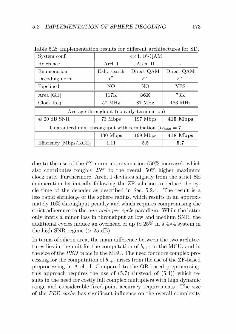
5.2. IMPLEMENTATION OF SPHERE DECODING 173
Table 5.2: Implementation results for different architectures for SD.System conf. 4×4, 16-QAMReference Arch I Arch. II -
Enumeration Exh. search Direct-QAM Direct-QAM
Decoding norm 2 ∞ ∞
Pipelined NO NO YES
Area [GE] 117K 36K 73K
Clock freq. 57 MHz 87 MHz 183 MHz
Average throughput (no early termination)
@ 20 dB SNR 73 Mbps 197 Mbps 415 Mbps
Guaranteed min. throughput with termination (Dmax = 7)
130 Mbps 199 Mbps 418 Mbps
Efficiency [Mbps/KGE] 1.11 5.5 5.7
due to the use of the �∞-norm approximation (50% increase), whichalso contributes roughly 25% to the overall 50% higher maximumclock rate. Furthermore, Arch. I deviates slightly from the strict SEenumeration by initially following the ZF-solution to reduce the cy-cle time of the decoder as described in Sec. 5.2.4. The result is aless rapid shrinkage of the sphere radius, which results in an approxi-mately 10% throughput penalty and which requires compromising thestrict adherence to the one-node-per-cycle paradigm. While the latteronly infers a minor loss in throughput at low and medium SNR, theadditional cycles induce an overhead of up to 25% in a 4×4 system inthe high-SNR regime (> 25 dB).
In terms of silicon area, the main difference between the two architec-tures lies in the unit for the computation of bi+1 in the MCU, and inthe size of the PED cache in the MEU. The need for more complex pro-cessing for the computation of bi+1 arises from the use of the ZF-basedpreprocessing in Arch. I. Compared to the QR-based preprocessing,this approach requires the use of (5.7) (instead of (5.4)) which re-sults in the need for costly full complex multipliers with high dynamicrange and considerable fixed-point accuracy requirements. The sizeof the PED-cache has significant influence on the overall complexity

174 CHAPTER 5. TREE-SEARCH ALGORITHMS
Figure 5.21: Throughput comparison of different VLSI architecturesfor the implementation of depth-first Sphere Decoding.
of the design, as parallel access requirements call for an implementa-tion based on registers and standard cells instead of RAMs. Hence,the need for a larger PED Cache in Arch. I due to the use of theexhaustive search enumeration has a significant impact on the overallsilicon area. For 16-QAM, the approach requires storage for |O| = 16PEDs in each cache line, as opposed to the direct-QAM enumerationmethod in Arch. II, where each cache line must only contain PQ = 3entries. Moreover, the deviation from the strict SE ordering in Arch. Iultimately also entails the need to increase the number of cache linesfrom MT − 1 to MT .
Finally, without early termination, Arch. I achieves full ML perfor-mance as it is based on the squared �2-norm criterion. The use of the�∞-norm approximation in Arch. II leads to a constant 1.4 dB high-SNR penalty in a 4×4 system with 16-QAM modulation. Neverthe-

5.2. IMPLEMENTATION OF SPHERE DECODING 175
less, the approximation preserves the diversity order of a ML detector.Fixed-point simulations of both reference designs have shown that upto at least 30 dB SNR, finite wordlength effects show no visible im-pact on the BER performance. However, the use of QR-preprocessingand of the �∞-norm considerably relax wordlength requirements infixed-point implementations.
Impact of Pipelining: The third reference design in Tbl. 5.2 andFig. 5.21 is a pipelined version of Arch. II. Its three pipeline stagesrequire two additional sets of registers and allow for a 2.1× increase inclock frequency and for a corresponding increase in average through-put. At the same time, the area of the design increases by almosta factor of two. Hence, the overall circuit efficiency only increasesslightly but pipelining still provides an advantage over two parallelinstantiations of the same design. The main reason for the sublinearincrease in terms of throughput lies in the difficulty to balance the de-lays of the pipeline stages and the considerable area overhead is due tothe fact that interleaved processing of symbols with different channelsrequires costly register-based storage for multiple R matrices. How-ever, it is also noted that a more carefull automated retiming of thepipeline registers has the potential for further improvements in termsof throughput and that the area overhead from additional registers ismuch less pronounced in cases where subsequent symbols share thesame channel realization.
Complexity Scaling Behavior
In the following, the scaling behavior of the presented architecturestowards higher rates is considered.
Tree Pruning: Before analyzing the impact of higher rates on thecircuit complexity and on the cycle time, the impact on the efficiencyof the tree pruning (i.e., E{D} in (5.18)) is investigated. Becauseno analytical expressions are available for the employed algorithm,we resort to the simulation results in Fig. 5.23. The chart gives thenumber of visited nodes for R = 16 (4×4 with 16-QAM) and forR = 24 bpcu (6 × 6 with 16-QAM and 4×4 with 64-QAM). For low

176 CHAPTER 5. TREE-SEARCH ALGORITHMS
Core area: 50K GE,Clock freq.: 71 MHz
Core area: 117K GE,Clock freq.: 51 MHz
Figure 5.22: Chip micrograph of the SD ASICs, reported in [9] and[10] for 4×4 systems with 16-QAM modulation, implemented in a0.25µm CMOS technology.
and medium SNRs, both R = 24 decoders exhibit a similar number ofvisited nodes which is significantly larger compared to R = 16 bpcu.In the high-SNR regime, the average number of visited nodes ap-proaches MT . Hence, in terms of the number of visited nodes thesystem that achieves the higher rate with a higher order modulationscheme has an advantage over a system that achieves the same rateby increasing the number of antennas.
Exhaustive Search Enumeration Architecture: Being awareof the implications of higher rates on the algorithm side, we shallnow consider the impact on circuit complexity for exhaustive searchbased SD architectures. The corresponding silicon area grows almostlinearly with the number of antennas, but exponentially with the orderof the modulation scheme. In both cases, the main increase in area isdue to the larger PED Cache which constitutes a significant portionof the overall circuit. However, while implementations for MT = 6are still feasible with this architecture, implementations for 64-QAMexceed the limits of an economic implementation because each line inthe PED Cache would require 64 instead of 16 (for 16-QAM) entries.In terms of timing, increasing MT has only a minor impact on the

5.2. IMPLEMENTATION OF SPHERE DECODING 177
Figure 5.23: Number of visited nodes for �∞-norm Sphere Decodingfor 16 bpcu (4×4, 16-QAM) and for 24 bpcu (6×6, 16-QAM and 4×4,64-QAM).
clock frequency of the design compared to the increase in terms of thenumber of visited nodes.
Direct-QAM Enumeration Architecture: The order of the scal-ing behavior of the direct-QAM enumeration architecture is the sameas for the exhaustive search based SD. However, for most practicalcases, the circuit complexity for a direct-QAM enumeration based SDscales more favorably with the rate, especially when increasing theorder of the modulation scheme. The main reason for this behavior isthe significantly smaller PED Cache, which requires only PQ insteadof |O| entries per cache line. For 64-QAM, for example, PQ = 9 wordsper cache line are sufficient. In terms of timing, increasing the mod-ulation scheme will have a greater impact than increasing MT . The

178 CHAPTER 5. TREE-SEARCH ALGORITHMS
reason is the fact that most of the critical path is in the MCU, whosedesign is mostly independent ofMT , but which is strongly affected byincreasing the modulation order.
Table 5.3: Silicon complexity of SDs for systems with 16 and 24 bpcu.System conf. 4×4, 16-QAM 6× 6, 16-QAM 4×4, 64-QAMRate [bpcu] 16 24 24
Optimized for timing
Area [GE] 36K 59K 66K
Clock freq. 87 MHz 79 MHz 72 MHz
Avrg. throughput 197 Mbps 105 Mbps 86 Mbps
@ 20 dB SNR
Avrg. throughput 253 Mbps 158 Mbps 173 Mbps
@ 25 dB SNR
Optimized for area
Area [GE] 22K 36K 42K
Clock freq.12 40 MHz 40 MHz 34 MHz
Reference Implementations of Arch. II for 24 bpcu: Despitethese obvious architectural implications of higher rates, reliable esti-mates of the true silicon complexity of the corresponding decoders re-quire the consideration of actual implementation results. Tbl. 5.3 pro-vides reference for area, cycle times (tclk), and throughput of SphereDecoders for 4×4 systems with 16-QAM and 64-QAM modulationand for 6 × 6 systems with 16-QAM modulation. Basic design spaceexploration is performed by optimizing the designs for timing-onlyand area-only, respectively. All presented designs still show moderatesilicon area. Notably, the reduction of the maximum clock frequencyfor the higher-rate designs is in all cases low, compared to the increasein terms of number of visited nodes at low and medium SNR. As ex-pected, the use of 64-QAM proves to be more expensive in terms ofarea and delay compared to the design that achieves R = 24 bpcuwith 16-QAM modulation and MT = 6.Simply optimizing for low area leads to designs that are roughly 28%

5.2. IMPLEMENTATION OF SPHERE DECODING 179
smaller, but also 50% slower than the corresponding performance op-timized designs. Hence, optimizing for timing yields the highest hard-ware efficiency.

180 CHAPTER 5. TREE-SEARCH ALGORITHMS
5.3 Implementation of K-Best Decoding
In this section, the VLSI implementation of a high-throughput K-Bestdecoder is considered. To this end, a suitable high-level architectureis described first. We then investigate the implications of the RVD,described in Sec. 5.1.4, on the K-Best algorithm. Finally, the RTL im-plementation is explained in more detail and reference implementationresults are presented.
5.3.1 High-Level VLSI Architecture
An efficient pipelined linear array architecture for the implementa-tion of the K-Best algorithm has originally been proposed in [24] andwas later adopted by other authors for various implementations ofthe same algorithm [79, 80, 81]. The corresponding block diagramis shown in Fig. 5.24. Essentially, the circuit is composed of a linear
Sort(Merge)MCU
L(i+1)K
KBU
L(i)K
yi
Ri
i = 1i = MT
y
R1 R2 R2MTR3
i = MT − 1
ProcessingElement
Par
ent N
ode
Cac
he
Pre
ferr
edC
hild
ren
Cac
he
Figure 5.24: High-level pipelined linear array architecture for K-BestMIMO detection.
array of processing elements (PEs), which are directly associated with

5.3. IMPLEMENTATION OF K-BEST DECODING 181
the levels of the search tree. Hence, a K-Best decoder which operatesdirectly on complex-valued constellations requires MT PEs, while anarchitecture that uses the RVD employs 2MT PEs. In each step, thei-th PE receives a list L(i+1)
K ofK admissible nodes from the precedingPE (i+1). The entries of that list contain the partial candidate vectorsymbols si+1 of the admissible nodes and the associated PEDs di+1.The task of a PE is to visit these (parent) nodes and to identify a setL(i)
K of K preferred children which are then passed on to the next PE(L(i)
K ← L(i)K ).
Processing Elements: Similar to previous implementations of K-Best decoding, we use an exhaustive search approach to identify theK preferred children in each PE. Because of the complexity that isassociated with the identification of these children of K parent nodessome degree of resource sharing [57] within the PEs will be necessaryin order to reduce the hardware complexity. Nevertheless, our imple-mentation of the PEs applies a more parallel approach compared tothe other reported implementations of the algoithm.
The architecture of a PE consists of a Parent Node Cache, a metriccomputation unit (MCU) and of a K-Best unit (KBU) with a Pre-ferred Children Cache. The Parent Node Cache which contains L(i+1)
K
represents the pipeline register between the subsequent stages of thehigh-level architecture. Its entries are read by the MCU which ob-tains the PEDs of all associated children according to (5.3) and (5.4).The results of this computation then enter the input register of theKBU, which keeps track of the K nodes with the smallest PEDs in itsPreferred Children Cache. Once all children of all admissible parentnodes have been considered, one step is complete and the output ofthe KBU can be forwarded to the next PE.
5.3.2 Impact of the Real-Valued Decomposition
Recall from Sec. 5.1.4 that for rectangular QAM constellations asearch tree can either be constructed based on the complex-valuedconstellations or using the RVD in (5.11). In order to compare thetwo algorithm choices, we shall assess the impact on the silicon area,

182 CHAPTER 5. TREE-SEARCH ALGORITHMS
the throughput and on the BER performance, under the assumptionthat the design parameter K remains fixed.
Impact on Silicon Complexity: For estimating the impact oncomplexity, first consider the high-level architecture, where using theRVD doubles the number of PEs and thus also doubles the numberof pipeline stages in the decoder. By itself, this modification mayonly give rise to a higher decoding latency, but it should not have animpact on the throughput of the circuit [57]. However, a comparisonof the two approaches to construct a search tree must also take intoaccount the impact on the complexity of the PEs. To this end, thenumber of children which must be considered by the MCU and amongwhich the associated KBU needs to choose the K preferred childrenfor the next PE is counted: It is found that, when operating directlyon the complex-valued constellation points, an MCU must computeK|O| PEDs in each step, while this number reduces significantly toonly K
√|O| PEDs when the RVD is employed. This lower number
of candidates not only affects the complexity of the MCU, but alsoreduces the complexity of the KBU since the same number of nodes(K) must be chosen from a smaller list of candidates. Moreover, inthe real-valued case, also the complexity of the PED computationis considerably reduced. Hence, we conclude that the overall siliconcomplexity of the individual PE is much lower with the RVD whichmore than compensates for the larger number of PEs (2MT insteadof MT ).
Impact on BER Performance: For the consideration of the im-pact of the RVD on the BER performance, K = 5 is used and sortedQR [70, 72] decomposition is employed for the preprocessing. Cor-responding BER simulation results for a 4×4 system with 16-QAMmodulation are shown in Fig. 5.25. Surprisingly, the graph shows aconsiderable advantage of the K-Best algorithm with RVD in termsof BER performance compared to the K-Best decoder which operatesdirectly on the complex-valued QAM constellation points.An intuitive explanation of this interesting behavior can be borrowedfrom [82] where a similar behavior has been observed when the V-BLAST SIC scheme is applied to the RVD of the input-output rela-

5.3. IMPLEMENTATION OF K-BEST DECODING 183
NoNo
Figure 5.25: BER performance comparison of K-Best decoders (K =5, sorted QR preprocessing) with and without RVD and with �2- and�1-norm (600’000 channel realizations).
tion of a MIMO system, instead of directly solving the complex-valuedproblem. In order to relate these results to K-Best decoding, it is notedthat the K-Best algorithm is similar to SIC with the exception thatmore than one hypothesis can be explored. We further recall that thebasic idea behind SIC is to improve the detection of the remainingstreams by subtracting (i.e., cancelling) the interference from alreadydetected streams and that the streams which are detected first13 thusare the most vulnerable to detection errors. However, it is also recog-nized that in the complex-valued case, where real and imaginary partsof the same stream are orthogonal, the detection of one of the twocomponents has no influence on the detection of the other component
13These streams correspond to the levels closer to the root of the search tree inK-Best decoding.

184 CHAPTER 5. TREE-SEARCH ALGORITHMS
of the same stream and can thus not improve its detection reliability.The fundamental idea that explains the BER performance improve-ment from the RVD in (5.11) is that separating the real and imaginaryparts allows to start with the detection of only one of the two compo-nents of the vulnerable first stream, while choosing a component froma different stream as the second in the detection order14. As opposedto the quadrature component of the first stream, this component ofanother stream can already profit from the interference cancellationdue to the partially detected first stream. To illustrate this effect, weuse simulations for MT = 4 to obtain the probability density function(pdf) of the power of the diagonal entries of R and R which are ob-tained from sorted QR decomposition of the complex-valued channelmatrix H and of the corresponding channel matrix after RVD, respec-tively. In Fig. 5.26 the focus is on Ri,i for i =MT − 1 and i =MT forthe complex-valued case and on Rj,j for j = 2(MT − 1)− 1, . . . , 2MT
for the real-valued case. In terms of error probability, these entriescorrespond to the four weakest quadrature components of the trans-mitted data stream. Clearly, the RVD cannot improve the detectionquality of the first quadrature component, which in a symmetric setup(MR = MT ) still suffers from a severe lack of diversity. However, inthe complex-valued case, R4,4 is also used to detect the correspondingorthogonal component of the first stream, which thus suffers equallyfrom the same lack of diversity. With the RVD, the error probabil-ity of the second quadrature component (which is not the one that isorthogonal to the component that was detected first) is governed byR7,7 which shows a considerably more robust distribution. Hence, theassociated error probability is reduced. Unfortunately, this gain canonly be leveraged for the second stream. As can also be seen fromFig. 5.26, the distribution of R6,6 which is responsible for the reliabil-ity of the detection of the third quadrature component with the RVDis slightly less robust than the distribution of R3,3, which is used torecover the third and the fourth quadrature components of the trans-mitted vector symbol in the complex-valued case. Nevertheless, asthe extremely weak first stream dominates the BER performance of aSIC decoder and of the K-Best decoder, an overall BER performance
14Note that a RVD which arranges the real and imaginary parts of the samestream in adjacent rows (as opposed to the arrangement in (5.11)) yields no per-formance improvement over the complex-valued case.

5.3. IMPLEMENTATION OF K-BEST DECODING 185
Figure 5.26: Empirical probability density function of the channelgains after sorted QR decomposition with and without RVD.
advantage is obtained from the use of the RVD.
Summary: We conclude that for the implementation of the K-Bestalgorithm the use of the RVD should be preferred over a decoder thatoperates directly on the complex-valued constellation points. Hence,we shall focus on the K-Best decoding with RVD in the following.
5.3.3 Throughput-Optimized Implementation
All K-Best decoders reported in the literature [24, 79, 80, 81] rely onconsiderable resource sharing for the implementation of the PEs. Thecorresponding architectural concept is to compute all K
√|O| children
of the admissible parent nodes sequentially in the MCU and to usea low-complexity bubble-sort unit to generate the list of K preferred

186 CHAPTER 5. TREE-SEARCH ALGORITHMS
children. The main drawback of this approach is the large numberof cycles that is needed in each pipeline stage, which considerablyreduces the throughput of the decoder.
In order to increase throughput, we employ a more parallel approach[83] in which the MCU computes all children of a single parent nodein one cycle. Hence, only K cycles are needed for each step in thepipeline.
MCU: The MCU is similar to the MCU of an exhaustive search SDwith RVD. It handles the computation of di for all children of the sameparent node according to (5.4) and (5.3). Because in the real-valuedcase the number of PEDs that must be computed in parallel is low(four for 16-QAM), it is not worth to pursue resource sharing accord-ing to (5.19). Merely the common term bi+1 is computed only once.However, it is also noted that the complexity of the PED computa-tion circuit can be kept extremely low because only highly optimizedmultiplications with the quadrature components of the constellationpoints (e.g., {−3,−1, 1, 3} for 16-QAM) are required.Modified norm algorithm: Similar to SD, an alternative to using theexact squared �2-norm is to employ a low-complexity approximationaccording to (5.16). However, contrary to SD, the choice of a mod-ified norm has only an impact on circuit complexity and on BERperformance, but not on the number of visited nodes which is fixedby the design parameter K. From our previous analysis in Sec. 5.1.5it is known that both the �1- and the �∞-norm yield almost the samecomplexity reduction in terms of silicon area and delay. However, theimpact on BER performance of the �1-norm is lower compared to the�∞-norm. Hence, the �1-norm is preferred over other approximationsfor the K-Best algorithm.
KBU: The main challenge in the design of a throughput-optimizedK-Best decoder which considers more than one child in parallel isin the implementation of the KBU. In each cycle, the correspondingcircuit needs to update the contents of its Preferred Children Cacheby selecting the K nodes with the smallest PEDs from the K en-tries of that cache and from the additional list of
√|O| PEDs that

5.3. IMPLEMENTATION OF K-BEST DECODING 187
it receives from the MCU. Unfortunately, sorting the correspondingcompound list with
√|O|+K entries in order to identify the K pre-
ferred children in a single cycle is costly in terms of hardware andthe associated complexity grows according to O(K
√|O|). In order to
reduce the complexity recall that we know from our considerations ofthe SE enumeration in Sec. 5.1.4 how it is straightforward (for QAMconstellations with RVD) to sort the outputs of the MCU in ascendingorder of their PEDs (cf. Fig. 5.4). Assuming that the list in the Pre-ferred Children Cache is also ordered, the task of sorting a long, fullyunordered list of PEDs now reduces to merging two already sortedlists into a new list, in which we are only interested in the K smallestentries. The block diagram of a corresponding circuit for K = 5 and16-QAM modulation is shown in Fig. 5.27 together with an exampleof the merging operation. The bold red line in the figure indicates thelongest path of the circuit whose length is roughly a linear function ofK and thus matches the expected complexity scaling behavior of themerging algorithm which is given by O(K)15.
5.3.4 Implementation Results
Tbl. 5.4 provides reference for the true silicon complexity of the K-Best algorithm for a 4×4 system with 16-QAM modulation. The tablesummarizes our implementation results and provides a comparison toother implementations of the same algorithm reported in the litera-ture.
Implementation Tradeoffs
We start with a brief discussion of the design tradeoffs that are as-sociated with the proposed parallel high-throughput architecture. Tothis end, implementations with K = 5 and K = 10 and with MCUs
15As a remark, it is noted that for the single-cycle implementation also thearea of the circuit grows roughly linear in K. Hence, the silicon complexity ofthe circuit in Fig. 5.27, measured by the AT -product grows as O(K2). However,as it is known from [57], iterative decomposition could be applied to execute thesequence of operations on a single processing resource at a K-fold higher clockrate, which reduces area, but theoretically yields no penalty in terms of delay.

188 CHAPTER 5. TREE-SEARCH ALGORITHMS
critica
lp
ath
Figure 5.27: Block diagram of a KBU for K = 5 and 4-PAM.

5.3. IMPLEMENTATION OF K-BEST DECODING 189
Table 5.4: Comparison of VLSI implementations of the K-Best algo-rithm with RVD for a 4x4 systems with 16-QAM modulation.Reference Proposed architecture [80] [24] [81]
Technology [µm] 0.25 0.35 0.35 0.25
Norm 2 1 2 2 2
K 5 10 5 10 5 10 10
Core Area [KGE] 115 157 93 135 91 52 215
Throughput [Mbps] 376 80 424 83 53 10 40
Efficiency 3.27 0.51 4.56 0.6 0.58 0.19 0.19
[Mbps/KGE]
Latency [µ] 0.42 1.78 0.37 1.7 2.4 12.8 3.2
Max. clock [MHz] 117 50 132 52 100 100 100
that are based on the squared �2-norm algorithm and on the �1-normapproximation are compared.
As can be seen from Tbl. 5.4, the design parameter K which de-termines the BER performance of the decoder (cf. Fig. 5.3) has aconsiderable impact on the silicon area and on the throughput of theproposed architecture. For example, going from K = 5 to K = 10reduces the throughput to only 20% of the original design. Two mainreasons are responsible for this behavior: First, since the MCU visitsone parent node in each cycle, a larger K also entails a proportionallylarger number of cycles for each pipeline stage. Second, the maximumclock frequency of the circuit decreases because the merging opera-tion in the KBU becomes increasingly more complex as K increasesand the delay of the corresponding circuit now constitutes the longestpath of the decoder. At the same time, the silicon area also increasesby 35–45% because of the more complex merging operations in theKBUs and because of the larger Parent Node Caches and PreferredChildren Caches.
The main advantage of the modified norm algorithm is a 15–20% re-duction of the silicon area of the decoder, which is more pronouncedfor smaller choices of K, for which the MCU constitutes a larger per-

190 CHAPTER 5. TREE-SEARCH ALGORITHMS
centage of the overall area. Similarly, the impact of using the �1-normon throughput is more pronounced for small K, where the longestpath of the decoder is still in the MCU.
Comparison to other VLSI Architectures
Further tradeoffs for the implementation of the K-Best algorithm withlower throughput have been developed and reported in [83]. We com-pare the proposed parallel VLSI architecture to other implementationsof the algorithm in the open literature [24, 80, 81]. All of these ref-erence designs employ a purely sequential approach which considersall admissible children one after another. It is clear from Tbl. 5.4that the parallel approach allows for a much higher throughput andprovides better hardware efficiency in terms of throughput per gateequivalent. A sequential architecture is thus only attractive when areais a main objective and possibly also for the case where K must belarge in order to meet BER performance requirements16.
Complexity Scaling Behavior
We conclude by briefly considering the scaling behavior of parallelimplementations of the K-Best algorithm to other system configura-tions, where we assume that the design parameter K is assumed tobe fixed. However, it is also noted that in practice increasing the ratewill also often mandate a higher K in order to meet BER performancerequirements.Increasing the number of transmit antennas essentially increases thenumber of pipeline stages in the decoder which leads to a linear in-crease in silicon area and in the latency of the decoder.Increasing the rate by choosing a higher order modulation schememainly affects the area of the MCU. With the RVD, going from 16-QAM to 64-QAM for example doubles the number of children thatneed to be considered per parent node. Therefore, the area of theMCU also grows roughly by a factor of two, while the rest of the
16The throughput of sequential architectures is expected to suffer less from alarger K since only the number of cycles per pipeline stage increases, while thelength of the corresponding critical path should not increase.

5.3. IMPLEMENTATION OF K-BEST DECODING 191
circuit remains mostly unaffected. Hence, the overall increase in areais expected to be less than a factor of two and the throughput in termsof vector symbols per second will remain mostly unchanged.


Chapter 6
Summary andConclusions
When implementing a MIMO receiver, the choice of a suitable de-tector involves consideration of a variety of tradeoffs between BERperformance (which ultimately translates into effective throughput)and silicon complexity. The boundary conditions for this optimiza-tion problem are given by the system-level parameters such as thenumber of antennas, the modulation scheme, the bandwidth, and thelatency requirements, as well as by the endeavor to achieve economicimplementations (i.e, circuits with minimum silicon area).
The joint development of algorithms and dedicated VLSI architec-tures achieves a reduction of the true silicon complexity of MIMOdetectors, which still constitute a major portion of the overall siliconarea in a MIMO receiver [62]. Together with the advances in siliconprocess technology the corresponding research therefore also extendsthe limits where, for complexity reasons, algorithms with suboptimalperformance had to be used instead of better performing, but morecomplex schemes.
In this thesis the optimization and VLSI implementation of many rel-evant MIMO detection schemes has been considered and correspond-ing reference implementations have been presented. The key concepts
193

194 CHAPTER 6. SUMMARY AND CONCLUSIONS
that enable efficient implementations of the respective algorithms arebriefly summarized in the following.
Linear Detection and Successive Interference Cancellation:
Both linear detection and SIC can be implemented with a detectionstage that is either based on matrix multiplication or on back substi-tution. For linear detection, a matrix-multiplication based detectoris most efficient in terms of hardware. For SIC, back substitutionat the symbol rate in combination with QR preprocessing is the pre-ferred method. A comparison of linear detection and SIC shows thatsurprisingly the better performing SIC schemes with low-complexityordering are often associated with a lower silicon area compared toaledgedly less complex linear detection schemes.
With respect to the preprocessing of the channel matrix, QR decom-position has the advantage of more favorable numerical propertiescompared to direct matrix inversion algorithms and a variety of trade-offs exist between silicon area and delay. For the implementation ofthe QR preprocessing algorithm, processor-like architectures are moreappropriate than systolic array architectures and the use of CORDICcircuits is more efficient in a fully decomposed VLSI architecture whilefor moderately parallel architectures, complex-valued multipliers areshown to achieve considerably better performance at lower clock rates.On the other hand, the strength of conventional-arithmetic based al-gorithms for matrix inversion lies in the lower number of operationsand in the ability to reuse the preprocessing hardware for the symbol-rate detection. This property is particularly attractive in packet-basedsystems, where otherwise one of the two units would always be idle.
Maximum Likelihood Algorithms:
BER performance considerations strongly advocate the use of max-imum likelihood receivers. However, corresponding algorithms withML or close-to ML performance have been widely considered to besignificantly more complex than linear or SIC detection schemes. Nev-ertheless, the summary of our implementation results in Fig. 6.1 il-lustrates that optimizations on algorithm and architecture level yield

195
implementations with low complexity and high throughput that canalready meet the requirements of the most relevant wideband commu-nication standards.
0
100
200
300
400
0 4 8 12 16 20 24
Rate [bpcu]
Th
rou
gh
pu
t[M
bp
s]
higher
bandwidth
higher
spectral
efficiency
2x2, QPSK
Exh. Search ML
Area: 13K GE
4x4, 16-QAM
K-Best Decoder
Area: 101K GE
6x6, QPSK
Exh. Search ML
Area: 42K GE
4x4, 64-QAM, SD
Area: 71K GE
6x6, 16-QAM
Area: 64K GE
3.84 MHz
4x4, 16-QAM
Area: 81K GE
4x4, 16-QAM, SD
Area: 41K GE
4x4, QPSK
Exh. Search ML
Area: 42K GE
20 MHz(WLAN)
Exh. search
K-Best
Sphere
Pipelined SD
Linear andSIC detection
Figure 6.1: Throughput vs. transmission rate in bits per channel use(bpcu) for receivers with ML or close-to ML BER performance. Thesilicon area in gate equivalents is indicated by the size of the bubbles.
Exhaustive Search ML: Exhaustive search ML detection has of-ten been deemed too costly for VLSI implementation since the al-gorithm is associated with an exponential complexity increase withrate. Nevertheless, corresponding implementations have a high reg-ularity and allow for considerable parallel processing. Complexityreduction can be achieved through algorithmic transformations andby exploiting symmetries in the modulation scheme. Moreover, thefavorable numerical properties of the algorithm lead to relaxed fixed-point requirements which further reduce silicon area. Despite theseoptimizations, complexity still grows exponentially with rate, as illus-trated by our implementation results shown in Fig. 6.1. Hence, the

196 CHAPTER 6. SUMMARY AND CONCLUSIONS
algorithm is only applicable in the low-rate regime.
Iterative Tree-Search Algorithm: Iterative tree-search algorithmsare an alternative to an exhaustive search for achieving full or at leastclose-to ML performance for higher rates. The two most popular al-gorithms of this kind are Sphere Decoding and K-Best decoding.Sphere Decoding (SD): Sphere Decoding can achieve full ML perfor-mance, however, with a variable instantaneous throughput. The keyconcepts that enable an efficient implementation of the algorithm area one-node-per-cycle architecture which operates directly on complex-valued constellation points, a low-complexity implementation of thecorresponding Schnorr-Euchner enumeration procedure, and the useof the �∞-norm instead of the �2-norm. For achieving the highestthroughputs, the iterative SD can be pipelined by processing sub-sequent symbols in an interleaved fashion. Finally, in systems withbit interleaved coded modulation, the BER performance degradationcaused by early termination can be mitigated with negligible addi-tional silicon area by generating soft-outputs that depend on the SNRand on the decision whether the decoding process had to be termi-nated prematurely or not.K-Best decoding: For the implementation of the K-Best algorithm, theproposed parallel architecture yields better results in terms of through-put and area compared to the sequential architectures reported in theliterature. As opposed to SD, where the �∞-norm yields better re-sults, the �1-norm is preferred over the squared �2-norm. Moreover, ithas been found that operating directly on complex-valued constella-tions leads to a BER performance degradation compared to a K-Bestdecoder that assumes a real-valued problem of twice the dimension,especially when ordering is applied during QR preprocessing.In summary, the implementation results for SD and K-Best decodingshown in Fig. 6.1 suggest that both schemes are almost on par in termsof throughput and silicon area. The advantages of K-Best decodingare slightly better BER performance when constant throughput is re-quired. However, Sphere Decoding with early termination allows toadapt the decoding effort at runtime to the modulation scheme (forexample in systems with adaptive modulation) so that the decodermust not necessarily be designed for the highest throughput mode.

197
The corresponding tradeoff is a slight degradation of the BER perfor-mance for the highest order modulation schemes.
Concluding Remarks
We conclude with a summary of the different detection methods andof their area of application as illustrated by the map in Fig. 6.2. Basedon the reference designs that were presented in this thesis, it is foundthat for systems with up to 8–12 bits per channel use (bpcu), ex-haustive search ML detection can be realized with a complexity thatis comparable or even lower than suboptimal linear detection or SICalgorithms. For higher rates, up to 16–24 bpcu, Sphere Decodingand K-Best decoding are the preferred detection strategies. Both al-gorithms achieve full or close-to ML performance, while SD has theadvantage of better supporting systems with adaptive modulation.Only for high rates or for very high throughput requirements, oneneeds to resort to suboptimal linear detection or to SIC techniques.
Modula
tion
schem
e
Linear and successive interferencecancellation detection
Exhaustive searchmaximum likelihood detection
Tree-search algorithms(K-best and sphere decoding)
256-QAM
64-QAM
16-QAM
QPSK
BPSK
Antenna configuration
1x1 2x2 3x3 4x4 5x5 6x6 7x7
High throughput:Linear and SIC detection
Low/medium throughput:Tree-search algorithms
Figure 6.2: Feasible receiver algorithms for different rates.


Appendix A
Notation and Acronyms
Symbols
MT . . . . Number of transmit antennasMR . . . . Number of receive antennasR . . . . . . Rate of a MIMO system in bips per channel use (bpcu)n . . . . . . MR-dimensional additive white gaussian noise vectorH . . . . . . MR×MT dimensional channel matrix with i.i.d. Gaussian
entriesR . . . . . . Upper triangular matrix obtained from H for example
through QR decompositionQ . . . . . . Unitary matrix obtained from H for example through QR
decompositiony . . . . . . MR-dimensional received signal vectorO . . . . . . Set of constellation points as given by the modulation
scheme, such as QPSK, 16-QAM or PSKOMT . . . Set of all possible MIMO symbols as defined by the set of
constellation points O and the number of transmit anten-nas MT
s . . . . . . . MR-dimensional transmitted signal vector after modula-tion
s . . . . . . . Estimate of the transmitted signal vector s
199

200 APPENDIX A. NOTATION AND ACRONYMS
x . . . . . . Unconstrained estimate of the transmitted signal vector sbefore slicing
Q . . . . . . Modulation order |O|CVec . . . Complexity of the vectoring operation, i.e. of computing
the GR matrixCRot . . . Complexity of the rotation operation, i.e. of applying the
GR matrixCMult . . Complexity of a general multiplicationCDiv . . . Complexity of a division
Operators
Q(·) . . . Slicing operator(·)† . . . . Moore-Penrose pseudo inverse of a matrixO(·) . . . Denotes an asymptotic complexity order of ·hi . . . . . i-th column of HHi . . . . . i-th row of HHi,j . . . . Entry of the i-th row and j-th column of Hλ(·) . . . . Eigenvalue of a matrixλmin(·) . Minimum eigenvalue of a matrixλmax(·) Maximum eigenvalue of a matrixE{·} . . . Expectationadj · . . . Adjoint matrix of ·�{·} . . . Real part of a complex number�{·} . . . Real part of a complex number��{·} . Real or imaginary part of a complex number{O}j . . Denotes the j-th symbol in the set O.
Acronyms
ALU . . . . . . Arithmetic logic unit
201
ASIC . . . . . Application specific integrated circuitBER . . . . . . Bit error rateBICM . . . . Bit interleaved coded modulationbpcu . . . . . . Bits per channel useBS . . . . . . . . Back substitutionCCI. . . . . . . Co-channel interferenceCDMA . . . Code division multiple accessDFE . . . . . . Decision feedback equalizerDSP . . . . . . Digital signal processorFPGA . . . . Field programmable gate arrayGE . . . . . . . Gate equivalent, measured by the area of a
drive-1, two-input NAND gate.GR . . . . . . . Givens rotationHSDPA . . . High speed downlink packet accessIC . . . . . . . . Integrated circuiti.i.d . . . . . . . Independently, identically distributedLLR . . . . . . Log likelihood ratioLUT . . . . . . Look-up-tableML . . . . . . . Maximum likelihoodMM . . . . . . Matrix multiplicationMMSE. . . . Minimum mean squared errorMIMO . . . . Multiple-input multiple-outputMvps . . . . . Million vectors per secondOFDM. . . . Orthogonal frequency division multiplexingOSIC . . . . . Ordered successive interference cancellationPED . . . . . . Partial Euclidean distancePSK . . . . . . Phase shift keyingQAM . . . . . Quadrature amplitude modulationQoS. . . . . . . Quality of serviceQPSK . . . . Quadrature phase shift keyingRAM . . . . . Random access memoryRTL . . . . . . Register transfer levelRVD . . . . . . Real-valued decomposition
202 APPENDIX A. NOTATION AND ACRONYMS
SC . . . . . . . . Sphere constraintSD. . . . . . . . Sphere decoderSIC . . . . . . . Successive interference cancellationSISO. . . . . . Single-input single-outputSNR . . . . . . Signal to noise ratioUMTS . . . . Universal mobile telecommunication standardV-BLAST. Vertical Bell Laboratory space timeVLSI. . . . . . Very large scale integrationWLAN. . . . Wireless local area networkWLL. . . . . . Wireless local loopWMAN. . . Wireless metropolitan networkZF . . . . . . . . Zero forcing

Bibliography
[1] M. J. Riezenmann, “Communications [technology 2000 analysisand forecast],” IEEE Spectrum, vol. 37, no. 1, pp. 33–38, Jan.2000.
[2] S. Cherry, “Edholm’s law of bandwidth,” IEEE Signal Proc. Mag-azine, vol. 41, no. 7, pp. 58–60, July 2004.
[3] G. Foschini and M. Gans, “On limits of wireless communicationsin a fading environment when using multiple antennas,”WirelessPersonal Communications, vol. 6, no. 3, pp. 311–334, 1998.
[4] A. Paulraj, R. Nabar, and D. Gore, Introduction to Space-TimeWireless Communications. Cambridge Univ. Press, 2003.
[5] H. Bolcskei, D. Gesbert, C. Papadias, and A. J. van der Veen,Eds., Space-Time Wireless Systems: From Array Processing toMIMO Communications. Cambridge Univ. Press, 2006, ch. 24.
[6] A. Burg, S. Haene, D. Perels, P. Luethi, N. Felber, and W. Ficht-ner, “Algorithm and VLSI architecture for linear MMSE detec-tion in MIMO-OFDM systems,” in Proc. IEEE Int. Symp. onCircuits and Systems (ISCAS), May 2006.
[7] S. Haene, A. Burg, D. Perels, P. Luethi, N. Felber, and W. Ficht-ner, “Silicon implementation of an MMSE-based soft demapperfor MIMO-BICM,” in Proc. IEEE Int. Symp. on Circuits andSystems (ISCAS), May 2006.
203

204 BIBLIOGRAPHY
[8] A. Burg, N. Felber, and W. Fichtner, “A 50 Mbps 4 × 4 maxi-mum likelihood decoder for multiple-input multiple-output sys-tems with QPSK modulation,” in Proc. IEEE Int. Conf. on Elec-tronics, Circuits, and Systems (ICECS), vol. 1, Dec. 2003, pp.332–335.
[9] A. Burg, M. Wenk, M. Zellweger, M. Wegmueller, N. Felber,and W. Fichtner, “VLSI implementation of the sphere decoderalgorithm,” in Proc. IEEE European Solid-State Circuits Conf.(ESSCIRC), Sept. 2004.
[10] A. Burg, M. Borgmann, M. Wenk, M. Zellweger, W. Fichtner,and H. Bolcskei, “VLSI implementation of MIMO detection us-ing the sphere decoder algorithm,” IEEE Journal of Solid-StateCircuits, 2005.
[11] A. Burg, M. Borgmann, C. Simon, M. Wenk, M. Zellweger, andW. Fichtner, “Performance tradeoffs in the VLSI implementa-tion of the sphere decoding algorithm,” in Proc. IEE 3G MobileCommunication Tech. Conf., Oct. 2004.
[12] M. Wenk, M. Zellweger, A. Burg, N. Felber, and W. Fichtner,“K-best MIMO detection VLSI architectures achieving up to 409Mbps throughput,” in Proc. IEEE Int. Symp. on Circuits andSystems (ISCAS), May 2006.
[13] T. Kaiser, “When will smart antennas be ready for the market?”IEEE Signal Processing Mag., vol. 22, no. 2, pp. 87–92, Mar.2005.
[14] G. Caire, G. Taricco, and E. Biglieri, “Bit-interleaved coded mod-ulation,” IEEE Trans. Inform. Theory, vol. 44, no. 3, pp. 927–945,May 1998.
[15] D. Gore, R. W. H. Jr., and A. Paulraj, “On performance of thezero forcing receiver in presence of transmit correlation,” in Proc.IEEE Int. Symp. on Information Theory (ISIT), July 2002, p.159.
[16] D. Coppersmith and S. Winograd, “Matrix multiplication viaarithmetic progressions,”Elsevier Journal of symbolic computing,vol. 9, no. 3, pp. 251–280, 1990.

BIBLIOGRAPHY 205
[17] J. Cioffi, Class Reader for EE379a – Digital Communication:Signal Processing, 2002, Stanford University, Stanford, CA.[Online]. Available: http://www.stanford.edu/class/ee379a
[18] P. Wolniansky, G. Foschini, G. Golden, and R. Valenzuela,“VBLAST: An architecture for realizing very high data rates overthe rich-scattering wireless channel,” in Proc. IEEE Int. Symp. onSignals, Systems, and Electronics (ISSSE), Oct. 1998, pp. 295–300.
[19] D. Wubben, R. Bohnke, J. Rinas, and V. Kuhn, “Efficient al-gorithm for decoding layered space-time codes,” IEE ElectronicsLetters, vol. 37, no. 22, pp. 1348–1350, Oct. 2001.
[20] D. Seethaler, H. Artes, and F. Hlawatsch, “Dynamic nulling-and-cancellation with near-ML performance for MIMO communica-tion systems,” in Proc. IEEE Int. Conf. on Acoustics, Speach,and Signal Processing (ICASSP), May 2004, pp. 777–780.
[21] B. Hassibi, “An efficient square-root algorithm for BLAST,” inProc. IEEE Int. Conf. on Acoustics, Speach, and Signal Process-ing (ICASSP), vol. 2, June 2000, pp. 737–740.
[22] M. Pohst, “On the computation of lattice vectors of minimallength, successive minima and reduced bases with applications,”SIGSAM Bulletin, vol. 15, no. 1, pp. 37–44, Feb. 1981.
[23] E. Viterbo and J. Boutros, “A universal lattice decoder for fadingchannels,” IEEE Trans. Inform. Theory, vol. 45, no. 5, pp. 1639–1642, July 1999.
[24] K. Wong, C. Tsui, R.-K. Cheng, and W. Mow, “A VLSI archi-tecture of a K-best lattice decoding algorithm for MIMO chan-nels,” in Proc. IEEE Int. Symp. on Circuits and Systems (IS-CAS), vol. 3, May 2002, pp. 273–276.
[25] E. Agrell, T. Eriksson, A. Vardy, and K. Zeger, “Closest pointsearch in lattices,” IEEE Trans. Inform. Theory, vol. 48, no. 8,pp. 2201–2214, Aug. 2002.

206 BIBLIOGRAPHY
[26] B. Hassibi and H. Vikalo, “On the expected complexity of spheredecoding,” in Proc. IEEE Int. Conf. on Acoustics, Speach, andSignal Processing (ICASSP), vol. 2, 2002, pp. 1497–1500.
[27] ——, “On sphere decoding algorithm. I. Expected complexity,”IEEE Trans. Signal Processing, to appear.
[28] J. Jalden and B. Ottersten, “An exponential lower bound onthe expected complexity of sphere decoding,” in Proc. IEEE Int.Conf. on Acoustics, Speach, and Signal Processing (ICASSP),vol. 4, May 2004, pp. 393–396.
[29] ——, “On the complexity of sphere decoding in digital commu-nications,” IEEE Trans. Signal Processing, vol. 53, no. 4, pp.1474–1484, Apr. 2005.
[30] H. Artes, D. Seethaler, and F. Hlawatsch, “Efficient detectionalgorithms for MIMO channels: A geometrical approach for ap-proximate ML detection,” IEEE Trans. Signal Processing, vol. 51,no. 11, pp. 2808–2820, Nov. 2003.
[31] D. Seethaler, H. Artes, and F. Hlawatsch, “Efficient approximate-ML detection for MIMO spatial multiplexing systems by using a1-D nearest neighbor search,” in Int. Symposium on Signal Pro-cessing and Information Technology, Dec. 2003, pp. 290–293.
[32] ——, “Efficient near-ML detection for MIMO channels: Thesphere-projection algorithm,” in Proc. IEEE Globecom, vol. 4,Dec. 2003, pp. 2089–2093.
[33] H. Lou, M. Rupp, R. L. Urbanke, H. Viswanathan, and R. Kr-ishnamoorthy, “Efficient implementation of parallel decision feed-back decoders for broadband applications,” in Proc. IEEE Int.Conf. on Electronics, Circuits, and Systems (ICECS), vol. 3,Sept. 1999, pp. 1475–1478.
[34] M. Rupp and J. Balakrishnan, “Efficient chip design for pulseshaping,” in Proc. IEEE Workshop on Signal Processing Advancesin Wireless Communications (SPAWC), Sept. 1999, pp. 304–307.

BIBLIOGRAPHY 207
[35] M. Rupp and H. Lou,“On efficient multiplier-free implementationof channel estimation and equalization,” in Proc. IEEE Globecom,vol. 1, Nov. 2000, pp. 6–10.
[36] G. H. Golub and C. F. Van Loan, Matrix Computations. JohnHopkins Univ. Press, 1996.
[37] W. H. Press, S. A. Teukolsky, W. T. Vetterling, and B. P. Flan-nery, Numerical Receipes in C. Cambridge Univ. Press, 1992.
[38] M. Borgmann and H. Bolcskei, “Efficient matrix inversion forlinear MIMO-OFDM receivers,” in Proc. 38th IEEE AsilomarConf. on Signals, Systems, and Computers, Pacific Grove, CA,Nov. 2004.
[39] L. M. Davis, “Linear pre-processing for spherical MIMO detec-tion,” Bell Labs Research, Sydney, Tech. Rep., 2002.
[40] S. Haykin, Adaptive Filter Theory, 3rd ed. Prentice Hall, 1996.
[41] J. R. Cavallaro and F. T. Luk, “CORDIC arithmetic for an SVDprocessor,”Journal of Parallel and Distributed Computing, vol. 5,no. 3, pp. 271–290, June 1988.
[42] G. Lightbody, R. Woods, and R. Walke, “Design of a parameter-ized silicon intellectual property core for QR-based RLS filtering,”IEEE Trans. on VLSI Systems, vol. 11, no. 4, pp. 659–678, Aug.2003.
[43] H. Zhu and Z. Lei, “An improved square-root algorithm forBLAST,” IEEE Signal Processing Letters, no. 9, pp. 772–775,Sept. 2004.
[44] A. Staudacher, C. Ruegg, P. Luethi, and A. Burg, “MMSE-OSICdetector,” IIS/ETH-Zurich,” Semester Thesis, 2005.
[45] A. Adjoudani, E. Beck, A. Burg, G. Djuknic, T. Gvoth, D. Haes-sig, S. Manji, M. Milbrodt, M. Rupp, D. Samardzija, A. Siegel,T. S. II, C. Tran, S. Walker, S. Wilkus, and P. Wolniansky, “Pro-totype experience for MIMO BLAST over third-generation wire-less system,” IEEE Journal on Selected Areas in Communica-tions, vol. 21, no. 3, pp. 440–451, Apr. 2003.

208 BIBLIOGRAPHY
[46] A. Burg, M. Rupp, E. Beck, D. Perels, N. Felber, and W. Ficht-ner, “FPGA implementation of a MIMO receiver front-end for theUMTS downlink,” in Proc. IEEE International Zurich Seminaron Broadband Communications, Feb. 2002, pp. 8–1–8–6.
[47] D. Garrett, G. Woodward, L. Davis, and C. Nicol, “A 28.8 Mb/s4x4 MIMO 3G CDMA receiver for frequency selective channels,”IEEE Journal of Solid-State Circuits, vol. 40, no. 1, pp. 150–159,Jan. 2005.
[48] S. Haene, D. Perels, D. S. Baum, M. Borgmann,A. Burg, N. Felber, W. Fichtner, and H. Bolcskei,“Implementation aspects of a real-time multi-terminalMIMO-OFDM testbed,” in IEEE Radio and WirelessConference (RAWCON), Sept. 2004. [Online]. Available:http://www.nari.ee.ethz.ch/commth/pubs/p/RAWCON2004
[49] A. Burg, M. Rupp, N. Felber, and W. Fichtner, “Practical lowcomplexity linear equalization for mimo-cdma systems,” in Proc.37th IEEE Asilomar Conf. on Signals, Systems, and Computers,vol. 2, Nov. 2003, pp. 1266–1272.
[50] K. Kalliojarvi and J. Astola, “Roundoff errors in block-floating-point systems,” IEEE Trans. Signal Processing, vol. 44, no. 4, pp.783–790, Apr. 1996.
[51] B. Haller, “Algorithms and VLSI architectures for rls-basedtime reference beamforming in mobile communications,” in Proc.IEEE Int. Zurich Seminar on Broadband Communications, Feb.1998, pp. 29–36.
[52] C. M. Rader, “VLSI systolic arrays for adaptive nulling,” IEEESignal Processing Magazine, vol. 13, no. 4, pp. 29–49, July 1996.
[53] K. K. Parhi, VLSI Digital Signal Processing Systems. JohnWiley & Sons, Inc., 1999.
[54] F. Edman and V. Owall, “A scalable pipelined complex valuedmatrix inversion architecture,” in Proc. IEEE Int. Symp. on Cir-cuits and Systems (ISCAS), vol. 3, Dec. 2005, pp. 4489–4492.

BIBLIOGRAPHY 209
[55] J. Volder, “The CORDIC trigonometric computing technique,”IRE Trans. Electronic Computers, vol. EC-8, no. 3, pp. 330–334,Sept. 1959.
[56] J. S. Walther, “The story of unified CORDIC,” Kluwer Journalof VLSI Signal Processing, vol. 25, pp. 107–112, 2000.
[57] H. Kaeslin, “Lecture notes on VLSI I–II,” 2004, D-ITET, ETH-Zurich.
[58] S. Nahm, K. Han, and W. Sung, “A CORDIC-based digitalquadrature mixer: Comparison with a ROM-based architecture,”in Proc. IEEE Int. Symp. on Circuits and Systems (ISCAS),vol. 4, May 1998, pp. 385–388.
[59] B. Parhami, Computer Arithmetic, Algorithms and Hardware De-sign. Oxford University Press, 2000.
[60] F. Cardells-Tormo and A. Valls-Coquillat, “Optimized FPGA-implementation of quadrature DDS,” in Proc. IEEE Int. Symp.on Circuits and Systems (ISCAS), vol. 5, May 2002, pp. 369–372.
[61] S. Y. Park and N. I. Cho, “Fixed-point error analysis of CORDICprocessor based on the variance propagation formula,” IEEETrans. Circuits Syst. I, vol. 51, no. 3, pp. 573–584, Mar. 2004.
[62] D. Perels, S. Haene, P. Luethi, A. Burg, N. Felber, W. Ficht-ner, and H. Bolcskei, “ASIC implementation of a MIMO-OFDMtransceiver for 192 Mbps WLANs,” in Proc. IEEE EuropeanSolid-State Circuits Conf. (ESSCIRC), Sept. 2005, pp. 215–218.
[63] D. Garrett, L. Davis, and G. Woodward, “19.2 Mbit/s 4 × 4BLAST/MIMO detector with soft ML outputs,” IEE Electron-ics Letters, vol. 39, no. 2, pp. 233–235, Jan. 2003.
[64] D. Garrett, L. Davis, S. ten Brink, B. Hochwald, and G. Knagge,“Silicon complexity for maximum likelihood MIMO detection us-ing spherical decoding,” IEEE Journal of Solid-State Circuits,vol. 39, no. 9, pp. 1544–1552, Sept. 2004.
[65] N. Biggs, Discrete Mathematics. Oxford Science Publications,1989.

210 BIBLIOGRAPHY
[66] M. O. Damen, H. El Gamal, and G. Caire, “On maximum-likelihood detection and the search for the closest lattice point,”IEEE Transactions on Information Theory, vol. 49, no. 10, pp.2389–2402, Oct. 2003.
[67] K.-K. Wong and A. Paulraj, “On the decoding order of MIMOmaximum-likelihood sphere decoder: linear and non-linear re-ceivers,” in Proc. IEEE Vehicular Technology Conf. (VTC),Spring, vol. 2, May 2004, pp. 698–702.
[68] S. Skiena, Implementing Discrete Mathematics: Combinatoricsand Graph Theory with Mathematica. Addison-Wesley, MA,1990, pp. 95–97.
[69] C. P. Schnorr and M. Euchner, “Lattice basis reduction: Im-proving practical lattice basis reduction and solving subset sumproblems,”Math. Programming, vol. 66, pp. 181–191, 1994.
[70] A. Wiesel, X. Mestre, A. Page, and J. Fonollosa, “Efficient im-plementation of sphere demodulation,” in Proc. IEEE Work-shop on Signal Processing Advances in Wireless Communications(SPAWC), June 2003, pp. 36–40.
[71] L. Beygi, A. R. Ghaderipoor, and K. Dolatyar, “A new latticedecoding for space time block codes with low complexity,” inProc. IEEE Personal, Indoor, and Mobile Radio Communica-tions Conf. (PIMRC), vol. 1, Sept. 2002, pp. 428–430.
[72] C. Studer, “Sphere decoding with practical constraints,”MastersThesis, ETH-Zurich, 2005.
[73] B. M. Hochwald and S. ten Brink, “Achieving near-capacity ona multiple-antenna channel,” IEEE Trans. on Communications,vol. 51, no. 3, pp. 389–399, Mar. 2003.
[74] U. Fincke and M. Pohst, “Improved methods for calculating vec-tors of short length in a lattice, including a complexity analysis,”Mathematics of Computation, vol. 44, no. 170, pp. 463–471, Apr.1985.

BIBLIOGRAPHY 211
[75] M. Rupp, G. Gritsch, and H. Weinrichter, “Approximate ML de-tection for MIMO systems with very low complexity,” in Proc.IEEE Int. Conf. on Acoustics, Speach, and Signal Processing(ICASSP), vol. 4, May 2004, pp. 809–812.
[76] F. H. D. Seethaler, G. Matz, “An efficient MMSE-based demodu-lator for MIMO bit-interleaved coded modulation,” in Proc. IEEEGlobecom, vol. 4, Nov. 2004, pp. 2455–2459.
[77] I. B. Collings, M. R. G. Butler, and M. McKay, “Low complexityreceiver design for MIMO bit-interleaved coded modulation,” inProc. 8th IEEE Int. Symposium on Spread Spectrum Techniquesand Applications, Aug. 2004, pp. 12–16.
[78] A. Burg, “Channel state information based soft-output decodingfor low complexity MIMO-BICM,” IIS/ETH-Zurich, Tech. Rep.,Aug. 2005.
[79] Z. Guo and P. Nilsson, “VLSI implementation issues of lattice de-coders for MIMO systems,” in Proc. IEEE Int. Symp. on Circuitsand Systems (ISCAS), vol. 4, May 2004, pp. 477–480.
[80] ——, “A 53.3 Mb/s 4 × 4 16-QAM MIMO decoder in 0.35µmCMOS,” in Proc. IEEE Int. Symp. on Circuits and Systems (IS-CAS), May 2005, pp. 4947–4950.
[81] J. Jie, C.-Y. Tsui, and W.-H. Mow, “A threshold-based algo-rithms and VLSI implementation of a K-best lattice decoder forMIMO systems,” in Proc. IEEE Int. Symp. on Circuits and Sys-tems (ISCAS), May 2005, pp. 3359–3362.
[82] R. F. H. Fischer and C. Windpassinger, “Real versus complex-valued equalization in V-BLAST systems,” IEE Electronics Let-ters, vol. 39, no. 5, pp. 470–471, Mar. 2003.
[83] M. Wenk and M. Zellweger, “VLSI implementations of reducedcomplexity ML algorithms for MIMO systems,” Master’s thesis,IIS/ETH-Zurich, 2005.

Curriculum Vitae
Andreas Burg was born in 1975 in Munich, Germany. He studied elec-trical engineering at the Swiss Federal Institute of Technology (ETH-Zurich) and received the Dipl. Ing. degree in 2000. He then joinedthe Integrated Systems Laboratory (IIS) of the ETH Zurich as a re-search and teaching assistant to work on integrated circuits and signalprocessing for wireless communication.In 1998, Mr. Burg worked at Siemens Semiconductors, San Jose, CA.During his doctoral studies, he was a visiting researcher with Bell LabsWireless Research for a total of one year and he was also employed bythe Communication Theory Group at the ETH-Zurich. His researchinterests include the design of digital VLSI circuits and systems andsignal processing algorithms for wireless communication.In 2000, Mr. Burg received the “Willi Studer Award” and the ETHMedal for his diploma and his diploma thesis, respectively.
213