VLF-LF Receiver 10 -500 kHz with Resistance

Tuning

by Lloyd Butler VK5BR

(Originally published as a series in Amateur Radio, December 1989, January 1990

and July. 1990. Reprinted in Communications Quarterly, Winter 1991)

Forword

The VLF-LF receiver was developed and published in the Amateur Radio journal in three stages. The original Resistance Tuned receiver as describedin stage 1 was made with a broad band front end. In the second stage, switching was added to one of the ceramic IF filters to enable reduction of bandwidth. It was ultimately realised that there was a great deal to gain by tuning the front end and taking advantage of the very narrow bandwidthwhich could be achieved at LF with quite moderate values of Q. In the third stage, a circuit of a front end tuner was included. Also added to the originalreceiver circuit was an audio filter to restrict the bandwidth of the detected audio.

Stage 1 - Introduction

Few communications receivers tune to frequencies below 500 kHz. Because of this, many radio enthusiasts are unfamiliar with this section of the radio frequency spectrum which supports numerous radio services.

I did not have a receiver which could tune these frequencies and set out to design a simple one for just that purpose. The superheterodynereceiver described here is the result. I call it a VLF-LF receiver because it tunes the VLF-LF range from 10 to 300 kHz, and also tunes part of the MF spectrum from 300 to 500 kHz. The VLF and LF bands have their own unique useful characteristics and these will be discussed further on.

The receiver design is a little different from the usual form. It has no variable capacitors or inductors, except for one preset trimmer in a trapcircuit. Tuning is carried out by a potentiometer, the resistance of which sets the frequency of the heterodyne oscillator. The RF end is untuned and the receiver bandwidth is set by two inexpensive ceramic filters in the IF channel. All inductive elements are provided by stock lines of miniature RF chokes.

Because of the low frequencies involved, it has been possible to use a number of excellent integrated circuit packages which would be unsuitableon the HF bands. The circuit diagram of the receiver is shown in Figure 1 and the following discussion refers to elements in that diagram.

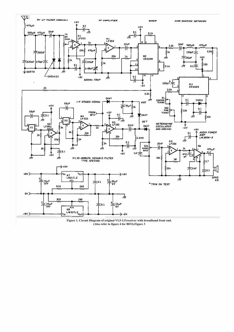
Figure 1. Circuit Diagram of original VLF-LFreceiver with broadband front end.

(Also refer to figure 4 for BFO).Figure 3

The mixer stage

Mixing is carried out by an operational multiplier package type XR2208. This device is suitable for use at frequencies up to 8 MHz, and itsperformance is outstanding as a mixer at low frequencies. Performance tests at an input frequency of 200 kHz and an intermediate frequency (IF) of 455 kHz have produced the following results:

Conversion gain (ratio of output level at 455 kHz to input level at 200 kHz): minus 6 dB.

Equivalent noise level at input: 10 microvolts in a 1-kHz band.

Third-order intermodulation products: At input levels below 70 microvolts, products are below the noise floor. Even at 1-volt input, the third-orderproducts are 55 dB below signal level at 455 kHz.

Level of signal at the output, equal in frequency to the input signal: 33 dB below the level at the input.

Level of signal at the output, equal in frequency to the local oscillator frequency: 53 dB below the level of the oscillator at the mixer input.

The low level of third-order intermodulation products adds up to a low order of nuisance intermodulation beats or "birdies."

The low level of local oscillator signal in the output assists in achieving operation with the oscillator frequency close to the intermediate frequency, as isneeded when tuning at signal frequencies down to 10 kHz.

The tunable local oscillator

For a tunable oscillator, I selected precision oscillator package type XR2209 so variable resistance tuning could be applied. This device can beoperated at frequencies up to 1 MHz, and for an R-C tuned oscillator, has the excellent temperature stability of 20 parts per million per degree Celsius.For the maximum oscillator frequency of 955 kHz required, frequency drift over a 20 degree change is only 360 Hz.

The XR2209 can be connected for either square-wave or triangular-wave output. The latter is fed to the mixer via a sine-shaping filter. The filter isused to reduce the possibility of oscillator harmonics mixing with high level high frequency signals which manage to get through the RF filter at the receiver input and produce unwanted IF beats.

The tuning is carried out by two potentiometers, one for coarse tuning and one for fine tuning. The fixed tuning capacitance and the limitingresistance in series with the two potentiometers are trimmed to obtain an oscillator frequency range of 465 to 955 kHz (455 kHz higher than the tuning range of 10 to 500 kHz). The coarse-tuning potentiometer is connected to a dial which is calibrated in coarse frequency. The values of resistance and capacitance have been selected to suit the full resistance range of the coarse potentiometer. If a vernier dial is used with a shaft rotation of only 180 degrees, the value of limiting resistance can be decreased and the value of fixed capacitance increased to correct for this condition.

RF and IF amplification

To provide RF and IF gain, I used JFET operational amplifier packages type LF353. These are eight-pin DIL packages containing two amplifierswith a 4-MHz gain-bandwidth product. At the frequencies involved, there is a gain of 100 for each package. The RF amplifiers are actually set to realize a gain of 20 per unit at low frequencies, giving a total gain of 400. Of course, this gain decreases at the high frequency end of the tuning range.

One LF353 package is used for RF amplification and one and a half LF353 for IF amplification. The remaining odd half is used as an audio driverfollowing detection.

The RF circuit

The front end of the receiver is broadbanded up to a frequency of around 500 kHz, above which higher frequencies are attenuated by a low-passfilter. The function of the low-pass filter is to reject signals at image frequency which, as it happens, fall within the broadcast band. It also rejects higher frequency signals which could mix with harmonics of the local oscillator to produce a 455-kHz IF beat. The 3dB cutoff point of the filter is set at 500 kHz and its response is 55 dB down at the second harmonic of the cutoff frequency.

A trap circuit is included in the coupling circuit between the two RF amplifier stages. In the first instance, the receiver was made to reject signalsabove 420 kHz and the trap was fitted to reject direct signal pick up at the intermediate frequency. Direct pick up at 455 kHz proved to be no problem. I attribute this to the properties of the XR2208 which balance out the input signals. The receiver could also be tuned across 455 kHz with no undesirable effects. Consequently, I changed the input filter for a cut off frequency of 500 kHz to extend the range of the receiver. The only problem with this change was that it opened up the RF end to signal entry at the extreme end of the broadcast band. Strong local station 5UV on 530 kHz mixed with the second harmonic of the heterodyne oscillator to produce a signal when the receiver was tuned to receive 37.5 kHz. Furthermore, if the RF gain was set too high, 5UV would cross modulate other signals. To eliminate this problem, I set the trap to the 5UV frequency just above 500 kHz.

The IF Circuit

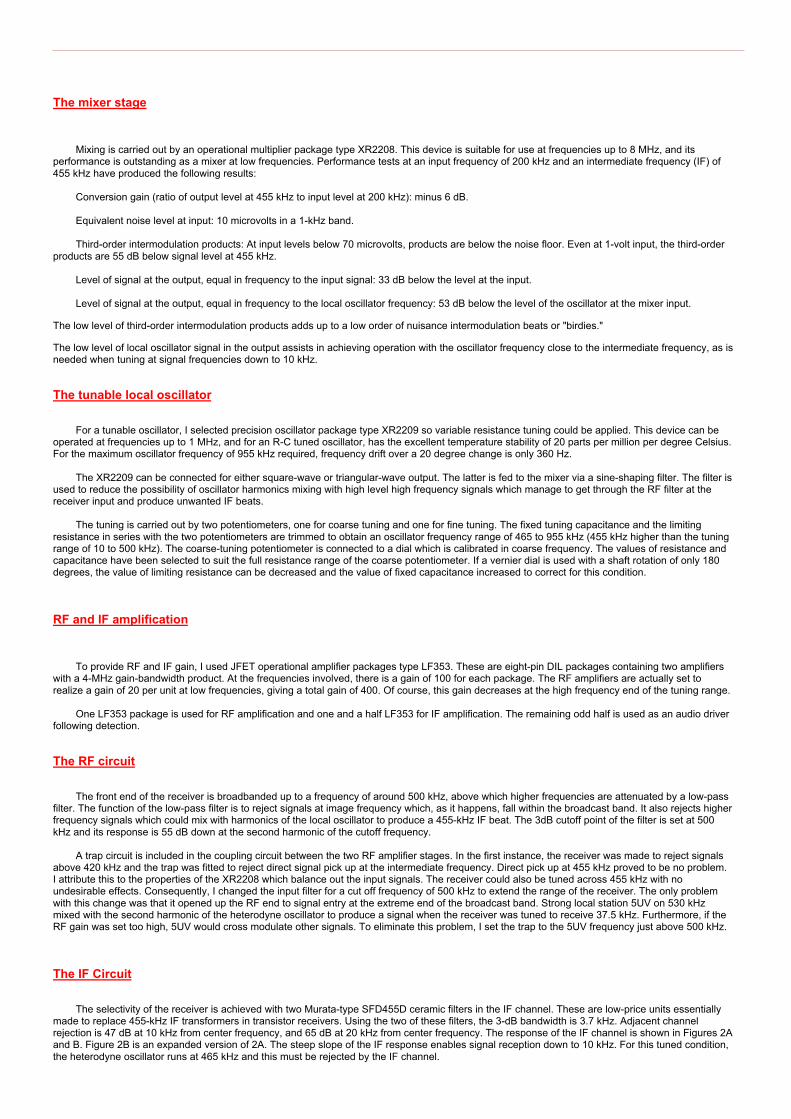
The selectivity of the receiver is achieved with two Murata-type SFD455D ceramic filters in the IF channel. These are low-price units essentiallymade to replace 455-kHz IF transformers in transistor receivers. Using the two of these filters, the 3-dB bandwidth is 3.7 kHz. Adjacent channel rejection is 47 dB at 10 kHz from center frequency, and 65 dB at 20 kHz from center frequency. The response of the IF channel is shown in Figures 2Aand B. Figure 2B is an expanded version of 2A. The steep slope of the IF response enables signal reception down to 10 kHz. For this tuned condition, the heterodyne oscillator runs at 465 kHz and this must be rejected by the IF channel.

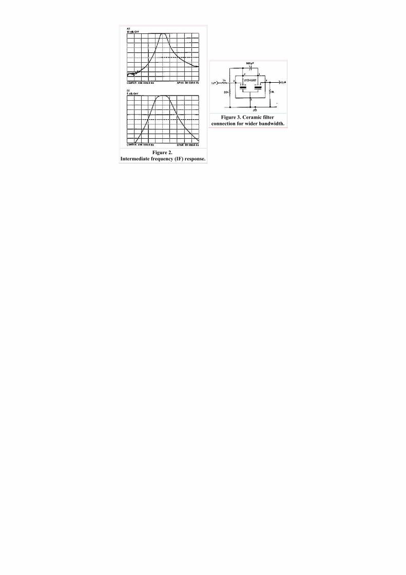
Figure 2.

Intermediate frequency (IF) response.

Figure 3. Ceramic filter

connection for wider bandwidth.

The values of components connected around the filters are as suggested in the manufacturer's brochure. If a wider bandwidth is desired, it canbe achieved by a change in these values. I experimented with one of these filters and found that its bandwidth could be expanded to around 7 kHz by operating with the circuit constants shown in Figure 3.

Audio stages

The IF signal is detected by a diode and following R-C filter. The audio output is fed via the half LF353 preamplifier to an eight pin version of theLM380 power amplifier. The LM380 has internal thermal limiting, and using heat sinking only via the circuit board pins, it can deliver an audio power ofup to 1 watt into a 4-ohm load with a power supply of 9 volts.

Beat frequency oscillator (BFO)

Most of the signals heard within the frequency range transmit in the AM or MCW mode, so the receiver was initially wired up for only that type ofreception. However, there are also CW signals on the bands, like those transmitted by the marine coastal radio, for which a BFO is needed. A BFO is also useful for detecting the presence of some of the navigational signals like Omega. Eventually, I added a BFO. This is shown in Figure 4.

Figure 4. Beat frequency Oscillator (BFO) circuit diagram.

Because the 455-kHz ceramic filters used in the IF stages are quite inexpensive, this provided an impetus to use a third filter for crystal control ofa stable BFO. Tests on the filter showed that a crystal element could be accessed between pin 5 and any of the other pins on the filter, and each element gave a parallel resonance around 456.85 kHz. Pins 1 and 2 elements were found to produce a higher Q than pins 3 or 4 elements.

Another half LF353 was pressed into service to form the oscillator, in conjunction with the ceramic element across pins 1 and 5 and othercomponents as shown in Figure 4. I measured the frequency of oscillation to be 456.36 kHz. This was a satisfactory offset to 455 kHz to operate the incoming signal within the 3.7 kHz IF passband and give a suitable audio frequency beat. The series inductor and shunt capacitor at the amplifier output form a sineshaping filter fitted as a precaution in case harmonics of the BFO caused any problems. The second buffer amplifier is really unnecessary, but I gave it a job to do because it was available as a spare in the LF353 package and required no extra components.

The component values shown to make the circuit oscillate were determined experimentally on a single LF353 and a single ceramic filter. I pointthis out because, in duplicating the circuit, you may find that constants in these devices (particularly the filter) might well vary in different samples, possibly resulting in the need for a change of component values in the feedback path.

Power Rails

Split power rails of plus and minus 6 volts are used for all stages except the audio power amplifier. The split rails enable precise centering ofamplifier operating points making it easy to couple directly, without capacitors, many of the amplifier stages.

The 6-volt rails are derived by voltage regulators type LM317LZ and LM337LZ from a nominal source of plus and minus 9 volts. These very compactregulators are packaged in standard TO-92 transistor cases. The regulators are needed to stabilize the voltage, in particular the voltage to the XR2208oscillator, as its high frequency stability can only be achieved if its power rail voltages are held constant.

Decoupling of the 6-volt rails is used in feeding both oscillator circuits. These are running at a high signal level, and the decoupling is necessaryto prevent coupling into other circuits via the power rails.

The audio power amplifier is powered directly from the positive 9-volt source and does not load the regulator.

The regulated load current is approximately 30 mA per 6-volt rail and is well within the 100mA capacity of the regulators. The additional loadcurrent from the LM380 increases the current on the 9-volt positive supply to 37 mA in the quiescent state and to 134 mA when the power amplifier is driven to its maximum output with continuous sine-wave signal. Under signal conditions, average current is on the order of 50 mA.

The 9-volt power sources can be two small flashlight batteries or twin unregulated DC supplies rectified from a transformed AC supply. If batteriesare used, the positive supply must be shunted with a 2200-uF electrolytic capacitor to prevent the swinging load current of the LM380 from developing a corresponding voltage drop across the battery internal resistance. If the voltage is allowed to swing below 7.7 volts, the regulators cannot do their job and instability occurs. This also puts a limit on how far the batteries can be discharged before the regulated voltage fails. The possibility of instability is eliminated if a separate (third) battery is used for the LM380, so supply to the regulators is unaffected by the LM380 varying load.

Overall sensitivity

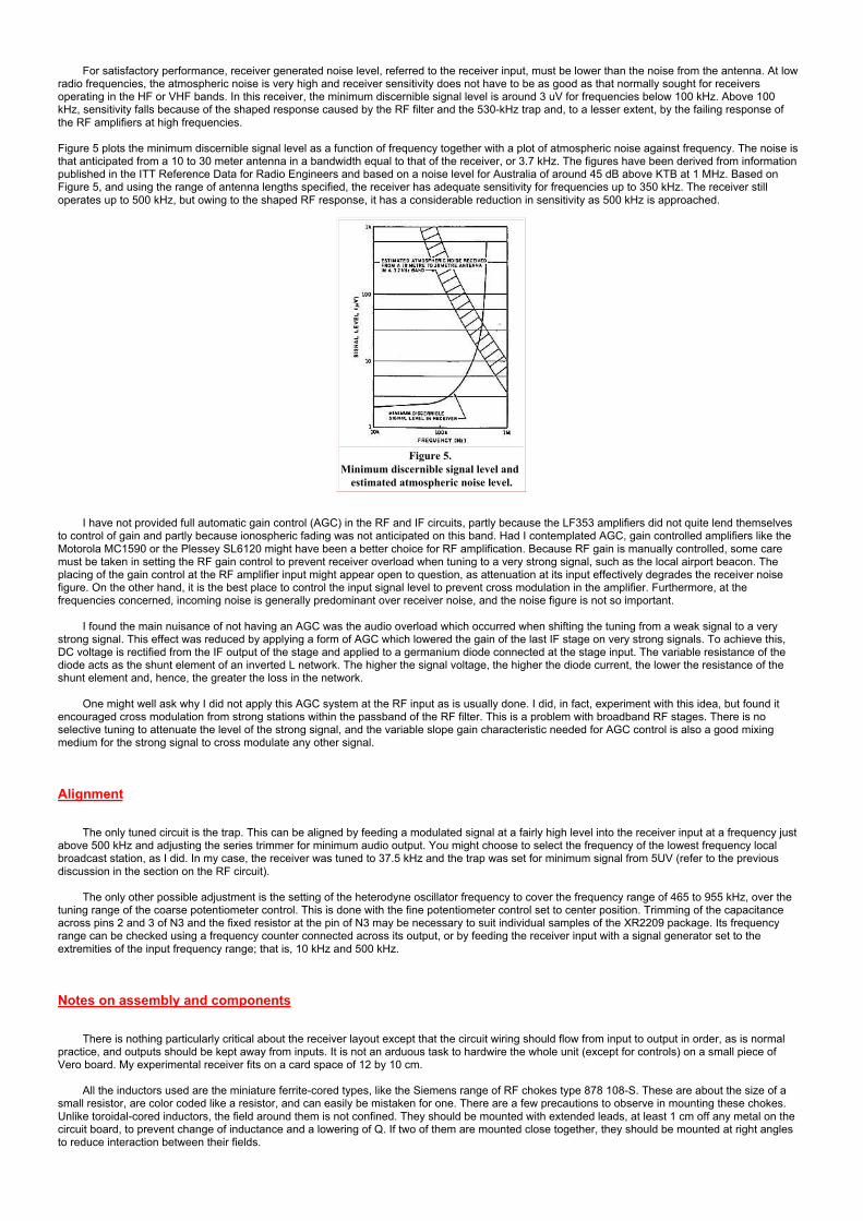
For satisfactory performance, receiver generated noise level, referred to the receiver input, must be lower than the noise from the antenna. At lowradio frequencies, the atmospheric noise is very high and receiver sensitivity does not have to be as good as that normally sought for receivers operating in the HF or VHF bands. In this receiver, the minimum discernible signal level is around 3 uV for frequencies below 100 kHz. Above 100 kHz, sensitivity falls because of the shaped response caused by the RF filter and the 530-kHz trap and, to a lesser extent, by the failing response of the RF amplifiers at high frequencies.

Figure 5 plots the minimum discernible signal level as a function of frequency together with a plot of atmospheric noise against frequency. The noise isthat anticipated from a 10 to 30 meter antenna in a bandwidth equal to that of the receiver, or 3.7 kHz. The figures have been derived from informationpublished in the ITT Reference Data for Radio Engineers and based on a noise level for Australia of around 45 dB above KTB at 1 MHz. Based on Figure 5, and using the range of antenna lengths specified, the receiver has adequate sensitivity for frequencies up to 350 kHz. The receiver still operates up to 500 kHz, but owing to the shaped RF response, it has a considerable reduction in sensitivity as 500 kHz is approached.

Figure 5.

Minimum discernible signal level and

estimated atmospheric noise level.

I have not provided full automatic gain control (AGC) in the RF and IF circuits, partly because the LF353 amplifiers did not quite lend themselvesto control of gain and partly because ionospheric fading was not anticipated on this band. Had I contemplated AGC, gain controlled amplifiers like the Motorola MC1590 or the Plessey SL6120 might have been a better choice for RF amplification. Because RF gain is manually controlled, some care must be taken in setting the RF gain control to prevent receiver overload when tuning to a very strong signal, such as the local airport beacon. The placing of the gain control at the RF amplifier input might appear open to question, as attenuation at its input effectively degrades the receiver noise figure. On the other hand, it is the best place to control the input signal level to prevent cross modulation in the amplifier. Furthermore, at the frequencies concerned, incoming noise is generally predominant over receiver noise, and the noise figure is not so important.

I found the main nuisance of not having an AGC was the audio overload which occurred when shifting the tuning from a weak signal to a verystrong signal. This effect was reduced by applying a form of AGC which lowered the gain of the last IF stage on very strong signals. To achieve this, DC voltage is rectified from the IF output of the stage and applied to a germanium diode connected at the stage input. The variable resistance of the diode acts as the shunt element of an inverted L network. The higher the signal voltage, the higher the diode current, the lower the resistance of the shunt element and, hence, the greater the loss in the network.

One might well ask why I did not apply this AGC system at the RF input as is usually done. I did, in fact, experiment with this idea, but found itencouraged cross modulation from strong stations within the passband of the RF filter. This is a problem with broadband RF stages. There is no selective tuning to attenuate the level of the strong signal, and the variable slope gain characteristic needed for AGC control is also a good mixing medium for the strong signal to cross modulate any other signal.

Alignment

The only tuned circuit is the trap. This can be aligned by feeding a modulated signal at a fairly high level into the receiver input at a frequency justabove 500 kHz and adjusting the series trimmer for minimum audio output. You might choose to select the frequency of the lowest frequency local broadcast station, as I did. In my case, the receiver was tuned to 37.5 kHz and the trap was set for minimum signal from 5UV (refer to the previous discussion in the section on the RF circuit).

The only other possible adjustment is the setting of the heterodyne oscillator frequency to cover the frequency range of 465 to 955 kHz, over thetuning range of the coarse potentiometer control. This is done with the fine potentiometer control set to center position. Trimming of the capacitance across pins 2 and 3 of N3 and the fixed resistor at the pin of N3 may be necessary to suit individual samples of the XR2209 package. Its frequency range can be checked using a frequency counter connected across its output, or by feeding the receiver input with a signal generator set to the extremities of the input frequency range; that is, 10 kHz and 500 kHz.

Notes on assembly and components

There is nothing particularly critical about the receiver layout except that the circuit wiring should flow from input to output in order, as is normalpractice, and outputs should be kept away from inputs. It is not an arduous task to hardwire the whole unit (except for controls) on a small piece of Vero board. My experimental receiver fits on a card space of 12 by 10 cm.

All the inductors used are the miniature ferrite-cored types, like the Siemens range of RF chokes type 878 108-S. These are about the size of asmall resistor, are color coded like a resistor, and can easily be mistaken for one. There are a few precautions to observe in mounting these chokes. Unlike toroidal-cored inductors, the field around them is not confined. They should be mounted with extended leads, at least 1 cm off any metal on the circuit board, to prevent change of inductance and a lowering of Q. If two of them are mounted close together, they should be mounted at right angles to reduce interaction between their fields.

As a general rule, capacitors with a low resistive component should be selected for filters and tuned circuits. This also applies to the filters and trapcircuit in this receiver. Most people choose ceramic capacitors for use in their projects because of their small size, but their resistive component varies from sample to sample in a batch, and it is often quite high. Unless they can be care fully selected for low resistive component using an impedance bridge or Q meter,ceramic capacitors should be avoided if possible. Mica capacitors are good, but are usually much larger. There are some high quality ceramic capacitors, such as the Vitramon VP31 range, but they might be difficult to obtain at the local electronics store.

The only other components which require particular mention are the capacitor and variable resistances used to control the frequency of theheterodyne oscillator. The capacitor across pins 2 and 3 of N3 should be a good stable type (perhaps a mica) and the potentiometers should be noninductive with good resolution. Good quality 1 watt carbon or cermet-type potentiometers will give nice smooth tuning. I emphasize this because there are some very poor potentiometers on the market today, particularly in the miniature variety. One of their faults is the high degree of mechanical backlash which seems to be caused by the elasticity of the bush sealing the shaft. Fortunately, this backlash is steadied when the shaft is loaded down by the reduction gear on a tuning dial.

What can be heard

The VLF and LF bands have their own unique and useful characteristics. It is little affected by reflection from the ionosphere and, because of this,transmission is highly predictable and very useful for direction finding and other forms of radio navigation. Atmospheric attenuation falls as frequency islowered, and given sufficient radiated power, signals at VLF travel large distances around the Earth's surface. A difficulty is the massive aerial system needed to achieve some order of antenna efficiency and, hence, radiated power.

Another limitation is the restricted amount of channel space not suitable for wideband systems. For example, one television channel of around6-MHz bandwidth, on its own, takes up 20 times more band space than the whole of the VLF and LF spectrums put together.

Radio waves are highly attenuated when passing through water, but waves in the VLF region are attenuated the least. (I discussed this in anarticle in the April 1987 issue of Amateur Radio.) Because of the comparatively low attenuation, the VLF band is used for communication to submarines.

Within the Australian region, there are many strong signals transmitted in the VLF and LF band and the part of the MF band tuned by thereceiver. Included in these are the following:

The Omega navigation system can be heard in a frequency band of 10 to 13 kHz. There are actually five different frequencies transmitted which

are switched in a certain order of eight segments in a 10-second time frame. One of the Omega stations is located in Victoria, Australia. (Update: In

more recent times this station has been closed down)

The North West Cape VLF station can be heard with a frequency shift of 100 Hz between 23.25 and 23.35 kHz. (Update: More recently heard

on 19.8 kHz)

A proliferation of aeronautical homing beacons (known as nondirectional beacons or NDBs) within the spectrum of 200 to 420 kHz, transmitcontinuous carrier with Morse ident code. Some also transmit aerodrome control information in voice.

Australian maritime coastal radio stations operate with CW on a range of fixed frequencies between 420 and 490 kHz and listen for merchant

ships on 425, 468, 480, and 512 kHz. The maritime distress frequency is 500 kHz. (Update: Many maritime coastal radio stations have more

recently been closed down.)

A number of Experimental licences have been taken out by individuals for frequencies in the 160 to 200 kHz region. One experimentor, RobertMilne in Tasmania, has been quite active on 177.5 kHz using the call sign AX2TAR.

New Zealand Radio Amateurs have a band allocation of 165 to 190 kHz and these can sometimes be heard in the eastern states of Australia.

Throughout the world, there are several stations in the VLF-LF spectrum which transmit standard time and frequency. GBR (Rugby UK) has beenwell known for its time services on 16 kHz. At low frequencies, these typical signals are ducted around the Earth in a type of wave guide formed by theD layer and the Earth. With a bit of luck, one might pick up some of these.

There are various teletype services which can be heard from time to time. Of course it is difficult to identify who they are unless you can decodetheir signals.

In Europeand northern Asia, frequencies between 150 and 300 kHz are used for long-wave broadcasting. Some of these use very high powerand can sometimes be weakly heard within Australia, particularly below 200 kHz where there is no interference from the local aeronautical beacons.

For those enthusiasts who are interested in short-wave listening and identifying various stations, there is another field of endeavor in long-wavelistening.

Other options

Though I have discussed the design of a complete VLF-LF receiver, there are a few other simple options which might be attractive to othersinterested in these bands. if you have an existing receiver with a 455-kHz IF channel, you could build just the RF end of the receiver described and feed the XR2008 mixer output into the second receiver IF stage via a switch which selects either the VLF-LF front end, or the existing receiver RF end.

Another option is to use the VLF-LF RF end as a converter and feed the mixer output into the second receiver tuned at the low frequency end ofthe broadcast band. A frequency would have to selected clear of strong broadcast carriers, and the connecting lead would have to be carefully shielded. The capacitor across pins 2 and 3 of the XR2209 oscillator would also have to be decreased to shift the oscillator frequencies up a little. Do not try to shift it up too far as the frequency limit of the XR2209 is specified as 1 MHz, although you might get it to operate a little higher than that.

In the receiver described, the IF channel was specifically designed with a narrow bandwidth and a steep out-of-band slope so 10kHz could be tuned. Ifan attached receiver option is used, tuning quite as low as 10 kHz might be restricted if the receiver bandwidth happens to be too wide.

A different type of RF amplifier could easily be used, perhaps with better performance at the MF end of the tuning range. I strongly recommend that you stay with the XR2208 as a mixer because of its balanced mixing type of performance and its low order of intermodulation products.

STAGE 2 - Bandwidth Control

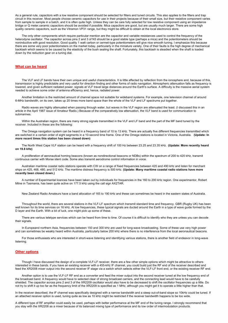
As has been discussed, bandwidth was set at 3.7 kHz by two Murata 455-kHz type SFD455D ceramic filters. This bandwidth is ideal for mediumbandwidth type modes, like AM speech, but is wider than necessary for narrow-band mode signals which exist at frequencies below 100 kHz. These signals are received in the presence of very high noise levels inherent to the LF spectrum and the low end of the VLF spectrum. For these signals, an improvement in signal-to-noise ratio can be achieved by reducing the bandwidth of the receiver. As it turns out, the bandwidth can be narrowed quite simply by switching in a minor circuit change around one of the two ceramic filters.

Curve A of Figure 6 plots the spectral response of the original ceramic filter circuit shown in Figure 7. The bandwidth of the circuit can benarrowed to less than 1 kHz by decreasing the 56-pF inter-filter coupling capacitor to 4.7 pF and terminating the filter in a high impedance. The resulting spectral response is shown by curve B in Figure 6. The high impedance can be achieved by increasing the value of the terminating resistor. However, in the receiver circuit, this resistor is also an input return for the following operational amplifier. Increasing its value without a corresponding change at the amplifier inverting input would affect the DC offset of the amplifier. To avoid changing the inverting input components, I achieved the high impedance by inserting a 4.7-mH choke in series with the original 3-k terminating resistor. The modified circuit for narrow bandwidth is shown in Figure 8.

Figure 6.

(A) Response of the original

wideband filter circuit.

(B) Response of the

narrow-band filter circuit.

Figure 7.

Original wideband filter circuit.

Figure 8.

Narrow bandwidth filter circuit.

Examining again the narrow bandwidth curve B of Figure 6, you will see that it peaks at 457.6 kHz. This works out quite well for centering afrequency to give an audio beat with the beat frequency oscillator (BFO) which is locked at 456.85 kHz. Referring back to Section 1, the BFO was locked by an element in the same type of ceramic filter unit used to control the IF bandwidth.

I found that switching between wide and narrow band, could be achieved easily by switching the inter-filter coupling capacitor between 56 and 4.7pF and leaving the 4.7mH choke in place for both conditions. Figure 9 shows the effect of the choke when leaving it in circuit for the wideband condition. Curve A is the spectral response of the original circuit of Figure 7; curve B is the response with the choke in circuit. It can be seen that the latter condition gives an actual 6-dB gain at the expense of around 3 dB of asymmetrical ripple in the response curve. Whilst the ripple looks untidy on paper, its effect on the practical performance of the receiver is unnoticeable. Furthermore, the 6 dB of gain improvement is also a 6-dB improvement in overall receiver sensitivity, which assists reception at the 500-kHz end of the tuning range where the sensitivity falls away.

Figure 9.

(A) Response of original wideband filter.

(B) Response of wideband filter with

4.7 uH choke left in circuit.

Figure 10.

Filter circuit with wide/narrow

bandwidth switching.

The switchable bandwidth control circuit is shown in Figure 10. This was applied to the first ceramic filter in the IF chain because it was theeasiest one to access on the already wired up board. (The modification could actually be performed without even removing the card from the receiver box.) Of course, there is no reason why the modification could not have been carried out on the second filter, had it been more convenient to achieve. The bandwidth switch was mounted on the receiver front panel and connected into the circuit board via a twisted wire pair. In the circuit shown, the 4.7-pF coupling capacitance for narrowband operation is formed from the series connection of 5.6 and 56 pF. Part of the 5.6-pF capacitance is made up of capacitance in the twisted wire pair to the switch. For wideband operation, the 5.6-pF section is shorted out so the coupling capacitance becomes 56 pF.

Other applications

The bandwidth control circuit was intended specifically for the VLF-LF receiver, but it could well be fitted to any receiver with a 455-kHz IFchannel to improve the reception of narrowband mode signals. Considering its cost and size, the Murata ceramic filter is a very versatile little unit. It can be purchased for but a few dollars. Its dimensions are just 7 x 6 x 7 mm. I have found that by altering the values of source resistance, load resistance, and interfilter coupling capacitance, bandwidth can be set at a range of values between 1 and 7 kHz. Not to be overlooked is the additionalapplication of the filter for crystal control of the beat frequency oscillator.

STAGE 3 - A Front End Tuner

As originally designed, this VLF-LF receiver used a broadband front end. A problem with this type of front end is that it is prone to cross modulationfrom very strong signals or noise outside the tuning bandwidth, but within the broadband range of the front end. When this occurs, it is necessary to reduce the RF input level sufficiently to prevent the problem. However, this also reduces the wanted signal level, possibly well into the noise floor of the receiver. To overcome the problem, I added a front-end tuner.

A further advantage of front-end tuning is that selectivity at VLF can be greatly enhanced. For example, if a Q factor of 200 can be achieved inthe front-end tuned circuit, the bandwidth at 10 kHz is only 10,000/200 = 50 Hz. One of the biggest problems in receiving signals at VLF is the high level of noise, both manmade and atmospheric. The VLF signals, of necessity, are transmitted in narrow-band modes and restriction of bandwidth received is the most effective way to reduce the noise. Furthermore, the narrow bandwidth is also needed to separate some of the signals closely spaced in frequency. All in all, front-end tuning improves the performance of the receiver immensely.

The Front End Tuning System

According to Norm Burton of NSW, who has been experimenting with VI-F reception for at least 25 years, it is very important to tune the aerial atVLF There is certainly nothing wrong in doing just that. However, I have aimed at a tuned-circuit system which is not resonated with the aerial. The reasons for this are as follows:

• Various wire aerials at the home installation, at low frequencies, appear much like a large capacitor in the vicinity of, say, 400 pF against ground. Ifmade part of the tuning system, this residual capacity would have made it difficult to cover the tuning range of 10 to 500 kHz in four bands, as hasbeen done using an ordinary receiver tuning gang.

• An aim in designing the tuner was to make a high Q circuit using a high Q inductor, and it was thought that loss resistance in the Earth system mightrestrict the maximum Q.

*It was also an aim to make the tuning independent of aerial reactance constants, so any aerial could be used.

Generally speaking, I have found that, at low frequencies, the long untuned length of wire gives highest output voltage when loaded into a fairlyhigh resistance. A value of 1000 ohms works quite well, and the original receiver was designed to load the aerial with 1000 ohms. My initial design approach for the tuner was to couple the aerial via a voltage follower stage which presented a high resistance load to the aerial, but drive the tuned circuit in a series mode from its low output resistance to maintain high Q in the tuned circuit. This was unsatisfactory, as the follower stage introduced cross modulation, the very thing which the circuit was supposed to reduce.

The follower stage was ultimately replaced by a low value resistor, which shunts the aerial, but maintains the high Q. This results in voltage lossfrom the aerial, but this loss is more than made up for by voltage magnification in the tuned circuit. (The voltage gain of a tuned circuit is, of course, equal to the value of Q.)

One characteristic of the high Q circuit is that, in the presence of atmospheric static or other transient natured noise, the circuit tends to ring oroscillate on being shocked by the transient impulse. For a given Q, the decay time of oscillation is inversely proportional to frequency. At very low frequencies, this oscillation is detected as an audio ring when using the BFO. Because of this effect, a Q control switch is provided which controls the value of resistance in series with the tuned circuit and hence its Q. The idea is to set the switch for the narrowest bandwidth possible, consistent with atolerable amount of ringing in the presence of noise.

Whilst the circuit design has been based on an untuned aerial, it does not inhibit additional tuning of the aerial circuit to further improveperformance. The option of doing this is dealt with in the section headed "aerials."

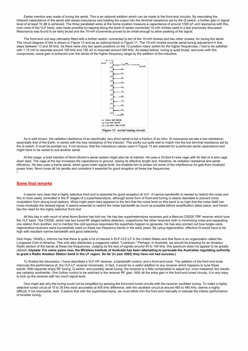
The Tuner Circuit

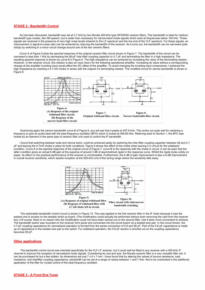
The circuit of the front end tuner is shown in Figure 11. The circuit provides a tunable frequency range of 8 to 600 kHz in four bands switched bySWIB. Other sections of the band switch, SW1A and SW1C, provide direct coupling of the aerial to the receiver for broadband operation when the switch is set to the fifth position.

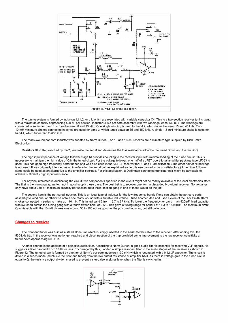
Figure 11. VLF-LF front-end tuner.

The tuning system is formed by inductors LI, L2, or L3, which are resonated with variable capacitor C4. This is a two-section receiver tuning gangwith a maximum capacity approaching 500 pF per section. Inductor Ll is a pot core assembly with two windings, each 130 mH. The windings are connected in series for band 1 to tune between 8 and 25 kHz. One single winding is used for band 2, which tunes between 15 and 40 kHz. Two 10-mH miniature chokes connected in series are used for band 3, which tunes between 35 and 150 kHz. A single 1.5-mH miniature choke is used for band 4, which tunes 140 to 600 kHz.

The ready-wound pot-core inductor was donated by Norm Burton. The 10 and 1.5-mH chokes are a miniature type supplied by Dick SmithElectronics.

Resistors RI to R4, switched by SW2, terminate the aerial and determine the loss resistance added to the tuned circuit and the circuit Q.

The high input impedance of voltage follower stage NI provides coupling to the receiver input with minimal loading of the tuned circuit. This isnecessary to maintain the high value of Q in the tuned circuit. For the voltage follower, one half of a JFET operational amplifier package type LF353 is used. This has good high frequency performance and was also used in the VLF-LF receiver for RF and IF amplification. (The other half of NI package is not used. It was originally intended as an interface for the aerial but, as explained earlier, its use proved to be unsatisfactory.) An emitter follower stage could be used as an alternative to the amplifier package. For this application, a Darlington-connected transistor pair might be advisable to achieve sufficiently high input resistance.

For anyone interested in duplicating the circuit, two components specified in the circuit might not be readily available at the local electronics store.The first is the tuning gang, an item not in good supply these days. The best bet is to recover one from a discarded broadcast receiver. Some gangs only have about 350-pF maximum capacity per section but a three-section gang in one of these would do the job.

The second item is the pot-cored inductor. This is an ideal type of inductor for the low frequency bands if one can obtain the pot-core partsassembly to wind one, or otherwise obtain one ready wound with a suitable inductance. I tried another idea and used eleven of the Dick Smith 10-mH chokes connected in series to make up 110 mH. This tuned band 2 from 15.7 to 67 kHz. To lower the frequency for band 1, an 820-pF fixed capacitor was switched across the tuning gang with a fourth switch bank of SW1. This gave a tuning range for band 1 of 11.3 to 15.9 kHz. The maximum circuit Q achievable with the 10-mH chokes was around 50 to 100 not as good as the potcored inductor, but still quite good.

Changes to receiver

The front-end tuner was built as a stand alone unit which is simply inserted in the aerial feeder cable to the receiver. After adding this, the530-kHz trap in the receiver was no longer required and disconnection of the trap provided some improvement to the low receiver sensitivity at frequencies approaching 500 kHz.

Another change is the addition of a selective audio filter. According to Norm Burton, a good audio filter is essential for receiving VLF signals. Hesuggests a filter bandwidth of 100 Hz or less. Encouraged by this, I added a simple resonant filter to the audio stages of the receiver as shown in Figure 12. The tuned circuit is formed by another of Norm's pot-core inductors (130 mH) which is resonated with a 0.12,uF capacitor. The circuit is driven in a series mode (much like the front-end tuner) from the low output resistance of amplifier N5B. As there is voltage gain in the tuned circuit equal to Q, the resistive output divider is used to prevent a steep rise in signal level when the filter is switched in.

Figure 12.

Addition of 1200 Hz audio filter to the receiver.

The frequency of the filter is 1200 Hz, worked out as follows: In the narrow IF mode, the center frequency is 457.6 kHz. The BFO is needed toreceive the narrowband modes. This runs at 456.4 kHz, 1200 Hz lower than the intermediate center frequency. Hence, maximum signal beat occurs ata frequency of 1200 Hz, and this is the tuned frequency of the filter. The bandwidth of the filter is 100 Hz, and it is very effective in reducing much of the low frequency hash which gets through in spite of the narrow RF bandwidth.

Operation of the Tuner in conjunction with the Receiver

Operation of the front-end tuner in conjunction with the receiver can be a little tricky, as the front end is not ganged to the receiver tuning. Onemethod of tuning is to set the band switch to the broadband position and first locate the station with the receiver tuning dial. The band switch is then set to the appropriate band and the tuning gang is set for maximum signal level. Care must be taken not to tune in to the frequency of a strong signal which would simply enhance cross modulation by that signal. Tuning on the lowest frequency bands is very sharp, and on the unit constructed, a 2.5:1reduction gear was fitted to the tuning knob to assist in adjustment. A calibrated scale marked in frequency for each band was also added to simplify setting of the front-end tuning near the frequency marked on the receiver tuning dial. With this aid, the front-end tuning is then simply trimmed for peaksignal level with little chance of false tuning.

A problem at VLF-LF is noise from mains operated equipment in the local vicinity, particularly in one's own house. I find it necessary to turn offfluorescent lamps, triac controlled light dimmer switches, and TV sets. The TV line time base at 15625 Hz, in the middle of the VLF band, is a particular nuisance. This type of noise tends to disappear after midnight, when everyone has switched things off and gone to bed.

Measured Performance of the Tuner

Table 1 lists measurements taken of bandwidth and Q for various frequencies in each band of the tuner and with Q set maximum. It is interestingto observe the high Q factors obtained, particularly for bands 1 and 2 which use the pot core. This is something which could not be achieved in the early days, before ferrite cores, unless regeneration was applied.

Table 2 lists measurements taken of bandwidth and Q at 15 kHz on band 1 for different settings of the Q switch. This shows that a 6:1 range ofbandwidth and Q can be selected.

BandFrequency

kHz

Bandwidth

HzQ

1 10 48 208

1 15 60 250

1 20 84 238

1 25 132 189

2 16 85 188

2 25 121 207

2 35 234 150

3 40 610 66

3 70 802 87

3 120 1140 105

3 150 1360 110

4 150 1830 82

4 200 3480 57

4 300 2910 103

4 400 2300 174

Table 1. Bandwidth "Q" position 1.

Switch

Pos

Bandwidth

HzQ

1 60 250

2 83 181

3 145 103

4 226 66

5 360 42

Table 2. Bandwidth for different "Q" switch positions. At 15 kHz on band 1.

Aerials

At low frequencies the usual wire aerial is but a fraction of a wavelength long and, as a general rule, the more wire put up in the air, the greaterthe signal level captured. As one would expect, at the home location the longest of three wire aerials available gives the highest signal level. The signal level is also improved by about 6 dB when all three wires are paralleled together.

Earlier mention was made of tuning the aerial. This is an optional addition which can be made to the front-end circuitry. By resonating theinherent capacitance of the aerial with series inductance and loading the output into the terminal resistance set by the Q switch, a further gain in signallevel of at least 10 dB is achieved. The three paralleled wires at the home location measure a capacitance of around 1000 pF and resonance with this,over most of the VLF band, was made possible by tapping along the bank of series connected 10-mH chokes used in a test previously discussed. Resonance was found to be fairly broad and the 10-mH increments proved to be small enough to allow peaking of the signal.

The front-end unit was ultimately fitted with a further switch, connected to ten of the 10-mH chokes and two other chokes, for tuning the aerial.The circuit diagram of this is shown in Figure 13 and as an optional block in Figure 11. The 10-mH chokes provide aerial tuning adjustment in fine steps between 13 and 50 kHz. As there were only two spare positions on the 12 position rotary switch for the higher frequencies, I had to be satisfied with 1.15 mH to resonate around 150 kHz and 150 uH to resonate around 400 kHz. As stated before, tuning is quite broad, and even with this compromise, some gain is achieved over the whole of the higher frequency range by the addition of the inductors.

Figure 13. Aerial tuning circuit.

As is well known, the radiation resistance of an electrically very short aerial is but a fraction of an ohm. At resonance we see a low resistance,essentially that of the Earth, in series with the loss resistance of the inductor. This works out quite well to match into the low terminal resistance set by the Q switch. It must be pointed out, if not obvious, that the inductance values used in Figure 13 are selected for a particular aerial capacitance and might have to be varied to suit another aerial.

At this stage, a brief mention of Norm Burton's aerial system might also be of interest. He uses a 33-foot 6~wire cage with 42 feet of 4-wire cagedown lead. The cage at the top increases the capacitance to ground, raising its effective length and, therefore, its radiation resistance and aerial efficiency. He also uses a frame aerial, which gives lower signal level, but enables him to phase out some of the interference he gets from localized power lines. Norm tunes all his aerials and considers it essential for good reception at these low frequencies.\

Some final remarks

It seems very clear that a highly selective front end is essential for good reception at VLF. A narrow bandwidth is needed to restrict the noise andthis is more easily controlled in the IF stages of a superheterodyne, although some form of front-end tuning is clearly desirable to prevent cross modulation from strong local stations. What might seem less apparent is the fact that the noise level on this band is so high that the noise itself can cross-modulate the desired signal. It seems essential to restrict the noise bandwidth as much as possible before amplification takes place, and herein lies the need for the highly selective front end.

All this ties in with much of what Norm Burton has told me. He has two superheterodyne receivers and a Marconi CR200 TRF receiver which tunethe VLF band. The CR200, which has two tuned RF stages before detection, outperforms the other receivers both in minimizing noise and separating one station from another, not to mention the odd spurious responses the superhets happen to generate. He has also pointed out how single-valve regenerative receivers were successfully used on these low frequency bands in the early years. By using regeneration, effective Q would have to be high with resultant narrow bandwidth and good selectivity.

Dick Hope, VK4DLJ, informs me that there is quite a lot of interest in ELF-VLF-LF in the United States and that there is an organization called theLongwave Club of America. This club also distributes a magazine called, "Lowdown." Perhaps, in Australia, we should be pressing for an Amateur Radio section of the bands at these low frequencies. Judging by the lack of signals around 40 to 100 kHz, this spectrum does not appear to be greatly

utilized. (Update: For some years now, the Wireless Institute of Australia has been attempting to persuade the Australian regulating authority

to grant a Radio Amateur Station band in the LF region. So far (in year 2002) they have not had success.)

To finalize the discussion, I have described a VLF-HF receiver, a bandwidth control, and a front-end tuner. The addition of the front end tunerimproves the performance of, the VLF-LF receiver immensely. In fact, it would be a useful addition to any receiver which happens to tune these bands. With separate sharp RF tuning, Q switch, and possibly aerial tuning, the receiver is a little complicated to adjust but, once mastered, the resultsare certainly worthwhile. One further control to be watched is the receiver RF gain. With all the extra gain in the front-end tuned circuits, it is very easy to lock up the receiver with too much signal level.

One might ask why the tuning could not be simplified by sensing the front-end tuned circuits with the receiver oscillator tuning. To make a highlyselective tuned circuit at 10 to 30 kHz track accurately at 455 kHz difference, with the oscillator circuit at around 465 to 485 kHz, seems a highly difficult, if not impossible, task. It seems that with the superheterodyne, we must either trim the front end manually or tolerate the inferior performance of broader tuning.

Receiver on right, with Front End Tuner lower left,

and Loop Tuner top left

Back to HomePage