Vladimir Andrić* Milojko Arsić Aleksandra Nojković* · PDF fileutilize panel data sets, due to the relatively short time coverage for transition economies. Second, we detect

47

ECONOMIC ANNALS, Volume LXI, No. 210 / July – September 2016UDC: 3.33 ISSN: 0013-3264

* PhD Candidate in Economics, Faculty of Economics, University of Belgrade, Republic of Serbia, Email: [email protected]

** Faculty of Economics, University of Belgrade, Republic of Serbia Email: [email protected]

*** Faculty of Economics, University of Belgrade, Republic of Serbia, Email: [email protected]

1 We wish to express our deepest gratitude to two anonymous referees whose valuable comments improved the quality of the paper significantly. We also thank, without implication, Boyan Jovanovic, Michel Habib, Miloš Božović, Zorica Mladenović and Branko Urošević for excellent comments on previous versions of this paper. The standard disclaimer applies.

DOI:10.2298/EKA1610047A

Vladimir Andrić*Milojko Arsić**Aleksandra Nojković***

PUBLIC DEBT SUSTAINABILITY IN SERBIA BEFORE AND DURING THE GLOBAL FINANCIAL CRISIS1

JEL CLASSIFICATION: C54, H63, P20

ABSTRACT: We have analyzed the be-haviour of primary fiscal balance and public debt in Serbia before and in the af-termath of the global financial crisis. The results of our analysis are: i) public debt to GDP ratioexhibits (near) unit root behav-iour with an overall upward time trend; ii) the response of primary fiscal balance to public debt has been insufficient to mean revert the upward trend in government debt; iii) the efforts of the Serbian govern-ment to repay the debt principal after the fiscal rule breach have not been persistent,

providing empirical support to the fiscal fa-tigue hypothesis; iv) the government budget constraint has deteriorated since the begin-ning of the global financial crisis; v) the re-sponse of primary fiscal balance to public debt from the onset of the global financial crisis has dropped more severely in com-parison to other European economies.

KEY WORDS: Serbia, unit root tests, fis-cal reaction functions, global financial cri-sis.

1. INTRODUCTION

In this paper we analyse the behaviour of primary fiscal balance and public debt in Serbia before and during the global financial crisis. Our analysis addresses four main research questions. First, does the trajectory of public-debt-to-GDP ratio satisfy government budget constraint, i.e., is the Serbian public-debt-to-GDP ratio sustainable? Second, does primary fiscal balance respond to public debt accumulation? Third, is the behaviour of the Serbian government consistent with the fiscal fatigue hypothesis? Fourth, has the budget constraint of the Serbian government deteriorated more since the beginning of the global financial crisis?

The results of our analysis are: i) the trajectory of public-debt-to-GDP ratio exhibits (near) unit root behaviour with an overall upward time trend, i.e., the Serbian public-debt-to-GDP ratio is unsustainable; ii) the response of primary fiscal balance to public debt accumulation has been insufficient to mean revert the upward trend in government debt; iii) the efforts of the Serbian government to repay the debt principal after the fiscal rule breach have not been persistent, providing empirical support for the fiscal fatigue hypothesis; and iv) the government budget constraint has deteriorated since the beginning of the global financial crisis as from its onset the response of primary fiscal balance to public debt accumulation has dropped more severely than in other European economies.

Our analysis covers the period from 2004Q3 to 2014Q3, so it does not take into account the fiscal consolidation package initiated in 2014Q4. In analysing the behaviour of primary fiscal balance and public debt in Serbia we complement the use of unit root tests with ordinary least squares (OLS) estimates of fiscal reaction functions (FRFs). We estimate a broad range of FRFs, both linear and non-linear, with particular emphasis on the structural break due to the global financial crisis.

Our empirical estimates add several contributions to the existing body of knowledge on the behaviour of primary fiscal balance and public debt. First, our research is one of the first papers to analyse the behaviour of primary fiscal balance and public debt in the case of Serbia. We present a detailed single country study using time series data, while most other studies in the literature

48

Economic Annals, Volume LXI, No. 210 / July – September 2016

utilize panel data sets, due to the relatively short time coverage for transition economies. Second, we detect a change in the fiscal behaviour of the Serbian government following a fiscal rule breach. The government took corrective action, but the effort was insufficient to reverse the upward trajectory of public debt. Third, the Serbian government is one of the rare European governments that has not implemented fiscal consolidation measures from the onset of the global financial crisis, at least in the period we analyse. The estimates of FRFs with breakpoints show how the budget constraint of the Serbian government deteriorated more heavily than in other European economies.

The rest of the paper is organized as follows. Section II acquaints the reader with major trends in Serbian public finances before and during the global financial crisis. Section III derives the government budget constraint. Section IV presents the results of the unit root tests. Section V outlines our empirical estimates of FRFs, and Section VI concludes.

2. DATA AND TRENDS

Our empirical analysis covers the period between 2004Q3 and 2014Q3, so it does not take into account the fiscal consolidation package initiated in 2014Q4. Two distinctive sub-periods characterize our sample span: the first covers the period from 2004Q3 to 2008Q3 and the second covers the period from 2008Q4 to 2014Q3.

In the first sub-period the public-debt-to-GDP ratio declined by approximately 30 percentage points. Between 2002 and 2005 the government, supported by the IMF’s Extended Arrangement, carried out a fiscal consolidation package of over 5% of GDP (Cocozza et al. 2011), recording a fiscal surplus in 2005. In addition, externally fuelled rapid economic growth, absorption-gap-caused buoyancy in government revenues, and debt write-offs by the Paris and London club of creditors pushed government debt as a percentage of GDP further downward. Between 2006 and 2008 the government, funded by massive privatization revenues, embarked on a journey of procyclical fiscal expansion. The adoption of a five-year National Investment Plan, public sector wage increases, and a cut in the marginal tax rate on wages accompanied by an increase in non-taxable wage threshold created a structural fiscal imbalance in Serbian public finances in this two-year period. In 2008 the Serbian government also adopted a trade

PUBLIC DEBT SUSTAINABILITY IN SERBIA

49

agreement with the EU which assumed a reduction in customs rates on imported goods, resulting in an overall loss of customs revenue equal to around 1.5% of GDP.

The Serbian government continued its expansionary fiscal policy at the beginning of our second sub-period. In particular, in the wake of the global financial crisis, unprecedented hikes in public sector wages and pensions of around 2.5% of GDP, along with the sharp decline in government revenues, caused further deterioration in the fiscal balance. At the beginning of 2009 the Serbian government responded to its deteriorating fiscal policy stance by freezing public wages and pensions2 during 2009 and 2010, introducing a tax on mobile services, increasing excise taxes on oil and oil derivatives, and reducing agricultural subsidies, subsidies to state-owned enterprises, and transfers to local governments. These measures resulted in a relatively lower average fiscal deficit of 4.5% of GDP between 2009 and 2010 in comparison to new EU member states from Central and Eastern Europe, which recorded an average fiscal deficit of 6% of GDP in the same period. Most of the implemented measures were, however, only temporary (public wages and pensions freeze, tax on mobile services etc.), and the Serbian government abandoned them in 2011. In addition, in mid-2011 the government adopted a fiscal decentralization package which created vertical fiscal imbalances of approximately 1.7% of GDP (Arsić et al. 2012). The government also rescued several state-owned banks and enterprises in 2012 and 2013. Therefore, between 2011 and 2014 the fiscal deficit in Serbia was increasing and amounted, on average, to 5.9% of GDP, while in other emerging European economies the fiscal deficit constituted only 3.4% of GDP in the same period, as a direct consequence of introduced fiscal austerity measures. The Serbian government started implementing systematic austerity measures in 2014Q4, several years later than other European economies.

Consequently, deteriorating fiscal balance pushed the public-debt-to-GDP ratio upwards by approximately 40 percentage points between 2008Q3 and 2014Q3 –from 30% of GDP in 2008Q3 to 68% of GDP in 2014Q3. The growth of Serbian

2 The average annual inflation rate in 2009 and 2010 was 8.4%, so the nominal freeze of public

wages and pensions significantly contributed to the reduction of government spending and overall fiscal deficit in real terms.

50


public liabilities represents one of the fastest increases in government indebtedness among emerging European economies.

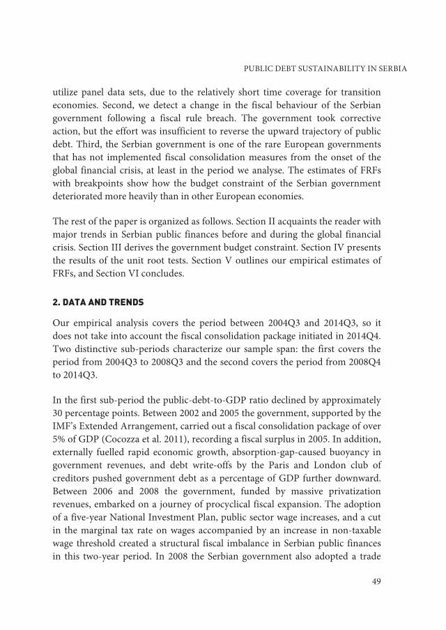
At the end of 2014 the public-debt-to-GDP ratio in emerging European economies constituted, on average, around 52% of GDP. Serbia’s public debt corresponds to more than 70% of its GDP, as depicted in Figure 1 below. Figure 1 also documents how Croatia, Hungary, and Albania were the only countries with higher public-debt-to-GDP ratios among emerging European economies at the end of same year.

Figure 1: General Government Gross Debt (% of GDP) in Emerging European Economies at the end of 2014

Source: IMF WEO, April 2015

The deterioration of the primary fiscal balance from the onset of the global financial crisis contributed the most to the upward trend of Serbian public debt. Between 2008Q4 and 2010Q4 primary fiscal balance fluctuated around its mean value of -3.5% of GDP, while between 2011Q1 and 2014Q3 it averaged around -3.1% of GDP. Hence the overall fiscal balance breached its medium-run bound of -1% of GDP, defined in fiscal rules as about 3.5 percentage points, on average. We document these trends in Figure 2, in which we depict the dynamics of

0

10

20

30

40

50

60

70

80

90

CRO HUN ALB SRB MNE POL BIH ROU MKD TUR BGR

% of GDP


51

seasonally adjusted primary fiscal balance and public debt in Serbia between 2004Q3 and 2014Q3.3

Figure 2: Primary Fiscal Balance (% of GDP) and Public Debt (% of GDP) in Serbia, 2004Q3-2014Q3

Sources: Ministry of Finance and the Statistical Office of the Republic of Serbia

From the standpoint of public debt stability, the currency composition of Serbian public debt is unfavourable, since the Serbian government has issued 80% of its debt in foreign currency. In addition, the Serbian dinar is sensitive to net capital flows. High current account deficits, accompanied by the sudden cessation of capital inflows and higher capital outflows triggered by the global financial crisis, caused the dinar to lose approximately 20% of its value between October 2008 and March 2009. In particular, given the Serbian public debt level of around 75% of GDP, if the dinar depreciates by 1 percentage point in

3 We use a data set that comprises official time series data from Ministry of Finance, the

National Bank of Serbia, and the Statistical Office of the Republic of Serbia. We follow ESS guidelines (Eurostat 2015) in implementing the TRAMO/SEATS procedure to seasonally adjust the data. All data, both seasonally unadjusted and adjusted, is available from the authors upon request.

52


nominal terms the public-debt-to-GDP ratio increases by, on average, 0.6 percentage points. A sensitive exchange rate, coupled with one of the most euroized economic systems in Central and Eastern Europe, can create additional contingent liabilities for the Serbian government.

The maturity structure of Serbian government debt might also cause problems regarding public debt risk management. In particular, at the end of 2014 only 14.4% of total dinar-denominated government debt had a maturity longer than 3 years, while the corresponding share for euro-denominated government debt was 27.5% (Ministry of Finance 2015). The maturity composition of Serbian public debt, although favourable from the standpoint of total interest burden, bears significant rollover risks.

According to Baldacci et al. (2011), the probability of fiscal crisis in emerging economies increases if, among other things, the following scenarios emerge: i) the cyclically adjusted primary fiscal balance exceeds a threshold of around -0.5% of GDP; ii) general government gross debt exceeds a threshold of around 43% of GDP; and iii) foreign-currency-denominated public debt constitutes more than approximately 40% of total government debt. Even if the results of Baldacci et al. (2011) do not hold with certainty, Maastricht Convergence Criteria stipulate the following conditions for Serbia’s formal accession to the European Union: i) a public-debt-to-GDP ratio below 60%; ii) an overall fiscal balance above -3% of GDP; and iii) stability of exchange rate fluctuations and the convergence of domestic interest rates towards the overall level of interest rates in the European Union. Given the trends in Serbian public finances documented above, we cannot rule out a fiscal crisis in Serbia in the coming years.

3. GOVERNMENT BUDGET CONSTRAINT

Since the seminal work of Hamilton and Flavin (1986), government budget constraint can be used as a theoretical framework for the empirical application of unit root tests in analysing public debt sustainability. Hence in this section we follow Hamilton and Flavin (1986) and Bohn (2007).


53

The value of public debt at time t is:

�� (III.1)

in which �� represents non-interest government expenditure, �� represents government revenue, �� represents interest rate, and �� represents public debt from the previous period.4

The difference

�� (III.2)

is the overall fiscal deficit, since �� represents overall government expenditure. The difference �� is primary, non-interest, fiscal deficit. If we shift (III.1) one period ahead and assume constant interest rates5, the difference equation for the public debt becomes

�� (III.3)

in which � � � �� ⁄ � � � � represents a deterministic discount factor. Recursive substitutions forward yield the expected present value condition for the public debt

�� ∑ �� (III.4)

4 If the variables are measured in nominal terms, �� represents nominal interest rate. If the

variables are measured in real terms, �� represents real interest rate. If the variables are measured in GDP shares, �� represents the interest rate (nominal or real) minus the growth rate (nominal or real). In the case of Serbia, �� represents the weighted average of domestic and foreign interest rates adjusted for exchange-rate-induced valuation gains or losses. For details, see Bohn (2007, page 1839).

5 The constancy of interest rates is the most common assumption in the literature. Two other assumptions are: i) interest rates are uncorrelated over time with positive and constant conditional expectation �� ii) interest rates follow any stationary stochastic process with mean �� . Both assumptions lead to the difference equation (II.3). For details, see Bohn (2007, pages 1838-1840).

54


in which discounted expected future primary fiscal balances finance current public debt obligations. Government budget constraint holds if the transversality condition

(III.5)

holds. Since creditors do not tolerate the bubble build-up in public debt, the transversality condition represents the no-Ponzi game condition in public debt sustainability analysis.

The expected present value condition and transversality condition are equivalent conditions (Bohn, 2007). They are consistent with the increasing stock of debt, as long as the rate of public debt increase is less than the interest rate (Hamilton and Flavin 1986). In other words, the government does not have to pay off its entire debt.

To nest the null and alternative hypotheses for subsequent unit root testing and following Hamilton and Flavin (1986), we write the government debt valuation equation in its most general form

(III.6)

The null hypothesis �� is

(III.7)

The alternative hypothesis �� is

(III.8)

Hamilton and Flavin (1986) argue that if �� is stationary, for any stationary process ∑ �� On the other

hand, if then �� is nonstationary. Stated differently, if public debt follows a stationary stochastic process, then the transversality condition holds and public debt is sustainable. On the other hand, if the


55

transversality condition does not hold, then public debt follows a nonstationary stochastic process and hence public debt is unsustainable.

If public debt is integrated of order �, ��, for any finite�� , then public debt satisfies the transversality condition, and debt, revenue, and expenditure satisfy government budgetary constraint (Bohn 2007). The n-period-ahead conditional expectation of an mth-order integrated stochastic process for �� is at most an mth-order polynomial of time horizon n.6 The discounting in the transversality condition is the exponential function of n. The exponential growth dominates polynomial growth of any order. In other words, government budget constraint holds regardless of the order of integration for the public debt process. Hence testing for the unit root in public debt becomes meaningless. The analysis is valid only in the long run, i.e., for infinite-horizon government budget constraint. In the short-to-medium run, the distinction between the stationary and nonstationary stochastic processes for public debt has economic importance, because nonstationary public debt can violate any upper bound that policymakers may impose (Bohn 2007). Since Serbian public debt in 2012Q1 violated the 45% of GDP upper bound defined in fiscal rules, in the next section we apply a battery of unit root tests.

4. DEBT SUSTAINABILITY TESTS

In interpreting the results of the unit root tests we adopt the criterion of Uctum et al. (2006), who considered trending public debt in finite samples to be sustainable if and only if the underlying data generating process (DGP) was negative trend stationary. A downward-sloping trend does not have to imply the dynamic inefficiency of the government in finite samples, while stationarity provides the predictability of DGP.

We present the results of an augmented Dickey-Fuller (ADF) unit root test (Dickey and Fuller 1981) in the first row of Table 1. Serbian public debt is on an unsustainable path, since we fail to reject a random walk with positive drift null hypothesis for public-debt-to-GDP ratio between 2004Q3 and 2014Q3. We scale public debt with GDP, since: i) GDP share is the most appropriate measure for growing economies, as Hakkio and Rush (1991) indicate; and ii) market

6 For details, see proposition 1 in Bohn (2007, page 1840).

56


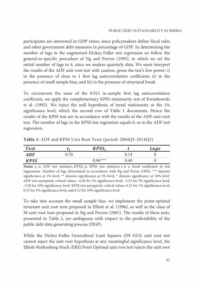
participants are interested in GDP ratios, since policymakers define fiscal rules and other government debt measures in percentage of GDP. In determining the number of lags in the augmented Dickey-Fuller test regression we follow the general-to-specific procedure of Ng and Perron (1995), in which we set the initial number of lags to 4, since we analyse quarterly data. We must interpret the results of the ADF unit root test with caution, given the test’s low power: i) in the presence of close to 1 first lag autocorrelation coefficient; ii) in the presence of small sample bias; and iii) in the presence of structural break.

To circumvent the issue of the 0.912 in-sample first lag autocorrelation coefficient, we apply the complementary KPSS stationarity test of Kwiatkowski et al. (1992). We reject the null hypothesis of trend stationarity at the 1% significance level, which the second row of Table 1 documents. Hence the results of the KPSS test are in accordance with the results of the ADF unit root test. The number of lags in the KPSS test regression equals 0, as in the ADF test regression.

Table 1: ADF and KPSS Unit Root Tests (period: 2004Q3-2014Q3)

-0.76 - 0.14 0

- 0.96*** 0.40 0 Notes: is ADF test statistics, is KPSS test statistics, is a trend coefficient in test regressions. Number of lags determined in accordance with Ng and Peron (1995). *** denotes significance at 1% level, ** denotes significance at 5% level, * denotes significance at 10% level. ADF test asymptotic critical values: -4.20 for 1% significance level, -3.53 for 5% significance level, -3.20 for 10% significance level. KPSS test asymptotic critical values: 0.22 for 1% significance level, 0.15 for 5% significance level, and 0.12 for 10% significance level.

To take into account the small sample bias, we implement the point-optimal invariant unit root tests proposed in Elliott et al. (1996), as well as the class of M-unit root tests proposed in Ng and Perron (2001). The results of these tests, presented in Table 2, are ambiguous with respect to the predictability of the public debt data generating process (DGP).

While the Dickey-Fuller Generalized Least Squares (DF GLS) unit root test cannot reject the unit root hypothesis at any meaningful significance level, the Elliott-Rothenberg-Stock (ERS) Point Optimal unit root test rejects the unit root


57

hypothesis at more than a 1% significance level. In addition, modified Phillips-Perron tests, and , cannot reject the unit root hypothesis, but the opposite is true for modified ERS point optimal test and modified Sargan-Bhargava test .

Table 2: Sample Bias and Unit Root Tests (period: 2004Q3-2014Q3)

-0.63 Trend & Intercept 1 MAIC

30.31*** Trend & Intercept 1 MAIC -2.76 Trend & Intercept 1 MAIC -0.98 Trend & Intercept 1 MAIC 27.26*** Trend & Intercept 1 MAIC 0.35*** Trend & Intercept 1 MAIC

Notes: *** denotes significance at 1% level, ** denotes significance at 5% level, * denotes significance at 10% level. Number of lags in each test determined in accordance with the modified AIC (MAIC), as in Ng and Perron (2001). Long-run HAC corrected variance in each test obtained with GLS detrended autoregressive spectral density estimator, as in Ng and Perron (2001).

To take into account the structural break in public debt, we implement the Zivot-Andrews endogenous structural break unit root test (Zivot and Andrews 1992). We test the no-break random walk null hypothesis against all three stationarity alternatives embodied in: i) model A, which incorporates a structural break in the level of the series; ii) model B, which incorporates a structural break in the trend of the series; iii) model C, which incorporates structural breaks in both the level and the trend of the series.

We outline estimation results in Table 3. The results from Table 3 favour model B, although Model C describes public debt dynamics almost as well as Model B. Model B rejects the null hypothesis at more than a 1% significance level, and dates the break in 2008Q3. Model C rejects the unit root null hypothesis at a 10% significance level, and dates the break in 2008Q2. In estimating each test specification, we determine the number of lags as in Ng and Perron (1995). We discriminate between the three test specifications by comparing their respective standard errors (S.E.), the values of the Akaike (AIC), Schwarz (SIC), and Hannan-Quinn (HQIC) information criteria.

58


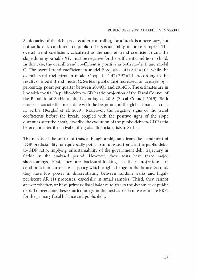
Stationarity of the debt process after controlling for a break is a necessary, but not sufficient, condition for public debt sustainability in finite samples. The overall trend coefficient, calculated as the sum of trend coefficient and the slope dummy variable , must be negative for the sufficient condition to hold. In this case, the overall trend coefficient is positive in both model B and model C. The overall trend coefficient in model B equals -1.45+2.52=1.07, while the overall trend coefficient in model C equals -1.47+2.57=1.1. According to the results of model B and model C, Serbian public debt increased, on average, by 1 percentage point per quarter between 2004Q3 and 2014Q3. The estimates are in line with the 83.5% public-debt-to-GDP ratio projection of the Fiscal Council of the Republic of Serbia at the beginning of 2018 (Fiscal Council 2015). Both models associate the break date with the beginning of the global financial crisis in Serbia (Berglöf et al. 2009). Moreover, the negative signs of the trend coefficients before the break, coupled with the positive signs of the slope dummies after the break, describe the evolution of the public-debt-to-GDP ratio before and after the arrival of the global financial crisis in Serbia.

The results of the unit root tests, although ambiguous from the standpoint of DGP predictability, unequivocally point to an upward trend in the public-debt-to-GDP ratio, implying unsustainability of the government debt trajectory in Serbia in the analysed period. However, these tests have three major shortcomings. First, they are backward-looking, so their projections are conditional on current fiscal policy which might change in the future. Second, they have low power in differentiating between random walks and highly persistent AR (1) processes, especially in small samples. Third, they cannot answer whether, or how, primary fiscal balance relates to the dynamics of public debt. To overcome these shortcomings, in the next subsection we estimate FRFs for the primary fiscal balance and public debt.


59

Table 3: Zivot-Andrews Unit Root Test (period: 2004Q3-2014Q3)

Notes: Values in the tZA column are the values of Zivot-Andrews test statistic. Values in columns t, DU and DT are coefficients for trend, shift level dummy and slope dummy. Associated t -statistics are given in ( ). The number of lags determined as in Ng and Perron (1995). *** denotes significance at 1% level, ** denotes significance at 5% level, * denotes significance at 10% level. Asymptotic critical values for 1%, 5% and 10% significance level are: model A: -5.34, -4.80, -4.58; model B: -4.93, -4.42, -4.11; model C: -5.57, -5.08 and -4.82.

5. FISCAL REACTION FUNCTIONS

FRFs quantify the response of primary fiscal balance to changes in public debt. Bohn (1998) claims how a positive, at least linear, statistically significant response of primary fiscal balance to public debt accumulation is sufficient to imply mean reversion in a stochastic process for public debt. Bohn’s argumentation for estimating FRFs is twofold. First, the unit root testing of government budget constraint relies on simplifying assumptions about the behaviour of interest rates. In particular, the constancy of interest rates implies risk-neutral private investors. FRFs in Bohn (1998), on the other hand, do not depend on interest rates. Second, unit root test regressions are prone to omitted variable bias, since they are not grounded in any theoretical framework of fiscal policy behaviour. FRFs in Bohn (1998), however, stem from Barro’s (1979) tax-smoothing model. In this model, policymakers first set the level of permanent government spending. Exogenous permanent government spending determines the level of collected tax revenue. In collecting taxes, the government fixes the tax rate to minimize the administrative costs of tax collection and the deadweight cost of taxation incurred by the taxpayers. Consequently, transitory government spending, as a consequence of wars, political and business cycles, and output gap, via its impact on the tax base, are the only non-debt

3.94

3.74

3.80

4.05

3.88

3.97

3.88

3.66

3.71

1.61

1.42

1.44

0

1

1

-

2.52 (5.24)

2.57 (5.04)

-5.17 (-4.04)

-

-2.97 (-2.03)

0.25 (6.75)

-1.45 (-4.81)

-1.47 (-4.74)

-3.41

-5.4***

-4.98*

2006Q1

2008Q3

2008Q2

A

B

C

60


determinants of the primary fiscal balance. The expected sign of transitory government spending on primary fiscal balance is negative, while the expected sign of output gap on primary fiscal balance is positive.

Following Bohn (1998), we estimate the following OLS regression:

�� (V.1)

in which �� represents primary fiscal balance, �� is lagged public debt, �� is transitory government spending, �� is output gap, and �� are i.i.d. normal white noise residuals with parameters � and ��. ��is a dummy variable which equals 1 if� � ��, and 0 otherwise. All regressors are in % of GDP, except ��, which is in log levels, as in Uctum et al. (2006). We compute �� as the detrended values of nominal government expenditure, and then divide the corresponding transitory component by nominal GDP. ��is calculated by detrending the values of log real GDP.7 According to the results of the unit root tests, the process for �� is trend-stationary, so we do not test for the cointegration between �� and ��.8 We present the coefficient estimates from equation (V.1) in Table 4 below. Table 4 shows how the estimated response of primary fiscal balance to a 1-percentage point increase in public debt is 0.05 percentage points. The estimated response is significant at more than 1% significance level. We use lagged public debt as an explanatory variable for two reasons. First, we circumvent potential correlation between contemporaneous public debt and the unexplained variations of primary fiscal balance. Second, we allow the additional quarter for the corrective fiscal actions of the government in repaying the debt principal. Although the positive response of primary fiscal balance to public debt in Table 4 implies mean reversion in the stochastic process for public debt, we must analyse the magnitude of the estimated response in connection with the results of the unit root tests from the previous subsection. The estimated response of 0.05 percentage points in

7 We use Hodrick-Prescott (HP) filter with smoothing parameter set to 1,600 in both

calculations. 8 The first lag autocorrelation coefficient for �� equals 0.512. The ADF test rejects the random

walk with a drift unit root hypothesis at more than 1% significance level. The results are available from the authors upon request.


61

Table 4 is insufficient to mean revert the public-debt-to-GDP ratio in the short-to-medium run, given the 1.07 percentage point estimate for the overall debt trend coefficient in Table 3.

The global financial crisis has increased the share of primary fiscal deficit in GDP by 3.65 percentage points, as the estimated coefficient for the dummy variable ��in Table 4 indicates. Transitory government spending and output gap also have the expected signs and a satisfactory statistical significance. In particular, the percentage point increase (decrease) of general government expenditure as % of GDP from its overall trend level reduced (increased) the share of primary fiscal balance in GDP by 0.91 percentage points. In addition, the percentage point increase (decrease) of real GDP from its potential level increased (reduced) the share of primary fiscal balance in GDP by 0.11 percentage points. The estimation results are robust with respect to the Newey-West correction. The results are also robust with respect to the simultaneity bias between primary fiscal balance on the one hand and transitory government spending and output gap on the other, since the respective correlations with the residuals in equation (V.1) are indistinguishable from zero. Our estimates do not change even when we instrument ��with its lagged value. The instrument is not weakly identified, since the Cragg-Donald F-statistic equals 13.69. In addition, the Hausman simultaneity test cannot reject the exogeneity of output gap at the 13% significance level.9 We have also experimented with additional explanatory variables, most notably with contemporaneous and lagged trade balance, inflation rate, and lagged primary fiscal balance. Trade balance and its lagged value fail to capture the effect of absorption gap on primary fiscal balance through the impact on government revenue, most probably because output gap and global financial crisis have already encompassed it. We have also omitted inflation rate from the final specification, since its effect has been statistically insignificant. Lagged primary fiscal balance fails to capture the persistence in the stochastic process for��, so it does not figure in equation (V.1) and Table 4.

9 We have also experimented with potential instruments for transitory government spending,

but we believe there is no relevant economic rationale which might explain the influence of primary fiscal balance on transitory government spending on a quarterly basis, particularly for the period we consider and under the theoretical foundations on which we base our empirical estimates.

62


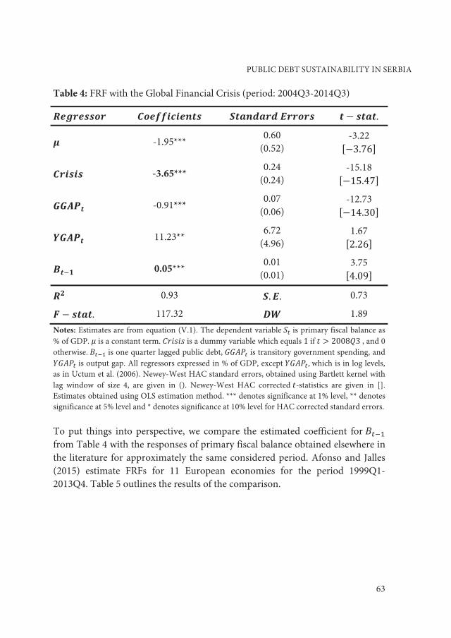
Table 4: FRF with the Global Financial Crisis (period: 2004Q3-2014Q3)

�� .

� -1.95*** 0.60

(0.52) -3.22

��.�6� �� -3.65***

0.24 (0.24)

-15.18 ��1�.4��

�� -0.91*** 0.07

(0.06) -12.73

��14.�0� �� 11.23**

6.72 (4.96)

1.67 �2.26�

�� 0.05*** 0.01

(0.01) 3.75 �4.09�

�� 0.93 �. �. 0.73

� � ��. 117.32 �� 1.89 Notes: Estimates are from equation (V.1). The dependent variable �� is primary fiscal balance as % of GDP. � is a constant term. �� is a dummy variable which equals 1 if � � 200��, and 0 otherwise. �� is one quarter lagged public debt, �� is transitory government spending, and �� is output gap. All regressors expressed in % of GDP, except ��, which is in log levels, as in Uctum et al. (2006). Newey-West HAC standard errors, obtained using Bartlett kernel with lag window of size 4, are given in (). Newey-West HAC corrected �-statistics are given in []. Estimates obtained using OLS estimation method. *** denotes significance at 1% level, ** denotes significance at 5% level and * denotes significance at 10% level for HAC corrected standard errors.

To put things into perspective, we compare the estimated coefficient for �� from Table 4 with the responses of primary fiscal balance obtained elsewhere in the literature for approximately the same considered period. Afonso and Jalles (2015) estimate FRFs for 11 European economies for the period 1999Q1-2013Q4. Table 5 outlines the results of the comparison.


63

Table 5: Cross-Country Comparison of FRFs

Austria Belgium Finland France Germany Greece Ireland Italy Netherlands Portugal Spain Serbia

0.010 NO 0.152*** YES

0.077 NO 0.096*** YES 0.127** YES

0.031 NO 0.136 NO 0.059 NO

0.296*** YES 0.017 NO 0.061 NO

0.05*** NO Notes: Estimates for 11 European economies for the period 1999Q1-2013Q4 are from Afonso and Jalles (2015), Table 4, page 15. Estimates for Serbia for the period 2004Q3-2014Q3 are authors’ calculations. *** denotes significance at 1% level, ** denotes significance at 5% level and * denotes significance at 10% level for HAC corrected standard errors.

Estimates from Table 5 indicate how fiscal policy is sustainable in Belgium, France, Germany, the Netherlands, and Serbia, since the response of primary fiscal balance to public debt accumulation is positive and statistically significant. This finding becomes more intuitive when we take into account the presence of the long-run cointegrating relationship between primary fiscal balance and public debt in Belgium, France, Germany, and the Netherlands. Primary fiscal balance and public debt have the same degree of persistence in these countries. Moreover, they co-move in a synchronized manner towards long-run equilibrium. Afonso and Jalles (2015) confirm this result both with the Johansen-Juselius procedure and with the dynamic ordinary least squares method of Stock, Watson, and Shin. In Serbia, however, the process for public debt exhibits (near) unit root behaviour, while the process for primary fiscal balance belongs to a class of stationary stochastic processes. Hence shocks to public debt are more persistent than shocks to primary fiscal balance. In other words, changes in public debt have a more lasting effect in the system than changes in primary fiscal balance. To shed more light on this issue, we proceed in two directions. First, we investigate whether and how the response of primary

64


fiscal balance changes when public debt accelerates towards higher debt levels. Second, we investigate whether and how the response of primary fiscal balance changes when, due to an exogenous crisis shock, debt reverses its trend from downward-sloping to upward-sloping.

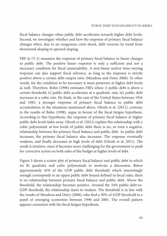
FRF in (V.1) measures the response of primary fiscal balance to linear changes in public debt. The positive linear response is only a sufficient and not a necessary condition for fiscal sustainability. A non-linear and/or time-varying response can also support fiscal solvency, as long as the response is strictly positive above a certain debt-output ratio (Mendoza and Ostry 2008). In other words, for the condition to be necessary it must persevere at higher debt levels as well. Therefore, Bohn (1998) estimates FRFs when: i) public debt is above a certain threshold; ii) public debt accelerates at a quadratic rate; iii) public debt increases at a cubic rate. He finds, in the case of the United States between 1916 and 1985, a stronger response of primary fiscal balance to public debt accumulation in the situations mentioned above. Ghosh et al. (2011), contrary to the results of Bohn (1998), argue in favour of the fiscal fatigue hypothesis. According to this hypothesis, the response of primary fiscal balance at higher public debt levels fades away. Ghosh et al. (2011) explain this relationship with a cubic polynomial: at low levels of public debt there is no, or even a negative, relationship between the primary fiscal balance and public debt. As public debt increases, the primary fiscal balance also increases. The response eventually weakens, and finally decreases at high levels of debt (Ghosh et al. 2011). The result is intuitive, since it becomes more challenging for the government to push for corrective action on both sides of the budget at higher levels of debt.

Figure 3 shows a scatter plot of primary fiscal balance and public debt in which we fit quadratic and cubic polynomials to motivate a discussion. Below approximately 45% of the GDP public debt threshold, which interestingly enough corresponds to an upper public debt bound defined in fiscal rules, there is no relationship between primary fiscal balance and public debt. Above the threshold, the relationship becomes positive. Around the 54% public-debt-to-GDP threshold, the relationship starts to weaken. The threshold is in line with the results of Mendoza and Ostry (2008), who find a 50%-of-GDP threshold in a panel of emerging economies between 1990 and 2005. The overall pattern appears consistent with the fiscal fatigue hypothesis.


65

Figure 3: Scatterplot of Public Debt and Primary Fiscal Balance with Polynomial Fits in Serbia, 2004Q3-2014Q3

Source: Authors’ calculations

We estimate three additional FRFs to explore stylized facts from the data. First, following Plödt and Reicher (2014) and Snower et al. (2011), we estimate a FRF with ��∗ public debt variable in which��∗ equalsmax�� . We opt for a 45%-of-GDP threshold because of the upper public debt bound defined in fiscal rules. We do not experiment with higher public-debt-to-GDP ratios because of the insufficient number of sample points corresponding to the values above certain thresholds. Second, following Bohn (1998), we estimate a FRF with quadratic polynomial in public debt. Third, following Mendoza and Ostry (2008) and Ghosh et al. (2011), we estimate a FRF with cubic polynomial in public debt.

-8

-6

-4

-2

0

2

4

6

24 28 32 36 40 44 48 52 56 60 64

Lagged Public Debt (% of GDP)

Prim

ary

Fisc

al B

alan

ce (%

of G

DP

)

Quadratic PolynomialCubic Polynomial

Fiscal Rule Breach

66


Table 6 outlines the estimation results. The first column shows the results from estimating FRF with 45%-of-GDP public debt threshold. The second column shows the results of estimating FRF with a quadratic polynomial in public debt. The third column shows the results from estimating FRF with a cubic polynomial in public debt. We caution the reader to interpret the estimation results carefully due to potential overfitting and multicollinearity issues.

The results are, however, consistent with the patterns in Figure 3. The estimated coefficient for�� in the first column of Table 6 is statistically insignificant and equals 0.01, while the estimated coefficient for��∗ is significant at the 10% level and equals 0.08. Hence the government takes additional corrective action when the public-debt-to-GDP ratio exceeds the 45% threshold. The government signals to creditors how it implements fiscal adjustment measures when faced with a fiscal rule breach. In comparison to our baseline estimates from Table 4, the response of primary fiscal balance to public debt accumulation strengthens by only 0.03 percentage points after the fiscal rule breach. Hence the response is still insufficient to mean revert the accelerating debt dynamics, given the estimates of the overall debt trend coefficient in Table 3. The absence of stronger corrective government action can jeopardize future fiscal consolidations, since the magnitude of adjustment, along with its expected persistence, is the most important characteristic of successful fiscal consolidation, at least according to Giavazzi and Pagano (1990).

The coefficient for �� from the second column of Table 6, statistically significant at the 5% level, equals only 0.002, implying almost no response of primary fiscal balance at higher debt levels. In addition, the coefficient for �� from the third column of Table 6, significant at the 10% level, is indistinguishable from zero, providing further evidence in favour of the fiscal fatigue hypothesis in the case of Serbia.10 In other words, changes in primary fiscal balance cannot keep pace with changes in public debt when the debt accelerates towards higher debt levels.

10 We have also estimated FRFs with reduced quadratic and cubic polynomials. The response of

primary fiscal balance to �� equals 0.0006, significant at 1% level. The response of primary fiscal balance to �� equals 0.000009, significant at 1% level. The results are available from the authors upon request.


67

Table 6: FRFs with Debt Fatigue (period: 2004Q3-2014Q3)

��

� -0.56 (1.05) [0.99]

2.63 (2.37) [2.07]

14.75* (8.66) [7.56]

�� -3.72*** (0.24) [0.22]

-3.76*** (0.24) [0.21]

-3.69*** (0.24) [0.24]

�� -0.91*** (0.07) [0.06]

-0.91*** (0.069) [0.060]

-0.91*** (0.068) [0.06]

�� 7.24

(7.03) [5.62]

6.58 (6.86) [5.62]

6.76 (6.76) [5.98]

�� 0.01

(0.027) [0.027]

-0.16* (0.11) [0.09]

-1.07* (0.63) [0.54]

�� 0.002** (0.0012) [0.0010]

0.024* (0.015) [0.012]

�� -0.000164*

(0.0001) [0.00009]

��∗ 0.08*

(0.047) [0.043]

�� 0.93 0.93 0.93 �� 0.71 0.70 0.69 �� 2.03 2.06 2.11 �� 2.30 2.26 2.25 �� 2.55 2.51 2.54 �� 2.40 2.35 2.35 Notes: ��-primary fiscal balance as % of GDP is the dependent variable. �-constant term; ��-dummy variable which equals 1 if � � ��, and 0 otherwise; ��-transitory government spending; �� -output gap;�� -lagged public debt; ��∗ -max�� . All regressors expressed in % of GDP, except �� , which is in log levels as in Uctum et al. (2006). ()-ordinary standard errors; []-Newey-West HAC standard errors, with Bartlett lag window of 4. OLS estimation method. *** significance at 1% level, ** significance at 5% level and * significance at 10% level for HAC corrected standard errors.

68


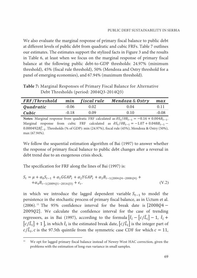
We also evaluate the marginal response of primary fiscal balance to public debt at different levels of public debt from quadratic and cubic FRFs. Table 7 outlines our estimates. The estimates support the stylized facts in Figure 3 and the results in Table 6, at least when we focus on the marginal response of primary fiscal balance at the following public debt-to-GDP thresholds: 24.97% (minimum threshold), 45% (fiscal rule threshold), 50% (Mendoza and Ostry threshold for a panel of emerging economies), and 67.94% (maximum threshold).

Table 7: Marginal Responses of Primary Fiscal Balance for Alternative Debt Thresholds (period: 2004Q3-2014Q3)

�� -0.06 0.02 0.04 0.11 �� -0.18 0.09 0.10 -0.08 Notes: Marginal response from quadratic FRF calculated as �� ⁄ � �0.1� � 0.004��. Marginal response from cubic FRF calculated as �� ⁄ � �1.0� � 0.04�� 0.0004�2�� . Thresholds (% of GDP): min (24.97%), fiscal rule (45%), Mendoza & Ostry (50%), max (67.94%).

We follow the sequential estimation algorithm of Bai (1997) to answer whether the response of primary fiscal balance to public debt changes after a reversal in debt trend due to an exogenous crisis shock.

The specification for FRF along the lines of Bai (1997) is:

in which we introduce the lagged dependent variable �� to model the persistence in the stochastic process of primary fiscal balance, as in Uctum et al. (2006). 11 The 95% confidence interval for the break date is �200��4 �200��2� . We calculate the confidence interval for the case of trending regressors, as in Bai (1997), according to the formula ��̂� � �� 1� �̂� �� 1�� in which �̂� is the estimated break date, �� is the integer part of ��, � is the 97.5th quintile from the symmetric case CDF for which � � 11� 11 We opt for lagged primary fiscal balance instead of Newey-West HAC correction, given the

problems with the estimation of long-run variance in small samples.

�� 0��1 � �1�� 2�� 3��1�2004�4�200��4� ��4��1�200��1�2014�3� � �� . (V.2)


69

and is a scale factor with , and defined as the public debt coefficient before the break point, public debt coefficient after the break point, and the estimated variance of from (V.2), respectively. The use of symmetric CDF is appropriate, since the model’s residuals are stationary on the whole sample. The results of both the ADF and KPSS test confirm this finding.12

We outline the results of the estimation in Table 8. The budget constraint of the Serbian government has deteriorated more since the onset of the global financial crisis. For the period before the break, the average response of primary fiscal balance to a 1 percentage point increase in public debt equaled 0.15 percentage points. The response is statistically significant at more than 1% significance level. For the period after the break, the average response has dropped to 0.05 percentage points. The response is again significant at more than 1% significance level. Hence the responsiveness of primary fiscal balance to public debt accumulation has diminished since the beginning of the global financial crisis. The drop in response is primarily due to: the 2008 trade agreement with the EU that resulted in a loss of customs revenue of around 1.5% of GDP; hikes in public wages and pensions of around 2.5% of GDP in the wake of the global financial crisis; a recession-induced automatic sharp decline in government revenue due to the global financial meltdown; fiscal decentralization measures from 2011 that created vertical fiscal imbalances of approximately 1.7% of GDP; and the government bailout of several state-owned banks and enterprises in 2012 and 2013. Hence the size of the discrepancy between the two estimated coefficients shows the lack of fiscal consolidation measures in Serbia after the outbreak of the global financial crisis.

12 The ADF test statistic with intercept equals -5.02, while the corresponding KPSS test statistic

equals 0.08. The results are available from the authors upon request.

70


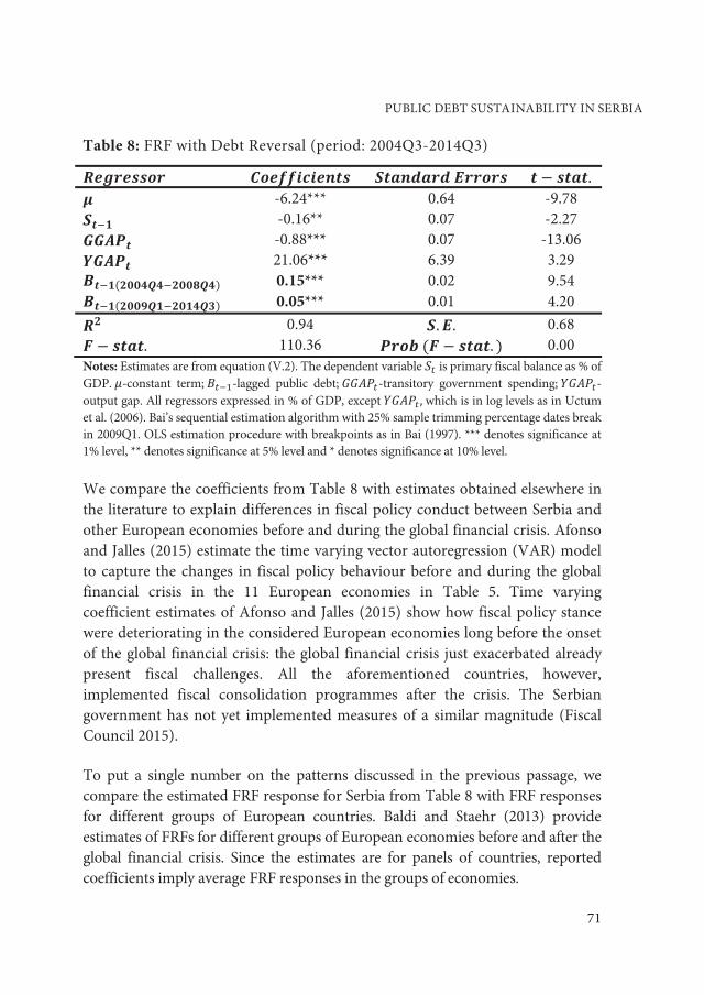
Table 8: FRF with Debt Reversal (period: 2004Q3-2014Q3)

�� -6.24*** 0.64 -9.78 �� -0.16** 0.07 -2.27 �� -0.88*** 0.07 -13.06 �� 21.06*** 6.39 3.29 �� 0.15*** 0.02 9.54 �� 0.05*** 0.01 4.20 �� 0.94 �� 0.68 � � �� 110.36 �� 0.00 Notes: Estimates are from equation (V.2). The dependent variable �� is primary fiscal balance as % of GDP. �-constant term; ��-lagged public debt; ��-transitory government spending; ��-output gap. All regressors expressed in % of GDP, except ��, which is in log levels as in Uctum et al. (2006). Bai’s sequential estimation algorithm with 25% sample trimming percentage dates break in 2009Q1. OLS estimation procedure with breakpoints as in Bai (1997). *** denotes significance at 1% level, ** denotes significance at 5% level and * denotes significance at 10% level.

We compare the coefficients from Table 8 with estimates obtained elsewhere in the literature to explain differences in fiscal policy conduct between Serbia and other European economies before and during the global financial crisis. Afonso and Jalles (2015) estimate the time varying vector autoregression (VAR) model to capture the changes in fiscal policy behaviour before and during the global financial crisis in the 11 European economies in Table 5. Time varying coefficient estimates of Afonso and Jalles (2015) show how fiscal policy stance were deteriorating in the considered European economies long before the onset of the global financial crisis: the global financial crisis just exacerbated already present fiscal challenges. All the aforementioned countries, however, implemented fiscal consolidation programmes after the crisis. The Serbian government has not yet implemented measures of a similar magnitude (Fiscal Council 2015).

To put a single number on the patterns discussed in the previous passage, we compare the estimated FRF response for Serbia from Table 8 with FRF responses for different groups of European countries. Baldi and Staehr (2013) provide estimates of FRFs for different groups of European economies before and after the global financial crisis. Since the estimates are for panels of countries, reported coefficients imply average FRF responses in the groups of economies.


71

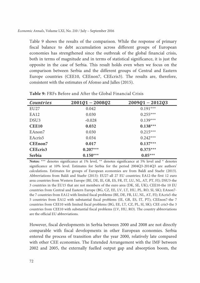
Table 9 shows the results of the comparison. While the response of primary fiscal balance to debt accumulation across different groups of European economies has strengthened since the outbreak of the global financial crisis, both in terms of magnitude and in terms of statistical significance, it is just the opposite in the case of Serbia. This result holds even when we focus on the comparison between Serbia and the different groups of Central and Eastern Europe countries (CEE10, CEEnon7, CEEcris3). The results are, therefore, consistent with the estimates of Afonso and Jalles (2015).

Table 9: FRFs Before and After the Global Financial Crisis

EU27 0.042 0.191*** EA12 0.030 0.255*** DSU3 -0.028 0.139*** CEE10 0.032 0.138*** EAnon7 0.030 0.215*** EAcris5 0.034 0.242*** CEEnon7 0.017 0.137*** CEEcris3 0.207*** 0.375*** Serbia 0.150*** 0.05*** Notes: *** denotes significance at 1% level, ** denotes significance at 5% level and * denotes significance at 10% level. Estimates for Serbia for the period 2004Q3-2014Q3 are authors’ calculations. Estimates for groups of European economies are from Baldi and Staehr (2013). Abbreviations from Baldi and Staehr (2013): EU27-all 27 EU countries; EA12-the first 12 euro area countries from Western Europe (BE, DE, IE, GR, ES, FR, IT, LU, NL, AT, PT, FI); DSU3-the 3 countries in the EU15 that are not members of the euro area (DK, SE, UK); CEE10-the 10 EU countries from Central and Eastern Europe (BG, CZ, EE, LV, LT, HU, PL, RO, SI, SK); EAnon7-the 7 countries from EA12 with limited fiscal problems (BE, DE, FR, LU, NL, AT, FI); EAcris5-the 5 countries from EA12 with substantial fiscal problems (IE, GR, ES, IT, PT); CEEnon7-the 7 countries from CEE10 with limited fiscal problems (BG, EE, LT, CZ, PL, SI, SK); CEE cris3-the 3 countries from CEE10 with substantial fiscal problems (LV, HU, RO). The country abbreviations are the official EU abbreviations.

However, fiscal developments in Serbia between 2000 and 2008 are not directly comparable with fiscal developments in other European economies. Serbia entered the process of transition after the year 2000, relatively late compared with other CEE economies. The Extended Arrangement with the IMF between 2002 and 2005, the externally fuelled output gap and absorption boom, the

72


public debt write-offs by the London and Paris club of creditors, and the use of privatization proceeds for deficit financing represent the main reasons why fiscal policy stance in Serbia appeared sustainable before the crisis. These developments, however, led policymakers to conduct procyclical expansionary fiscal policy, thus creating the structural discrepancy between government revenue and expenditure between 2006 and 2008. 13 It would be more appropriate, therefore, to compare the results for Serbia with FRF estimates for other Western Balkan economies. Koczan (2015) and Baldi and Staehr (2013) give the unavailability of time series data as the most important reason for the lack of such studies. The comparisons we have made, however, are not completely groundless. Lewis (2013) documents how fiscal loosening in CEE economies started between 1999 and 2001, especially after the Nice Treaty had been agreed upon in 2001. Von Hagen and Wolff (2006) make an even stronger claim: advanced European economies engaged in creative accounting practices by covering large fiscal deficits with stock-flow adjustments after the Stability and Growth Pact was agreed upon in 1998. Hence Serbia is not the only European economy in which non-economic factors have determined the behaviour of fiscal policy from the year 2000 onward.

6. CONCLUSION

We have analysed the behaviour of primary fiscal balance and public debt in Serbia before and during the global financial crisis. Our findings can be summarized as follows. First, public-debt-to-GDP ratio exhibited (near) unit root behaviour with an overall upward time trend between 2004Q3 and 2014Q3, i.e., the trajectory of the Serbian public-debt-to-GDP ratio is unsustainable in the analysed period. The Extended Arrangement with the IMF, externally fuelled output gap and absorption boom, and debt write-offs by the Paris and London club of creditors caused government debt as percentage of GDP to decline between 2004Q3 and 2008Q3. However, between 2006 and 2008, when the Serbian economy experienced rapid expansion, policymakers simultaneously cut taxes and increased government spending, which resulted in high structural fiscal deficit. In addition, in the wake of the global financial

13 The emergence of a structural fiscal deficit took place in the first half of 2006, immediately

after the Extended Arrangement with the IMF had expired, pointing to the weakness of fiscal institutions in Serbia during the transition period.


73

crisis, when government revenue declined sharply, policymakers increased public wages and pensions by approximately 2.5% of GDP. In 2009 and 2010 the government adopted a package of fiscal consolidation measures: a public wages and pensions freeze, several tax hikes, and simultaneous spending cuts, which resulted in relatively lower average fiscal deficit in comparison to other emerging European economies during the global financial crisis. However, most of these measures were temporary and were ended by the government in 2011. Moreover, in mid-2011 the government adopted fiscal decentralization measures which created vertical fiscal imbalances of around 1.7% of GDP. The government also bailed out several state-owned banks and enterprises in 2012 and 2013, thus failing to implement systematic fiscal austerity measures. Consequently, between 2011 and 2014 the fiscal deficit in Serbia increased with respect to its average level during the global financial crisis between 2009 and 2010. Overall, fiscal consolidation measures adopted in the aftermath of the global financial crisis between 2011 and 2014 were unable to mean revert the upward public debt trajectory. Second, we have confirmed the relevance of fiscal fatigue hypothesis in the case of Serbian public debt. The Serbian government increased its efforts to repay the debt principal after the fiscal rule breach in 2012Q1. The effort, however, has not been persistent, since the government has failed to contain the accelerating public debt dynamic. Third, the response of primary fiscal balance to public debt accumulation has dropped sharply since the onset of the global financial crisis. The drop in this response is more severe than in other European economies. Both panel and time series evidence from the literature available to us support this claim.

The Serbian government launched a massive 3-year fiscal consolidation package in 2014Q4. Our analysis does not take into account these fiscal developments. Although the primary fiscal balance improved significantly in 2015, future analyses must wait additional data to evaluate whether the trajectory of public-debt-to-GDP ratio has been reversed. Consequently, a detailed investigation of how to restore the responsiveness of primary fiscal balance to public debt accumulation is the most important research priority from a policymaking perspective.

74



75

REFERENCES

Afonso, A. & Jalles, J.T. (2015). Euro Area Time Varying Fiscal Sustainability. (WP13/2015/DE/UECE), Lisbon: Lisbon School of Economics and Management.

Arsić, M., Nojković, A., Randjelović, S. & Micković, S. (2012). Strukturni fiskalni deficit i dinamika javnog duga Srbije. Beograd, Republika Srbija: Ekonomski fakultet, Univerzitet u Beogradu.

Bai, J. (1997). Estimation of a Change Point in Multiple Regression Models. The Review of Economics and Statistics, 79 (4), pp. 551-563. DOI: 10.1162/003465397557132.

Baldacci, E., Petrova, I., Belhocine, N., Dobrescu, G. & Mazraani, S. (2011). Assessing Fiscal Stress. (IMF Working Paper WP/11/100), Washington D.C.: International Monetary Fund.

Baldi, G. & Staehr, K. (2013). The European Debt Crisis and Fiscal Reaction Functions in Europe 2000-2012. (DIW Berlin Discussion Paper 1295), Berlin: German Institute for Economic Research.

Barro, R. (1979). On the Determination of the Public Debt. Journal of Political Economy, 87 (5), pp. 940-971. DOI: 10.1086/260807.

Berglöf, E., Korniyenko, Y., Plekhanov, A. & Zettelmeyer, J. (2009). Understanding the Crisis in Emerging Europe. (EBRD Working Paper No. 109), London: European Bank for Reconstruction and Development.

Bohn, H. (2007). Are Stationarity and Cointegration Restrictions really Necessary for the Intertemporal Budget Constraint? Journal of Monetary Economics, 54 (7), pp. 1837-1847. DOI: 10.1016/j.jmoneco.2006.12.012.

Bohn, H. (1998). The Behavior of U.S. Public Debt and Deficits. The Quarterly Journal of Economics, 113 (3), pp. 949-963. DOI: 10.1162/003355398555793.

Cocozza, E., Colabella, A. & Spadafora, F. (2011). The Impact of the Global Crisis on South-Eastern Europe. (IMF Working Paper WP/11/300), Washington D.C.: International Monetary Fund.

Dickey, D.A. & Fuller, W.A. (1981). Likelihood Ratio Statistics for Autoregressive Time Series with a Unit Root. Econometrica, 49 (4), pp. 1057-1072. DOI: 10.2307/1912517.

Elliott, G., Rothenberg, T.J. & Stock, J.H. (1996). Efficient Tests for an Autoregressive Unit Root. Econometrica, 64 (4), pp. 813-836. DOI: 10.2307/2171846.

Eurostat. (2015). ESS Guidelines on Seasonal Adjustment. (Eurostat Manuals and Guidelines), Luxembourg: European Commission and Eurostat.

Fiscal Council. (2015). Opinion on Fiscal Strategy Draft for 2015 with Projections for 2016 and 2017. (Fiscal Council Reports), Belgrade: Fiscal Council of the Republic of Serbia.

76


Ghosh, A.R., Kim, J.I., Mendoza, E.G., Ostry, J.D. & Qureshi, M.S. (2011). Fiscal Fatigue, Fiscal Space and Debt Sustainability in Advanced Economies. (NBER Working Paper 16782), Massachusetts: National Bureau of Economic Research.

Giavazzi, F. & Pagano, M. (1990). Can Severe Fiscal Contractions Be Expansionary? Tales of Two Small European Countries. (NBER Working Paper 3372), Massachusetts: National Bureau of Economic Research.

Hakkio, C.S. & Rush, M. (1991). Is the Budget Deficit “Too Large”? Economic Inquiry, 29 (3), pp. 429-445. DOI: 10.1111/j.1465-7295.1991.tb00837.x.

Hamilton, J.D. & Flavin, M.A. (1986). On the Limitations of Government Borrowing: A Framework for Empirical Testing. American Economic Review, 76 (4), pp. 808-819. Retrieved from: http://www.jstor.org/stable/1806077.

International Monetary Fund. (2015). World Economic Outlook: Uneven Growth-Short- and Long-Term Factors. (World Economic and Financial Surveys), Washington D.C.: International Monetary Fund.

Koczan, Z. (2015). Fiscal Deficit and Public Debt in the Western Balkans: 15 Years of Economic Transition. (IMF Working Paper WP/15/172), Washington D.C.: International Monetary Fund.

Kwiatkowski, D., Phillips, P.C.B., Schmidt, P. & Shin, Y. (1992). Testing the Null Hypothesis of Stationarity against the Alternative of a Unit Root. Journal of Econometrics, 54 (1-3), pp. 159-178. DOI: 10.1016/0304-4076(92)90104-Y.

Lewis, J. (2013). Fiscal Policy in Central and Eastern Europe with Real Time Data: Cyclicality, Inertia and the Role of EU Accession. Applied Economics, 45 (23), pp. 3347-3359. Retrieved from: http://dx.doi.org/10.1080/00036846.2012.705428.

Mendoza, E.G. & Ostry, J.D. (2008). International Evidence on Fiscal Solvency: Is Fiscal Policy “Responsible”? Journal of Monetary Economics, 55 (6), pp. 1081-1093. DOI: 10.1016/j.jmoneco.2008.06.003.

Ministry of Finance. (2015). Fiscal Strategy for 2015 with Projections for 2016 and 2017. (Ministry of Finance Documents), Belgrade: Ministry of Finance of the Republic of Serbia.

Ng, S. & Perron, P. (2001). Lag Length Selection and the Construction of Unit Root Tests with Good Size and Power. Econometrica, 69 (6), pp. 1519-1554. DOI: 10.1111/1468-0262.00256.

Ng, S. & Perron, P. (1995). Unit Root Tests in ARMA Models with Data-Dependent Methods for the Selection of the Truncation Lag. Journal of the American Statistical Association, 90 (429), pp. 268-291. DOI: 10.2307/2291151.

Plödt, M. & Reicher, C. (2014). Estimating Simple Fiscal Policy Reaction Functions for the Euro Area Countries. (Kiel Working Paper No. 1899), Kiel: Kiel Institute for the World Economy.


77

Snower, D.J., Burmeister, J. & Seidel, M. (2011). Dealing with the Eurozone Debt Crisis: A Proposal for Reform. (Kiel Policy Brief No. 33), Kiel: Kiel Institute for the World Economy.

Uctum, M., Thurston, T. & Uctum, R. (2006). Public Debt, the Unit Root Hypothesis and Structural Breaks: A Multi-Country Analysis. Economica, 73 (289), pp. 129-156. DOI: 10.1111/j.1468-0335.2006.00451.x.

von Hagen, J. & Wolff, G.B. (2006). What Do Deficits Tell Us About Debt? Empirical Evidence on Creative Accounting with Fiscal Rules in the EU. Journal of Banking & Finance, 30 (12), pp. 3259-3279. Retrieved from: http://dx.doi.org/10.1016/j.jbankfin.2006.05.011.

Zivot, E. & Andrews, D.W.K. (1992). Further Evidence on the Great Crash, the Oil-Price Shock, and the Unit-Root Hypothesis. Journal of Business & Economic Statistics, 10 (3), pp. 251-270. DOI: 10.1080/07350015.1992.10509904.

Received: February 01, 2016Accepted: May 13, 2016

Documents

Vladimir Andrić* Milojko Arsić** Aleksandra Nojković*** · PDF fileutilize panel data sets, due to the relatively short time coverage for transition economies. Second, we detect

Vladimir Andrić* Milojko Arsić Aleksandra Nojković* · PDF fileutilize panel data sets, due to the relatively short time coverage for transition economies. Second, we detect