Embed Size (px)
Citation preview
Traffic Flow Theory and Simulation
V.L. Knoop
Lecture 2Arrival patterns and cumulative curves

24-3-2014
Challenge the future
DelftUniversity ofTechnology
Arrival patternsFrom microscopic to macroscopic

3Lecture 2 – Arrival patterns | 32
Recap traffic flow variables
Microscopic(vehicle-based)
Macroscopic(flow-based)
Space headway (s [m]) Density (k [veh/km])Time headway (h [s]) Flow (q [veh/h])Speed (v [m/s]) Average speed (u [km/h])
s=h*v q=k*u
4Lecture 2 – Arrival patterns | 32
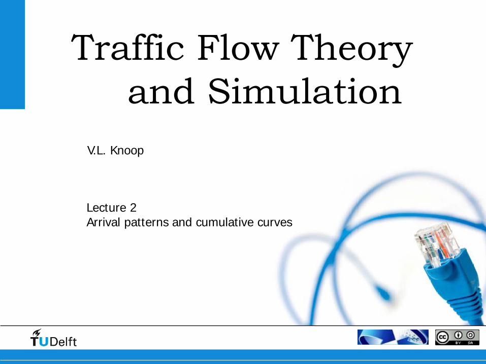
Excercise– a task for you!
• What is the average speed if you travel • 10 km/h from home to university• 20 km/h on the way back
• What is the average speed if you make a trip with speed• v1 on the outbound trip• v2 on the inbound trip
• What is the average speed if you split the trip in n equidistant sections, which you travel in vi

5Lecture 2 – Arrival patterns | 32
Similar problems arise in traffic
• Local measurements, spatial average speed needed
• Weigh speed measurements• Inversely proportional to speed
6Lecture 2 – Arrival patterns | 32
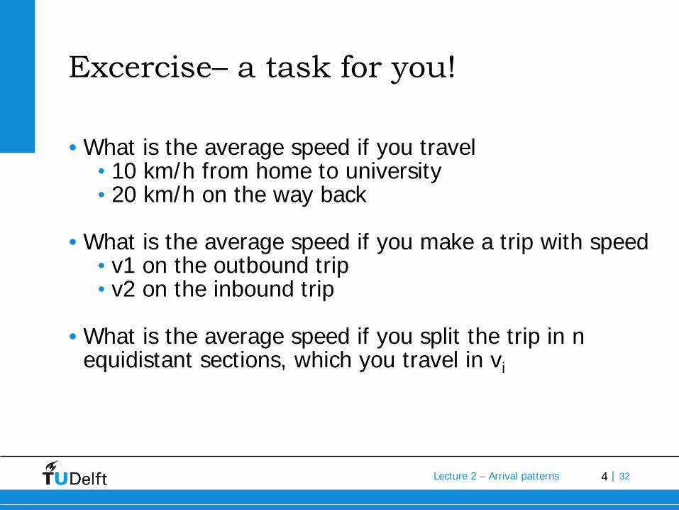
The math…
• Weigh speed measurements (w)• Inversely proportional to speed: wi=1/vi
Time-average of pace (1/v)
7Lecture 2 – Arrival patterns | 32
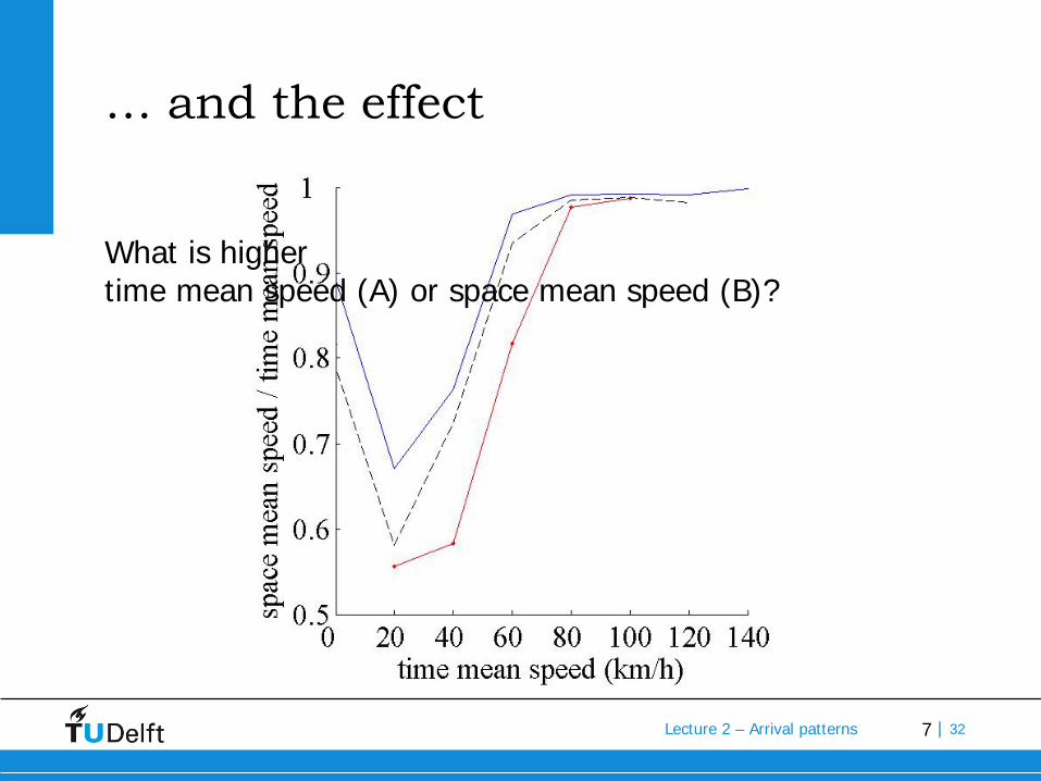
… and the effect
What is highertime mean speed (A) or space mean speed (B)?

8Lecture 2 – Arrival patterns | 32
Summary
• Speed averaging is not trivial
• Obtain time mean speed from loop detector data by harmonic average (i.e., averaging 1/v)
• Space mean speed is lower, with differences in practice up to factor 2
9Lecture 2 – Arrival patterns | 32
Overview of remainder of lecture
• Arrival process and relating probability distribution functions
• Poisson process (independent arrivals)• Neg. binomial distribution and binomial distribution• Applications facility design (determine length right-or left-turn lane)
• Time headway distributions• Distribution functions and headway models • Applications
• Speed distribution and free speed distributions
10Lecture 2 – Arrival patterns | 32
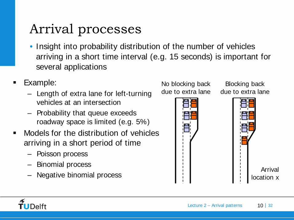
Arrival processes• Insight into probability distribution of the number of vehicles
arriving in a short time interval (e.g. 15 seconds) is important for several applications
No blocking backdue to extra lane
Blocking backdue to extra lane
Example:– Length of extra lane for left-turning
vehicles at an intersection– Probability that queue exceeds
roadway space is limited (e.g. 5%) Models for the distribution of vehicles
arriving in a short period of time– Poisson process– Binomial process– Negative binomial process
Arrivallocation x
11Lecture 2 – Arrival patterns | 32
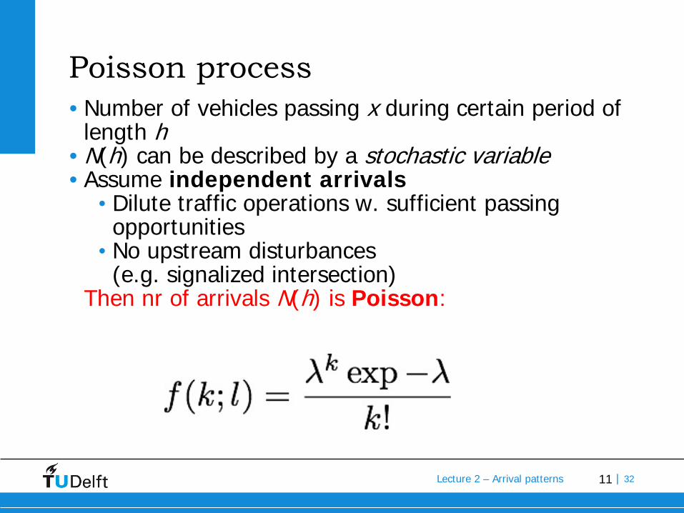
Poisson process• Number of vehicles passing x during certain period of
length h• N(h) can be described by a stochastic variable• Assume independent arrivals
• Dilute traffic operations w. sufficient passing opportunities
• No upstream disturbances (e.g. signalized intersection)
Then nr of arrivals N(h) is Poisson:
12Lecture 2 – Arrival patterns | 32
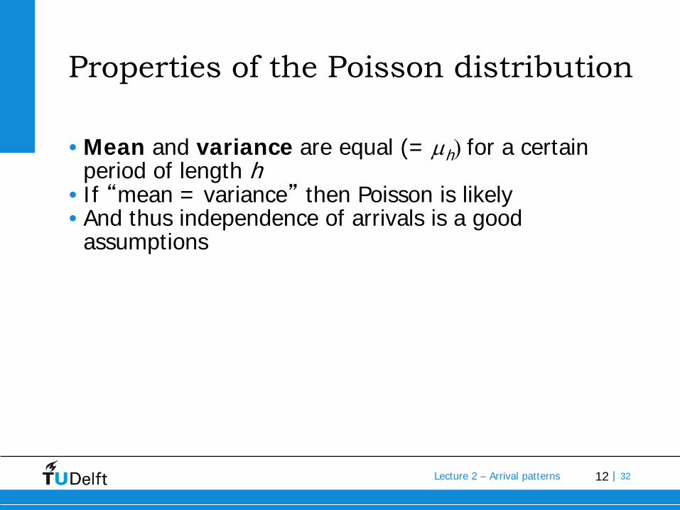
Properties of the Poisson distribution
• Mean and variance are equal (= µh) for a certain period of length h
• If “mean = variance” then Poisson is likely• And thus independence of arrivals is a good
assumptions
13Lecture 2 – Arrival patterns | 32
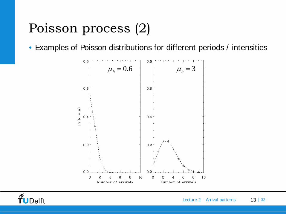
Poisson process (2)• Examples of Poisson distributions for different periods / intensities
3=hµ0.6=hµ

14Lecture 2 – Arrival patterns | 32
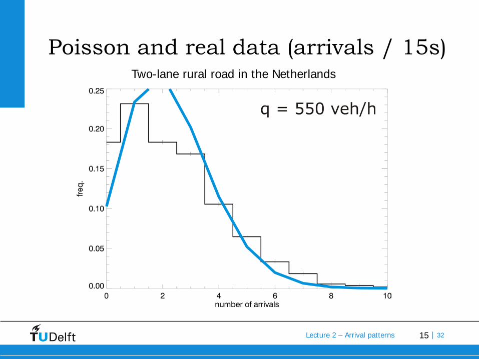
Poisson and real data (arrivals / 15s)Two-lane rural road in the Netherlands
15Lecture 2 – Arrival patterns | 32
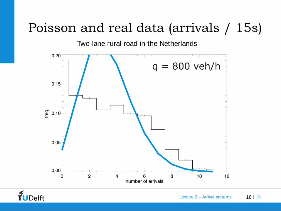
Poisson and real data (arrivals / 15s)Two-lane rural road in the Netherlands
16Lecture 2 – Arrival patterns | 32
Poisson and real data (arrivals / 15s)Two-lane rural road in the Netherlands
17Lecture 2 – Arrival patterns | 32
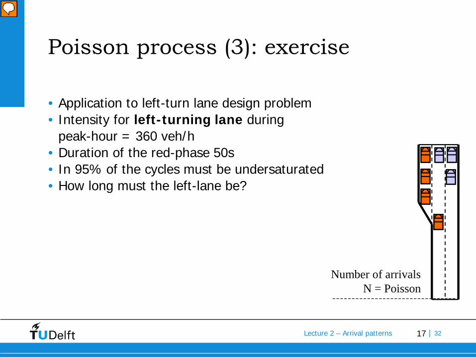
Poisson process (3): exercise
• Application to left-turn lane design problem• Intensity for left-turning lane during
peak-hour = 360 veh/h• Duration of the red-phase 50s• In 95% of the cycles must be undersaturated• How long must the left-lane be?
• Assume Poisson process; • Mean number of arrivals 50·(360/3600) = 5• Thus µh = 5 veh per ‘h’
(= qh with q = 360 and h = 50/3600) Number of arrivalsN = Poisson
18Lecture 2 – Arrival patterns | 32
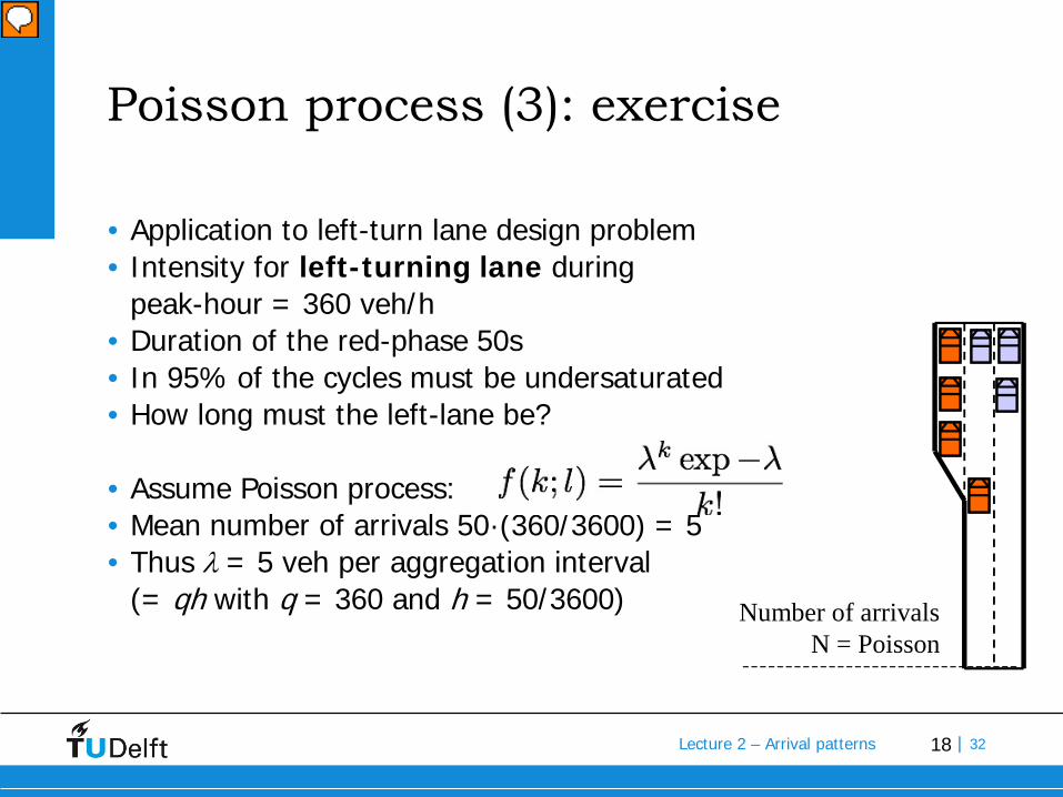
Poisson process (3): exercise
• Application to left-turn lane design problem• Intensity for left-turning lane during
peak-hour = 360 veh/h• Duration of the red-phase 50s• In 95% of the cycles must be undersaturated• How long must the left-lane be?
• Assume Poisson process:• Mean number of arrivals 50·(360/3600) = 5• Thus λ = 5 veh per aggregation interval
(= qh with q = 360 and h = 50/3600) Number of arrivalsN = Poisson

19Lecture 2 – Arrival patterns | 32
Poisson process (4)
• From graph:Pr(N≥8) = 0.9319Pr(N≥9) = 0.9682
• If the length of the left-turn lane can accommodate 9 vehicles, the probability of blocking back = 3.18%
20Lecture 2 – Arrival patterns | 32
Two other possibilities
1. Vehicles are (mainly) following=> binomial distribution
2. Downstream of a regulated intersection=> negative binomial distribtution

21Lecture 2 – Arrival patterns | 32
Binomial process
• Increase traffic flow yields formation of platoons (interaction)
• Poisson is no longer valid description• Alternative: Binomial process
• Binomial distribution describes the probability of nsuccessful, independent trials; the probability of success equals p; n0 = max. number of arrivals within period h
22Lecture 2 – Arrival patterns | 32
Properties of binomial distribution
• Mean: n0p and variance: n0(1 – p)p• Note that variance < mean• No rationale why approach yields reasonable results• Choose appropriate model by statistical testing!
23Lecture 2 – Arrival patterns | 32
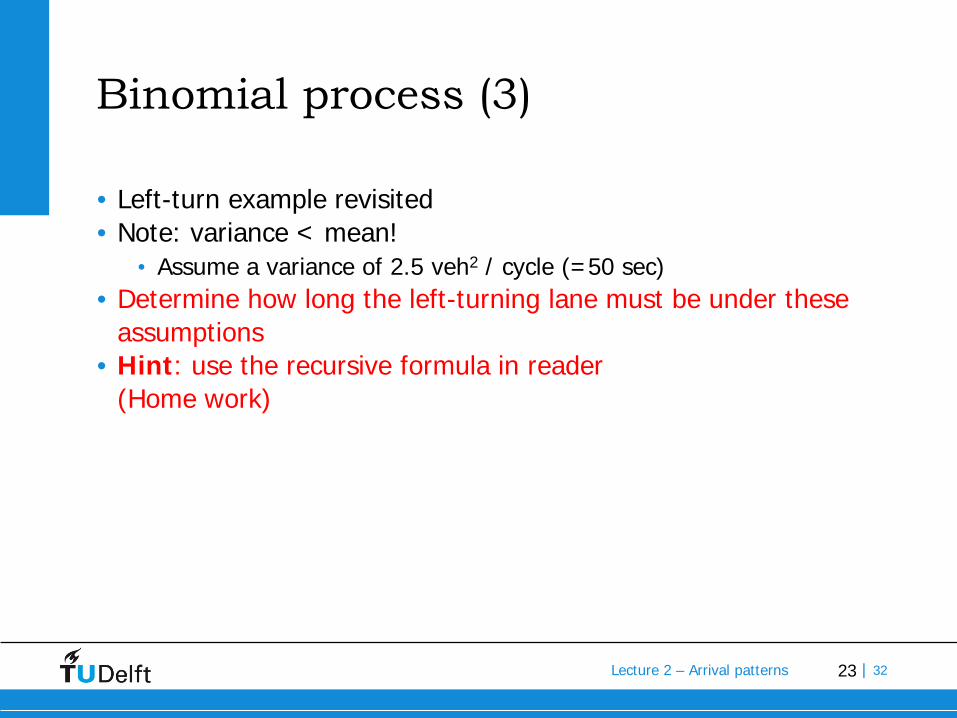
Binomial process (3)
• Left-turn example revisited• Note: variance < mean!
• Assume a variance of 2.5 veh2 / cycle (=50 sec)• Determine how long the left-turning lane must be under these
assumptions• Hint: use the recursive formula in reader
(Home work)
24Lecture 2 – Arrival patterns | 32
Downstream of controlled intersection
• More likely to have bunched vehicles(Why?)
• Negative binomial distribution

25Lecture 2 – Arrival patterns | 32
How to determine model to use?
Some guidelines:• Are arrivals independent => Poisson distribution
• Low traffic volumes• Consider traffic conditions upstream (but also downstream)
• Consider mean and variance of arrival process• Platooning due to regular increase in intensity?
=> Binomial• Downstream of signalized intersection?
=> Negative binomialDefinitive answer?• Use statistical tests (Chi-square tests) to figure out
which distribution is best
26Lecture 2 – Arrival patterns | 32
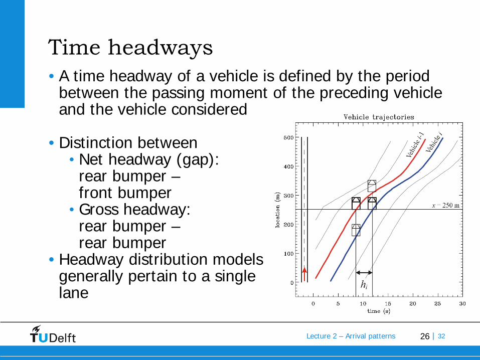
Time headways• A time headway of a vehicle is defined by the period
between the passing moment of the preceding vehicle and the vehicle considered
• Distinction between• Net headway (gap): rear bumper –front bumper
• Gross headway:rear bumper –rear bumper
• Headway distribution models generally pertain to a singlelane

27Lecture 2 – Arrival patterns | 32
Example headway distribution two-lane road
• Site: Doenkade
0 2 4 6 >8gross headway W (s)
0.0
0.2
0.4
0.6
0.8
hist
ogra
m

28Lecture 2 – Arrival patterns | 32
Exponential distribution
29Lecture 2 – Arrival patterns | 32
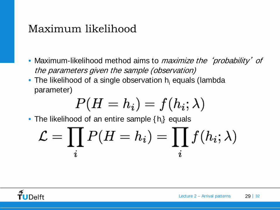
Maximum likelihood
• Maximum-likelihood method aims to maximize the ‘probability’ of the parameters given the sample (observation)
• The likelihood of a single observation hi equals (lambda parameter)
• The likelihood of an entire sample {hi} equals
30Lecture 2 – Arrival patterns | 32
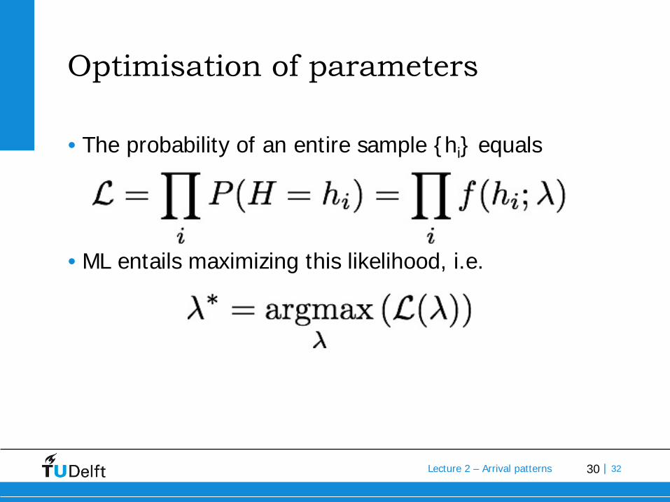
Optimisation of parameters
• The probability of an entire sample {hi} equals
• ML entails maximizing this likelihood, i.e.
31Lecture 2 – Arrival patterns | 32
Composite headway models
Composite headway models distinguish
• Vehicles that are driving freely (and thus arrive according to some Poisson process, or whose headways are exponentially distributed)
• Vehicles that are following at some minimum headway (so-called empty zone, or constrained headway)which distribution is suitable?

32Lecture 2 – Arrival patterns | 32
Basic idea
• Combine two distribution functionsContstraint: fraction phiFree: fraction (1-phi)
• Application: capactiy estimationHow?

33Lecture 2 – Arrival patterns | 32
Estimation: likelyhood or graphically

34Lecture 2 – Arrival patterns | 32
Summary
• Arrival distribution: Free flow: headways exponential,
nr of per aggregation time: PoissonFollowing: binomial
• Calculation of required dedicated lane length
• Composite headway models => capacity estimation
35Lecture 2 – Arrival patterns | 32
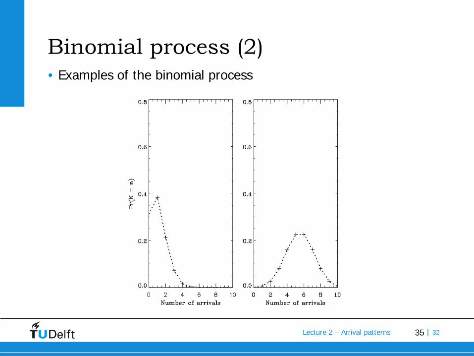
Binomial process (2)• Examples of the binomial process
36Lecture 2 – Arrival patterns | 32
Cowan’s M3 model
• Drivers have a certain minimum headway x which can be described by a deterministic variable
• Minimum headway x describes the headway a driver needs for safe and comfortable following the vehicle in front
• If a driver is not following, we assume that he / she is driving at a headway u which can be described by a random variate U ~ pfree(u)
• The headway h of a driver is the sum of the free headway u and the minimum headway x, and thus H = x+U
• The free headway is assumed distributed according to the exponential distribution (motivation?)
37Lecture 2 – Arrival patterns | 32
Cowan’s M3 model
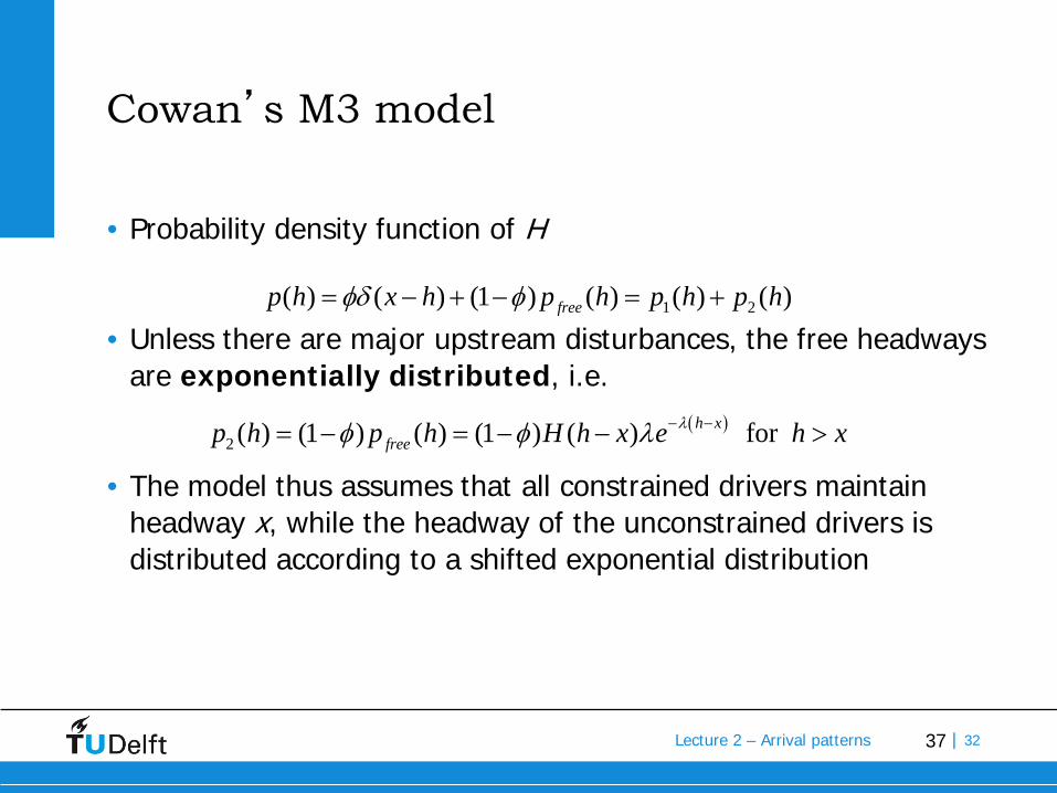
• Probability density function of H
• Unless there are major upstream disturbances, the free headways are exponentially distributed, i.e.
• The model thus assumes that all constrained drivers maintain headway x, while the headway of the unconstrained drivers is distributed according to a shifted exponential distribution
1 2( ) ( ) (1 ) ( ) ( ) ( )= − + − = +freep h x h p h p h p hφδ φ
( )2 ( ) (1 ) ( ) (1 ) ( ) for − −= − = − − >h x
freep h p h H h x e h xλφ φ λ

38Lecture 2 – Arrival patterns | 32
Cowan’s M3 model
• Example ofCowan’s M3 model
• (note that h0 = x)
39Lecture 2 – Arrival patterns | 32
Branston’s headway distribution model
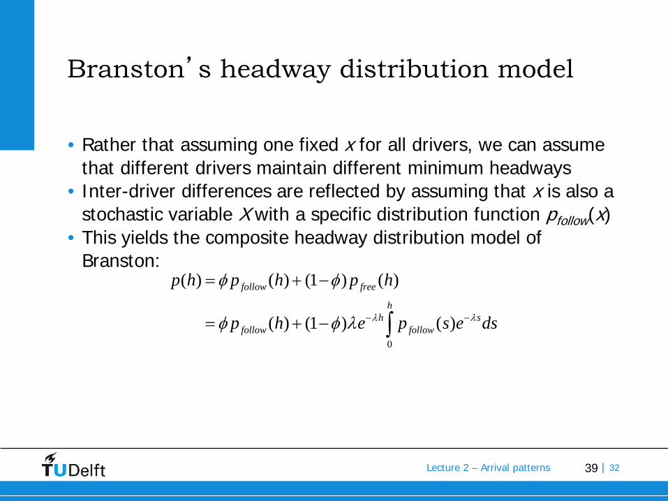
• Rather that assuming one fixed x for all drivers, we can assume that different drivers maintain different minimum headways
• Inter-driver differences are reflected by assuming that x is also a stochastic variable X with a specific distribution function pfollow(x)
• This yields the composite headway distribution model of Branston:
0
( ) ( ) (1 ) ( )
( ) (1 ) ( )− −
= + −
= + − ∫
follow free
hh s
follow follow
p h p h p h
p h e p s e dsλ λ
φ φ
φ φ λ

40Lecture 2 – Arrival patterns | 32
Buckley’s composite model
• Drivers have a certain minimum headway x which can be described by a random variable X ~ pfollow(x)
• Minimum headway describes the headway a driver needs for safe and comfortable following the vehicle in front
• X describes differences between drivers and within a single driver
• If a driver is not following, we assume that he / she is driving at a headway u which can be described by a random variate U ~ pfree(u)
• The headway h of a driver is then the minimum between the free headway u and the minimum headway x, and thus H = min{X,U}
41Lecture 2 – Arrival patterns | 32
Buckley’s composite model3
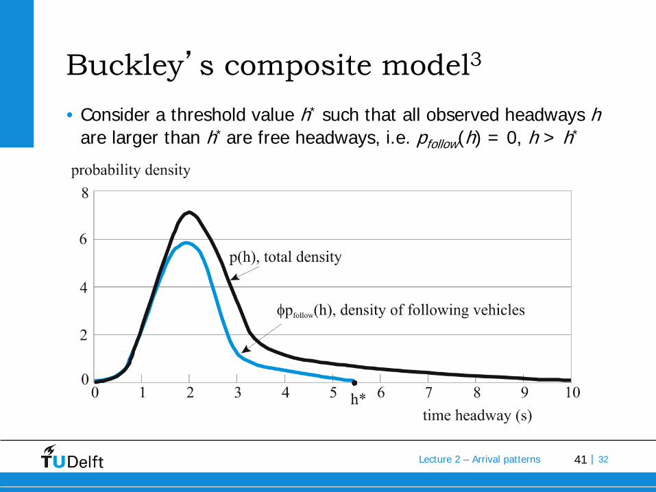
• Consider a threshold value h* such that all observed headways hare larger than h* are free headways, i.e. pfollow(h) = 0, h > h*
42Lecture 2 – Arrival patterns | 32
Buckley’s composite model4
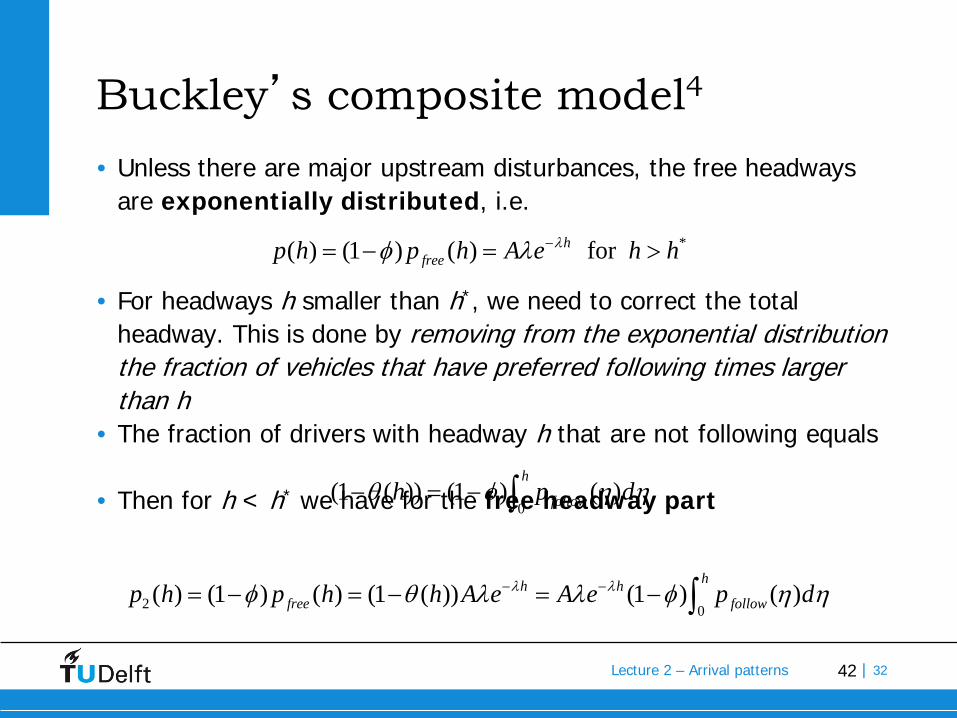
• Unless there are major upstream disturbances, the free headways are exponentially distributed, i.e.
• For headways h smaller than h*, we need to correct the total headway. This is done by removing from the exponential distribution the fraction of vehicles that have preferred following times larger than h
• The fraction of drivers with headway h that are not following equals
• Then for h < h* we have for the free headway part
*( ) (1 ) ( ) for hfreep h p h A e h hλφ λ −= − = >
0(1 ( )) (1 ) ( )
h
followh p dθ φ η η− = − ∫
2 0( ) (1 ) ( ) (1 ( )) (1 ) ( )
hh hfree followp h p h h A e A e p dλ λφ θ λ λ φ η η− −= − = − = − ∫

43Lecture 2 – Arrival patterns | 32
Buckley’s composite model5
• For the total headway distribution, we then get
where A denotes the normalization constant and can be determined from
• Special estimation procedures exist to determine λ, φ and p.d.f. pfollow(h)• Parametric: specify p.d.f. pfollow(h) with unknown parameters• Distribution free, non-parametric, i.e. without explicit specification pfollow(h)
0( ) ( ) (1 ) ( )
hhfollow followp h p h A e p dλφ φ λ η η−= + − ∫
0 0( ) 1 ( )followp d A e p dληη η λ η η
∞ ∞ −= ⇒ =∫ ∫

44Lecture 2 – Arrival patterns | 32
Determination of h*
• For h > h*, distribution is exponential, i.e.
• Consider survival function S(h)
• Obviously, for h > h*, we have • Suppose we have headway sample {hi}• Consider the empirical distribution function
• Now draw and determine h*, A, and λ
*( ) for hp h A e h hλλ −= >
( ) Pr( ) h
hS h H h A e d Aeλη λλ η
∞ − −= > = =∫
1ˆ ( ) 1 ( )n iS h H h hn
= − −∑
[ ]ln ( ) ln ln( )hS h Ae A hλ λ− = = −
ˆln ( )nS h
45Lecture 2 – Arrival patterns | 32
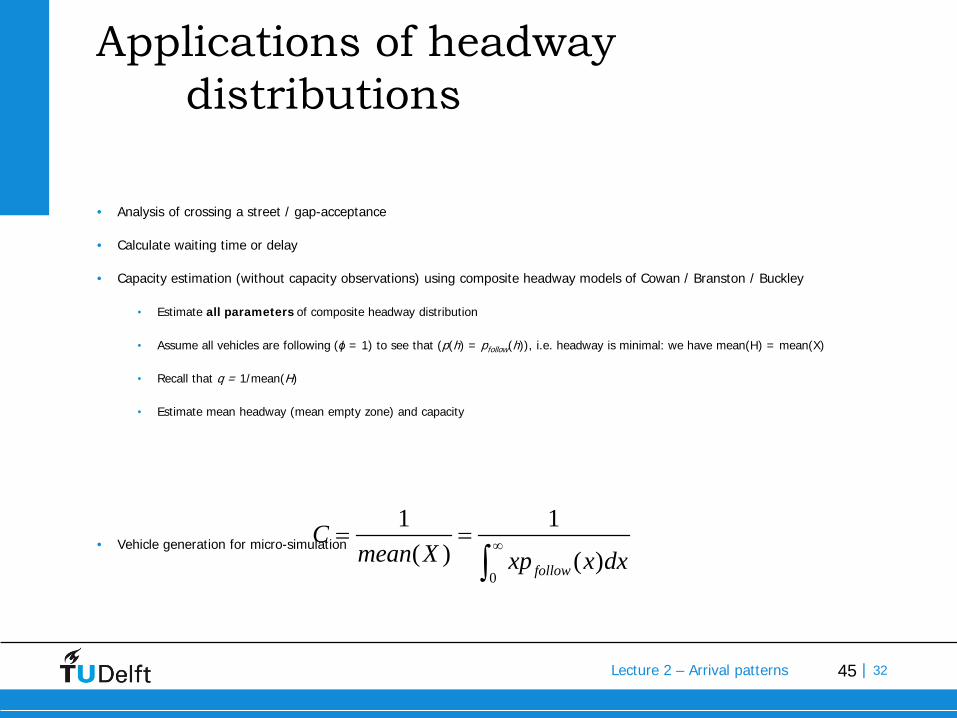
Applications of headway distributions
• Analysis of crossing a street / gap-acceptance
• Calculate waiting time or delay
• Capacity estimation (without capacity observations) using composite headway models of Cowan / Branston / Buckley
• Estimate all parameters of composite headway distribution
• Assume all vehicles are following (ϕ = 1) to see that (p(h) = pfollow(h)), i.e. headway is minimal: we have mean(H) = mean(X)
• Recall that q = 1/mean(H)
• Estimate mean headway (mean empty zone) and capacity
• Vehicle generation for micro-simulation
0
1 1( ) ( )follow
Cmean X xp x dx
∞= =∫
46Lecture 2 – Arrival patterns | 32
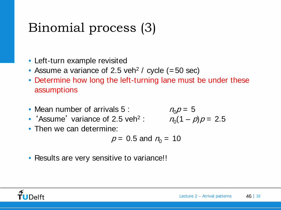
Binomial process (3)
• Left-turn example revisited• Assume a variance of 2.5 veh2 / cycle (=50 sec)• Determine how long the left-turning lane must be under these
assumptions
• Mean number of arrivals 5 : n0p = 5• ‘Assume’ variance of 2.5 veh2 : n0(1 – p)p = 2.5• Then we can determine:
p = 0.5 and n0 = 10
• Results are very sensitive to variance!!
47Lecture 2 – Arrival patterns | 32
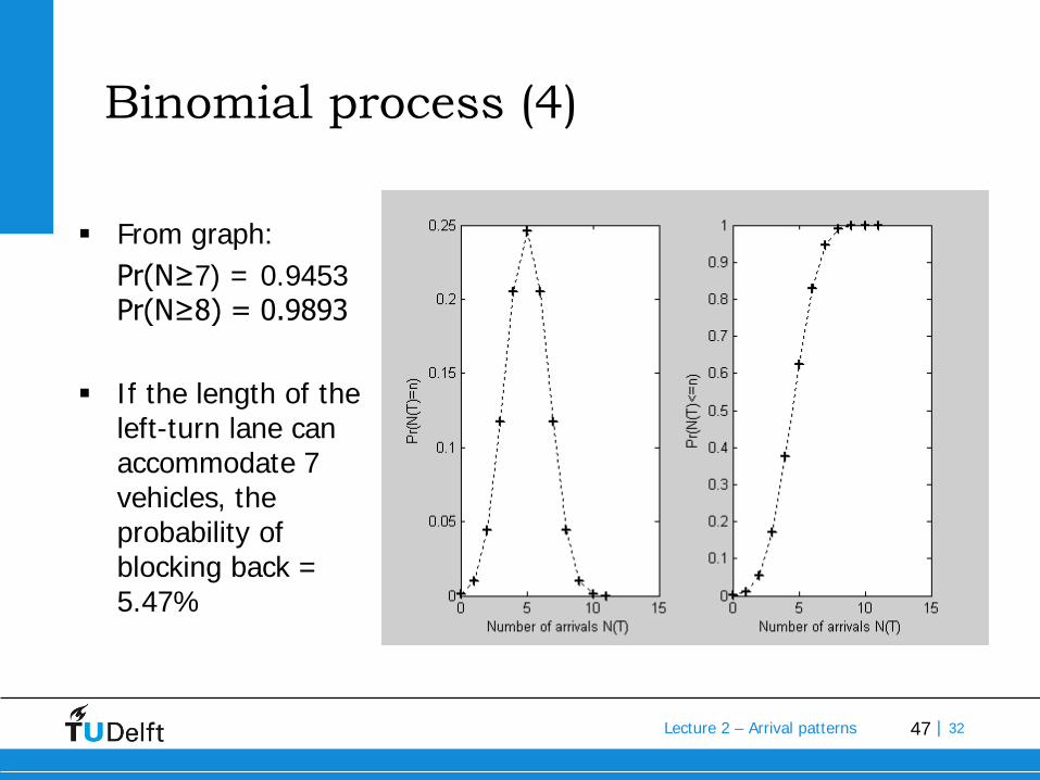
Binomial process (4)
From graph:Pr(N≥7) = 0.9453Pr(N≥8) = 0.9893
If the length of the left-turn lane can accommodate 7 vehicles, the probability of blocking back = 5.47%

48Lecture 2 – Arrival patterns | 32
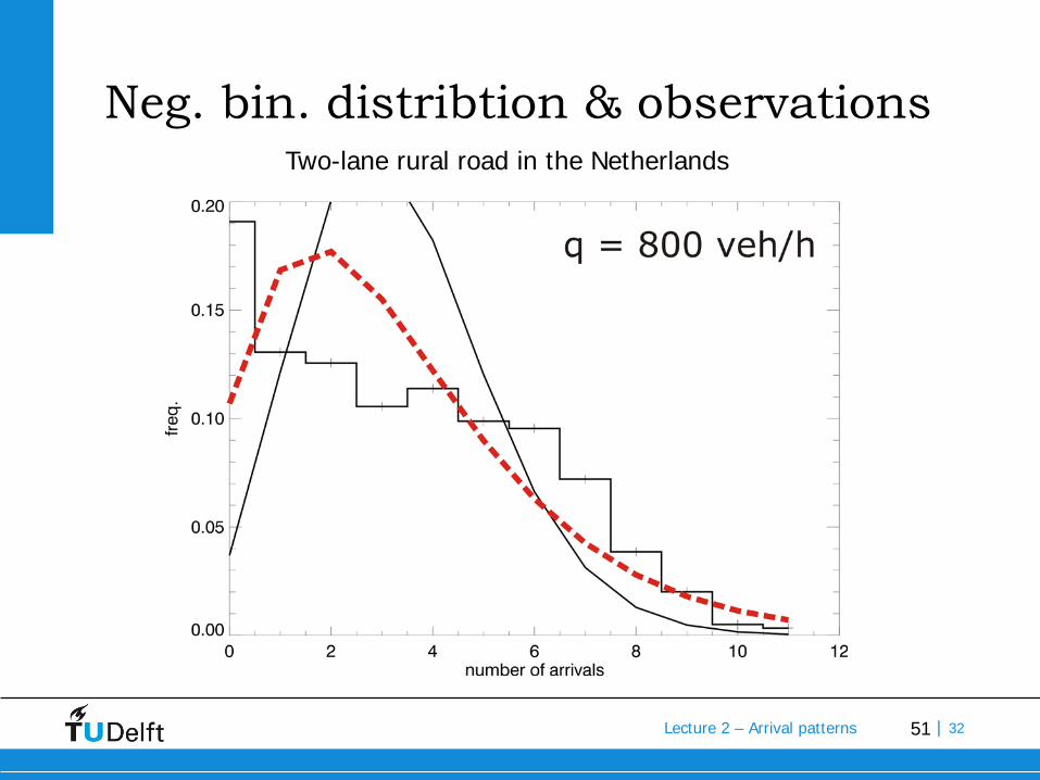
Negative Binomial distribution
• Also consider negative Binomial distribution (see course notes)
• Appears to hold when upstream disturbances are present
• Choose appropriate model by trial and error and statistical testing
( ) ( )00 1Pr ( ) 1 nnn n
N h n p pn
+ − = = −

49Lecture 2 – Arrival patterns | 32
Neg. bin. distribtion & observationsTwo-lane rural road in the Netherlands
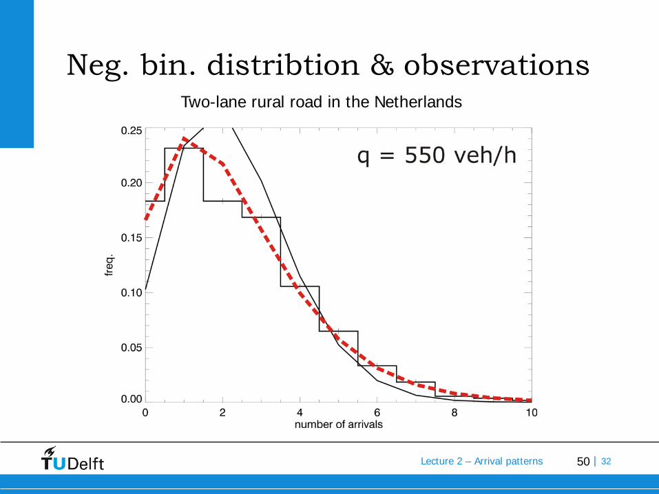
50Lecture 2 – Arrival patterns | 32
Neg. bin. distribtion & observationsTwo-lane rural road in the Netherlands
51Lecture 2 – Arrival patterns | 32
Neg. bin. distribtion & observationsTwo-lane rural road in the Netherlands
52Lecture 2 – Arrival patterns | 32
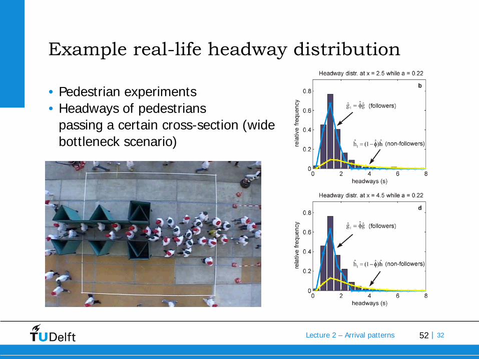
Example real-life headway distribution
• Pedestrian experiments• Headways of pedestrians
passing a certain cross-section (widebottleneck scenario)
53Lecture 2 – Arrival patterns | 32
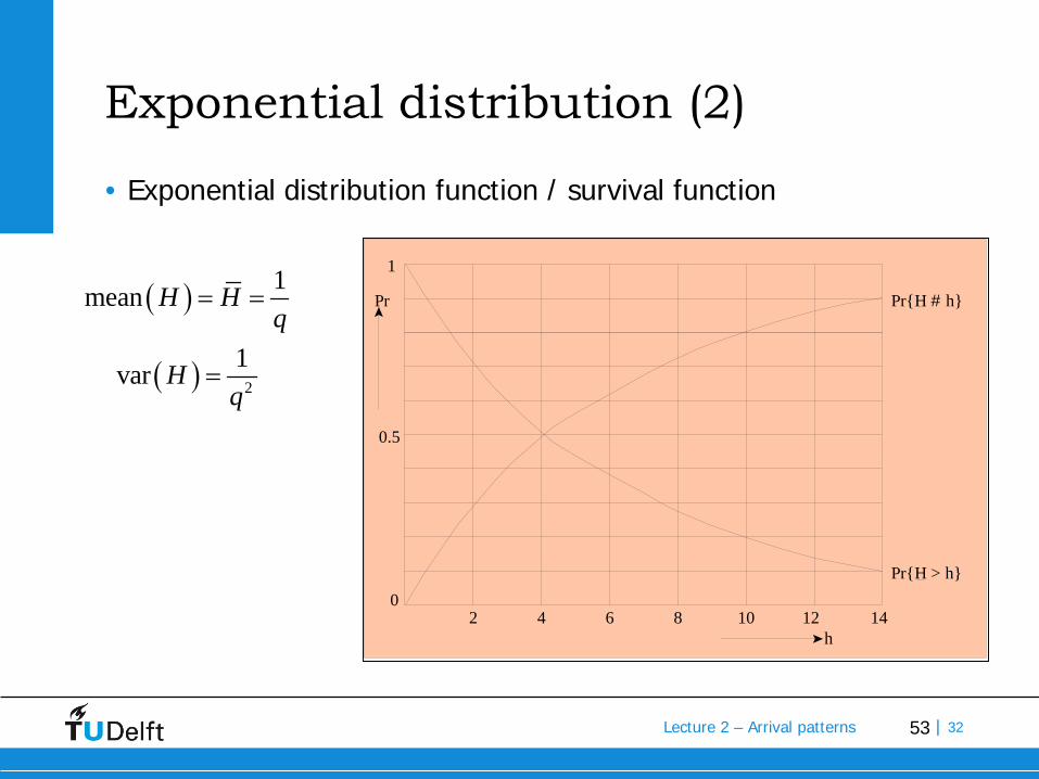
Exponential distribution (2)
• Exponential distribution function / survival function
1
0.5
Pr
0 2 4 6 8 10 12 14
h
Pr{H # h}
Pr{H > h}
( ) 1mean H Hq
= =
( ) 2
1var Hq
=

24-3-2014
Challenge the future
DelftUniversity ofTechnology
Cumulative curvesCalculation of delays and queues

55Lecture 2 – Arrival patterns | 32
Cumulative vehicle plots• Cumulative flow function Nx(t):
number of vehicles that have passed cross-section x at time instant t
• Nx(t): step function that increases with 1 each time instant vehicle passes
• Horizontal axis: trip times• Vertical axis: vehicle count
(storage)1( )xN t
2( )xN t
time (s)
time (s)

56Lecture 2 – Arrival patterns | 32
Examples of cumulative curves?
time
N 23
4
6
1
5
57Lecture 2 – Arrival patterns | 32
Construction of cumulative curves

58Lecture 2 – Arrival patterns | 32
Information in cumulative curves
time
N dN/dt = ??flow
59Lecture 2 – Arrival patterns | 32
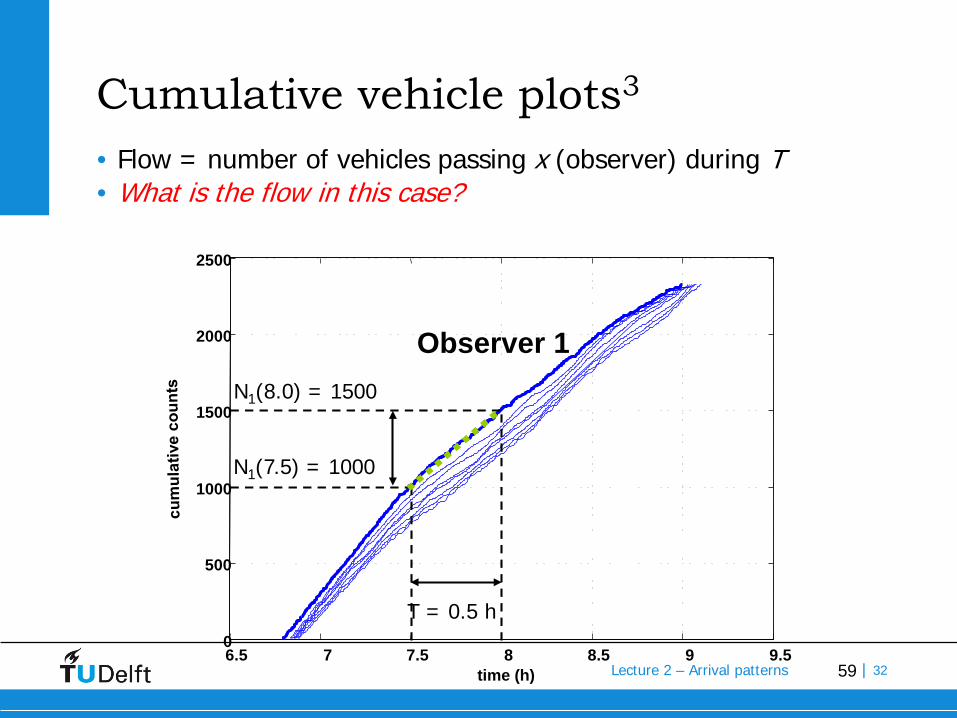
Cumulative vehicle plots3
• Flow = number of vehicles passing x (observer) during T• What is the flow in this case?
6.5 7 7.5 8 8.5 9 9.50
500
1000
1500
2000
2500
time (h)
Observer 1
T = 0.5 h
N1(7.5) = 1000
N1(8.0) = 1500
60Lecture 2 – Arrival patterns | 32
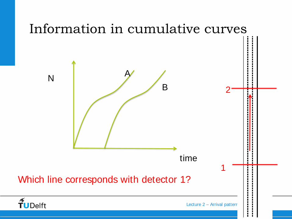
Information in cumulative curves
time1
2
Which line corresponds with detector 1?
N AB

61Lecture 2 – Arrival patterns | 32
62Lecture 2 – Arrival patterns | 32
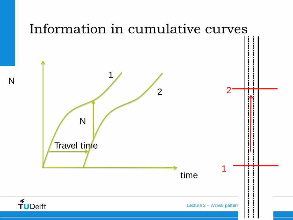
Information in cumulative curves
time
N
1
21
2
Travel time
N
63Lecture 2 – Arrival patterns | 32
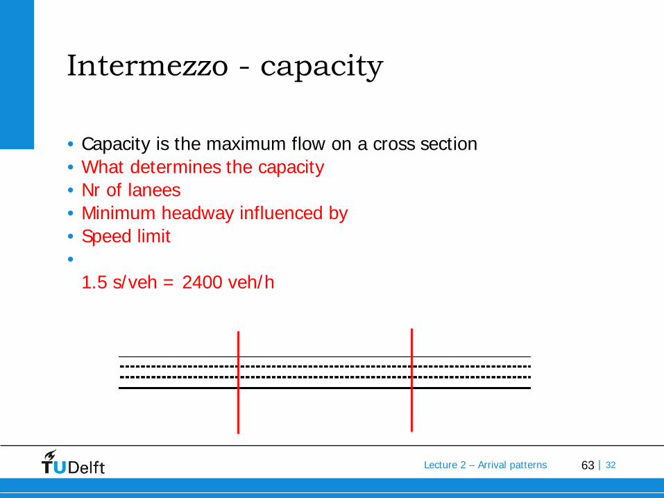
Intermezzo - capacity
• Capacity is the maximum flow on a cross section• What determines the capacity• Nr of lanees• Minimum headway influenced by• Speed limit•
1.5 s/veh = 2400 veh/h

64Lecture 2 – Arrival patterns | 32
Bottleneck in section

65Lecture 2 – Arrival patterns | 32
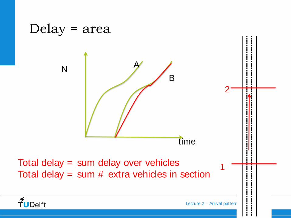
What if bottleneck is present
1
2
Flow limited to capacityTravel time incresesMore vehicles in the section
time
N AB
Travel time
66Lecture 2 – Arrival patterns | 32
Delay = area
time
1
2
Total delay = sum delay over vehiclesTotal delay = sum # extra vehicles in section
N AB

67Lecture 2 – Arrival patterns | 32
Controlled intersection

68Lecture 2 – Arrival patterns | 32
Delay (2)
Capacity
Capacity

69Lecture 2 – Arrival patterns | 32
Real-life curves
6.5 7 7.5 8 8.5 9 9.50
500
1000
1500
2000
2500
time (h)
cum
ulat
ive
coun
ts
Observer 1
Observer 8
Travel time vehicle 1000
Travel time vehicle 500
Number of vehicles between observer 1 and 8
Number of vehicles between observers can beused to determine density!
70Lecture 2 – Arrival patterns | 328.25 8.3 8.35 8.4 8.45 8.5 8.55 8.6 8.65 8.7 8.75
1600
1700
1800
1900
2000
2100
2200
time (h)
cum
ulat
ive
coun
ts
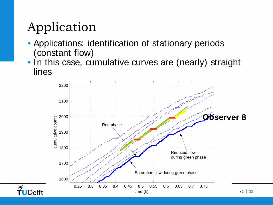
Saturation flow during green phase
Reduced flowduring green phase
Red phase
Application• Applications: identification of stationary periods
(constant flow)• In this case, cumulative curves are (nearly) straight
lines
Observer 8

71Lecture 2 – Arrival patterns | 32
Oblique curves• Amplify the features of the curves by applying an oblique scaling
rate q0• Use transformation: N2=N-q0t

72Lecture 2 – Arrival patterns | 32
Oblique curves
• Notice that density can still be determined directly from the graph; accumulation of vehicles becomes more pronounced
• This holds equally for stationary periods• For flows note that q0 needs to be added to the flow determined
from the graph by considering the slope op the slanted cumulative curve

73Lecture 2 – Arrival patterns | 32
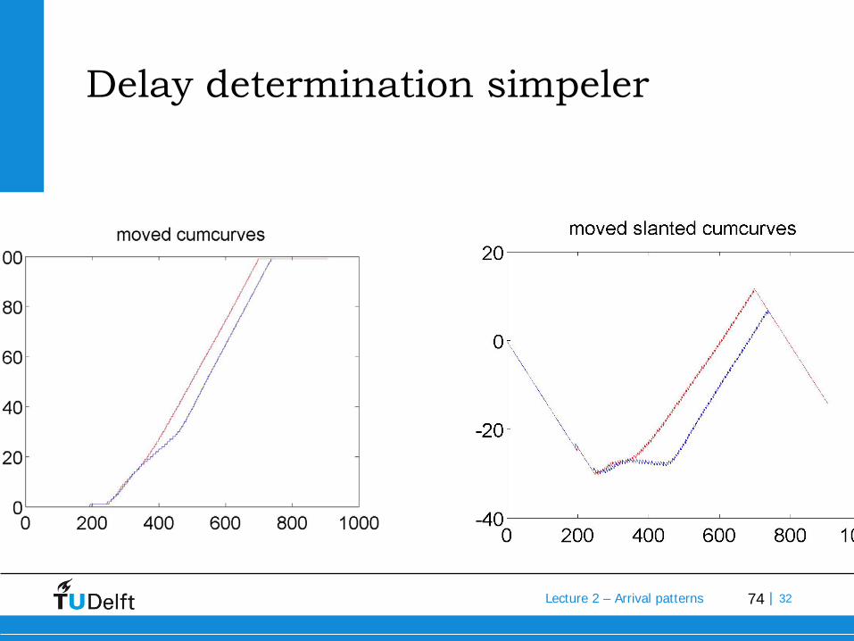
Use of oblique curves
• Can delay be read directly from oblique cumulative curvesA=yesB=no
• Can travel times be read directly from oblique cumulative curves?A=yesB=no
74Lecture 2 – Arrival patterns | 32
Delay determination simpeler

75Lecture 2 – Arrival patterns | 32
Deeper analysis
Capacity
Capacity
Demand
Capacity
Demand
Bottleneck

76Lecture 2 – Arrival patterns | 32
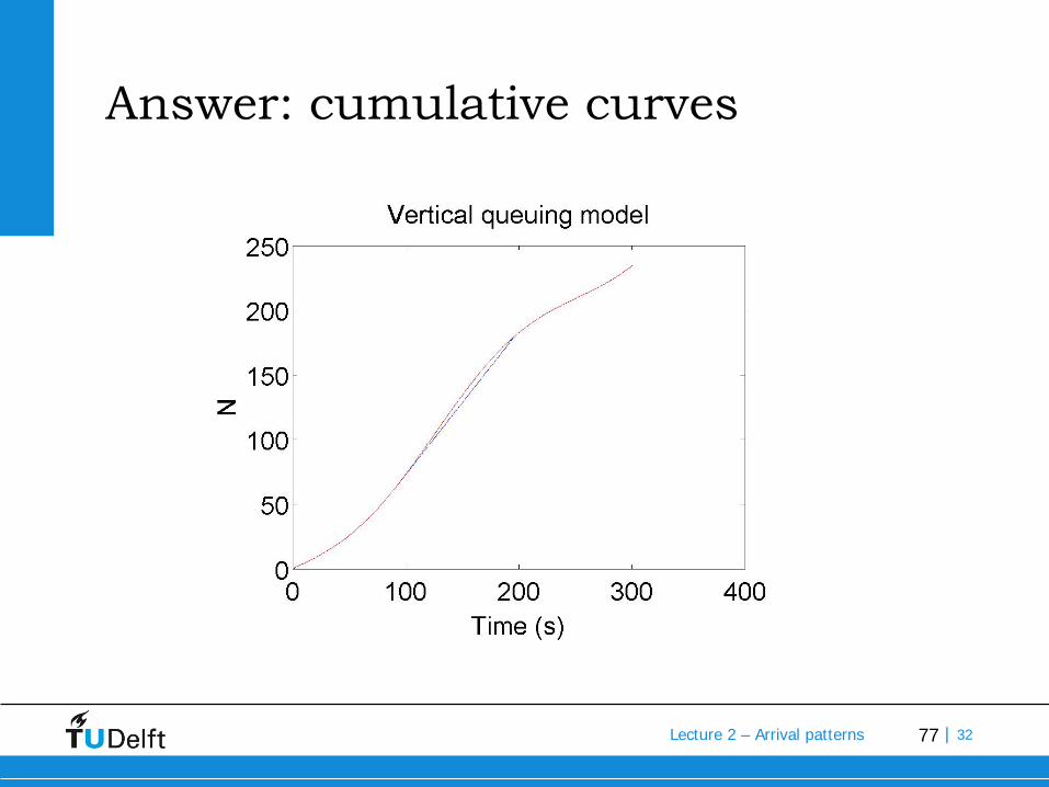
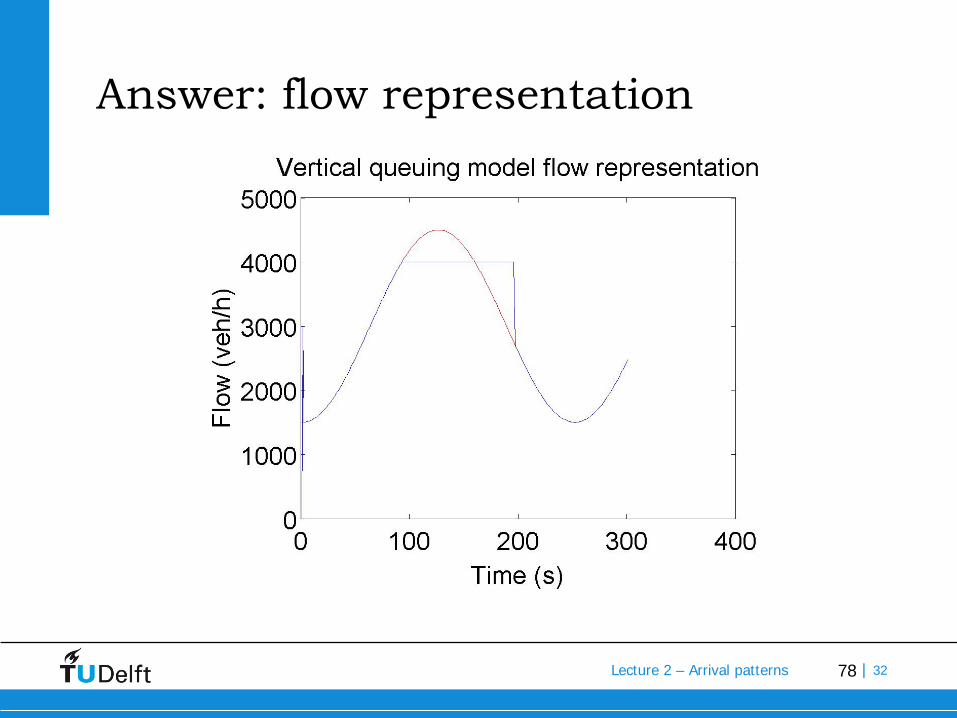
Simplest queuing model
• “Vertical queuing model”• Given the following demand profile, and capacity, give the
(translated) cumulative curves (and determine the delay)
77Lecture 2 – Arrival patterns | 32
Answer: cumulative curves
78Lecture 2 – Arrival patterns | 32
Answer: flow representation

79Lecture 2 – Arrival patterns | 32
Identifying capacity drop

80Lecture 2 – Arrival patterns | 32
Identifying capacity drop
• Using oblique (slanted) cumulative curves show that capacity before flow breakdown is larger than after breakdown (-300 veh/h)

81Lecture 2 – Arrival patterns | 32
Learning goals
• You now can:• Construct (slanted) fundamental diagrams• Use these to calculate:delays, travel times, density, flow
• In practice shortcoming:Data is corrupt, and errors accumulate
• Test yourself: tomorrow in excersise