Embed Size (px)
Citation preview

Viterbi School of Engineering Technology Transfer Center
A Statistical Physics Model of Technology Transfer
Ken DozierUSC Viterbi School of Engineering
Technology Transfer Center Technology Transfer Society (T2S)
26th Annual ConferenceAlbany, NY
October 1, 2004
Viterbi School of Engineering Technology Transfer Center
Presentation
• Problem (7 slides)
• Approach (9 slides)
• Results (5 slides)
• Conclusions (1 slide)
• Future (1 slide)
Viterbi School of Engineering Technology Transfer Center
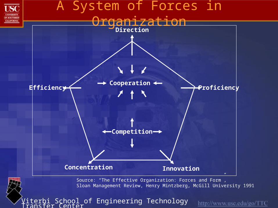
A System of Forces in Organization
Efficiency
Direction
Proficiency
Competition
Concentration Innovation
Cooperation
Source: “The Effective Organization: Forces and Form”,Sloan Management Review, Henry Mintzberg, McGill University 1991

Viterbi School of Engineering Technology Transfer Center
Make & Sell vs Sense & Respond
Chart Source:“Corporate Information Systems and Management”, Applegate, 2000
Viterbi School of Engineering Technology Transfer Center
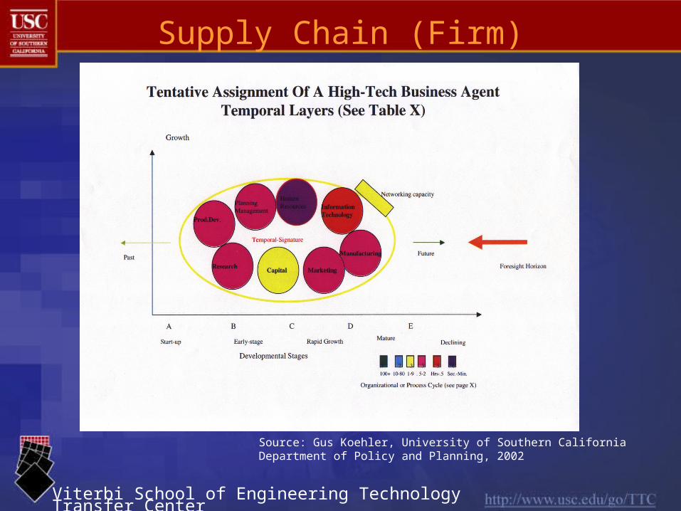
Supply Chain (Firm)
Source: Gus Koehler, University of Southern California Department of Policy and Planning, 2002

Viterbi School of Engineering Technology Transfer Center
Supply Chain (Government)
Source: Gus Koehler, University of Southern California Department of Policy and Planning, 2002
Viterbi School of Engineering Technology Transfer Center
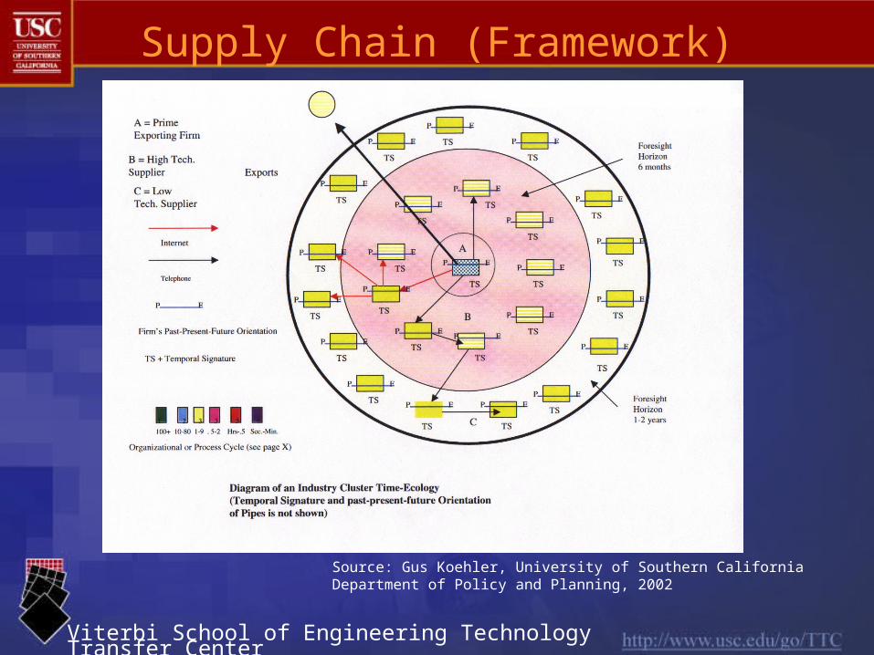
Supply Chain (Framework)
Source: Gus Koehler, University of Southern California Department of Policy and Planning, 2002
Viterbi School of Engineering Technology Transfer Center
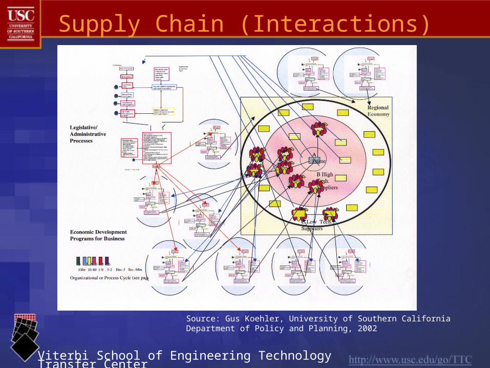
Supply Chain (Interactions)
Source: Gus Koehler, University of Southern California Department of Policy and Planning, 2002
Viterbi School of Engineering Technology Transfer Center
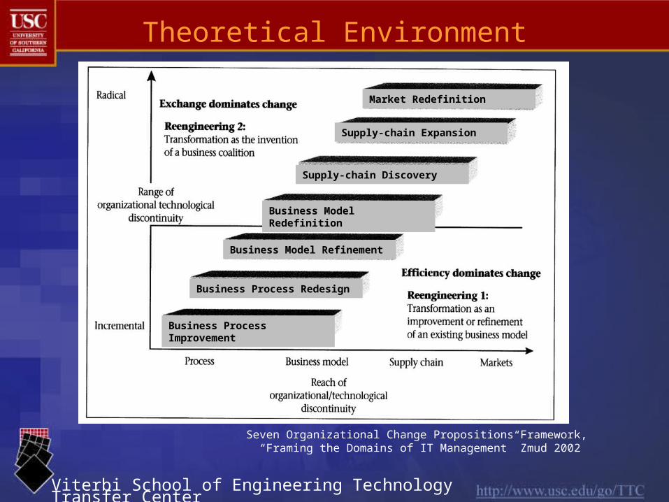
Theoretical Environment
Seven Organizational Change Propositions Framework, “Framing the Domains of IT Management” Zmud 2002
Business Process Improvement
Business Process Redesign
Business Model Refinement
Business Model Redefinition
Supply-chain Discovery
Supply-chain Expansion
Market Redefinition
Viterbi School of Engineering Technology Transfer Center
Framework Assumptions
• U.S. Manufacturing Industry Sectors can be Stratified using Average Company Size and Assigned to Layers of the Change Propositions
• Layers with Large Average Firm Size Will Have High B and Lowest T(1/B)
• Layers with Small Average Firm Size Will Have Low B and High T (1/B)
• The B and T Values Provide the Entry Point to Thermodynamics
Viterbi School of Engineering Technology Transfer Center
Thermodynamics ?
• Ample Examples of Support– Long Term Association with Economics
• Krugman, 2004
– Systems Far from Equilibrium can be Treated by (open systems) Thermodynamics
• Thorne, Fernando, Lenden, Silva, 2000
– Thermodynamics and Biology Drove New Growth Economics
• Costanza, Perrings, and Cleveland, 1997
– Economics and Thermodynamics are Constrained Optimization Problems
• Smith and Foley, 2002

Viterbi School of Engineering Technology Transfer Center
Thermodynamics ?
• Mathematical Complexity Could Discourage Practitioners
• Requires an Extension of Traditional Energy Abstractions
• Expansion May Require Knowledge to be Considered Pseudo Form of Energy?!
• Knowledge Potential and Kinetic States?!– Patent: potential
– Technology Transfer: Kinetic
– Tacit versus Explicit

Viterbi School of Engineering Technology Transfer Center
• Thermodynamics
– A systematic mathematical technique for determining what can be inferred from a minimum amount of data
• Key: Many microstates possible to give an observed macrostate
• Basic principle: Most likely situation given by maximization of the number of microstates consistent with an observed macrostate
• Why “pseudo’?
– Conventional thermodynamics: “energy” rules supreme– Thermodynamics of economics phenomena: “energy” shown
by statistical physics analysis to be replaced by quantities related to “productivity, i.e. output per employee”
Constrained Optimization Approach
Viterbi School of Engineering Technology Transfer Center
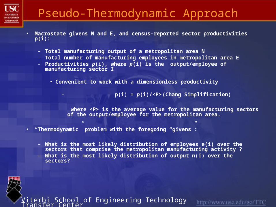
Pseudo-Thermodynamic Approach
• Macrostate givens N and E, and census-reported sector productivities p(i):
– Total manufacturing output of a metropolitan area N– Total number of manufacturing employees in metropolitan area E– Productivities p(i), where p(i) is the output/employee of manufacturing
sector I
• Convenient to work with a dimensionless productivity
– p(i) = p(i)/<P> (Chang Simplification)
where <P> is the average value for the manufacturing sectors of the output/employee for the metropolitan area.
• “Thermodynamic” problem with the foregoing “givens”:
– What is the most likely distribution of employees e(i) over the sectors that comprise the metropolitan manufacturing activity ?
– What is the most likely distribution of output n(i) over the sectors?
Viterbi School of Engineering Technology Transfer Center
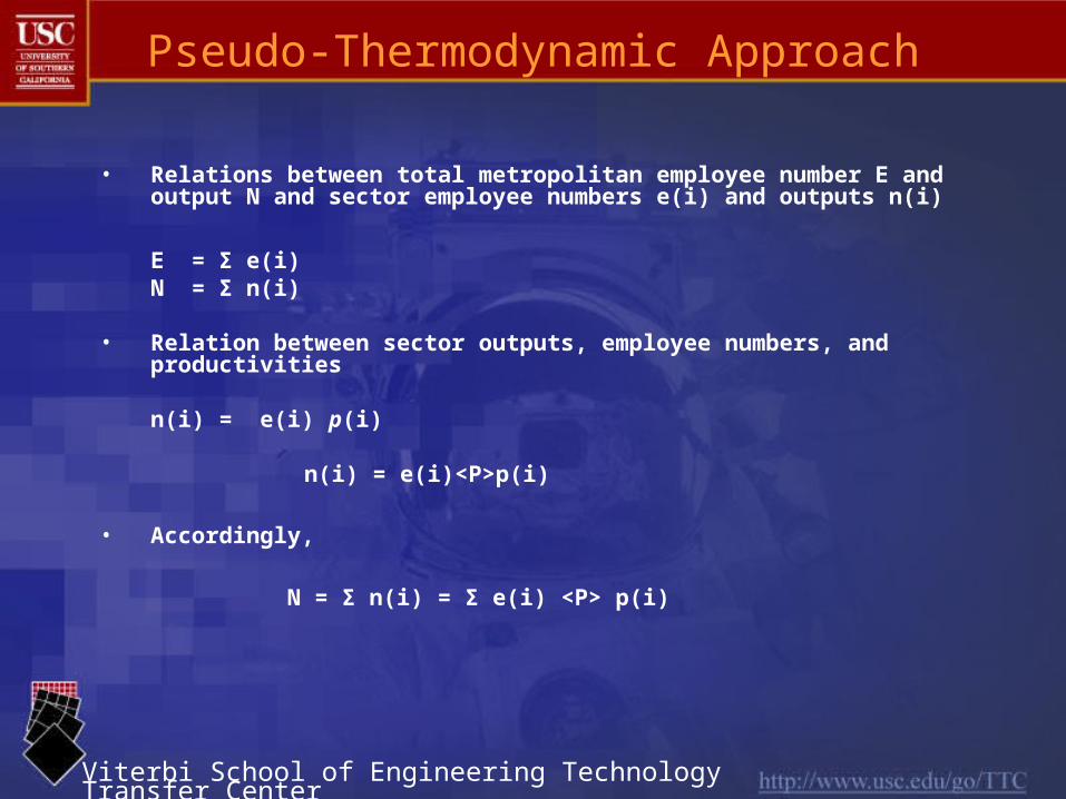
• Relations between total metropolitan employee number E and output N and sector employee numbers e(i) and outputs n(i)
E = Σ e(i)
N = Σ n(i)
• Relation between sector outputs, employee numbers, and productivities
n(i) = e(i) p(i)
n(i) = e(i)<P>p(i)
• Accordingly,
N = Σ n(i) = Σ e(i) <P> p(i)
Pseudo-Thermodynamic Approach

Viterbi School of Engineering Technology Transfer Center
• Look for the (microstate) distribution e(i) that will give the maximum number of ways W in which a known (macrostate) N and E can be achieved.
– Number of ways (distinguishable permutations) in which N and E can be achieved
W = [N! / ∏ n(i)!][E! / ∏ e(i)!]
• Maximization of W subject to constraint equations of previous slide
– Introduce Lagrange multipliers and β to take into account constraint equations
– Deal with lnW rather than W in order to use Stirling approximation for natural logarithm of factorials for large numbers
ln{n!} => n ln{n}- n when n >>1
Pseudo-Thermodynamic Approach
Viterbi School of Engineering Technology Transfer Center
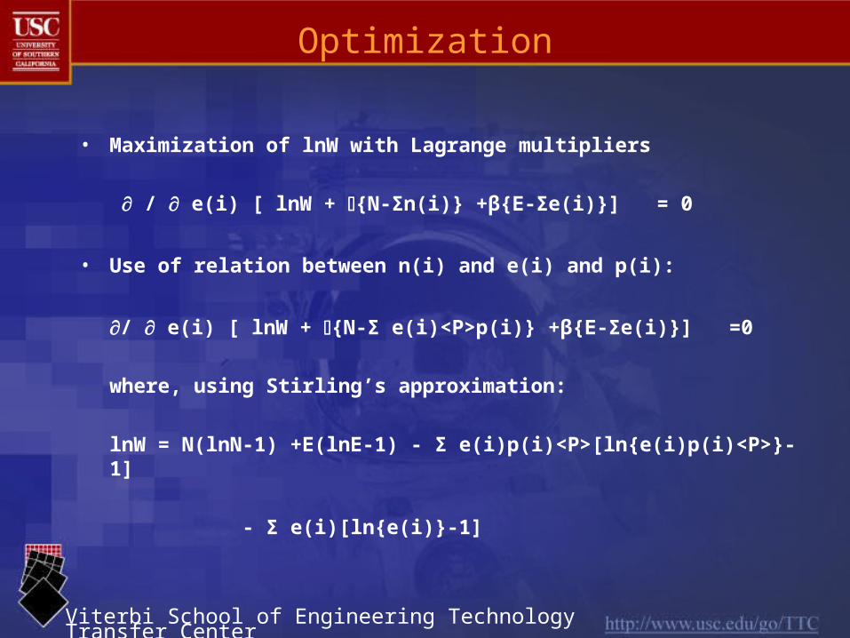
• Maximization of lnW with Lagrange multipliers
/ e(i) [ lnW + {N-Σn(i)} +β{E-Σe(i)}] = 0
• Use of relation between n(i) and e(i) and p(i):
/ e(i) [ lnW + {N-Σ e(i)<P>p(i)} +β{E-Σe(i)}] =0
where, using Stirling’s approximation:
lnW = N(lnN-1) +E(lnE-1) - Σ e(i)p(i)<P>[ln{e(i)p(i)<P>}-1]
- Σ e(i)[ln{e(i)}-1]
Optimization
Viterbi School of Engineering Technology Transfer Center
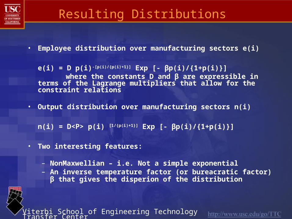
• Employee distribution over manufacturing sectors e(i)
e(i) = D p(i)-[p(i)/{p(i)+1}] Exp [- βp(i)/{1+p(i)}]
where the constants D and β are expressible in terms of the Lagrange multipliers that allow for the constraint relations
• Output distribution over manufacturing sectors n(i)
n(i) = D<P> p(i) [1/{p(i)+1}] Exp [- βp(i)/{1+p(i)}]
• Two interesting features:
– NonMaxwellian – i.e. Not a simple exponential– An inverse temperature factor (or bureacratic factor) β that
gives the disperion of the distribution
Resulting Distributions

Viterbi School of Engineering Technology Transfer Center
Figure 1: Predicted shape of output n(i) vs. productivity p(i) for a sector bureaucratic factor β = 0.1 [lower curve] and β=1 [upper curve].
n(i)
p(i)
Output

Viterbi School of Engineering Technology Transfer Center
Figure 2. Predicted shape of employee number e(i) vs. productivity p(i) for a sector bureaucratic factor β = 0.1 [lower curve] and β=1 [upper curve].
e(i)
p(i)
Employment
Viterbi School of Engineering Technology Transfer Center
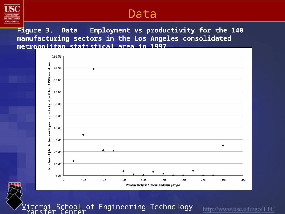
Figure 3. Data Employment vs productivity for the 140 manufacturing sectors in the Los Angeles consolidated metropolitan statistical area in 1997
0.00
10.00
20.00
30.00
40.00
50.00
60.00
70.00
80.00
90.00
100.00
0 100 200 300 400 500 600 700 800 900
Productivity in $ thousands/employee
Nu
mb
er o
f jo
bs
in t
ho
usa
nd
s p
er p
rod
uct
ivit
y b
in w
idth
s o
f $5
0K/e
mp
loye
e
Data
Viterbi School of Engineering Technology Transfer Center
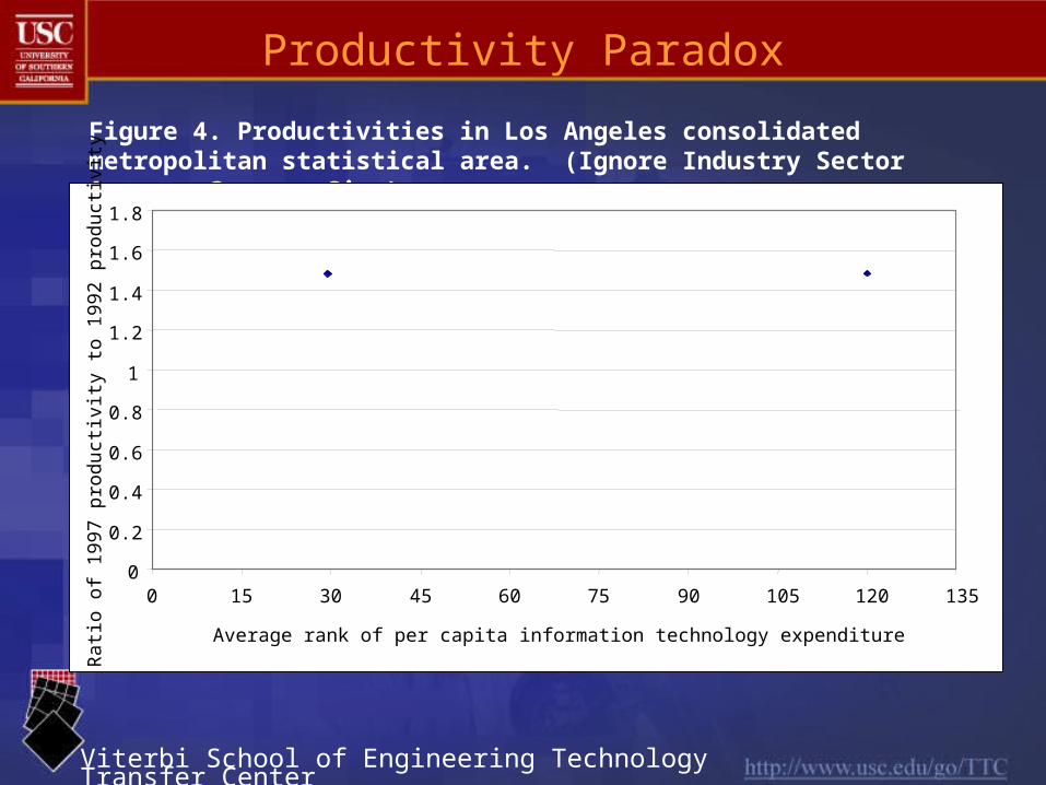
Productivity Paradox
Figure 4. Productivities in Los Angeles consolidated metropolitan statistical area. (Ignore Industry Sector Average Company Size)
0
0.2
0.4
0.6
0.8
1
1.2
1.4
1.6
1.8
0 15 30 45 60 75 90 105 120 135
Average rank of per capita information technology expenditure
Rat
io o
f 199
7 pr
oduc
tivity
to 1
992
prod
uctiv
ity
Viterbi School of Engineering Technology Transfer Center
0
0.2
0.4
0.6
0.8
1
1.2
1.4
1.6
1.8
0 15 30 45 60 75 90 105 120 135
Average rank of per capita information technology expenditure
Rat
io o
f 199
7 pr
oduc
tivity
to 1
992
prod
uctiv
ity
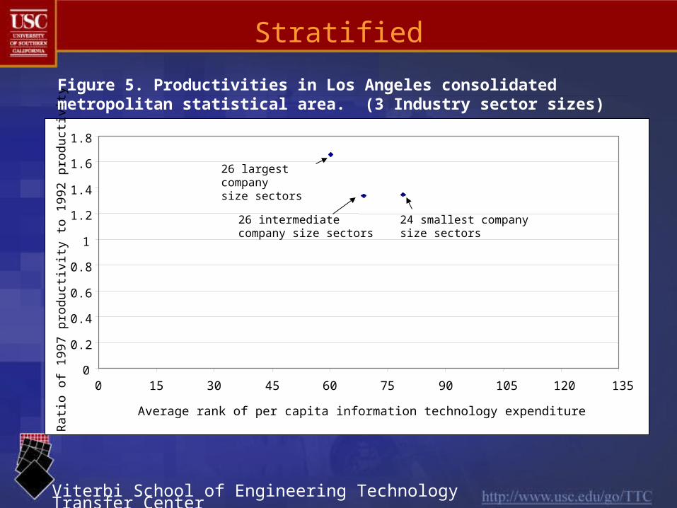
Stratified
Figure 5. Productivities in Los Angeles consolidated metropolitan statistical area. (3 Industry sector sizes)
26 largest company size sectors
26 intermediate company size sectors
24 smallest company size sectors
Viterbi School of Engineering Technology Transfer Center
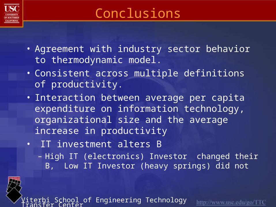
Conclusions
• Agreement with industry sector behavior to thermodynamic model.
• Consistent across multiple definitions of productivity.
• Interaction between average per capita expenditure on information technology, organizational size and the average increase in productivity
• IT investment alters B– High IT (electronics) Investor changed their B, Low IT
Investor (heavy springs) did not
Viterbi School of Engineering Technology Transfer Center
Future Work
• Examine NAICS consistent 2002 and 1997 U.S. manufacturing economic census data
• Use seven organizational change proposition strata to further explore the linkage between organizational size and productivity.
• Compare results across the strata and within each stratum
• Check for compliance to thermodynamic model
• Expand to technology transfer

Viterbi School of Engineering Technology Transfer Center
Variable Physics Economics
State (i) Hamiltonian eigenfunction Production site
Energy Hamiltonian eigenvalue Ei Unit production cost Ci
Occupation number Number in state Ni Production output Ni
Partition function Z ∑exp[-(1/kBT)Ei] ∑exp[-βCi]
Free energy F kBT lnZ (1/β) lnZ
Generalized force fξ ∂F/∂ξ ∂F/∂ξ
Example Pressure TechnologyExample Electric field x charge Knowledge
Entropy (randomness) - ∂F / ∂T kBβ2∂F/∂ξ
Comparison of Statistical Formalism in Physics and in Economics
Viterbi School of Engineering Technology Transfer Center
0.5 1 1.5 2
1
2
3
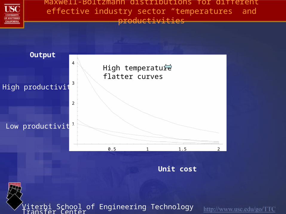
4High temperature flatter curves
High productivity
Low productivity
Output
Unit cost
Maxwell-Boltzmann distributions for different effective industry sector “temperatures” and productivities
Viterbi School of Engineering Technology Transfer Center
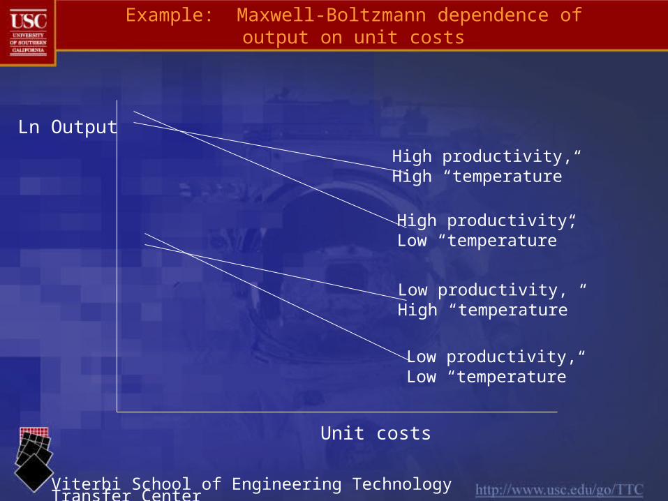
Ln Output
Unit costs
High productivity,High “temperature”
High productivity,Low “temperature”
Low productivity,High “temperature”
Low productivity,Low “temperature”
Example: Maxwell-Boltzmann dependence of output on unit costs
Viterbi School of Engineering Technology Transfer Center
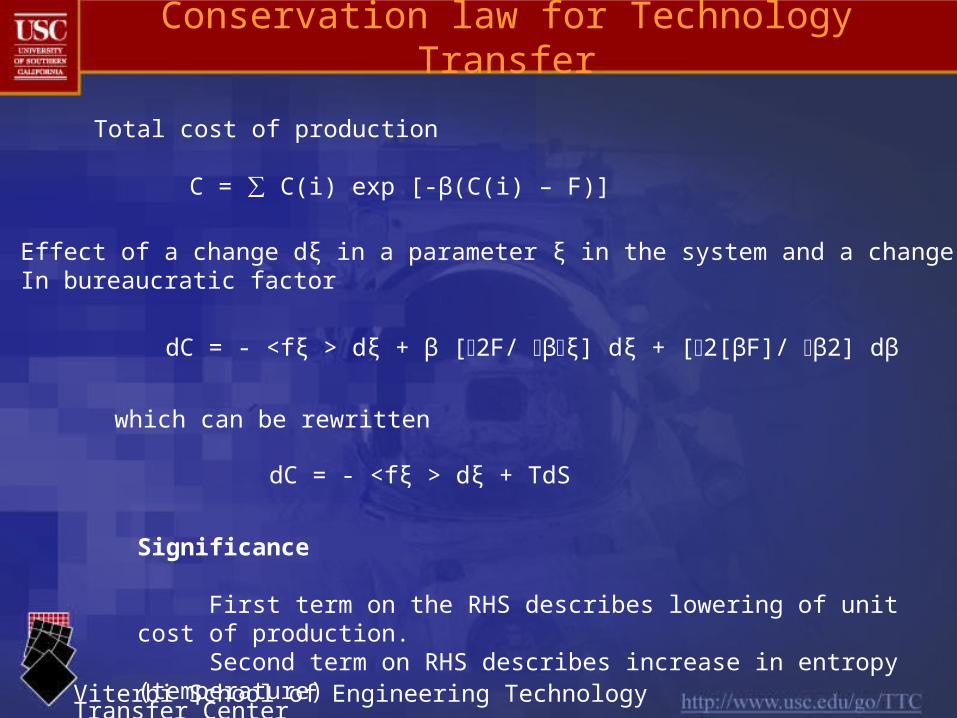
Total cost of production
C = ∑ C(i) exp [-β(C(i) – F)]
Effect of a change dξ in a parameter ξ in the system and a change d βIn bureaucratic factor
dC = - <fξ > dξ + β [2F/ βξ] dξ + [2[βF]/ β2] dβ
which can be rewritten
dC = - <fξ > dξ + TdS
Significance First term on the RHS describes lowering of unit cost of production. Second term on RHS describes increase in entropy (temperature)
Conservation law for Technology Transfer

Viterbi School of Engineering Technology Transfer Center
Ln Output
Unit costs
High productivity,High “temperature”
High productivity,Low “temperature”
Low productivity,High “temperature”
Low productivity,Low “temperature”
Costs down
Entropy up
Effects of Technology Transfer
Viterbi School of Engineering Technology Transfer Center
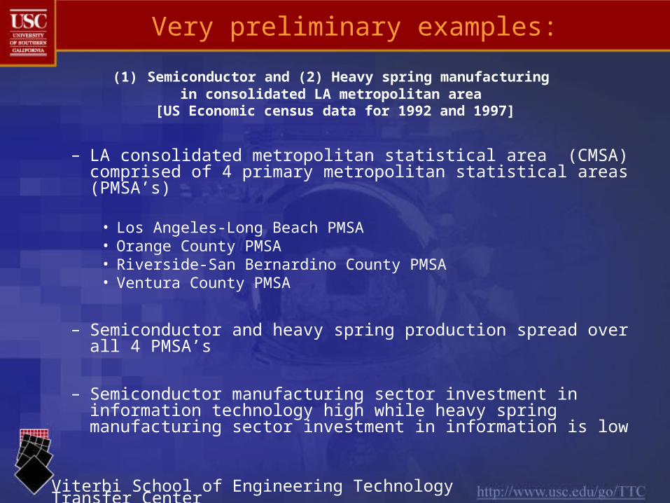
(1) Semiconductor and (2) Heavy spring manufacturing in consolidated LA metropolitan area
[US Economic census data for 1992 and 1997]
– LA consolidated metropolitan statistical area (CMSA) comprised of 4 primary metropolitan statistical areas (PMSA’s)
• Los Angeles-Long Beach PMSA• Orange County PMSA• Riverside-San Bernardino County PMSA• Ventura County PMSA
– Semiconductor and heavy spring production spread over all 4 PMSA’s
– Semiconductor manufacturing sector investment in information technology high while heavy spring manufacturing sector investment in information is low
Very preliminary examples:

Viterbi School of Engineering Technology Transfer Center
• Observations on a sector with large investment in information
– Correlation between PMSA’s with highest production and lowest unit costs
• Qualitatively consistent with a Boltzmann distribution
– Large decrease in temperature (increase in bureaucratic factor) between 1992 and 1997
• slope 7 x larger in 1997 than in 1992
– Large increase in employee productivity between 1992 and 1997 • Value of shipments per employee 1.8 x larger in 1997
[$230K/employee] than in 1992
Example 1. Semiconductor production in consolidated LA metropolitan area in 1992 and 1987

Viterbi School of Engineering Technology Transfer Center
Ln Output
Unit costs
High productivity,High “temperature”
High productivity,Low “temperature”
Low productivity,High “temperature”
Low productivity,Low “temperature”
Semiconductor example: Movement between 1992 and 1997 on Maxwell Boltzmann plot
Viterbi School of Engineering Technology Transfer Center
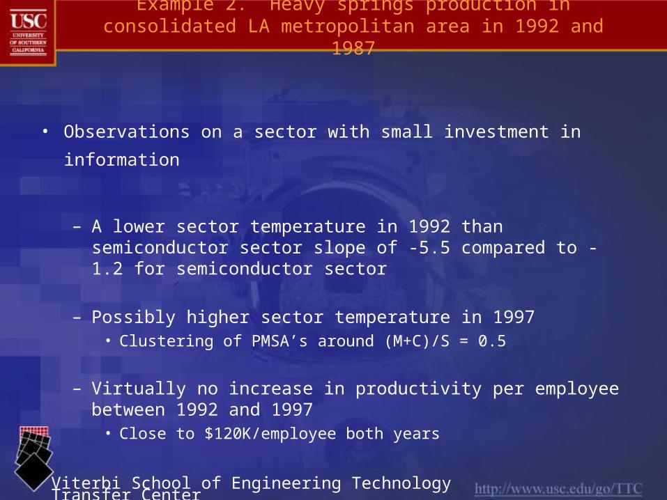
• Observations on a sector with small investment in information
– A lower sector temperature in 1992 than semiconductor sector slope of -5.5 compared to -1.2 for semiconductor sector
– Possibly higher sector temperature in 1997• Clustering of PMSA’s around (M+C)/S = 0.5
– Virtually no increase in productivity per employee between 1992 and 1997
• Close to $120K/employee both years
Example 2. Heavy springs production in consolidated LA metropolitan area in 1992 and 1987
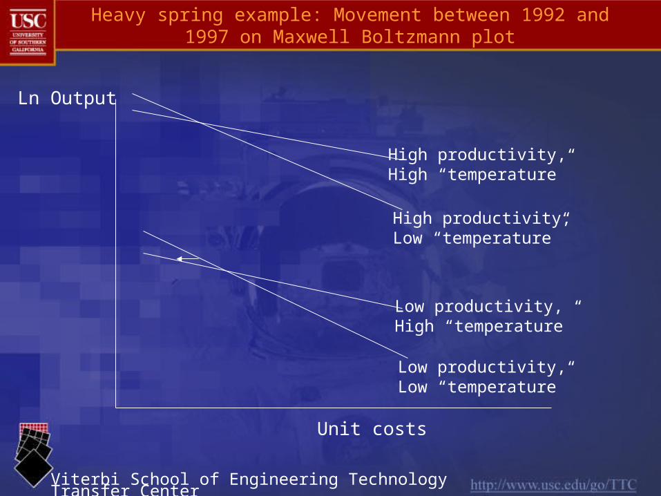
Viterbi School of Engineering Technology Transfer Center
Ln Output
Unit costs
High productivity,High “temperature”
High productivity,Low “temperature”
Low productivity,High “temperature”
Low productivity,Low “temperature”
Heavy spring example: Movement between 1992 and 1997 on Maxwell Boltzmann plot