Visualization of Scalar Topology for Structural

Visualization of Scalar Topology for Structural Enhancement

C. L. Bajaj V. Pascucci Department of Computer Sciences and TICAM

University of Texas, Austin, TX 78733 D. R. Schikore

Center for Applied Scientific Computing Lawrence Livermore National Laboratory, Livermore, CA 945 50

Abstract

Scalar fields arise in every scientific application. Existing scalar visualization techniques require that the user infer the global scalar structure from what is frequently an insufficient display of information. We present a visualization technique which nu- merically detects the structure at all scales, removing from the user the responsibility of extracting information implicit in the data, and presenting the structure explicitly for analysis. We further demonstrate how scalar topology detection proves useful for correct visualization and image processing applications such as image co-registxation, isocontouring, and mesh com- pression.

Keywords: Scientific Visualization, Scalar Fields, Curves and Surfaces, Vector Topology

1 Introduction

Visualization of scalar fields is common across all scientific dis- ciplines, including geographic data such as altitude and temper- ature, medical applications with CT and MRI values, and pres- sure and vorticity magniinde in computational fluid dynamics. The purpose of the visualization is to aid the user in understand- ing the structure of the ditta[29].

Common methods for visualizing scalar fields can be grouped into two broad classes. First are methods whose aim is to detect smicture and present a display to the user which communicates this structure. Critical to these methods is the definition of structure:, and how well the definition matches the visualization users’ need. Second are those methods which attempt to display the entire scalar field simultaneously, leav- ing interpretation of the display to the user. Combinations of the two methods serve to reinforce the information provided by each visualization. We aril1 use for comparison one technique from each of these categories, isocontouring and colormapping.

Isocontours, or constant valued curves and surfaces from continuous 2D and 3D s d a r fields, are a common visualization technique for displaying scalar field structure[2 11. By their definition, isocontours represent the data only at discrete lev- els, and as such are an ef€ective technique for determining the

“shape” of objects in the scalar field. Shape extraction as defined by isocontours is well understood and appreciated in many applications, such as Medical Imaging, as isocontours in a den- sityfield may result in realistic models of skeletal structure, skin surface, or various organs[22]. Also implicit in their definition is the fact that isocontours are an incomplete representation of the scalar field, as one can only infer from an isocontour that the data to one side is above the isovalue, and the data to the other side is below the isovalue. With multiple isocontours, the scalar field effectively becomes segmented into a finite number of ranges, within which the structure remains unknown. The same claim of incompleteness can be made of any technique which only displays a portion of the field. Moreover it is not obvious which isovalues one should select and how namy of them [4].

Colormapping of scalar data defines a discrete or continuous range of colors onto which the scalar values are mapped. Use of color, though proven to be useful in many visualization techniques, introduces complications due of perceptual issues, such as colorblindness. Colormaps may also mislead the user, for example when small-scale structure in the data is washed out due to the large range of values taken on by the variable.

Scientific data which is time-varying in nature intensifies the problems with the methods described above. In the typical case, a scalar variable may take on a wide range of values over the course of a simulation, however at certain times during the simulation the range may be much smaller. With both isocontours and colormapped display, it is desirable to use the same isovalues and colormap for each time-step being displayed in order to reduce the possibility of introducing artifacts which may be misinterpreted as features. This requirement complicates the task of choosing a good colormap or selection of isovalues for a time-varying visualization.

In this paper we present a complementary scalar structure visualization technique which does not depend on the user to determine structure from the graphical display, but instead defines, computes, and displays the structure of a scalar field di- rectly. Through detection of all critical points (saddles, m a - ima, and minima), we construct an embedded graph by computing integral curves in the gradient field fiom saddle points to an attached critical point, as illustrated in figure 1. Curves in

0-8 186-9176-x/98/$10.00 Copyright 1998 IEEE

51

Figure 1: Isocontours (dotted) ofpart of a scalar field along with the critical points and integral curves

this topological graph are always perpendicular to isocontours ofthe scalar field[23], and we will demonstrate that these curves contain complementary information to that provided by display of isocontours or colormapped scalar fields, providing a method which is both useful in its own right and which also enhances the commonly used techniques for visualizing scalar fields. We further indicate that the definition of structure which is provided by the scalar topology proves useful in several additional visualization and image processing applications.

2 Related Work Much of the work in enhancing colormapped visualization of scalar fields has dealt with determining “good” colormaps which effectively display the data. Bergman, et. al., define rules based on perception, user goals, and data characteristics to automatically select a colormap which will meet the user requirements[6]. Histogram equalization is a technique which spreads the data evenly over the range of colors, using the available color space to it’s fullest[28]. The result is that each color in the colormap is used an equal number of times. Gershon[ 141 uses “Generalized Animation” to display otherwise static scalar data in a dynamic way, taking advantage of the ability of the visual system to detect dynamic changes. Animation draws at- tention to fuzzy details in the data which may not be detected in the static representation.

There has been several papers in detecting isocontours in 2d and 3d scalar data[2l, 301. Additional work concentrates on handling problems in regions containing saddle points which cause difficulty in determining the topological structure of the surface contained in the region [25,3 1,261. The problem ofde- tecting ridges and valleys in digital terrain has been treated in several papers[ 121. McCormack, et. al. consider the problem of detecting drainage pattems in geographic terrain[24]. Inter- rante, et. al. have used ridge and valley detection on 3d surfaces to enhance the shape of transparently rendered surfaces[ 191. Extrema graphs were used by Itoh and Koyamada to speed isocontour extraction[20]. A graph containing extreme points and boundary points of a scalar field can be guaranteed to intersect

every isocontour at least once, allowing seed points to be gener- ated by searching only the cells contained in the extrema graph.

Helman and Hesselink detect vector field topology by clas- sifying the zeros of a vector field and performing particle tracing from saddle points[ 171. The resulting partitioning consists of regions which are topologically equivalent to uniform flow. Globus, et. al. describe a software system for 3d vector topology and briefly note that the technique may also be applied to the gradient of a scalar field in order to identify maxima and minima[ 151. Bader et. al. and Collard et. al. examine the gradient field of the charge density in a molecular system[2, 1, lo]. The topology of this scalar field represents the bonds linking to- gether the atoms of the molecule. Bader goes on to show how features higher level structures in the topologyrepresent chains, rings, an cages in the molecule. Bader’s example is a defin- ing motivation for developing the automatic extraction and visualization of topology from a scalar field. In many situations, topology provides a more intuitive and physically meaningful visualization. Grosse [ 161 also presents methods of approxi- mating the scalar topology of the electron density function of proteins. One of his methods uses tensor product B-spline fits while the other scales Fourier coefficients of the electron density function.

3 Scalar Topology Previous techniques for enhancing scalar field visualization attempt to address the inability of colormapping and isocontouring to capture and directlyrepresent features in the data. We address this problem not through feature enhancement using existing visualization techniques, but through direct feature detection and display. For our purpose of detection and display, we define the topology of a scalar field S defined with domain D to consist of the following:

1. The local maxima of S

2. The local minima of S

3. The saddle points of S

4. Selected integral curves joining each of the above

Integral curves are defined as curves which are everywhere tangent to the gradient field of S. Intuitively, these curves represent the path followed by a heat-seeking particle in a temper- ature field, or the path followed by a ball rolling down a hill in a field of elevation values. In vector field topology, the curves ad- vected in the flow field segment the field into regions which are topologically equivalent to uniform flow. In the case of scalar topology, integral curves segment the field into regions in which the gradient flow is uniform, or in other words, the scalar function is monotonic. Such a segmentation>of the scalar field into regions of simple behavior reveals the structure of the scalar field for the visualization user.

We outline the procedure for visualization of scalar topology as follows:

52

1. Detect stationary (critical) points in S.

2. Classify stationary points.

3. Integrate selected integral curves in gradient field.

In the following subsections, we will define our model of a continuous scalar field and look at each of the steps defined above.

3.1 Scalar Field Model

In typical scientific applications, data is represented at the nodes of a mesh of elements and interpolated linearly across the interior of the elements. Such a data model is CO continuous and has a discontinuous gradient field, making it unsuitable for our purpose of tracing integral curves in the gradient field. We seek to construct a data model such that:

1. The original nodal <data is interpolated.

2. The gradient at the boundaries is CO continuous.

3. Critical points in the scalar field are not removed, and the number introduced is kept small.

i

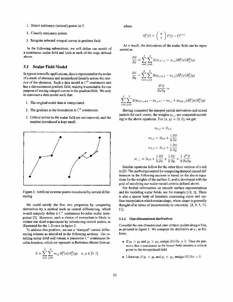
I Figure 2: Artificial extreme points introduced by central differencing

We could satisfy the first two properties by computing derivatives by a method such as central differencing, which would uniquely define a C1 continuous bi-cubic scalar interpolant [3]. However, such a choice of interpolant is likely to violate our third requirement by introducing critical points, as illustrated for the I-D case in figure 2.

To address this problem, we use a “damped” central differencing scheme as described in the following sections. The resulting scalar field will n:main a piecewise C1 continuous bicubic function, which we :represent in Bernstein-B6zier form as:

where

As a result, the derivatives of the scalar field can be represented as:

-- - d2S dxdy

n n

Having computed the damped partial derivatives and mixed partials for each vertex, the weights w i j are computed accord- ing to the above equations. For (x, y) = (0,O) , we get:

w0,o = s 0 , o

W 0 , l = s 0 , o + -- 1 dS 3 a x 1 a s

w1,o = s0,o + -- 3 dY

1as 1dS 1 d2S W 1 , l = S0,O + -- + -- + -- 3 a x 3 a y g a x a y

Similar equations follow for the other three vertices of a cell in2D. The method presented for computing damped central differences in the following sections is based on the above equations for the weights of the surface S, and is developed with the goal of satisfying our scalar model criteria defined above.

For fbrther information on smooth surface representations and for modeling scalar fields, see for example [ 18, 31. There is also a sparse body of literature concerning curve and surface interpolation which retains shape, where shape is generally thought of in terms of monotonicity or convexity. [8, 9, 5, 13, Ill.

3.1.1 One-dimensional derivatives

Consider the one-dimensional case of three points along a line, as pictured in figure 3. We compute the derivative at x 1 as follows:

0 If y1 > yo and y1 > y2, assign d S / d x = 0. Thus we pre- serve that a maximum in the linear field remains a critical point in the interpolated field.

Likewise, if yl < yo and y1 < y2, assign dS/dz = 0.

53

x-0 x-1 x-2 x-0 x-I x-2

Figure 3: Damped central differences maintain critical points

0 Otherwise, the point data at 20, 21, and 22 are monotonic, and we dampen the central difference as follows:

where sign(x1) = -1 if the data is monotonically de- creasing at a:1 and sign(x1) = l if the data is monotonically increasing.

The first two conditions guarantee that extreme points of the linear line segments remain critical points in the cubic interpolant. The third condition is motivated by the control polygon of the resulting cubic curve. As illustrated in figure 3, damp- ing the central difference by a multiple of the one sided difference guarantees that the control points between a: 1 and 2 2 will liewithinthe ranges [ Y I , (YI + ~ 2 ) / 2 ] and [(YI + ~ 2 ) / 2 , YZ], respectively. Thus, we assure that the control points within each segment will be monotonic, and guarantee that the derivative in this segment will not vanish, as illustrated in the closeup in figure 4

Figure 4: Closeup of segment from figure 2 illustrating guarantee of monotonicity

3.1.2 Two and higher dimensional derivatives

In two dimensions, the first partials a S / d x and dS/dy are han- dled as in the one-dimensional case, with one minor exception. Rather than scaling each component of the gradient, the central difference is taken in both directions, and the result is damped by the minimum of the scaling factors in either direction. In other words, in higher dimensions we dampen not each component of the gradient, but the magnitude of the gradient, leav- ing the direction the same as that computed Erom central differences. This simple extension of the one-dimensional case is sufficient to guarantee that critical points are not introduced along the edges in two dimensions, edges and faces in three dimensions, and so on.

I 0 =original vertex weight

0 =weight determined by first partial derivatives

0 =weight determined by mixed partial

...... ... ... . .. = eight linear monotonicity

constraints to be satisfied

by mixed partial

I

Figure 5 : Constraints on the mixed partial derivative for 2D

What remains in the 2D case is to compute the mixed partial d 2 S / d x d g . For this, we again resort to the equations for computing the weights wi,j. Having computed the first partials, our weights are fixed along all edges of the mesh, as illustrated in figure 5 . We would like to constrain the mixed partial at each vertex such that the four interior weights adjacent to the vertex are guaranteed to satisfy the monotonicity condition in both directions, which is effectively equivalent to eight one- dimensional constraints. This is clearly overconstrained, and examples for which d2S/dzdy cannot meet all constraints are easy to construct. We compute the eight linear constraints and examine them to see if there exists a simultaneous solution. If there is not, then we set d2S/dzdy = 0 in order to minimize the twist on the resulting patch[ 111. We point out the fact that we maintain monotonicity along the edges to guarantee that a bi-linear cell which contains a saddle point will contain a saddle in the shape preserving interpolated field.

resolved for the higher order partials in 3D and higher, as illustrated in figure 6.

similar sets of linear constraint equations are examined and

3.2 Computing Critical Points Critical points of a scalar fbnction are defined as points at which the gradient vanishes[23]. For a bicubic hnction (2D) or tricu- bic fbnction (3D), computing the positions of critical points amounts to solving a non-linear system of equations. How-

54

/ I ,? = Original vertex weight

0 = Weight determined by fist order partial derivatives

I. , ~ I: j ,

0

A= Weight detewined b third order

Weight determined by second order partial derivatives in two variables

partial denvative In txree vanables

Figure 6: Constraints on the mixed partial derivatives for 3D

ever, due to the special coiistruction of our interpolant, we have knowledge about where the critical points will occur, and can compute them quite efficiently.

Critical points which occur at the vertices of the mesh will be preserved, and can be computed from the bilinear or trilinear field respectively, with the guarantee that they exist as well in the higher order shape preserving interpolant. Critical points interior to a cell will occur in locations at which the monotonicity constraint could not bl: met. In smooth parts of the field, there will be no problem computing a monotone field, which will guarantee the absence: of critical points. In cells at which constraints were violated, we perform subdivision of the cell in order to locate the critical points, followed by Newton-Rhapson iteration to refine the posifions of the zeroes. Saddles from the initial bilinear or trilinear mesh can be approximated by computing the position of the bilinear or trilinear saddle analyti- cally, followed by iteration in the bi-cubic or tri-cubic field, respectively.

3.3 Classification o f Critical Points Qualitative information about the behavior of the gradient field near a critical point is obtained by analysis of the Hessian of S, given for 2D:

The eigenvalues and eigenvectors of the above matrix determine the behavior of the gradient field and hence the scalar field near the critical point, much the same as for the behavior of a general vector field[7, 171. One difference to note is that for a gradient field, the matrix of derivatives is symmetric (d2S/dzdy = d2S/dydz), and therefore the eigenvalues will all be real. This is intuitivdy expected, as imaginary eigenvalues indicate rotation about the critical point, and a gradient field

plify the classification of critical points as depicted in figure 7. A positive eigenvalue corresponds to gradient flow away

from the critical point, while a negative eigenvalue indicates

is an irrotational vector field. This observation allows us to sim-

Maxima Minima Regular Saddle

[ Degenerate Saddle Constant

~ ~ _ _ ~~

Figure 7: Some of the scalar critical points

gradient flow toward the critical point. In the case of a saddle point, there is gradient flow toward and away from the critical point, distinguishing it from the field behavior near other critical points. In this case, the eigenvectors corresponding to the positive and negative eigenvalues define the principal directions of the flow toward and away from the saddle, respectively. It is this property that will be used in the next section to compute critical curves in the gradient field.

3.4 Tracing Integral Curves Having computed and classified the critical points, the final step for computing the scalar topology is the tracing of selected critical curves between the detected points. Even for three and higher dimensional scalar fields we restrict our focus to only computing critical curves, and ignore critical surfaces and hy- persurfaces and other degeneracies in the field,

Saddle points have the property that the eigenvectors of the Hessian are the separatrices of the saddle. A particle following the gradient field along the these directions will come to rest at the saddle point, while particles slightlyto either side ofthe separatrices will diverge rapidly near the point. It is for this reason that saddle points and the critical curves associated with their separatrices are useful in determining the structure of a scalar field. The number of critical curves emanating from saddles along separatrices is twice the field dimension. In 2D, four critical curves are computed for each saddle point, two in the direction corresponding to the positive eigenvalue, and two in the direction corresponding to the negative eigenvalue. In 3D, the number is six, and so on.

Integral curves are computed using the following 4th order adaptive step Runge Kutta integration in the gradient field[27], where At is the time step which adapts per iteration, and IC', is a field point :

1. ic'1 = Ai%(&)

2. ic', = L M ( & + k, 3. & = At;(& + %)

55

4. i* = AtC(Zz.’, + Z3) 5. snfl = zn + 9 + + + 5 + 5 + o ( ~ t 5 )

. . &

The initial position for the iterative stepping is placed a small distance from the saddle point along the appropriate eigenvec- tor. The steps are bounded such that we take no less than 5 steps per cell, maintaining a high level of accuracy. Computation of the critical curve ends when we reach the vicinity of another critical point within a certain E , in which case the curve termi- nates at that point. Other curves may end at the boundaries of the mesh.

4 Quality Comparison Here we compare the qualities of scalar topology visualization with those of isocontours and colormapping.

Integral curves are everywhere orthogonal to isocontours. The two techniques arise from an orthogonal definition of “structure” for a scalar variable. Contours are an attempt to compute and display the exact shape of an object in a scalar field, while the topology graph attempts to show the relations among all such objects in the field, without giving the details of shapes of particular objects. Note that scalar field topology is invariant under translation and uniform scaling. This quality is very similar to colormapping of scalar variables, in which the entire range of variables is mapped into a color space. Transla- tion and scaling of the scalar variables changes only the map- ping function, not the result.

5 Examples Figures 8, 9, 10 and the top two pictures of the Color Plate, demonstrate the use of scalar topology along with both isocontours and colormapped visualizations of density in an off-axis pion collision. Figure 8 uses a simple greyscale colormap, and it is clear that much of the area of interest in the center is washed out. Figure 9 uses a hue-based colormap and adds isocontours of three isovalues to reveal more of the structure and aid the perception. In figure 10, we show the scalar topology of density. This image clearly brings out the detail of the structure of the variable. The top figures of the Color Plate show a closeup of the interesting topological regions, as well as shows a combi- nation of all three visualization techniques.

While small scale structure is important in many scientific applications, in some circumstances the visualizationuser is in- terested only in large scale structure. For this situation, we apply a filter to smooth the data before applying the topology detection algorithm. Figures l l , 12 show two visualizations of topology in a scalar field representing wind speed. In figure 11, the unfiltered scalar field topology reveals some noise in the data. Figure 12 shows the topology for the same data after a Gaussian filter has been applied.

The middle figures of the color plate shows an example of scalar topology applied to a mathematically defined surface. In

the left figure the scalar topology is displayed. In the right figure both topology and four isocontours are displayed. Notice that even with four isolevels displayed, there are critical points withincontour regions which are not revealed like the two maxima on the bottom left that are not separated by any isocontour.

The bottom figures of the color plate show an example of scalar topology applied to a 3D scalar fields (the wave function computed for a high potential iron protein).

6 Other Applications Computation of scalar topology has the potential to serve many other visualization and image processing applications. We mention only a few here:

Data Correlation - Due in part to the invariance under translation and scaling, scalar topology is usefbl in visually determining linear correlation between multiple scalar variables.

Image Co-registration - Scalar topology in adjacent planes provides a “1D skeleton” which may be used to align the planes.

Warping/Morphing - Editing of the scalar backbone may be used to apply a warping effect to an image, or to warp between the backbones of two similar images.

Mesh Reduction - The scalar topology may serve as a guide to aid in computation of reduced resolution meshes.

Suvface Triangulation - Adaptive triangulation of arbitrary mathematical surfaces by decomposition into monotonic patches which may be subdivided to an arbitrary precision.

7 Conclusions Existing scalar visualization techniques lack the ability to explicitly present the structure of a scalar field to the user. We have presented a definition of scalar structure and a straight- forward algorithm for computing and displaying the structure. For typical scientific data, the scalar data model remains true to the original linear data, minimizing introduction of false critical points, and also simplifying the detection of critical points.

The resulting topology visualization serves to both provide information which is not available in commonly used scalar visualization techniques, as well as reinforcing or enhancing the information provided by common visualization techniques. Furthermore, computation of scalar topology offers promise toward improving several visualization and image processing applications.

Acknowledgements We are grateful to Lawrence Livermore National Lab for ac- cess to the pion collision data set. The Earth Science dataset is

56

courtesy the Space Science and Engineering Center at the Uni- versity of Wisconsin. The Wave function data set is courtesy the Visualization lab, SUNY - Stony Brook. This research was supportedinpart byAFOSR grant F49620-97- 1-0278 and ONR grant N00014-97-1-0398.

References

[ 11 R. Bader. Atoms in Molecules. Clarendon Press, Oxford,

[2] R. Bader, T. Tung Nguyen-Dang, and Y. Tal. Quantum topology of molecular charge distributions ii. molecular structure and its charge. Journal of Chemical Physics, 70:4316-4329,197!).

[3] C. Bajaj. Modelling physical fields for interrogative visualization. In Tim Golodman and Ralph Martin, editor, The Mathematics of Suijaces VII, pages 24 1-262. Information Geometers Ltd., 1997.

[4] C. L. Bajaj, V. Pascucci, and D. R. Schikore. The contour spectrum. In R. Yagel and H. Hagen, editors, Proceeding Usualization '97, pages 167-173, Phoenix, AZ, October 1997. IEEE Computer Society & ACM SIGGRAPH.

[5] R. Beatson and Z. Ziegler. Monotonicity preserving surface interpolation. In SIAMJ. Numer: Anal., volume 22, pages 401-411, April 1985.

1990.

[6] L. Bergman, B. Rogowitz, and L. Treinish. A rule-based tool for assisting colcirmap selection. In G. M. Nielson and D. Silver, editors, Visualization '95 Proceedings, pages 118-125, October 1995.

[7] W. Boyce and R. DiP'rima. Elementary Differential Equa- tions and Boundary Value Problems. John Wiley and Sons, Inc., New York, fifth edition, 1992.

[SI R. Carlson and F. Fritsch. Monotone piecewise bicubic interpolation. In SIAWJ. Numer: Anal., volume 22, pages 386400, April 1985.

[9] R. Carlson and F. Fiitsch. An algorithm for monotone piecewise bicubic interpolation. In SIAMJ. Numex Anal., volume 26, pages 230-238, February 1989.

[lo] K. Collard and G . Hall. Orthogonal trajectories of the electron density. International Joumal of Quantum Chemistty X I , 0:623-637,1977.

[ 111 S. Dodd, D. McAllisrer, and J. Roulier. Shape-preserving spline interpolation for specifying bivariate functions on grids. In IEEE Computer Graphics and Applications, pages 70-79, September 1983.

[ 121 R. J. Fowler and J. J. Little. Automatic extraction of irreg- ular network digital tterrain models. In Computer Graph- ics (SIGGRAPH '79 Proceedings), volume 13(3), pages 199-207, August 1959.

[ 131 E Fritsch and R. Carlson. Monotone piecewise cubic interpolation. In SIAM J. Numez Anal., volume 17, pages 238-246, April 1980.

[ 141 N. D. Gershon. Visualization of fuzzy data using generalized animation. In A. E. Kaufman and G. M. Nielson, editors, Visualization '92 Proceedings, pages 268-273, Oc- tober 1992.

[15] A. Globus, C. Levit, and T. Lasinski. A tool for visualizing the topology of three-dimensional vector fields. In G. M. Nielson and L. Rosenblum, editors, Visualization '91 Proceedings, pages 33-40, October 1991.

[16] E. Grosse. Approximation and Optimization of Electron Density Maps. PhD thesis, Stanford University, 1980.

[ 171 J. Helman and L. Hesselink. Visualizing vector field topology in fluid flows. IEEE Computer Graphics andAp- plications, 11(3), 1991.

[ 181 J. Hoscheck and D. Lasser. Fundamentals of Computer Aided Geometric Design. A K Peters, Wellesley, Mas- sachusetts, 1993.

[ 191 V. Interrante, H. Fuchs, and S. Pizer. Enhancing trans- parent skin surfaces with ridge and valley lines. In G. M. Nielson and D. Silver, editors, Usualization '95 Proceed- ings, pages 52-59, October 1995.

[20] T. Itoh and K. Koyamada. Isosurface extraction by using extrema graphs. In R. D. Bergeron and A. E. Kaufman, editors, Usualization '94 Proceedings, pages 77-83, Oc- tober 1994.

Marching cubes: A high resolution 3D surface construction algorithm. In Maureen C. Stone, editor, Computer Graphics (SIGGRAPH '87 Proceedings), volume 2 1, pages 163- 169, July 1987.

[21] William E. Lorensen and Harvey E. Cline.

[22] W. Lorenson. Marching through the visible man. In G. M. Nielson and D. Silver, editors, Esualization '95 Proceed- ings, pages 368-373, October 1995.

[23] J. Marsden and A. Tromba. Vector Calculus. W. H. Free- man and Company, New York, third edition, 1988.

[24] J. E. McCormack, M. N. Gahegan, S . A. Roberts, J. Hogg, and B. S. Hoyle. Feature-based derivation of drainage net- works. Int. Journal of Geographical Information Systems, 7(3):263-279,1993.

[25] B. K. Natarajan. On generating topologically consis- tent isosurfaces from uniform samples. Technical Report HPL-9 1-76, Hewlett-Packard, June 199 1.

[26] G. M. Nielson and B. Hamaan. The asymptotic decider: Resolving the ambiguity of marching cubes. In G. M. Nielson and L. Rosenblum, editors, Visualization '91 Pro- ceedings, pages 83-9 1, October 199 1.

57

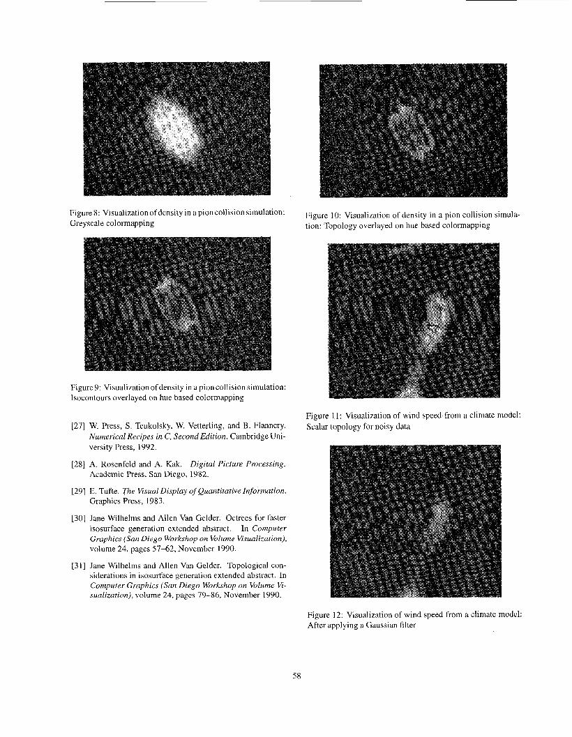
Figure 8: Visualization of density in apion collision simulation: Greyscale colormapping

Figure o: Visualization of density in a pion collision simulation: Topology overlayed on hue based colormapping

Figure9: Visualization of density in a pion collision simulatic Isocontours overlayed on hue based colormapping

3n:

Figure 11: Visualization of wind speed from a climate model: Scalar topology for noisy data W. Press, S. Teukolsky, W. Vetterling, and B. Flannery.

Numerical Recipes in C, Second Edition. Cambridge Uni- versity Press, 1992.

A. Rosenfeld and A. Kak. Digital Picture Processing. Academic Press, San Diego, 1982.

E. Tufte. The Visual Display of Quantitative Information. Graphics Press, 1983.

Jane Wilhelms and Allen Van Gelder. Octrees for faster isosurface generation extended abstract. In Computer Graphics (San Diego Workshop on Volume Visualization), volume 24, pages 57-62, November 1990.

Jane Wilhelms and Allen Van Gelder. Topological con- siderations in isosurface generation extended abstract. In Computer Graphics (San Diego Workshop on Volume Vi- sualization), volume 24, pages 79-86, November 1990.

Figure 12: Visualization of wind speed from a climate model: After applying a Gaussian filter

58

Documents

Visualization of Scalar Topology for Structural