Visual Pattern Discovery using Random Projections

Anushka Anand∗ Leland Wilkinson† Tuan Nhon Dang‡

Department of Computer Science, University of Illinois at Chicago

ABSTRACT

An essential element of exploratory data analysis is the use ofrevealing low-dimensional projections of high-dimensional data.Projection Pursuit has been an effective method for finding in-teresting low-dimensional projections of multidimensional spacesby optimizing a score function called a projection pursuit index.However, the technique is not scalable to high-dimensional spaces.Here, we introduce a novel method for discovering noteworthyviews of high-dimensional data spaces by using binning and ran-dom projections. We define score functions, akin to projection pur-suit indices, that characterize visual patterns of the low-dimensionalprojections that constitute feature subspaces. We also describe ananalytic, multivariate visualization platform based on this algorithmthat is scalable to extremely large problems.

Keywords: Random Projections, High-dimensional Data.

Index Terms: H.5.2 [User Interfaces]: Graphical user interfaces(GUI)— [H.2.8]: Database Applications—Data Mining

1 INTRODUCTION

This work is motivated by the lack of pattern detection methodsthat are efficient in high-dimensional spaces. While many of thesemethods [16, 10, 35, 28] are effective in low-dimensional spaces,their computational complexity prevents their application in veryhigh-dimensional spaces. While there are approaches to speed upthese methods [24, 49, 14], most involve parallelization schemes,computationally complex ideas or ad-hoc pre-processing methods.

By contrast, we have attempted to integrate a recent methodcalled random projections, in an iterative framework, to detect vi-sual patterns in high-dimensional spaces. The main use of the ran-dom projection theorem in data mining has been as a preprocess-ing step in order to reduce the dimensionality of a space to a man-ageable subspace before applying classification algorithms such asSupport Vector Machines or decision trees that are not readily scal-able to very high-dimensional spaces. CHIRP [46] proposed a dif-ferent approach: it is a visual-analytic classifier, based on iteratedrandom projections, that approximates the distribution-free flex-ibility of Projection Pursuit without the computational complex-ity. This motivated us to see whether guided random projectionscould be used to construct a visual analytics platform for discerningmeaningful structures in very large datasets. In this paper we inves-tigate such an approach to find dimensions that contribute stronglyto analytically meaningful features. Such features capture visualpatterns of point sets that drive substantive interpretations. Thestrength of our method is in exploiting non-axis-parallel subspaces(i.e. non-orthogonal projections).

Making this effective requires us to analyze how to visually ex-plore these random projections, as models based on subspaces, that

∗e-mail: aanand2@uic.edu†e-mail: leland.wilkinson@systat.com‡E-mail: tdang@cs.uic.edu

together characterize a score. Because we require a large num-ber of random projections to find substructures in high-dimensionalspaces, visualizing these collections of random projections to un-derstand views of the data is challenging. The Subspace Explorerwe developed incorporates multiple multivariate perspectives of thesubspace with extensive interaction and drill-down capabilities tounderstand the contribution of variables.

Our contributions in this paper are:

• An algorithmic scheme, based on random projections, to findlow-dimensional views of interesting visual substructures invery high-dimensional data.

• A methodology to compute features in high-dimensionalspace based on prior work in 2-D [47].

• An Exploratory Data Analysis (EDA) tool, the Subspace Ex-plorer, that can be used to explore multiple perspectives oflow-dimensional projections.

We describe related work in the following section. Then, we de-scribe our approach and the Subspace Explorer and finally we de-scribe our validation tests and examples of use with real data beforeending with concluding thoughts.

2 RELATED WORK

Our visual analytic application depends on several areas of prior re-search. The first concerns projections, which reduce dimensionalityin vector spaces in order to reveal structure. The second involvesmanifolds, which use graph-theoretic concepts to reveal structure inpoint distributions. The third concerns visual features, which candescribe structures in multivariate data.

2.1 Projections

To discover low-dimensional projections clearly discriminat-ing clusters, researchers have applied Multidimensional Scaling(MDS) [33] and Principle Component Analysis (PCA) [12]. Theseare computationally expensive procedures when dealing with veryhigh-dimensional data sets.

Projection pursuit has been combined with the Grand Tour [6,13], which smoothly animates a sequence of projections, resultingin a dynamic tool for EDA. Projection Pursuit has been used tofind class-separating dimensions [29] and combined with tours toinvestigate Support Vector Machines [11]. These approaches allowone to explore the data variables via projections that maximize classseparability but can only handle a small number of variables (≤ 8for clear tour displays).

Axis-parallel 2-D projections of data are ranked on a class sep-arability measure [41] for multivariate visual exploration and usedwith 1-D histograms to analyze variables and interactively constructa classifier [19]. However, using axis-parallel projections of datato find low-dimensional views with large class-separation [37] willbe ineffective when there does not exist class separability in axis-parallel views of the data.

Figure 1: Fisher’s linear discriminant separating two groups.

2.1.1 The Problem with Axis-parallel Projections

There are two serious problems with axis-parallel approaches: 1)computations on pairs of dimensions grow quadratically with thenumber of dimensions, and 2) axis-parallel projections do a poorjob of capturing high-dimensional local geometry. While the pur-suit of axis-parallel projections can be interesting and may wellwork for some smaller data sets, there is no reason to expect thatthey can reveal interesting structures in data. Moreover, the pub-lished examples of “high-dimensional” problems involve relativelyfew dimensions (in the tens or hundreds). Our Cancer dataset ex-ample has over 16,000 dimensions. Dimensions of that magnitudehave over a hundred million 2-D axis-parallel projections. Generat-ing this number of plots and visually examining them is impractical.

Regarding the second problem, consider the following worst-case lemma:

Let U be a set of p(p− 1)/2 axis-parallel unit vectorsin R

p. Let x be a p× 1 positive vector in Rp that rep-

resents a dimension of maximum interest (an interest-ing 1-D projection, a Bayes-optimal discriminating vec-tor, a first principal component, ...). Let ux be the el-ement of U that is closest in angle to x. Then for anyx, the maximum possible angle between ux and x isθmax = arccos(1/

√p).

As p increases, θmax heads toward 90 degrees rapidly (for p = 20,it’s almost 80 degrees). In short, axis-parallel projections will tendto be non-informative for high-dimensional problems. This result isa corollary of the curse of dimensionality. Thus even for algorithmsdesigned to search algorithmically through axis-parallel projectionsfor optimal views, there is no guarantee that these can be found andno way of knowing that ones discovered are anywhere near optimal.

Further, we assert that algorithms that use margins alone tofind multidimensional structure are based on mistaken assumptions.Figure 1 shows two clusters in 2-D space where neither variablealone is sufficient to determine the clusters. Fisher’s linear dis-criminant is essentially one variable that is a linear combinationof the two - the data projected onto the linear discriminant wouldclearly show two clusters. Some may argue that you get the sameresult by keeping both variables but in p-dimensional space youneed all p variables and that is impractical when dealing with large-p datasets. This point is central to every argument subsequently inthe paper. Any pattern recognition endeavor faces this problem; anexample is subspace clustering [34]. Typical papers on subspaceclustering demonstrate their value on well-separated, Gaussian orhyper-rectangle clusters in an embedding space [3, 7]. For suchdata, a directed search using greedy approaches can find these clus-ters. However, many real datasets present ill-posed problems [43].Effective modeling requires regularization techniques. Or in ourcase, random projections.

2.1.2 Random Projections

Johnson-Lindenstrauss [26] proved that if a metric on X ∈ Rp

results from an embedding of X into Euclidean space, then Xcan be embedded in R

q with distortion less than 1 + ε , where0 < ε < 1, and q = O(ε2log(|X|)). Remarkably, this embedding isachieved by projecting onto a random q-dimensional subspace suchthat, roughly speaking, the input points are projected onto spher-ically random hyperplanes through the origin. A random projec-tion matrix Tp×q ∈ R

q is generated with identical independently-distributed entries with zero mean and constant variance. This ismultiplied with the original matrix Xn×p ∈ R

p to obtain the pro-jected matrix

B =1√q

XT ∈ Rq

where q<<min(n, p). B preserves all pairwise Euclidean distancesof X in expectation. This theorem has been applied with much suc-cess to many data mining approaches from classification to cluster-ing [15, 9] primarily as a dimensionality reduction technique.

2.2 Manifolds

The manifold learning community [42, 8] has used nonlinear mapson k-Nearest Neighbor graphs to find informative low-dimensionalrepresentations of high-dimensional data. They assume that thedata of interest lie on an embedded non-linear manifold within thehigher-dimensional ambient space usually of much lower dimen-sionality. We are similarly interested in finding an embedded sub-space but instead of using geodesic distances or neighborhood func-tions to approximate high-dimensional distances, we use randomprojections.

2.3 Features

In the Rank-by-Feature framework [22], all pairwise relations areranked according to various statistical features such as correlation,uniformity, normality, etc. and users can explore 1-D or orthogo-nal 2-D views of variables using histograms, boxplots or scatter-plots. Information-bearing 2-D projections of data in scatterplotsare ranked on perceptually motivated goodness measures based onparticular tasks [5]. Albuquerque et. al [4] describe quality metricsfor multivariate visualization techniques like scatterplot matricesand parallel coordinates in relation to the related tasks of analyzingclusters and separating labeled classes. In these approaches 2-Dprojections are ranked and visually analyzed.

Turkay et al. [45] propose a model for dual analysis of itemsand dimensions through linked views of orthogonal projections ofitems and plots of summary statistics of the dimensions. The objec-tive is to understand relationships between dimensions by brush-ing items. Their work is analogous to the Scagnostics [47] idea,as they characterize and visualize individual dimensions with sum-mary statistics like the mean and skewness. In doing so, they trans-form data dimensions to feature space. By contrast, Scagnosticsis closer to the spirit of Projection Pursuit indices than restrictiveclassical statistical summaries like means and skewness. Our workextends Scagnostics as we look at characterizing visual patternswithin highly multivariate data and presenting them in an environ-ment that guides exploration.

3 THE SUBSPACE EXPLORER

In this paper we describe a computationally efficient search algo-rithm for interesting views of very high-dimensional data using anapproach based on random projections. To explore the subspacesdescribed by the discovered random projections and get insight intothe relationships between variables, we developed the Subspace Ex-plorer which leverages multiple visualizations or views of multi-variate data. To handle large datasets both in terms of n, the numberof observations, and p the number of variables, we leverage binningand random projections as described in the following sections.

3.1 Binning

To efficiently deal with large datasets in our visual analytic plat-form, we first bin datasets with more than 2000 observations. Webase the number of bins on a formula in [40]. Given n instances,we compute the marginal number of bins b using

b = c1 log2(n)

The constant c1 is a parameter the analyst can manipulate depend-ing on the level of compression required; larger values improvespeed but reduce resolution. The application defaults to c1 = 100,which is seen empirically (across a wide variety of datasets) to pro-duce a sufficiently large number of bins to capture the data dis-tribution. Multivariate data binning is usually performed by a k-Nearest Neighbor (kNN) grouping of the data or a segmentation ofthe kNN connectivity graph or a Voronoi tessellation or k-meansclustering. We adapt a single run of the k-means algorithm to findb clusters with the modification that it be sensitive to datasets withoutliers. First, we pick b data points at random as starting cen-troids, then for every data point we compute its distance to each bcentroid and store the closest centroid and distance. The goal is tohave a representative segmentation of the high-dimensional, many-points dataset, so outlier points or those far from most of the datapoints are placed into their own singleton bin. Those points whosedistance to their closest centroid is greater than a threshold t areconsidered singleton bins, where

t = µ̂ + c2σ̂

Here µ̂ is the mean of the vector of closest distances and σ̂ is thesample standard deviation of the same. The constant c2 is a tunableparameter that is set to 5 based on empirical studies that ensurethe balance between coverage and number of bins. Thus, the to-tal number of bins may increase depending on the extra singletonsdiscovered. Given the singleton bins, the other data points are as-signed to their closest bin and each bin centroid is updated. Thiscan be seen as a modified single run of the k-means algorithm withthe resulting list of bins as the segmentation of the multivariate dataspace and the bin centroids as the new data points.

3.2 Selecting Random Projections

By working with point-to-point distances in low-dimensional, non-axis-parallel subspaces, we escape the curse of dimensionality fol-lowing the successful results by researchers in the manifold learn-ing community [18]. The original Johnson-Lindenstrauss proof in-volved Gaussian weights so the input matrix X is multiplied bya dense matrix of real numbers. This is a computationally ex-pensive task for large data. Achlioptas [1] replaced those pro-jections with simpler, faster operations as he showed that usingunit-weighted projections do not jeopardize accuracy in approxi-mating distances. The projection matrix he generated consists ofidentical independently-distributed random variables with values in{1,0,−1} drawn from a probability distribution, so

ti j =√

s

1 with probability 12s

0 with probability 1− 1s

−1 with probability 12s

He recommended using s = 3 which gives a three-fold speedupas only a third of all the variables are processed to construct theembedding. The key issue for all methods producing Johnson-Lindenstauss embeddings is that it must be shown that for anyvector, the squared length of its projection is sharply concentratedaround its expected value. Achlioptas’ contribution is in determin-ing the probability distribution for the random projection matrixsuch that for all vectors the concentration is as least as good as in the

spherically symmetric case. He even shows a miniscule improve-ment while using such a spare projection matrix. The computationof the projection reduces to aggregate evaluation – summations andsubtractions of randomly selected variables but no multiplications.Furthermore, Hastie et al. [31] showed that unit random weights formost purposes can be made very sparse. For better robustness, es-pecially when dealing with heavy-tailed distributions, they recom-mend choosing s =

√p. We use this sparse formulation to produce

the projection matrix in our application.

Applying the Johnson-Lindenstrauss theorem yields a subspacewhose inter-point distances are negligibly different from the sameinter-point distances in very high-dimensional space. This enablesthe execution of relatively inefficient data mining methods withoutsignificant loss of accuracy. This also enables the fast generation oflow-dimensional projections that can be evaluated and visualized.The subspaces generated from this framework differs from the sub-spaces analyzed in traditional subspace clustering approaches [34]in that each dimension of a q-dimensional (q-D) random projection(which can individually be considered a 1-D random projection) is alinear combination of the original data dimensions. Subspace clus-tering approaches consider a subset of the original data dimensionsas the subspace to evaluate.

We generate a number, r, of random q-D projections as candidatesubspaces and score each based on the visual pattern features wedefine. Then we present the 10 top-scoring q-D random projectionsin the Subspace Explorer. For our search, we generate r = 50 q-D projections to score. We set the default q for the q-D randomprojection space to be 20. The random projection dimension q ismeant to be O(log2(n)) from the theorem, but with the binning,this is a good estimate in most cases and it can be changed by theuser of the platform easily, as needed. Generating one q-D randomprojection matrix is fast: for each 1-D random projection vector,we pick s =

√p variables and randomly assign +/− 1 weights to

them. Thus, picking redundant variables is less of a problem forrandom projections than it is for subset subspace methods. Andredundancy is less likely to occur as p increases which is the focusof this research. We then use the projection matrix to get the q-D projected data that is scored by computing features as describedbelow.

Our search strategy of generating and evaluating a random sam-ple of r subspaces has its limitations. Increasing r or the size of thesearch space, increases the likelihood of finding the desired sub-structure, but, at the cost of time. Looking at 50 high-dimensionalslices is a good compromise (which we determined empirically).Noise is another problem that plagues every data-mining algorithm.If there is a large amount of noise relative to the systematic elementsof the problem, no data mining method, including Support VectorMachines and random projection based approaches, is going to per-form well.

3.3 Computing Features

The most prevalent approaches to computing visual features inpoint sets in high-dimensional spaces have been based on 2-D axis-parallel projections [22, 5, 48]. Scagnostics [47] present a canonicalset of nine features that have proven to be effective in moderate-dimensional problems. Not all of the Scagnostics features can beextended to higher-dimensions however. Here we describe thosethat we incorporate into The Subspace Explorer. These are themeasures that are computed from the geometric Minimum Span-ning Tree (MST) of the set of points [2].

Outlying: Tukey [44] introduced a non-parametric approach tooutlier detection based on peeling the convex hull as a measure ofthe depth of a level set imposed on scattered points. We do not as-sume that the multivariate point sets are convex and want to detectoutliers that may be located in interior, relatively empty regions.So, we consider a vertex whose adjacent edges in the MST all have

a weight (length) greater than ω to be an outlier. Setting ω us-ing Tukey’s gap statistic based on conventional boxplots producesa large number of outliers for large datasets (n > 10,000). So, wdeviate from the original formula and adopt the robust methodol-ogy of Letter Value Boxplots [20] which get detailed informationin the tails through order statistics at various depths going out fromthe median. We choose the formulation of ω , the depth after whichpoints are labeled outliers, to be such that z percent of the sam-ple size are considered outliers. This z can be varied by the ana-lyst based on domain knowledge but defaults to 2%. The Outlyingmeasure is the proportion of the total edge length due to edges con-nected to detected outliers.

coutlying = length(Toutliers)/length(T )

Clumpy: This Scagnostic is based on the Hartigan and MohantyRUNT statistic [17]. The runt size of a dendrogram (the single-linkage hierarchical clustering tree) node is the smaller of the num-ber of leaves of each of the two subtrees joined at that node. Asthere is an isomorphism between a single-linkage dendrogram andthe MST, we can associate a runt size (r j) with each edge (e j) inthe MST, as described by Stuetzle [39]. The clumpy measure em-phasizes clusters with small intra-cluster distances relative to thelength of their connecting edge and ignores runt clusters with rela-tively small runt size.

cclumpy = maxj

[

1−maxk

[length(ek)]/length(e j)

]

where j indexes edges in the MST and k indexes edges in each runtset derived from an edge indexed by j.

Sparse: Sparseness measures whether points are confined to alattice or a small number of locations in the space. This can hap-pen when dealing with categorical variables or when the number ofpoints is extremely small. The 90th percentile of the distribution ofedge lengths in the MST is an indicator of inter-point closeness.

csparse = q90

Striated: Another common visual pattern is striation: parallelstrips of points produced by the product of categorical and contin-

uous variables. Let V (2) ⊆V be the set of all vertices of degree 2 inV and let I() be an indicator function. Striation counts the numberof adjacent edges whose between-angle cosine is less than -0.75.

cstriated =1

|V | ∑v∈V (2)

I(cosθe(v,a)e(v,b) <−0.75)

Stringy: With coherence in a set of points defined as the pres-ence of relatively smooth paths in the MST, a stringy shape is deter-mined by the count of degree-2 MST vertices relative to the over-all number of vertices minus the number of single-degree vertices.Smooth algebraic functions, time series, points arranged in vectorfields and curves fit this definition.

cstringy =|V (2)|

|V |− |V (1)|

3.4 Displaying Subspaces

The Subspace Explorer is an EDA dashboard that presents chartswith different views of the data and facilitates multiscale explo-ration of data subspaces through rich interactivity in a manner simi-lar to iPCA [23] which facilitates understanding the results of PCA.Others [27] have noted that connecting multiple visualizations bylinking and brushing interactions provides more information thanconsidering the component visualizations independently. We com-bine several geometric techniques - SPLOMs, parallel coordinate

plots and biplots - along with a graph-based technique and a radarplot icon to visualize collections of random projections and the sub-spaces of high-dimensional data they describe as seen in Figure 2.1.

The overall interface design of the Subspace Explorer is based onmultiple coordinated views. Each of the six data views representsa specific aspect of the input data either in dimension subspace orprojection space, and are coordinated in such a way that any inter-action with one view is immediately reflected in all the other viewsallowing the user to infer the relationships between random projec-tions and dimension subspaces. Data points are colored accordingto class labels if they exist or in a smoothly increasing gradient ofcolors from yellow to purple based on the order of the data pointsin the input file. The smooth gradient indicates the sequence of ob-servations which may be of interest when looking at Stringy shapesthat point to time series data.

Because it is designed for expert analysts, Subspace Explorertrades ease of first use for analytic sophistication. Consequentlyusers require some training to be familiarized with the definitionof random projection subspaces and to read and interact with thevarious plots. The objective of the Explorer is to aid in the interpre-tation of random projection subspaces in terms of the original datavariables. This is complicated by the fact that each dimension ofthe random projection subspace is a linear combination of a subsetof the original variables. Therefore the user can switch betweenlooking at the projected space (the q-D random projection matrixB) in the Projection Space Views and the data subspace (the subsetof dimensions used in the random projections) in the Data SpaceViews.

The Control options allow the user to select an input data file,specify whether the data file has a class label as the last column (thisinformation is used to color the data points in the visualization) anda row label as the first column, the score function to maximize, arandom number seed (for the random number generator) and thedimensionality, q, of the random projection space (the default is setto 20 as described in Section 3.2). The Update button causes thedata file to be read, the data matrix to be binned, a number of q-Drandom projections to be generated and scored, the top 10 scoringprojection scores to be shown in the Score View and the best scoringq-D projection to be shown in the Projection Space Views with thecorresponding data subspace shown in the Data Space Views.

3.4.1 Projection Space Views:

Given a selected score function, these views look at the projecteddata based on the q-D random projections that maximize the se-lected score.

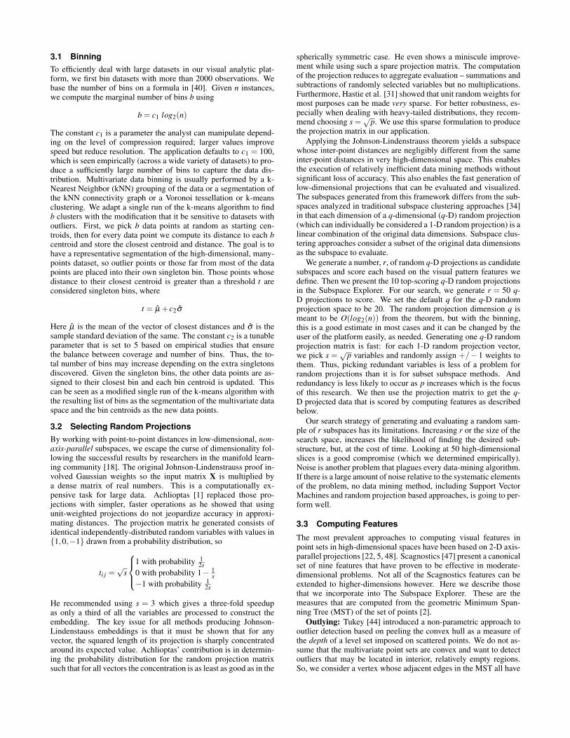
Score View:(Figure 2D) Our algorithm goes through a numberof q-D random projections and ranks them based on their scores.The default views start off with the best scoring one. It is useful totoggle through the list of a few high-scoring random projections aseach may have discovered a different view of the high-dimensionaldataset showing the interesting structure the score captured. Withvisualization tools there is not one answer or one view but rather anumber of views to look at different interesting slices or perspec-tives of the data. This barchart shows the scores of the top 10 scor-ing q-D random projections. This easily interpretable view func-tions as a controller to select a q-D random projection to investigate- selecting a bar updates all views.

Radar Plot Icon:(Figure 2E) The value of the chosen scorefunction for a selected random projection subspace is listed underthe Update button. However, the user might like to know the qualityof each subspace with respect to the other score functions. Insteadof listing the score values or providing another barchart, we use asimple visual icon to summarize the score values. The radar plot isa snapshot of the characteristics of the selected random projection

1Higher resolution images of all figures here are available at

http://www.cs.uic.edu/ aanand/subspaceExplorer.html

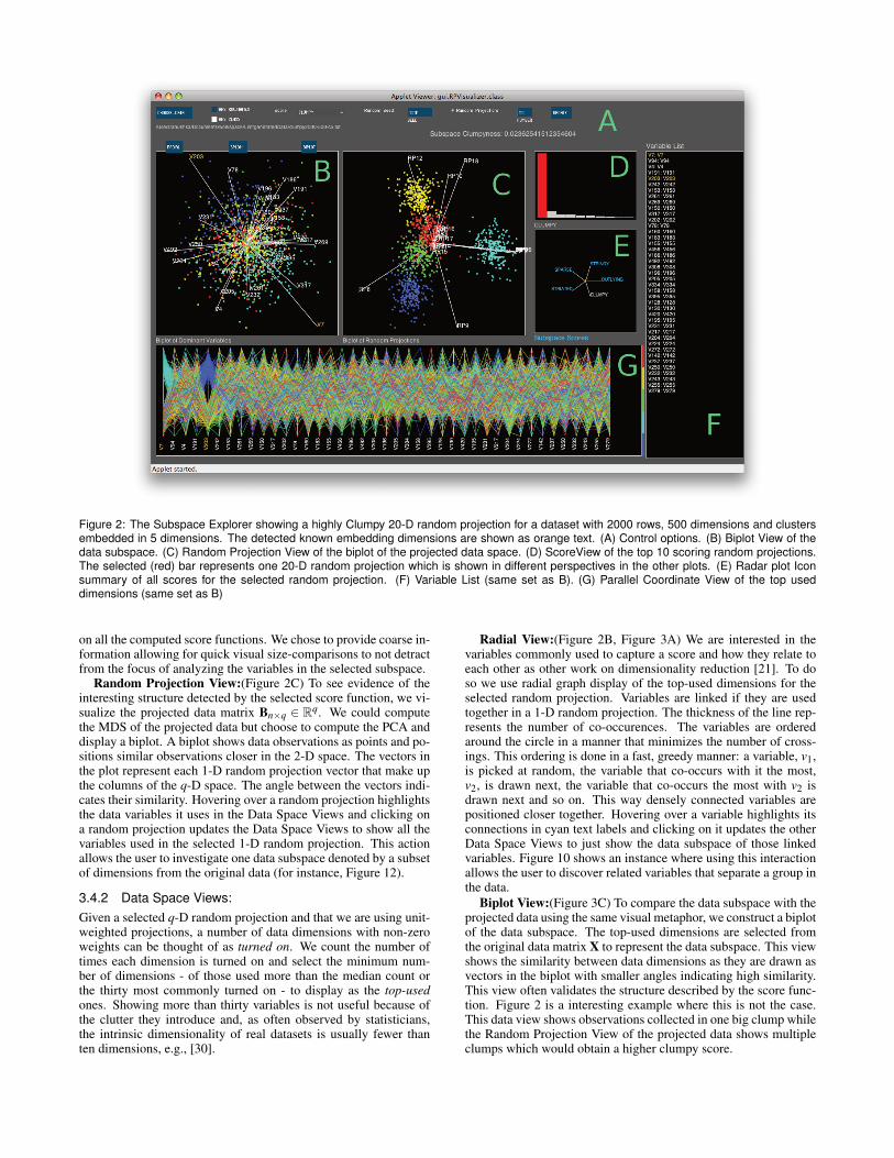
Figure 2: The Subspace Explorer showing a highly Clumpy 20-D random projection for a dataset with 2000 rows, 500 dimensions and clustersembedded in 5 dimensions. The detected known embedding dimensions are shown as orange text. (A) Control options. (B) Biplot View of thedata subspace. (C) Random Projection View of the biplot of the projected data space. (D) ScoreView of the top 10 scoring random projections.The selected (red) bar represents one 20-D random projection which is shown in different perspectives in the other plots. (E) Radar plot Iconsummary of all scores for the selected random projection. (F) Variable List (same set as B). (G) Parallel Coordinate View of the top useddimensions (same set as B)

on all the computed score functions. We chose to provide coarse in-formation allowing for quick visual size-comparisons to not detractfrom the focus of analyzing the variables in the selected subspace.

Random Projection View:(Figure 2C) To see evidence of theinteresting structure detected by the selected score function, we vi-sualize the projected data matrix Bn×q ∈ R

q. We could computethe MDS of the projected data but choose to compute the PCA anddisplay a biplot. A biplot shows data observations as points and po-sitions similar observations closer in the 2-D space. The vectors inthe plot represent each 1-D random projection vector that make upthe columns of the q-D space. The angle between the vectors indi-cates their similarity. Hovering over a random projection highlightsthe data variables it uses in the Data Space Views and clicking ona random projection updates the Data Space Views to show all thevariables used in the selected 1-D random projection. This actionallows the user to investigate one data subspace denoted by a subsetof dimensions from the original data (for instance, Figure 12).

3.4.2 Data Space Views:

Given a selected q-D random projection and that we are using unit-weighted projections, a number of data dimensions with non-zeroweights can be thought of as turned on. We count the number oftimes each dimension is turned on and select the minimum num-ber of dimensions - of those used more than the median count orthe thirty most commonly turned on - to display as the top-usedones. Showing more than thirty variables is not useful because ofthe clutter they introduce and, as often observed by statisticians,the intrinsic dimensionality of real datasets is usually fewer thanten dimensions, e.g., [30].

Radial View:(Figure 2B, Figure 3A) We are interested in thevariables commonly used to capture a score and how they relate toeach other as other work on dimensionality reduction [21]. To doso we use radial graph display of the top-used dimensions for theselected random projection. Variables are linked if they are usedtogether in a 1-D random projection. The thickness of the line rep-resents the number of co-occurences. The variables are orderedaround the circle in a manner that minimizes the number of cross-ings. This ordering is done in a fast, greedy manner: a variable, v1,is picked at random, the variable that co-occurs with it the most,v2, is drawn next, the variable that co-occurs the most with v2 isdrawn next and so on. This way densely connected variables arepositioned closer together. Hovering over a variable highlights itsconnections in cyan text labels and clicking on it updates the otherData Space Views to just show the data subspace of those linkedvariables. Figure 10 shows an instance where using this interactionallows the user to discover related variables that separate a group inthe data.

Biplot View:(Figure 3C) To compare the data subspace with theprojected data using the same visual metaphor, we construct a biplotof the data subspace. The top-used dimensions are selected fromthe original data matrix X to represent the data subspace. This viewshows the similarity between data dimensions as they are drawn asvectors in the biplot with smaller angles indicating high similarity.This view often validates the structure described by the score func-tion. Figure 2 is a interesting example where this is not the case.This data view shows observations collected in one big clump whilethe Random Projection View of the projected data shows multipleclumps which would obtain a higher clumpy score.

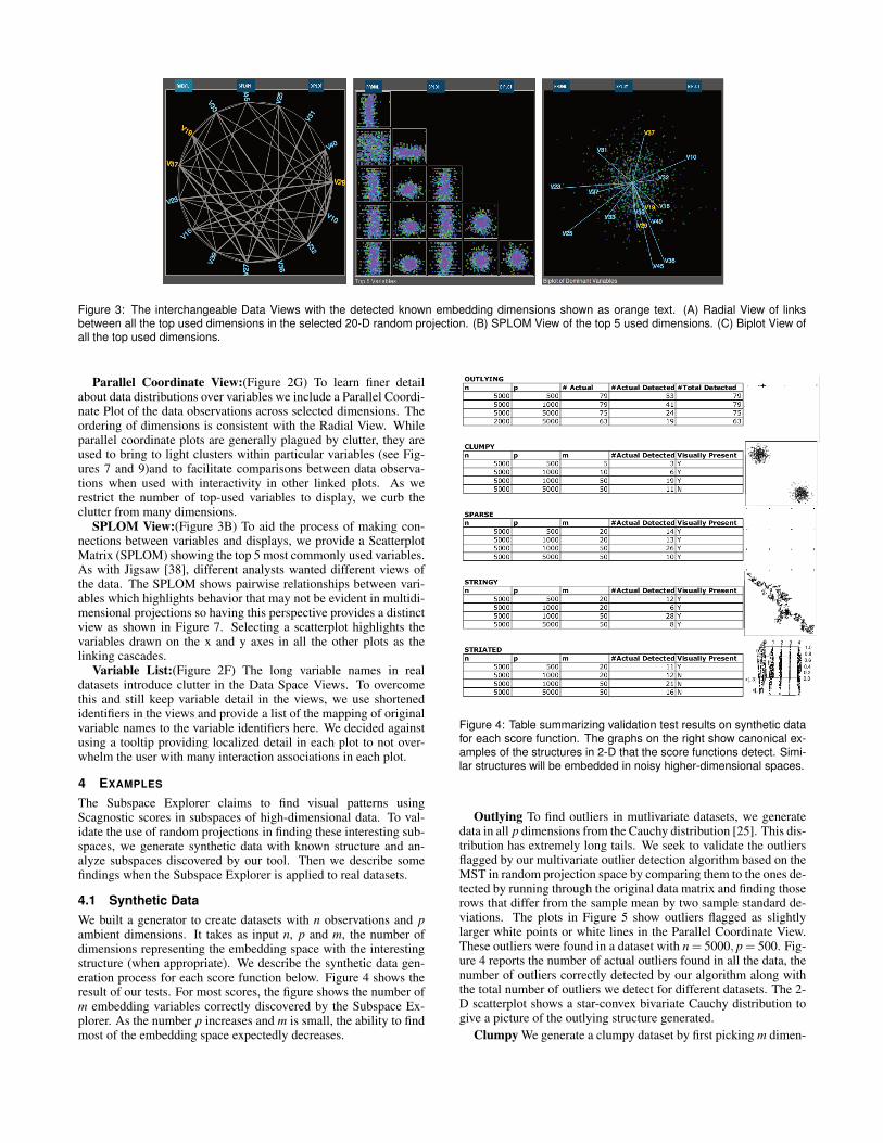
Figure 3: The interchangeable Data Views with the detected known embedding dimensions shown as orange text. (A) Radial View of linksbetween all the top used dimensions in the selected 20-D random projection. (B) SPLOM View of the top 5 used dimensions. (C) Biplot View ofall the top used dimensions.

Parallel Coordinate View:(Figure 2G) To learn finer detailabout data distributions over variables we include a Parallel Coordi-nate Plot of the data observations across selected dimensions. Theordering of dimensions is consistent with the Radial View. Whileparallel coordinate plots are generally plagued by clutter, they areused to bring to light clusters within particular variables (see Fig-ures 7 and 9)and to facilitate comparisons between data observa-tions when used with interactivity in other linked plots. As werestrict the number of top-used variables to display, we curb theclutter from many dimensions.

SPLOM View:(Figure 3B) To aid the process of making con-nections between variables and displays, we provide a ScatterplotMatrix (SPLOM) showing the top 5 most commonly used variables.As with Jigsaw [38], different analysts wanted different views ofthe data. The SPLOM shows pairwise relationships between vari-ables which highlights behavior that may not be evident in multidi-mensional projections so having this perspective provides a distinctview as shown in Figure 7. Selecting a scatterplot highlights thevariables drawn on the x and y axes in all the other plots as thelinking cascades.

Variable List:(Figure 2F) The long variable names in realdatasets introduce clutter in the Data Space Views. To overcomethis and still keep variable detail in the views, we use shortenedidentifiers in the views and provide a list of the mapping of originalvariable names to the variable identifiers here. We decided againstusing a tooltip providing localized detail in each plot to not over-whelm the user with many interaction associations in each plot.

4 EXAMPLES

The Subspace Explorer claims to find visual patterns usingScagnostic scores in subspaces of high-dimensional data. To val-idate the use of random projections in finding these interesting sub-spaces, we generate synthetic data with known structure and an-alyze subspaces discovered by our tool. Then we describe somefindings when the Subspace Explorer is applied to real datasets.

4.1 Synthetic Data

We built a generator to create datasets with n observations and pambient dimensions. It takes as input n, p and m, the number ofdimensions representing the embedding space with the interestingstructure (when appropriate). We describe the synthetic data gen-eration process for each score function below. Figure 4 shows theresult of our tests. For most scores, the figure shows the number ofm embedding variables correctly discovered by the Subspace Ex-plorer. As the number p increases and m is small, the ability to findmost of the embedding space expectedly decreases.

Figure 4: Table summarizing validation test results on synthetic datafor each score function. The graphs on the right show canonical ex-amples of the structures in 2-D that the score functions detect. Simi-lar structures will be embedded in noisy higher-dimensional spaces.

Outlying To find outliers in mutlivariate datasets, we generatedata in all p dimensions from the Cauchy distribution [25]. This dis-tribution has extremely long tails. We seek to validate the outliersflagged by our multivariate outlier detection algorithm based on theMST in random projection space by comparing them to the ones de-tected by running through the original data matrix and finding thoserows that differ from the sample mean by two sample standard de-viations. The plots in Figure 5 show outliers flagged as slightlylarger white points or white lines in the Parallel Coordinate View.These outliers were found in a dataset with n = 5000, p = 500. Fig-ure 4 reports the number of actual outliers found in all the data, thenumber of outliers correctly detected by our algorithm along withthe total number of outliers we detect for different datasets. The 2-D scatterplot shows a star-convex bivariate Cauchy distribution togive a picture of the outlying structure generated.

Clumpy We generate a clumpy dataset by first picking m dimen-

Figure 5: The Outlying score is maximized for multivariate Cauchydata and detected outliers are shown in white.

sions out of the p at random. We place cluster centroids on the mvertices of a (m− 1)-dimensional simplex. This means that a cen-troid at variable v1 for instance, would have v1 set to 1, the set of allthe other m−1 variables set to 0 and the remaining p−m variablesto be set to small Gaussian random numbers. Given the centroids,we have to generate the remaining observations. To generate a datapoint, we randomly choose a cluster this point will belong to and weadd to the centroid values small Gaussian noise. Figure 2 shows theSubspace Explorer with a dataset with n = 2000, p = 500,m = 5,so the clusters are embedded in 5 dimensions. The orange-coloredvariable names in the Data Space Views are two of the 5 variablesfrom the known embedding space. It can be seen that this viewclearly shows some clumpy sets of points which are colored by thecluster they belong to. It is important to note that simply perform-ing PCA on all the data and projecting it onto the top two principlecomponents does not reveal clusters or clumps. The 2-D scatter-plot in Figure 4 shows the clusters generated at the vertices of a1-D simplex when m = 2 and p = 2. In higher-dimensional embed-ding spaces (higher values of m), we would expect to see even moreoverlap of clusters.

Sparse To model sparseness, we first pick m dimensions outof the p at random. We set those m dimensions to have only tenunique values. The other p−m dimensions are filled with smallGaussian noise. Flipping between Projection Space views to DataSpace views can reveal subsets of the embedded space as shownin Figure 6. The Random Projection View shows some sparsitygiven the large number of noise variables in this dataset, which hasn = 5000, p = 1000,m = 50. The number of embedding space vari-ables discovered is shown in Figure 4. The scatterplot on the rightshows how points in 2-D are distributed such that each variable putspoints in four unique positions in the plane resulting in a 16-pointlattice formation.

Striated For the Striated Scagnostic we were motivated by theartifact with the RANDU pseudo-random number generator that isknown to generate points in 3-D that fall on a set of parallel 2-Dplanes [32]. For a RANDU dataset, there is a view in a narrow“squint angle” where the data are highly striated. We generatedm/2 “lattice” variables with values selected from [0.0, 0.25, 0.5,0.75, 1.0] with equal probabilities of .2. We then added m/2 “uni-form” variables sampled from a uniform distribution. Finally, weadded p−m variables sampled from the same small Gaussians weused for the other simulations. Figure 7 shows a random projec-tion with clear striation. However, as the number of Gaussian noisevariables increase, the striped structure, which is seen when a tupleof lattice and uniform variables are selected together, is not as read-

Figure 6: The Sparse score is maximized and correctly discoversthree of the variables from the embedding space, shown in orangetext.

Figure 7: The Striated score is maximized showing a clearly striatedview in this data set with n = 5000, p = 50,m = 5 where the embeddingspace is 10% of the ambient space..

ily visually discernible as noted in Figure 4. The 3-D scatterploton the right illustrates the kind of striped structure we create in theembedding space (here m = p = 4).

Stringy We generate Stringy data by constructing smooth pathsin m dimensions and embedding these in a p-dimensional space.Each observation will have a small Gaussian noise for the p−mvariables and for the m variables, we take their previous valuesand add a small amount of Gaussian noise, therefore introducinga first-order autocorrelation in the subspace. We see that the pro-jected data biplot clearly shows a stringy shape for this data set withn = 5000, p = 1000,m = 20 in Figure 8 even though the embeddingspace accounts for only 2% of the data dimensionality. Again, theprojection of all the data on the top two principle components com-pletely obscures this pattern.

4.2 Real Data

We describe two scenarios using Subspace Explorer on publicly-available, large datasets to perform EDA.

Cancer:

Figure 9 shows a high-dimensional analysis not amenable to ex-isting visual analytic platforms. There are 16,063 variables in thisdataset [36], comprising genetic markers for 14 different types of

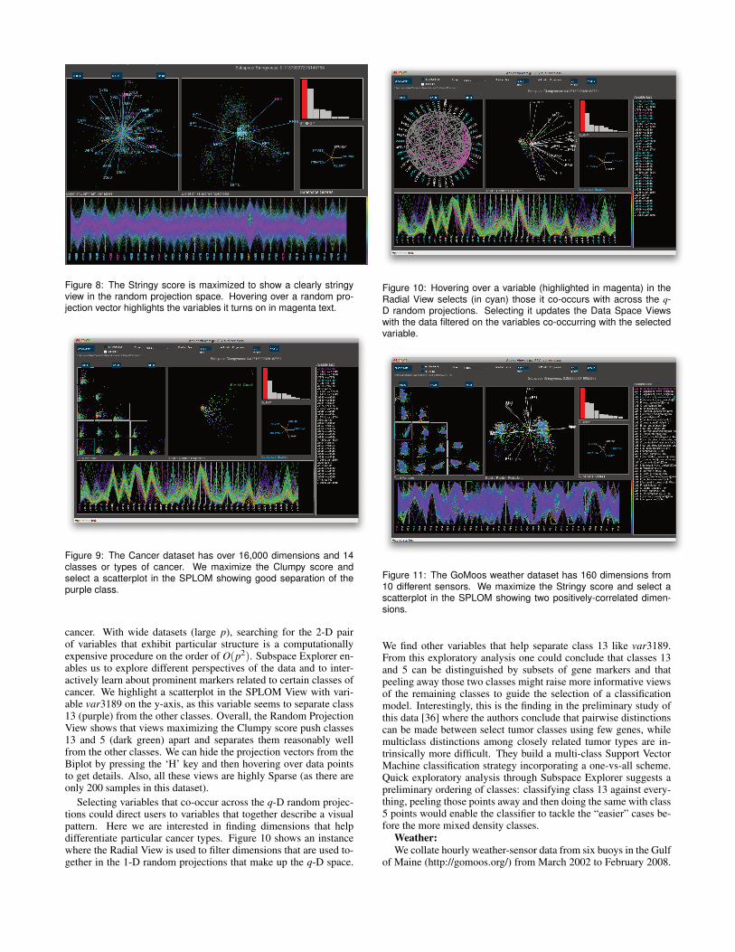
Figure 8: The Stringy score is maximized to show a clearly stringyview in the random projection space. Hovering over a random pro-jection vector highlights the variables it turns on in magenta text.

Figure 9: The Cancer dataset has over 16,000 dimensions and 14classes or types of cancer. We maximize the Clumpy score andselect a scatterplot in the SPLOM showing good separation of thepurple class.

cancer. With wide datasets (large p), searching for the 2-D pairof variables that exhibit particular structure is a computationallyexpensive procedure on the order of O(p2). Subspace Explorer en-ables us to explore different perspectives of the data and to inter-actively learn about prominent markers related to certain classes ofcancer. We highlight a scatterplot in the SPLOM View with vari-able var3189 on the y-axis, as this variable seems to separate class13 (purple) from the other classes. Overall, the Random ProjectionView shows that views maximizing the Clumpy score push classes13 and 5 (dark green) apart and separates them reasonably wellfrom the other classes. We can hide the projection vectors from theBiplot by pressing the ‘H’ key and then hovering over data pointsto get details. Also, all these views are highly Sparse (as there areonly 200 samples in this dataset).

Selecting variables that co-occur across the q-D random projec-tions could direct users to variables that together describe a visualpattern. Here we are interested in finding dimensions that helpdifferentiate particular cancer types. Figure 10 shows an instancewhere the Radial View is used to filter dimensions that are used to-gether in the 1-D random projections that make up the q-D space.

Figure 10: Hovering over a variable (highlighted in magenta) in theRadial View selects (in cyan) those it co-occurs with across the q-D random projections. Selecting it updates the Data Space Viewswith the data filtered on the variables co-occurring with the selectedvariable.

Figure 11: The GoMoos weather dataset has 160 dimensions from10 different sensors. We maximize the Stringy score and select ascatterplot in the SPLOM showing two positively-correlated dimen-sions.

We find other variables that help separate class 13 like var3189.From this exploratory analysis one could conclude that classes 13and 5 can be distinguished by subsets of gene markers and thatpeeling away those two classes might raise more informative viewsof the remaining classes to guide the selection of a classificationmodel. Interestingly, this is the finding in the preliminary study ofthis data [36] where the authors conclude that pairwise distinctionscan be made between select tumor classes using few genes, whilemulticlass distinctions among closely related tumor types are in-trinsically more difficult. They build a multi-class Support VectorMachine classification strategy incorporating a one-vs-all scheme.Quick exploratory analysis through Subspace Explorer suggests apreliminary ordering of classes: classifying class 13 against every-thing, peeling those points away and then doing the same with class5 points would enable the classifier to tackle the “easier” cases be-fore the more mixed density classes.

Weather:

We collate hourly weather-sensor data from six buoys in the Gulfof Maine (http://gomoos.org/) from March 2002 to February 2008.

Figure 12: The GoMoos weather dataset with the Data Views show-ing the subspace described by the selected 1-D random projectionRP8 (highlighted in magenta).

This results in a dataset with n = 49,000 and p = 160, as there are16 variables measured at each of the 10 buoys. We are interestedin exploring this data to discover dominant trends or relationshipsacross the spatially-distributed sensors. Figure 11 shows a highlyStringy view of a random projection of the data. Generating a listof the top 10 Stringy views of this dataset takes less than 5 seconds.This Stringy appearance is due to the presence of a subset of smoothseries within the data. The series that are relatively high-varying inthis dataset are measures related to wind-direction, wind-gust, baro-metric pressure and visibility across the multiple buoy sensors. Thebarometric pressure readings have a large number of missing valuesacross the buoys which accounts for the two clumps in the views ofthe data. The barometric pressure variables are also clearly dis-cernible in the Parallel Coordinate View as having most of the datafalling at the two extremes (for e.g. V97, V80). The SPLOM Viewallows the user to investigate correlated dimensions across buoyssuch as positively-correlated temperature readings or negatively-correlated density and temperature readings which constitute thesmooth series in the data. Figure 12 shows the Data Views updatedwith just the data subspace from the selected 1-D random projectionvector RP8. This Stringy subspace in the Biplot View is a projectionof correlated variables related to wind speed and temperature acrossmultiple buoys. The user can glean insight into natural groupings ofvariables by exploring the subspaces captured by different randomprojections and this can aid in model creation or feature selection.

4.3 Performance

Because we use efficient binning and random projections, the com-putation time for the scores based on the MST is O(log2(n)

2q)where q defaults to 20. Therefore, we can run through a largenumber of random projections quickly to find views of the high-dimensional data that maximize our score functions and show inter-esting structure. On an Intel Core 2 Duo 2.2 GHz Apple MacbookPro with 4 GB RAM running Java 1.6 and Processing 1.5.1, we runthe Subspace Explorer on different large datasets and investigate itsperformance. The graphs in Figure 13 show computation time bro-ken down into the time to read in the input data file, bin the n obser-vations, generate a list of q-dimensional random projections fromthe p dimensional data, and score the list of projections by comput-ing the MST and scores on the projected data. Empirical analysisshows that the time complexity of our approach is linear (with R2

of 0.997 for the regression fit) in n and p with the dominant timetaken to read in the data and bin it - both one pass operations. The

0 1000 2000 3000 4000 5000 6000p

0

100

200

300

Tim

e (

n=

10

00

)

SCOREGENERATEBINREAD

100

200

300

Tim

e (

n=

500

0)

100

200

300

Tim

e (

n=

100

00

)

Figure 13: Computation times (in seconds) for large datasets wheren is the number of observations and p is the number of dimensions.

largest file we read in this performance study is about 1 GB withn = 10,000, p = 5000. Thus, the Subspace Explorer is an O(np)visual analytic explorer of subspaces.

5 DISCUSSION & CONCLUSION

The Subspace Explorer was inspired by Projection Pursuit, but wemust emphasize that it does not use the Friedman-Tukey algorithm.Our approach of iteratively scoring a large list of random projec-tions to visualize high-scoring ones is efficient and ideal for vi-sually exploring very high-dimensional datasets where ProjectionPursuit or projections based on dense or sparse matrix decomposi-tions is impractical. As an alternative, many have proposed search-ing for axis-parallel projections that exhibit “interesting” structure.While these orthogonal views of variables are often found and easyto interpret, as we mentioned in Section 2.1, axis-parallel views arenot useful in finding high-dimensional structure. We look for goodnon-axis-parallel, affine, random projections that maximize a score,similar to a projection index, and visually compare the subspacesthey represent. Also, we have described scores that go beyond thecommon ones that focus on finding views showcasing clusters andoutliers. We have described a multivariate formulation of Scagnos-tic features to look for striated views where the data fall into stripes,sparse views where data fall into a few unique positions in space andstringy views where data exhibit some autocorrelation-type trend.We have identified five multivariate measures of visual structureand intend to pursue distilling additional ones. Furthermore, we areconducting user studies to investigate the intuitive use of our EDAdashboard and visual features to accomplish tasks related to featureselection.

The Subspace Explorer is a visual analytic platform facilitat-ing the exploration of collections of random projections that max-imize various score functions. The data analyst can drill-down tolook at dimensions or variables that are indicators for a score func-tion, therefore aiding in feature selection. This method of find-ing interesting views and identifying relevant dimensions in high-dimensional data is novel in that it is an implementation of iteratedrandom projections and multivariate visual pattern scores wrappedup in a visual analytic platform.

ACKNOWLEDGEMENTS

This research is supported by NSF/DHS grant DMS-FODAVA-0808860.

REFERENCES

[1] D. Achlioptas. Database-friendly random projections. In Proc. of

ACM SIGMOD, pages 274–281. ACM, 2001.

[2] P. K. Agarwal, H. Edelsbrunner, and O. Schwarzkopf. Euclidean mini-

mum spanning trees and bichromatic closest pairs. Discrete and Com-

putational Geometry, pages 407–422, 1991.

[3] R. Agrawal, J. Gehrke, D. Gunopulos, and P. Raghavan. Automatic

subspace clustering of high dimensional data for data mining applica-

tions. In Proc. of ACM SIGMOD, pages 94–105, 1998.

[4] G. Albuquerque, M. Eisemann, D. J. Lehmann, H. Theisel, and

M. Magnor. Improving the visual analysis of high-dimensional

datasets using quality measures. In Proc. IEEE VAST 2010, pages

19–26, 2010.

[5] G. Albuquerque, M. Eisemann, and M. Magnor. Perception-based

visual quality measures. In IEEE VAST, pages 13–20, 2011.

[6] D. Asimov. The grand tour: A tool for viewing multidimensional

data,. Siam Journal on Scientific and Statistical Computing, 6:128–

143, 1985.

[7] C. Baumgartner, C. Plant, K. Kailing, H.-P. Kriegel, and P. Kroger.

Subspace selection for clustering high-dimensional data. In Proc. of

the IEEE ICDM, pages 11–18, 2004.

[8] M. Belkin and P. Niyogi. Laplacian eigenmaps for dimensionality re-

duction and data representation. Neural Computation, 15:1373–1396,

2003.

[9] E. Bingham and H. Mannila. Random projection in dimensionality

reduction: applications to image and text data. In Proc. of ACM

SIGKDD, pages 245–250, 2001.

[10] B. E. Boser, I. M. Guyon, and V. N. Vapnik. A training algorithm for

optimal margin classifiers. In Proc. of COLT, pages 144–152, New

York, NY, USA, 1992. ACM.

[11] D. Caragea, D. Cook, V., and Honavar. Visual methods for examining

support vector machine results, with applications to gene expression

data analysis. Technical report, Iowa State University, 2005.

[12] J. Choo, S. Bohn, and H. Park. Two-stage framework for visualization

of clustered high dimensional data. In IEEE VAST, pages 67–74, 2009.

[13] D. Cook, A. Buja, J. Cabrera, and C. Hurley. Grand tour and projection

pursuit. Journal of Computational and Graphical Statistics, 4:155–

172, 1995.

[14] X. Z. Fern and C. E. Brodley. Random projection for high dimensional

data clustering: A cluster ensemble approach. In ICML’03, pages

186–193, 2003.

[15] D. Fradkin and D. Madigan. Experiments with random projections for

machine learning. In Proc. of ACM KDD, pages 517–522, New York,

NY, USA, 2003. ACM.

[16] J. H. Friedman and J. W. Tukey. A projection pursuit algorithm for ex-

ploratory data analysis. IEEE Transactions on Computers, C-23:881–

890, 1974.

[17] J. A. Hartigan and S. Mohanty. The runt test for multimodality. Jour-

nal of Classification, 9:63–70, 1992.

[18] C. Hegde, M. Wakin, and R. Baraniuk. Random projections for mani-

fold learning. In Neural Information Processing Systems (NIPS), Van-

couver, BC, 2007.

[19] A. Hinneburg, D. Keim, and M. Wawryniuk. Using projections to

visually cluster high-dimensional data. Computing in Science Engi-

neering, 5(2):14 – 25, 2003.

[20] H. Hofmann, K. Kafadar, and H. Wickham. Letter-value plots: Box-

plots for large data. The American Statistican, Submitted.

[21] S. Ingram, T. Munzner, V. Irvine, M. Tory, S. Bergner, and T. Mller.

Dimstiller: Workflows for dimensional analysis and reduction. In

IEEE VAST’10, pages 3–10, 2010.

[22] S. J. and B. Shneiderman. A rank-by-feature framework for interac-

tive exploration of multidimensional data. Information Visualization,

4:96–113, March 2005.

[23] D. H. Jeong, C. Ziemkiewicz, B. Fisher, W. Ribarsky, and R. Chang.

iPCA: An Interactive System for PCA-based Visual Analytics. Com-

puter Graphics Forum, 28(3):767–774, 2009.

[24] L. O. Jimenez and D. A. Landgrebe. Projection pursuit for high di-

mensional feature reduction: paralleland sequential approaches. In

Geoscience and Remote Sensing Symposium, volume 1, pages 148–

150, 1995.

[25] N. L. Johnson, S. Kotz, and N. Balakrishnan. Chapter 16. In Contin-

uous Univariate Distributions, volume 1. Wiley & Sons, 1994.

[26] W. B. Johnson and J. Lindenstrauss. Lipschitz mapping into Hilbert

space. Contemporary Mathematics, 26:189–206, 1984.

[27] D. A. Keim. Designing pixel-oriented visualization techniques: The-

ory and applications. IEEE TVCG, 6(1), 2000.

[28] J. Kruskal and R. Shepard. A nonmetric variety of linear factor anal-

ysis. Psychometrika, 39:123–157, 1974.

[29] E.-K. Lee, D. Cook, S. Klinke, and T. Lumley. Projection pursuit for

exploratory supervised classification. Journal of Computational and

Graphical Statistics, 14:831–846, 2005.

[30] E. Levina and P. J. Bickel. Maximum likelihood estimation of intrinsic

dimension. In L. K. Saul, Y. Weiss, and L. Bottou, editors, Advances

in Neural Information Processing Systems 17, pages 777–784, Cam-

bridge, MA, 2005. MIT Press.

[31] P. Li, T. J. Hastie, and K. W. Church. Very sparse random projections.

In Proc. of ACM KDD, pages 287–296, 2006.

[32] G. Marsaglia. Random numbers fall mainly in the planes. In Proc.

National Academy of Sciences, volume 61, pages 25–28, 1968.

[33] V. Osinska and P. Baia. Nonlinear approach in classification visual-

ization and evaluation. In Congress ISKO, ’09, pages 257–270, 2009.

[34] L. Parsons, E. Haque, and H. Liu. Subspace clustering for high di-

mensional data: a review. SIGKDD Explor. Newsl., 6(1):90–105, June

2004.

[35] K. Pearson. On lines and planes of closest fit to systems of points in

space. Philosophical Magazine, 2:559–572, 1901.

[36] S. Ramaswamy, P. Tamayo, R. Rifkin, S. Mukherjee, C. Yeang,

M. Angelo, C. Ladd, M. Reich, E. Latulippe, J. Mesirov, T. Poggio,

W. Gerald, M. Loda, E. Lander, and T. Golub. Multiclass cancer diag-

nosis using tumor gene expression signature. PNAS, 98:15149–15154,

2001.

[37] M. Sips, B. Neubert, J. P. Lewis, and P. Hanrahan. Selecting good

views of high-dimensional data using class consistency. Computer

Graphics Forum, 28(3):831–838, 2009.

[38] J. Stasko, C. Gorg, Z. Liu, and K. Singhal. Jigsaw: Supporting in-

vestigative analysis through interactive visualization. In Proc. of the

IEEE VAST, pages 131–138, 2007.

[39] W. Stuetzle. Estimating the cluster tree of a density by analyzing the

minimal spanning tree of a sample. Journal of Classification, 20:25–

47, 2003.

[40] H. A. Sturges. The choice of a class interval. Journal of the American

Statistical Association, 21:65–66, 1926.

[41] A. Tatu, G. Albuquerque, M. Eisemann, P. Bak, H. Theisel, M. Mag-

nor, and D. Keim. Automated analytical methods to support visual

exploration of high-dimensional data. IEEE Transactions on Visual-

ization and Computer Graphics, 17:584–597, 2011.

[42] J. B. Tenenbaum, V. de Silva, and J. C. Langford. A global geo-

metric framework for nonlinear dimensionality reduction. Science,

290(5500):2319–2323, 2000.

[43] A. N. Tikhonov and V. Y. Arsenin. Solutions of ill posed problems. V.

H. Winston and Sons, Wiley, NY, 1977.

[44] J. W. Tukey. Mathematics and the picturing of data. In Pro. of the In-

ternational Congress of Mathematicians, pages 523–531, Vancouver,

Canada, 1974. Canadian Mathematical Congress.

[45] C. Turkay, P. Filzmoser, and H. Hauser. Brushing dimensions – a

dual visual analysis model for high-dimensional data. IEEE TVCG,

17(12):2591–2599, 2011.

[46] L. Wilkinson, A. Anand, and T. Dang. Chirp: A new classifier based

on composite hypercubes on iterated random projections. In ACM

KDD, 2011.

[47] L. Wilkinson, A. Anand, and R. Grossman. Graph-theoretic scagnos-

tics. In Proc. of the IEEE Information Visualization 2005, pages 157–

164. IEEE Computer Society Press, 2005.

[48] L. Wilkinson, A. Anand, and R. Grossman. High-dimensional vi-

sual analytics: Interactive exploration guided by pairwise views of

point distributions. IEEE Transactions on Visualization and Computer

Graphics, 12(6):1363–1372, 2006.

[49] H. Zou, T. Hastie, and R. Tibshirani. Sparse principal component

analysis. Journal of Computational and Graphical Statistics, 15:2006,

2004.