Application of Random-Effects Pattern-Mixture Models for

Psychological Methods Copyright 1997 by the American Psychological Association, Inc. 1997, Vol. 2, No. 1, 64-78 1082-989X/97/$3.00

Application of Random-Effects Pattern-Mixture Models for Missing Data in Longitudinal Studies

Donald Hedeker and Robert D. Gibbons University of Illinois at Chicago

Random-effects regression models have become increasingly popular for analysis of longitudinal data. A key advantage of the random-effects approach is that it can be applied when subjects are not measured at the same number of timepoints. In this article we describe use of random-effects pattern-mixture models to further handle and describe the influence of missing data in longitudinal studies. For this approach, subjects are first divided into groups depending on their missing-data pattern and then variables based on these groups are used as model covariates. In this way, researchers are able to examine the effect of missing-data patterns on the outcome (or outcomes) of interest. Furthermore, overall estimates can be obtained by averaging over the missing-data patterns. A psychiatric clinical trials data set is used to illustrate the random-effects pattern-mixture approach to longitudinal data analysis with missing data.

Longitudinal studies occupy an important role in psychological and psychiatric research. In these studies the same individuals are repeatedly measured on a number of important variables over a series of timepoints. As an example, a longitudinal design is often used to determine whether a particular therapeutic agent can produce changes in clinical status over the course of an illness. Another application for the longitudinal study is to assess potential indicators of a change, in the subject's clinical status; for example, the assessment of whether drug plasma level measurements indicate clinical outcome.

Even in well-controlled situations, missing data in- variably occur in longitudinal studies. Subjects can be

Donald Hedeker, School of Public Health and Prevention Research Center, University of Illinois at Chicago; Robert D. Gibbons, Department of Psychiatry and School of Public Health, University of Illinois at Chicago.

We thank Nina Schooler and John Davis for use of the longitudinal data and several anonymous referees for their helpful comments. Preparation of this article was supported by National Institute of Mental Health Grant MH44826- 01A2.

Correspondence concerning this article should be ad- dressed to Donald Hedeker, Division of Epidemiology and Biostatistics (M/C 922), School of Public Health, University of Illinois at Chicago, 2121 West Taylor Street, Room 510, Chicago, Illinois 60612-7260. Electronic mail may be sent via Internet to [email protected].

missed at a particular measurement wave, with the result that these subjects provide data at some, but not all, study timepoints. Alternatively, subjects who are assessed at a given study timepoint might only provide responses to a subset of the study variables, again resulting in incomplete data. Finally, subjects might drop out of the study or be lost to follow-up, thus providing no data beyond a specific point in time.

One approach to analysis of incomplete longitudinal data is use of random-effects regression models, variants of which have been developed under a variety of names: random-effects models (Laird & Ware, 1982), variance component models (Dempster, Rubin, & Tsutakawa, 1981), hierarchical linear models (Bryk & Raudenbush, 1987), multilevel models (Goldstein, 1986), two-stage models (Bock, 1989), random coefficient models (de Leeuw & Kreft, 1986), mixed models (Longford, 1987), unbalanced repeated measures models (Jennrich & Schluchter, 1986), and random regression models (RRM; Bock, 1983a, 1983b; Gib- bons et al., 1993). Generalizations of RRM have been developed for the case of dichotomous response data (Conaway, 1989; Gibbons & Bock, 1987; Gibbons, Hedeker, Charles, & Frisch, 1994; Goldstein, 1991; Stiratelli, Laird, & Ware, 1984) and for the case of ordinal response data (Ezzet & Whitehead, 1991; Hedeker & Gibbons, 1994; Jansen, 1990). In addition to these articles, several book-length texts (Bryk & Raudenbush, 1992; Diggle, Liang, & Zeger, 1994;

64

RANDOM-EFFECTS PATtERN-MIXTURE MODELS 65

Goldstein, 1995; Longford, 1993) further describe and illustrate use of these statistical models.

An attractive and important feature of random- effects models in longitudinal data analysis is treatment of missing data. Subjects are not assumed to be measured at the same number of timepoints and, in fact, can be measured at different timepoints. Since there are no restrictions on the number of observations per individual, subjects who are missing at a given interview wave are not excluded from the analysis. The model assumes that data that are available for a given subject are representative of that subject's deviation from the average trend lines that are observed for the whole sample. The model estimates the subject's trend across time on the basis of whatever data that subject has, augmented by the time trend that is estimated for the sample as a whole and effects of all covariates in the model.

As Laird (1988) pointed out, random-effects models for longitudinal data with maximum likelihood estimation provide valid inferences in the presence of ignorable nonresponse. By ignorable nonresponse, it is meant that the probability of nonresponse is dependent on observed covariates and previous values of the dependent variable from the subjects with missing data. The notion here is that if subject attrition is related to previous performance, in addition to other observable subject characteristics, then the model provides valid statistical inferences for the model parameters. Since many instances of missing data are related to previous performance or other subject characteristics, the random-effects approach provides a powerful method for dealing with longitudinal data sets in the presence of missing data.

In longitudinal studies, ignorable nonresponse falls under Rubin's (1976) "missing at random" (MAR) assumption, in which the missingness depends only on observed data and has also been termed "random dropout" by Diggle and Kenward (1994). It is important to distinguish MAR data from what Little (1995) referred to as "covariate-dependent" dropout, in which the missing data can be explained by model covariates (the independent variables in a model) but does not depend on observed values of the dependent variable. Covariate-dependent dropout is sometimes viewed as a special case of Rubin's (1976) "missing completely at random" assumption and has also been called "completely random dropout" by Diggle and Kenward (1994). The essential distinction between MAR and covariate-dependent missing data is that in addition to allowing dependency between the missing

data and the model covariates, MAR allows the missing data to be related to observed values of the dependent variable. This distinction is important be- cause longitudinal statistical procedures like gener- alized estimating equations (GEE; Liang & Zeger, 1986) assume that the data are covariate-dependent, while full likelihood-based procedures such as the random-effects models allow for MAR data. Thus, if the missing levels of the dependent variable are thought to be related to observed previous levels of the dependent variable (e.g., subjects with very bad or very good scores drop out), then likelihood-based random-effects analysis may be valid; however, GEE analysis, in general, is not.

Recently, Little (1993, 1994, 1995) has described a general class of models dealing with missing data under the rubric of "pattern-mixture models." In particular, Little (1995) has presented a comprehensive and statistically rigorous treatment of random-effects pattern-mixture models for longitudinal data with dropouts in which the usual MAR assumption is too restrictive. In these models, subjects are divided into groups on the basis of their missing-data pattern. These groups then can be used, for example, to examine the effect of the missing-data pattern on the outcome (or outcomes) of interest. With the pattern- mixture approach, a model can be specified that does not require the missing-data mechanism to be ignorable. Also, this approach provides assessment of degree to which important model terms (i.e., Group and Group x Time interaction) depend on a subject's missing-data pattern. Overall estimates can also be obtained by averaging over the missing-data patterns.

The idea of using the missing-data pattern as a grouping variable is not new and has been proposed in many different contexts. For cross-sectional data, Co- hen and Cohen (1983, chap. 7) described this approach for missing predictor variables in multiple regression analysis. For longitudinal data, Muth6n, Kaplan, and Hollis (1987) and Allison (1987) proposed using the multiple group facilities of structural equation modeling software to estimate and contrast models for different missing-data pattern groups. Most recently, McArdle and Hamagami (1992) have demonstrated how to model latent growth structural equation models for groups on the basis of missing- data patterns. As these latter articles indicate, structural equation modeling provides a useful method for comparing and estimating longitudinal models for groups defmed by missing-data patterns.

In this article, we describe the use of random-

66 HEDEKER AND GIBBONS

effects pattern-mixture models in behavioral research and, in particular, illustrate the application and results of analysis with these techniques. In addition to illus- trating how the missing-data patterns can be used as grouping variables in the analysis, though, we also describe how overall estimates can be obtained by averaging over pattern ( "mix ing" the pattems). It should be noted that application of the pattern-mixture approach is not limited to random-effects modeling; it can also be used with other longitudinal models that allow for missing data across time (e.g., structural equation models or GEE-based models). However, we describe its use only in terms of random-effects models. Our aim is to illustrate that this combined approach provides a practical and powerful tool for analysis of longitudinal data with missing values.

A R a n d o m - E f f e c t s Regress ion Mode l for Longi tud ina l Data

Let i and k denote subjects and repeated observations, respectively. Assume that there are i = 1 . . . . . N subjects and k = 1 . . . . . ni repeated observations per subject. Let the variable tik denote the value of time (i.e., day, week, year) for the kth measurement of subject i. Further suppose that there is a between- subjects (dummy-coded) grouping factor x i that is constant across time for a given subject, for example, treatment condition with x; = 0 for the control and x i

= 1 for the experimental group. Consider the following random-effects regression model for Yik, the response of subject i at time k:

Yik = [30 + [31tik + [32xi + [33(Xi X tik )

+ Voi -t- Vl i t ik -t- Eik , (1)

where [330 is the intercept that represents in this model the value of the dependent measure at Time 0 (tik = 0) for the control group (x i = 0), [3~ is the linear effect of time for the control group, [32 is the condition difference at Time 0, and [33 is the condition difference in terms of the linear effect of time. Additionally, this model has two subject-specific effects Voi and vi i , which represent the deviation of each subject from their group intercept and linear trend, respectively. Typically, the subjects in a study and thus their cor- responding (subject specific) effects are thought to be representative of a larger population of subject effects, and so they are considered to be random, and not fixed, effects. To be treated as random effects, a form for the population distribution is specified, and

often, the normal or multivariate normal distribution is specified. In the above model, with two random effects, a bivariate normal distribution is specified for the population distribution. Finally, the model residuals ~ik are assumed to be independently distributed from a univariate normal distribution.

Some researchers have described the model given in Equation 1 in terms of a multilevel (Goldstein, 1995) or hierarchical (Bryk & Raudenbush, 1992) structure. For this, the model is partitioned into the within-subjects (or Level 1) model

Yik = boi + b l i t i k + ~ik, (2)

and between-subjects (or Level 2) model

boi = [30 + [32xi + Voi

b l i = [31 -t- [33xi -t- v i i . (3)

The between-subjects model is sometimes referred to as a s lopes as o u t c o m e s model (Burstein, Linn, & Capell, 1978). The multilevel representation shows that just as within-subjects (Level 1) covariates are included in the model to explain variation in Level 1 outcomes (Yik), between-subjects (Level 2) covariates are included to explain variation in Level 2 outcomes (the subject's intercept boi and slope bli ). Note that combining the between- and within-subjects models yields the model given in Equation 1.

More generally, the model can be written in terms of the n i × 1 vector of responses across time, Yi, of subject i:

Yi = X i ~ + Zil~i "1" Ei ( 4 )

with

Yi = the n i x 1 vector of responses for subject i, X i = a known rt i × p design matrix, I~ = a p x 1 vector of unknown population

parameters, Z; = a known r/i × r design matrix, v i = a r x 1 vector of unknown subject effects

distributed N(0, ~v), and •i = a n i × 1 vector of random residuals distributed

independently as N(0, ~Ei).

Then marginally, the Yi are distributed as independent normals with mean Xi[~ and variance--covariance matrix Z i X v Z ~ + ~ , i . With the above example, for a subject measured across four timepoints with succes- sive values of time equal to 0, 1, 2, and 3 (e.g., weeks of treatment), the matrix representation of the model is written as

RANDOM-EFFECTS PATI'ERN-MIXTURE MODELS 67

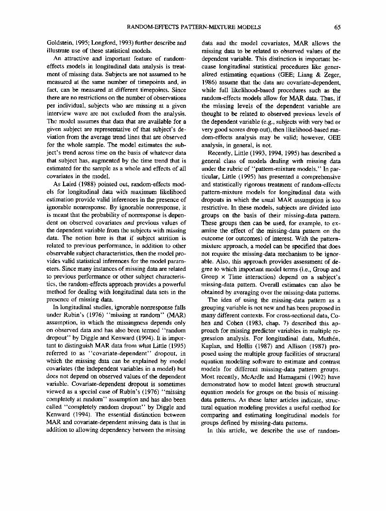
yell [moxi x/xOl[ ] [1 i] vi r ill Yi21 = 1 1 X i X i × 2 1 1 [Vli] / ~ i 2 1 Yi31 1 2 x, xi×21 + 1 + |¢ /2 l Yi4 d 1 3 X i X i X 3 d ~3 1 L ~'i4 d

Yi Xi [~i Zi vi f-i

Thus, the matrix X i contains a column of ones for the intercept, a column for the n i values of time, a column for the condition effect (which would either equal all zeros or ones since, in this example, the condition does not change over time), and a column for the product of the condition and time values. Also, as is specified in the example above, the matrix Zi would replicate the first two columns of the X i matrix, con- taining a column of ones and a column with the values of time for the subject-specific intercept and time trend deviations, respectively.

Notice that since the subject subscript i is present for the X~ and Z~ matrices, not all measurements need be made in all subjects at the same timepoints. That is, the actual values of time can vary from subject to subject (e.g., the values of the time variable for a given subject could be instead 0.5, 1.3, 1.9, and 3.1 for the four timepoints). Furthermore, since the yg vector and the X i and Z i matrices also carry the i subscript, no assumption of complete data (across timepoints) on the response or covariate measurements is being made. Thus, some subjects, for example, may have data from more or less than the four timepoints depicted in the model above. It is assumed, however, that for a given timepoint a subject has complete data on the response variable and all model covariates. Also, regarding the model residuals, it is often assumed that, conditional on the random effects, these are uncorrelated and homogeneously distributed. In that case, the simplifying assumption that ~ i =

tTEI n, × ni is made. For continuous response data, some researchers (Chi & Reinsel, 1989; Hedeker & Gibbons, 1996) have extended this model to allow for various forms of autocorrelated residuals.

With regard to parameter estimation, extensive de- tails of maximum likelihood (ML) estimation for both the continuous and dichotomous response models can be found in Longford (1993), while Hedeker and Gib- bons (1994) discussed ML estimation of the model for ordinal responses. To determine the significance of specific model parameters, one obtains large-sample

variances and covariances of the ML estimates, which can be used to construct confidence intervals and tests of hypotheses for the model parameters (Wald, 1943). Standard errors for the ML estimates are used to determine asymptotically normal test statistics (estimate divided by its standard error) for each parameter. These test statistics can then be compared with a standard normal frequency table to test the null hypothesis that a given parameter equals zero. To test for statistical difference between alternative models, one uses the likelihood-ratio X 2 test (Silvey, 1975) in certain cases. This test is appropriate when a model, Model B for example, includes all the parameters of another model, say Model A, plus some additional terms. The likelihood-ratio test compares the relative fit of the data provided by Models B and A and thus determines the significance of including these additional terms in the statistical model of the data. The significance of the additional terms in Model B is determined by comparing 2(log L n - log LA) to a table of the X 2 distribution with degrees of freedom equal to the number of additional parameters in Model B. If this likelihood ratio statistic exceeds the critical value of the ×2 distribution, the additional terms significantly improve model fit.

Pattern-Mixture Models

In a series of recent articles, Little (1993, 1994, 1995) has formulated a general class of models under the rubric "pattern-mixture models" for the analysis of missing, or incomplete, data. There have been other developments on this topic (Glynn, Laird, & Rubin, 1986; Marini, Olsen, & Rubin, 1980), as well as similar developments for specific statistical models: linear regression (Cohen & Cohen, 1983), structural equation models (Allison, 1987; McArdle & Hamagami, 1992; Muth6n et al., 1987), and random-effects models (Hogan & Laird, 1997). The recent articles by Little, however, provide a statistically rigorous and thorough treatment of these models in a general way.

The first step in applying the pattern-mixture ap-


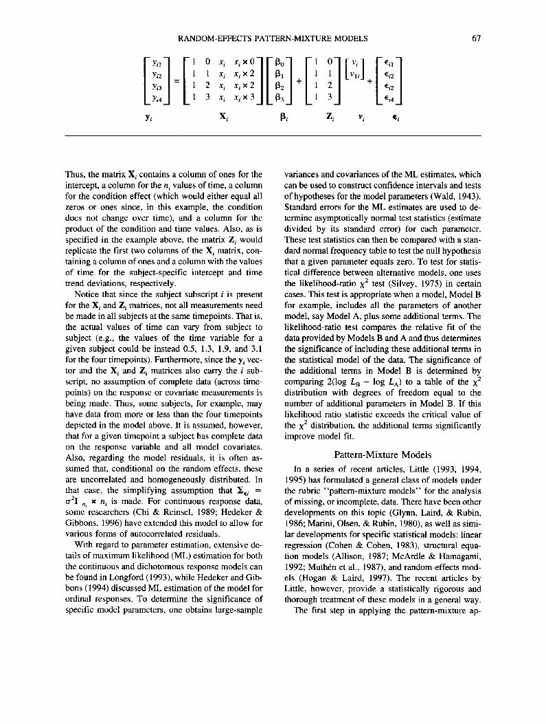
proach to handling missing data is to divide the subjects into groups on the basis of their missing-data pattern. For example, suppose that subjects are measured at three timepoints; then there are eight (23) possible missing-data patterns:

Pattern group Time 1 Time 2 Time 3 1 O O O 2 M O O 3 O M O 4 M M O 5 O O M 6 M O M 7 O M M 8 M M M

where O denotes being observed and M being missing. By grouping the subjects this way, we have cre- ated a between-subjects variable, the missing-data pattern, which can then be used in subsequent longitudinal data analysis, just as one might include a subject 's gender as a variable in the data analysis.

Next, to utilize the missing-data pattern as a grouping variable in analysis of longitudinal data, there is one important criterion: The method of analysis must allow subjects to have complete or incomplete data across time. Thus, this approach will not work with a method that requires complete data across time, since in this case, only subjects with the complete data pattern (i.e., OOO) would be included in the analysis. For example, software for a multivariate repeated measures analysis of variance usually only includes subjects with complete data across time (i.e., pattern OOO), and so using the missing-data pattern as a grouping variable is not possible. Also, since the last pattern (MMM) provides no data, for practical pur- poses, this pattern is often ignored in data analysis,

though this is not a requirement of the general pattern- mixture method (see Little, 1993). For simplicity, however, in what follows we exclude this last pattern.

In terms of including the missing-data pattern information in a statistical model, like the random- effects regression model, these seven pattems (i.e., excluding MMM from the analysis) can be repre- sented by six dummy-coded variables, for example, the (general) codings D1 to D6 given in Table 1. As given, these six dummy-coded variables represent deviations from the nonmissing pattem (OOO). Other coding schemes can be used to provide altemative comparisons among the seven pattern groups, for example, "e f fec t " or "sequential" coding (see Darling- ton, 1990, pp. 232-241, or Cohen & Cohen, 1983, chap. 5). The dummy, or effect or sequential, coded variables are then entered, for example, into a longitudinal random-effects model as a main effect and as interactions with other model variables. In this way, one can examine (a) the degree to which the groups defined by the missing-data patterns differ in terms of the outcome variable (i.e., a main effect of the missing-data pattern dummy-coded variables) and (b) the degree to which the missing-data pattern moderates the influence of other model terms (i.e., interactions with missing-data pattern). Also, from the model with the main effect and interactions of missing-data pattern, submodels can be obtained for each of the missing-dam pattern groups, and overall averaged estimates (i.e., averaging over the missing-data patterns) can be derived for the model parameters.

Modeling differences between all potential missing-data patterns may not always be possible. For example, some of the patterns, either by design or by chance, may not be realized in the sample. In some longitudinal studies, once a subject is missing at a

Table 1 Examples of Dummy-Variable Codings for Missing-Data Patterns: A Three-Timepoint Study

Dummy codes by patterns of missing data

General Monotone Last wave

Pattern D 1 D2 D3 D4 D5 D6 M 1 M2 L 1 L2 Incomplete

(Ii)

Not at final (F1)

OOO 0 0 0 0 0 0 0 0 0 0 MOO 1 0 0 0 0 0 0 0 OMO 0 1 0 0 0 0 0 0 MMO 0 0 1 0 0 0 0 0 OOM 0 0 0 1 0 0 0 1 0 1 MOM 0 0 0 0 1 0 0 1 OMM 0 0 0 0 0 1 1 0 1 0

Note. D = dummy code; O = observed; M = missing.

RANDOM-EFFECTS PATIERN-MIXTURE MODELS 69

given wave, they are missing at all later waves. In this case, the number of patterns with available data equals the number of measurement waves. For our example with three waves, the three missing-data patterns (OMM, OOM, and OOO) would then represent a monotone pattern of dropout. In this case, the two dummy-coded variables M1 and M2 given in Table 1 could be used to represent differences between each of the two dropout groups and the group of subjects observed at all t imepoints. Again, other coding schemes are possible.

Even when there are data at intermittent waves, one might want to combine some of the patterns to in- crease interpretability. For example, one might combine the patterns into groups on the basis of the last available measurement wave. For this, with three timepoints, Table 1 lists dummy codes L1 and L2 :L1 is a dummy-coded variable that contrasts those individuals who were not measured after the first timepoint with those who were measured at the last timepoint, and L2 contrasts those subjects not measured after the second timepoint with those who were measured at the last timepoint. Other recordings that may be reasonable include a simple grouping of complete data versus incomplete data, as given by contrast I1 in Table 1, or missing at the final timepoint versus available at the final timepoint, as given by contrast F1 in Table 1.

In deciding on an appropriate grouping of the missing-data patterns, a few things need to be considered. One is the sparseness of the patterns. If a pattern has very few observations, it may not make sense to treat it as a separate group in the analysis. In this case, recoding the patterns to obtain fewer groupings is reasonable. Another consideration is the potential influence of the missing-data pattern on the response variable. In longitudinal studies, it is often reasonable to assume that the intermittent missing observations are randomly missing. In this case, recoding the patterns into groups on the basis of the last available measurement wave is a sensible option. If a large percentage of subjects complete the study, it may be reasonable to simply contrast completers versus dropouts. Another consideration is whether one is interested only in estimating the main effects of the missing-data patterns or also in interactions with the missing-data patterns. For example, if one is interested in examining whether the trends across time differ by the missing-data pattern (a Missing-Data Pattern x Time interaction), it is important to realize that the patterns with only one available observation

(OMM, MOM, and MMO) provide no information for the assessment of this interaction.

Example

Psychiatric Clinical Trials

To illustrate application of the pattern-mixture approach to longitudinal data, we examined data col- lected in the National Institute of Mental Health Schizophrenia Collaborative Study on treatment- related changes in overall severity. Specifically, we examined Item 79 of the Inpatient Multidimensional Psychiatric Scale (IMPS; Lorr & Klett, 1966). Item 79, Severity of Illness, was scored as 1 = normal, not at all ill; 2 = borderline mentally ill; 3 = mildly ill; 4 = moderately ill; 5 = markedly ill; 6 = severely ill; and 7 = among the most extremely ill. Previously, we have analyzed these data (or subsets of these data) assuming a continuous scale for these 7 ordered response categories with random-effects regression (Gibbons, Hedeker, Waternaux, & Davis, 1988), di- chotomizing responses with random-effects binary probit regression (Gibbons & Hedeker, 1994), and recoding the seven ordered categories into four responses with a random-effects ordinal probit regression (Hedeker & Gibbons, 1994). In this illustration of the pattern-mixture approach, we treat this response variable as a continuous response with a random- effects regression model.

In this study, patients were randomly assigned to receive one of four medications: placebo, chlorpromazine, fluphenazine, or thioridazine. Since our previous analyses revealed similar effects for the three an- tipsychotic drug groups, they were combined in the present analysis. The experimental design and corre- sponding sample sizes are listed in Table 2.

As can be seen from Table 2, most of the measurement occurred at Weeks 0, 1, 3, and 6. However, not all subjects were observed at even these four timepoints; instead, there is evidence of appreciable dropout in this study. If we define study completion as those who were measured at Week 6, then completion

Table 2 Experimental Design and Weekly Sample Sizes

Sample size at week

Group 0 1 2 3 4 5 6

Placebo (n = 108) 107 105 5 87 2 2 70 Drug(n = 329) 327 321 9 287 9 7 265

Note. Drug = Chlorpromazine, Fluphenazine, or Thioridazine.


rates of 65% (70 of 108) and 81% (265 of 329) were observed for placebo and drug patients, respectively. This difference in study completion differs significantly between the two groups, X2(1) = 11.25, p < .001, indicating that dropout was much more pronounced for the placebo treatment group. In what follows, we are interested in examining more than just this association between dropout status and treatment group: instead, we examine the potential influence of dropout on the dependent measure, the severity of illness. In doing so, we also examine the interactive effect of dropout with time and treatment-related influences on the dependent variable.

Separate Analysis o f Completers and All Available Cases

First, let us consider a model of the changes in IMPS79 scores across time as a function of treatment group, time, and the interaction of Group x Time:

IMPS79ik = [3 o + [31(Timeik) + [32(Drug i) + [33(Drug i x Time/k) + Voi + Vli(Timeik) + ~ik. (5)

In terms of a multilevel representation, this model can be partitioned into the within-subjects model,

IMPS79ik = boi + bli(Timeik) + ~ik, (6)

and the between-subjects model,

boi = [30 + [32(Drug i) + VOi bli = [~1 + [33(Drugi) + vii. (7)

To characterize treatment group differences in this model, we use the variable Drug to represent a dummy-coded effect (placebo = 0 and drug = 1). Also, on the basis of previous analysis, to linearize the relationship of the IMPS79 scores over time, we chose a square root transformation of time; that is, the variable Time equals the square root of week (where week has values 0 thru 6). This nonlinearity of IMPS79 scores across time was characterized by a more pronounced improvement in IMPS79 scores in the initial part of the study, with a declining effect toward the end of the study. Using the square root transformation for week has the effect of assuming an equal improvement rate (i.e., an equal slope) not between weeks but, instead, between weeks 0 to 1, 1 to 4, and 4 to 9. Figure 1, which plots the observed and estimated group means (at weeks 0, 1, 3, and 6) across the square root of week, presents a reasonable linear relationship (the estimation of the group trend lines is discussed later). An alternative approach to dealing with a curvilinear trend across time would be to model IMPS79 scores in terms of both linear and quadratic time effects; however, using the square root transfor-

obs. placebo In = 107, 105, 87, 70]

obs. drug In = 327, 321, 287, 265)

- - pred. placebo

--- pred. drug

1 i i i i i i i I ~ i i i i i

-0.6 -0.2 0.2 0.6 1.0 1.4 1.8 2.2 2.6

Week [in square r o o t unite)

Figure 1. Mean Inpatient Multidimensional Psychiatric Scale, Item 79 (IMPS79), across time and treatment group; obs. = observed; pred. = predicted.


mation has the advantage of using only one parameter for the effect of time and one for the Group x Time interaction.

With this characterization of the drug and time effects, one can interpret the regression parameters as follows: [30 represents the average IMPS79 score at Week 0 for the placebo (Drug = 0) group; [31 represents the average trend across time (sq rt week) for the placebo group; [32 represents the average difference in IMPS79 scores at Week 0 between the drug and pla-

cebo groups; and [33 represents the average difference in trend lines between the drug and placebo groups. Furthermore, this model allows for each person to deviate from the group trend line in terms of the in-

tercept (Voi) and trend across time (vii). This random-effects regression model was first fit

including only completers (i.e., only the 335 subjects who were measured at Week 6) and then re-estimated with all 437 subjects. Estimates from the latter analysis were used to construct the predicted regression lines in Figure 1, and as can be seen, the model fits the observed means well. Parameter estimates are presented in the first two sets of columns in Table 3. Conclusions based on these two analyses agree in terms of indicating that the treatment groups do not significantly differ at baseline, that the placebo group does improve over time, and that the drug group has greater improvement over time in relation to the placebo group. However, the estimates of the regression parameters, though similar, do suggest some differ-

ences. A more thorough examination is now under- taken to characterize and assess the significance of these differences.

A Comparison o f Completers Versus Dropouts

For this, let us define a variable Dropout with two values: 0 if the person was measured at Week 6 (completers) and 1 if the person was not measured at Week 6 (dropouts). Dividing subjects into these two groups is a simple characterization of the missing-data patterns; however, it provides a direct way of assessing whether subjects who completed the study were similar to those who did not. Figures 2a and 2b, respectively, plot the observed and estimated group means at Weeks 0, 1, 3, and 6 (in sqrt week units) for the completers and the dropouts (the est imated group trend lines are discussed below). The plots suggest that the improvement rate of drug as compared with placebo is more pronounced among those subjects who dropped out then among the completers. A possible interpretation of this is that dropout occurred for different reasons for the two groups: For the placebo subjects, dropouts were those exhibiting the least response to treatment, while for the drug group the dropouts had the quickest and most pronounced response to treatment.

To examine this possibil i ty in a more formal man- ner, let us augment the model given by Equation 5 in the following way:

Table 3 NIMH Schizophrenia Collaborative Study: Severity of lllness (IMPS79) Across Time (N = 437), RRM Parameter Estimates (Est.), Standard Error (SE), and p Values

Completers (N = 335) All subjects (N = 437) Pattern mixture (N = 437)

Parameter Est. SE p< Est. SE p< Est. SE p<

Intercept 5.221 .109 .001 5.348 .088 .001 5.221 .108 .001 Time (sqrt week) -.393 .073 .001 -.336 .068 .001 -.393 .076 .001 Drug (0 = placebo; 1 = drug) .202 .123 .10 .046 .101 .65 .202 .121 .10 Drug x Time -.539 .083 .001 -.641 .078 .001 -.539 .086 .001 Dropout (0 = no; 1 = yes) .320 .186 .09 Dropout x Time .252 .159 .12 Dropout x Drug -.399 .227 .08 Dropout x Drug x Time -.635 .196 .002 Intercept variance .398 .068 .369 .060 .361 .060 Intercept-Time covariance -.011 .035 .021 .034 .012 .033 Time variance .205 .031 .242 .032 .230 .032 - 2 log L 3782.1 4649.0 4623.3

Note. p values are not given for variance and covariance estimates (see Bryk & Raudenbush, 1992 p. 55). NIMH = National Institute of Mental Health; RRM = random regression models; IMPS79 = Inpatient Multidimensional Psychiatric Scale, Item 79.


A

b ~

B

obs. placebo (n = 69, 68, 67, 70]

obs. drug (n = 263, 260, 253, 265)

- - pred. placebo

- - - pred. d rug

1 i i i i I i I i i I i I -0 .6 -0 .2 0.2 0.6 1.0 1.4 1.8 2.2 2.6

Week [in square r o o t unite)

A

I D obs. placebo (n = 64, 61, 34)

obs. drug (n = 38, 37, 20]

- - pred. placebo

i - - - pred. drug

1 i i i I i i i L I i I i i

-0.6 -0.2 0.2 0.6 1.0 1.4 1.6 2.2 2.6

Week [in square r o o t uni ts ]

Figure 2. completers and (b) time and treatment group for dropouts; obs. = observed; pred. = predicted.

Mean Inpatient Multidimensional Psychiatric Scale, Item 79 (IMPS79), across (a) time and treatment group for

IMPS79ik = 130 + 131(Timeik) + 132(Drugi) + 133(Drugi X Time/k) + 84(Dropouti) + 135(Dropouti x Time/k ) + 136(Dropouti X Drug/) + 137(Dropouti × Drug i × Tim%) -}- 1)Oi "~- Vli(Timeik) + ~'ik ( 8 )

Note that for a multilevel representation, the within- subjects model is the same as that in equation 6; however, the between-subjects model is now given as

boi = 8o + 132(Drugi) + 134(Dropouti) + 136(Dropouti x Drug/) + Voi

bli = 81 -I" 83(Drugi) + 135(Dropouti) + 137(Dropouti × Drug/) + vii. (9)

Here, with the coding of the variables, Drug, Dropout, and Time as described, the regression coefficients 130 and 131 represent the intercept and trend for the placebo completers (both Drug and Dropout equal zero),

RANDOM-EFFECTS PATTERN-MIXTURE MODELS 73

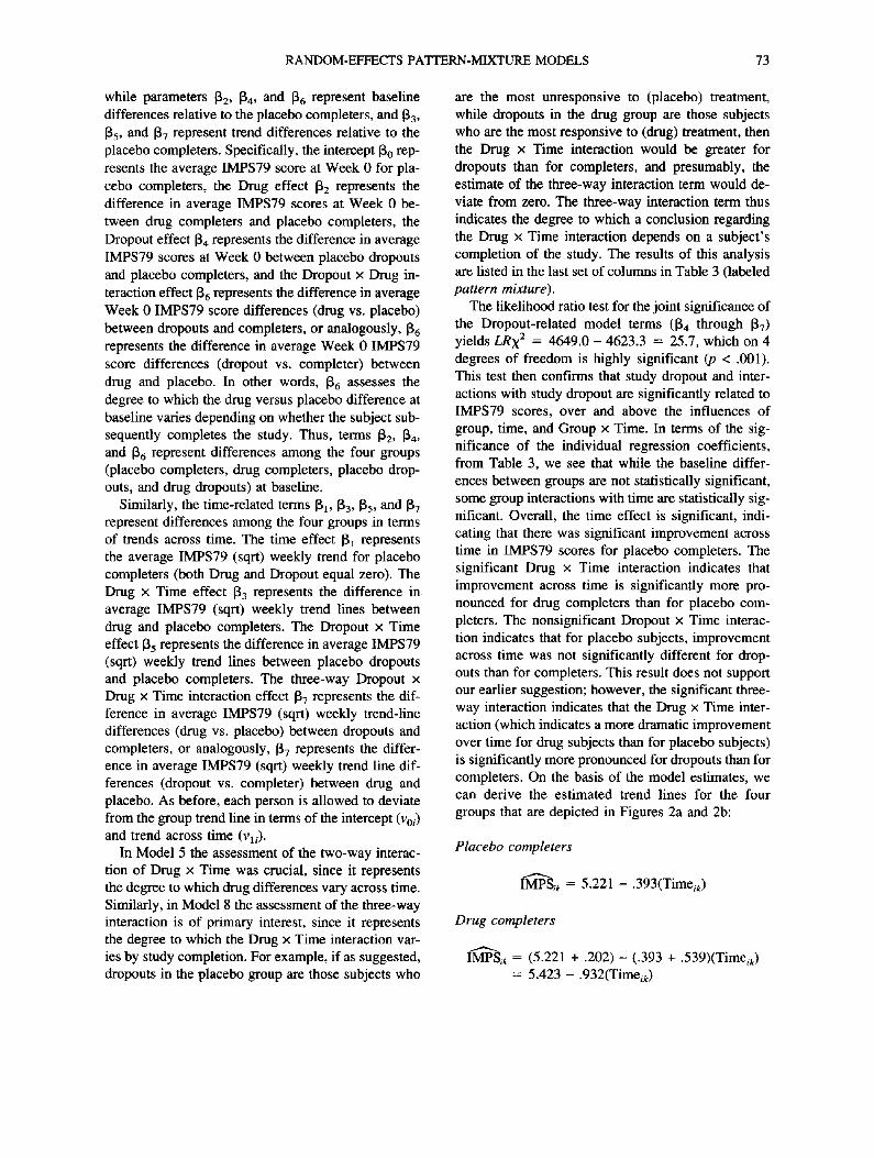
while parameters [32, [34, and [36 represent baseline differences relative to the placebo completers, and [33, [35, and [37 represent trend differences relative to the placebo completers. Specifically, the intercept [30 represents the average IMPS79 score at Week 0 for placebo completers, the Drug effect [32 represents the difference in average IMPS79 scores at Week 0 between drug completers and placebo completers, the Dropout effect [34 represents the difference in average IMPS79 scores at Week 0 between placebo dropouts and placebo completers, and the Dropout × Drug interaction effect [36 represents the difference in average Week 0 IMPS79 score differences (drug vs. placebo) between dropouts and completers, or analogously, [36 represents the difference in average Week 0 IMPS79 score differences (dropout vs. completer) between drug and placebo. In other words, [36 assesses the degree to which the drug versus placebo difference at baseline varies depending on whether the subject sub- sequently completes the study. Thus, terms [32, [34, and [36 represent differences among the four groups (placebo completers, drug completers, placebo dropouts, and drug dropouts) at baseline.

Similarly, the time-related terms [31, [33, [35, and [37 represent differences among the four groups in terms of trends across time. The time effect [31 represents the average IMPS79 (sqrt) weekly trend for placebo completers (both Drug and Dropout equal zero). The Drug × Time effect [33 represents the difference in average IMPS79 (sqrt) weekly trend lines between drug and placebo completers. The Dropout × Time effect [35 represents the difference in average IMPS79 (sqrt) weekly trend lines between placebo dropouts and placebo completers. The three-way Dropout × Drug × Time interaction effect [37 represents the difference in average IMPS79 (sqrt) weekly trend-line differences (drug vs. placebo) between dropouts and completers, or analogously, [37 represents the difference in average IMPS79 (sqrt) weekly trend line differences (dropout vs. completer) between drug and placebo. As before, each person is allowed to deviate from the group trend line in terms of the intercept (Vo/) and trend across time (vii).

In Model 5 the assessment of the two-way interaction of Drug × Time was crucial, since it represents the degree to which drug differences vary across time. Similarly, in Model 8 the assessment of the three-way interaction is of primary interest, since it represents the degree to which the Drug x Time interaction varies by study completion. For example, if as suggested, dropouts in the placebo group are those subjects who

are the most unresponsive to (placebo) treatment, while dropouts in the drug group are those subjects who are the most responsive to (drug) treatment, then the Drug × Time interaction would be greater for dropouts than for completers, and presumably, the estimate of the three-way interaction term would deviate from zero. The three-way interaction term thus indicates the degree to which a conclusion regarding the Drug × Time interaction depends on a subject's completion of the study. The results of this analysis are listed in the last set of columns in Table 3 (labeled pattern mixture).

The likelihood ratio test for the joint significance of the Dropout-related model terms ([34 through [37) yields LRx 2 = 4649.0 - 4623.3 = 25.7, which on 4 degrees of freedom is highly significant (p < .001). This test then confirms that study dropout and interactions with study dropout are significantly related to IMPS79 scores, over and above the influences of group, time, and Group × Time. In terms of the significance of the individual regression coefficients, from Table 3, we see that while the baseline differences between groups are not statistically significant, some group interactions with time are statistically significant. Overall, the time effect is significant, indicating that there was significant improvement across time in IMPS79 scores for placebo completers. The significant Drug × Time interaction indicates that improvement across time is significantly more pronounced for drug completers than for placebo completers. The nonsignificant Dropout × Time interaction indicates that for placebo subjects, improvement across time was not significantly different for dropouts than for completers. This result does not support our earlier suggestion; however, the significant three- way interaction indicates that the Drug × Time interaction (which indicates a more dramatic improvement over time for drug subjects than for placebo subjects) is significantly more pronounced for dropouts than for completers. On the basis of the model estimates, we can derive the estimated trend lines for the four groups that are depicted in Figures 2a and 2b:

Placebo completers

IMPSik = 5.221 -.393(Timeik)

Drug completers

I~"Sik = (5.221 + .202) - (.393 + .539)(Timeik ) = 5 . 4 2 3 - .932(Timeik )


Placebo dropouts

IMPS,., = (5.221 + .320) - (.393 - .252)(Timeik) = 5.541 - .141(Timeik)

Drug dropouts

IMPSa = (5.221 + .202 + .320 - .399) - (.393 + .539 - .252 + .635)(Timeik)

= 5 . 3 4 4 - 1.315(Timeik )

These estimated trend lines fit the observed means very well and illustrate that although all groups start the study, on average, between markedly and severely ill (i.e., between IMPS79 values of 5 and 6), the estimated improvement rate over time depends on both the treatment and completion status. In particular, the estimated improvement rate is most pronounced for dropouts in the drug treatment and least pronounced for dropouts in the placebo treatment.

Thus far, the analysis has indicated that the treatment effect across time varies by completion status. An additional step in the pattern-mixture approach is necessary to yield overall population estimates averaging over the missing-data patterns. Little (1993, and 1995) and Hogan and Laird (1997) discussed this step of averaging over pattern to yield estimates for the whole population, and Dawson and Lagakos (1993) and Dawson (1994) described an approach for obtaining an overall statistical test comparing treatment groups that are stratified on missing-data pattern. In the present case, on the basis of the final model, we can obtain estimates for the four fixed effects (Inter- cept, Time, Drug, and Drug x Time) separately for completers,

[~c) = [5 .221- .393 .202- .539] ' , (10)

and for dropouts,

~(a~ = 13(c) + [.320.252 -.399 -.635]' = [5 .541- .141- .197-1 .174] ' . (11)

Averaged estimates for these four parameters (de- noted ~g) are then equal to

= "rr~)~¢c) + "rr(a)[3 (a), (12)

where ~(¢) and ~r (d) represent the population weights for completers and dropouts, respectively. Although these weights are not usually known, they can be estimated by the sample proportions (335/437 and 102/ 437 for completers and dropouts, respectively). This yields

= [5 .296- .335 .109- .687] ' (13)

as the averaged overall estimates. To obtain corre- sponding estimates of the standard errors for these overall estimates, the delta method as described in Hogan and Laird (1997) can be used:

,fr(C),fr (d) ^ + N ([3(hc) - ~(ff))2' (14)

where h = 1,2,3,4 denotes the four fixed effects, N = 437 is the total number of subjects, and V(l~h) denotes the estimate of the variance of [3 h (i.e., the square of its estimated standard error). The last term in the sum is the contribution to the variance that is added be- cause the proportion of completers (and dropouts) is estimated in the sample. The estimated standard errors for these four overall terms are then .090, .067, .103, and .079.

As a slightly more sophisticated approach, the estimated proportions of completers and dropouts can be obtained when stratified by treatment group, yielding estimated proportions of, respectively, (70/108) and (30/108) for placebo and (265/329) and (64/329) for drug. Using these estimated proportions is akin to stating that study completion varies by, or depends on, treatment group. As it was shown earlier that completion did vary by treatment group for this study, these stratified estimates for the missing-data pattern groups are probably more reasonable than are the overall marginal proportions. Using these as estimates yields overall estimates:

= [5.334-.305 .124- .662] ' , (15)

with estimated standard errors as .089, .071,. 105, and .078.

Either of these sets of overall estimates and accom- panying standard errors, which are obtained by averaging over the missing-data patterns, is very similar to those obtained from the RRM analysis that ignores the missing-data patterns (i.e., from the RRM analysis of all 437 subjects presented in the second set of columns in Table 3). In particular, using any of these sets of estimates and standard errors yields nearly identical z statistics (i.e., estimate divided by its standard error) for these four model parameters and the same conclusions: significant differences from zero for all parameters except the drug effect (i.e., the drug difference at baseline). Thus, for this example, the pattern-mixture model provides the same general conclusion in terms of the overall treatment group trends across time. However, it also reveals the mixture of trends that

RANDOM-EFFECTS PATYERN-MIXTURE MODELS 75

exist on the basis of the missing-data patterns (i.e., dropouts and completers) within each treatment group.

Discussion

Since missing values in longitudinal studies are more often the norm than the exception, it is important for the data analyst to consider various alterna- tives for longitudinal data analysis with missing values. A naive approach might be to ignore subjects with incomplete data and model only those subjects measured at all timepoints. Clearly, this approach can only be reasonable to the extent that these two groups of subjects (those with and without missing values) do not systematically differ. However, subjects with missing values are often quite different from those subjects with complete data, and so an analysis that focuses exclusively on the latter group suffers from a selection problem: The population that is being gen- eralized to is not the full population but rather the subpopulation with characteristics only of the complete-data subjects. Furthermore, even in the unlikely case that the two groups are not different, an analysis that ignores some of the available data is not an effi- cient analysis, yielding underpowered statistical tests.

Analysis using random-effects models goes further in providing a realistic model for both subjects with complete and incomplete data. The assumption of ignorable nonresponse (Laird, 1988)--that the missing data are missing at random, conditional on both model covariates and observed values of the dependent vari- a b l e - i s often reasonable, and so the statistical tests provided by these models remain valid. In this article, we have illustrated how to augment these random- effects models by including variables defined by a subject's pattern of missing data. In so doing, a model can be specified that does not require the missing-data mechanism to be ignorable. Also, the pattern-mixture approach provides assessment of degree to which (the influence of) model terms vary by the missing-data patterns and provides a way of obtaining estimates, averaging over the missing-data patterns. In our example, we considered a very simple characterization of the pattern-mixture approach, focusing on only one aspect of the missing-data patterns: Was the subject measured at the last study timepoint or not? Though simple, it was clearly able to account for the differ- ential association between study dropout and symp- tom severity for the two condition groups (drug and placebo). By using a simple example of the pattern-

mixture approach, we highlighted the accessibility of this approach. Clearly, a simple, yet sensible, approach to handling the missing data is better than simply ignoring them and hoping for the best.

The complexity of the approach taken may depend on the amount of missing data. For example, if a study has only a handful of subjects with missing data across time, it may not matter, in practical terms, whether the subjects with missing data are ignored or included as a group in the analysis. Clearly, the statistical power for detecting effects (i.e., main effects and interactions) due to missing-data patterns are lower, all other things being equal, as the numbers of subjects in those patterns are reduced. In other words, an effect or interaction due to missing-data pattern group is more likely to be detected, all other things being equal, the more missing data there are. While it is difficult to give general guidelines for the treatment of missing-data patterns in a given analysis (i.e., number of missing-data patterns or grouping together of missing-data patterns), the considerations are similar to those encountered when dealing with other between-subjects grouping variables.

Besides the pattern-mixture approach, other methods have been proposed to handle missing data in longitudinal studies (Diggle & Kenward, 1994; Heck- man, 1976; Heyting, Tolboom, & Essers, 1992; Leigh, Ward, & Fries, 1993). Many of these alternative approaches are termed selection models and in- volve two stages that are performed either separately or iteratively. The first stage is to develop a predictive model for whether or not a subject drops out with variables obtained prior to the dropout, often the variables measured at baseline. This model of dropout provides a predicted dropout probability or propensity for each subject; these dropout propensity scores are then used in the (second stage) longitudinal data model as a covariate to adjust for the potential influence of dropout. By modeling dropout, selection models provide valuable information regarding the predictors of study dropout; however, an advantage of pattern-mixture models is that they can be used even when no such predictors are available. Further discussion on some of the differences between pattern- mixture and selection models can be found in Glynn et al. (1986), Little (1993, 1994, 1995), and the discussion section of the Diggle and Kenward (1994) article.

In this article, we have focused on the situation in which the dependent variable is missing across time. Alternatively, in some studies, some of the explana-


tory variables may be missing either at baseline or across time. The use of dummy variables has also been proposed for situations involving missing explanatory variables (Cohen & Cohen, 1983); however a recent article (Jones, 1996) has called this approach into question. Little (1992) describes more general methods for dealing with missing explanatory variables.

Methods for appropriately handling missing data are increasingly being developed, allowing researchers the ability to more effectively deal with this potential threat to validity. With this in mind, it is important that researchers consider the reasons for missing data in their own data sets and to choose among statistical methods with these reasons in mind. In doing so, researchers can address the issue of how well the statistical model they are using represents both the observed and the unobserved data.

R e f e r e n c e s

Allison, P. D. (1987). Estimation of linear models with incomplete data. Sociology Methodology, 1987, 71-103.

Bock, R. D. (1983a). The discrete Bayesian. In H. Wainer & S. Messick (Eds.), Modern advances in psychometric research (pp. 103-115). Hillsdale, NJ: Erlbaum.

Bock, R.D. (1983b). Within-subject experimentation in psychiatric research. In R. D. Gibbons & M. W. Dysken (Eds.), Statistical and methodological advances in psychiatric research (pp. 59-90). New York: Spectrum.

Bock, R. D. (1989). Measurement of human variation: A two stage model. In R. D. Bock (Ed.), Multilevel analysis of educational data (pp. 319-342). New York: Academic Press.

Bryk, A. S., & Raudenbush, S.W. (1987). Application of hierarchical linear models to assessing change. Psycho- logical Bulletin, 101, 147-158.

Bryk, A. S., & Raudenbush, S. W. (1992). Hierarchical linear models: Applications and data analysis methods. Newbury Park, CA: Sage.

Bryk, A. S., Raudenbush, S. W., & Congdon, R. T. (1994). Hierarchical linear modeling with the HLM/2L and HLM/3L programs. Chicago: Scientific Software, Inc.

Burstein, L., Linn, R. L., & Capell, I. (1978). Analyzing multi-level data in the presence of heterogeneous within- class regressions. Journal of Educational Statistics, 4, 347-389.

Chi, E. M., & Reinsel, G. C. (1989). Models for longitudinal data with random effects and AR(1) errors. Journal of the American Statistical Association, 84, 452-459.

Cohen, J., & Cohen, P. (1983). Applied multiple regression/

correlation analysis of the behavioral sciences (2nd ed.). Hillsdale, NJ: Erlbaum.

Conaway, M.R. (1989). Analysis of repeated categorical measurements with conditional likelihood methods. Jour- nal of the American Statistical Association, 84, 53~51.

Darlington, R.B. (1990). Regression and linear models. New York: McGraw-Hill.

Dawson, J. D. (1994). Stratification of summary statistics tests according to missing data patterns. Statistics in Medicine, 13, 1853-1863.

Dawson, J. D., & Lagakos, S. W. (1993). Size and power of two-sample tests of repeated measures data. Biometrics, 49, 1022-1032.

de Leeuw, J., & Kreft, I. (1986). Random coefficient models for multilevel analysis. Journal of Educational Statistics, 11, 57-85.

Dempster, A. P., Rubin, D. B., & Tsutakawa, R. K. (1981). Estimation in covariance component models. Journal of the American Statistical Society, 76, 341-353.

Diggle, P., & Kenward, M. G. (1994). Informative dropout in longitudinal data analysis (with discussion). Applied Statistics, 43, 49-94.

Diggle, P., Liang, K.-Y., & Zeger, S. L. (1994). Analysis of longitudinal data. New York: Oxford University Press.

Ezzet, F., & Whitehead, J. (1991). A random effects model for ordinal responses from a crossover trial. Statistics in Medicine, 10, 901-907.

Gibbons, R. D., & Bock, R. D. (1987). Trend in correlated proportions. Psychometrika, 52, 113-124.

Gibbons, R. D., & Hedeker, D. (1994). Application of random-effects probit regression models. Journal of Con- sulting and Clinical Psychology, 62, 285-296.

Gibbons, R. D., Hedeker, D., Charles, S. C., & Frisch, P. (1994). A random-effects probit model for predicting medical malpractice claims. Journal of the American Sta- tistical Association, 89, 760-767.

Gibbons, R. D., Hedeker, D., Elkin, I., Watemaux, C., Krae- mer, H. C., Greenhouse, J. B., Shea, M. T., Imber, S. D., Sotsky, S. M., & Watkins, J. T. (1993). Some conceptual and statistical issues in analysis of longitudinal psychiatric data. Archives of General Psychiatry, 50, 739-750.

Gibbons, R. D., Hedeker, D., Watemaux, C., & Davis, J. M. (1988). Random regression models: A comprehensive approach to the analysis of longitudinal psychiatric data. Psychopharmacology Bulletin, 24,438--443.

Glynn, R. J., Laird, N. M., & Rubin, D. B. (1986). Selection modeling versus mixture modeling with nonignorable nonresponse. In H. Wainer (Ed.), Drawing inferences from self-selected samples (pp. 115-142). New York: Springer-Verlag.

Goldstein, H. (1986). Multilevel mixed linear model analy-


sis using iterative generalised least squares. Biometrika, 73, 43-56.

Goldstein, H. (1991). Nonlinear multilevel models, with an application to discrete response data. Biometrika, 78, 45-51.

Goldstein, H. (1995). Multilevel statistical models (2nd ed.). New York: Halstead Press.

Heckman, J. (1976). The common structure of statistical models of truncation, sample selection, and limited dependent variables and a simple estimator for such models. Annals of Economic and Social Measurement, 5, 475- 492.

Hedeker, D., & Gibbons, R. D. (1994). A random-effects ordinal regression model for multilevel data. Biometrics, 50, 933-944.

Hedeker, D., & Gibbons, R. D. (1996). MIXREG: A computer program for mixed-effects regression analysis with autocorrelated errors. Computer Methods and Programs in Biomedicine, 49, 229-252.

Heyting, A., Tolboom, J. T. B. M., & Essers, J. G. A. (1992). Statistical handling of drop-outs in longitudinal clinical trials. Statistics in Medicine, 11, 2043-2061.

Hogan, J. W., & Laird, N. M. (1997). Mixture models for the joint distribution of repeated measures and event times. Statistics in Medicine 16, 239-258.

Jansen, J. (1990). On the statistical analysis of ordinal data when extravariation is present. Applied Statistics, 39, 75-84.

Jennrich, R. I., & Schluchter, M. D. (1986). Unbalanced repeated-measures models with structured covariance matrices. Biometrics, 42, 805-820.

Jones, M. P. (1996). Indicator and stratification methods for missing explanatory variables in multiple linear regression. Journal of the American Statistical Association, 91, 222-230.

Laird, N. M. (1988). Missing data in longitudinal studies. Statistics in Medicine, 7, 305-315.

Laird, N. M., & Ware, J. H. (1982). Random-effects models for longitudinal data. Biometrics, 38, 963-974.

Leigh, J. P., Ward, M. M., & Fries, J. F. (1993). Reducing attention bias with an instrumental variable in a regression model: Results from a panel of rheumatoid arthritis patients. Statistics in Medicine, 12, 1005-1018.

Liang, K.-Y., & Zeger, S.L. (1986). Longitudinal data analysis using general ized est imating equations. Biometrika, 73, 13-22.

Little, R. J. A. (1992). Regression with missing X's: A re-

view. Journal of the American Statistical Association, 87, 1227-1237.

Little, R. J. A. (1993). Pattern-mixture models for multivariate incomplete data. Journal of the American Statis- tical Association, 88, 125-133.

Little, R. J. A. (1994). A class of pattern-mixture models for normal incomplete data. Biometrika, 81,471-483.

Little, R. J. A. (1995). Modeling the drop-out mechanism in repeated-measures studies. Journal of the American Sta- tistical Association, 90, I 112-1121.

Longford, N. T. (1986). VARCL---Interactive software for variance component analysis: Applications for survey data. Professional Statistician, 5, 28-32.

Longford, N. T. (1987). A fast scoring algorithm for maximum likelihood estimation in unbalanced mixed models with nested random effects. Biometrika, 74, 817- 827.

Longford, N.T. (1993). Random coefficient models. New York: Oxford University Press.

Lorr, M., & Klett, C. J. (1966). Inpatient Multidimensional Psychiatric Scale: Manual. Palo Alto, CA: Consulting Psychologists Press.

Marini, M. M., Olsen, A. R., & Rubin, D. B. (1980). Maxi- mum-likelihood estimation in panel studies with attrition. Sociology Methodology, 1980, 314-357.

McArdle, J. J., & Hamagami, F. (1992). Modeling incomplete longitudinal and cross-sectional data using latent growth structural models. Experimental Aging Research, 18, 145-166.

Muth6n, B., Kaplan, D., & Hollis, M. (1987). On structural equation modeling with data that are not missing completely at random. Psychometrika, 52, 431-462.

Rasbash, J., Wang, M., Woodhouse, G., & Goldstein, H. (1995). MLn: Command reference guide. London: Insti- tute of Education, University of London.

Rubin, D. B, (1976). Inference and missing data. Biomet- rika, 63, 581-592.

Silvey, S. D. (1975). Statistical inference. New York: Chap- man and Hall.

Stiratelli, R., Laird, N. M., & Ware, J. H. (1984). Random effects models for serial observations with binary response. Biometrics, 40, 961-971.

Wald, A. (1943). Tests of statistical hypotheses concerning several parameters when the number of observations is large. Transactions of the American Mathematical Soci- ety, 54, 426--482.

(Appendix follows on next page)


A p p e n d i x

C o m p u t e r I m p l e m e n t a t i o n W i t h S A S P R O C M I X E D

A listing of the SAS PROC MIXED program that was used to obtain the random-effects regression estimates presented in this article is included. Prior to the PROC MIXED analyses, subjects are classified as either completers or dropouts. For this, the maximum value of the WEEK variable for each subject is obtained using PROC MEANS. Then a subject is classified as a completer if their maximum WEEK value is equal to 6 (DROPOUT = 0) or as a dropout if it is less than 6 (DROPOUT = 1). Data sets are then merged to combine the DROPOUT subject-level variable with the other variables and also to create a data set for completers only. Three PROC MIXED analyses are run: (a) for all subjects ignoring the DROPOUT status, (b) for subjects who completed the study only, and (c) the pattern- mixture model including DROPOUT as a covariate, including interactions. In all three analyses, the intercepts and slopes due to time are treated as random (i.e., subject- varying) terms. This same analysis can also be performed with other software that performs random-effects analysis, for example, the BMDP 5V procedure, HLM (Bryk, Raudenbush, & Congdon, 1994), MIXREG (Hedeker & Gibbons, 1996), MLn (Rasbash, Wang, Woodhouse, & Goldstein, 1995) and VARCL (Longford, 1986). Additional work is necessary to obtain the pattern-mixture averaged results: the SAS IML program used to obtain the pattern- mixture averaged results and the data for this example can be obtained from World Wide Web site http://www.uic.edu/ -hedeker/mix.html.

TITLE1 'Random-effects analysis of NIMH Schizophrenia longitudinal data'; DATA ONE; INFILE 'C:kDATAX,schizrep.dat'; INPUT ID IMPS79 WEEK DRUG SEX;

/* The coding for the variables is as follows: ID = subject ID number IMPS79 = overall severity (1 = normal, 2 = borderline mentally ill, 3 = mildly ill, 4 = moderately ill, 5 = markedly ill, 6 = severely ill, 7 = among the most extremely ill) WEEK = 0, I, 2, 3, 4, 5, 6 (most of the obs. are at weeks 0,1,3, and 6) DRUG 0 = placebo 1 = drug (chlorpromazine, fluphenazine, or thioridazine) S E X 0 = female 1 = ma le* /

/* compute square root of WEEK to linearize relationship */ SWEEK = SQRT(WEEK);

/* calculate the maximum value of WEEK for each subject (suppress the printing of the output for this procedure)*/

PROC MEANS NOPRINT; CLASS ID; VAR WEEK; OUTPUT OUT = TWO MAX = MAXWEEK; RUN;

/* determine if a subject has data at WEEK 6 DROPOUT = 0 (for completers) or = 1 (for dropouts) */ DATA THREE; SET TWO; DROPOUT = 0; IF MAXWEEK LT 6 THEN DROPOUT = 1;

/* data set with all subjects (adding the DROPOUT variable) */ DATA FOUR; MERGE ONE THREE; BY ID; /*data set with completers only (present at WEEK 6) */ DATA FIVE; MERGE ONE THREE; BY ID; IF DROPOUT EQ 0;

TITLE2 'Analysis on All Subjects'; PROC MIXED DATA = FOUR METHOD = ML; CLASS ID; MODEL IMPS79 = SWEEK DRUG DRUG*SWEEK / SOLUTION; RANDOM INTERCEPT SWEEK / SUB = ID TYPE = UN G; RUN;

TITLE2 'Analysis on Completers Only'; PROC MIXED DATA = FIVE METHOD = ML; CLASS ID; MODEL IMPS79 = SWEEK DRUG DRUG*SWEEK / SOLUTION; RANDOM INTERCEPT SWEEK / SUB = ID TYPE = UN G; RUN;

TITLE2 'Analysis on All Subjects - Pattern-Mixture Model'; PROC MIXED DATA = FOUR METHOD = ML; CLASS ID; MODEL IMPS79 = SWEEK DRUG DRUG*SWEEK

D R O P O U T D R O P O U T * S W E E K DROPOUT*DRUG DROPOUT*DRUG*SWEEK / SOLUTION;

RANDOM INTERCEPT SWEEK / SUB = ID TYPE = UN G; RUN;

Rece ived July 10, 1995

Revis ion rece ived Sep tember 20, 1996

Accep ted Sep tember 25, 1996 •

Documents

Application of Random-Effects Pattern-Mixture Models for