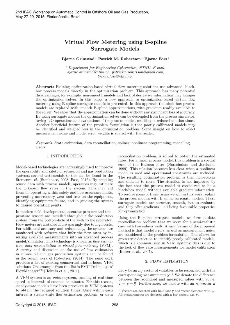
Virtual Flow Metering using B-splineSurrogate Models

Bjarne Grimstad ∗ Patrick M. Robertson ∗ Bjarne Foss ∗

∗Department for Engineering Cybernetics, NTNU. E-mail:bjarne.grimstad@ntnu.no, patrickm.robertson@gmail.com,

bjarne.foss@ntnu.no.

Abstract: Existing optimization-based virtual flow metering solutions use advanced, black-box process models directly in the optimization problem. This approach has many potentialdisadvantages, for example: non-smooth models and lack of derivative information may hamperthe optimization solver. In this paper a new approach to optimization-based virtual flowmetering using B-spline surrogate models is presented. In this approach the black-box processmodels are replaced with smooth B-spline approximations, with gradients readily available tothe solver. We show that the approximation can be done without any significant loss of accuracy.By using surrogate models the optimization solver can be decoupled from the process simulator,saving I/O-operations and evaluations of the process model, resulting in reduced solution times.Another beneficial feature of the problem formulation is that poorly calibrated models maybe identified and weighed less in the optimization problem. Some insight on how to selectmeasurement noise and model error weights is shared with the reader.

Keywords: State estimation, data reconciliation, splines, nonlinear programming, modellingerrors.

1. INTRODUCTION

Model-based technologies are increasingly used to improvethe operability and safety of subsea oil and gas productionsystems; several testimonials to this can be found in theliterature, cf. (Stenhouse, 2008; Foss, 2012). By couplingsensor data with process models, operators may estimatethe unknown flow rates in the system. This may aidthem in: operating within safety and flow assurance limits,preventing unnecessary wear and tear on the equipment,identifying equipment failure, and in guiding the systemto desired operating points.

In modern field developments, accurate pressure and tem-perature sensors are installed throughout the productionsystem, from the bottom-hole of the wells to the separator.Flow meters are installed more sparingly due to high costs.For additional accuracy and redundancy, the systems aremonitored with software that infer the flow rates by in-serting available measurements into an advanced processmodel/simulator. This technology is known as flow estima-tion, data reconciliation or virtual flow metering (VFM).A survey and discussion on the use of flow estimationin subsea oil and gas production systems can be foundin the recent work of Robertson (2014). The same workprovides a list of existing commercial and in-house VFMsolutions. One example from this list is FMC Technologies’FlowManagerTM(Holmas et al., 2011).

A VFM system is an online system, running at real-timespeed in intervals of seconds or minutes. For this reason,steady-state models have been prevalent in VFM systemsto obtain the required solution times. Once within eachinterval a steady-state flow estimation problem, or data

reconciliation problem, is solved to obtain the estimatedrates. For a linear process model, this problem is a specialcase of the Kalman filter (Narasimhan and Jordache,1999). This relation becomes less clear when a nonlinearmodel is used and operational constraints are included.The resulting optimization problem is then non-convexand difficult to solve. The situation is not improved bythe fact that the process model is considered to be ablack-box model without available gradient information.To resolve some of these issues we will in this work replacethe process models with B-spline surrogate models. Thesesurrogate models are accurate, smooth, fast to evaluate,and they offer gradients – all being favourable propertiesfor optimization.

Using the B-spline surrogate models, we form a datareconciliation problem that we solve for a semi-realisticcase with two subsea wells. A nice feature of the proposedmethod is that model errors, as well as measurement noise,are considered in the problem formulation. This allows forgross error detection to identify poorly calibrated models,which is a common issue in VFM systems; this is due tothe lack of flow rate measurements for model calibration(Bieker et al., 2007).

2. FLOW ESTIMATION

Let y be an ny-vector of variables to be reconciled with thecorresponding measurements y. 1 We denote the differencebetween the reconciled and measured values with v, i.e.v = y − y. Furthermore, we denote with an nx-vector x

1 Vectors are denoted with bold face y and vector elements with yi.All measurements are denoted with a bar accent, e.g. y.

2nd IFAC Workshop on Automatic Control in Offshore Oil and Gas Production,May 27-29, 2015, Florianópolis, Brazil

Copyright © 2015, IFAC 298

the unmeasured variables that we want to estimate. Toestimate x we solve the following nonlinear programmingproblem

minimizex,y,v,w

||v||2M + ||w||2Nsubject to g(x,y) = w

y − y = v

x ∈ X

(P)

where g : Rnx × Rny → Rm are m maps between thereconciled (measured) variables y and the unmeasuredvariables x. In general, g is a vector of nonlinear functionsand, hence, g(·) = w describes a nonconvex constraintset. The variables w ∈ Rm represent model errors; inthe case of a perfect model w = 0. The set X is aconvex polytope which may include linear constraints onthe estimated variables x. Note that the measurements yare not considered variables in P.

The objective of P is a weighted least-squares quadraticfunction defined by the norms ||v||2M = vTMv and||w||2N = wTNw, representing penalties on measurementand modelling errors, respectively. The matrices M andN can be thought of as the inverse covariance matrices forthe measurement noise and model errors. In this work weset M = diag(µ) and N = diag(ν), where µ and ν aretwo vectors of non-negative weights, to obtain diagonal,positive definite matrices and a convex objective function.

Problem P is a steady-state data reconciliation problem.Next we describe how P may be configured to estimatethe flow rates in a simple subsea production system withtwo wells. The sequential solution of this problem, incor-porating new measurements as they become available, isoften termed virtual flow metering.

2.1 Formulating a simple flow estimation problem

Here we present a configuration of P which can be appliedto any two-well subsea template tied back through a singlepipeline (see Fig. 1). Extensions to include more wellsand/or more complex topologies are straightforward.

For a subsea production system the vector of measuredvariables is typically y = [pT, tT,uT]T, with measurementsy = [pT, tT, uT]T, where p denotes pressures, t denotestemperatures, and u denotes choke openings. The unmea-sured variables to be estimated are typically the flow rates,i.e. x = q, where q denotes the flow rates. The vectorg may include pressure and temperature drop functions,as well as other relations between the variables. Below,we consider some commonly used pressure drop functions.For simplicity we assume perfect temperature and chokeopening measurements and fix t = t and u = u in theformulation.

The well performance is usually described by the inflowperformance relationship (IPR) which describes the inflowfrom the reservoir to the wellbore. The IPR depends onfactors such as rock properties (e.g. permeability), fluidproperties, the well completion, et cetera, and relates the

liquid rate qliqi to the flowing bottom hole pressure pbh

i :

wipri = gipr

i (pbhi , q

liqi ) = pbh

i − f ipri (qliq

i ), ∀ i ∈ {A,B}. (1)

The vertical lift performance (VLP) curve describes therelationship between the well flow and the pressure loss

Fig. 1. Topology of production system.

from the bottom hole to the wellhead, and depends on e.g.the well geometry and fluid properties. While a well canbe modelled from the reservoir to the wellhead using theIPR and VLP curve, the two models can be combined tocreate a single well performance curve (WPC)

wwpci = pwh

i − fwpci (qliq

i ), ∀ i ∈ {A,B}. (2)

The VLP curve may be ambiguous with respect to flowrate due to gas lifting at low flow rates, therefore we preferto use the WPC, which is usually more well-behaved.

Wellhead choke valves control the flow rates from eachwell. The flow rates through the choke valves depend one.g. choke geometry and the upstream flow regime.

wchki = pman − f chk

i (qliqi , p

whi ; twh

i , ui), ∀ i ∈ {A,B}. (3)

The wellhead choke model used in this paper is a multipliermodel, which is based on the simple valve equation to-gether with a Morris multiphase multiplier and Chisholmslip correlation (see e.g. Schuller et al. (2003)).

The flowline is modelled using the OLGAS 3P multiphaseflow correlation. The input variables to the correlation areupstream (manifold) pressure, liquid flow rate, gas-oil ratio(GOR) and water cut (WCT). The measured upstreamtemperature is considered a fixed parameter. The outputis the downstream (separator) pressure:

wfl = psep − ffl(pman, qliqC , r

gorC , rwct

C ; tman). (4)

For convenience, we collect all the model errors in a vector

w =[wipr

A , wiprB , w

wpcA , wwpc

B , wchkA , wchk

B , wfl]>

,

with corresponding weights ν. Similarly, we collect themeasurement/reconciliation errors in a vector

v =[vbhA , v

bhB , v

whA , vwh

B , vman, vsep]>,

with corresponding weights µ.

In addition to the pressure drop constraint functions in g,we model interrelations between the unmeasured variablesx with the constraint set X. For example, we include massbalance constraints on the rate variables q in X, e.g.

qpC = qpA + qpB , for p ∈ {oil, gas,wat}.Other linear relations that we include in X are:

qliqi = qoil

i + qwati , qgas

i = rgori qoil

i , qwati = rwct

i qliqi ,

for i = {A,B}, where rgori and rwct

i are a constant GORand WCT, respectively.

IFAC Oilfield 2015May 27-29, 2015

Copyright © 2015, IFAC 299

3. B-SPLINE SURROGATE MODELS

In practice, the nonlinear maps in g, such as the pressureloss functions in the previous section, are given by someprocess simulator. Most commercially available processsimulators are proprietary code and may be consideredas “black-box calculators”. A process simulator modelsthe production network with complex, nonlinear functionsthat may be non-smooth in certain regions. Generally,no derivative information is made available and finitedifference methods must be used when optimizing withgradient-based solvers, often resulting in a large number ofevaluations. Furthermore, when coupling an optimizationsolver to a (black-box) process simulator, evaluation maybe time consuming for several reasons: 1. the simulatormay require convergence of the whole network model ateach evaluation (even when perturbing a single componentof the network), and 2. the IO-operations to transfer databetween the solver and simulator may be time consuming.To solve the above problems we will replace the nonlinearmaps g with B-spline approximations φ. The B-splines inφ are referred to as B-spline surrogate models.

Note that the pressure drop functions in the previoussection are on the form gi(·) = yi − fi(·) = wi. Thus,in the following we will approximate fi (instead of gi) byφi, i.e. φi ≈ fi, and gi ≈ yi − φi.

3.1 B-splines

A B-spline is a piecewise polynomial function in thevariable x, defined by a degree p, a vector of knots t ∈Rn+p+1, and a vector of n coefficients c ∈ Rn as follows:

φ(x; p, t) = cTb(x; p, t). (5)

b(x; p, t) ∈ Rn is a vector of n B-spline basis functions.The basis functions are overlapping, degree p, polynomialfunctions, as depicted in Fig. 2 for n = 8 and p = 3. Thebasis functions and their derivatives may be evaluated bythe numerically stable and fast, recursive algorithms ofDe Boor (1972) and Cox (1972).

0 1 2 3 4 50

0.2

0.4

0.6

0.8

1

x

b i(x)

Fig. 2. B-spline basis functions for p = 3 and n = 8.

The B-spline in (5) generalizes to the multivariate case,where it is called the tensor product B-spline. Most prop-erties of the univariate B-spline, such as a high degree ofsmoothness and local support, carry over to the multivari-ate case without any complications. For brevity we willdiscuss only univariate B-splines in the rest of this section.We note however that the discussion is valid also for tensorproduct B-splines. The interested reader is referred to thetextbooks of Schumaker (1981) and Piegl and Tiller (1997)for an introduction to multivariate splines.

3.2 Cubic spline interpolation

Let any function f : R → R, for example fwpcA in

(2), be sampled on a regular (rectangular) grid to yieldN data points {xi, f(xi)}Ni=1. Several methods exist forconstructing a B-spline that interpolates these N points.These methods vary in how the B-spline degree p andknots t are selected. The commonly preferred cubic spline(p = 3) can be obtain by using a free end conditions knotvector

tF = { x1, . . . , x1︸ ︷︷ ︸p+1 repetitions

, x3, . . . , xm−2, xm, . . . , xm︸ ︷︷ ︸p+1 repetitions

}.

To obtain the spline the following linear system is solvedfor the coefficients c:

[b(x1) b(x2) . . . b(xN )]T︸ ︷︷ ︸

B

c = f , (6)

where f = [f(xi)]Ni=1 and B ∈ RN×n is called the B-spline

collocation matrix. Note that b(x) = b(x; 3, tF ) in (6).

One advantage with (cubic) spline interpolation is that itavoids the problem of Runge’s phenomenon, in which os-cillation occurs between the interpolation points (as is ev-ident in interpolation with high degree polynomials). Thefunctions in g are often polynomial or near-polynomial andapproximated by B-splines with little error. The authors’experience with approximating various pressure loss func-tions suggests that the approximation error typically lies inthe order of 0.1 − 0.001% (in fact, the error can be madearbitrarily small by increasing the sampling resolution).Arguably, the error between g and reality is orders ofmagnitude larger than this. To illustrate this with anexample, let φwpc

N (qliq) be the B-spline approximation ofthe WPC fwpc(qliq) sampled in N points. Further, leteN (qliq) = 1−φwpc

N (qliq)/fwpc(qliq) be the resulting relativeapproximation error. Approximation errors for N = 50,N = 10 and N = 5 are shown in Figure 3, while errormeasures are summarized in Table 1.

0 100 200 300 400

0

0.5

1

Liquid rate [Sm3/h]

Relativeerror[%

] e50 (50 samples)

e10 (10 samples)

e5 (5 samples)

Fig. 3. B-spline approximation errors for a WPC.

Table 1. Maximum errors and 2-norms.

N ‖eN‖∞ ‖eN‖25 1.1 · 10−2 7.8 · 10−2

10 6.1 · 10−4 5.7 · 10−3

50 6.5 · 10−5 2.4 · 10−4

The construction of a B-spline surrogate model is a two-step procedure: 1. sampling the simulator and 2. solvingthe linear system in (6) for the B-spline coefficients. Thisprocedure can be run offline and the resulting B-splinesstored in advance of optimizing P.

IFAC Oilfield 2015May 27-29, 2015

Copyright © 2015, IFAC 300

4. RESULTS AND DISCUSSION

4.1 Reference OLGA simulation

To test the performance of the estimator, a production net-work model representative to Figure 1 was implemented inOLGA, which is considered the de facto industry standardfor dynamic simulation of multiphase petroleum produc-tion systems (Bendiksen et al., 1991; Schlumberger, 2014).A benchmarking simulation was run to obtain a set ofnoise-free measurements {yk}Tk=0 (pressures, temperaturesand choke positions) and flow rates {qk}Tk=0, which wereassumed to be unknown. Here, k are time indices (thesimulation was run for 26 hours with a 10 second samplinginterval). In the simulation, the choke valves were sequen-tially stepped up from 5 % to 60 % opening, as depictedin Figure 4. Default OLGA settings were used.

0 5 10 15 20 25

20

40

60

Time [h]

Chokeposition[%

]

Well A

Well B

Fig. 4. Choke positions.

4.2 Obtaining the pressure drop models

To equip the estimator with the necessary pressure dropmodels, a model of the production network was im-plemented in Petroleum Experts’ IPM software package(Petroleum Experts Ltd, 2014). IPRs, WPCs and theflowline model were sampled from the IPM module GAP,and approximated with cubic B-splines. For the chokes, weused a multiplier model based on the valve equation, whichwas also sampled and approximated with B-splines. Priorto sampling, the models were matched against multi-rateflow tests run in OLGA. The IPRs, WPCs and flowlinemodel were matched using available tools in GAP, whilethe choke models were matched using a simple multipli-cation factor. For a large number of samples, it may takea few seconds to generate a B-spline, however, this singlecalculation is done offline and does not contribute to thetime taken to solve P.

4.3 Case 1 – Single model evaluation

We first present the estimation results obtained by eval-uation each pressure drop model individually. This isequivalent to a nonredundant VFM method which usesa single pressure drop model for estimation. The resultingestimates are presented in Figures 5 (Well A), 6 (Well B)and 7 (Flowline). We note that the IPRs and WPCs tendto underestimate the flow rate slightly, while the chokemodels tend to overestimate the flow rate. Note how thechoke model estimates degrade as the choke opens more,which is due to the increasing sensitivity of the flow ratewith respect to pressure as the pressure drop across the

choke decreases. The flowline rate estimate displays a largeerror compared to the well flow rate estimates, indicatingthat the flowline model is relatively poor.

0 5 10 15 20 25

140

160

180

Time [h]

Liquid

rate

[Sm

3/h

]

OLGA

IPR

WPC

Choke

Fig. 5. Estimation by single model evaluation, well A.

0 5 10 15 20 25

140

160

Time [h]

Liquid

rate

[Sm

3/h] OLGA

IPR

WPC

Choke

Fig. 6. Estimation by single model evaluation, well B.

0 5 10 15 20 25260

280

300

320

Time [h]

Liquid

rate

[Sm

3/h] OLGA

Flowline VLP

Fig. 7. Estimation by single model evaluation, flowline.

4.4 Case 2 – Uniform weights

Having made a qualitative assessment of the quality ofeach pressure drop model in Case 1, we now presentthe estimation results obtained by solving problem Pwith uniform weights, i.e. N = I. Since we have muchhigher confidence in the pressure measurements than thepressure drop models, M was configured with relativelylarge weights; M = 103 · I. For each measurement yk,problem P was configured as described in Sec. 2.1 andsolved to local optimality to obtain the estimate qk of theunmeasured flow rates qk.

IFAC Oilfield 2015May 27-29, 2015

Copyright © 2015, IFAC 301

0 10 200

2

4

6

Time [h]

|qliq A−qliq A|[

Sm

3/h

]

Case 2

Case 3

(a) Well A

0 10 200

2

4

6

Time [h]

|qliq B−qliq B|[

Sm

3/h

]

Case 2

Case 3

(b) Well B

0 10 200

2

4

6

Time [h]

|qliq C−qliq C|[

Sm

3/h

]

Case 2

Case 3

(c) Flowline

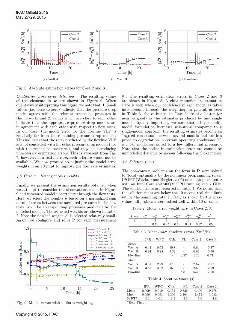
Fig. 8. Absolute estimation errors for Case 2 and 3.

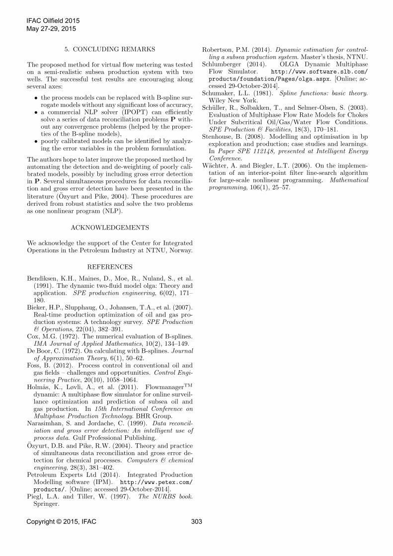
Qualitative gross error detection The resulting valuesof the elements in w are shown in Figure 9. Whenqualitatively interpreting this figure, we note that: 1. Smallvalues (i.e. close to zero) indicate that the pressure dropmodel agrees with the relevant reconciled pressures inthe network, and 2. values which are close to each otherindicate that the appropriate pressure drop models arein agreement with each other with respect to flow rates.In our case, the model error for the flowline VLP isrelatively far from the remaining pressure drop models.This indicates that the rates predicted by the flowline VLPare not consistent with the other pressure drop models (norwith the reconciled pressures), and may be introducingunnecessary estimation errors. This is apparent from Fig.7, however, in a real-life case, such a figure would not beavailable. We now proceed to adjusting the model errorweights in an attempt to improve the flow rate estimates.

4.5 Case 3 – Heterogeneous weights

Finally, we present the estimation results obtained whenwe attempt to consider the observations made in Figure9 and measured model uncertainty through the flow tests.Here, we select the weights ν based on a normalized sumnorm of errors between the measured pressures in the flowtests, and the corresponding pressures predicted by thematched models. The adjusted weights are shown in Table2. Note the flowline weight νfl is selected relatively small.Again, we configure and solve P for each measurement

0 5 10 15 20 25−1

−0.5

0

0.5

1

1.5

Time [h]

Model

error[bara]

IPR well A

IPR well B

WPC well A

WPC well B

Choke well A

Choke well B

Flowline VLP

Fig. 9. Model errors with uniform weighting.

yk. The resulting estimation errors in Cases 2 and 3are shown in Figure 8. A clear reduction in estimationerror is seen when our confidence in each model is takeninto account through the weighting. In general, as seenin Table 3, the estimates in Case 3 are also better (ornear as good) as the estimates produced by any singlemodel. Equally important, we note that using a multi-model formulation increases robustness compared to asingle-model approach; the resulting estimates become an”agreed consensus” between several models and are lessprone to degradation in certain operating conditions (cf.a choke model subjected to a low differential pressure).Note that the spikes in estimation error are caused byunmodelled dynamic behaviour following the choke moves.

4.6 Solution times

The non-convex problems on the form in P were solvedto (local) optimality by the nonlinear programming solverIPOPT (Wachter and Biegler, 2006) on a laptop computerwith an Intel Core i7-3740QM CPU running at 2.7 GHz.The solution times are reported in Table 4. We notice thatthe solution times are below the 10 second real-time limitset by the sampling rate. In fact, as shown by the max-values, all problems were solved well within 10 seconds.

Table 2. Model error weighting ν in Cases 2/3.

Case ν iprA ν ipr

B νwpcA νwpc

B νchkA νchk

B νfl

2 1 1 1 1 1 1 13 1 0.79 0.25 0.19 0.41 0.37 0.05

Table 3. Mean/max absolute errors (Sm3/h).

IPR WPC Chk. FL Case 2 Case 3

MeanWell A 0.42 0.53 10.8 - 0.64 0.17Well B 0.94 0.88 4.39 - 0.69 0.50Flowline - - - 3.27 1.20 0.71

MaxWell A 3.31 2.29 17.0 - 2.67 2.57Well B 3.87 3.82 16.3 - 2.60 2.99Flowline - - - 8.81 6.35 7.08

Table 4. Solution times (s).

IPR WPC Chk. FL Case 2 Case 3

Mean 0.009 0.010 0.151 0.326 0.496 0.478Max 0.096 0.093 1.396 2.104 2.472 3.032% RT* 0.1 0.1 1.5 3.3 5.0 4.8

*Real Time

IFAC Oilfield 2015May 27-29, 2015

Copyright © 2015, IFAC 302

5. CONCLUDING REMARKS

The proposed method for virtual flow metering was testedon a semi-realistic subsea production system with twowells. The successful test results are encouraging alongseveral axes:

• the process models can be replaced with B-spline sur-rogate models without any significant loss of accuracy,• a commercial NLP solver (IPOPT) can efficiently

solve a series of data reconciliation problems P with-out any convergence problems (helped by the proper-ties of the B-spline models),• poorly calibrated models can be identified by analyz-

ing the error variables in the problem formulation.

The authors hope to later improve the proposed method byautomating the detection and de-weighting of poorly cali-brated models, possibly by including gross error detectionin P. Several simultaneous procedures for data reconcilia-tion and gross error detection have been presented in theliterature (Ozyurt and Pike, 2004). These procedures arederived from robust statistics and solve the two problemsas one nonlinear program (NLP).

ACKNOWLEDGEMENTS

We acknowledge the support of the Center for IntegratedOperations in the Petroleum Industry at NTNU, Norway.

REFERENCES

Bendiksen, K.H., Maines, D., Moe, R., Nuland, S., et al.(1991). The dynamic two-fluid model olga: Theory andapplication. SPE production engineering, 6(02), 171–180.

Bieker, H.P., Slupphaug, O., Johansen, T.A., et al. (2007).Real-time production optimization of oil and gas pro-duction systems: A technology survey. SPE Production& Operations, 22(04), 382–391.

Cox, M.G. (1972). The numerical evaluation of B-splines.IMA Journal of Applied Mathematics, 10(2), 134–149.

De Boor, C. (1972). On calculating with B-splines. Journalof Approximation Theory, 6(1), 50–62.

Foss, B. (2012). Process control in conventional oil andgas fields – challenges and opportunities. Control Engi-neering Practice, 20(10), 1058–1064.

Holmas, K., Løvli, A., et al. (2011). FlowmanagerTM

dynamic: A multiphase flow simulator for online surveil-lance optimization and prediction of subsea oil andgas production. In 15th International Conference onMultiphase Production Technology. BHR Group.

Narasimhan, S. and Jordache, C. (1999). Data reconcil-iation and gross error detection: An intelligent use ofprocess data. Gulf Professional Publishing.

Ozyurt, D.B. and Pike, R.W. (2004). Theory and practiceof simultaneous data reconciliation and gross error de-tection for chemical processes. Computers & chemicalengineering, 28(3), 381–402.

Petroleum Experts Ltd (2014). Integrated ProductionModelling software (IPM). http://www.petex.com/products/. [Online; accessed 29-October-2014].

Piegl, L.A. and Tiller, W. (1997). The NURBS book.Springer.

Robertson, P.M. (2014). Dynamic estimation for control-ling a subsea production system. Master’s thesis, NTNU.

Schlumberger (2014). OLGA Dynamic MultiphaseFlow Simulator. http://www.software.slb.com/products/foundation/Pages/olga.aspx. [Online; ac-cessed 29-October-2014].

Schumaker, L.L. (1981). Spline functions: basic theory.Wiley New York.

Schuller, R., Solbakken, T., and Selmer-Olsen, S. (2003).Evaluation of Multiphase Flow Rate Models for ChokesUnder Subcritical Oil/Gas/Water Flow Conditions.SPE Production & Facilities, 18(3), 170–181.

Stenhouse, B. (2008). Modelling and optimisation in bpexploration and production; case studies and learnings.In Paper SPE 112148, presented at Intelligent EnergyConference.

Wachter, A. and Biegler, L.T. (2006). On the implemen-tation of an interior-point filter line-search algorithmfor large-scale nonlinear programming. Mathematicalprogramming, 106(1), 25–57.

IFAC Oilfield 2015May 27-29, 2015

Copyright © 2015, IFAC 303