World Bank Reprint Series: Number 409

Virnod Thornas

Diferences in Icomne andPoverty wt3tin Brazil

Reprinted with permission from World Development, vol. 15, no. 2 (1987), pp. 263-273, © 1987Pergamon Joumals Ltd.

Pub

lic D

iscl

osur

e A

utho

rized

Pub

lic D

iscl

osur

e A

utho

rized

Pub

lic D

iscl

osur

e A

utho

rized

Pub

lic D

iscl

osur

e A

utho

rized

Pub

lic D

iscl

osur

e A

utho

rized

Pub

lic D

iscl

osur

e A

utho

rized

Pub

lic D

iscl

osur

e A

utho

rized

Pub

lic D

iscl

osur

e A

utho

rized

Pub

lic D

iscl

osur

e A

utho

rized

Pub

lic D

iscl

osur

e A

utho

rized

Pub

lic D

iscl

osur

e A

utho

rized

Pub

lic D

iscl

osur

e A

utho

rized

World Development, Vol. 15, No. 2, pp. 263-273, 1987. 0305-750X187 $3.00 + 0.00Printed in Great Britain. @) 1987 Pergamon Journals Ltd.

Differences in Income and Poverty within Brazil

VINOD THOMASThe World Bank, Washington, DC

Summary. - Regional disparities in living standards within Brazil have received increasingattention in recent years. Drawing on the ENDEF consumption survey, this paper indicates that,although costs of living adjustments narrow spatial differences, large regional disparities remain,particularly upon comparing the Northeast and the Southeast. The application of price indicesreduces urban-rural variations more thlani regional differences, drastically narrowing theurban-rural gap in food consumption. Poverty is, nevertheless, much more concentrated in therural areas than in the urban areas, although regional differences in its incidence are morestriking than the urban-rural divergcrncies.

1. INTRODUCTION results of a 1974-75 nationwide householdexpenditure study - Estudo Nacional da Des-

Disparity in living standards across Brazil has pesa Familiar (ENDEF) -which divided the

been a matter of increasing concern. Rapid country into seven regions, as well as intoeconomic growth during the postwar years metropolitan, non-metropolitan urban, and ruralbrought benefits to lagging regions and areas, but areas (see FIBGE, 1977; 1978). Annual familyit is widely accepted that this growth process has expenditures on highly disaggregated consump-been very uneven. Large spatial inequalities in tion categories (including some 120 food items)living standards persist, as symbolized by the were surveyed. (Values of non-monetary compo-wealth in some areas (particularly the highly nents were imputed.) ENDEF reported familybtuilt-up urban centers of the Southeast), and the expenditures, the number of families, and familyvisible poverty in others. The Northeast region, sizes for nine expenditure classes. This permits aincluding nine of the country's 23 states (see rough estimation of per capita expenditures atbelow), accounts for the largest concentration of the mean and at partictular percentiles in thepoverty. According to some income surveys, the expenditure distribution. In addition to theNortheast region which has about 29% of Brazil's mean, the 40th percentile of each place is chosenpopulation also contains over one-half of the for comparison, since the latter represents acountry's poor, despite social and economic lower income group, avoids problems of dataprogress. inconsistency found at lower percentiles, and

Economic and social disparities between the presumably also involves consumption items thatNortheast and Center-Southeast may have some are relatively more comparable across locations.roots originally in the former's loss of ground in The expenditure data for income classes aresugar, while the latter gained from an expanding utilized to approximate continuous distributionscoffee market. Over time the divergences in the in the form of Lorenz curves. Against thewell-being may have resulted from recurrent expenditure distributions, estimated povertydroughts and unfavorable natural and institution- lines are used to determine the number of peopleal conditions in the Northeast, while economic defined as poor, and the extent to which incomespolicy favored the more dynamic Center- of the poor fall short of poverty thresholds. TheSoutheast. In the last two decades the Govern- poverty lines are calculated from the cost ofment has tried to implement policies intended to purchasing a basket of basic food items meetingpromote the development of the Northeast. some threshold nutritional "norms" and by theAccording to some estimates, the relative pos- actual non-food/food expenditure ratio whichition of this region has improved modestly in indicates the non-food "needs" of a given lowrecent years albeit from a low base, income group.

This paper provides a discussion of the differ- In comparing expenditure levels and construct-ences in incomes and poverty for a major regions ing poverty lines, nominal magnitudes are de-and areas within Brazil. The work draws on the flated by location-specific, cost-of-living indices,

263

264 W*RL[) DEVELOPMENT

whiclh show income and poverty differences more noted in comparing these with the remaining twoaccurately than otherwise, The overall price regions, that Region VI is all urban (Brasilia),index for any location relative to the national and that rural areas are excluded from Regionaverage is an average of food and non-food price VII.indices weighted by the expenditure shares of A limitation of the above approach lies in itsthese categories. The food price index is esti- use of national expenditure weights rather thanmated directly from the ENDEF data on food of location-specific ones. An alternative methodexpen(ditures and quantities consumed. A non- would be to express at niational prices the cost offood price index, on the other hand, is approxi- baskets of food consumed in each place. In thismated froim the expenditure data, since no procedure, corresponding to Paasche priceestimates of quantitiesare available. Considering index, expenditure weights of individual loca-the tentative natuire of this index, some sensitiv- tions rather than the national averages would beity tests are performed and a low and upper used.3 Clearly, least-cost options available inbound provided for these measures. individual locations should be reflected, which

would best be done by considering price differ-ences of low-cost location-specific food baskets

2. VARIATIONS IN LIVING COSTS rather than a nationwide average basket. On theAMONG LOCATIONS other hand, in indicating overall spatial differ-

enices in food prices, it mav be logical to first(a}) Food prices compare onie national composite food basket.

The Laspeyre index is utilized here to measureT'he prices of over 12i) individual food items price differences of food and to produce regional

have beeni calculated for the various regions and comparisons of food consumption. In the con-areas for 1974-75 (see Ilicks and Vetter, 1981; struction of poverty levels, on the other hand, theKniiglht t til., 1979: Malard Mavyer, 1981; Prado cost is compared among baskets of food, main-and Macedo, 1980; Williamson, 1981). In one set taining their location-specific proportions. Oneof estimates, spatial price inidices have been price index based on location-specific con-cilClahited for a basket of food items in their sumption pattern is given in the second column ofnational average proportions, wlhich corresponds Table 1. This index, constructed from data into a Laspeyre price index.2 First, a price index Knight et al. (1979), shows the price differencesfor each food item has been calculated, with the of a food basket consumed at the 20th percentilenational price which has beeni obtained bv of the expenditure distribution, maintaining eachweighting each location's price by the location's location's consumption pattern. The large urban-quantity weight in the national total - as the rural price differences according to this indexbase. These price indices have then been weight- reflect and ability of the poor in rural areas toed across various items using their respective meet nutritional needs at relatively low costs, asexpenditure shares at the national level. The long as their own actual consumption patternsresulting price indiex for any location reflects the are maintained.difference in price in that location from the Food prices increase going from rural to urbannational price (assumed to be 100) of a nationally areas and from the mnore rural to the moreconsumed average basket of food. urbanized regions. Regions I and 11, as well as

A recent study (Thomas, 1982) set out the VI, where the percentage of urban population isprice indices for 10 major subgroups of food high, consistently show a price level well aboveitems and for a composite food bundle, indicating the national average. Regions IV and V. as wellsignificaTnt price differences. Comparing metro- as Region III, are less urbanized and face belowpolitan Sao Paulo, the largest lirban center, with national average prices.its adjacent rural areas (Region II), an uirban- The index based on the consumption pattern ofrural price difference of 14% is observed. Be- the 20th percentile is the basis for the povertytween metropolitan Sao Paulo and an even more measure presented later. In the case of Laspeyrerural area in the Northeast (Region V), a price or Paasche price indices used to deflate incomes,difference of 35'%f is noted, weighting by quantities consumed of individual

Regional differences are a part of the latter items and by expenditures across items is appro-result. The average price in the Sao Paulo state priate. For use in estimating the number of poor,(Region II) is 16' higher than in the Northeast, or for measuring incomes needed to eliminateas summarized in Table 1. The first two of the poverty, the weighting of costs or prices mustfirst five regions, which contain Rio de Janeiro take into account the number of people affectedand Sao Paulo, respectively, face higher food by the relevant costs or prices4 as will be done inprices than Regions III, IV and V. It shoulcd be this paper.

IO'ONIF. AND POVERTY IN BRAZIL 265

Table 1. Estimated food, non-food anZd overall price indices for regionis and areas: Brazil, 1974-75

Food Non-food Overall*

B. Location- National 20thA. Average specific Based on 40th average Percentile

national basket of percentile food and food andbasket 20th percentile expendituret non-food non-food

Regions

Region I 1i1 126 175 151 162

Region II 116 123 148 138 141

Region III 96 95+ 94 95 94Region IV 96 82 87 90 85Region V 10( 83 n.a. n.a. n.a.Region VI Brasilia 121 140 146-156 137-146 1-4-152Region VII 118 78 110 113 100

Areas

Metropolitan n.a 131 152-161§ n.a. 145-154§- Rio de Janeiro (115) (135) (182-194) (159-165) (166-179)- Sao Paulo (124) (146) (196-207)§ (171-179) (179-193)§- Porto Alegre (108) (138) (150-158) (135-144) (146-153)- Belo Horizonte (112) (11()) (128-133) (122-127) (122-127)

- Salvador (120) (137) (128-133) (125-130) (131-134)

Other urban n.a. 93 1()5 n.a. 100

Rural n.a. 78t n.a. n.a. n.a.

National average 1(( 10(0( 100 () 1(00

*Using national weights of food and non-food expenditures.tThe lower figures assume that 1(0% of the higher non-food expenditures in metropolitan areas are

directly due to the consumption of items not readily available in other places.

tAn exceptionally large non-monetary component for rural areas renders these price indicesquestionable.§It may be advisable to omit Sao Paulo from these comparisons for reasons given in the text.n.a. - Not available, due to inconsistencies in the data.

(b) Nont-food prices the other, because non-food prices vary. Differ-ence in incomes along with an income elasticity

The ENDEF data for non-food do not permit of demand, and difference in prices along with a

derivation of price indices since no estimates of price elasticity of demand, together explain the

the quantities consumed are given. No other non-food quantity variation. To obtain a price

independent estimates of non-food prices, even ratio, with the national average as base, we write

for the major items, are available for the ENDEF the known expenditure ratio between any loca-

regions and areas. Therefore, spatial price ratios tion j and a hypothetical national average (calcu-

have been approximated from data on expendi- lated) i as equal to the ratio between price in j

ture differenitials as discussed below (see also and the price in tn (100) times the quantity ratio.

Medeiros, 1977). The latter quantity ratio is related to the income

A given expediture difference between two and price differences between j and in and the

locations may be in extreme cases entirely due to income and price elasticities at m. This allows us

a price difference or entirely due to a quantity to solve for the price in j as a proportion of the

difference. It has been assumed that onlv part of price in in, 100.

the difference is due to a price difference, the rest This approach identifies the change in quantity

being due to a quantity difference. The non-food consumed by someone who experiences a change

quantity difference is postulated to arise, on the in income and price in going from in to j, leaving

one hand, because money incomes vary, and on the remaining difference as the price variation.

266 WORLD DlVIEL I.( ;PN NT

Tlhe estimated quantity clhange is dictated bv the While the problem posed by qualitv differ-elasticities measured in the h) potheteicil average ences is by no means removed, a better compari-location (i.e., usinlg data for all locations). I'his son of the price of a non-food basket is possiblemethod will not fully idenitify differenices in the at the 40tth percentile than at the mean. PricesquaLntity consumetd in a particular place that arise vary systematically, exceeding 100 in the urbzand3ue to location-specific ineeds, for instance, the and relatively more urbanized regions, and fallpart of uarban people's higher consunmptioni the below 100 in the more rural locations with almostlarger quantities conisumned of transportatioil a one-to-one correspondence between the priceclothing, and safety devices arising pturely from index and the degree of urbanization, going fromliving in the city, will not be reflected. Suclh metropolitan Sao Paulo, Brasilia, and metropoli-quantity differences, bevonid those in the "aver- tan Rio de Janeiro to the rural areas of Espiritoage" location, will instead become part of the Santo, Minas (jerais, anid the Northeast. Amongprice differences. This feature is reasonable as the few metropolitan areas and small towns in thelonig as these quantity differences do not enhance couuntryside, a price difference of roughly 50% iswelfare (e.g.. urban dlwellers are n1ot better off estimated (Table 1).because they travel inore). If, on the contrary, Considering the limitations of the non-foodsuch differences contribute to welfare, the price price estimates presented, we tried to directlyindex for urbanl areas as calculated in this paper assemble price estimates for major non-foodwill be biased upwards. To correct for this categories. The 1970 Demographic Censu.s pro-possibilitv, in one set of calculations it has been vides information on rents paid by nine rentassunmed that 10)%, of thie expenditure difference groups in 126 urbani municipalities located in thein the metropolitanf areas is independent of price states of Rio de Janeiro, Sao Paulo, Minasvariations, antd this 10% -( in addition to the (erais, Espirito Santo, Parana, Santa Catarina,result of the above calculations - is fully due to Rio (Grande de Sul and Goias, and Brasilia. Forreal consumption differences (see Table I). metropolitan areas within these states, several

Price and income clasticities of demand for municipalities were aggregated. It was possible tonon-food items could not be calculated, since no separate out the rent paid for four-room housesdata on the quaintities of non-food items con- serviced by water and sewer networks withinsumed wer e available. It has been possible, these rent groups. From this information, medianhowever, to tuse estimated elasticities for food rents were calculated for what may roughly bealong with average budget shares of food and considered comparable housing in each of thenon-food goods to derive non-food elasticities, municipalities. Restults for selected metropolitanapplying the Slutsky eqLuations as explained in an and other urban areas are given in Table 2.earlier paper (see Thomas, 1980a; 198t)b). Oneimprovement in this study is that comparisons atthe 40th percentile of the nominal expenditure T'able 2. Miedian renits for comparabledis,tribUtioii are also made, in addition to those at louisiig -1970the mean.

At the 40th percentile, income and price Price indexelasticities of demand for food have been calcu-lated from ENDEF data to be (1.86 and -1.2,respectively. To transform these food elasticities Metropolitan areasinto non-food elasticities, national average Rio de Janeiro 137budget shares of food and non-food were calcu- Sao Paulo 126lated to be 0.4 and 0.6, respectivelv. Also, the Porto Alegre 122lae oCuritiba 1(15demand elasticities of income and price for food Belo Horizonte 105at the mean have been calculated to be 0.54 and Brasilia 146-0.38.

The use of national budget shares and national Smaller cities atnd townselasticities is analogous to the use of national Cainpinas 94weights to obtain regional prices applying Las- Ribeiro Preto 8X)peyre indices in the case of food.5 Budget shares Florianopolis 49are clearly non-uniform across regions, and Ouro Preto 43significant urban-rural differences in price andincome elasticities are bound to exist. To provide Average* 10(an idea of the sensitivity of the results to varyingbudget shares and elasticities, a number of Source: Calculated from the 1970alternative estimates were tried, which did not Demographic Census.affect the results significantly. *Average for 126 municipalities.

INC'OME AND Pl(T'OV l'Y IN BRAZIL. 267

(c) Overallprices mean, urban areas in general show greater foodintake. When the 40th percentile is considered,

Overall prices have been calculated using the however, the position of the rural people im-

non-food index for the 40th percentile, and using proves even further relative to urbanites. In some

the food price index at the mean for the low-cost instances, rural consumption of food in real

diet. As seen in Table 1, the more affluent and terms at the 40th percentile is even higher than

urbanizedi locations clearly display higher price that in the metropolitan areas (Solarzano, 1981).

levels. Region II's prices are roughly 50%) higher Furthermore, it is shown in Campino (1980) and

than in Regioins III and IV. Compared to the T'homas (1982) that w-ile rural areas among high

national average, the metropolitani area's prices income regions such as Regions JI and III, with

are about 50)% higher, while the rural areas' the moderately wealthy but largely rural Region

prices are probably about 259%, lower.' Prices in IV, achieve the highest intake of calories both in

the metropolitan areas are significantly higher absolute and relative numnbers in comparison to

than in the rest of the country. Living costs in requirements, other high income regions, which

metropolitan Rio and Sao Paulo appear to be are the most urbanized, such as Regions I and

some 60%!/,, above the national average. It should VI, perform worse. The nation's poorest region,

be noted, however that metropolitan Sao Paulo's the Northeast. and particularly its metropolitan

non-food expenditure estimates are so far above areas, remain worst off in nutritional terms,

the rest that the cost of living indices derived indicating a spatial dimension for targeting nutri-

using the national -average" income and price tional policy.elasticities may not be satisfactory for this loca-tion. The non-metropolitanl urban areas' (i.e., (b) Nont-food consumlption

small towns') prices correspond roughlv to tienational average. Nominal expenses on non-food items vary far

The contribution t(o true living costs oi urban more than on food. The non-food price index

amenities or disamenities, urban public goo(ds also has a larger spread than the food price

and services, andi other government services are index.7 Consequently, real expense differences

not fully accounted for in the presenit calcula- are diminished more in the case of non-food than

tions. Some factors, such as the availability of food. Nevertlheless, larger spatial divergenciespublic services, widen the true urban-rural price remain in non-food consumption than in food,

differences, while others, such as pollution, indicating that the former are the more signifi-conaestion, and crime narrow the true differ- cant sources of the overall differences.ences. One approachi toi capture these effects The more urbanized regions and areas achieve

might be to compare the monev wage differen- a much higher consumption of non-food categor-

tials across locations for labor with similar ies than the rest of the country. People in

education anid/or skills, assuming that significant Regions I, II and VI, with the largest rnetropoli-

real wage differenltiails for comparable labor are tan centers (Rio, Sao Paulo, ind Brasiiia, respec-

unlikely to persist. tively) consume, on average, more non-fooditems than the national average. The moderatelyurbantized Region III also consumes a little over

3. SPATIAL INE JUALITYO F the average, while the largely rural NortheastEXPENDITURE (Region V) and Region IV fall below the

average. The Northeast consumes less than half(a) Food c-onIsIu tizon of Regions I, 11 and VI.

The comparison of urban and rural areas

As shown in Table 3, while the gap in food shows that non-food consumption varies positive-intake is narrowed somnewhat by using real rather ly with income andi the degree of urbanization.

than nominal consunmption, significaint disparities Contrary to the case of food, non-food consump-

remain among regionis (see also Knight et al., tion in the metropolitan areas exceeds that in the

1979; Lluch, t981t; Pfeffermiiann an(i Webb, 1979; urban areas significantly at the 40th percentile.

Prado and Macedo, 1980). Food consumption is The estimated gap is 18%. At the mean, con-

the lowest in the Northeast region, which also has sumption in metropolitan areas is higher than the

the lowest income levels suggesting the import- national average by a range of roughly 14% to

ance inter a/lia of more rapi(d growth to alleviate 44%X0 (Table 3).food inadequacy.

The large urban-rural differences in nonminalterms are also sharply reduced when comparisons (c) Total consumption

are made in real terms. Nevertlheless, at the Compared to total nominal expenditure, real

268 WORLD DEVELOPMENTI-

Table 3. Mean annutal per capita expenditures for regiotis and areas: Brazil, 1974-75

Food Non-food Total

Nominal Real' Nominal Realt Nominal Real:

Regions

Region I§ 1,895 1,707 5,10() 2,914 6,995 4,621(2,132) (1,921) (5,737) (3,278) (7,869) (5,199)

Region IT 1,674 1,443 4,419 2,985 6,093 4,428Region 111 1,542 1,606 2,746 2,921 4,288 4,527Region IV 1,323 1,378 2,285 2,626 3,609 4,004Region V 1,029 1,029 1,234 1,26011 2,357 2,28911Region VII 1,681 1,425 3,163 2,875 4,844 4,30)0

Selected cities$

Porto Alegre 2.093 1,937 6,207 3,928-4,138 8,300 5,76.5-6,075Sao Paulo** 2,228 1,797 7,399 3,574-3,775 9,627 5,371-5,572Rio de Janeiro 2,219 1,930 6,381 3,289-3,506 8,601 5,219-5,436Region VI-Brasilia 1,711 1,414 5,707 3,658-3,909 7,418 5,072-5,323Salvador 1,599 1,333 4,857 3,652-3,795 6,456 4,885-5,128Belo Horizonte 1,611 1,438 5,143 3,867-4,018 6,755 5,305-5,456

Natiotial averaige 1,441 1,441 2,880 2,880 4,321 4,321

Source: Calculations based on FIBGE (1978) and Table 1.*Dividing nominal expenditures by the food price index in the first column of Table 1.tDividing nominal expenditures by the non-food price index in Table 1.t('olumn 2 plus column 4.§There is some ambiguity about the appropriate average family size to be used for this region,giving two alternative per capita estimates, the first assuming average family size of 4.5, andthe second 4.An approximation using monetary expenses alone was made since the non-monetary

component for the rural areas contained inconsistencies.¶The higher values for real non-food expenditures assume the lower non-food price indices inTable 1.**Perhaps Sao Paulo should be excluded as mentioned earlier.

consumptioni displays a smaller spatial variance, 4. DIFFERENCES IN POVERTYwith a major part of the remaining differencearisina from disparities in non-food con3umption, (a) Food costsparticularly if lower income groups arecompared. At the 40th percentile, the metropoli- Three poverty levels have been calculatedtan urban-rural variation is lessened consider- (Prado and Macedo, 1980) based on low costablv, but is by no means eliminated, At the food consumption baskets. These poverty linesmeani, larger urban-rural differences persist. differ from each other in minimum nutritionalAmong the metropolitan areas considered in requirements (alternatively, Campino, 1980 andTable 3, total consumption in real terms exceeds FAO/WHO, 1973), food composition, and foodthe national average by a range of 13%X0 to 41°%. prices. The arbitrariness and shortcoming of

These remaining estimated differences in real utilizing such estimates of nutritional require-consumption do not necessarily imply that ments are fully recognized, but they should notcomparable labor earns significantly different hurt this analysis of regional differences. One ofreal wages across regions in Brazil. Comparisons the poverty lines representing a "medium" levelat the mean or even at the 40th percentile in each is reported here. Food price differences reflectedlocation, as presented in this paper, are in- in this and other baskets are different from theadequate. In order to evaluate this issue, some mean food price index in Section 2 for threeadjustment for skill levels or at least for edu- reasons: first, the baskets considered are differ-cational levels of the population compared will ent from the mean; second, the prices at thebe necessary. lower income percentile are also different from

iN(O()MIE: AND POVERTY IN BRAZIL, 269

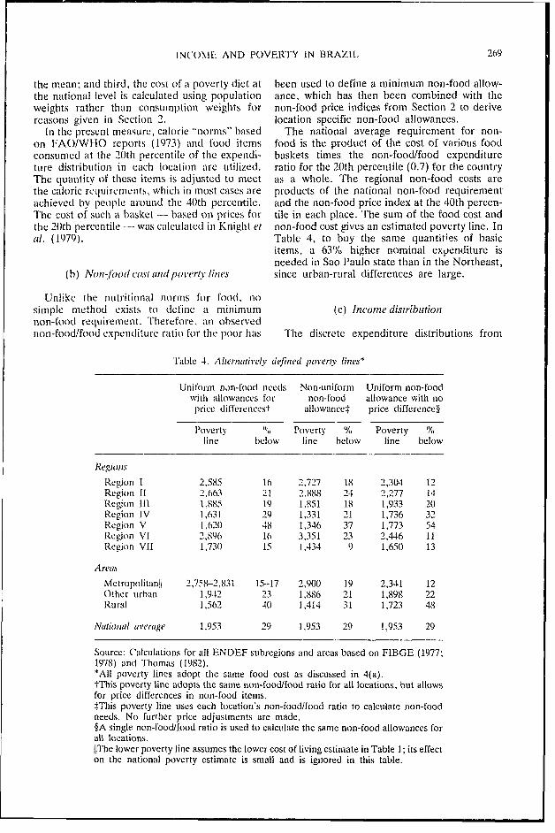
the m,ean; and third, the cost of a poverty diet at been used to define a minimum non-food allow-

the national level is calculated using population ance, whlich has then been combined with the

weights rather than consumption weights for non-food price indices from Section 2 to derive

reasons given in Section 2. location specific non-food allowances.In the present measure, caloric "norms" based The national average requirement for non-

on FA0/Wo10 reports (1973) and food items food is the product of the cost of various foodconsumed at the 20th percentile of the expendi- baskets times the non-food/food expenditure

ture distribution in each location are utilized. ratio for the 20th percentile (0.7) for the country

The quantity of these items is adjusted to meet as a whole. The regional non-food costs arethe caloric requiremnlits, which in most cases are products of the national non-food requirement

achieved by people around the 40th percenrtile. and the non-food price index at the 40th percen-The cost of such a basket - based otn pr-ices for tile in each place. The sum of the food cost and

the 20th percentile - was calculated in Knight et non-food cost gives an estimated poverty line. Intcl. (1979). Table 4, to buy the same quantities of basic

items, a 63% higher nominal expenditure isneeded in Sao Paulo state than in the Northeast,

(b) Noni-food cost and poverty lines since urban-rural differences are large.

Unllike the nutritional norms for food, nosimple method exists to (lefine a minimum (c) Income distribtitionznon-food reqtuirement. Therefore, an observednon-food/foo(d expenditure ratio for the poor has The discrete expenditure distributions from

Iable 4. Alternatively defined povertv !ines*

Uniiform non-food needs Non-uniform Uniform non-foodwith allowances for non-food allowance with noprice differencest allowancet price difference§

Poverty " Poverty % Poverty '%line below line below line below

Regiotns

Region 1 2.585 16 2,727 18 2,304 12Region 11 2.663 21 2,888 24 2,277 14Region 111 1.885 19 1,851 18 1,933 2(0Region IV 1,631 29 1,331 21 1,736 32Region V 1,620 48 1,346 37 1,773 54Region VI 2,896 16 3,351 23 2,446 11Region VII 1,730 15 1,434 9 1,650 13

Area.s

Metropolitan!i 2,758-2,831 15-17 2,900 19 2,341 12Other urban 1,942 23 1,886 21 1,898 22Rural 1,562 4(0 1,414 31 1,723 48

National average 1,953 29 1,953 29 1,953 29

Source: Calculations for all ENDEF subregions and areas based on FIBGE (1977;1978) and Thomas (1982).*AII poverty lines adopt the same food cost as discussed in 4(a).tThis poverty line adopts the same non-food/food ratio for all locations, but allowsfor price differences in non-food items.:This poverty line uses each location's non-food/food ratio to calculate non-foodneeds. No further price adjustments are made.§A single non-food/food ratio is used to calculate the same non-food allowances forall locations.IlThe lower poverty line assumes the lower cost of living estirmate in Table 1; its effecton the national poverty estimate is small and is ignored in this table.

270 WORl.l) [)FLVPI .()PMFNTI

ENDEF were used to fit a Lorenz curve based on of povertv (Thomas, 1982). SCecond, the use ofthe method suggested in Kakwani and Podder the noni-foo(d price index is likelv to liave giveni a(1976). Discrepancies in the data for extreme more accurate presentation of thle poverty profilevalues (particularly the first two dieciles andi the than other measures, Fwo alternative methodslast) affectedl the resuilts in several cases, and a could have beent, first, to assume thiat all non-geometric approximation of an ex pend iti.rc food expendliture differences are price (liffer-distribution in the neighborhood of the povertv clnces. and second, to assurme that all n1on1-foo(dline had to be relied upon instead, vielding exlplediturc (differences are real (quantitv) (diffcr-estimates of the percentage of poor people. In ences. Under the first assumption, larger thanthe neighborhood of this estimate a Lorenz curve necessary urban-rural differelnces in Poverty lineswas also geometrically fitted to calculate incomes woul(d be aidopted. resulting in smaller spatialof the poor. Results are given in Thomas (1982). differenices in the incidence of poverty than

The ENDEF expenditure survey-based income fountd in this paper. Ulnider the second assump-distribution measures, which are developedi in tion, a uniform non-food allowance would blethis study, show a lesser concentration of income used with the povertv line restulting in widlercomparedl to previous demographic census-based spatial differences than suggestedi here.estimates (see Fonseca, 1981; Lluch, 1981; Pfef- Both these :alternatives hive been tried. infermann and Webb, 1979; rhomas, 1982 for both cases assuming the same foo(d expeindliturediscussions). One reason is that the expen(diture as shown in Table 4. The first columtn results aredata reflect permanent income better than the based on the "mediuLn" poverty definition. Theincome data, which often understate income-in- second columni reports the povertv estimates thatkind and secondary incomes. The expenidliture- would result if the actual noll-food/food ratios inbased distribution also captures the incomiie of each location were assumed necessary to meetlower income groups better, thereby showing a nlinimum needs. Thus, the full differeclce inlower concentration than the income-based dis- observedl expenditures on non-food is assumlledi totribution. Furthermore, ENDEF excludes those be due to price differenices, wlhichi in realitywith significant expendliture, thereby understat- w.nild he an exaggeration. Consequently. pover-ing the true degree of concentration. Perhiaps for tv differences woulLd unwderstate true dlifferences.these reasons, ENDEF also shows a consistent Thle third ColumnII assumes that the samie non-and significantlv lower inconme concenitraitioni in food allowance calculated at the national level isrural areas than in urban zoiles, more so thaln sufficient in all regions. This presumes no spatialwhat appears in income-based estimates. price dlifferences, an1d as a resuilt, exaggerates the

variation il lpovertV.

A se:ond mlezasure of po(,erty takes into(d) IPovertY ineasure's account botlh thle percentage of people whio are

poor (as above) and(i thie extenlt of their poverty.The "medeiunfi definition imnplie. that about Ihe Sen Index given below (I) considers lbotl

29l"o of the naitioin's population are poor (Table these components.4), which compares with in estimate of 271't, b)vPfeffermannziii .and Webb (1979). However, a nmore N,, Y - Y,, (I - (,)interesting findiing for policvniakers is that the j = (I)distribution of the poor is verv uneven across N Ylregions, with great concentrations in the North-east and rurail areas. About 14 millioll People in Where: iVN, is theC nulllber of poor: N' is thie totalthe Northeast are considered poor, wlhich is alsoi population; Y is the poverty line: Y',, is theabout the size of the rural population tdefiniel as average inconme (expenditure) of thle poor; andpoor. Some arbitrariness in the clhoice and U,, is the (Gini coetficient of consumiiption of theapplications of poverv lines is evident %lhen poor. If all poor have the same in1comIle (i.e.. G,,comparing results based on alternative = )), the in(lex is the product of the perceniapethresholds. If a "low definition of poverty vere of poor people times the proportion of incoilmeadopted. obviouslv mnuchi loweer numbers would short of the poverty line. If the distribution ofbe defined as poor -23"%O to 24%', according to income amiong the poor is also important. (I -SolorZano (1981) and Thomnas (1982). U,1) weights Y such that a worse distribution

In spite of the tentative nature of the nonI-food results in a larger poverty index.price inldex in this paper, two results are impor- If the distribution of income among, the poor istant and robust. First, the relative positionXs of ignored and the poverty gap (Y* - Y;,) islocations in the incidence of povertv would he expressed as a fraction of the average incoime ofbroadly maintained undler alternative definitions location Y (rather than P'), the resulting index

INCO()ME AND) POVEIRT lY IN BRAZIL 271

wouldl indicate the percentage of a location's would go to the poor. IHowever, the spatialexisting total incone that is nee(letto ble directed distribution of this needed increase is veryto the poor to enable themii to cross the poverty uneven. In the case of the Northeast, thelevel. This in(dex ', pro1)osCLI in Thornas (1980b). required increase is 10)% compared to that ofis given below: tabout 1.6%X, in the state of Sao Paulo. For the

rural areas i1s a whole more than 10% increase isN, Y'* -Yt, 2 needed as compared to abouit 2'% in the metro-

I N (2) politan areas.

where V is the average income of the region. 5. CONCLUSIONTable 5 presents estinmates of equLations ( 1) and

(2) based on the "mediumt" poverty line. Brotad Estimated cost of living varies significantlydifferetnces in these indices are similar to tthe ones within Brazil, ranging from roughly 150 or moregiven by the percentage poor, but some of the in the cities of Sa) Paulo, Rio dce Janeiro, andurban-rural differences are reduced due to better Brasilia - comipared to a national avcraverural incomle distributions implied in ENDEF. (weighted) of 100 - to about 100 in the majoritySome of the regional differences are augmetnted, of small towns, and 90 and less in the rural areas.also because sonme of the poorer regions have The application of these price indices, in additionworse income distributions. to the inclusion of non-monetary components,

Equation (2) indicates that in order to enable niarrows estimated spatial divergencies in realeveryone to have inconme equal to or above a exnr(littires, particularly in the case of a lower"medium" povertv line, over a 5%() increase in in'come group (the 40th percentile) and uponannual national income is neelded (over the comparing urban and rural areas within regions.actual increase in 1974-75). All of this increase In spite of these adjustments, however, large

regionial differences remain.When comparing urban and rural locations,

Table 5. Povert' measusres real expenditures on food especially appear to beevene(d out. In fact, the poor in many rural areas

"Medium*" poverty line seeti to achieve comparable or better nutritionalintake than their urban counterparts. Across

Poverty Income regions, on the other hand, food intake and'to below index* deficiency %t nutritional levels vary sustantially reflecting the

large regional differences in real incomes.Regions The major proportion of the urban-rural dif-

Region I 16 IU 2.4 ferences in real terms arises from non-foodRegion IS 21 8 16 consumption, even though the non-food priceRegion [II 19 8 1.9 index in this paper may have overstated the trueRegion IV 29 18 4.8 urban-rural price differences. In spite of aRegion V 48 26 1MO.) markedly higher non-tood/food relative price inRegion VI 16 7 1.2 urban areas compared to rural zones, urbanRegion VII 15 13 2.8 dwellers consume relatively more non-food items

than rural people. Higher urban incomes andAreas higher income elasticities for non-food items

Metropolitanf 15-17 9-10 1.9-2.1 relative to food are probably the main reasons forOther urban 23 14 4.5 this phenomenon. But the question also asks whyRural 40 19 10.1 urban dwellers with equal or higher real incomes,

in some cases, seem to consume less food (andmore non-food) than their rural counterparts.Part of the explanation may lie in quality

Source: Calculations for all ENDEF subregions and differences of the items consumed. Urban con-areas based on FIBGE (1977; 1978) and Thomas sumption of certain non-food categories whicl(1S2 )I .i equation (1)ultipliedby are simply not available in rural areas may be

tEquation (2) multiplied by 100 another part of the explanation. Furthermore,t:he lower estimates for metropolitan areas assun.e inadequate availability of public goods and ser-the lower price indicos in Table 1; their effect on the vices in rural areas represents an importantnational poverty profile is small, and is therefore source of disparity, which is not addressedignored in this table. adequately by expenditure measures.

272 WORDI) DEVELOPME NT

A conservative definitioin of poverty at the This paper has not primarily concerned thenational aggregate level indicates that if a 5'%,,. policy implications of regional and urban-ruralincrease in annual national income above thc income differenetials. It has, however, tried tolevels existing in 1974-75 were entirely directed highlight the importance of niciusuring cost oftowards the poor, everyone would have been at living (differences, and thus Obtaining more accur-or above the poverty line The more interesting ate measures of income aned poverty levels. f oroutcome of the poverty measures undoubtedly providing a fuller basis for policy. clearly thepoints out that considerably more poverty exists tren(ds in regional divergences over time shouldin the nation's rural areas than in urban areas, also be studied. Avenues for policy evaluationFor instance, a poverty index for the nation's wouldl incluide several questiolns: Hlow much ofrural areas is al)pro::inlatelv 27%' 9" higher than the the differences have been and might be broughtnational average, while that of the nmetropolitatni down by rapid economic growth'? What has beenareas is nearly 4t%, below national average. the effectiveness of regional policies and effortsCompared to such urban-rural differences, how- to increase the efficiency of use of regionalever, some regional differences, particUlarly be- resoturces? TIo what extent can policies to im-tween the Northeast and the Southeast, are more prove the mobility of resources reduce dlispari-striking. In particular, while a poverty index for ties?Sao Paulo state is roughly 50",, below thenational average, 'hat for the Northeast is 70%higher than this . -erage,

NOTEiS

1. The regions arc: I - the state of Rio de Janeiro: 4. 'I'o take an example, ift 8t"', of the nationalII - the state ol' Salo Paulo: III Parana, Santla population who live in location I face PI and 2i"., InC(atarina, Rio (Orand do Sul; I - Espirito Santo. location 2 face Pr tor ai food basket, the national

Minas Cierais: V- the Northeaist, i.e. Maranhao, average income needed to purchase thia.t basket wvouldPiaui, ('ea.ra, Rio Cirande (do Norte, Paraiba, Pernam- be the average ot'f / and ', Nveighlted by the respectivebuco, Alagoas, Sergipe antd B3ahia; V'T BIrasilia; VII population shares. ll.8 and 0.2. Weiglting biv the

Rondonia, Acre. Roraima, Para, Amrapa. (iias, quantities consuiiC(ei in the two locations would beMato (irosso. inappropriate. I'hereto're, in poverty measures, re-

.gion1al average aniid national average p)overtv leveis are2. i.e .,. constructedi 1y weighting asverage location-speciflic

poverty lines, usinyg populationi wNeights.

( ' 'I'he alternative. analogous to Paasche's, would bleX j, to compare the national average with each location as a

1P , . or. X _,I'.s base. 'I'his procedure was applied to the cases of a few

', l specific income and price elasticities for lood andbudget shazes for foo(d and non-Food: the resultinginttr-locaitiorn differences are not verv diiff'rent from

where P1 and X' are prices and quantities. respeettivels. those reported in this paper.for commoidity i going from I to n in anv location j.compared to a national average location in. 6. Urban-rural comparisons are approximations for

the Northeast andl the nation as a whole, diue to data3. i.e .. problems in the rural Northeast.

7. Price indices for non-foodJ are based on totalI-,'l" \ \P expenses at the meain an(d only ronetary expenses tit

f [t (P p the 4t)th percentile. TIable 3 summarizes the mnainresults for the mean, wvhile Solorzano (1981) andThomas (1982) provide details for both types of' indices.

INC( ()M AND) )VVER'iT'Y IN BRAZIL 273

RIEF:[ LRENCES

Bhalla. Surjit S., '"Mtasuremlent oi poverty Issues Brazil," Draft (Washington, DC: 'I'he World Bank,

antd incihod'." Monograph (WMshington, DC: 'T'he May 1981).World( Bank, 2) January 1980). Malard Mayer, Maria Martha, "Comparacoes entre os

Campino. Antonio C. C., "('ustos de programras de Niveis de Precos nas Areas Metirapolitanc.- Abrangi-

suplementaca(o alimentar no mieio urbano," Revista das Pelu Sistema Naci6nal de Indices de Precos ao

lonomica dlo ioVrde.ste, v'ol. I, No. 2 (April/June C'onsumidor" (Rio de Janeiro: DESIP, FIBGE,

198). August 1981).

FAO/WI10), Energy antd P'rotein Requirements: Report Medeiros, Paulo de l'arso, "Diferencas (icogralicas no

/ fa Joint F.A04W10 Ald Hoc' Erpert (Comnmnittee, Custo de Vida," Rev. Bras. Ecotn., Vol. 31, No. 2

FAo) Nutrition Meeting Report Series No. 9, WHO (1977).Technical Report Series No. 522 (Rome: FAO/ Pfeffermann, Ciuy P., and Richard Webhl, "'The

WHR), 1973). distribtution of income in Brazil," World Bank Staff

Fonscca, Marcos (G. da, "Radiogralia da D)istribuicao Workintg Paper No. 356 (Washington, DC: The

pessoal de renda no Brasil: Ulma zdesagregacao dos World Banik, September 1979).

indices de (iini," Estudos Eco,nmicumw , Vol. 2, No. I Prado, EIcuterio F. S., and Roberto B. M. Macedo,

(January/March 198!). Dimetnsao Regionzal da Pobreza: Utn Reexamne do

Fundacao lnstituto lirasileiro de (icografia e Estatisti- Problemc: do Nordeste Brasileiro, A FIPE Research

ca (FBIBGFi), Eistu(io Nacional zia D)espesa Familiar Project, Final Report (Sao Paulo: FIPE, April 1980).

( N -)1 ' ), (Conswnno Alimnentar: -lntropoincetria, Sen, A. K., "'Poverty: An ordinal approach to measure-

Dados IPrelitninares 7 volumes (Riot de Janeiro, 1977 ment," Economnetrica, Vol. 44 (March 1976).

and 1978). Solorzano, C'uadra Eduardo, "Difererncas Espaciais de

FIBGjE, EINt)EF, l)epa.% dals Famnilias, D)ados Pre- Nutricuo, Renda e Probreza no Brasil," Mimeo (Sao

liminares. 7 volum%es (Rio de Janeiro. 1978). Paulo: University of Sao Paulo, 1981).

flicks, James F, Jr., and David Mv1. Vetter, "Identifving T hhomas, Vinod, "Spatial differences in the cost of

the urban plan in Brazil." Draft Version, World living," Journial of Urbatn Economics, Vol. 8 ( 1980a).

Bank Research Proposal No. 672-37 (Rio de Ihomas, Vinod, "Spatial differences in poverty: The

Janeiro, Brazil, Julyv 1981). case of Peru," Journal of Development Economics,

Kakwani, N. E.. ain( N. Podder, "Eflicient estimates of Vol. 7 (1980b).

the L.orenz curve and associated inequality measure Thomas, Vinocd, "Differences in income, nutrition and

from grouped observations," h ontometrica, Vol. 44. poverty within Brazil," Staff Workinig Paper No. 505

No. 1 (1970). (Washington, DC: The World Bank, February

Knight, P. 1., R. Mloran, C. l luch. O). Mahar and F. 1982).Swett. Brazil: Hlumnan Resourctes Special Report Williamson, Denise, "Food prices and consumption

(Washington, D(': The World alink, 1979L). comparisons - Brazil 1975," Unpublished Mono-

Lluch ('onstantino, "On povertv antd ineqtialitv in graph (Washington, DC: The World Bank, 1981).