Perspectives on Poverty and Income Inequality in Brazil · 2/ Some analysis making use of the ENDEF (the national household budget survey) materials for 1974-75 has concluded that

FILE COPY SWP601

Perspectives on Povertyand Income Inequality in BrazilAn Analysis of the Changes during the 1970s

David Denslow, Jr.William G. Tyler

WORLD BANK STAFF WORKING PAPERSNumber 601

Pub

lic D

iscl

osur

e A

utho

rized

Pub

lic D

iscl

osur

e A

utho

rized

Pub

lic D

iscl

osur

e A

utho

rized

Pub

lic D

iscl

osur

e A

utho

rized

WORLD BANK STAFF WORKING PAPERS #r0, oNumber 601

Perspectives on Povertyand Income Inequality in Brazil

An Analysis of the Changes during the 1970s

David Denslow, Jr.William G. Tyler

INTERNATIONAL MONETARY FUNDJOINT LIBRMY

MAR 2 7 1984

I14TERNATIONAL BANK FORIIECOISTiUCTION AND DEVELOPMENT

WASHINGTON. D.C. 20431

The World BankWashington, D.C., U.S.A.

Copyright © 1983The International Bank for Reconstructionand Development / THE WORLD BANK1818 H Street, N.W.Washington, D.C. 20433, U.S.A.

First printing July 1983All rights reservedManufactured in the United States of America

This is a working document published informally by the World Bank. Topresent the results of research with the least possible delay, the typescript hasnot been prepared in accordance with the procedures appropriate to formalprinted texts, and the World Bank accepts no responsibility for errors. Thepublication is supplied at a token charge to defray part of the cost ofmanufacture and distribution.

The views and interpretations in this document are those of the author(s) andshould not be attributed to the World Bank, to its affiliated organizations, or toany individual acting on their behalf. Any maps used have been preparedsolely for the convenience of the readers; the denominations used and theboundaries shown do not imply, on the part of the World Bank and its affiliates,any judgment on the legal status of any territory or any endorsement oracceptance of such boundaries.

The full range of World Bank publications is described in the Catalog of WorldBank Publications; the continuing research program of the Bank is outlined inWorld Bank Research Program: Abstracts of Current Studies. Both booklets areupdated annually; the most recent edition of each is available without chargefrom the Publications Distribution Unit of the Bank in Washington or from theEuropean Office of the Bank, 66, avenue d'lena, 75116 Paris, France.

David Denslow, Jr. is professor of economics at the University of Florida anda consultant to the World Bank; William G. Tyler is a senior economist in theCountry Programs Department of the Bank's Latin America and CaribbeanRegional Office.

Library of Congress Cataloging in Publication Data

Denslow, David, 1942- , ,Perspectives on poverty and income inequality in

Brazil.

(World Bank staff working papers ; no. 601)Bibliography: p.1. Income distribution--Brazil. 2. Poor--Brazil.

I. Tyler, William G. II. Title. III. Series.HCl90.I5D43 1983 339.4'6'0981 83-10321ISBN 0-8213-0209-4

PERSPECTIVES ON POVERTY AND INCOME INEQUALITY IN BRAZIL:AN ANALYSIS OF THE CHANGES DURING THE 1970s

ABSTRACT

This paper provides some exploratory analysis ofthe advance tabulations of the 1980 Brazilian demographiccensus. A descriptive examination of various measures ofpoverty is undertaken with comparisons made between 1970 and1980. Computations are also made of Gini coefficients,Theil indices, and income deciles. Changes in the overallinequality in income distribution are not clearlydiscernible between 1970 and 1980, although moredisaggregated changes, in part offsetting each other, wereidentified. In general, real absolute incomes increased forall decile groups, suggesting a reduction in poverty overthe decade of the 1970's.

PERSPECTIVAS SOBRE POBREZA E DESIGUALDADE DE RENDA NO BRASIL:UMA ANALISE DAS MUDAN,AS OCORRIDAS DURANTE A DECADA DOS ANOS SETENTA

RESUMO

Este trabalho oferece uma analise exploratoria dastabulag8es avangadas do censo demografico, recentementepublicadas pelo IBGE. Um exame descritivo das diversasmedidas de pobreza e feito com comparagoes entre 1970 e1980. Estimativas tambem sao feitas de coeficientes deGini, indices de Theil, e dos deciles de renda. Mudangas nadesigualdade global da distribuigao da renda nao saoclaramente identificadas nos dados entre 1970 e 1980, mesmoque mudancas mais desagregadas, em parte compensat6rias,fossem evidentes. Em geral, rendas reais aumentaram paratodos os grupos dos deciles, sugerindo uma redugao empobreza durante a decada de 70.

ACKNOWLEDGMENTS

The authors wish to express gratitude to the World Bank for

supporting their research, but must emphasize that the views

expressed are entirely their own. The authors are also grateful to

Hendrik van der Heijden, Rodolfo Hoffmann, Dennis Mahar, Guy

Pfeffermann, Rubens Vaz da Costa, and Paulo Vieira da Cunha for

useful comments on an earlier version, which was presented at the

Fourth Meeting of the Brazilian Econometric Society in Aguas de Sao

Pedro, Sao Paulo on December 7, 1982. Thanks also go to Jay Prag and

Joan Ahern for programming and research assistance. The usual

caveats apply.

TABLE OF CONTENTS

Page No.

I. Introduction 1

II. Non-Income Measures of Poverty 4

III. Income Measures of Poverty and IncomeConcentration 10

IV. Interpretations of Changes in IncomeInequality 18

V. Concluding Remarks 29

REFERENCES 31

APPENDIX 33

I. INTRODUCTION

In the past 20 years the Brazilian economy has experienced

substantial growth. Income per capita grew at annual average rates of 5.0%

and 4.9% during the periods 1960-70 and 1970-81, respectively, reaching a

level of about US$2,000 by 1981. The nature of this growth and the growth

process itself have been controversial, with many critics contending that

poverty and human misery have increased. At the other extreme, other

individuals extol the virtues of the so-called Brazilian model of growth,

pointing to the human benefits accompanying the growth process. This paper

attempts to shed some limited new light on an old debate with an

analysis of recently available data from the 1980 demographic census,

undertaken by the Instituto Brasileiro de Geografia e Estatistica (IBGE).

- 2 -

Over the past ten years much of the debate has centered on

questions of inequality in the distribution of income. With the

availability of the 1970 demographic census materials comparisons could be

made with 1960, focusing on changes in relative poverty and the

distribution of income over time. Virtually all of these studies1 /

demonstrated that relative income shares became more unequal between 1960

and 1970. The income benefits of economic growth in Brazil were seen to be

unequally distributed, with upper income groups gaining disproportionately

and the poor being left behind. While the real absolute incomes of the

poorest 40% of income earners were seen to grow modestly, if at all, the

upper income groups enjoyed substantial income increases. Considerable

controversy has existed concerning the reasons for the observed increased

income concentration. It can be noted, however, that the overall results

are consistent with an interpretation of Brazilian growth following

dualistic lines as envisaged in Lewis-Ranis-Fei type growth models. The

question since the analysis of the 1970 data has been whether the patterns

of income concentration and growth observed during the 1960's persisted

during the high growth 1970's 2 /. In looking towards the 1980's a better

perspective on trends and events during the 1970's appears useful.

1/ See, among others, Fishlow (1972), Langoni (1973), Hoffman and Duarte(1972), Fonseca (1978), and Fields (1977). Other important works,focusing on the 1970 data, include Lluch (1981, 1982), Costa (1977)and Fox (1982).

2/ Some analysis making use of the ENDEF (the national householdbudget survey) materials for 1974-75 has concluded that somefundamental changes in fact have occurred. See Pfefferman andWebb (1979,1982), Thomas (1982) and Knight (1981). These studiesin general attest to rather substantial progress in povertyalleviation. Other work (e.g., Rossi, 1982) has employed incometax return information, showing increases in inequality measuresover time presumably as the result of the inclusion of lowerrelative income recipients in the income tax system.

- 3 -

The recent publication by the Brazilian Geographic and

Statistical Institute (IBGE) of the advance tabulations from the 1980

demographic census permits a fresh look at changing patterns of poverty and

income inequality in the country with a systematic focus for the first time

on the 1970's3 /. The principal question posed in this paper is what has

happened to poverty and income concentration during the decade. Has growth

brought poverty alleviation? Or has it simply continued to concentrate

incomes? And what inferences, if any, can be made about changes in social

welfare? The analysis undertaken here is viewed as preliminary in nature,

with a large number of questions raised and left unanswered. The public use

sample of the 1980 demographic census, scheduled to be available soon from

IBGE, will enable other economists to explore more fully and thoroughly

some of the questions addressed here.

Nevertheless, on the basis of information so far made available

to the public, the analysis possible, explained in this paper, produces

some rather far reaching results and conclusions. Despite persistent

poverty, during the 1970's substantial progress in reducing poverty and

improving living standards occurred. While there is some limited and weak

evidence of overall increased income concentration, growing overall

relative inequality, if it did occur, was minor and could not be fully

discerned by our measures. In addition, there were observed reductions in

income inequality among regions and among sectors. The agricultural sector

in particular, while witnessing growing income inequality within it, was

characterized by rapidly growing average incomes which served to reduce the

gap between agricultural and urban-based occupational incomes.

3/ The basic data source for the information analyzed in this paperis IBGE (Instituto Brasileiro de Geografia e Estatfstica),Tabulagcoes Avancadas do Censo Demografico, Brazil - 1980, Vol. 1,Tomo 2, (Rio de Janeiro: IBGE, 1981).

- 4 -

In Section II we present descriptive evidence on non-income

measures of poverty. Section III discusses income measures of poverty and

income inequality and contains Gini and Theil indices estimated for 1970

and 1980. Absolute and relative comparisons of decile group incomes are

also presented. Section IV provides interpretations of the results, and a

final section offers concluding remarks.

II. NON-INCOME MEASURES OF POVERTY

The 1980 demographic census continues and extends a number of

non-income measures of poverty and well-being instituted in earlier

censuses. These socio-economic indicators include computable measures of

literacy, schooling, enrollments, household size and composition, labor

force participation, access to social services, dwelling characteristics,

housing conditions, and durable consumer goods possession. Also, from the

available information, estimates can be generated regarding life expectancy

and infant mortality. Unequivocally, while one can be dissatisfied with

existing levels, all of these measures show substantial improvements during

the 1970's with real gains across the country, some reductions in the

considerable regional disparities and, generally lessened urban-rural

differences as well. Some of this information is described in the next few

pages; other data are presented in the Appendix Tables.4 /

4/ Additional statistical materials, on which this paper is based,can be obtained by writing either author at his institutionaladdress.

Looking first at literacy, Table 1 demonstrates an increase in

overall literacy rates from 59.4% in 1970 to 68.7% in 1980, despite a

slight absolute increase in the number of illiterates. Each major region

showed improvement, as did both rural and urban population groupings.5/

Regional disparities were also reduced, in 1970 Northeastern literacy

was 66% of the national average; by 1980 the comparable figure had

increased to 69%.

Some information on school enrollments is presented in Table 2.

Enrollment rates at both primary and secondary school levels increased

significantly. Again, the Northeast, while lagging considerably, is seen

to have reduced the gap between its enrollment rates and those of the

country as a whole. Comparing average years of schooling of the econo-

mically active population in 1970 and 1980 yields similar results. In

addition, to be referred to later, the inequality of schooling across

individuals has decreased markedly. (Appendix Table A6)..

Table 3 presents basic information on the provision of water

supply and sewerage services. Both relate in a fundamental way to health

conditions.6 / The pattern over the decade of the 1970's has been one of

5/ Similar results are apparent with "functional" literacy ratecomparisons, where the "functional" literacy rate is defined asthe proportion of the population aged 15 years and older reportingfive or more years of formal schooling. One can note thatliteracy is rather loosely defined and schooling levels andenrollments not entirely reflective of actual educationalattainment. Yet, unless these indicators themselves havedeteriorated in their quality, improvement in the phenomenameasured by the indicators over time represents a realimprovement.

6/ One recent study (Merrick, 1982) has found a strong negativerelationship between the provision of piped water and infantmortality across households.

- 6 -

Table 1

AVERAGE LITERACY RATES BY REGION AND URBAN OR RURALLOCATION, 1970 and 1980 a/

(Percentage)

Region Urban Rural Total1970 1980 1970 1980 1970 1980

Northeast 58.0 63.5 24.0 31.1 39.2 47.7

Southeast 79.0 83.4 54.0 65.1 71.1 79.3

Frontier b/ 71.0 74.1 37.0 48.3 55.9 63.3

BRAZIL 73.0 78.3 40.0 47.9 59.4 68.7

Notes: a/ The mean is unweighted. Data based on population 5 years of age orolder and total includes those persons not reporting literacy.

b/ Excludes the Federal District, where the rate was 76 % and 40% in1970 and 84 % and 68 % in 1980 for urban and rural areas respectively.

Sources: Peter T. Knight et al., Brazil: Human Resources Special Report (Washington:The World Bank, October 1979) and IBGE, Censo Demogra?fico, Brasil - 1970,Volume 1 and Tabulacoes Avancadas do Censo Demografico, Brasil - 1980,Volume 1 - Tomo 2 (Rio de Janeiro: IBGE, 1973 and 1981).

- 7-

Table 2

SCHOOL ENROLLMENT RATES, 1970 AND 1980

Grades Grades1 - 8 1/ 9 - 122/

(%) (%)Region 1970 1980 1970 1980

Northeast 62 74 6 17

Southeast 90 99 12 26

Frontier 77 93 7 21

BRAZIL 80 90 10 23

Notes:

1: Enrollment rate is defined as enrollment of population fiveyears or older in grades 1-8 expressed as a percentage ofpopulation aged 7-14 years.

2: Enrollment rate is defined as enrollment of population fiveyears or older in grades 9-12 expressed as percentage ofpopulation aged 15-19 years.

Source: IBGE, Censo Demografico, Brasil-1970, Vol.1 (Rio de Janeiro:IBGE, 1973) and IBGE, Tabulacoes Avangadas do CensoDemografico, Brasil - 1980, Vol. 1, Tomo 2, (Rio de Janeiro:IBGE, 1981).

- 8-

Table 3

PIPED WATER SUPPLY AND SEWERAGE SERVICES, BY REGION, 1970-1980

Sewerage NetworkPiped Water Supply Services or Septic Tank

Annual AnnualPercentage of Average Percentage of Average

Households Rate of Households Rate ofSupplied (%) Increase 1/ Possessing (%) Increase 1/

Region 1970 1980 (%) 1970 1980 (%)

Northeast 12.4 30.1 13.1 8.0 16.4 11.2Urban 28.7 57.9 18.6 30.9 10.8Rural 0.5 2.6 0.3 2.0 22.1

Southeast 44.2 65.9 8.4 37.2 56.2 8.5

Urban 63.3 82.6 53.4 68.3 8.4Rural 3.5 3.9 3.6 11.5 12.1

Frontier 19.6 38.2 13.6 12.6 18.3 11.0

Urban 39.9 61.9 25.7 30.1 10.7Rural 1.6 2.8 0.9 3.1 16.8

BRAZIL 32.8 53.2 9.3 26.6 41.5 8.9

Urban 54.4 75.8 44.2 57.4 8.7Rural 2.6 3.2 2.0 6.2 13.3

Note: 1/ Annual compounded rates for the number of households covered.

Source: The 1970 data are taken from Peter T. Knight et al., Brazil:Human Resources Special Report (Washington: The World Bank,1979). Imformation for 1980 was computed from IBGE, TabulagoesAvangadas do Censo Demografico, Brasil 1980, Vol. 1, Tomo 2 (Riode Janeiro: IBGE, 1981).

-9-

significant expansion in the coverage of services to households. While the

Northeast lags behind the rest of the country considerably, some modest

catching up during the 1970's did occur.

Material progress and reduced poverty during the course of the

1970s are also reflected in the expansion of the possession by households

of durable consumer goods and services.7/ Some comparisons between 1970

1980 are presented in Appendix Table Al. Of particular interest is the

expansion in the households provided with electricity. A total of 48% of

Brazilian households in 1970 were provided with electricity; by 1980, the

proportion had increased to 67%. While rural areas are seen to still lag

considerably, substantial progress was made. Similar patterns are observed

for other durable consumer goods and services. Dramatic increases in

household possession are observed throughout the country, with some of the

greatest proportional increases being witnessed in the Northeast. For

Brazil as a whole by 1980 50% of all households possessed a refrigerator,

76% a radio, 55% a television, and 22% an automobile. These figures, and

their growth, attest to the expansion of European or American style middle

class living standards in Brazil and/or the proletarization of durable

consumer goods consumption.

7/ It can also be noted that the average size of household decreasedfrom 5.1 persons in 1970 to 4.5 persons in 1980. Also, the numberof persons per room fell from 2.5 to 2.2 between 1970 and 1980.The observed decline in average household size may be overstatedbecause of a possible sampling bias towards smaller households inthe administration of the long form census questionnaire, on whichthe advance tabulations are based. Although this possibility isminimized by IBGE, the effects of any such bias, if indeedexistent, are difficult to assess in their impact on the incomedistribution measures reported in this paper. Subsequent to therelease of the advance tabulations, IBGE has been engaged inanalysis envisaging a reweighting prior to the release of thefinal census results. The effect of the bias on individual incomeestimates, and as a result the distribution of income by income-- - - . - -. ---

- 10 -

On the basis of the observed increase in literacy, the expansion

and increased distributional equality of schooling, improved sanitation

facilities, and increased household possession of consumer goods and

services, one is tempted to draw some tentative conclusions about changes

in living standards and welfare during the decade of the 1970's.8 / The

non-income evidence discussed so far and available from the census

materials suggests some substantial improvements. At the minimum, it would

appear that there is little factual support for the contention by some of

deteriorating living conditions and growing poverty. Further evidence,

suggesting improvement, is observed when incomes are introduced into the

analysis. It is to such analysis that we now turn our attention.

III. INCOME MEASURES OF POVERTY AND INCOME CONCENTRATION

In presenting income measures of poverty and income

concentration, our analysis is necessarily based upon individual incomes.

Family incomes cannot be constructed from the published advance census

tabulations.9 / Although the family figures are superior for many

purposes, we think that the information on individuals is also useful, both

8/ Some ultimate reflections of social welfare conditions are changesin infant mortality and life expectancy. Measures of thesevariables can be generated from demographic census materials,although this, to our knowledge, has only been done in preliminaryform from the 1980 Brazilian demographic census information.Comparing these preliminary estimates for 1980 made by IBGE andreported in the press (Jornal do Brasil, November 14, 1982) withearlier estimates, improvement is seen to have continued. Infantmortality rates for Brazil as a whole, expressed per 1000 livebirths, fell from 123 in 1960, to 107 in 1970, and to 93 in 1980.Life expectancy at birth, again for the country as a whole, isestimated to have increased from 53.5 years in 1970 to 58.7 yearsin 1980.

9/ Analyses of family income distributions for 1970 include Lluch(1981) and Fox (1981).

- 11 -

for insights regarding the labor market and, since few in the top 40% of

the individual distribution are likely to be in the bottom 40% of the

adult-equivalent per capita family distribution in a country characterized

by great inequality, for conclusions about welfare.

In constructing inequality estimates we have employed Gini coef-

ficients, Theil indices, and deciles to summarize income distributions.

The Gini and Theil indices buttress each other as single-valued measures

because of their differing sensitivities. The Gini index is especially

sensitive to income transfers near the mean. The Theil index, even

relative to its generally greater overall variability, is more sensitive to

transfers within the lower and higher ranges. In view of the uncertainties

introduced by our approximation techniques, especially at the extremes of

the spectrum, we feel more confident about our conclusions when the Gini

and Theil measures change in the same direction. The Theil index is a

superior measure for complete data and has useful decomposition properties.

The Gini coefficient, besides having well-analyzed properties, complements

the Theil index when data are grouped. The deciles provide more detailed

information.

The Gini coefficients are estimated from eight income intervals

using Gastwirth's method I (1972) to establish bounds. Bounds on the Theil

indices are established using Theil's method (1967). Single values are

derived from these bounds with the simple interpolations advocated by

Cowell and Mehta (1982). The eight income intervals are converted into

deciles with the polynomial approximation to the Lorenz curve described by

- 12 -

Kakwani (1980, pp. 103-104). Especially for low-income groups, figures for

the lower two deciles are suggestive only.

The advance tabulations of the demographic census are constructed

from a sample of the population. For most groups this sample is quite

adequate, but in some cases, sectors within small states, for example,

sampling error could have a noticeable effect on our measures. In such

cases, we do not have true upper and lower bounds but merely consistent

estimates of them. Nevertheless, we think this problem is minor for all

regional and national aggregations.

To make comparisons in income between 1970 and 1980 adjustments

for inflation and necessary. Ideally, a cost-of-living index would be the

most suitable deflator, despite a tendency to overstate inflation, in

theory at least, because of the failure to adequately account for

substitution in the market basket in response to relative price changes.

In practice, however, owing to alleged irregularities in constructing the

Rio de Janeiro cost-of-living index, particularly in 1973, its use appears

to understate inflation and thereby to overstate real income growth. Since

the general internal price index is a weighted average of different

indices, including the Rio cost-of-living index, its use also reflects the

apparent tampering that occurred in the mid-1970s. In view of these

difficulties with the cost-of-living and general price indices, it was

decided to use information from the national income accounts. Instead of

simply employing the GDP implicit deflator, as Langoni did in his 1960-70

comparisons, we elected to construct an implicit deflator for consumption

expenditures from the published FGV estimates of constant and current price

- 13 -

comsumption expenditures in GDP over time.10/ This procedure has given us

the most conservative, i.e, lower bound, estimates of real income

increases.

Most of our estimates are based on data for the economically

active population (EAP) with positive incomes. In 1980, of the total EAP

of 43,796,763, there were 3,294,659, or 7.5%, who had no cash income and

146,744, or 0.3%, who refused to report their incomes to the census

takers. This latter group is small and may be ignored without harm for our

purposes. More significantly, we have also chosen to exclude those with no

cash income. This is partly to facilitate comparison with the 1970 decile

group estimates of Langoni (1973) and partly because including zero-income

individuals makes the inequality measures derived from data for individual

recipients less useful as indicators of changes in the distribution of

family income. This is suggested by the fact that in 1970 the zero-income

members of EAP came almost as often as not from middle-income families as

shown by Lluch (1981, p. 24).

The determination of changes in the degree of income inequality

between 1970 and 1980 in Brazil is complicated by the existence in 1970 of

an upper coding limit on income. All incomes of Cr$ 9998 or more per mnth

were coded as Cr$ 9998, a figure which after adjustment for inflation by

the implicit consumption deflator corresponds to Cr$285,000 of 1980, or

10/ Fundacao Getu'lio Vargas, Conjuntura Econo'mica, Vol. 35, No. 12(December 1981). For every year in the 1972-76 period, the change inthe implicit consumption deflator exceeded the Rio cost-of-livingindex increase, with the greatest part of the overall difference beingattributed to 1973. For that year the implicit consumption deflatorwas computed to rise 22.3% as compared to the 12.6% increase in theRio cost-of-living index.

- 14 -

approximately US$5,215. It is about 30 times the mean income for 1970.

This truncation of the upper tail of the income distribution reduces both

the Gini coefficient and the Theil index. Adjustments to the 1970

estimates of Langoni (1973) to account for the limitations imposed by the

1970 coding limit raises the Gini and Theil measures considerably. 11/

Accordingly, the growth in inequality observed during the 1960s may have

been understated.

Including such adjustments for the 1970 coding limit problem,

Table 4 presents the results of the basic overall 1970 and 1980 comparisons

for income inequality. In the upper half of this table, comparison of the

first and third columns gives the impression of a moderate increase in

inequality during the 1970s. But, as indicated, Langoni's calculations for

1970 were hampered by the upper coding limit on income. The second column

shows plausible values for the true inequality measures for that year.

With the adjustments the picture becomes less clear. We emphasize that we

are not advancing the figures in the second column as accurate. Our point

is simply that any change in overall inequality over the decade was not

large enough to be fully and unequivocally discerned by our measures. The

lower half of Table 4 provides additional support for this conclusion of no

significant deterioration of the income distribution of the total EAP, as

distinct from the non-zero income EAP. With adjustment for the 1970 coding

limit, the argument of no discernible deterioration becomes still stronger.

The evidence does appear sufficient to reject the hypothesis of increased

inequality.

I1/ See the Appendix and Denslow (1982).

- 15 -

Table 4BASIC OVERALL 1970 AND 1980 INCOME DISTRIBUTION COMPARISONS

1 9 7 0 1 9 8 0Langoni Adjusted Estimate

Estimates ExcludingZero-Income Workers

Gini Coefficient .565 .580 .590

Theil Index .663 .796 .704

Share of Lowest 40% 10.03% 9.74% 9.72%

Share of Top Decile 46.47% 48.03% 47.89%

Estimates IncludingZero-Income Workers

Gini Coefficient .607 .620 .612Theil Index .763 .896 .759Share of Lowest 40% 7.42% 7.17% 8.94%Share of Top Decile 51.66% 55.08% 49.34%

Source: Using the formulae derived in the appendix, the Gini coefficientand the Theil indices are calculated from those derived withzero-income workers excluded. For 1970, the share of the lowest40% is estimated as the midpoint of bounds set on the relevantpoint of the Lorenz curve, using data from Langoni (1982, p.21)and from Tabulacoes Avancadas do Censo Demografico 1970, Table8. The bounds on the Langoni share are (7.32%, 7.52%) and on theshare adjusted to allow for the upper coding limit (7.07%,7.26%). The share of the top decile is estimated with aquadratic approximation technique using the same sources ofdata. The bounds on the Langoni share are (50.90%, 51.71%) andon the adjusted share (54.32%, 55.13%). Since the Tabulac6esAvangadas of the 1980 census provide both means and limits forincome groups, we use the third-degree polynomial approximationsuggested by Kakwani (1982, p. 103) to estimate the share of thelowest 40% and top decile in 1980.

- 16 -

The overall stability in distributional inequality can also be

seen through an examination of the income decile groups. Table 5 presents

estimates of the proportion of total income going to different decile

groups for the country's total economically active population for 1970 and

1980. Little change can be discerned. Table 5 also presents estimates of

the mean income for each decile group.12/ The average income for all

groups, as observed, increased by an estimated 49%.13/ Comparing 1970 and

1980, all decile groups participated in this increase. This feature of the

1970's contrasts markedly with the experience of the 1960's, for which

disproportionate gains for the upper income groups were quite evident. One

should note that, because of coding limits and the rather arbitrary

assumptions necessary for estimating the tails of the distribution, the

gains of the first and tenth deciles are not entirely reliable. Yet, it

appears that the gains from rapid economic growth during the 1970's were

widely distributed. Substantial real income gains were observed by all

decile groups. This pattern is also evident when decile groups for

12/ The average exchange rate in August 1980 was Cr$54.65 per US dollar.Using this figure, which of course has a very loose relationship to theratio of the cost-of-living in Brazil and the United States, suggests anaverage annual income of $2,622 per member of the economically activepopulation, $639 for the bottom 40%, $12,600 for the top decile, $1,556for the Northeast, and $1,462 for agriculture. For the bottom 40% ofthose with positive incomes in agriculture in the Northeast, the averageannual income is $348, approximately a dollar a day on average for thesetwo million workers. In all Brazil about four million workers earnedcash incomes below a dollar a day.

13/ As noted above, the observed average increase of 49% represents a lowerbound estimate. Using alternative indices for deflation yields averageincrease of 100%, 76% and 55% for the Rio de Janeiro cost-of-livingindex, the general price index, and the GDP implicit deflator,respectively. The magnitude of the average gains does not affect theconclusion that the gains from growth during 1970s did not appreciablychange the income distribution. In any event, the average real incomeincreases were substantial and were experienced by all decile groups.It should be noted, however, if the sampling error referred to inFootnote 7 resulted in a systematic exclusion of large families inoutlying rural areas, it is likely that the gains in the bottom decileare overstated.

- 17 -

Table 5RELATIVE AND ABSOLUTE INCOME MESASURES FOR INCOME DECILE GROUPS

IN BRAZIL, ECONOMICALLY ACTIVE POPULATION, 1970 AND 1980

AccumulatedPercentage of Income Percentage of Income Average Income Percentage

Decile 1970 1980 1970 1980 1970 1980 Change

1 1.16 1.18 1.16 1.18 933 1,404 502 3.21 3.20 2.05 2.03 1,650 2,422 473 6.22 6.15 3.00 2.95 2,415 3,519 464 10.03 9.72 3.81 3.57 3,064 4,260 395 15.05 14.13 5.02 4.41 4,037 5,264 306 21.22 19.71 6.17 5.58 4,959 6,658 347 28.43 26.87 7.21 7.17 5,798 8,555 488 38.38 36.75 9.95 9.88 8,003 11,794 479 53.53 52.11 15.15 15.36 12,178 18,337 51

10 100.00 100.00 46.47 47.89 37,366 57,183 53AVERAGE 8,040 11,940 49

Note: The figures for 1970 are based on Table 8 of the Tabula46es Avangadas do CensoDemogrdfico, 1970. The figures for 1980 are from Tables 5.2 and 5.3 of the TabulagoeesAvangadas do Censo Demografico, 1980. The eight income intervals reported are convertedinto deciles with the polynomial approximation described by Kakwani (1980, pp.103-104).For both years the data describe members of the economically active population withpositive incomes and reporting those incomes to census takers.

- 18 -

regions and urban and rural occupations are examined (Appendix Tables A7,

A8, and A9). Consequently, despite continuing marked income inequality,

the evidence suggests that the decade of the 1970's witnessed a reduction

in poverty, seemingly on a considerable scale.

IV. INTERPRETATIONS OF CHANGES IN INCOME INEQUALITY

As is often the case, the evident aggregate stability in the

income distribution covers sectoral turbulence. In Brazil during the 1970s

two major developments offset each other. First, the difference between

average incomes among sectors narrowed, thereby reducing inequality. On

the other hand, inequality within the agricultural sector soared, raising

inequality. These two developments, along with changes in regional

disparities, can be seen in Table 6.

The first panel of Table 6 suggests that regional disparities

diminished in the 1970s, with average income per member of the economically

active population rising more rapidly in the low-income Northeast than in

the higher-income Southeast. Average income in the Northeast went from 46%

to 51% of that in the Southeast. However, both rural and urban incomes

rose less in the Northeast than elsewhere. The Northeast gained only

because, with its labor force more heavily concentrated in agriculture, it

benefited more than other regions from the exodus from agriculture and the

more rapid growth of incomes in the primary sector. This greater rapidity

of growth was due to a jump in incomes in the top two rural deciles coupled

with above average rates of increase in the other eight. The proportion of

the EAP in the Northeast in the bottom 40% of the income distribution of

Brazil stayed at 67% from 1970 to 1980.

- 19 -

Table 6MEASURES OF INEQUALITY FOR THREE REGIONS OF BRAZIL,

1970 AND 1980, EAP WITH POSITIVE INCOMES

TOTAL

Mean Income 1/ Gini Theil

Region 1970 1980 Change 1970 1980 1970 1980

Southeast 9,746 13,925 43 .545 .561 .608 .646Northeast 4,486 7,062 57 .557 .586 .695 .749Frontier 6,678 10,808 59 .480 .583 .507 .777

BRAZIL 8,040 11,940 49 .565 .590 .663 .704

RURAL

Mean Income Gini Theil

Region 1970 1980 Change 1970 1980 1970 1980


BRAZIL 3,965 6,668 68 .440 .544 .429 .796

URBAN

Mean Income Gini Theil

Region 1970 1980 Change 1970 1980 1970 1980


BRAZIL 10,778 13,912 29 .552 .564 .629 .648

Notes:

1/ Mean income expressed is in cruzeiros of August 1980 per month, withadjustments made for the 1970 information using an implicit consump-tion expenditures deflator, as explained in text.

2/ Estimates for regions for 1970 are constructed as described in Denslow(1982). The Southeast consists of Minas Gerais, Esp•rito Santo, Riode Janeiro, Sgo Paulo, Parana', Santa Catarina, and Rio Grande do Sul.The Northeast includes Maranhao, Piauf, Cearl, Rio Grande do Norte,Para•ba, Pernambuco, Alagoas, Sergipe, and Bahia. The Frontier regionincorporates the remaining states and territories.

- 20 -

One way to examine sectoral changes is to partition the Theil

index across sectors. We can write:

3 3(1) T2 -T 1 = (I2-Il)+ Yij(Ti2-Tii)+ Ti2(Yi2-Yi1)

i=1 i=1

where Ti is the Theil index for year j, Ij is the among sectors inequality

index for year j, Yij is the share of sector i in total income in year j,

and Tij is the within-sector Theil index for sector i in year j. The first

term on the right-hand side of Equation (1) may be called the among-sectors

effect, the second term the within-sectors effect, and the third term the

sectoral shift effect.

Applying Equation (1) to the EAP in 1970 and 1980 in the primary,

secondary, and tertiary sectors yields:

EffectAmong sectors -.0563Within sectors .1090

Primary .0665Secondary .0074Tertiary .0351

Sectoral Shift -.0097

Total .0430

Interpreted as written, the results above show a decrease in the

among sectors effect attributable to the rise in relative incomes in

agriculture, more than offset by an increase in inequality within

agriculture. A small but heavily weighted increase in the Theil index in

the tertiary sector adds to the rise in the overall index. While these

results make no allowance for the 1970 upper coding limit, similar

- 21 -

exercises making adjustments revealed no major differences. Two

conclusions seem reasonably secure. First, inequality among sectors fell,

and, second, inequality within agriculture rose.

The cause of the reduction of inequality among sectors is readily

identified: income per economically active person in agriculture climbed

from 37% of the average for the secondary and tertiary sectors in 1970 to

50% in 1980, according to the census data. Other sources confirm this

remarkable increase. For example, while the proportion of the EAP engaged

in agriculture declined from 40% to 27%, the national income and product

accounts show the agricultural share in the GDP roughly constant at 10%.

This suggests that a major source of income growth in Brazil has been the

transfer of labor out of the low productivity agricultural sector into

higher productivity sectors. It is also true that relative price movements

between agriculture and industry during the 1970s were partly responsible

for narrowing the gap between rural and urban mean incomes. The internal

terms of trade, defined as wholesale agricultural prices relative to

wholesale industrial prices, moved in favor of agriculture, especially in

1979-80. An index number expressing the ratio of the two price indices

increased from 100.0 in 1970 to 154.6 in 1980.

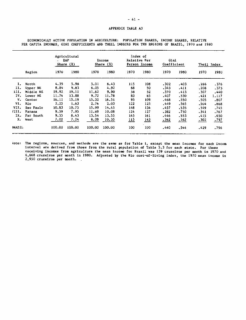
For the agricultural sector itself a marked increase in income

inequality can be discerned. All measures tell the same story. The Gini

coefficient rose from 0.44 to 0.54, the Theil index soared from 0.43 to

0.80 (Appendix Table A3), the income share of the bottom 40% fell from

15.6% to 12.4%, and the share of the top decile went from 36% to 48%

(Appendix Table A8).

- 22 -

As with the investigation of inequality among sectors,

decomposition of the Theil index is a useful tool for preliminary analysis

of the sources of this greater income disparity in the primary sector. The

Theil index for 1970, TI, may be written for agriculture as

(2) T1 = R1 +IyilTili

where R1 is a regional inequality term, the yil1s are regional income

shares, and the Til's are regional Theil indices. Using analogous

notation,

(3) T2 = R2 +EYi2Ti2i

is the same equation for 1980. In both Equations (2) and (3) i ranges from

1 to 10, corresponding to the ten regions of the 1970 census.

To allocate the change in the index we can write:

(4) T2 - T1 = (R2 - R1) + Tyil(Ti2 - Til) + (Yi2 - yil)Ti2-

The first expression on the right-hand side of Equation (4) is an effect

reflecting changed disparities among regions, the second represents changes

in inequality within regions, and the third reflects shifts in income

shares to regions with greater or lesser degrees of inequality.

Applying Equation (4) to data from Appendix Table A3, we find

that 90% of the increase in the Theil index for agriculture is due to more

- 23 -

inequality within regions. Only 4% is attributable to higher income shares

in regions with greater inequality and only 6% to greater disparity among the

ten 1970 census regions. While the fact that of the ten regions three -- the

Lower Northeast (chiefly Bahia), the Center (chiefly Minas Gerais), and

Paranda -- with 37% of agricultural income account for 56% of the increase in

inequality, may be worth exploring, clearly the phenomenon is general. For

the agricultural sector, every measure shows greater inequality for every

region. In each of the ten census regions, as may be seen from Appendix

Table A3, the Gini coefficient rose, the Theil index rose, the income share

of the bottom 40% fell, and the share of the top decile rose. In the urban

sectors, in contrast, the various regions had differing experiences.

Inequality remained roughly constant in the Northeast, declined in Sao Paulo,

and rose elsewhere.

It is useful here to briefly discuss three possible explanations

for the observed increase in inequality within agriculture. First, in

addition to lifting agricultural incomes in Brazil generally, the commodities

boom of 1979-1980 also most likely generated inequality through, for example,

the surging production of particular export crops, such as cocoa in Bahia and

soybeans elsewhere. Soybeans, cultivated on relatively large farms, probably

exercised an especially severe impact on the distribution of earnings where

this crop replaced more labor-intensive coffee, as happened in Parana. But

these location-specific explanations do not explain why inequality within

agriculture rose within every region of Brazil. More geographically diffused

sources of change must be sought.

- 24 -

A second, and perhaps most important, explanation for increased

income inequality within agriculture lies in the growth of the credit

subsidies for agriculture during the decade. With fixed nominal interest

rates, high inflation, and substantial credit allocation for agriculture the

subsidies, both expressed as rates and in volume terms, became substantial.

One study has estimated that these credit subsidies, expressed as a

proportion, amounted to 21% of the total value of agricultural output in

1980.14/ While also presenting substantial macroeconomic difficulties,

along with other, microeconomic distortionary effects, it seems incontestable

that these subsidies, and their increase, have had the effect of increasing

inequality within agriculture. First, only landowners, as contrasted to

landless workers, qualify. Second, the amount of credit, and consequent

credit subsidy bonanza, appears to be a positive function of the size of land

holdings. Despite the considerable increases in agricultural credit ceilings

through the Banco do Brasil in the late 1970s, credit rationing has still

proven necessary in the face of the demand for the subsidies. One study

(Ferreira, 1981) estimatea that only 4% of the total amount of agricultural

credit in the Northeast in 1975 went to farms of less than 10 hectares.

A third possible explanation for the observed increase of income

inequality within agriculture can be found in the theory of human capital.

In every region of Brazil average years of schooling rose for the EAP in

agriculture during the 1970's. For all Brazil the composition of the EAP

in agriculture by years of schooling was:

14/ Tyler (1981). A comparable study by Gerva'sio Resende and Milton da Mata(1981), employing a somewhat different procedure, presents an evenhigher estimate.

- 25 -

YEARS 1970 1980

0 58% 53%1 10% 7%2 12% 9%3 10% 11%4+ 11% 20%

Total 100% 100%

Human capital theory predicts that inequality rises with average

educational attainment. For Brazil in 1970, Langoni (1973, pp. 253-255)

confirms this through ginasio by finding the Gini coefficient to be 0.260

for illiterates, 0.458 for those completing primario, and 0.502 for those

completing ginasio. Human capital theory also predicts that inequality

rises with greater inequality of educational attainment.

We find the data for the rural sector of Brazil in accordance

with both of these predictions, as shown by Equation (5), in which GINI is

the Gini index of income equality for the rural sectors of each of the 23

census "states" in 1980, LAVED is the natural logarithm of the average years

of schooling of the EAP, and GED is a Gini index of inequality of years of

schooling of the EAP.

(5) GINI = -.0370 + .228 LAVED + .5887 GED

(.060) (.250)

R2 = 0.630

- 26 -

The standard errors indicate both coefficients to be significant, and the

R2 shows that these two variables explain five-eighths of the variance in

rural inequality across the states of Brazil. Appendix Table A5 displays

more regressions of this type.

These regressions do not prove causation. It may be that

inequality of years of schooling results from income inequality rather than

vice-versa, just as inequality in ownership of consumer durables results

from, but probably does not cause, income inequality. Studies which

suggest the returns to education in Brazil are quite high, particularly for

the early years, lead us to think that educational inequality in fact does

cause income inequality, especially if years of schooling is considered to

include better health and other qualities usually associated with

educational attainment. We also note that in the primary sector of Brazil

in the 1970's income inequality and educational inequality moved in

contrary directions, a further indication that educational inequality plays

an independent role.

- If the human capital interpretation of Equation (5) is accepted,

its coeffcients explain around two-fifths of the observed increase in

income inequality in the rural sector as measured by the Gini coefficient.

Appendix Table A6 shows that a 34% increase in average years of schooling

between 1970 and 1980 accompanied a decrease of GED from 0.707 to 0.660.

The first change raises inequality but the second lowers it, leaving

three-fifths of the increase to be explained. Perhaps the age structure of

the EAP changed in a relevant way over the decade. We cannot tell from the

advance tabulations. Perhaps the more detailed income questions in the

- 27 -

1980 census elicited fuller responses from the upper deciles of the primary

sector more than from others. Again, we cannot determine whether this is

so from the material at hand. At present the greater inequality within

agriculture remains partly a mystery.

The results of our analysis of the 1980 demographic census

materials can also be used to offer some interpretations regarding the

labor market. The evolution of the labor market between 1970 and 1980 is

broadly consistent with the hypothesis that, in terms of. a dualistic model,

Brazil reached a turning point during the early 1970's.15 / Over the

decade real wages roughly doubled, and this gain was shared by the lower

income groups. Income inequality may have improved slightly or may have

worsened slightly; in either case the change was small. A large rightward

shift in the demand for labor in the urban sectors pulled migrants from

rural areas, so that the share of agriculture in the labor force plunged

from 40% to 28%. This process pulled up rural wages from 37% to 50% of

urban levels. Higher urban wages also drew more women into the labor

force. For women 10 and over the participation rate rose from 19% to 27%.

Apparently women's elasticity of supply was greater at the lower skill

levels, with the result that the ratio of female to male incomes, after

rising a bit in the 1960's, lost ground in the 1970's, going from 61% to

56% for the economically active population.

The Brazilian labor market also changed in ways generally

consistent with human capital theory. Associated with higher incomes was a

15/ Morley (1982) advanced this hypothesis in a recent study.

- 28 -

rise of 40% in the average years of schooling of the labor force.

Illiteracy declined from 33% to 26% of the population 15 and over. At the

same time, in accordance with the human capital interpretation, higher

educational levels pushed income inequality up, and improved distribution of

schooling pulled it back down. The Gini coefficient for inequality of years

of schooling dropped from 0.598 to 0.499 over the decade (Appendix Table A6).

But much of the picture of the development of the labor market in

the 1970's remains unclear. One of the gaps is the distributional impact

of the higher female participation rate. In a strictly accounting sense

rising female participation had little effect on the distribution of

individual incomes. In an experiment in which we construct a hypothetical

1980 distribution of income by keeping the male and female patterns as they

were in 1980 but reducing the female participation rate to its 1970 level,

we find changes in the inequality measures for individuals only in the

third places after the decimals.

Nonetheless, the fact that a fourth of the increase in the

Brazilian labor force in the 1970's was due to the rising female labor

force participation rate probably does affect the distribution of income

noticeably through processes our methods fail to capture. First, families

have more income earners than otherwise. Is the effect concentrated on

part of the range of family incomes or spread evenly across it? Second,

women compete with men for jobs, especially at the lower end of the

spectrum of wages. Does this extra competition drive those wages down?

Investigation of these matters requires individual rather than categorical

data.

- 29 -

Another question concerns the limited integration of the national

labor market in Brazil. Wages in the Northeast average less than half of

those in the Southeast and have for decades. Why is this differential not

eliminated by inter-regional factor flows? Part of the explanation is that

labor in the Northeast is less qualified. The average number of years of

schooling in the Northeast for the EAP is only half that in the Southeast.

Moreover, some migration occurs. Had there been no inter-regional

migration at all, the population of the Northeast would have been larger

by a sixth in 1980. The effect of migration on the labor force may have

been greater still. And there may be substantial regional differences in

the cost of living, although they would be balanced by a greater

availability of public services in higher-cost areas. All in all, the

persistence of such enormous regional disparities remains a puzzle.

V. CONCLUDING REMARKS

The 1980 demographic census presents a wealth of information.

The data made available so far, in the form of advance tabulations, have

permitted us to undertake some exploratory analysis of poverty and income

inequality for 1980. The data can then be used for some comparisons

between 1970 and 1980. The results show that there has been substantial

progress in improving living standards during the 1970's. The non-income

measures of poverty attest to considerable progress, despite continued and

pressing problems of poverty. Average real incomes have also increased

substantially, even among the poorest 40% of the economically active

population. Overall income inequality did not undergo appreciable change

between 1970 and 1980. The relative stability of a high level of

- 30 -

inequality was due to two offsetting changes. On the one hand, there was

observed a large rise in rural incomes relative to urban incomes. On the

other hand, however, there was an increase in the inequality of incomes

within agriculture. The overall picture has been one of some reduction in

regional income disparities, and, in general, the available evidence

points to a reduction in absolute poverty during the 1970s. This is not to

suggest, however, that income inequality and poverty do not, or should not,

remain as principal problem areas for concern for Brazilian policy-makers.

One must also ponder whether, in view of the employment opportunities

generated during the high growth 1970s, slower economic growth, and

recession as observed in 1981-83, will not exacerbate underlying

socio-economic problems.

- 31 -

REFERENCES

Ramonaval Augusto Costa, Distribuigao da Renda Pessoal no Brasil, 1970(Rio de Janeiro: IBGE, 1977).

Frank Cowell and Fatemah Mehta, "The Estimation and Interpolation ofInequality Measures," Review of Economic Studies, April 1981,pp.273-290.

David Denslow, Jr., "Income Inequality and Poverty in Brazil: MeasuresDerived from the Advance Tabulations of the 1980 DemographicCensus," unpublished paper, 1982.

Leo da Rocha Ferreira, "Desigualdades entre Diferentes GruposSocio-Economicos na Agricultura do Nordeste," Textos para DiscussaoInterna No. 33, IPEA/INPES, Junho de 1981.

Gary S. Fields, "Who Benefits from Economic Development: AReexamination of the Brazilian Experience," American Economic Review,Vol. 67, No. 4 (September 1977), pp.570-582.

Marcos G. da Fonseca, "Um Raio-X da Distribuicao da Renda Brasileira:Uma Decomposicao do Coeficiente de Gini," Revista de EstudosEconomicos (1980).

Albert Fishlow, "Brazilian Size Distribution of Income," AmericanEconomic Review, Proceedings Vol. 62 (May 1972), pp.391-401.

M. Louise Fox, "Income Distribution Analysis in Brazil: Better Numbersand New Findings," unpublished paper, January 1982.

J.L. Gastwirth, "The Estimation of the Lorenz Curve and the GiniIndex," Review of Economics and Statistics (May 1972), pp.303-316.

Rodolfo Hoffman and J.C. Duarte, "A Distribuigao da Renda no Brasil,"Revista de Administragco de Empresas, Vol.12, No.2 (March 1972),pp.46-66.

Nanak C. Kakwani, Income Inequality and Poverty: Methods of Estimationand Policy Analysis (New York: Oxford University Press, 1980).

Peter T. Knight, "Brazilian Socioeconomic Development: Issues for theEighties," World Development, Vol. 9, No. 11/12 (December 1981), pp.1063-1082.

Peter T. Knight et al., Brazil: Human Resources Special Report, WorldBank Country Study (Washington: World Bank, October 1979.

Thomas W. Merrick, "The Impact of Access to Piped Water on InfantMortality in Urban Brazil, 1970 to 1976," World Bank, unpublishedpaper, August 1981.

- 32 -

Carlos Geraldo Langoni, Distribuicao da Renda e DesenvolvimentoEconomico do Brasil (Rio de Janeiro: Expressao e Cultura, 1973).

Constantino Lluch, "On Poverty and Inequality in Brazil," unpublishedpaper, September 1981.

Samuel Morley, Labor Market and Inequitable Growth: The Case ofAuthoritarian Capitalism in Brazil, (London: Cambridge UniversityPress, 1983).

Guy Pfefferman and Richard Webb, "The Distribution of Income inBrazil," World Bank Staff Working Paper No. 356 (September 1979).

, "Poverty and Income Distribution in Brazil,"Revista Brasileira de Economia, forthcoming in 1983.

Gervasio Castro de Resende and Milton da Mata, "Cr6dito Agricola noBrasil," IPEA/INPES, unpublished paper, 1981.

Jose W. Rossi, "0 Menor da Concentra'ao de Gini Aplicado a Dados deDistribuisao da Renda no Brasil," Revista de Estudos Economicos,forthcoming.

Henri Theil, Economics and Information Theory (Amsterdam:NorthHolland, 1967).

Vinod Thomas, "Differences in Income, Nutrition and Poverty withinBrazil," World Bank Staff Working Paper No. 505 (February 1982).

William G. Tyler, "Trade Policies and Industrial Incentives in Brazil,1980-81," INPES/IPEA, unpublished report, August 1981.

- 33 -

APPENDIX

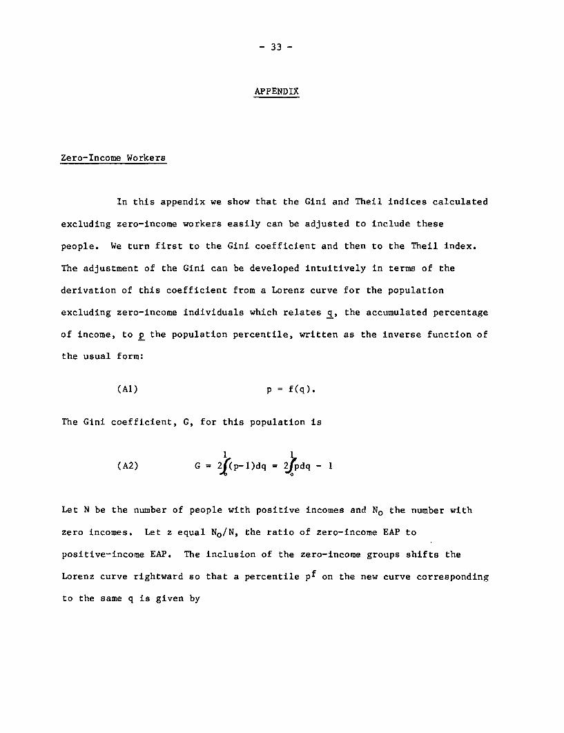
Zero-Income Workers

In this appendix we show that the Gini and Theil indices calculated

excluding zero-income workers easily can be adjusted to include these

people. We turn first to the Gini coefficient and then to the Theil index.

The adjustment of the Gini can be developed intuitively in terms of the

derivation of this coefficient from a Lorenz curve for the population

excluding zero-income individuals which relates q, the accumulated percentage

of income, to p the population percentile, written as the inverse function of

the usual form:

(Al) p = f(q).

The Gini coefficient, G, for this population is

(A2) G - 2f(p-l)dq = pjdq - I

Let N be the number of people with positive incomes and No the number with

zero incomes. Let z equal NO/N, the ratio of zero-income EAP to

positive-income EAP. The inclusion of the zero-income groups shifts the

Lorenz curve rightward so that a percentile pf on the new curve corresponding

to the same q is given by

- 34 -

(A3) f p+z

Hence the Gini coefficient, Gf, for the full group is

(A4) Gf = 4jpfdq - I

After substitution from (A3) and some manipulation this may be written

Gf= 1 (2 dg - 1) + -+-1+Iz jf 1+z

0

(A5) Gf = G + - (1 - G).

1+z

Thus Gini coefficient for the full population is simply the Gini for the

positive-income group plus the ratio of the zero-income individuals to the

full population multiplied by the complement of the original Gini.

The derivation of the adjustment to the Theil index is direct.

The Theil index, T, for positive-income recipients may be written

(A6) T =IyilnyiN

- 35 -

where yi is the income share of the ith person and "+" indicates summation

over positive-income individuals. Defining z as before, the Theil index,

Tf, for the full population is

(A7) T= E yilnyiN(l+z) + E yilnyiN(1+z)0 +

where "o" indicates summation over those with zero incomes and each person

is now one out of N(1+z) instead of N individuals. The first term on the

right-hand side of (A7) goes to zero as the yi go to zero. Noting this and

that (A8) Yi = 1

we can write (A7), substituting from (A6), as

(A9) Tf = T + ln(1+z)

Hence inclusion of a zero-income group augments both the Gini coefficient

and the Theil 'index in simple ways.

In summary, we have excluded zero-income members of the EAP from

our calculations to aid comparison with Langoni's figures for 1970 and

because their inclusion weakens the association between individual and

family income deciles. Including zero-income recipients' raises the

agricultural inequality measures markedly but does not change the general

picture: during the 1970s, overall inequality remained roughly constant

while rising sharply within agriculture.

- 36 -

The 1970 Upper Coding Limit

As noted in the text, the determination of changes in the degree

of inequality between 1970 and 1980 in Brazil is complicated by the

existence in 1970 of an upper coding limit on income. All incomes of 9998

or more cruzeiros per month were coded as 9998, a figure which after

adjustment for inflation by the Rio cost-of-living index corresponds to

285,000 cruzeiros of 1980, or approximately US$5,215. It is about 30

times the mean income for 1970. This truncation of the upper tail of the

income distribution reduces both the Gini coefficient and the Theil index.

The effect of this truncation on the Gini coefficient may be

viewed through its impact on the Lorenz curve. Let V.Y1 be the1=1

,.~ *

amount of true income and ŽYi be the amount of coded income, with

G calculated from the distribution f(Y) and G* calculated from the

distribution f*(Y*), where f*(Y*) is identical to f(Y) up to the upper

coding limit. The respective Lorenz curves are L(q,p) and L*(q*,p), where

p is the percentile of recipients while q and q* are the accumulated

percentages of income. We define w to be the ratio of coded to actual

total income:

N * N(A10) w= Yi/ : i

If wdia psh oli pctei=l i=l

If we designate p as the population percentile at the upper

- 37 -

coding limit, then using an argument similar to that developed in the

previous section -- with integration over p instead of q, and using limits

-- it may be shown that

(All) m 1 G = G* + (1-w)(1-G*).

Equation (All) serves as a good approximation for our purposes since the

area between the Lorenz curve and the 45-degree line to the right 2f p is

quite small.

A crude estimate of w, the ratio of coded to actual income, may

be obtained from data presented by Lluch (1981). In a random selection of

16,310 families with reported incomes from the 1970 Public Use Sample, he

found 19 coded at the upper limit, or 0.12%. Partly for simplicity let us

suppose that for individuals the ratio would be slightly lower, say one per

thousand. The average income for individuals was 282 cruzeiros per mnnth.

As an approximation, take the upper coding limit to be 10,000 instead of

9,998. A person coded at the upper limit would have, out of a thousand

typical individuals, a reported income equal to 3.55% of the total reported

income of 282,000. Suppose this person's actual income were 20,000

(corresponding to a Pareto distribution with alpha equal to two). Then w

would equal 282,000/292,000 or .966, and Langoni's 1970 Gini of .565 would

be raised to .580, within the range of error of our estimate for 1980 of

.590.

- 38 -

It is convenient to use this same numerical illustration to

discuss the effect of the upper coding limit on the Theil index. The Theil

index derived from coded incomes, T*, can be decomposed as

(A12) T* = (272/282)ln[(272/282)/.999] + (10/282)ln[(10/282)/.001]

+ ( 2 7 2 / 2 8 2 )TL + (10/ 2 8 2 )TH

* *where TL and TH are the within-group Theil indices for those below the

coding limit and those at or above it, respectively, based on coded

incomes. Since all incomes in the upper group are coded at the same value,

10,000, TH is zero. Hence, using Langoni's value of .6629 for T , TLis found to be .5912.

Now consider T, the Theil index based on actual incomes. If the

average income of those in the upper group is 20,000, we have

(A13) T = (272/292)ln[(272/292)/.999] + (20/292)ln[(20/292)/.001]

+ (272/292)(.5912) + (20/292)TH,

where TH is the within-group Theil index for those at or above the coding

limit. The within-group index is unaffected by removal of the coding

limit. If the upper distribution is Pareto with alpha equal to two, then,

using a formula derived by Theil (1967, p. 98), TH equals .3068 and T

equals .796, which is higher than our estimate for 1980 of .704.

APPENDIX TABLE Al

PERCENTAGE OF BRAZILIAN HOUSEHOLDS (PERMANENT)POSSESSING SELECTED DURABLE CONSUMERS GOODS AND SERVICES

BY REGION AND LOCATION, 1970 AND 1980

1970 1980

RegionUrban Rural Total Urban Rural Total

BRAZIL a/

(Coal) 5.0 1.9 3.9 4.1 8.7 5.6Stove (Gas) 69.3 5.5 42.7 83.3 12.7 61.3

(Wood) 20.9 78.9 45.1 11.4 77.5 32.0

Telephone n.a. n.a. n.a. 17.5 .9 12.4Electricity 75.6 8.4 47.6 88.5 20.6 67.4Radio 72.4 40.1 58.9 79.3 68.0 75.8

Refrigerator 42.5 3.2 26.1 66.2 12.6 49.5Television 40.2 1.6 24.1 73.1 14.7 54.9

Automobile 13.7 2.5 9.0 28.3 9.5 22.4

NORTHEAST b/

(Coal) n.a. n.a. n.a. 19.1 16.3 17.7

Stove (Gas) n.a. n.a. 18.7 63.6 8.0 35.7(Wood) n.a. n.a. 49.0 15.6 74.4 45.2

Telephone n.a. n.a. n.a. 9.2 .5 4.8Electricity n.a. n.a. 23.3 76.1 8.3 42.0Radio n.a. n.a. 34.6 64.6 59.1 61.8Refrigerator n.a. n.a. 9.2 44.0 3.9 23.8Television n.a. n.a. 6.3 50.4 4.6 27.4Automobile n.a. n.a. 3.0 15.8 2.8 9.3

SOUTHEAST c/

(Coal) n.a. n.a. n.a. - -


Telephone n.a. n.a. n.a. 20.2 1.3 16.2Electricity n.a. n.a. 61.6 93.4 36.5 81.3

Radio n.a. n.a. 71.9 84.6 80.6 83.7Refrigerator n.a. n.a. 35.6 74.0 23.0 63.2Television n.a. n.a. 34.4 81.1 27.5 69.7

Automobile n.a. n.a. 12.4 32.5 17.2 29.3

FRONTIER d/

(Coal) n.a. n.a. n.a. 4.0 11.2 6.9


Telephone n.a. n.a. n.a. 14.9 .9 9.3

Electricity n.a. n.a. 28.1 77.8 10.8 51.0

Radio n.a. n.a. 47.5 69.3 57.4 64.5Refrigerator n.a. n.a. 14.0 53.1 8.1 35.1

Television n.a. n.a. 10.1 59.5 7.3 38.6Automobile n.a. n.a. 5.1 22.2 6.6 16.0

Notes: a/ In 1970, 55.9% of the population in Brazil lived in urban areas. In 1980, thefigure was 67.6%.

b/ In 1970, 41.8% of the population in the Northeast lived in urban areas. In1980, the figure was 50.4%.

c/ In 1970, 64.4% of the population in the Southeast lived in urban areas. In1980, the figure was 77.3%.

d/ In 1970, 46.8% of the population in the Frontier lived in urban areas. In1980, the figure was 60.7%.

* sign -" means percentage of less than 0.1.

SOURCES: IBGE, Censo Demografico, Brasil-1970, Volume 1 and Tabulacoes Avancadn s do CensoDemografico, Brasil-1980, Volume 1 - Tomo 2 (Rio de Janeiro: IBGE, 1973 and1981)..

- 40 -

APPENDIX TABLE A2

ECONOMICALLY ACTIVE POPULATION IN URBAN OCCUPATIONS: POPULATION SHARES, INCOME SHARES, RELATIVEPER CAPITA INCOMES, GINI COEFFICIENTS AND THEIL INDICES FOR TEN REGIONS OF BRAZIL, 1970 and 1980

Index ofUrban EAP Income Relative Per GiniShare (X) Share (X) Person Income Coefficient Theil Index

Region 1970 1980 1970 1980 1970 1980 1970 1980 1970 1980

I. North 2.60 3.38 2.24 3.06 87 91 .527 .558 .575 .647II. Upper NE 2.10 2.17 1.06 1.18 51 54 .532 .569 .579 .682

III. Middle NE 11.03 10.57 6.99 6.90 64 65 .601 .596 .762 .770IV. Lower NE 5.90 5.78 4.37 4.64 75 80 .572 .578 .701 .668V. Center 11.77 11.77 8.45 9.75 72 83 .542 .556 .609 .645

Vl. Rio 16.14 13.76 20.21 17.41 126 127 .516 .577 .530 .669VII. Sao Paulo 30.76 30.31 39.21 35.15 129 116 .531 .522 .586 .534

VIII. Parana 5.24 5.56 4.67 5.30 90 95 .514 .566 .531 .695IX. Far South 10.09 10.77 9.12 10.82 91 100 .506 .547 .528 .635X. West 4.39 5.94 3.69 5.80 85 97 .529 .595 .583 .731

BRAZIL 100.00 100.00 100.00 100.00 100 100 .552 .565 .622 .648

Note: EAP stands for economically active population. Calculations in this table are limited to members ofthe EAP who received a positive income and stat ed the amount to the census-taker. NE stand forNorhteast. The regions are: I. Roraima, Acre, Amapa, Rond6nia, Para, and Amazonas; II. Maranhaoand Piaui; III. Ceara, Rio Grande do Norte, Paraiba, Pernambuco, and Alagoas; IV. Sergipe and Bahia;V. Minas Gerais and Espirito Santo; VI. Rio de Janeiro; VII. Sao Paulo; VIII. Parana; IX. SantaCatarina and Rio Grande do Sul; X. Mato Grosso do Sul, Mato Grosso, Goias, and the Distrito iederal.The 1970 data are from Langoni (1973, pp. 300-309). Langoni's inequality measures are calculated fromILIuIvIouaJ aaEa. ine itou figures are calculated from the Tabulacoes Avangadas of the 1980 demographiccensus of Brazil. For estimating inequality measures we used the number of people in each incomeinterval from Table 5.2 and estimated the mean income for each income interval be weighting the intervalmeans for urban males and females in Table 5.3 by male and female interval numbers in Table 5.2 state bystate. Bounds on the Gini coefficients were calculated using Method I by Gastwirth (1972) and those on theTheil index with the technique described by Theil (1967). Point estimates of the Gini and Theilmeasures were derived from these bounds using the "one-third, two-thirds" rule adovcated by Cowell and

Mehta (1982). The upper bound on coding the income data used by Langoni was approximately 35 times themean income, affecting perhaps 1% of the population. We do not know if there was an upper bound on the1980 data. If so it was at 70 or more times the mean income.

For both 1970 and 1980 "urban" occupations are all but agriculture. For this group the mean income forBrazil was 378 cruzeiros per month in 1970 and 13,914 cruzeiros per month in 1980. Adjusted by the Riocost-of-living index to August 1980 cruzeiros, the 1970 mean income in 8,023. The Gini coefficient forthe EAP for urban populations for all Brazil in 1970 is calculated through the application of theGastwirth method to data aggregated with a quadratic approximation technique. For comparison, the Theilindex derived with these methods is .629, close to the value of .622 obtained with the decompositionformula for the Theil index.

- 41 -

APPENDIX TABLE A3

ECONOMICALLY ACTIVE POPULATION IN AGRICULTURE: POPULATION SHARES, INCOME SHARES, RELATIVEPER CAPITA INCOMES, GINI COEFFICIENTS AND THEIL INDICES FOR TEN REGIONS OF BRAZIL, 1970 and 1980

Agricultural Index ofI EAP Income Relative Per GiniShare (X) Share (X) Person Income Coefficient Theil Index

Region 1970 1980 1970 1980 1970 1980 1970 1980 1970 1980

I. North 4.35 5.98 5.01 6.43 115 108 .302 .403 .166 .376II. Upper NE 8.84 9.83 6.05 4.92 68 50 .343 .411 .208 .375III. Middle NE 19.92 19.11 11.62 9.90 58 52 .370 .413 .307 .440IV. Lower NE 11.74 13.88 9.72 11.78 83 85 .407 .530 .421 1.117V. Center 16.11 15.19 15.32 16.51 95 109 .468 .550 .505 .807

VI. Rio 2.25 1.63 2.76 2.03 122 125 .449 .565 .504 .868VII. Sao Paulo 10.83 10.75 15.99 14.45 148 134 .457 .535 .549 .745IIII. Parana 9.59 7.95 11.89 10.08 124 127 .382 .750 .341 .767IX.. Far South 9.35 8.43 13.54 13.55 145 161 .446 .553 .415 .650X. West 7.02 7.24 8.09 10.35 115 143 .362 .562 .302 .797

3RAZIL 100.00 100.00 100.00 100.00 100 100 .440 .544 .429 .796

iote: The regions, sources, and methods are the same as for Table 1, except the mean incomes for each incominterval are derived from those from the rural population of Table 5.3 for each state. For thosereceiving incomes from agriculture the mean income for Brazil was 139 cruzeiros per month in 1970 and6,668 cruzeiros per month in 1980. Adjusted by the Rio cost-of-living index, the 1970 mean income is2,950 cruzeiros per month.

- 42 -

APPENDIX TABLE A4

ECONOMICALLY ACTIVE POPULATION IN 1980 BY STATES OF BRAZIL.AVERAGE INCOMES, GINI COEFFICIENTS AND THEIL INDICES FUR AGRICULTURAL AND FOR URBAN OCCUPATIONS

Population /a Mean Income /b Gini Theil

State Urban Agricul. Urban Agricul. Urban Agricul. Urban Agricul.

1. Rondonia /c 172 131 12,085 7,131 .521 .424 .547 .3792. Amazonas 256 154 14,964 7,267 .561 .419 .641 .5303. Para 567 365 11,674 7,145 .562 .389 .672 .3174. Maranhao 380 776 7,398 3,441 .538 .403 .591 .3365. Piaui 259 292 7,814 3.077 .609 .426 .812 .489

6. Ceara 929 601 8,335 3,563 .612 .444 .780 .5197. Rio Grande do Norte 342 191 7,891 3,445 .561 .402 .674 .4098. Paraiba 412 314 7,524 3,110 .563 .407 .680 .3969. Pernambuco 1,157 678 10,768 3,456 .603 .388 .810 .380

10. Alagoas 276 294 8,331 3,586 .558 .411 .685 .467

11. Sergipe 189 128 10,099 4,193 .583 .425 .717 .47812. Bahia 1,514 1,381 11,298 5,793 .577 .537 .662 1.16213. Minas Gerais 3,017 1,462 11,454 7,158 .554 .550 .633 .81014. Espirtio Santo 453 191 12,004 7,896 .568 .551 .722 .78415. Rio de Janeiro 4,056 177 17,603 8,324 .577 .565 .669 .868

16. Sao Paulo 8,935 1,170 16,137 8,953 .522 .535 .534 .74617. Parana 1,638 865 13,284 8,453 .566 .750 .695 .76618. Santa Catarina 891 292 12,238 9,735 .513 .466 .569 .430IV. Rio urande do Sul 2,284 624 14,662 11,171 .3bo .58b .b5l .13t.U. r4tc Uro^bo Qo b6l J19 6ib 12,6U4 11,511 .591 .618 .74b 1.u16

21. Mato Grosso 219 141 13,329 8,036 .595 .460 .804 .49522. Goias 744 477 10,668 9,121 .571 .558 .670 .76623. Distrito Federal 442 9 19,421 17,922 .593 .660 .675 .856

BRAZIL 29,481 10,874 13,914 6,668 .564 .544 .648 .796

Note: The sources and methods are the same as those for 1980 in Tables I and 2. The heading "Agricul." refers tcagricultural occupations and "Urban" to all other.

/a Population is in thousands and refers to members of the economically active population who arereceiving a positive income and stated the amount to the census-taker.

/b Mean income is in cruzeiros per month. At the time of the census, the exchange rate was equal toCr$54.65 per US dollar.

/c Rondonia, Acre, Roraima, and Amapa.

APPENDIX TABLE A5

REGRESSIONS OF INCOME INEQUALITY MEASURES ON THE LOGARITHM OF AVERAGESCHOOLING AND A GINI INDEX OF SCHOOLING INEQUALITY, 1980

Dependent CoefficientsRegression Year Observations Occupations Variable Constant LAVED GED R2

1. 1980 23 States All GINI -. 0648 .2364(.0598) .6029(.1592) 0.4392. 1980 23 States Rural GINI -. 0375 .2270(.0595) .5872(.2498) 0.6293. 1980 23 States Urban GINI -. 0750 .2377(.0875) .6038(.1842) 0.3684. 1980 46 States Pooled GINI -. 2303 .1307(.0269) .3191(.1335) 0.6415. 1980 23 States All TOP40 .3840 .1622(.0338) .3721(.0900) 0.5766. 1980 23 States All LOW40 .3199 -. 0868(.0169) -. 1906(.0405) 0.635

Notes: The dependent variable GINI is the Gini Index of income inequality for each group. The dependent variable TOP40is the income share of the highest 40% of individual earners and LOW40 is the lowest 40%. The regressors are LAVED,the natural logarithm of average years of schooling, and GED, a Gini index of inequality of years of schooling. Thesemeasures are calculated from Tabulacoes Avancadas do Censo Demografico, 1980, Table 5.2.

Under the heading "Occupations" the word "pooled" refers- to-placing both urban and rural occupations in oneregression as separate observations. Thus, in Regression 4, this amounts to having 23 rural plus 23 urban "regions.

Standard errors are in parentheses. All variables are significantly different from zero at the 5% level.

- 44 -

APPENDIX TABLE A6

AVERAGE YEARS OF SCHOOLING AND INEQUALITY OF YEARS OF SCHOOLING,THREE REGIONS OF BRAZIL, 1970 AND 1980

Total Economically Active Population

Average Years Gini Index of SchoolingRegion 1970 1980 1970 1980

Southeast 3.71 4.95 .506 .416Northeast 1.52 2.50 .787 .691Frontier 2.44 3.82 .635 .524

Brazil 2.98 4.19 .598 .499

Rural Occupations


Southeast 1.74 2.45 *.585 .492Northeast 0.44 0.60 .854 .836Frontier 1.07 1.59 .680 .641

Brazil 1.16 1.56 .707 .660

Urban Occupations


Southeast 4.76 5.61 .428 .374Northeast 3.26 4.31 .612 .514Frontier 4.13 5.10 .496 .420

Brazil 4.43 5.31 .469 .406

Note: These measures are calculated from Tabulacoes Avancadas do CensoDemografico, 1970, Table 6, and Tabula,oes Avangadas do CensoDemografico, 1980, Table 5.2. They are approximations derived frominterval data. The regions are defined in Table 7.

- 45 -

APPENDIX TABLE A7

INCOME DECILES FOR THREE REGIONS OF BRAZIL, ECONOMICALLYACTIVE POPULATIONS, 1970 AND 1980

SOUTHEASTAccumulated

Percentage of Income Percentage of Income Average Income PercentageDecile 1970 1980 1970 1980 1970 1980 Change

1 1.32 1.27 1.32 1.27 1,284 1,767 382 3.61 3.70 2.29 2.43 2,226 3,382 523 6.63 6.77 3.02 3.07 2,938 4,280 464 10.88 10.50 4.25 3.72 4,137 5,186 255 16.23 15.11 5.35 4.61 5,220 6,423 236 22.11 20.85 5.88 5.75 5,734 8,002 407 29.70 28.32 7.59 7.46 7,388 10,394 418 40.27 38.53 10.57 10.21 10,298 14,219 389 55.36 53.90 15.09 15.37 14,719 21,396 4510 100.00 100.00 44.64 46.10 43,503 64,200 48

AVERAGE 9,756 13,925 43

NORTHEASTAccumulated


1 1.14 1.42 1.14 1.42 513 1,000 952 3.61 3.72 2.48 2.31 1,113 1,630 463 7.11 6.58 3.49 2.85 1,568 2,015 284 11.48 10.25 4.37 3.67 1,969 2,595 325 16.65 14.82 5.17 4.57 2,310 3,227 406 22.56 20.21 5.91 5.39 2,653 3,806 437 29.89 26.79 7.33 6.58 3,281 4,644 428 39.14 35.86 9.25 9.07 4,137 6,408 559 52.15 49.53 13.01 13.67 5,848 9,654 65

10 100.00 100.00 47.85 50.47 21,452 35,637 66AVERAGE 4,478 7,062 58

FRONTIERAccumulated


1 2.19 1.15 2.19 1.15 1,484 1,244 -162 5.52 3.57 3.33 2.42 2,254 2,617 163 9.48 6.95 3.96 3.38 2,681 3,651 364 14.51 10.69 5.03 3.75 3,423 4,048 185 20.60 14.59 6.09 3.89 4,137 4,206 26 27.09 19.47 6.49 4.88 4,394 5,272 207 35.22 26.22 8.12 6.75 5,505 7,300 338 44.57 35.71 9.36 9.49 6,333 10,256 629 59.04 50.38 14.47 14.67 9,813 15,854 62

10 100.00 100.00 40.96 49.62 27,756 53,634 93AVERAGE 6,790 10,808 59

Note: The figures for 1970 are based on Table 8 of the Tabulacoes Avancadas do CensoDemografico, 1970. The methods for 1970 are described in Denslow (1982). Ths figures for1980 are from Tables 5.2 and 5.3 of the Tabulacoes Avangadas do Censo Demografico, 1980.The methods are those of previous tables. For both years the data describe members of theeconomically active population with positive incomes and reporting those incomes to censustakers.

- 46 -

APPENDIX TABLE A8

INCOME DECILES FOR RURAL OCCUPATIONS, THREEREGIONS OF BRAZIL, 1970 AND 1980

ALL BRAZILAccumulated


1 2.16 1.86 2.16 1.86 853 1,241 452 5.69 4.61 3.53 2.74 1,392 1,826 313 10.03 8.02 4.34 3.41 1,712 2,269 334 15.56 12.40 5.53 4.39 2,180 2,921 345 22.21 17.65 6.65 5.24 2,623 3,491 336 29.59 23.61 7.38 5.96 2,910 3,965 367 38.76 30.51 9.17 6.91 3,614 4,598 278 49.82 39.48 11.06 8.97 4,360 5,968 379 63.71 52.11 13.89 12.63 5,477 8,409 54

10 100.00 100.00 36.29 47.89 14,308 31,874 123AVERAGE 3,943 6,656 69



1 2.14 1.76 2.14 1.76 1,027 1,511 472 5.77 4.36 3.63 2.60 1,740 2,235 283 10.30 7.90 4.53 3.54 2,168 3,042 404 15.53 12.18 5.23 4.28 2,511 3,673 465 21.43 16.94 5.90 4.76 2,824 4,092 456 29.16 22.29 7.72 5.35 3,708 4,595 247 38.05 28.91 8.89 6.61 4,251 5,680 338 48.54 37.52 10.49 8.61 5,021 7,400 479 61.36 50.75 12.82 13.23 6,133 11,364 85

10 100.00 100.00 38.63 49.25 18,457 42,302 129AVERAGE 4,793 8,589 79



1 1.86 2.30 1.86 2.30 513 951 852 5.68 5.92 3.83 3.62 1,027 1,501 463 10.93 10.30 5.25 4.38 1,426 1,815 274 17.38 15.32 6.45 5.02 1,740 2,080 205 24.91 21.41 7.53 6.08 2,054 2,519 236 33.43 28.66 8.52 7.25 2,310 3,004 307 42.87 37.08 9.44 8.42 2,567 3,488 368 53.42 46.68 10.55 9.60 2,852 3,977 399 68.13 59.24 14.71 12.56 3,993 5,200 30

10 100.00 100.00 31.87 40.76 8,671 16,880 95AVERAGE 2,710 4,142 53

FRONTIERAccumulated


1 3.47 2.12 3.47 2.12 1,568 1,791 142 8.35 5.31 4.88 3.19 2,226 2,697 213 13.95 9.40 5.60 4.09 2,539 3,463 364 20.11 14.11 6.16 4.71 2,796 3,984 435 27.78 19.48 7.67 5.38 3,480 4,547 316 36.82 25.91 9.04 6.43 4,107 5,439 327 46.32 33.67 9.50 7.76 4,308 6,564 528 57.81 43.09 11.49 9.41 5,220 7,962 539 70.98 56.23 13.17 13.14 5,990 11,116 86

10 100.00 100.00 29.02 43.77 13,179 37,028 181AVERAGE 4,536 8,459 86

Note: The figures for 1970 are based on Table 8 of the Tabulacoes Avangadas do CensoDemografico, 1970. The methods for 1970 are described in Denslow (1982). The figures for1980 are from Tables 5.2 and 5.3 of the Tabulacoes Avancadas do Censo Demografico, 1980.The methods are those of previous tables. For both years the data describe members of theeconomically active population with positive incomes and reporting those incomes to censustakers.

- 47 -APPENDIX TABLE A9

INCOME DECILES FOR URBAN OCCUPATIONS, THREEREGIONS OF BRAZIL, 1970 AND 1980

ALL BRAZILAccumulated


1 1.04 1.05 1.04 1.05 1,133 1,389 222 3.19 3.01 2.14 1.96 2,333 2,582 113 6.53 5.88 3.34 2.87 3,636 3,787 44 10.80 9.37 4.27. 3.49 4,645 4,610 -15 15.81 13.81 5.01 4.44 5,453 5,864 76 21.53 19.45 5.72 5.64 6,194 7,444 207 29.39 26.85 7.86 7.40 8,561 9,763 148 39.97 37.10 10.59 10.25 11,522 13,530 179 55.14 52.85 15.16 15.75 16,498 20,796 26

10 100.00 100.00 44.86 47.15 48,815 62,231 27AVERAGE 10,88 1 13,199



1 1.23 1.30 1.23 1.30 1,484 1,965 322 3.63 3.84 2.40 2.54 2,882 3,845 333 7.32 6.99 3.68 3.14 4,422 4,754 84 11.68 10.86 4.36 3.88 5,220 5,862 125 16.43 15.64 4.75 4.78 5,677 7,222 276 22.41 21.59 5.98 5.96 7,159 9,007 267 30.58 29.21 8.17 7.62 9,784 11,524 188 41.00 39.65 10.42 10.43 12,495 15,779 269 56.18 55.12 15.18 15.47 18,171 23,400 29

10 100.00 100.00 43.82 44.88 52,489 67,874 29AVERAGE 11,967 15,123 2



1 0.73 1.11 0.73 1.11 513 1,060 1062 2.57 3.01 1.84 1.90 1,312 1,818 393 5.36 5.70 2.80 2.68 1,997 2,564 284 9.06 9.27 3.70 3.57 2,653 3,412 295 13.96 13.56 4.91 4.29 3,537 4,096 166 19.73 19.05 5.76 5.49 4,137 5,245 277 27.12 26.22 7.39 7.17 5,306 *6,853 298 36.68 35.89 9.56 9.67 6,875 9,236 349 51.56 51.27 14.88 15.38 10,697 14,694 37

10 100.00 100.00 48.43 48.73 34,773 46,552 34AVERAGE 7,189 9,553 33

FRONTIERAccumulated


1 1.44 0.82 1.44 0.82 1,341 1,014 -242 4.06 2.89 2.62 2.07 2,425 2,557 53 7.72 5.96 3.66 3.06 3,395 3,782 114 12.21 9.70 4.49 3.74 4,165 4,613 115 17.34 14.29 5.13 4.60 4,764 5,672 196 23.57 19.90 6.23 5.60 5,762 6,917 207 31.27 26.81 7.70 6.91 7,131 8,528 208 41.69 36.26 10.42 9.46 9,670 11,671 219 56.26 51.22 14.57 14.96 13,522 18,464 37

10 100.00 100.00 43.74 48.78 40,565 60 196 48AVERAGE 9,271 12,3 r

Note: The figures for 1970 are based on Table 8 of the Tabulazoes Ayanjadas do CensoDemografico, 1970. The methods for 1970 are described in Denslow figures for1980 are from Tables 5.2 and 5.3 of the Tabulacoes Avangadas do Censo Demografico, 1980.The methods are those of previous tables. For both years the data describe members of theeconomically active population with positive incomes and reporting those incomes to censustakers.

World BankPublicationsof RelatedInterest

NEW

rhe Determinants of Labour income countries in terms of a num- Economic Growth andEarnings in Developing ber of socioeconomic indicators, it is Employment in Chinanetropolises: Estimates noted that there are large regional Thomas G. Rawskidisparities between the northeast andfirom Bogota and Call, the southeast with the northeast far- Examines how China's agriculturalColombia ing about the same as most low- sector has made significant stridesRakesh Mohan income countries. toward full employment for a labor

force of nearly half a billion persons.Examines the patterns of behavior World Bank Staff Working Paper No.Implicit in the variation of labor earn- 505. February 1982. 91 pages (Includ- Oxford Uniuersity Press, 1979.ings in Bogota and Cali, Colombia. ing references, map). 208 pages (including maps, bibliogra-

World Bank Staff Working Paper No. Stock Nlo. WP-0505. $3.00. phy, index).498. October 1981. 135 pages (includ- LC 79-19550. ISBN 0-19-520151-5,ing 2 appendixes, bibliography). $18.95 hardcover. ISBN 0-19-520152-3,Stock No. WP-0498. $5.00. The Distribution of $7.95 paperback.

Income In Brazil French: Croissance et emploi en Chine.Guy P. Pfeffermann and Economica, 1980.

NEW Richard C. Webb ISBN 2-7178-0282-7, 39 francs.World Bank Staff Working Paper No.

Differences in Income, 356. September 1979. 116 pages Spanesh: Crecimiento economico ylMutrition, and Poverty (Including 2 appendixes). empleo en China. Editorial Tecnos,

iinod Thoras Stock No. WP-0356. $5.00. ISBN 84-309-0871-4, 600 pesetas.

Regional disparities in living stan-iards in Brazil are examined and Employment Patterns!stimates for real income and nutri- and Income Growth:onal levels and poverty for majorirban and rural areas are provided. Joseph J. Stern andUlthough the growth rate of the coun- Jeffrey D. Lewisry surpasses the average for mostJeveloping countries and the country World Bank Staff Working Paper No.,erforms as well as many middle- 419. September 1980. 70 pages

(including bibliography, 2 appen-dixes).Stock No. WP-0419. $3.00.

,mployment Policy in Household Income or Income Distribution PolicyWeveloping Countries: Household Income in the Developing Coun-L Survey of Issues per Capita in Welfare tries: A Case Study of Koreamnd Evidence Comparisons Irma Adelman andyn Squire Gautam Datta and Sherman Robinsonow rates of growth in industrial Jacob Meerman Seeks to answer the question of howmployment, high rates of unemploy- World Bank Staff Working Paper No. much can actually be done toient among new entrants to the 378. Bank Staff Work ing improve income distribution byrban labor market, and low levels of 378. March 1980. 32 pages (including means of a dynamic generalibor productivity and remuneration 3 appendixes, references). equilibrium model for investigatingre the three issues addressed in this Stock No. WP-03 78. $3.00. the potential impact of standardtudy. The author identifies the impor- policy instruments and programsint determinants of labor demand intended to improve the relative andnd supply and the extent to which How Segmented is the absolute incomes of the poor.ie growth of labor demand has been Bogota Labor Market? Stanford University Press, Stanford,

dvanced-by inappropriate policies. Gary S. Fields California 94305, U.S.A. (except thein the demand side, industrial trade World Bank Staff Working Paper No. United Kingdom and the Common-olicy, agricultural growth, and the 434. October 1980. 99 pages (includ- wealth Market). 1978 . Oxford Universityperation of capital markets are ing bibliography). Press (except Mexico, United States,iscussed; on the supply side, atten- Stock No WP-0434 $ and Canada). 1978. 364 pages (includ-on is focused on population and ' ' ing 6 appendixes, index).ducation policy. LC 76-14269. ISBN 0-8047-0925-4

xford University Press, 1981. 242 Incidence of Poverty and (Stanford), $12.50 hardcover.ages (including bibliography, index). the Characteristics of ISBN 0-19-920084-X (Oxford), £7.50

C 81-2844. ISBN 0-19-520266-X, the Poor in Peninsular hardcover.16.95 (£11.50) hardcover, ISBN Malaysia, 1973-19-520267-8, $7.95 (£5.00) Pravin Visaria Income Inequality andaperback. Examines the results of the Poverty: Methods of Estima-

Household Expenditure and Income tion and Policy Applications

irowth and Equity in Semi- Survey conducted in peninsulari ~~~~~~~~Malaysia during 1973 in order to Nanak C. K~akwanindustrialized Countries understand better the correlates Deals with income distributionoel Bergsman of poverty. methods and their economic

'orld Bank Staff Working Paper No. World Bank Staff Working Paper No. applications.51. August 1979. ii + 113 pages 460. May 1981. viii + 213 pages Oxford University Press, 1980. 432ncluding references). (including statistical appendix). pages (including bibliography,

tock No. WP-0351. $5.00. Stock No. WP-0460. $10.00. indexes).LC 80-14229. ISBN 0-19-520227-9,

irowth with Equity: Income Distribution $12.95 paperback.'he Taiwan Case and Poverty in Mexicoohn C. H. Fei, Gustav Ranis, Joel Bergsman NEWnd Shirley W. Y. Kuo World Bank Staff Working Paper No.

itroduces a method for tracing 395. July 1980. 46 pages (including Inequality and Povertyie inequality of family income to references). in Malaysia:ie inequality of various kinds of Stock No. WP-0395. $3.00. Measurement andmctor income and the sharesf factor income in family income. Sudhir Anand

ixford University Press, 1980. An account of income inequalities44 pages (including index). and poverty in Malaysia. The research

C 79-23354. ISBN 0-19-520115-9, is policy oriented and the findings, to27.50 (£10.25) hardcover; which the author's statistical tech-;BN 0-19-520116-7, $12.95 nique is applied, are thoroughlyC4.25) paperback. discussed. A range of issues is

covered, from data problems to con- regarding links between human Studies the evolution of the structureceptual questions arising with respect development and labor productivity of consumer preferences as a func-to measurement. and focuses on policy measures tion of economic development.

Oxford Uniuersity Press. 1982. 384 aimed at raising theodutvt o f Oxford University Preso, 1977. 312the poor and promoting economic OxodUiestPrs.17.32pages (including bibliography, index). development. pages (including bibliography,

LC 81-14178. ISBN 0-19-520153-1, World Bank Staff Working Paper No. indexes).$27.50 hardcover. 497. October 1981. in + 70 pages LC 77-3442. ISBN 0-19-920097-1,

(includintobe iog +70hage $22.50 hardcover;(including bibliography). ISBN 0-19-920100-5, $12.95

International Migrant Stock No. WP-0497. $3.00. paperback.Workers' Remittances:Issues and Prospects NEWGurushri Swamy TePolicy interventions for

A background study for World ~Technological Innovation inA background study for World Manpower and International Developing CountriesDevJelopment Report 1981. Putstogether available data on interna- Labor Migration in the Mid- Charles Coopertional migrant workers' remittances to dle East and North Africa World Bank Staff Working Paper No.developing countries and analyzes Ismail Serageldin, James A. 441. December 1980. 59 pagesthe regional structure of and growth Socknat, Stace Birks, Bob Li, (including references).in these flows. Relates the flow of anClvA.Scairemittances to the level of and fluc- an ive . inclair Stock No. WP-0441. $3.00.tuations in economic activity and to This study of labor market trends ininflation in the host countries and the region from 1975 to 1985attempts to forecast future demand analyzes the demand for and supply Poverty and Growthfor migrant labor and the likely of manpower by country, sector, in Kenyagrowth in remittances. occupation, sex, educational level, Paul Collier and Deepak Lal

and ethnic composition. It indicatesWorld Bank Staff Working Paper No. the sources and destinations of World Bank Staff Working Paper No.481. August 1981. 64 pages (including workers and examines the social and 389. May 1980. 76 pages (including2 appendixes, bibliography). economic effects of migration for 2 appendixes, bibliography).

Stock No. WP-0481. $3.00. both importers and exporters, par- Stock No. WP-0389. $5.00.ticularly the implications forStcNoWP08.300government policy and planning.

Labor Migration Oxford University Press.1983. About Poverty and Unemploymentfrom Bangladesh to 224 pages. in India: An Analysis ofthe Middle East ISBN 0-19-520406-9. $27.50 hardcover. Recent EvidenceSyed Ashraf Ali, Pravin VisariaAbu Ahmed Arif,A. u Md Habibulah, A Model for Income World Bank Staff Working Paper No.A. R. M. Anwar Hossain, Distribution, Employment. 417. October 1980. iii + 39 pagesRizwanul Islam, Wahiduddin and Growth: A Case Study (including statistical annex).Mahmud, S. R. Osmani, of Indonesia Stock No. WP-0417. $3.00.Q.M. Rahman, and Syamaprasad GuptaA.M.A.H. Siddiqui Presents a quantitative framework to Public Expenditure inDiscusses the economic and social explore the implications of alternative Malaysia: Who Benefits

implcatins f laor mgraion rom policies for investment, employment, an Whimplcatins f laor mgraion rom income distribution, and riscalan Wh

Bangladesh to the Middle East. Part of activity for medium-term and Jacob Meermana research project that also includes a long-term growth. A methodologically novel study ofstudy on Pakistan.

The Johns Hlopkins University Press, the household distribution of publicWorld Bank Staff Working Paper No. s7er138 pages Uniuding tvices in relation to incomes. The454. April 1981. 396 pages (including 197. 1ipages (including study examines public spending forappendix). 5 appendixes, bibiography). education, medical care, agriculture,Stock No. WP-0454. $15.00. LC 76-53909. ISBN 0-8018-1950-4, public utilities, and welfare transfers

$5.50 (£3.25) paperback. and the use of these services byhouseholds.

NEW Patterns in Household Oxford University Press, 1979. 404

Lar Demand and Saving pages (including map, bibliography,Labor Productivity: Un Tour Constantino Lluch, Alan A. index).d'Horizon Pojtwhell, atnrjd RtosOs A. Williagmrs, LC 79-1122. ISBN 0 -19-520096-9,Susan Horton and Pwell, aondtribtoss A. Williams, $27.50 (V~.25) hardcover;Timothy Ksing withncontribtionsr byHoger,R ISBN 0-19-52009 7- 7, $12.50 (~.025)This study surveys the state of and Philip Musgrove paperback.knowledge and the research available

Rural Enterprise and Trends in Rural Savings and LC 79-16384. ISBN 0-19-520098-5,Nonfarm Employment Private Capital Formation $20.00 (£6.25) hardcover;Dennis Anderson and in India ISBN 0-19-520099-3, $9.95 (S2.25)Mark Leiserson Raj Krishna and paperback.

Examines the importance of rural G.S. Raychaudhurinonfarm activities as a source of World Bank Staff Working Paper No. Women in the Urban Laboremployment and income for the 382. April 1980. 43 pages (including Markets of Africa: Thepoorest groups of the world's 2 tables, 3 appendixes, references). Case of Tanzania

A World Bank Paper. January 1978. 87 Stock No. WP-0382. $3.00. Nwanganga Shieldspages (including 25 annexes). English, World Bank Staff Working Paper Nio.French, and Spanish. Unskilled Labor for 380. April 1980.136 pages (includingStock Nos. PP- 7802-E, PP-7802-F, Development: 5 appendixes).PP-7802-S. $5.00. Its Economic Cost Stock No. WP-0380. $5.00.

Orville John McDiarmidSize of Land Holding, Living Estimates the economic cost of REPRINTSStandards and Employment unskilled labor by examining market Income Distribution Effects of Techni-in Rural Western India, conditions that cause a significant cal Change: Some Analytical Issuesspread between economic and Hans P2 Binswanger1 '972-73 market wages. World Bank Reprint Series: Number 212.P'ravin Visaria TeJhsHpisUiritPes, Reprinted from South East Asian EconomicAnalyzes the relationship between the 1977. 218 pages (including 5 appen- ReSiteo Nom. RP-2no. 3rDecember 1980)c179-218size of land holding possessed by a dixes, bibliography). Stock No. RP-0212. Free of charge.household and the household's levelof per capita expenditure in rural LC 76-47398. ISBN 0-8018-1938-5, Intra-Urban Location of Manufacturingareas of Gujarat and Maharashtra $14.00 (48.50) hardcover; Employment In Colombiastates of India from October 1972 to ISBN 0-8018-1949-0, $5.50 (£3.25) Kyu Sik LeeSeptember 1973, on the basis of the paperback. World Bank Reprint Series: Number 195.27th Round of the Indian National Reprinted from Journal of Urban Economics, vol.Sample Survey. 9 (1981):222-41.World Bank Staff Working Paper No. The Urban Labor Market Stock No. RP-0195. Free of charge.

459. May 1981. 117 pages (including and Income Distribution: Technological Change, Distributivestatistical appendix). A Study of Malaysia Bias, and Labor Transfer In a Two-

Stock No. WP-0459. $5.00. Dipak Mazumdar Sector EconomyAn integrated analysis of differences Ume Lele and John W. Mellorin income among urban households, World Bank Reprint Series: Number 205.the determinants of employment Reprinted from Oxford Economic Papers. uol. 33.

NEW rates of household members, and no. 3 (November 1981):426-41.the major factors affecting personal Stock No. RP-0205. Free of charge.

Some Aspects of Relative earnings.Poverty in Sri Lanka, Oxford University Press, 1981.

Pravin Visaria 392 pages (including index).The major findings of an intensive LC 80-24413. ISBN 0-19-520213-9,analysis of the data collected in the $26.00 hardcover; ISBN 0-19-520214-7,Socioeconomic Survey of Sri Lanka $9.95 paperback.from November 1969 to October 1970are presented. Highlights the impor-tance of the criteria used to rank Wilo Beneflts from Gover-households (per capita vs. total ment Expenditure? A Casehousehold expenditure or income) for Study of Colombiathe estimates of the level of inequal- Marcelo Selowskyity, as well as for the measures ofelasticity of demand and for different Clearly identifies which incomecategories of consumption items. groups benefit from public expendi-

tures and attempts to separate theWorld Bank Staff Working Paper No. factors behind the supply of and461. May 1981. xii + 242 pages (includ- demand for a public service as aing 5 annexes). means of understanding the presentStock No. WP-0461. $10.00. pattern of consumption.

Oxford Uniuersity Press, 1979. 202pages (including statistical appendix,bibliography, index).

WORLD BANK PUBLICATIONSORDER FORM

SEND TO:WORLD BANK PUBLICATIONS WORLD BANK PUBLICATIONSP.O. BOX 37525 or 66, AVENUE D'IENAWASHINGTON, D.C. 20013 75116 PARIS, FRANCEU.S.A.

Name:

Address:

Stock or ISBN # Author, Title Qty. Price Total

Sub-Total Cost:

Postage & handling fee for more than two free items ($1.00 each):

Total copies: _ _ Air mail surcharge ($2.00 each):

TOTAL PAYMENT ENCLOSED:

Make checks payable: WORLD BANK PUBLICATIONS

Prepayment on orders from individuals is requested. Purchase orders are accepted from booksellers, library suppliers, libraries, and institutions.All prices include cost of postage by the least expensive means. The prices and publication dates quoted in this Catalog are subject to changewithout notice.

No refunds will be given for items that cannot be filled. Credit will be applied towards future orders.No more than two free publications will be provided without charge. Requests for additional copies will be filled at a charge of US $1.00 per

copy to cover handling and postage costs.Airmail delivery will require a prepayment of US $2.00 per copy.Moilt.nrrlr noumont tn tho WnrAH Rone naarf nnt ha in Ii rinilorc hilt tha omnaint romittorl -cmft ha o tho rht. M -,honn.- r- th. Ao-, #h.,

HG 3881.5 .W57 W67 NO.601c.3

DENSLOW. DAVID. 1942-

PERSPECTIVES ON POVERTY ANDINCOME INEQUALITY IN BRAZIL

The World Bank

Headquarters: CD

1818 H Street, N.W. l

Washington, D.C. 20433, U.S.A.

Telephone: (202) 477-1234Telex: WUI 64145 WORLDBANK 1

RCA 248423 WORLDBKCable address: INTBAFRAD

WASHINGTONDC

European Office: o66, avenue d'1ena75116 Paris, France

Telephone: (1) 723-54.21Telex: 842-620628

Tokyo Office:Kokusai Building X

1-1, Marunouchi 3-chomeChiyoda-ku, Tokyo 100, Japan 0

Telephone: (03) 214-5001Telex: 781-26838

0

0S

ISSN 0253-2115/ISBN 0-8213-0209-4

Documents

Perspectives on Poverty and Income Inequality in Brazil · 2/ Some analysis making use of the ENDEF (the national household budget survey) materials for 1974-75 has concluded that