Viral Blips May Not Need a Trigger: How Transient Viremia ...pyu/pub/preprints/ZWY_SIREV2014.pdf · 5B7,Canada([email protected]). 127. 128 WENJING ZHANG, LINDI M. WAHL, AND PEI YU suchasthecellswhichmaybeinfectedbythepathogen,infectedcells,andpossibly

SIAM REVIEW c© 2014 Society for Industrial and Applied MathematicsVol. 56, No. 1, pp. 127–155

Viral Blips May Not Need aTrigger: How Transient ViremiaCan Arise in DeterministicIn-Host Models∗

Wenjing Zhang†

Lindi M. Wahl†

Pei Yu‡

Abstract. Recurrent infection is characterized by short episodes of high viral reproduction, sepa-rated by long periods of relative quiescence. This recurrent pattern is observed in manypersistent infections, including the “viral blips” observed during chronic infection withthe human immunodeficiency virus (HIV). Although in-host models which incorporateforcing functions or stochastic elements have been shown to display viral blips, simpledeterministic models also exhibit this phenomenon. We describe an analytical study ofa 4-dimensional HIV antioxidant-therapy model which exhibits viral blips, showing thatan increasing, saturating infectivity function contributes to the recurrent behavior of themodel. Using dynamical systems theory, we hypothesize four conditions for the existenceof viral blips in a deterministic in-host infection model. In particular, we explain howthe blips are generated, which is not due to homoclinic bifurcation since no homoclinicorbits exist. These conditions allow us to develop very simple (2- and 3-dimensional) in-fection models which produce viral blips, and we determine the complete parameter rangefor the 3-dimensional model in which blips are possible, using stability analysis. We alsouse these conditions to demonstrate that low-dimensional in-host models with linear orconstant infectivity functions cannot generate viral blips. Finally, we demonstrate that a5-dimensional immunological model satisfies the conditions and exhibits recurrent infectioneven with constant infectivity; thus, an increasing, saturating infectivity function is notnecessary if the model is sufficiently complex.

Key words. recurrent infection, HIV viral blips, bifurcation theory, dynamical system

AMS subject classifications. 92D30, 37L10, 37N25

DOI. 10.1137/130937421

1. Introduction. Mathematical models have a rich history in the investigationof infectious disease and have proven foundational to our understanding of epidemi-ological dynamics and control [2]. Over the last several decades, mathematical ideasregarding the transmission of infectious agents between hosts have been extended todevelop models of infection within a single infected individual [29]. These within-hostmodels typically track the populations of pathogens and relevant cellular populations,

∗Published electronically February 6, 2014. This paper originally appeared in SIAM Journal onApplied Mathematics, Volume 73, Number 2, 2013, pages 853–881.

http://www.siam.org/journals/sirev/56-1/93742.html†Applied Mathematics, University of Western Ontario, London, ON, N6A 5B7, Canada

([email protected], [email protected]).‡Corresponding author. Applied Mathematics, University of Western Ontario, London, ON, N6A

5B7, Canada ([email protected]).

127

128 WENJING ZHANG, LINDI M. WAHL, AND PEI YU

such as the cells which may be infected by the pathogen, infected cells, and possiblythe host’s immune response to the infectious agent.

Although current work in the field addresses a wide range of pathogens and dis-eases, the most well developed area of within-host modeling concerns the dynamicsof viral infections. Viruses are infectious intracellular parasites: they can reproduceonly inside the living cells of host organisms, and must spread from host to host forcontinued existence. In animals, viruses tend to exhibit either an acute or a per-sistent mode of infection to ensure this continuity [41]. An acute viral infection ischaracterized by a relatively short period of symptoms and resolution within days orweeks. In these cases the host immune response usually clears the infection, and amemory immune response can then prevent the same virus from infecting the samehost. Pathogens such as the influenza virus and the rhinovirus typically cause acuteviral infections. In contrast, persistent infections [3] establish long-lasting infectionsin which the virus is not fully eliminated but remains in infected cells. Persistentinfections involve both silent and productive infection stages without rapid killing orexcessive damage to infected cells. Latent infection is a type of persistent infection.

In latent infection, no clinical signs or detectable infectious cells can be observedduring the silent or quiescent stage of low-level viral replication. However, the virushas not been completely cleared, and recurrent episodes of rapid viral production andrelease can periodically punctuate relatively long periods in the silent stage. Theseepisodes of recurrent infection are a clinical phenomenon observed in many latentinfections [27].

Recurrent infection can also occur in the context of drug treatment for persistentinfections. The human immunodeficiency virus (HIV), for instance, is now treated byhighly active antiretroviral therapy (HAART). When the concentration of HIV viralparticles in the blood, called viremia, is measured in individuals beginning HAARTtreatment, it decays rapidly at first and then follows a slower second stage of decay.For individuals on long-term HAART, viremia can typically be held below the limitof detection for months or years [5, 9], that is, HIV is undetectable in the blood usingstandard techniques. Nonetheless, supersensitive assays are able to detect low levelsof virus in the blood during this stage [9, 32, 31]. Moreover, these long periods ofrelative quiescence are sometimes interrupted by unexplained intermittent episodes ofhigh viremia, termed viral blips [36, 35]. Although these blips have been the focus ofmuch recent research [13, 18, 15, 6], their etiology is still not well understood [18, 35].

To set the stage for a review of mathematical models of viral blips, we quicklyreview some of the main features of HIV infection. HIV infects specific cells of theimmune system, in particular the CD4+ T cells. Once infected, a CD4+ T cell maybe either productively infected, meaning that the cell actively produces new HIV viralparticles, or may enter a quiescent long-lived stage called latently infected. Produc-tively infected cells are vulnerable to attack by other arms of the immune system, suchas the CD8+ or cytotoxic T cells, but latently infected cells are essentially invisible tothe immune system and present the main difficulty in clearing the disease. BecauseCD4+ T cells themselves are an important component of the immune response, thesequiescent cells can be woken up, or activated, in response to challenges to the immunesystem. For example, the presence of foreign particles called antigens can induce la-tently infected cells to enter the productively infected stage and begin to produce newHIV viral particles.

To date, many possible explanations for viral blips during HIV infection havebeen explored mathematically. An early model of the long-term pathogenesis ofHIV [12] incorporates the activation of T cells in response to antigens, as suggested

VIRAL BLIPS NEED NO EXOGENOUS TRIGGER 129

by [10]. In [12], both HIV and non-HIV antigen exposure are considered in a coupleddeterministic-stochastic model. The probability of antigenic exposure evolves contin-uously in time, and Poisson distributed exposure events are generated, by simulation,at the appropriate probabilities. This approach captures a number of features of long-term HIV dynamics, including episodic bursts of viral replication. Further work [11]considers the number of distinct antigens which activate the CD4+ T cell pool as arandom variable, coupled to an ODE model. Stochastic changes to this number drivefluctuations in the basic reproductive number and viral load. This model is also ableto capture the episodic burst-like nature of HIV viral replication during long-terminfection.

More recent models are based on the recurrent activation of latently infected Tcells, a class of infected cells described above. By introducing antigen concentrationas an explicit variable, Jones and Perelson [23] developed a system of ODEs thatexhibits viral blips. The model describes the proliferation and contraction of theCD8+ T cell population and exhibits low viral loads under HAART, as expected.Secondary infection by non-HIV pathogens, modeled as an initial concentration ofantigen, activates the immune system and is shown by numerical simulation to elicita transient viral blip. The same authors further showed that occasional infectionsby other pathogens can generate viral blips by the activation of uninfected cells orlatently infected cells, predicting that blip amplitude and viral load will be related bya power law [24].

In further work, by considering the asymmetric division of latently infected cells,Rong and Perelson [35] developed a 4-dimensional ODE model based on the basicmodel of latent cell activation [33]. This new model not only generates viral blips, butalso maintains a stable latent reservoir in patients on HAART. In this model, latentlyinfected cells can divide to produce latently infected daughter cells, or differentiateinto activated, productively infected cells, depending on antigen concentrations. In afurther 5-dimensional ODE model [36], these two types of daughter cells were distin-guished as dependent variables, and a contraction phase was added to the activateddaughter cells. Numerical simulation showed that both cases gave rise to viral blipsand a stable latent reservoir, which were generated from the activated and the latentlyinfected daughter cells, respectively. In both papers [35, 36], the antigenic stimulationof latently infected cells was modeled as an “on-off” forcing function, and viral blipswere initiated during brief pulses in which this activation function was “on.”

Most recently, a stochastic model developed by Conway and Coombs [6] presentedanother possible treatment of latent cell activation. In this model [6], the authors de-rived the probability generating function for a multitype branching process describingthe populations of productively and latently infected cells and free virus. A numericalapproach was then used to estimate the probability distribution for viral load, whichwas used to predict blip amplitudes and frequencies; blip durations were studied bysimulation. The authors were able to conclude that with effective drug treatmentand perfect adherence to drug therapy, viral blips cannot be explained by stochas-tic activation of latently infected cells, and other factors such as transient secondaryinfections, or imperfect adherence, must be involved.

In order to elicit transient episodes of high viral replication, all of the modelsdescribed above incorporate either transient immune stimulation, for example, as aforcing function, or stochastic components which act as “triggers” preceding the gen-eration of each viral blip. Thus something exogenous to the within-host infection—forexample, a secondary infection which transiently activates the immune response—isnecessary to produce the patterns observed in recurrent infection. It should be noted


that, clinically, viral blips in HIV typically have varying magnitudes, frequencies, anddurations, and thus stochastic models offer a natural approach to describing this phe-nomenon. We note, however, that the analysis of fully deterministic models can offerinsights into the global behavior of the system that are difficult to assess in more com-plex models. Moreover, nonlinear deterministic systems can indeed display varyingamplitudes and frequencies of motion merely by using a time-varying parameter inthe system; these are in fact key characteristics of nonlinear systems.

Thus, given our familiarity with previous stochastic or forcing function approaches,we were mathematically intrigued when two recent studies demonstrated that quitesimple deterministic systems can exhibit viral blips. Based on the close relation be-tween recurrent infection and antibody immunodeficiency, Yao, Hertel, and Wahl [42]investigated a 5-dimensional ODE model which included antibody concentrations asan explicit variable, and exhibited transient periods of high viral replication. Bynumerical simulation at specific, meaningful parameter values, the authors exploredfactors affecting the intervals between recurrent episodes and their severity. Later, aneven simpler 4-dimensional antioxidant model [40] was explored for HIV and was sim-ilarly used to simulate viral blips with appropriate parameter values. These examplesindicated that deterministic systems can produce blips as part of the natural, richbehavior of the nonlinear system. However, for both of these deterministic models,numerical simulation was used to delineate behavior and explore parameter space;the mathematical underpinnings which gave rise to recurrent infection, or viral blips,remained unexplained.

In this paper, we take advantage of dynamical systems theory to reinvestigatedeterministic in-host infection models that exhibit viral blips. By examining thebifurcation behavior in parameter spaces close to the region where blips occur, wepropose an understanding of the features of the dynamical system which underlie thiscomplex model behavior.

We then propose four conditions which, when satisfied, guarantee that an in-hostinfection model will exhibit long periods of quiescence, punctuated by brief periodsof rapid replication: viral blips. Based on these conditions, we develop very simple 2-and 3-dimensional models that produce blips and apply stability criteria to determineparameter ranges which may yield this phenomenon. Moreover, for the 2-dimensionalmodel, we apply Poincare–Bendixson theory to prove the existence of the blips. Wealso pay particular attention to how viral blips are generated; contrary to the ex-pectation that viral blips may arise through homoclinic bifurcation, we show that nohomoclinic orbits can exist in the 4-dimensional, 3-dimensional, and 2-dimensionalmodels developed in this paper. Most of the models discussed share a similar infec-tivity function, describing the rate at which new infected cells are created. In a finalsection, we examine a related 5-dimensional immunological model and demonstratethat viral blips are possible in this system even when infectivity is constant. Themain conclusion of our work is that exogenous, stochastic triggers are not necessaryfor the generation of viral blips; patterns of recurrent infection can instead naturallyarise as part of the rich behavior of the underlying nonlinear system.

The rest of the paper is organized as follows. In section 2, the previously proposed4-dimensional HIV antioxidant model is reinvestigated analytically. Based on the in-sights of our bifurcation analysis, conditions for generating viral blips are proposed.In section 3, we use these conditions to propose a simpler 3-dimensional in-host in-fection model, and parameter ranges which will exhibit blips in the simpler modelare determined. In section 4, we develop a 2-dimensional model, characterized by anincreasing and saturating infectivity function, which can also generate viral blips. In


section 5, we demonstrate that a 5-dimensional immunological model [42] can exhibitviral blips with constant infectivity. In the final section, we discuss the implicationsof our results and demonstrate that blips of varying amplitude and frequency can berecovered in our models with deterministic but time-dependent parameter values.

2. A 4-Dimensional Model Which Exhibits Viral Blips. In this section, wereconsider a 4-dimensional HIV antioxidant-supplementation therapy model whichwas developed and studied numerically in [40]. This model novelly introduces reac-tive oxygen species (ROS) and antioxidants to an in-host model of HIV infection.In uninfected individuals, ROS play a positive physiological role at moderate lev-els [17, 25, 8, 21, 19] but are harmful at high levels [40].

HIV infection may lead to chronic and acute inflammatory diseases, which maycause high levels of ROS [26] as well as lowered antioxidant levels; this phenomenonhas been observed clinically and experimentally [26, 16, 22, 37, 39]. In addition, highlevels of ROS may cause damage to CD4+ T cells, impair the immune response toHIV [38], and exacerbate infected cell apoptosis, releasing more HIV virions. Thus,infected cells produce high levels of ROS, which in turn increase the viral productionby infected cells. To control this cycle, antioxidant supplementation (vitamin therapy)has been suggested as a potential complement to HIV therapy [16, 14], with the aimof counteracting and reducing ROS concentrations [17].

The equations of the 4-dimensional model are described by [40]

(2.1)

x = λx − dxx− (1− ε)β(r)xy,y = (1 − ε)β(r)xy − dyy,r = λr + ky −mar − drr,a = λa + α− par − daa,

where a dot indicates the derivative with respect to time t; x, y, r, and a represent,respectively, the population densities of the uninfected CD4+ T cells, infected CD4+

T cells, ROS, and antioxidants. The constant λx denotes the production rate ofCD4+ T cells, and dxx is the death rate. Uninfected cells become infected at rate(1 − ε)β(r)xy, where ε is the effectiveness of drug therapy, and dy is the per-capitadeath rate of infected CD4+ T cells. ROS are generated naturally at rate λr and by theinfected cells at rate k y; the ROS decay at rate dr r and are eliminated by interactionwith antioxidants at rate mar. Antioxidants are introduced into the model throughnatural dietary intake at a constant rate λa and through antioxidant supplementationat rate α, which is treated as a bifurcation parameter. Antioxidants are eliminatedfrom the system by natural decay at rate daa and by reacting with the ROS at ratepar, where p is much smaller than m.

An important novel feature of this model is that the infectivity β(r) is a positive,increasing, and saturating function of r (ROS),

(2.2) β(r) = b0 +r(bmax − b0)

r + rhalf,

where b0 represents the infection rate in the ROS-absent case, while bmax denotes themaximum infection rate, and rhalf is the ROS concentration at half maximum. It isobvious that β(r) > 0, and it is also assumed that 0 < ε < 1. Therefore, all theparameters in (2.1) and (2.2) are positive. The experimental values used for studyingmodel (2.1) are given in Table 2.1. Importantly, these parameters were chosen withcareful reference to clinical studies, such that the predicted equilibrium densities are


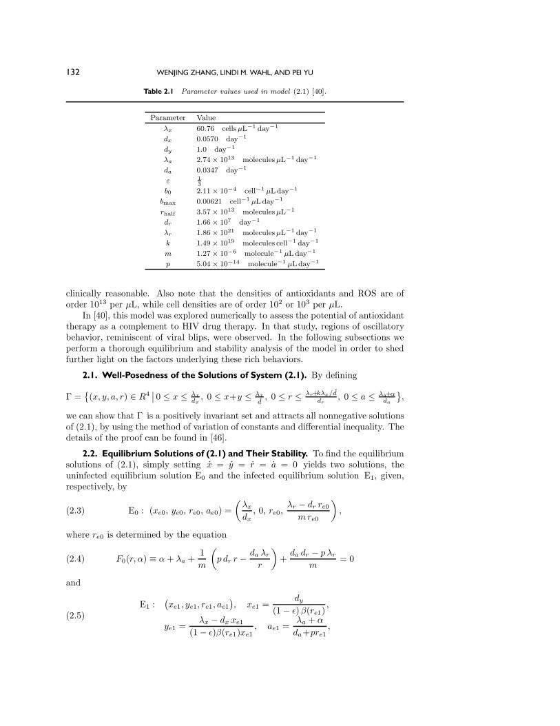
Table 2.1 Parameter values used in model (2.1) [40].

Parameter Value

λx 60.76 cellsμL−1 day−1

dx 0.0570 day−1

dy 1.0 day−1

λa 2.74× 1013 moleculesμL−1 day−1

da 0.0347 day−1

ε 13

b0 2.11× 10−4 cell−1 μLday−1

bmax 0.00621 cell−1 μLday−1

rhalf 3.57× 1013 moleculesμL−1

dr 1.66× 107 day−1

λr 1.86× 1021 moleculesμL−1 day−1

k 1.49× 1019 molecules cell−1 day−1

m 1.27× 10−6 molecule−1 μL day−1

p 5.04× 10−14 molecule−1 μLday−1

clinically reasonable. Also note that the densities of antioxidants and ROS are oforder 1013 per μL, while cell densities are of order 102 or 103 per μL.

In [40], this model was explored numerically to assess the potential of antioxidanttherapy as a complement to HIV drug therapy. In that study, regions of oscillatorybehavior, reminiscent of viral blips, were observed. In the following subsections weperform a thorough equilibrium and stability analysis of the model in order to shedfurther light on the factors underlying these rich behaviors.

2.1. Well-Posedness of the Solutions of System (2.1). By defining

Γ ={(x, y, a, r) ∈ R4

∣∣ 0 ≤ x ≤ λx

dx, 0 ≤ x+y ≤ λx

d, 0 ≤ r ≤ λr+kλx/d

dr, 0 ≤ a ≤ λa+α

da

},

we can show that Γ is a positively invariant set and attracts all nonnegative solutionsof (2.1), by using the method of variation of constants and differential inequality. Thedetails of the proof can be found in [46].

2.2. Equilibrium Solutions of (2.1) and Their Stability. To find the equilibriumsolutions of (2.1), simply setting x = y = r = a = 0 yields two solutions, theuninfected equilibrium solution E0 and the infected equilibrium solution E1, given,respectively, by

(2.3) E0 : (xe0, ye0, re0, ae0) =

(λx

dx, 0, re0,

λr − dr re0mre0

),

where re0 is determined by the equation

(2.4) F0(r, α) ≡ α+ λa +1

m

(p dr r −

da λr

r

)+

da dr − p λr

m= 0

and

(2.5)E1 :

(xe1, ye1, re1, ae1

), xe1 =

dy(1 − ε)β(re1)

,

ye1 =λx − dx xe1

(1− ε)β(re1)xe1, ae1 =

λa + α

da+pre1,


reacti

ve ox

ygen

spec

ies (r

)

1 20 3 4 5 6 7 81013

123456789

101013

antioxidant supplementation rate (α)

TranscriticalTurning

Hopf

Fig. 2.1 Bifurcation diagram for the 4-dimensional HIV antioxidant-therapy model (2.1) projectedon the r-α plane, restricted to the first quadrant, with the red and blue lines denoting E0

and E1, and the dashed and solid lines indicating unstable and stable, respectively.

where re1 is a function in the system parameters, particularly α (see the function F1

in 2.8)). Both E0 and E1 are expressed in terms of r (re0 or re1) for convenience.We first consider the uninfected equilibrium E0. The solution of re0 is determined

by (2.4), which is a quadratic equation in r. To simplify the analysis, we use r toexpress the parameter α since (2.4) is linear in α, and α is treated as a bifurcationparameter. Thus, solving F0(r, α) = 0 for α, we obtain

(2.6) α0(re0) = −λa −1

m

(p dr re0 −

da λr

re0

)− da dr − p λr

m.

To find the stability of the equilibrium solution E0, we first evaluate the Ja-cobian of system (2.1) at E0 to get J0(re0), where (2.6) has been used, and thenwe use det(ξ I − J0) to obtain the fourth-degree characteristic polynomial given byP0(ξ, re0) = (ξ + dx)

[ξ2 + (pre0 + da +

λr

re0)ξ + (daλr

re0+ pdrre0)

](ξ + P0r), where

(2.7) P0r = dy −(1− ε)λx(b0rhalf + re0bmax)

dx(re0 + rhalf).

P0(ξ, re0) contains three factors: the first is a linear polynomial of ξ, the secondis a quadratic polynomial of ξ, and both are stable polynomials (i.e., their roots(eigenvalues) have negative real part); thus the stability of E0 depends only on thethird factor, a linear polynomial of ξ. Therefore, when P0r > 0 (P0r < 0), theequilibrium solution E0 is asymptotically stable (unstable).

The bifurcation diagram for system (2.4) is shown in Figure 2.1, where only thepart in the first quadrant is depicted. The graph for the equation F0(r, α) = 0 givenin (2.4) is shown as the red line in Figure 2.1, which clearly shows a hyperbola. It isseen from this red line that the relation (2.4) also defines a single-valued function rin α. More precisely, it can be shown that the biologically meaningful solutions mustbe located on the first quadrant and above, including the red line, since E0 has thecomponent ye0 = 0.


Next, consider the infected equilibrium solution E1. The solution of re1 can besimilarly obtained by solving for r from the equation

(2.8) F1(r, α) = λr +kλx

dy− kdx(r + rhalf)

(1 − ε)(b0rhalf + bmaxr)− mr(λa + α)

pr + da− drr = 0,

which is again a linear function of α, and we can use re1 to express α as

α1(re1) = −λa +λr(pre1 + da)

mre1+

kλx(pre1 + da)

mre1dy

− kdx(re1 + rhalf)(pre1 + da)

mre1(1− ε)(b0rhalf + bmaxre1)− (pre1 + da)dr

m.(2.9)

The graph of the equations F0(r, α) = 0 given in (2.4) and F1(r, α) = 0 given in(2.8) is shown in Figure 2.1. To find the stability of E1, in a similar way, we evaluatethe Jacobian of (2.1) at E1 to obtain the fourth-degree characteristic polynomial,P1(ξ, re1)=ξ4+a1(re1)ξ

3+a2(re1)ξ2+a3(re1)ξ+a4(re1), where the lengthy expressions

for the coefficients a1 through a4 are omitted here for brevity.

2.3. Bifurcation Analysis. To understand the conditions underlying oscillatorybehavior and viral blips in this model, we now consider possible bifurcations whichmay occur from the equilibrium solutions E0 and E1.

2.3.1. Transcritical Bifurcation. First, for the uninfected equilibrium E0, it fol-lows from P0(ξ, re0) and (2.7) that in general E0 is stable for P0r > 0, and the onlypossible singularity occurs at the critical point, determined by P0r = 0 (see (2.7)).At this point, one eigenvalue of the characteristic polynomial becomes zero (and theother three eigenvalues still have negative real part), leading to a static bifurcation,and E0 becomes unstable. More precisely, when the parameter values in Table 2.1 areused, the two equilibrium solutions E0 and E1 intersect and exchange their stabilityat the point

(rt, αt

)≈ (8.89×1012, 4.58×1013), indicating that a transcritical bifur-

cation occurs at this critical point (see Figure 2.1). Here, the subscript “t” standsfor transcritical bifurcation. The value of αt is obtained by substituting rt into eitherα0(rt) in (2.6) or α1(rt) in (2.9). In fact, α0(rt) = α1(rt).

As discussed above, biologically meaningful solutions should be above or on theuninfected equilibrium solution E0 (the red line shown in Figure 2.1), since solutionsbelow the red line contain the component y < 0. The above discussion indicatesthat the uninfected equilibrium E0 is asymptotically stable (unstable) when r < rt(r > rt) or α > αt (α < αt) (see Figure 2.1), leading to the conclusion that no Hopfbifurcation exists on E0.

It should also be noted from Figure 2.1 that, besides a transcritical bifurca-tion point, E1 has a saddle-node bifurcation which occurs at the so-called turning

point. To determine this turning point, using (2.9) and dα1(r)dr = 0 yields (rs, αs)≈(

1.72×1013, 5.06×1013), where the subscript “s” denotes saddle-node bifurcation, and

αs=α1(rs) by using (2.9). Note that this bifurcation does not change the stability ofE1 since the characteristic polynomial P1(ξ, re1) still has an eigenvalue with positivereal part when re1 (or α) is varied along E1 to pass through the turning point (seeFigure 2.1), where a saddle-node bifurcation occurs. This can be seen more clearlyby examining the local dynamics close to the turning point on the center manifold;interested readers can find this detailed analysis in [46].


2.3.2. Hopf Bifurcation and Limit Cycles. To find any possible Hopf bifurca-tion which may occur from the infected equilibrium E1, we first need to determinethe critical points at which Hopf bifurcation occurs. The necessary and sufficientconditions for general n-dimensional systems to have a Hopf bifurcation are obtainedin [44]. When the parameter values in Table 2.1 are used, the critical values are givenby (rH , αH)≈(6.72×1013, 2.64×1013).

To find the approximate solutions of the limit cycles and to determine their stabil-ity, we apply normal form theory to the model associated with this singularity. First,we apply a transformation (x, y, r, a)T = (xe1, ye1, re1, ae1)

T + TH (x1, x2, x3, x4)T ,

where (xe1, ye1, re1, ae1) is the infected equilibrium solution E1 and TH is a constant,nonsingular matrix. We obtain a transformed system of (2.1), which we omit due toits lengthy expression. Then, applying the formulas of the normal form given in [45],we obtain

(2.10) ρ = ρ(v0 μ+ v1 ρ

2 + · · ·), θ = ωc + t0 μ+ t1 ρ

2 + · · · ,

where μ = α − αH , and ρ and θ denote the amplitude and phase of motion, re-spectively; ωc comes from the pure imaginary eigenvalues ±iωc at the Hopf criticalpoint. Then the first equation of (2.10) can be used to approximate the amplitudeof bifurcating limit cycles and to determine their stability. The second equation of(2.10) can determine the frequency of periodic motion. The coefficient v1, usuallycalled the first-order focus value, plays an important role in determining the stabilityof limit cycles. When v1 < 0 (v1 > 0, respectively), the Hopf bifurcation is calledsupercritical (subcritical) and the bifurcating limit cycles are stable (unstable). Forthe transformed system of (2.1) at the Hopf critical point, we obtain v0≈3.15 × 10−15

and t0≈3.33 × 10−15. Further, we apply the Maple program [43] to the transformedsystem to obtain v1≈−4.18×10−7 and t1≈−3.38×10−6. Thus, the normal form upto third order is given by

(2.11)ρ ≈ ρ(3.15×10−15μ− 4.18×10−7ρ2 + · · · ),θ ≈ 0.308+3.33×10−15μ−3.38×10−6ρ2+· · · .

Now, setting ρ = 0 results in two solutions: ρ = 0, which represents the infectedequilibrium solution E1, and ρ ≈ 8.68×10−5√μ (μ > 0), which is an approximationof the amplitude of bifurcating limit cycles. Since v1 < 0, this is a supercriticalHopf bifurcation, and bifurcating limit cycles are stable. For example, choosing μ =1012, we obtain the amplitude approximation of the limit cycle as ρ ≈ 86.8, and thefrequency of the limit cycle approximately as ω ≈ 0.283, slightly less than ωc ≈ 0.308.The phase portrait of the simulated limit cycle, projected on the x-y plane, is shown inFigure 2.2(d). It can be seen from Figures 2.2(a) and (d) that the analytical predictionfrom the normal form, ρ ≈ 86.8, agrees well with the simulated result.

The above analysis based on normal form theory is for local dynamical behavior;that is, the limit cycles must be near the Hopf critical point (rH , αH). It can beseen from Figure 2.1 that values of α taken from the interval α ∈ (αH , αt) lead tounstable equilibrium solutions (since both E0 and E1 are unstable for this interval).However, due to the solutions being nonnegative and bounded, we expect that thereshould exist certain persistent motions such as oscillating solutions for the values ofα taken from this interval, and the amplitudes of these oscillations can be large. Forexample, for α = 3.50× 1013, the phase portrait of the simulated solution, projectedon the x-y plane, is shown in Figure 2.2(e), corresponding to the oscillations in time


0 100 200 300 400 5000

100

200

300

400

500

600

Day

(a)

0 100 200 300 4000

200

400

600

800

Day

(b)

0 500 1000 15000

200

400

600

800

1000

1200

Day

(c)

200 300 400 5000

20

40

60

80

100

x

y

(d)

100 300 500 7000

50

100

150

200

250

x

y

(e)

0 200 400 600 800 1000 12000

50

100

150

200

250

300

x

y

(f)

Fig. 2.2 Simulated limit cycles of system (2.1) for the parameter values taken from Table 2.1, withthe time course of x (blue) and y (red) on the top row and the corresponding phase portraitsprojected on the x-y plane on the bottom row. For (a) and (d) α = 2.74 × 1013, for (b)and (e) α = 3.50× 1013, and for (c) and (f) α = 4.55× 1013.

shown in Figure 2.2(b), which have much greater amplitude than the oscillations inFigure 2.2(a).

Now, we take a particular value of α from the interval α ∈ (αH , αt), which is closeto αt, to simulate the system. For example, taking α=4.55×1013<αt≈4.58×1013, weobtain the phase portrait of the simulated oscillating solution, projected on the x-yplane, shown in Figure 2.2(f), with the corresponding time history of x and y shownin Figure 2.2(c). This clearly shows viral blips.

Next, we will discuss what conditions are needed for creating the phenomenon ofviral blips.

2.4. Conditions for Generating Viral Blips. In the previous subsection, we care-fully analyzed the occurrence of viral blips in a 4-dimensional HIV model (2.1). Sys-tem (2.1) is an example of an in-host infection model, an ODE system describing thedynamics of infection within a single infected individual. In-host infection models,based on classical susceptible-infected-recovered (SIR) models in epidemiology [1],typically include populations of uninfected target cells, infected target cells, and theinfection dynamics between the two classes [29]. More complex models also includepopulations of free virus, latently infected cells, and various relevant components ofthe immune response, depending on the infection under study. Although there aremany exceptional cases, in-host models typically admit an uninfected equilibrium andat least one infected equilibrium, analogous to the disease-free and endemic equilibriaof an SIR model.

Since in-host infection models share many similar features, much of our under-standing regarding the behavior of system (2.1) can be generalized to other models.


Based on insights obtained in analyzing system (2.1), we propose in the followinghypothesis four conditions for an in-host infection model to generate viral blips.

Hypothesis 1. The following conditions are needed for an in-host infection modelto generate viral blips:

(i) there exist at least two equilibrium solutions;(ii) there exists a transcritical bifurcation at an intersection of the two equilibrium

solutions;(iii) there is a Hopf bifurcation which occurs from one of the equilibrium solutions;

and(iv) large oscillations (or, more generally, global, persistent motions) can occur

near the transcritical critical point.The reasons for conditions (i) and (ii) are simple because when a parameter that

reflects infection severity is chosen as a bifurcation parameter, an in-host infectionmodel typically starts at the uninfected equilibrium and then bifurcates to the infectedequilibrium as the parameter is increased. Thus, these two equilibrium solutions mustexchange their stability, yielding a transcritical bifurcation. For the 4-dimensionalmodel considered in the previous subsection, the uninfected equilibrium E0 and theinfected equilibrium E1 intersect at the critical point (αt, rt), where they exchangetheir stability. In fact, E0 is stable (unstable) for α > αt (α < αt), while the lowerbranch of E1 is stable (unstable) for α < αt (α > αt), as shown in Figure 2.1.

Condition (iii), the existence of a Hopf bifurcation, is necessary to obtain oscilla-tions. It can be seen from Figure 2.1 that limit cycles bifurcate from E1 at the Hopfcritical point (αH , rH), and they become larger if μ = α− αH > 0 increases.

The reasoning behind condition (iv) is not so obvious. Large oscillations (orglobal, persistent motions) are necessary, near the transcritical point, for viral blipsto emerge. As shown in Figure 2.1, both E0 and E1 are unstable for α ∈ (αH , αt)(though a part of the lower branch of E1 is stable, it is biologically meaningless sincey < 0). Thus, there exist large oscillations near the transcritical critical point αt.Moreover, it is noted from Figure 2.1 that at the left side of the transcritical pointαt, the eigenvalues evaluated at E0 are all real, containing one positive eigenvalue(ξ01 > 0) and three negative eigenvalues (ξ0i < 0, i = 2, 3, 4). In other words, any pointon the uninfected equilibrium E0 for α < αt is a saddle point. Since ξ01 crosses zero atthe critical point α = αt, it is very small near the transcritical point for α < αt. Onthe other hand, the infected equilibrium E1 is an unstable focus-type point since theeigenvalues at E1 contain a complex conjugate pair with positive real part and twonegative real eigenvalues (see Figure 2.1). Now, we need to answer two questions: (1)Where does the large periodic solution (limit cycle) come from? (2) Why does theperiodic solution contain a region of very fast motion and a region of very slow motion?

To answer the first question, see from Figure 2.2(f) that since there exists a saddlepoint outside the stable limit cycle and the stable limit cycle encloses an unstablesingular point, there may exist an unstable homoclinic orbit which passes through thesaddle point and encloses the stable limit cycle. The possible homoclinic orbit andthe limit cycle can be thought of as being embedded in a 2-dimensional submanifold.However, this possibility can be ruled out as follows: Suppose there exists a homoclinicorbit embedded in a 2-dimensional submanifold. Then this homoclinic orbit muststart from E0 (the saddle point) and return to the same point. First note that all theeigenvalues at this saddle point are real (see Figure 2.1), and one of them is −dx. Itcan be shown that the eigenvector associated with this eigenvalue is (1, 0, 0, 0), i.e., inthe direction of the x-axis. Now consider the line in the 4-dimensional space, throughthe two points (x, y, r, a) = (0, 0, re0, ae0) and (x, y, r, a) = (xe0, 0, re0, ae0), and call


0

50

100

150

200

250

300

350

0 200 400 600 800 1000 1200

y

x

E

E

1

00.003

0.096.517

3870

102

161

267

381

321191

134

107

84

64

51

42

41

4139 31 26 21 15 9.5

8.0 6.5 5.0 3.7 2.3 0.9 0.03

��

�

�

�

� �

Fig. 2.3 Simulated blips projected on the x-y plane. Labels along the solution curve reflect therelative speed of the trajectory at each point.

the line segment between the two points S∗. It is easy to see that this line passesthrough the equilibrium solution (the saddle point) E0 and is in the direction of theeigenvector (1, 0, 0, 0). Moreover, it can be shown by using (2.1) that this line itselfis actually a solution trajectory of the system (an invariant manifold of the system).This implies that if a homoclinic orbit passing through the saddle point E0 exists, itmust return to the saddle point E0 along S∗. In other words, S∗ must be a part of thehomoclinic orbit. But this is impossible because S∗ does not contain singular pointsfor x ∈ [0, xe0) and thus no other possible trajectories can connect this particulartrajectory S∗ due to the uniqueness of solutions. This will be seen more clearly laterwhen we discuss the 2-dimensional model in section 4.

To answer the second question and make the answer more clear, we consider avalue of α < αt, but near the critical point α = αt (e.g., α = 4.55 × 1013, as shownin Figures 2.2(c) and (f)). For simplicity, we consider the projection of the solutiontrajectory for this case on the x-y plane, as depicted in Figure 2.3, where the twoequilibrium points E0 and E1 are shown. Due to 0 < ξ01 � 1, it is expected thatthe trajectory moves very slowly near the saddle point E0, while it moves rapidlywhen it is away from this point. In fact, we have shown in Figure 2.3 the speed ofthe trajectory along the solution curve (limit cycle). It can be seen from this figurethat the speed indeed varies from very small (near the saddle point), on the order of3 × 10−3, to very large (away from the saddle point), on the order of 3 × 102. Thus,the small part in the phase portrait with very slow speed actually takes a longer time,while the large part in the phase portrait with very fast speed takes much less time, asshown in the time history (see Figure 2.2(c)). This fast-slow motion yields the blipsphenomenon, with slow changes corresponding to the near-flat section in the timehistory, and rapid changes occurring during the viral blips, as shown in Figures 2.2(c)and (f). In other words, the trajectory spends relatively long periods in regions ofstate space which lie very close to the uninfected equilibrium and then transientlyvisits regions of state space which are close to the infected equilibrium.


3. A Simple 3-Dimensional In-Host Infection Model Producing Blips. Havingestablished the conditions in Hypothesis 1 for generating viral blips, we are ready toturn to some basic questions such as the following: What types of in-host infectionmodels can generate blips, and what is the minimum dimension of such models?

3.1. Generalizing ROS to Other Physical Variables. In model (2.1), the vari-able r represents ROS, which are produced naturally in the body. In HIV infection,extra ROS are generated by infected cells, and these in turn directly accelerate HIVprogression [30, 37]. Therefore, infectivity β is an increasing and saturating functionof ROS concentrations. However, we note that the form of the infection term is notspecific to HIV or to ROS, and models of a similar form could in fact apply to otherinfections. To generalize the physical meaning of the variable r, we can, for exam-ple, let r denote any damage caused by the infection to, for example, the humoralimmune response, the infected organs, or the infected individual aspecifically. Themodel assumes that “damage” increases with the extent of the infection at rate kyand is repaired or cleared at rate drr. This yields the 3-dimensional system

(3.1) x = λx − dxx− β(r)xy, y = β(r)xy − dyy, r = ky − drr.

To achieve an infection term similar to that in model (2.1), we further assume thataccrued damage makes target cells more vulnerable to infection, that is, accrueddamage increases the infection rate. We thus take β(r) to be an increasing, saturatingfunction of r.

In the original model (2.1), r represents ROS, for example, H2O2, whose produc-tion and decay rates are both extremely fast. For the more general model (3.1), wewould like to assess whether viral blips are still possible at more moderate productionand repair rates, k and dr. For ROS the decay rate dr =1.66 ×107 day−1 implies ahalf life of only 4ms. We decreased dr by several orders of magnitude and found that,in particular, at dr = 1.0×103 day−1, a half life of 60s, viral blips are still possible.For this value of dr, we can take k=1.49×1015molecules cell−1 day−1. Note that λr

has been set to zero in (3.1) to make the model more general.For simplicity, let a = bmax−b0, b = b0, and c = rhalf . Then the function β(r)

is rewritten as β(r) = b+ a rr+c , and a, b, and c are treated as bifurcation parameters.

Parameter values λx, dx, dy, k, dr, b0, bmax, and rhalf are given in Table 2.1. For prac-tically meaningful solutions, the values of the bifurcation parameters will be chosenclose to the values in Table 2.1.

To analyze (3.1), we can follow the same procedure used in the previous sectionand treat b as a bifurcation parameter. First, it is easy to prove the well-posednessof system (3.1). Next, we get the infection-free equilibrium E0 : (xe0, ye0, re0) =

(λx

dx, 0, 0) and the infected equilibrium E1 := (xe1, ye1, re1), where xe1=

dy(re1+c)(a+b)re1+bc ,

ye1=1dy(λx−dxxe1), and re1 is determined by F1(r, c) = drdy(a+b)r

2+[dy(drbc+kdx)−kλx(a+b)] r+kc(dxdy−bλx) = 0. Again, it is easy to show that E0 and E1 intersect atthe transcritical bifurcation point (bt, rt) ≈ (9.38×10−4, 0). On the infected equilib-rium E1, there is a saddle-node bifurcation point (turning point) (bs, rs) ≈ (−1.49×10−3, 4.18×1013) and a Hopf bifurcation point (bH , rH) ≈ (6.56×10−4, 7.24×1013).

The bifurcation diagram and simulated results are shown in Figure 3.1. All theconditions (i)–(iv) in Hypothesis 1 are satisfied. Blips do appear since the Hopfcritical point is close to the transcritical point. However, because E1 is not globallystable, depending on the initial conditions, the oscillation may converge to the stableequilibrium E1 (see Figure 3.1(b)) or converge to a limit cycle with large amplitude


Turningr

b(a)

0 100 200 300 400 50035

40

45

50

55

60

65

Day

y

(b)

0 100 200 300 400 5000

100

300

500

700

y

Day(c)

Fig. 3.1 Dynamics and bifurcation of system (3.1) for dr=1.0×103, k=1.49×1015: (a) bifurcationdiagram projected on the b-r plane; (b) simulated time history y(t) converging to E1 forb = 0.001 with the initial condition (x, y, r) = (178, 46, 73) close to E1; and (c) simulatedtime history y(t) converging to a stable limit cycle (blips) for b = 0.001 with the initialcondition (x, y, r)=(1005, 3, 3) close to E0.

(blips), as shown in Figure 3.1(c). Convergence to a smaller, regular oscillation dueto the Hopf bifurcation is also possible (not shown in Figure 3.1). Similarly, followingthe discussion in the previous section for the 4-dimensional model, we can show thatthe existence of the blips (limit cycle) is not due to homoclinic bifurcation. In fact,no homoclinic orbits can exist.

3.2. Identifying the Region of Parameter Space Exhibiting Viral Blips. Hav-ing found viral blip behavior in the simple 3-dimensional infection model (3.1), we arenow further interested in identifying the region of parameter space in which viral blipsmay occur. This is particularly useful in applications since, in reality, all parametersare roughly measured. Thus, we need to study the robustness of the phenomenonto variations in the system parameters. If blips appear only for a very small regionin the parameter space, then the results are not practically useful. The main idea ofidentifying the region where blips may occur is to study the instability of the solutionsof the system. Once the unstable region is identified, blips can be found by using theother conditions in Hypothesis 1. In order to simplify the analysis, we first introducestate variable scaling and parameter rescaling into system (3.1).

3.2.1. State Variable Scaling and Parameter Rescaling. Introducing the scal-ing x= c1X, y= c2Y, r= c3R, t= c4τ , where c1=

λx

dy, c2=

λx

dy, c3=

λxk1012d2

y, c4=

1dy, to

(3.1) and letting A = aλx

d2y, B = b λx

d2y, C =

c d2y

λxk, Dx = dx

dy, Dr = dr

dyyields the scaled

system(3.2)dX

dτ= 1−DxX−

(B +

AR

R+C

)XY,

dY

dτ=

(B +

AR

R+C

)XY −Y,

dR

dτ= Y −DrR,

which will be used in the following analysis, with the scaled parameter values givenby

(3.3) A = 0.364, C = 3.94× 10−4, Dx = 0.057, Dr = 1000

and with B treated as a bifurcation parameter.

3.2.2. Equilibrium Solutions and Their Stability. The bifurcation patterns ofthe scaled system (3.2) are the same as those of system (3.1). Two equilibrium


(a)

C

B

(b)

A

B(c)

Fig. 3.2 (a) Graph of Δ2 = 0 in the A-B-C parameter space, identifying the region yielding oscilla-tions; (b) cross section of panel (a), where A = 0.364; and (c) cross section of panel (a),where C=3.94×10−4.

solutions are E0 : (Xe0, Ye0, Re0) = ( 1Dx

, 0, 0) and E1 : (Xe1, Ye1, Re1), where Xe1 =Re1+C

(A+B)Re1+BC , Ye1 = DrRe1, and Re1 is determined from the equation F3(R) =

Dr(A+B)R2+[Dr +BC+Dx−(A+B)]R+(Dr−B)C=0.The characteristic polynomial for E0 is P0(ξ) = (ξ + Dx) (ξ + Dr) (ξ − B

Dx). It

is easy to show that E0 and E1 exchange stability at the transcritical bifurcationpoint B = Dx. The characteristic polynomial for E1 is P1(ξ, re1) = ξ3 + a1(re1)ξ

2 +a2(re1)ξ+a3(re1), and the Hopf critical point is determined by Δ2 = a1(re1) a2(re1)−a3(re1) = 0. We fix parameters Dr and Dx and choose A, B, and C as bifurcationparameters. Then we want to find the parameter region where blips may occur. First,a Hopf bifurcation is necessary, requiring the condition Δ2(A,B,C) = 0. The graphof Δ2(A,B,C)=0 is plotted in the 3-dimensional A-B-C parameter space, as shownin Figure 3.2(a), where the green hypersurface defines a set of points which are Hopfcritical points; the region bounded by the green surface is unstable for E1, leadingto oscillations. Thus blips may occur within this region and near the boundary aswell, depending on the relative position of the Hopf critical point with respect to thetranscritical point.

In the following, we fix either parameter A or parameter C to enable the anal-ysis and obtain 2-dimensional graphs, which illustrate more clearly the bifurcationsnecessary for blips.

3.2.3. Parameter A Fixed. Fix A = 0.364, which cuts the surface in Figure 3.2(a)to yield curves, as shown in Figure 3.2(b). The transcritical bifurcation occurs atB = 0.057, which is denoted by a red line in Figure 3.2(b). A Hopf bifurcation occurson the green curve, and the region bounded by the green and red curves indicateswhere oscillations can happen. It should be noted that the above results are basedon local dynamical analysis; thus blips may also appear outside this bounded regionbut close to the green curve.

We take three typical values of C (as the three dotted lines shown in Figure 3.2(b)),and we obtain the Hopf critical points as follows:

(3.4)

C = 0.002 : (BH , RH) ≈ (1.69×10−1, 7.90×10−4),C = 0.012 : (BH1 , RH1) ≈ (6.27×10−2, 1.53×10−4),C = 0.012 : (BH2 , RH2) ≈ (1.06×10−1, 5.31×10−4),C = 0.018 : No Hopf critical point.


The bifurcation diagrams corresponding to the three lines C =0.002, C =0.012,and C=0.018 are shown in the top three graphs in Figure 3.3. Six simulated resultsare also presented in this figure, corresponding to the six points marked on the threedotted lines in Figure 3.2(b). It can be seen that the values taken from the points(1)–(4) generate blips, point (5) leads to a regular oscillation, while point (6) gives asimple stable equilibrium solution, as expected. For this case when parameter A isfixed, no blips have been found for the values outside the region bounded by the redand green curves. It should be noted in the top middle figure of Figure 3.3 that thereare two Hopf bifurcation points on the equilibrium E1. One of them is supercritical,while the other is subcritical, but the two families of the limit cycles bifurcating fromthese two critical points are both stable, since the stability change is reversed at thetwo points. In fact, the three eigenvalues along the unstable part of E1 between thetwo Hopf bifurcation points contain one negative eigenvalue and a pair of complexconjugates with positive real part. On the two stable parts, the real part of thecomplex conjugate eigenvalues changes sign to become negative. As the parameter Cincreases from 0.002 to 0.018, the two Hopf bifurcation points merge to a single pointon E1 (corresponding to the turning point on the green curve (see Figure 3.2(b)), atwhich the horizontal line is tangent to the green curve); the corresponding eigenvaluescontain a negative eigenvalue and a purely imaginary pair. This indeed characterizes adegenerate Hopf bifurcation (see, e.g., [45]) different from the Hopf bifurcation definedby (2.10). A similar discussion applies to the other two Hopf bifurcation points shownin the top left panel in Figure 3.4.

3.2.4. Parameter C Fixed. Now we fix parameter C = 3.94×10−4, which resultsin curves in the A-B plane by cutting the surface in Figure 3.2(a), as shown inFigure 3.2(c). The transcritical point is kept the same: B = 0.057. We choose threetypical values of A and find the Hopf bifurcation points as follows:

(3.5)

A = 0.025 : (BH1 , RH1) ≈ (5.82×10−2, 9.84×10−5),A = 0.025 : (BH2 , RH2) ≈ (6.75×10−2, 2.65×10−4),A = 0.200 : (BH , RH) ≈ (8.32×10−2, 7.33×10−4),A = 0.364 : (BH , RH) ≈ (3.99×10−2, 7.99×10−4).

The bifurcation diagrams corresponding to the three lines A=0.025, A=0.200,and A=0.364 are shown in the top three graphs in Figure 3.4. Nine simulated resultsare also presented in this figure, corresponding to the nine points marked on the fivedotted lines in Figure 3.2(c). It is observed from these graphs that among the ninechosen parameter values, seven cases exhibit blips (see the points (2)–(7) and (9) inFigure 3.2(c) with the corresponding simulated results shown in Figure 3.4). It isnoted that some of these points are not even close to the red line, nor are they in theregion bounded by the red and green curves, suggesting that a simple 3-dimensionalHIV model can generate rich blips.

3.3. A 3-Dimensional Immunological Model. In this subsection, we briefly con-sider an immunological model [29] and apply Hypothesis 1 to show that the model canhave blips. For simplicity, the original 4-dimensional model [4] is reduced (by a quasi-steady-state assumption on the virus particles) to a 3-dimensional model, describedby

(3.6) x = λ− dx− β(y)xy, y = β(y)xy − ay − pyz, z = cyz − bz,

where x, y, and z represent the densities of the uninfected cells, infected cells, andcytotoxic T lymphocytes (CTLs), respectively. The system (3.6) with constant β(y)


R

B

R

B

R

B

0 200 400 600 800 1000 12000

100

200

300

400

500

600

700

Day

y

(1)

0 50 100 150 2000

100

200

300

400

500

600

700

Day

y

(2)

0 20 40 60 80 100 1200

50

150

250

350

450

550

Day

y

(3)

0

40

80

120

160

200

Day

y

(4)

0 100 200 300 400 5000

40

80

120

160

200

Day

y

(5)

0 200 400 600 800 1000 12000

50

100

150

200

250

300

Day

y

(6)

Fig. 3.3 Bifurcation diagrams corresponding to C = 0.002, 0.012, and 0.018, respectively,and numerical simulation results for the parameter values (B,C) = (0.06, 0.002)(1),(0.08, 0.002)(2), (0.10, 0.002)(3), (0.07, 0.012)(4), (0.09, 0.012)(5), (0.08, 0.018)(6).

is well known [7, 28] and does not exhibit blips. In order to generate viral blips, herewe choose β(y) = n+ my

y+k , where n and m are minimum and maximum infectivity,and k represents the density of infected cells when the infectivity takes its medianvalue. Since the analysis is similar to previous models, we omit the details and giveonly the results as follows. The system (3.6) has three equilibrium solutions: theinfection-free equilibrium, E0, the infected equilibrium with CTL, E1, and the in-fected equilibrium without CTL, E2. There are two transcritical bifurcation points.One, named “Transcritical 1” in Figure 3.5(a), is at the intersection of E0 and E2:(nt1, yt1) ≈ (0.005, 0), at which E0 and E2 exchange their stability. The second oc-curs at the intersection of E1 and E2: (nt2, yt2) ≈ (−0.01, 0.5), called “Transcritical2” in Figure 3.5(a). However, note that they only exchange their stability if restrictedto a 1-dimensional manifold, and both are unstable in the whole space since one of theeigenvalues stays positive when crossing this transcritical point. E1 becomes stableuntil n is increased to cross a Hopf critical point (called “Hopf 1” in Figure 3.5(a)):(n1H , y1H) ≈ (0.206, 0.5). Another Hopf bifurcation point (called “Hopf 2” in Fig-ure 3.5(a)) happens on E2 at (n2H , y2H) ≈ (0.0213, 1.81). It should be noted that


R

B R

B

Hopf

R

B

0 100 200 300 400 500 600

0

10

20

30

40

50

60

Days

y

(1)

0 200 400 600 800 10000

100

200

300

400

500

600

Day

y

(2)

0 100 200 300 4000

100

200

300

400

500

600

Day

y

(3)

0 50 100 150 2000

100

200

300

400

500

600

Day

y

(4)

0 200 400 600 800 10000

100

200

300

400

500

600

700

Day

y

(5)

0 100 200 3000

100

200

300

400

500

600

700

Day

y

(6)

0 100 200 300 400 500 600 700 8000

100

200

300

400

500

600

700

800

Day

y

(7)

0 100 200 300 400 5000

100

200

300

400

500

600

Day

y

(8)

0 100 200 300 400 500 600 7000

100

200

300

400

500

600

700

800

Day

y

(9)

Fig. 3.4 Bifurcation diagrams corresponding to A=0.025, 0.200, 0.364 and numerical simulation re-sults for the parameter values (A,B)=(0.025, 0.060)(1), (0.200, 0.060)(2), (0.200, 0.070)(3),(0.200, 0.085)(4), (0.300, 0.059)(5), (0.300, 0.070)(6), (0.364, 0.060)(7), (0.364, 0.070)(8),(0.400, 0.060)(9).

this Hopf bifurcation occurs from a 2-dimensional manifold that is orthogonal to a 1-dimensional unstable manifold. That’s why the E2 stays unstable when the parameteris varied to pass through this Hopf critical point. The limit cycles bifurcating from“Hopf 1” are stable, while those from “Hopf 2” are unstable, leading to large oscillat-ing motions when the values of n are chosen near the two singular points “transcritical


Transcritical 2

Transcritical 1

Hopf 2

Hopf 1

E2

E0

E1

(a)

0 50 100 150 200 250 3000

5

10

15

20

25

Day

y

(b)

Fig. 3.5 (a) Bifurcation diagram of system (3.6), showing the equilibrium solutions E0, E1, and E2

with dashed and solid lines denoting unstable and stable, respectively. (b) Simulated viralblips in system (3.6) for n = 0.04. Other parameter values used here are λ=k=p=1, d=0.01, m=b=0.05, a=0.5, c=0.1.

1” and “Hopf 2.” The above results show that all four conditions in Hypothesis 1 aresatisfied, and blips indeed appear. The simulated blips for n = 0.04 are depicted inFigure 3.5(b).

4. A 2-Dimensional In-Host Infection Model. For the generalized 3-dimensionalmodel discussed in section 3, we assume that r is some form of damage to the hostor to the host immune system that increases with the extent of the infection, thatis, in proportion to the infected cell density. Here, we further assume that there isa quasi-steady state (as used in (3.1)) between the damage r and the infected cell y.Thus, the 3-dimensional HIV model can be further reduced to a 2-dimensional model,given by

(4.1) x = λx − dxx− β(y)xy, y = β(y)xy − dyy.

Note that system (4.1) is now in the form of an in-host infection model, which includesonly uninfected and infected target cell populations and the most basic “birth” anddeath rates. However, we now think of the infectivity β(y) as a possible function of y;other parameters have the same meaning as in (3.6). We will show that this simplified2-dimensional infection model may also be able to generate blips.

4.1. A 2-Dimensional In-Host Model with Constant and Linear InfectionRates. First, we consider the case when the infection rate, β(y), is simply a con-stant function; that is, β(y) = β. Taking β itself as a bifurcation parameter, it iseasy to show that there exist two equilibrium solutions and a transcritical bifurcationpoint, but no Hopf bifurcation exists. This violates Hypothesis 1, and therefore noblips can appear in this case.

Next, suppose the infection rate β(y) is a linear function of the infected celldensity, y, that is, β(y) = b + ay, where the parameters a and b represent the sameconstants as before and a is treated as a bifurcation parameter. In this case, we havetwo equilibrium solutions E0 and E1. But E0 is always stable for all values of a thoughthere exists a Hopf bifurcation on E1. Therefore, no transcritical bifurcation pointexists for this case, which violates Hypothesis 1, implying that blips are not possiblewhen β(y) is a linear function.


4.2. A 2-Dimensional In-Host Model with Saturating Infection Rate. Moti-vated by our previous results for the 3- and 4-dimensional models, we next assumethat infectivity is an increasing saturating function of the infected cell density y,namely, β(y) = b+ ay

y+c . For our numerical work, we take the same values of a and bas used in section 3.1, while c is taken to be c = 50, obtained by numerical simulationbased on the experimental data given in [40]. Other parameter values are as describedfor model (3.1).

4.2.1. Scaling. For convenience in the following analysis, we first simplify sys-tem (4.1) by the following scaling to reduce the number of parameters. Let x =e1X, y= e2Y, t= e3τ , where e1=

λx

dy, e2=

λx

dy, e3=

1dy, and set A= aλx

d2y, B= λxb

d2y, C=

cdy

λx, D= dx

dy. Then the rescaled system is given by

(4.2)dX

dτ= 1−DX −

(B +

AY

Y + C

)XY,

dY

dτ=

(B +

AY

Y + C

)XY − Y,

with B treated as a bifurcation parameter. Taking the parameter values from [29],we have the scaled parameter values A=0.364, C =0.823, andD=0.057 for system(4.2).

4.2.2. Equilibrium Solutions and Their Stability. By setting X= Y =0 in (4.2),we get two biologically meaningful equilibrium solutions, the uninfected equilibriumsolution E0 : (X0, Y0) = ( 1

D , 0) and the infected equilibrium solution E1 = (X1, Y1),

where X1=Y1+C

(A+B)Y1+BC and Y1 is determined by the equation F1=(A+B)Y 2+(D+

BC−A−B)Y +(D−B)C = 0. This indicates that condition (i) in Hypothesis 1 issatisfied. Similarly, it is easy to find that E0 is stable (unstable) if B < D (B > D).

4.2.3. Bifurcation Analysis. By using the characteristic polynomials at E0 andE1, we can show that a transcritical bifurcation occurs at the critical point, (Yt, Bt) =(0, 0.057), which satisfies condition (ii) in Hypothesis 1. E0 and E1 intersect at thiscritical point and exchange their stability. Further, a Hopf bifurcation happens at thecritical point (BH , YH) ≈ (0.121, 0.811). E1 is stable (unstable) on the right (left)side of the Hopf bifurcation point. Therefore, condition (iii) in Hypothesis 1 holdsfor this case. If we take a value of B near Bt on the side where both E0 and E1

are unstable, then condition (iv) in Hypothesis 1 is also satisfied and so blips occur.The bifurcation diagram is shown in Figure 4.1(a), and the simulated viral blips forB = 0.060 are depicted in Figure 4.1(b).

For this 2-dimensional model, we study the blips phenomenon more carefully andrigorously show the existence of the blips. To achieve this, we plot the phase portrait,corresponding to the time history in Figure 4.1(b), as shown in Figure 4.2(a), whereE0 is a saddle point, with eigenvalues 0.0526, −0.057, and E1 is an unstable focus,with eigenvalues 0.0766 ± 0.3865i. Comparing Figure 4.2(a) with Figure 2.3 indeedshows that the qualitative behavior of the system does not change after the modelreduction from four dimensions to two dimensions, with only the value of y increasedin the 2-dimensional model. Note that we do not show the speed of the trajectory inFigure 4.2(a) since it is similar to that in Figure 2.3.

Now we want to show that no homoclinic orbits can exist for this model. First,it is easy to find that the two eigenvalues at the saddle point E0 are ξ1 = −D andξ2 = B

D − 1 (> 0 for B > D), and their corresponding eigenvectors are v1 = (1, 0)

and v2 = (1, DB (1 − D) − 1), respectively. It should be noted that for convenience

(x, y) are used in Figure 4.2(a), while (X,Y ) are used in Figure 4.2(b); their relation


Y

B(a)

0 200 400 600 8000

2

4

6

8

10

12

Day

Y

(b)

Fig. 4.1 (a) Bifurcation diagram projected on the B-Y plane, with the thick and thin lines denotingE0 and E1, respectively, and dotted and solid lines indicating unstable and stable, respec-tively. (b) Simulated time history of y(t) for B = 0.060.

0

100

200

300

400

500

600

700

0 200 400 600 800 1000 1200

y

x

E

E

1

0

�

�

�

�

�

�

�

� �� 1E

0E

X

Y

K = DB

(1−DB

)−1

0 17.54

16.71

(a) (b)

Fig. 4.2 (a) Simulated phase portrait of the blips (see Figure 4.1(b) for the time history). (b)Construction of the trapping region of the blips (limit cycle).

is given by (x, y) = (60.76X, 60.76Y ). The first eigenvector v1 is in the directionof the X-axis. Thus, if a homoclinic orbit exists, it must leave the saddle point E0

along the direction of v2 and return to the point along v1. Further, we can use (4.2)to show that the X-axis is actually a solution trajectory of this system. Thus, if ahomoclinic orbit passing through the saddle point E0 exists, it must contain the partof the X-axis from X = 0 to X = 1

D . However, this is impossible because this part ofthe X-axis for X ∈ [0, 1

D ) does not contain singular points and so no other trajectoriescan connect the X-axis for X ∈ [0, 1

D ) due to the uniqueness of solutions. Therefore,no homoclinic orbits can exist and thus the stable limit cycle (blips) is not due tohomoclinic bifurcation.

Next, we apply Poincare–Bendixson theory to prove the existence of the limitcycle. Since E1 is an unstable focus point, we can construct an annulus to form atrapping region, with the inner closed boundary, a circle with small enough radius,enclosing the focus point E1, and the outer boundary, a right triangle as shown in Fig-ure 4.2(b), consisting of the X-axis, the Y -axis, and the hypotenuse Y = K(X − 1

D ),


where K = DB (1− D

B )−1 is the slope of the hypotenuse. It is obvious that all solutiontrajectories inside the inner boundary move toward the trapping region, since E1 isan unstable focus. For the outer boundary, first note that the slope of the hypotenuseis less than that of the eigenvector v2, i.e., the hypotenuse stands more vertically thanv2. As has been shown above, the X-axis is a trajectory of the system. For the Y -axis,it is easy to see that for Y > 0, dX

dτ = 1, dYdτ = −Y < 0, implying that trajectories

cross the Y -axis in the left to right, downward direction (see Figure 4.2(b)). For thehypotenuse Y = K(X − 1

D ), X ∈ [0, 1D ), we can use the equation of the hypotenuse

and the differential equations in (4.2) to show that all trajectories cross the hypotenusein the direction toward the trapping region, as shown in Figure 4.2(b). Therefore, byapplying Poincare–Bendixson theory, we know that there exists at least one closedorbit (limit cycle) within this trapping region. The numerical simulation shows thatonly one closed orbit (limit cycle) exists within this trapping region. It is noted thatfor the given parameter values B = 0.06, D = 0.057, the two eigenvalues at the saddlepoint E0 are −0.06 and 0.053, associated with the eigenvectors v1 = (1, 0) (in the X-axis direction) and v2 = (1,−0.104), respectively (see Figure 4.2(b)). This is why thetrajectory moves very slowly around the corner of the saddle point E0, while it movesvery quickly when it is away from this corner. For example, at the point (X,Y ) =(6.641, 9.574) the eigenvalues are −1.020±1.625i, so the convergence rate at this pointto that of the point near the saddle point E0 is about 1.02

0.05 ≈ 20, showing that the tra-jectory moves through this point much faster than the points near the saddle point E0.

Summarizing the results of this section, we conclude that the simple 2-dimensionalin-host model is sufficiently complex to exhibit viral blips, provided the infectivityfunction is an increasing, saturating function of infected cell density. However, forthis model, the range of parameter space in which blips occur is relatively restricted,compared with the 3-dimensional model, which is established in the previous section.

An interesting question naturally arises: Does there exist a more general functionβ(y) such that the existence of blips depends upon the general properties of thefunction like its maximal values and/or its derivatives? In fact, it has been found thatby choosing the parameter c large enough in the function β, a threshold is reachedbeyond which the Hopf bifurcation and hence also the viral blips disappear.

5. Recurrency in a 5-Dimensional Model. So far, we have considered 2-, 3-, and4-dimensional in-host infection models with increasing, saturating, infectivity func-tions and have shown that all these models exhibit blips. Moreover, it has been shownfor the 2-dimensional model (and can be shown for the 3- and 4-dimensional models,though omitted here) that replacing the infectivity function with a constant or linearfunction of y will cause blips to disappear. However, in this section we will show thathigher-dimensional systems may have blips even with a constant infectivity function.

We consider a previously proposed 5-dimensional immunological model in whichrecurrent phenomena or viral blips have been observed via numerical simulation [42].The model describes antibody concentrations and CTLs explicitly and is described asfollows:

x = λ− dx− βxv,(5.1a)

y = βxv − ay − pyz,(5.1b)

z = cyz − bz + hy,(5.1c)

u = ξz − ηu− kuv,(5.1d)

v = ey − kuv − γxv − qv.(5.1e)

Here x, y, z, u, and v are, respectively, the population densities of uninfected targetcells, infected target cells, CTLs, antibodies, and virions. The parameters λ and


Table 5.1 Parameter values used in model (5.1) [42].

Parameter Value

λ 104 cellsμL−1 day−1

d 0.100 day−1

β 1.25× 10−5 virion−1 μLday−1

p 10−4 cells−1 μL day−1

c 10−4 cells−1 μL day−1

b 0.200 day−1

h[0, 10−4

]day−1

ξ 10.0 molecules cell−1 day−1

η 0.040 day−1

k 2.50× 10−5 particle−1 μLday−1

e 2.50 virions cell−1 day−1

γ 5.00× 10−5 cell−1 μLday−1

dx represent the uninfected cells’ constant growth rate and death rate, respectively.Target cells are infected by the virus at rate βxv. The infected cells die at rate ay,being killed by CTLs at rate pyz. It is assumed that CTLs proliferate at rate cyzand decrease with the natural death rate bz. Equation (5.1d) describes the antibodygrowth rate, ξz, which is proportional to the number of CTLs, the natural deathrate of antibody, ηu, and the binding rate of one antibody with one antigen, kuv. In(5.1e), viruses are released from infected cells at rate ey and are bound by antibody,absorbed by uninfected cells, or cleared at rates kuv, γxv, and qv, respectively. Theterm hy corresponds to the CTL differentiated from memory T cells [42] and shouldbe expressed as hMyzM , where zM is the population density of virus-specific memoryT cells, which produce activated CTLs with rate hMy. In [42], zM is assumed to bea constant, and so we have h = hMzM . We will consider two cases: h = 0 and h �= 0;h = 0 is due to the absence of memory T cells (that is, zM = 0) during the primaryeffector stage. We will show the relation between the two cases. For simplicity,without loss of the properties of antibodies, we assume q = 0 according to [42]. Otherexperimental parameter values used for studying model (5.1) are given in Table 5.1.

5.1. Well-Posedness of Model (5.1). Due to physical reasons, negative values ofthe state variables of system (5.1) are not allowed. Only nonnegative initial conditionsare considered, and the solutions of (5.1) must be nonnegative. The parameters in(5.1) are all positive, again for biological reasons. Expressing the solutions of system(5.1) by variation of constants yields

x(t) = x(0) exp [−∫ t

0 (d+ βv(s)) ds] + λ∫ t

0 exp [−∫ t

s (d+ βv(w)) dw] ds,(5.2a)

y(t) = y(0) exp [−∫ t

0(a+ pz(s)) ds](5.2b)

+ β∫ t

0x(s)v(s) exp [−

∫ t

s(a+ pz(w)) dw] ds,

z(t) = z(0) exp [∫ t

0(cy(s)− b) ds] + h

∫ t

0y(s) exp [

∫ t

s(cy(w) − b) dw] ds,(5.2c)

u(t) = u(0) exp [−∫ t

0 (η + kv(s)) ds](5.2d)

+ ξ∫ t

0 z(s) exp [−∫ t

s (η + kv(w)) dw] ds,

v(t) = v(0) exp [−∫ t

0(ku(s) + γx(s) + q)ds](5.2e)

+ e∫ t

0y(s) exp [−

∫ t

s(ku(w) + γx(w) + q)dw]ds.


First, we have the following result: When the initial conditions are taken to bepositive, the solutions of system (5.1) remain positive for t > 0. Moreover, they arebounded. This can be shown as follows: By the initial condition x(0) > 0, it is easyto see from (5.2a) that x(t) > 0 ∀ t > 0. Next, we show that y(t) > 0 ∀ t > 0 bycontradiction. Suppose, otherwise, that y(t) < 0 for some interval t ∈ (t1, t2), t1 > 0.Since y(0) > 0, without loss of generality, we may assume t1 is the first time thaty crosses zero, i.e., y(t) > 0 ∀ t ∈ [0, t1), y(t1) = 0, and y(t) < 0 ∀ t ∈ (t1, t2).Thus, from (5.2e) we have v(t1) > 0 due to v(0) > 0. On the other hand, it isseen from (5.2b) that v(t) must cross zero to become negative at some t < t1, sincey(t) < 0 ∀ t ∈ (t1, t2). However, it follows from (5.2e) that

v(t) > 0 ∀ t ∈ [0, t1],

leading to a contradiction. Hence y(t) > 0 ∀ t > 0, and it then follows from (5.2c)and (5.2e) that z(t) > 0 and v(t) > 0 ∀ t > 0. Finally, by the positivity of z(t), (5.2d)gives u(t) > 0 ∀ t > 0.

It remains to prove that positive solutions of system (5.1) are all bounded. First,consider (5.1a), which yields x � λ − dx. Given that the exponential functions havenegative exponents, we show that x(t) for t > 0 is bounded since as t → +∞,

x(t) ≤ exp (−∫ t

0 d ds) [x(0)+λ∫ t

0 exp (∫ s

0 d du)ds] = x(0)e−dt + λd (1− e−dt) ≤ λ

d .

Thus, denote xmax= limt→+∞ supx(t)= λd . It is easy to see that xmin> 0. Next, we

add (5.1a) and (5.1b) together to obtain x+y=λ−dx−ay−pyz � λ−min(d, a)(x+y).Using the same boundedness argument for x(t), we get x(t)+ y(t) � λ

min(d, a) as

t→+∞, and thus ymax = limt→+∞ sup y(t)� λmin(d, a) . Now consider (5.1e), yielding

v�eymax−(γxmin+q) v. Similarly, using the same boundedness argument as for x(t),we have limt→+∞ v(t)� eymax

rxmin+q. To prove boundedness of z(t) ∀ t>0, we use proof by

contradiction. Assume z(t) is unbounded, i.e., limt→+∞ z(t)→+∞. Due to positivityof x, y, z, and v and boundedness of x, y, and v, it follows from (5.1b) that y<0 forz >z∗ or for t> t∗ > 0 (z∗ and t∗ are finite), which implies limt→+∞ y(t)→ 0. Thenfrom (5.1c) we have z = (cy−b)z+hy, so for sufficiently large t, cy−b < 0, and soz becomes negative (for some z >z∗), implying that z cannot increase unboundedly,which is a contradiction. Thus, we denote zmax = max{z(t), t � 0}. Finally, from(5.1d), we have u� ξzmax−ηu, which yields u(t)� ξzmax

η as t→+∞. Hence, we have

shown that the solutions of system (5.1) are positive and bounded.If the initial conditions have some zero elements, it is easy to see from (5.2) that

solutions are nonnegative. Hence, system (5.1) is proved to be a well-posed biologicalmodel, with nonnegative and bounded solutions.

5.2. Equilibrium Solutions and Their Stability. The following results are ob-tained based on the assumption q = 0 [42]. The equilibrium solutions of (5.1)are obtained by simply setting the vector field of (5.1) to zero. There are twoequilibrium solutions, the infection-free equilibrium E0 : (xe0, ye0, ze0, ue0, ve0) =(λd , 0, 0, 0, 0) and the infected equilibrium E1 : (xe1, ye1, ze1, ue1, ve1), where ve1 =λ−dxe1

βxe1, ze1 = ue1(η+kve1)

ξ , and ye1 = ve1(kue1+γxe1)e . From the bifurcation analysis,

with the parameter values in Table 5.1 (with h = 10−4), we obtain a transcriticalpoint (xt, at)=(0.625, 1.00×105) at which E0 and E1 exchange their stability, whichactually holds for both cases h �= 0 and h = 0. We also find a Hopf bifurcation point


x

a0.1 0.3 0.5 0.7 0.98

8.5

9

9.5

10x 104

(a)

0 200 400 600 8000

2000

4000

6000

8000

10000

y

Day(b)

0 1000 2000 30000

4000

8000

12000

16000

y

Day

(c)

Fig. 5.1 Bifurcation diagram and simulated viral blips for system (5.1) with the parameter valuestaken from Table 5.1 when a = 0.500: (a) Bifurcation diagram for h = 10−4, with the redand blue lines denoting E0 and E1, respectively, and the dotted and solid lines indicatingunstable and stable, respectively (the lower branch of E1 is biologically meaningless, due tonegative values in the solution); (b) simulated time history of y(t) for h = 10−4; and (c)simulated time history of y(t) for h = 0.

(xH , aH) ≈ (8.85×104, 0.617). Note that the Hopf bifurcation point is above theturning point (xTurning, aTurning) ≈ (8.82×104, 0.604) in the upper branch of E1 (seeFigure 5.1).

The above results show that the case h �= 0 satisfies all four conditions in Hypoth-esis 1 to generate recurrent infection, and indeed recurrence occurs for a ∈ (0, a∗),where a∗ < aH . Moreover, a∗ should not be too close to aH ; otherwise the period oflimit cycles bifurcating from the Hopf critical point (xH , aH) is relatively small. Thebifurcation diagram, shown in Figure 5.1(a), indicates that the Hopf critical point aHis located on the left side of a = at, where E0 is unstable. A simulated time courseexhibiting recurrent infection is depicted in Figure 5.1(b).

5.3. Bifurcation Analysis for h → 0+. Now we consider the special case, h = 0.It is easy to observe from (5.1c) that the solutions of system (5.1) are discontinuousat h = 0. Therefore, to have continuity, we should regard the special case h = 0 asthe limiting case h → 0+. When h = 0, the seemingly vertical line in the bifurcationdiagram for h = 0 disappears, clearly showing the discontinuity of E1 at h = 0.This causes difficulty in bifurcation analysis. However, if we treat the case h = 0as the limiting case h → 0+, the solution E1 continuously depends on h, and thebifurcation diagram becomes smooth. Therefore, we can still use our theory to explainthe occurrence of blips for the case h = 0, as shown in Figure 5.1(c).

Similarly, we may conclude that the occurrence of the blips (for both cases h �= 0and h = 0) are not due to homoclinic bifurcation since we can show that no homoclinicorbits exist in system (5.1).

6. Conclusion and Discussion. In this paper, the problem of recurrent infec-tion (viral blips) in in-host infection models is studied via the qualitative analysisof dynamical systems. A 4-dimensional HIV antioxidant-therapy model [40], whichproduces viral blips, is investigated in detail using bifurcation theory. A hypothesisconsisting of four conditions for the emergence of viral blips is proposed. These condi-tions describe two equilibrium solutions which intersect at a transcritical bifurcationpoint, with a Hopf bifurcation which originates from the equilibrium solution. Underthese conditions, blips appear for values of the bifurcation parameter near the trans-critical point, where equilibrium solutions are unstable. We also discuss how the blips


are generated and find that they are not due to homoclinic bifurcation since we haveshown that no homoclinic orbits exist in all the models considered in this paper.

Guided by the proposed hypothesis, we propose several simpler in-host infectionmodels that can also generate viral blips. We develop a 3-dimensional in-host modelwith an increasing, saturating infection rate similar to the HIV antioxidant-therapymodel and show that all four conditions in the hypothesis are satisfied, leading to blips.Further, stability and bifurcation analysis determine all possible regions in parameterspace where blips may occur. We then investigate an even simpler 2-dimensional in-host model. This very simple model can also exhibit blips, as long as the infectionrate is an increasing, saturating function of infected cell density. We also apply thehypothesis to study a standard HIV model with CTL response [29] and find blips byusing an increasing, saturating infection rate function.

Overall, our results suggest that simple ODE models of in-host infection dynamicsare sufficient to describe transient periods of high viral replication, separated by longperiods of quiescence. Rather than needing an exogenous trigger such as stochasticstimulation of the immune system, the natural dynamics of such systems may besufficiently rich, in many cases, to exhibit viral blips. One key to obtaining thisrich behavior is to propose an infection rate which increases, but saturates, withthe extent of the infection. This is a natural assumption if the infection itself (highdensity of infected target cells) makes the host more vulnerable to further infection.Such an assumption is certainly natural for HIV, where the primary target cells areT lymphocytes.

All the simulated oscillating motions and blips presented in this paper show con-stant amplitudes and frequencies. This is because all parameter values are fixed inthe simulations. We note, however, that nonlinear, deterministic systems can indeedgenerate oscillations with varying amplitudes and phases, called “amplitude modula-tion” and “frequency modulation,” due to nonlinearity. This can be seen from (2.11),where both amplitude and phase are functions of the parameter μ. Since in realityparameters are not constant, time-varying parameters can be seen as analogous to thevariation due to random perturbations in stochastic models. Although deterministicmodels with fixed parameter values cannot generate varying amplitude and phase,deterministic models can generate such variation if the system is nonlinear and someparameters vary with time. For example, Figure 6.1 shows the result of changingthe fixed α used in Figure 2.2(c) to a time-varying deterministic function, clearlydemonstrating that a deterministic model can generate blips of varying magnitude,frequency, and duration.

We note that, mathematically, a system of delay differential equations (DDEs)could also generate oscillatory behaviors similar to viral blips. However, in this case,the inherent delay would need to be of the same order as the interval between blips,that is, on the order of several months. Since it is difficult to suggest a physiological orimmunological process that would impose a delay of this magnitude, it seems unlikelythat DDEs are the most natural approach for modeling viral blips.

While we are able to show that linear or constant infection rates do not leadto blips in the 2-, 3-, or 4-dimensional models we have studied, further study of a5-dimensional immunological model reveals that a system with a constant infectionrate can also generate blips. This suggests that the use of an increasing, saturatinginfection rate function is not necessary but is effective in low-dimensional models.The results presented here provide a useful tool for the mathematical study of viralblips or other examples of recurrent infection. The conditions in our hypothesis mayalso be used or generalized to study recurrent phenomena in other physical systems.


0 50 100 150 200 250 300 350 400 450 5000

50

100

150

200

250

300

350

400

450

Infec

ted CD

4+ T cell

s (y)

Day0 50 100 150 200 250 300 350 400 450 500

0

50

100

150

200

250

300

350

400

450

Infec

ted CD

4+ T cell

s (y)

Day

Fig. 6.1 Simulated viral blips of system (2.1) with varying amplitude and frequency when using atime-varying function α(t) = αT +

[ − 0.31 + 0.3e−3 cos(t/50) cos(t/100)] ×1013, where

αT = 4.58 ×1013 is the transcritical bifurcation value.

Acknowledgment. Insightful comments from Dr. N. K. Vaidya and two refereesare greatly appreciated.

REFERENCES

[1] R. M. Anderson and R. M. May, Population biology of infectious diseases: Part I, Nature,280 (1979), pp. 361–367.

[2] R. M. Anderson and R. M. May, Infectious Diseases of Humans: Dynamics and Control,Oxford University Press, 1992.

[3] I. Boldogh, T. Albrecht, and D. D. Porter, Persistent viral infections, in Medical Micro-biology, University of Texas Medical Branch at Galveston, Galveston, TX, 1996, Chapter46.

[4] B. Chan and P. Yu, Bifurcation analysis in a model of cytotoxic T-lymphocyte response toviral infection, Nonlinear Anal., 13 (2012), pp. 64–77.

[5] A. C. Collier, R. W. Coombs, D. A. Schoenfeld, R. L. Bassett, J. Timpone, A. Baruch,

M. Jones, K. Facey, C. Whitacre, V. J. McAuliffe, H. M. Friedman, T. C. Merigan,

R. C. Reichman, C. Hooper, and L. Corey, Treatment of human immunodeficiency virusinfection with saquinavir, zidovudine, and zalcitabine, New England J. Med., 334 (1996),pp. 1011–1018.

[6] J. M. Conway and D. Coombs, A stochastic model of latently infected cell reactivation andviral blip generation in treated HIV patients, PLoS Comput. Biol., 7 (2011), e1002033.

[7] R. J. De Boer and A. S. Perelson, Target cell limited and immune control models of HIVinfection: A comparison, J. Theoret. Biol., 190 (1998), pp. 201–214.

[8] S. Devadas, L. Zaritskaya, S. G. Rhee, L. Oberley, and M. S. Williams, Discrete genera-tion of superoxide and hydrogen peroxide by T cell receptor stimulation: Selective regulationof mitogen-activated protein kinase activation and fas ligand expression, J. Exper. Med.,195 (2002), pp. 59–70.

[9] G. Dornadula, H. Zhang, B. VanUitert, J. Stern, L. Livornese, Jr., M. J. Ingerman,

J. Witek, R. J. Kedanis, J. Natkin, J. DeSimone, and R. J. Pomerantz, Residual HIV-1 RNA in blood plasma of patients taking suppressive highly active antiretroviral therapy,J. Amer. Med. Assoc., 282 (1999), pp. 1627–1632.

[10] N. M. Ferguson, F. de Wolf, A. C. Ghani, C. Fraser, C. A. Donnelly, P. Reiss, J. M. A.

Lange, S. A. Danner, G. P. Garnett, J. Goudsmit, and R. M. Anderson, Antigen-driven CD4+ T cell and HIV-1 dynamics: Residual viral replication under highly activeantiretroviral therapy, Proc. Natl. Acad. Sci. USA, 96 (1999), pp. 15167–15172.

[11] C. Fraser, N. M. Ferguson, and R. M. Anderson, Quantification of intrinsic residualviral replication in treated HIV-infected patients, Proc. Natl. Acad. Sci. USA, 98 (2001),pp. 15167–15172.

[12] C. Fraser, N. M. Ferguson, F. de Wolf, and R. M. Anderson, The role of antigenicstimulation and cytotoxic T cell activity in regulating the long-term immunopathogenesis


of HIV: Mechanisms and clinical implications, Proc. Roy. Soc. B Biol. Sci., 268 (2001),pp. 2085–2095.

[13] I. C. H. Fung, M. Gambhir, A. van Sighem, F. de Wolf, and G. P. Garnett, The clinicalinterpretation of viral blips in HIV patients receiving antiviral treatment: Are we ready toinfer poor adherence?, J. Acquired Immune Deficiency Syndromes, 60 (2012), pp. 5–11.

[14] M. Garland and W. W. Fawzi, Antioxidants and progression of human immunodeficiencyvirus (HIV) disease, Nutrition Res., 19 (1999), pp. 1259–1276.

[15] N. J. Garretta, V. Apeaa, A. Noria, I. Ushiro-Lumbb, A. R. Oliverb, G. Bailya, and

D. A. Clarkb, Comparison of the rate and size of HIV-1 viral load blips with RocheCOBAS TaqMan HIV-1 versions 1.0 and 2.0 and implications for patient management,J. Clinical Virol., 53 (2012), pp. 354–355.

[16] L. Gil, G. Martinez, I. Gonzalez, A. Tarinas, A. Alvarez, A. Giuliani, R. Molina,

R. Tapanes, J. Perez, and O. D. Leon, Contribution to characterization of oxidativestress in HIV/AIDS patients, Pharm. Res., 47 (2003), pp. 217–224.

[17] G. Gloire, S. Legrand-Poels, and J. Piette, NF-κB activation by reactive oxygen species:Fifteen years later, Biochem. Pharm., 72 (2006), pp. 1493–1505.

[18] J. T. Grennan, M. R. Loutfy, D. Su, P. R. Harrigan, C. Cooper, M. Klein, N. Machouf,

J. S. G. Montaner, S. Rourke, C. Tsoukas, B. Hogg, J. Raboud, and the CANOC

Collaboration, Magnitude of virologic blips is associated with a higher risk for virologicrebound in HIV-infected individuals: A recurrent events analysis, J. Infectious Diseases,205 (2012), pp. 1230–1238.

[19] S. Gropper, J. Smith, and J. Groff, Advanced Nutrition and Human Metabolism, 5th ed.,Cengage Learning, Independence, KY, 2009.

[20] J. Guckenheimer and P. Holmes, Nonlinear Oscillations, Dynamical Systems, and Bifurca-tions of Vector Fields, Appl. Math. Sci. 42, Springer-Verlag, New York, 1983.

[21] D. A. Hildeman, Regulation of T-cell apoptosis by reactive oxygen species, Free Rad. Biol.Med., 36 (2004), pp. 1496–1504.

[22] N. Israel and M. A. Gougerot-Pocidalo, Oxidative stress in human immunodeficiencyvirus infection, Cell. Molec. Life Sciences, 53 (1997), pp. 864–870.

[23] L. E. Jones and A. S. Perelson, Opportunistic infection as a cause of transient viremiain chronically infected HIV patients under treatment with HAART, Bull. Math. Biol., 67(2005), pp. 1227–1251.

[24] L. E. Jones and A. S. Perelson, Transient viremia, plasma viral load, and reservoir replen-ishment in HIV infected patients on antiretroviral therapy, J. Acquired Immune DeficiencySyndromes, 45 (2007), pp. 483–493.

[25] H. M. Lander, An essential role for free radicals and derived species in signal transduction,The FASEB J., 11 (1997), pp. 118–124.

[26] N. Li and M. Karin, Is NF-κB the sensor of oxidative stress?, The FASEB J., 13 (1999),pp. 1137–1143.

[27] X. R. Luo, A. W. Yan, R. Liang, and G. K. Lau, Hepatitis B virus (HBV) reactivation aftercytotoxic or immunosuppressive therapy—pathogenesis and management, Rev. MedicalVirology, 11 (2001), pp. 287–299.

[28] M. A. Nowak and C. R. M. Bangham, Population dynamics of immune responses to persistentviruses, Science, 272 (1996), pp. 74–79.

[29] M. A. Nowak and R. M. May, Virus Dynamics, Oxford University Press, New York, 2000.[30] G. W. Pace and C. D. Leaf, The role of oxidative stress in HIV disease, Free Rad. Biol.

Med., 19 (1995), pp. 523–528.[31] S. Palmer, F. Maldarelli, A. Wiegand, B. Bernstein, G. J. Hanna, S. C. Brun, D. J.

Kempf, J. W. Mellors, J. M. Coffin, and M. S. King, Low-level viremia persists for atleast 7 years in patients on suppressive antiretroviral therapy, Proc. Natl. Acad. Sci. USA,105 (2008), pp. 3879–3884.

[32] S. Palmer, A. P. Wiegand, F. Maldarelli, H. Bazmi, J. M. Mican, M. Polis, R. L.

Dewar, A. Planta, S. Liu, J. A. Metcalf, J. W. Mellors, and J. M. Coffin, Newreal-time reverse transcriptase-initiated PCR assay with single-copy sensitivity for humanimmunodeficiency virus type 1 RNA in plasma, J. Clinical Microbiol., 41 (2003), pp. 4531–4536.

[33] A. S. Perelson, P. Essunger, Y. Cao, M. Vesanen, A. Hurley, K. Saksela, M. Marko-

witz, and D. D. Ho, Decay characteristics of HIV-1-infected compartments during com-bination therapy, Nature, 387 (1997), pp. 188–191.

[34] L. Rong, Z. Feng, and A. Perelson, Mathematical modeling of HIV-1 infection and drugtherapy, in Mathematical Modeling of Biosystems, R. P. Mondaini and P. M. Pardalos,eds., Springer-Verlag, New York, 2008, pp. 77–87.


[35] L. Rong and A. S. Perelson, Asymmetric division of activated latently infected cells mayexplain the decay kinetics of the HIV-1 latent reservoir and intermittent viral blips, Math.Biosci., 217 (2009), pp. 77–87.

[36] L. Rong and A. S. Perelson, Modeling latently infected cell activation: Viral and latentreservoir persistence, and viral blips in HIV-infected patients on potent therapy, PLoSComput. Biol., 5 (2009), e1000533.

[37] K. B. Schwarz, Oxidative stress during viral infection: A review, Free Rad. Biol. Med., 21(1996), pp. 641–649.

[38] C. B. Stephenson, G. S. Marquis, S. D. Douglas, and C. M. Wilson, Immune activationand oxidative damage in HIV-positive and HIV-negative adolescents, J. Acquired ImmuneDeficiency Syndromes, 38 (2005), pp. 180–190.

[39] C. B. Stephenson, G. S. Marquis, R. A. Jacob, L. A. Kruzich, S. D. Douglas, and C. M.

Wilson, Vitamins C and E in adolescents and young adults with HIV infection, Amer. J.Clinical Nutrition, 83 (2006), pp. 870–879.

[40] R. D. van Gaalen and L. M. Wahl, Reconciling conflicting clinical studies of antioxidant sup-plementation as HIV therapy: A mathematical approach, BMC Public Health, 9 (Suppl. 1)(2009), pp. 1–18.

[41] L. P. Villarreal, V. R. Defilippis, and K. A. Gottlieb, Acute and persistent viral lifestrategies and their relationship to emerging diseases, Virology, 272 (2000), pp. 1–6.

[42] W. Yao, L. Hertel, and L. M. Wahl, Dynamics of recurrent viral infection, Proc. Roy. Soc.Biol. Sci., 273 (2006), pp. 2193–2199.

[43] P. Yu, Computation of normal forms via a perturbation technique, J. Sound Vibration, 211(1998), pp. 19–38.

[44] P. Yu, Closed-form conditions of bifurcation points for general differential equations, Internat.J. Bifur. Chaos Appl. Sci. Engrg., 15 (2005), pp. 1467–1483.

[45] P. Yu and K. Huseyin, A perturbation analysis of interactive static and dynamic bifurcations,IEEE Trans. Automat. Control, 33 (1988), pp. 28–41.

[46] W. Zhang, L. M. Wahl, and P. Yu, Conditions for transient viremia in deterministic in-hostmodels: Viral blips need no exogenous trigger, SIAM J. Appl. Math., 73 (2013), pp. 853–881.

Documents

Viral Blips May Not Need a Trigger: How Transient Viremia ...pyu/pub/preprints/ZWY_SIREV2014.pdf · 5B7,Canada([email protected]). 127. 128 WENJING ZHANG, LINDI M. WAHL, AND PEI YU suchasthecellswhichmaybeinfectedbythepathogen,infectedcells,andpossibly