August 1, 2016 10:10 WSPC/S0218-1274 1650141

International Journal of Bifurcation and Chaos, Vol. 26, No. 8 (2016) 1650141 (18 pages)c© World Scientific Publishing CompanyDOI: 10.1142/S0218127416501418

Coupled Oscillatory Systems with D4 Symmetryand Application to van der Pol Oscillators

Adrian C. MurzaDepartment of Mathematics and Computer Science,

Transilvania University, Brasov, Strada Iuliu Maniu 50,500091, Brasov, Romaniaadrian murza@hotmail.com

Pei Yu∗Department of Applied Mathematics, Western University,

London, Ontario N6A 5B7, Canadapyu@uwo.ca

Received March 14, 2016

In this paper, we study the dynamics of autonomous ODE systems with D4 symmetry. First, weconsider eight weakly-coupled oscillators and establish the condition for the existence of stableheteroclinic cycles in most generic D4-equivariant systems. Then, we analyze the action of D4 onC2 and study the pattern of periodic solutions arising from Hopf bifurcation. We identify the typeof periodic solutions associated with the pairs (H,K) of spatiotemporal or spatial symmetries,and prove their existence by using the H mod K Theorem due to Hopf bifurcation and the D4

symmetry. In particular, we give a rigorous proof for the existence of a fourth branch of periodicsolutions in D4-equivariant systems. Further, we apply our theory to study a concrete case: twocoupled van der Pol oscillators with D4 symmetry. We use normal form theory to analyze theperiodic solutions arising from Hopf bifurcation. Among the families of the periodic solutions,we pay particular attention to the phase-locked oscillations, each of them being embedded inone of the invariant manifolds, and identify the in-phase, completely synchronized motions. Wederive their explicit expressions and analyze their stability in terms of the parameters.

Keywords : Dihedral group; Hopf bifurcation; periodic solutions; heteroclinic cycles; spatio-temporal symmetry; van der Pol oscillator.

1. Introduction

This paper deals with two important solutions ofequivariant ODE systems with D4 symmetry: het-eroclinic cycles and spatiotemporal/spatial sym-metric periodic motions. Such dynamical behaviorshave been observed in practice, for example, inbiological systems [Takamatsu et al., 2003]. Twotechniques have been developed to study hetero-clinic cycles in Dn-equivariant systems. The first oneis used to consider perturbation of Dn-equivariant

ODEs with some Γ-equivariant terms, where Γ isan isotropy subgroup of Dn [Hou & Golubitsky,1997]. The other one can be applied to identifyinvariant subspaces in flow, i.e. the fixed points ofthe isotropy subgroups of Dn [Buono et al., 2000].In this paper, we first use the methodology devel-oped in [Ashwin & Swift, 1992] to study a genericD4-equivariant ODE system with weak coupling.It has been shown in [Ashwin & Swift, 1992] thateven strongly coupled oscillator systems may have a

∗Author for correspondence

1650141-1

August 1, 2016 10:10 WSPC/S0218-1274 1650141

A. C. Murza & P. Yu

weakly-coupled limit. Therefore, we assume thatour system is formed by dissipative oscillators,namely every periodic orbit of the system is attract-ing and unique in the neighborhood of the orbit. Inthe case of no coupling, Ashwin and Swift [1992]have shown that there exists an attracting N -toruswith one angle for each oscillator. The torus isgenerally hyperbolic, and so under small couplingit persists with a slow evolution of phase differ-ence. When the coupling parameter takes small val-ues (called weak coupling), averaging the equationsintroduces an approximate decoupling between thefast and slow variations of phases. This is the keyidea used in proving the existence of stable het-eroclinic cycles in weakly coupled D4-equivariantsystems. As far as we know, heteroclinic cycles inD4-equivariant systems have been only found inEuler equations [Swift, 1988]. So our general resultobtained in this paper is new.

In this contribution, we are also interested inestablishing a criterion which can be applied toidentify the periodic solutions predicted by theH mod K Theorem [Golubitsky & Stewart, 2003]in a four-dimensional ODE, equivariant under theaction of D4 × S1 group, which are obtained fromthe Equivariant Hopf Theorem [Golubitsky et al.,1988; Golubitsky & Stewart, 2003]. The H mod KTheorem provides a complete set of possible peri-odic solutions based exclusively on the structureof the group Γ acting on the differential equation;while the Equivariant Hopf Theorem guaranteesthe existence of families of small-amplitude peri-odic solutions bifurcating from the origin for all C-axial subgroups of Γ × S1. However, not always allsolutions predicted by the H mod K Theorem canbe obtained by the generic Hopf bifurcation the-ory [Golubitsky & Stewart, 2003]. In this article, weidentify the periodic solutions predicted by the Hmod K Theorem, which occur due to Hopf bifur-cations from the trivial equilibrium when the D4

symmetry group acts on C2. We noticed that Swift[1988] mentioned the existence of a fourth branch ofperiodic solutions in D4-equivariant systems with-out proof. We give a rigorous proof for this solution.

Further, we apply our established theory withnormal form theory to analyze the periodic solu-tions of two coupled van der Pol oscillators. Systemsof two coupled van der Pol oscillators with or with-out delay have been intensively studied over the lasttwo decades [Barron & Sen, 2009; Camacho et al.,2014; Kawahara, 1980; Low et al., 2003; Paccosi

et al., 2014; Rand & Holmes, 1980; Uwate et al.,2010]. Our main interest in this paper is focusedon the specific D4-equivariant coupled van der Polsystems with particular attention on periodic solu-tions, which were only discussed by Swift [1988].It is noted that Swift used the normal form trun-cated to cubic order and mentioned the existenceof different types of periodic solutions, accordingto the results given in [Golubitsky et al., 1988]. Itshould be pointed out that Swift [1988] only men-tioned the existence of phase-locked solutions andinvariant 2D tori. In this paper, we will present amore detailed analysis on the periodic solutions byusing the method of normal forms. Normal formtheory has been widely applied to study dynami-cal behavior of nonlinear systems, for example, seethe books [Chow & Hale, 1982; Guckenheimer &Holmes, 1993; Chow et al., 1994; Kuznetsov, 1998;Han & Yu, 2012], and computation methods dis-cussed in [Yu, 1998; Bi & Yu, 1999; Yu, 2003]. Inparticular, the normal form for double Hopf bifurca-tion is given in [Bi & Yu, 1999; Yu, 2003]. Recently,the simplest normal form theory has been developedto further simply the conventional normal forms(e.g. see [Yu, 1999; Yu & Leung, 2003; Gazor & Yu,2012]). The phase-locked periodic solutions havealso been considered in a double pendulum system[Yu & Bi, 1998]. We analyze the periodic solutionsthat bifurcate from the unique equilibrium — theorigin. We obtain a number of families of periodicsolutions due to Hopf bifurcation. We characterizethe periodic solutions which are embedded in threeinvariant manifolds of the coupled system. Withspecial attention, we obtain three sets of phase-locked synchronized quasi-periodic solutions, whichare located on a 2D torus, embedded in one ofthe invariant manifolds. In addition, we derive theexplicit forms of the phase-locked solutions in termsof the parameters, showing which solutions are com-pletely synchronized in both amplitude and phase.Stability of these solutions is also explicitly deter-mined on parameters, verified by simulations.

This article is organized as follows. In Sec. 2,we construct a generic D4-equivariant system underthe assumption of weak coupling limit to gener-ate stable heteroclinic cycles. In Sec. 3, we reviewthe action of D4 and D4 × S1 on C2, [Swift, 1988;Golubitsky et al., 1988], and find a condition fora fourth branch of periodic solutions in systemswith D4 symmetry. Moreover, we identify the pairs(H,K) of spatiotemporal/spatial symmetries of the

1650141-2

August 1, 2016 10:10 WSPC/S0218-1274 1650141

Coupled Oscillatory Systems with D4 Symmetry

periodic solutions predicted by the H mod K The-orem, which can be obtained at a primary Hopfbifurcation. In Sec. 4, we investigate in detail theperiodic solutions in a system of two coupled vander Pol oscillators with D4 symmetry. Simulationsare given in Sec. 5 to verify the analytical predic-tions. Finally, the conclusion is given in Sec. 6.

2. Weakly-Coupled Oscillators

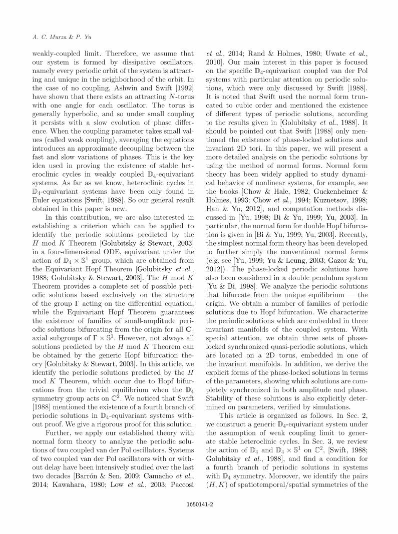
In this section, we construct an oscillatory systemwith the D4 symmetry group, which is described bya Cayley diagram. A Cayley diagram consists of aset of nodes with arrows between them. The verticesor nodes of the graph represent the group elementsand the arrows show how the generators act on theelements of the group. Let J ⊂ D4 be the generatingset of D4. This implies that

(a) J generates D4,

(b) J is finite and

(c) J = J−1.

(1)

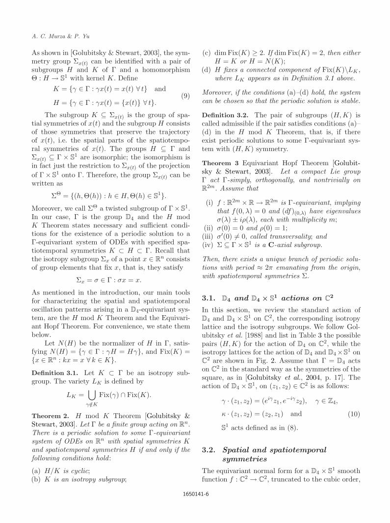
Since D4 is finite, the assumptions (b) and (c) areautomatically satisfied. The Cayley graph of D4,as shown in Fig. 1, is a directed colored graphwhose arrows indicate the action on the group ele-ments and the vertices denote the group elements.As shown in [Ashwin & Stork, 1994] the generatingset J is a set of “colors” of the directed edges, andthe group elements κi and ζj are connected throughan edge from κi to ζj of color c ∈ J if and only ifκi = ζj.

1

2

3

4

5

6

7

8

Fig. 1. A Cayley graph of the D4 group showing two gen-erators: The solid arrows representing the left-multiplicationwith κ and the dotted arrows the left-multiplication with ζ.

2.1. Eight oscillators with weakcoupling

Following the work of Ashwin and Stork [1994], wemay identify the vertices as cells with a certaindynamics and the edges as couplings between thecells. Consequently, we can construct an ODE sys-tem which has the D4 symmetry, with two genera-tors ζ and κ having act as:

ζ := (1 2 3 4)(5 6 7 8),

κ := (1 5)(2 8)(3 7)(4 6).(2)

If we assign coupling between the cells relatedby the permutations in (2), we can build the follow-ing pairwise system in R8 with the D4 symmetry,

x1 = f(x1) + g(x4, x1) + h(x5, x1),

x2 = f(x2) + g(x1, x2) + h(x8, x2),

x3 = f(x3) + g(x2, x3) + h(x7, x3),

x4 = f(x4) + g(x3, x4) + h(x6, x4),

x5 = f(x5) + g(x8, x5) + h(x6, x1),

x6 = f(x6) + g(x7, x8) + h(x2, x5),

x7 = f(x7) + g(x6, x7) + h(x3, x8),

x8 = f(x8) + g(x5, x6) + h(x4, x7)

(3)

where the dot denotes differentiation with respectto time t, f : R → R and g, h : R2 → R. Using theidea of Ashwin and Stork [1994] we may think off, g and h as being generic functions assuring thatthe isotropy of the vector field under the action ofO8 is generically D4. In the case of weak coupling,system (3) can be rewritten as an ODE system inthe form of

xi = f(xi) + εgi(x1, . . . , x8), i = 1, 2, . . . , 8, (4)

where xi ∈ R and g commutes with the permuta-tion action of D4 on R8, both f and gi are of theclass C∞. The constant ε represents the weak cou-pling. Similar to [Ashwin & Swift, 1992] or [Ash-win & Stork, 1994] we assume that each state ofsystem (4) has a hyperbolic stable limit cycle.

It has been shown in [Ashwin & Swift, 1992]that in the case of weak coupling, one should notjust consider irreducible representations of D4. Inour case, there are eight stable hyperbolic limitcycles at ε = 0, implying that the asymptoticdynamics of system (4) is decomposed into theasymptotic dynamics of eight limit cycles. This way,

1650141-3

August 1, 2016 10:10 WSPC/S0218-1274 1650141

A. C. Murza & P. Yu

we can embed the flow on an eight-dimensionaltorus T8. Again, we assume the hyperbolicity oneach of the eight limit cycles for small enough valuesof ε, which justifies the expression of the dynam-ics of the system as an ODE system in terms ofeight phases, i.e. an ODE system on T8 which is D4-equivariant. There are certain similarities betweenthe D4 and Q4 groups acting on C2 as discussedin [Ashwin et al., 1994], but they are not isomor-phic. When the coupling parameter ε is small, it ispossible to average the equations and introduce anapproximate decoupling between the fast and slowvariations of phases. This can be seen as introduc-ing phase shift symmetry which acts on T8 by atranslation along the diagonal; Rψ(φ1, . . . , φ8) :=(φ1 + ψ, . . . , φ8 + ψ), for ψ ∈ S1. We are particu-larly interested in the three-dimensional fixed-pointspaces as shown in Table 1, which are invariantunder Z2 or Z2 action. Proving the existence ofheteroclinic cycles in these two fixed-point spacesis the same, so in the following we will onlyconsider Z2.

2.2. Analysis of a family of vectorfields in Fix(Z2)

For convenience, we define the coordinates inFix(Z2) by using the following basis,

e1 =12(1, 1, 1, 1,−1,−1,−1,−1),

e2 =12(1,−1, 1,−1,−1, 1,−1, 1),

e3 =12(1,−1, 1,−1, 1,−1, 1, 1)

(5)

and consider the space spanned by {e1, e2, e3},parameterized by {ψ1, ψ2, ψ3} :

∑3n=1 ψnen. With

these coordinates, we construct the following fam-ily of three-dimensional differential systems whichsatisfy the symmetry of Fix(Z2).

ψ1 = sin(ψ1) cos(ψ2) + ε sin(4ψ1) cos(4ψ2),

ψ2 = sin(ψ2) cos(ψ3) + ε sin(4ψ2) cos(4ψ3),

Table 1. Isotropy subgroups and fixed points for the D4 × S1 action on T8.

Σ Fix(Σ) Generators dimFix(Σ)

D4 (0, 0, 0, 0, 0, 0, 0, 0, 0) (ζ, 0), (κ, 0) 0

fDa4 (0, 0, 0, 0, π, π, π, π) (ζ, π), (κ, π) 0

fDb4 (0, π, 0, π, 0, π, 0, π) (κζ, π), (κ, π) 0

fDc4 (0, π, 0, π, π, 0, π, 0) (κζ, π), (ζ2, π) 0

Z04 (0, 0, 0, 0, φ, φ, φ, φ) (ζ, 0) 1

fZπ4 (0, π, 0, π, φ, φ+ π, φ, φ+ π) (ζ, π) 1

˜Z

π/24

„0,

3π

2, π,

π

2, φ, φ+

π

2, φ+ π, φ+

3π

2

« “ζ,π

2

”1

fDa2 (0, φ, 0, φ, φ, 0, φ, 0) (κ, 0), ((0, 0), (π, π)) 1

fDb2 (0, φ, 0, φ, φ+ π, π, φ+ π, π) (κ, π), ((0, 0), (π, π)) 1

fDc2

„0, φ, π, φ+ π, φ+

3π

2,3π

2, φ+

π

2,π

2

« “κ,π

2

”, ((0, 0), (π, π)) 1

fDd2 (0, φ, 0, φ, 0, φ, 0, φ) (ζ2, 0), ((0, 0), (π, π)) 1

fDe2 (0, φ, 0, φ, π, φ+ π, π, φ+ π) (ζ2, π), ((0, 0), (π, π)) 1

fDf

2

„0, φ, π, φ+ π,

π

2, φ+

π

2,3π

2, φ+

3π

2

« “ζ2,

π

2

”, ((0, 0), (π, π)) 1

Z2 (0, φ1, 0, φ1, φ2, φ3, φ2, φ3) κ 3

fZ2 (0, φ1, π, φ1 + π,φ2, φ3, φ2 + π, φ3 + π) ζ2 3

1650141-4

August 1, 2016 10:10 WSPC/S0218-1274 1650141

Coupled Oscillatory Systems with D4 Symmetry

ψ3 = sin(ψ3) cos(ψ1) + ε sin(4ψ3) cos(4ψ1)

+ q(1 + cos(ψ1 − ψ2)) sin(4ψ3).(6)

Since the planes ψi = 0 (mod π), i = 1, 2, 3,are invariant under the flow of (6), it is clear that(π, 0, 0), (0, π, 0) and (0, 0, π) are equilibria of (6).To check the existence of heteroclinic cycles in sys-tem (6), we first linearize the system at the equilib-ria (i.e. the zero-dimensional fixed points). Withoutloss of generality, we assume that Fix(Z2) is attract-ing and therefore the stability. We analyze thedynamics within the fixed point space Fix(Z2). Inparticular, we will prove that the eigenvalues of thelinearization in each case are of opposite signs (seeTable 2), indicating the existence of such a hete-roclinic cycle between them. We use the criteria ofKrupa and Melbourne [1995] to study the stabilityof the heteroclinic cycle.

We have the following theorem.

Theorem 1. There exists a heteroclinic cycle insystem (6) in the following way :

· · ·fZπ4−→ Da

4

gZ

π/24−−−→ Db

4

fZ

04−→ Dc

4

fZπ4−→ · · · .

The heteroclinic cycle is

(A) asymptotically stable if −14 < ε < 0 and q <

18 + ε

2 ;(B) or unstable but essentially asymptotically stable

if −14 < ε < 0 and 1

8 + ε2 < q < 1

2 − (1+4ε)3

8(−1+4ε)2;

(C) or unstable if 14 > ε > 0.

Proof. In Fix(Z2) and Fix(Z2) there are no extrafixed points if |ε| < 1

4 and |ε+2q| < 14 . The stability

is given by ρ =∏3i=1 ρi, where ρi = min{ci/ei, 1 −

ti/ei}, ei is the expanding eigenvector at the ithpoint of the cycle, −ci is the contracting eigenvector

Table 2. Eigenvalues of the flow of Eq. (6) at the four non-conjugate zero-dimensional fixed points.

Fix(Σ) (ψ1, ψ2, ψ3) λ1 λ2 λ3

D4 (0, 0, 0) 1 + 4ε 1 + 4ε 1 + 4(ε+ 2q)fDa4 (π, 0, 0) −1 + 4ε −1 + 4ε 1 + 4εfDb4 (0, π, 0) −1 + 4ε −1 + 4ε 1 + 4εfDc4 (0, 0, π) −1 + 4ε 1 + 4ε −1 + 4(ε+ 2q)

and ti is the tangential eigenvector of the lineariza-tion. For the heteroclinic cycle we have

ρ1 = ρ2 =−1 + 4ε1 + 4ε

,

ρ3 =

1 − 4ε1 + 4ε

if q <18

+ε

2,

2 − 8q1 + 4ε

if q >18

+ε

2.

Then the proof follows by applying Theorem 2.4 in[Krupa & Melbourne, 1995]. �

Remark 2.1. For any 14 < ε < 0, we have 1

8 + ε2 < q <

12− (1+4ε)3

8(−1+4ε)2, and therefore there exist values of q to

yield essentially asymptotic stable heteroclinic con-nections. In consequence, there exists an attractingheteroclinic cycle even though the linear stability ofFix(Dc

2) has an expanding transverse eigenvalue.

3. The H mod K Theorem versusthe Equivariant Hopf Theorem

Consider the system

x = f(x, λ), (7)

where x ∈ C2, λ ∈ R is the bifurcation parame-ter, and f : C2 × R → C2 is smooth and commuteswith D4:

f(σ · x, λ) = σ · f(x, λ), σ ∈ D4.

We assume that at the Hopf bifurcation point(df)(0,0) has eigenvalues ±i. Since Fix(D4) = {0},it follows that f(0, λ) ≡ 0. As in [Dias & Paiva,2010], our goal is to study the generic existence ofperiodic solutions of (7) near the bifurcation point(x, λ) = (0, 0). In addition, we assume that f is inBirkhoff normal form, i.e. it commutes with S1, thuswe may assume that S1 acts on C2 by

θ · (z1, z2) = (eiθz1, eiθz2), θ ∈ S1. (8)

We call (γ, θ) ∈ Γ×S1 a spatiotemporal symme-try of the solution x(t). A spatiotemporal symmetryof x(t) for which θ = 0 is called a spatial symmetry,since it fixes the point x(t) for any t > 0. The groupof all spatiotemporal symmetries of x(t) is denotedby

Σx(t) ⊆ Γ × S1.

1650141-5

August 1, 2016 10:10 WSPC/S0218-1274 1650141

A. C. Murza & P. Yu

As shown in [Golubitsky & Stewart, 2003], the sym-metry group Σx(t) can be identified with a pair ofsubgroups H and K of Γ and a homomorphismΘ : H → S1 with kernel K. Define

K = {γ ∈ Γ : γx(t) = x(t) ∀ t} and

H = {γ ∈ Γ : γx(t) = {x(t)} ∀ t}.(9)

The subgroup K ⊆ Σx(t) is the group of spa-tial symmetries of x(t) and the subgroupH consistsof those symmetries that preserve the trajectoryof x(t), i.e. the spatial parts of the spatiotempo-ral symmetries of x(t). The groups H ⊆ Γ andΣx(t) ⊆ Γ × S1 are isomorphic; the isomorphism isin fact just the restriction to Σx(t) of the projectionof Γ× S1 onto Γ. Therefore, the group Σx(t) can bewritten as

ΣΘ = {(h,Θ(h)) : h ∈ H,Θ(h) ∈ S1}.Moreover, we call ΣΘ a twisted subgroup of Γ× S1.In our case, Γ is the group D4 and the H modK Theorem states necessary and sufficient condi-tions for the existence of a periodic solution to aΓ-equivariant system of ODEs with specified spa-tiotemporal symmetries K ⊂ H ⊂ Γ. Recall thatthe isotropy subgroup Σx of a point x ∈ Rn consistsof group elements that fix x, that is, they satisfy

Σx = σ ∈ Γ : σx = x.

As mentioned in the introduction, our main toolsfor characterizing the spatial and spatiotemporaloscillation patterns arising in a D4-equivariant sys-tem, are the H mod K Theorem and the Equivari-ant Hopf Theorem. For convenience, we state thembelow.

Let N(H) be the normalizer of H in Γ, satis-fying N(H) = {γ ∈ Γ : γH = Hγ}, and Fix(K) ={x ∈ Rn : kx = x ∀ k ∈ K}.Definition 3.1. Let K ⊂ Γ be an isotropy sub-group. The variety LK is defined by

LK =⋃γ /∈K

Fix(γ) ∩ Fix(K).

Theorem 2. H mod K Theorem [Golubitsky &Stewart, 2003]. Let Γ be a finite group acting on Rn.There is a periodic solution to some Γ-equivariantsystem of ODEs on Rn with spatial symmetries Kand spatiotemporal symmetries H if and only if thefollowing conditions hold :

(a) H/K is cyclic;(b) K is an isotropy subgroup;

(c) dim Fix(K) ≥ 2. If dim Fix(K) = 2, then eitherH = K or H = N(K);

(d) H fixes a connected component of Fix(K)\LK ,where LK appears as in Definition 3.1 above.

Moreover, if the conditions (a)–(d) hold, the systemcan be chosen so that the periodic solution is stable.

Definition 3.2. The pair of subgroups (H,K) iscalled admissible if the pair satisfies conditions (a)–(d) in the H mod K Theorem, that is, if thereexist periodic solutions to some Γ-equivariant sys-tem with (H,K) symmetry.

Theorem 3 Equivariant Hopf Theorem [Golubit-sky & Stewart, 2003]. Let a compact Lie groupΓ act Γ-simply, orthogonally, and nontrivially onR2m. Assume that

(i) f : R2m × R → R2m is Γ-equivariant, implyingthat f(0, λ) = 0 and (df)(0,λ) have eigenvaluesσ(λ) ± iρ(λ), each with multiplicity m;

(ii) σ(0) = 0 and ρ(0) = 1;(iii) σ′(0) = 0, called transversality; and(iv) Σ ⊆ Γ × S1 is a C-axial subgroup.

Then, there exists a unique branch of periodic solu-tions with period ≈ 2π emanating from the origin,with spatiotemporal symmetries Σ.

3.1. D4 and D4 × S1 actions on C2

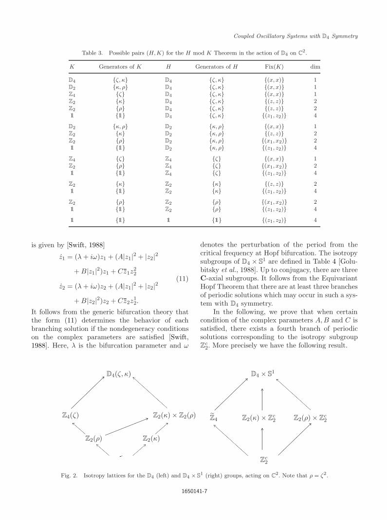
In this section, we review the standard action ofD4 and D4 × S1 on C2, the corresponding isotropylattice and the isotropy subgroups. We follow Gol-ubitsky et al. [1988] and list in Table 3 the possiblepairs (H,K) for the action of D4 on C2, while theisotropy lattices for the action of D4 and D4×S1 onC2 are shown in Fig. 2. Assume that Γ = D4 actson C2 in the standard way as the symmetries of thesquare, as in [Golubitsky et al., 2004, p. 17]. Theaction of D4 × S1, on (z1, z2) ∈ C2 is as follows:

γ · (z1, z2) = (eiγz1, e−iγz2), γ ∈ Z4,

κ · (z1, z2) = (z2, z1) and

S1 acts defined as in (8).

(10)

3.2. Spatial and spatiotemporalsymmetries

The equivariant normal form for a D4 × S1 smoothfunction f : C2 → C2, truncated to the cubic order,

1650141-6

August 1, 2016 10:10 WSPC/S0218-1274 1650141

Coupled Oscillatory Systems with D4 Symmetry

Table 3. Possible pairs (H,K) for the H mod K Theorem in the action of D4 on C2.

K Generators of K H Generators of H Fix(K) dim

D4 {ζ, κ} D4 {ζ, κ} {(x, x)} 1D2 {κ, ρ} D4 {ζ, κ} {(x, x)} 1Z4 {ζ} D4 {ζ, κ} {(x, x)} 1Z2 {κ} D4 {ζ, κ} {(z, z)} 2Z2 {ρ} D4 {ζ, κ} {(z, z)} 21 {1} D4 {ζ, κ} {(z1, z2)} 4

D2 {κ, ρ} D2 {κ, ρ} {(x, x)} 1Z2 {κ} D2 {κ, ρ} {(z, z)} 2Z2 {ρ} D2 {κ, ρ} {(x1, x2)} 21 {1} D2 {κ, ρ} {(z1, z2)} 4

Z4 {ζ} Z4 {ζ} {(x, x)} 1Z2 {ρ} Z4 {ζ} {(x1, x2)} 21 {1} Z4 {ζ} {(z1, z2)} 4

Z2 {κ} Z2 {κ} {(z, z)} 21 {1} Z2 {κ} {(z1, z2)} 4

Z2 {ρ} Z2 {ρ} {(x1, x2)} 21 {1} Z2 {ρ} {(z1, z2)} 4

1 {1} 1 {1} {(z1, z2)} 4

is given by [Swift, 1988]

z1 = (λ+ iω)z1 + (A|z1|2 + |z2|2

+B|z1|2)z1 + Cz1z22

z2 = (λ+ iω)z2 + (A|z1|2 + |z2|2

+B|z2|2)z2 + Cz2z12.

(11)

It follows from the generic bifurcation theory thatthe form (11) determines the behavior of eachbranching solution if the nondegeneracy conditionson the complex parameters are satisfied [Swift,1988]. Here, λ is the bifurcation parameter and ω

denotes the perturbation of the period from thecritical frequency at Hopf bifurcation. The isotropysubgroups of D4 × S1 are defined in Table 4 [Golu-bitsky et al., 1988]. Up to conjugacy, there are threeC-axial subgroups. It follows from the EquivariantHopf Theorem that there are at least three branchesof periodic solutions which may occur in such a sys-tem with D4 symmetry.

In the following, we prove that when certaincondition of the complex parameters A,B and C issatisfied, there exists a fourth branch of periodicsolutions corresponding to the isotropy subgroupZc2. More precisely we have the following result.

D4(ζ, κ)

Z2(κ)

Z4(ζ) Z2(κ) × Z2(ρ)

Z2(ρ)

D4 × S1

Z4 Z2(κ) × Zc2 Z2(ρ) × Z

c2

Zc2

Fig. 2. Isotropy lattices for the D4 (left) and D4 × S1 (right) groups, acting on C2. Note that ρ = ζ2.

1650141-7

August 1, 2016 10:10 WSPC/S0218-1274 1650141

A. C. Murza & P. Yu

Table 4. Spatial and spatiotemporal symmetries of solutions arising from the trivial equilibrium due to primary Hopf bifur-cation for the action of D4 × S1 on C2.

Isotropy Subgroup Subgroup of Spatiotemporal Spatial

Generators, n ≡ 0 Σ ⊂ Dn × S1 Symmetries H Symmetries K Fixed Point(mod 4) Generators Generators Generators Space Dimension

D4 × S1 {γ, κ, θ} {γ, κ} {(0, 0)(π, π)} {(0, 0)} 0eZ4 = {(γ,−γ) : γ ∈ Z4} {−γ, γ} {γ} {(0, 0)(π, π)} {(z1, 0)} 2

Z2(κ) × Zc2 {κ, [(0, 0)(π, π)]} {κ, [(0, 0)(π, π)]} {κ, [(0, 0)(π, π)]} {(z1, z1)} 2

Z2(ρ) × Zc2 {ρ, [(0, 0)(π, π)]} {ρ, [(0, 0)(π, π)]} {ρ, [(0, 0)(π, π)]} {(z1, e2πi/4z1)} 2

Zc2 {(0, 0)(π, π)} {(0, 0)(π, π)} {(0, 0)(π, π)} C2 4

Theorem 4. Consider the normal form (11). If|B|2 ≥ |C|2, then the system admits a branch ofperiodic solutions that bifurcate from (0, 0) with thesymmetry of Zc2.

Proof. We begin by introducing a change of coor-dinates: z1 = r1e

iφ1 , z2 = r1eiφ2 into (11) to obtain

the following equations at the equilibrium:

(λ+ iω)r1eiφ1 + (Ar21 + r22 +Br21)r1eiφ1

+Cr1r22ei(2φ2−φ1) = 0,

(λ+ iω)r1eiφ1 + (Ar21 + r22 +Br22)r2eiφ2

+Cr21r2ei(2φ1−φ2) = 0,

which in turn yield

(λ+ iω) + (Ar21 + r22 +Br21) + Cr22e2i(φ2−φ1) = 0,

(λ+ iω) + (Ar21 + r22 +Br21) + Cr21e2i(φ1−φ2) = 0.

(12)

Let φ = φ2−φ1. Then, combining the two equationsin (12) we obtain

r21(B − Ce2φi) = r22(B − Ce−2φi). (13)

It follows from (13) that

r2 =r22r21

=B − Ce2φi

B − Ce−2φi

=(B − Ce2φi)(B − Ce−2φi)

|B − Ce−2φi|2

=(B − Ce2φi)(B − Ce2φi)

|B − Ce−2φi|2 ≥ 0,

which implies that

Im((B − Ce2φi)(B −Ce2φi)) = 0 and

Re((B − Ce2φi)(B − Ce2φi)) ≥ 0.(14)

Let B = Br+ iBi and C = Cr+ iCi. Then, Eq. (14)yields

2(C2r + C2

i ) cos(2φ) = 2(BiCi +BrCr),

B2r +B2

i − 2(BiCi +BrCr) cos(2φ)

+ (C2r + C2

i )(cos(2φ)2 − sin(2φ)2) ≥ 0.

(15)

Substituting the first equation in (15) into the sec-ond, we obtain

|B|2 ≥ |C|2. (16)

Therefore, there always exist solutions to (11) inthe form of z1 = r1e

iφ1 , z2 = r1eiφ2 as long as the

condition (16) is satisfied, and they do not dependon φ1, φ2. In particular, we analyze the action of thegroup Zc2 on z1 = r1e

iφ1 , z2 = r2eiφ2 under the con-

dition (16). Recall that Zc2 = {(0, 0), (π, π)}. Thus,

(π, π) · (r1eiφ1 , r2eiφ2) = (r1ei(φ1+2π), r2e

iφ2)

= (r1eiφ1 , r2eiφ2),

(0, 0) · (r1eiφ1 , r2eiφ2) = (r1eiφ1 , r2e

iφ2).

In consequence, the solution is fixed by Zc2 for anyφ1, φ2. �

Moreover, we have the following theorem.

Theorem 5. For the representation of the group D4

on C2, the pairs of subgroups (H,K), satisfying theconditions of the H mod K Theorem, occur as spa-tiotemporal and spatial symmetries, respectively, ofperiodic solutions arising through a primary Hopfbifurcation, as shown in Table 5.

Proof. First, we discuss why the mentioned pairs(H,K) are admissible. For the case (i), the sub-group Z2(κ) of D4(ζ, κ) projects into the subgroupZ2(κ)×Zc2 of D4×S1. The conditions (a)–(d) of theH mod K Theorem (in Theorem 2) are satisfied.

1650141-8

August 1, 2016 10:10 WSPC/S0218-1274 1650141

Coupled Oscillatory Systems with D4 Symmetry

Table 5. Spatiotemporal symmetries of the solutions arisingfrom the trivial equilibrium due to primary Hopf bifurcationfor the action of D4 ×S1 on C2 with the corresponding solu-tion types.

Case H K Solution Types

(i) Z2(κ) Z2(κ) x1(t), x1(t), x2(t), x2(t)

(ii) Z2(ρ) Z2(ρ) x1(t), x2(t), x3(t), x2(t)

(iii) Z4(ζ) 1 x1(t), x1

„t+

1

4

«, x1

„t+

2

4

«,

x1

„t+

3

4

«(iv) 1 1 x1(t), x2(t), x3(t), x4(t)

Since Z2(κ) × Zc2 has two-dimensional fixed-pointsubspace (see Table 4), there are periodic solu-tions arising from a primary Hopf bifurcation withthe corresponding symmetry. A similar analysiscan be applied to the case (ii) for the subgroupZ2(ρ). The case (iii) corresponds to the projec-tion of the subgroup Z4(ζ) of D4(ζ, κ) acting onC2 into the corresponding cyclic subgroup Z4 ofD4 ×S2. Since it is C-axial, there is a periodic solu-tion arising from a Hopf bifurcation, with symme-try Z4. Finally, the Case (iv) corresponds to theprojection of the identity subgroup of D4, into theisotropy subgroup Zc2 of D4 × S1. In this case, itfollows from Theorem 4 that there are periodicsolutions arising from a primary Hopf bifurcation,with symmetry Zc2.

Next, we analyze why the remaining (H,K)pairs in Table 3 cannot correspond to periodic solu-tions from primary Hopf bifurcations. The first sixitems in Table 3 correspond to H = D4(κ, ρ),which is not an isotropy subgroup of D4 × S1. Sim-ilarly, the next four items in Table 3 correspond toH = D2(κ, ρ), which is also not an isotropy sub-group of D4 × S1. In the 13th item in Table 3,we have H = K = Z4(ζ). In this case, K can-not be K = Z4(ζ) since this isotropy subgrouphas a one-dimensional fixed-point subspace, whichdoes not satisfy hypothesis (c) of the H mod KTheorem. The 14th item in Table 3 corresponds to(H,K) = (Z4(ζ),Z2(ρ)). Since in this case K has atwo-dimensional fixed-point subspace, it has to beeither H = K or H = N(K), where N(K) is thenormalizer of K in D4. For the former, H = K isnot possible because H = Z4(ζ) = Z2(ρ); and thelatter is also not possible because N(K) = D2(κ,ρ) = Z4(ζ).

The cases (H,K) = (Z2(κ),1) and (H,K) =(Z2(ρ),1) in Table 5 are more interesting. Theiranalysis is similar and so we only study one of them,say (H,K) = (Z2(κ),1). If X(t) = (z1(t), z2(t))is a 2π-periodic solution of a D4-invariant differ-ential equation, with H = Z2(κ), K = 1, then forsome θ = 0 (mod 2π), and for all t > 0 we havez1(t + θ) = z1(t) and z2(t) = z2(t + 2θ). If one ofz1(t) and z2(t) is identically zero, then it followsfrom the isotropy subgroups of D4 × S1 in Table 5that the fixed-point subspaces of all isotropy sub-groups are zero-dimensional. The only other possi-bility is that all coordinates of X(t) are nonzero,i.e. X(t) = (z1(t), z2(t + θ)) where θ = ρ

2 , with θ-periodic function z1 and 2θ-periodic function z2(t).In this case, if X(t) bifurcates from an equilibriumin the normal form (11), then at the bifurcationpoint the eigenvalues would be ±2πi/θ and ±πi/θ,leading to 2:1 resonance. This last situation is notcompatible with the normal form (11), since the lin-earization of (11) at the origin is a (complex) mul-tiple of the identity.

For the isotropy subgroups K = 1, with four-dimensional fixed-point subspaces, we need to ver-ify condition (d) of the H mod K Theorem. Forevery γ ∈ Γ, it is clear that dim Fix(γ) is even,and thus LK is always the union of a finite num-ber of subspaces with even dimension. Hence, LKhas even codimension in Fix(K) and consequently,Fix(K)\LK is connected and condition (d) in the Hmod K Theorem is applicable to all isotropy sub-groups with four-dimensional fixed-point subspaces.

�

4. Case Study: Two Coupled vander Pol Oscillators

In this section, we apply the theory established inthe previous sections and use normal form theory toconsider the following two coupled planar van derPol oscillators,

x = −x+ (λ− x2 − αw2)x,

w = −w + (λ− w2 − αx2)w,(17)

where (x,w) are the coordinates in the plane R2.System (17) is equivariant under the D4 action, gen-erated by (x,w) �→ (−x,w) and (x,w) �→ (w, x).

The two coupled van der Pol oscillators havebeen studied for several decades (e.g. see [Rand &Holmes, 1980; Paccosi et al., 2014]), and found inreal applications [Kawahara, 1980; Camacho et al.,

1650141-9

August 1, 2016 10:10 WSPC/S0218-1274 1650141

A. C. Murza & P. Yu

2014]. Even three coupled van der Pol oscillators[Uwate et al., 2010] and four coupled van der Poloscillators [Barron & Sen, 2009] have also beenexplored

To initiate the linear analysis of this system, itis useful to introduce new variables, x = x1, x = x2,w = x3, w = x4, into system (17) to obtain

x1 = x2,

x2 = −x1 + (λ− x21 − αx2

3)x2,

x3 = x4,

x4 = −x3 + (λ− x23 − αx2

1)x4.

(18)

We observe that the unique equilibrium pointof system (18) is given by

E0 : (x1, x2, x3, x4) = (0, 0, 0, 0). (19)

The Jacobian matrix of system (18) evaluated at E0

has two pairs of complex conjugate eigenvalues:

12(λ−

√−4 + λ2) (twice) and

12(λ+

√−4 + λ2) (twice).

Therefore, at λ = 0, the four eigenvalues willcross the imaginary axis simultaneously and thelinearized system behaves as two coupled oscilla-tors. However, it can be shown that at the crit-ical point λ = 0, the origin of system (18) isactually globally asymptotically stable if α > 0.To achieve this, we construct the Lyapunov func-tion: V = 1

2 (x21 + x2

2 + x23 + x2

4), and hence alongthe trajectory of system (18) we have dV

dt |(18) =−[(x2

1 + αx23)x

22 + (x2

3 + αx21)x

24] ≤ 0. The equal

sign holds only if x1 = x3 = 0 or x2 = x4 = 0;but none of them is the solution of (18) except thetrivial equilibrium solution x1 = x2 = x3 = x4 = 0.Thus, by applying the LaSalles principle [LaSalle,1976], we conclude that the origin of system (18) isglobally asymptotically stable.

The corresponding normal form of system (18),given in polar coordinates, can be obtained as [Bi &Yu, 1999; Yu, 2003]:

r1 = r1

[12λ− 1

8r21 −

18α(2 − cos 2φ)r2

2 + · · ·],

r2 = r2

[12λ− 1

8r22 −

18α(2 − cos 2φ)r2

1 + · · ·],

θ1 = 1 − 18αr22 sin 2φ− 11

256r41

− α

128[3(4 − α) − 2(1 − 2α) cos 2φ]r21r

22

− α

256(9α + 2cos 2φ)r4

2 + · · · ,

θ2 = 1 +18αr21 sin 2φ− 11

256r42

− α

128[3(4 − α) − 2(1 − 2α) cos 2φ]r21r

22

− α

256(9α + 2cos 2φ)r4

1 + · · · ,(20)

where φ = θ1 − θ2, and · · · represents higher-orderterms.

4.1. Periodic and phase-lockedperiodic solutions

Consider the normalized system (18). First, it iseasy to see that there are three invariant manifolds,described by

M1 : {(x1, x2, x3, x4) ∈ R4 |x3 = x4 = 0},M2 : {(x1, x2, x3, x4) ∈ R4 |x1 = x2 = 0},M3 : {(x1, x2, x3, x4) ∈ R4 |x1 = x3, x2 = x4}.

(21)

Next, it is clear that the trivial equilibrium of (18),E0, is asymptotically stable (unstable) for λ < 0(λ > 0).

To find possible periodic solutions bifurcatingfrom E0, we use the normal form (20). Lettingr2 = 0 and ignoring the phase equation of θ2, weobtain a family of periodic solutions due to a Hopfbifurcation, given by

P1 : (x1, x2, x3, x4) = (r cos θ, r sin θ, 0, 0), (22)

where r and θ are described by the following normalform equations:

r =18r(4λ− r2 + · · ·), θ = 1 − 11

256r4 + · · · .

(23)

The periodic solution P1 is embedded in the invari-ant manifold M1. It can be seen from (23) that theHopf bifurcation is supercritical and thus the bifur-cating limit cycles, which exist for λ > 0, should bestable, restricted to the invariant manifold M1. That

1650141-10

August 1, 2016 10:10 WSPC/S0218-1274 1650141

Coupled Oscillatory Systems with D4 Symmetry

is, for λ > 0, as long as the initial conditions arechosen in the form of (x1, x2, x3, x4) = (x1, x2, 0, 0),where x1 and x2 are not simultaneously takenzero, the stable periodic solution remains on M1.However, for the whole four-dimensional space,(x3, x4) = (0, 0) is unstable due to λ > 0. Therefore,if at least one of x3 and x4 is chosen nonzero in theinitial condition, the periodic solution P1 becomesunstable.

Similarly, another family of periodic solutionsdue to another Hopf bifurcation is given by

P2 : (x1, x2, x3, x4) = (0, 0, r cos θ, r sin θ), (24)

where r and θ are determined by the following nor-mal form (23). For the same reason, when λ > 0,the periodic solution P2 is stable, embedded in theinvariant manifold M2, if the initial condition ischosen in the form (x1, x2, x3, x4) = (0, 0, x3, x4),with x3 and x4 not being simultaneously zero, butbecomes unstable in the whole four-dimensionalspace when at least one of x3 and x4 is nonzeroin the initial condition.

Further, a family of quasi-periodic solutions isgiven by

Q3 : (x1, x2, x3, x4) = (r1 cos θ1, r2 sin θ1,

r2 cos θ2, r2 sin θ2), (25)

where r1, r2, θ1 and θ2 are described by (20) withr1r2 = 0.

One important set of the quasi-periodic solu-tions is the so-called phase-locked solutions, i.e.θ1 − θ2 = const and that is why it is called “phase-locked”. Therefore, combining the last two equa-tions in (20) yields the following system:

r1 =1

128r1[64λ − 16r2

1 − 16α(2 − cos 2φ)r22 + · · ·],

r2 =1

128r2[64λ − 16r2

2 − 16α(2 − cos 2φ)r21 + · · ·],

φ = − 1256

(r21 + r22){32α sin 2φ+ (r21 − r22)

× [11 − α(9α + 2cos 2φ)]} + · · · .(26)

Letting r1 = r2 = φ = 0 yields the truncated alge-braic equations (for r21 + r22 = 0):

64λ− 16r21 − 16α(2 − cos 2φ)r22 = 0,

64λ− 16r22 − 16α(2 − cos 2φ)r21 = 0,

32α sin 2φ+ (r21 − r22)

× [11 − α(9α + 2cos 2φ)] = 0.(27)

Combining the first two equations of (27)results in

16(r21 − r22)[1 + α(cos 2φ− 2)] = 0,

which in turn gives two solutions:

r1 = r2 or cos 2φ = 2 − 1α. (28)

First consider r1 = r2. For this case, the thirdequation of (27) yields sin 2φ = 0, which gives pos-sible solutions 2φ = 0, π and 2π. When 2φ = 0, 2π,cos 2φ = 1, and when 2φ = π, cos 2φ = −1. Thus,using the first equation of (27) we obtain

r1 = r2 = 2

√λ

1 + α, (λ > 0, α > −1),

for φ = 0, π (29)

and

r1 = r2 = 2

√λ

1 + 3α,

(λ > 0, α > −1

3

),

for φ =π

2. (30)

The corresponding families of phase-locked solu-tions are approximated by

(x1, x2, x3, x4)

=

2

√λ

1 + α(cosωt, sinωt, cosωt, sinωt), or

2

√λ

1 + α(cos(ωt+ π), sin(ωt+ π),

cosωt, sinωt),(31)

where ω = 1 − 1116λ

2 for α > −1; and

(x1, x2, x3, x4) = 2

√λ

1 + 3α

(cos

(ωt+

π

2

),

sin(ωt+

π

2

), cosωt, sinωt

),

(32)

where ω = 1 − (11+26α−5α2)λ2

16(1+3α)2for α > −1

3 .Note in (31) that the first solution with φ = 0

is called an “in-phase” periodic solution, while the

1650141-11

August 1, 2016 10:10 WSPC/S0218-1274 1650141

A. C. Murza & P. Yu

second solution with φ = π is called “out-phase”periodic solution. All the three phase-locked peri-odic solutions given in (31) and (32) are located ona 2D torus which is embedded in the invariant man-ifold M3. All of these solutions imply that the twooscillators are synchronized. But only for the in-phase solution, the two oscillators are completelysynchronized with both amplitude and phase. Thesecond solution in (31) with φ = π and the solutionin (32) with φ = π

2 are only synchronized in ampli-tude. However, these two synchronized motions arenot distinctive in the phase space as shown in Figs. 5and 7.

It should also be pointed out that when α = 0,the first two equations of (18) are decoupled fromthe last two equations of (18), which may yield theperiodic solution P1 or P2, or the phase-locked solu-tions given in (31) and (32).

Next, consider cos 2φ = 2 − 1α , for which the

first equation of (27) yields

r21 + r22 = 4λ⇒ r22 = 4λ− r21. (33)

Substituting the above solution for r22 and (28) forcos 2φ into the third equation of (27) and solvingfor sin 2φ we obtain

sin 2φ =−116α

(r21 − 2λ)(1 − α)(9α + 13). (34)

Then, the identity sin22φ + cos22φ = 1 yields thefollowing equation:

1256α2

(1 − α)[(1 − α)(13 + 9α)2r41

− 4λ(1 − α)(13 + 9α)2r21

+ 4λ2(1 − α)(13 + 9α)2 + 256(1 − 3α)]

= 0. (35)

First note that α = 1 satisfies (35), for whichcos 2φ = 1 and sin 2φ = 0, which indicates that thisphase-locked solution is either in-phase (φ = 0) orout-phase (φ = π). Thus, the phase-locked solutionsare given by (for α = 1)

(x1, x2, x3, x4)

=

(r1 cosωt, r1 sinωt, r2 cosωt, r2 sinωt), or

(r1 cos(ωt+ π), r1 sin(ωt+ π),

r2 cosωt, r2 sinωt),(36)

where ω = 1 − 1116λ

2, r21 + r22 = 4λ. Note that theparticular solution of (36) for r1 = r2 is includedin (31).

Now, consider α = 1. The phase-locked solu-tions can be solved from the second factor in thesquare bracket of (35), which is a quadratic poly-nomial in r21. The discriminant of the polynomialis ∆ = −1024(3α − 1)(α − 1)(13 + 9α)2, which isrequired to be non-negative in order to get real solu-tions from the polynomial, yielding 1

3 ≤ α < 1,which guarantees that the quadratic polynomial haspositive solutions:

(r±1 , r∓2 ) = (

√2(λ± λ∗),

√2(λ∓ λ∗)), where

λ∗ =8

13 + 9α

√3α− 11 − α

. (37)

For α = 13 , r1 = r2 =

√2λ for which sin 2φ = 0,

cos 2φ = −1 yielding φ = π2 , and so the phase-

locked solution is given by

(x1, x2, x3, x4) =√

2λ(cos

(ωt+

π

2

),

sin(ωt+

π

2

), cosωt, sinωt

),

(38)

where ω = 1 − 43144λ

2. However, it is easy to seethat the above solution is actually included in thesolution given in (32).

Finally, for 13 < α < 1, the positivity of r1 and

r2 requires λ > λ∗. For this case, we have two setsof phase-locked solutions:

(x1, x2, x3, x4) = (r±1 cos(ωt± φ), r±1 sin(ωt± φ),

r∓2 cosωt, r∓2 sinωt), (39)

where

ω = − 164(13 + 9α)2

[(19α2 + 12α+ 13)

× (13 + 9α)2λ2 − 512(α + 5)(3α + 5)], (40)

φ =12

tan−1

[√(1 − α)(3α − 1)

1 − 2α

].

Summarizing the above results we have the fol-lowing theorem.

Theorem 6. For system (18), the periodic solu-tions are given by (22)–(24); and the phase-lockedperiodic solutions are given by (29)–(32) for equalamplitudes in the two oscillators, and the secondequation in (28), (33), (34), (36)–(40) for differ-ent amplitudes in the two oscillators.

1650141-12

August 1, 2016 10:10 WSPC/S0218-1274 1650141

Coupled Oscillatory Systems with D4 Symmetry

4.2. Stability analysis

It has been shown that the trivial equilibrium E0 is stable (unstable) for λ < 0 (λ > 0), and that theperiodic solutions P1 and P2 are stable for λ > 0, if restricted to the invariant manifolds M1 and M2,respectively.

In order to find stability of the phase-locked solutions, we use the Jacobian matrix of (26), given by

J(r1, r2, φ) =

λ

2− 3r21

8− 1

8αr22(2 − cos 2φ) −1

4αr1r2(2 − cos 2φ) −1

4αr1r

22 sin 2φ

−14αr1r2(2 − cos 2φ)

λ

2− 3r22

8− 1

8αr21(2 − cos 2φ) −1

4αr21r2 sin 2φ

−C1r1 − C2 −C1r2 + C2 C3

, (41)

where

C1 =1

128[32α sin 2φ+ (r21 − r22)

× (11 − 9α2 − 2α cos 2φ)],

C2 =1

128(r21 + r22)(11 − 9α2 − 2α cos 2φ),

C3 = − α

64(r21 + r22)[16 cos 2φ+ (r21 − r22) sin 2φ].

First, consider solution (31). Evaluating theJacobian J on solution (29) we obtain the charac-teristic polynomial,

P1(ξ) = (ξ + λ)(ξ +

2λα1 + α

)(ξ +

λ(1 − α)1 + α

),

which shows that the phase-locked solution (31) isstable for −1 < α < 1, and whether the solutionis in-phase or out-phase, depending upon the initialconditions, as illustrated in the simulations.

Next, consider solution (32). Similarly, evaluat-ing the Jacobian on solution (30) yields the charac-teristic polynomial,

P2(ξ) = (ξ + λ)(ξ +

λ(1 − 3α)1 + 3α

)(ξ − 2λα

1 + 3α

).

Thus, for −13 < α < 0, the phase-locked solu-

tion (32) with phase difference π2 is stable.

For α = 1, it is easy to get the characteristicpolynomial P3(ξ) = ξ (ξ + λ)2, which is a criticalcase. For α = 1

3 , we obtain the characteristic poly-nomial P4(ξ) = ξ(ξ + λ)(ξ − λ

3 ), showing that thephase-locked solution is unstable for α = 1

3 .Finally, for 1

3 < α < 1, evaluating the Jaco-bian on the phase-locked solution (39), we obtain

the characteristic polynomial,

P5(ξ) = ξ3 +2λ(9α + 1)(α + 1)

9α+ 13ξ2

+λ2(18α2 + 11α − 11)

9α+ 13ξ

− 12λ(3α− 1)(1 − α)(λ2 − λ∗2).

Since the existence of this solution requires λ > λ∗,this implies that P5(ξ) is an unstable polynomial.Hence, the phase-locked solution (39) is unstablewhen it exists for 1

3 < α < 1.We summarize the above results to obtain the

following result.

Theorem 7. For system (18), the periodic solu-tions P1 and P2 given in (22)–(24) are stable forλ > 0, if restricted to the invariant manifoldsM1 and M2, respectively. The phase-locked periodicsolutions given by (29) and (31) with phase differ-ence either 0 or π are stable for α ∈ (−1, 1), whilethat given by (30) and (32) with phase difference π

2

is stable for α ∈ (−13 , 0).

5. Simulations

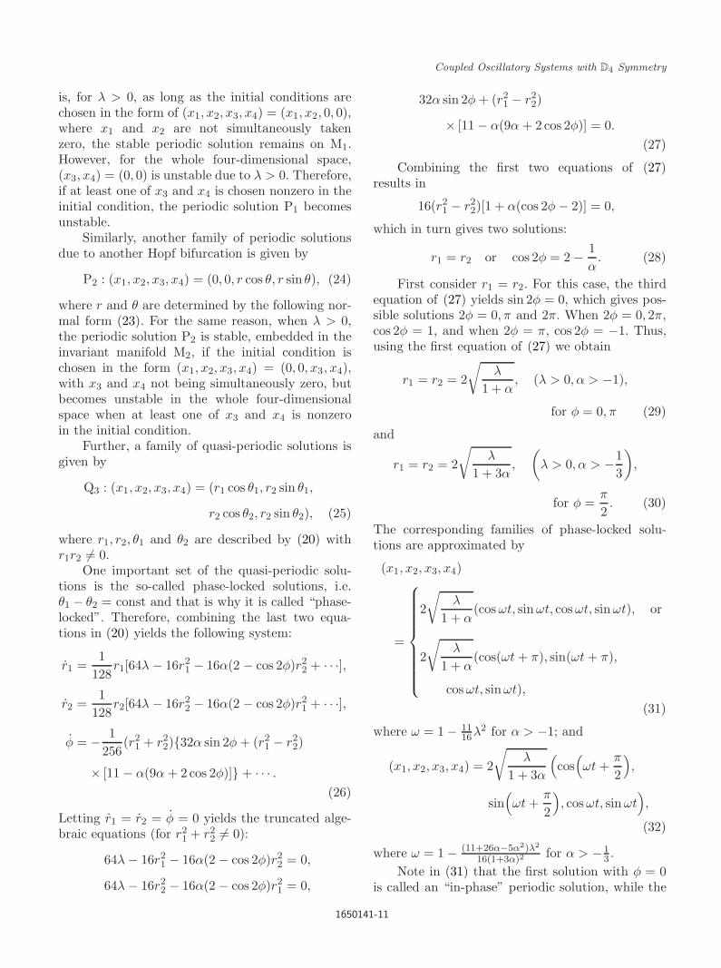
In this section, we present simulations to verify theresults we obtained in the previous section. First,we depict the cases for λ ≤ 0 with α = 1, and twovalues for λ : λ = −1 and λ = 0. The simulationsare given in Fig. 3, showing the convergence to theorigin for both cases.

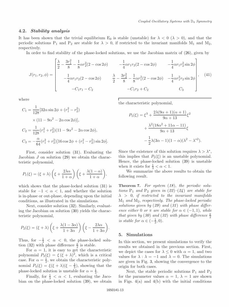
Next, the stable periodic solutions P1 and P2

for the parameter values α = 1, λ = 1 are shownin Figs. 4(a) and 4(b) with the initial conditions

1650141-13

August 1, 2016 10:10 WSPC/S0218-1274 1650141

A. C. Murza & P. Yu

0

0.5

1

1.5

2

2.5

0 10 20 30t

-2.5

-2

-1.5

-1

-0.5

x1

x4

x2

x3

-2

-1

0

1

2

-2 -1 0 1 2

x2,

x4

x1, x3

(a) (b)

Fig. 3. Simulated trajectories of system (18) for α = 1 with the initial condition (x1, x2, x3, x4) = (2, 1.5,−2,−2), convergingto the origin when (a) λ = −1 and (b) λ = 0.

(x1, x2, x3, x4) = (2,−1.5, 0, 0) and (x1, x2, x3, x4) =(0, 0, 2,−1.5), respectively.

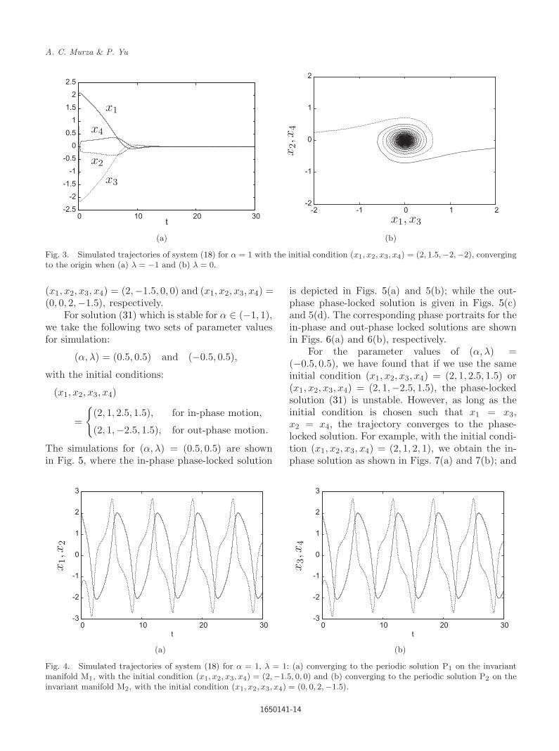
For solution (31) which is stable for α ∈ (−1, 1),we take the following two sets of parameter valuesfor simulation:

(α, λ) = (0.5, 0.5) and (−0.5, 0.5),

with the initial conditions:

(x1, x2, x3, x4)

=

{(2, 1, 2.5, 1.5), for in-phase motion,

(2, 1,−2.5, 1.5), for out-phase motion.

The simulations for (α, λ) = (0.5, 0.5) are shownin Fig. 5, where the in-phase phase-locked solution

is depicted in Figs. 5(a) and 5(b); while the out-phase phase-locked solution is given in Figs. 5(c)and 5(d). The corresponding phase portraits for thein-phase and out-phase locked solutions are shownin Figs. 6(a) and 6(b), respectively.

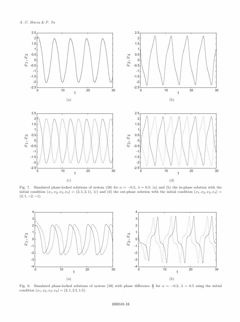
For the parameter values of (α, λ) =(−0.5, 0.5), we have found that if we use the sameinitial condition (x1, x2, x3, x4) = (2, 1, 2.5, 1.5) or(x1, x2, x3, x4) = (2, 1,−2.5, 1.5), the phase-lockedsolution (31) is unstable. However, as long as theinitial condition is chosen such that x1 = x3,x2 = x4, the trajectory converges to the phase-locked solution. For example, with the initial condi-tion (x1, x2, x3, x4) = (2, 1, 2, 1), we obtain the in-phase solution as shown in Figs. 7(a) and 7(b); and

0

1

2

3

0 10 20 30t

-3

-2

-1

x1,

x2

0

1

2

3

0 10 20 30t

-3

-2

-1

x3,

x4

(a) (b)

Fig. 4. Simulated trajectories of system (18) for α = 1, λ = 1: (a) converging to the periodic solution P1 on the invariantmanifold M1, with the initial condition (x1, x2, x3, x4) = (2,−1.5, 0, 0) and (b) converging to the periodic solution P2 on theinvariant manifold M2, with the initial condition (x1, x2, x3, x4) = (0, 0, 2,−1.5).

1650141-14

August 1, 2016 10:10 WSPC/S0218-1274 1650141

Coupled Oscillatory Systems with D4 Symmetry

-2

-1.5

-1

-0.5

0

0.5

1

1.5

2

0 10 20 30t

x1,

x3

-2

-1.5

-1

-0.5

0

0.5

1

1.5

2

0 10 20 30t

x2,

x4

(a) (b)

-2

-1.5

-1

-0.5

0

0.5

1

1.5

2

0 10 20 30t

x1,

x3

-2

-1.5

-1

-0.5

0

0.5

1

1.5

2

0 10 20 30t

x2,

x4

(c) (d)

Fig. 5. Simulated phase-locked solutions of system (18) for α = 0.5, λ = 0.5: (a) and (b) in-phase solution with the ini-tial condition (x1, x2, x3, x4) = (2, 1, 2.5, 1.5), (c) and (d) out-phase solution with the initial condition (x1, x2, x3, x4) =(2, 1,−2.5, 1.5).

-2

-1

0

1

2

-2 -1 0 1 2

x3,

x4

x1, x2

-2

-1

0

1

2

-2 -1 0 1 2

x3,

x4

x1, x2

(a) (b)

Fig. 6. Simulated phase portraits of system (18) for α = 0.5, λ = 0.5: (a) the in-phase solution in Figs. 5(a) and 5(b) and(b) the out-phase solution in Figs. 5(c) and 5(d).

1650141-15

August 1, 2016 10:10 WSPC/S0218-1274 1650141

A. C. Murza & P. Yu

-2.5

-2

-1.5

-1

-0.5

0

0.5

1

1.5

2

2.5

0 10 20 30t

x1,

x3

-2.5

-2

-1.5

-1

-0.5

0

0.5

1

1.5

2

2.5

0 10 20 30t

x2,

x4

(a) (b)

-2.5

-2

-1.5

-1

-0.5

0

0.5

1

1.5

2

2.5

0 10 20 30t

x1,

x3

-2.5

-2

-1.5

-1

-0.5

0

0.5

1

1.5

2

2.5

0 10 20 30t

x2,

x4

(c) (d)

Fig. 7. Simulated phase-locked solutions of system (18) for α = −0.5, λ = 0.5: (a) and (b) the in-phase solution with theinitial condition (x1, x2, x3, x4) = (2, 1, 2, 1), (c) and (d) the out-phase solution with the initial condition (x1, x2, x3, x4) =(2, 1,−2,−1).

-4

-3

-2

-1

0

1

2

3

4

0 10 20 30t

x1,

x3

-4

-3

-2

-1

0

1

2

3

4

0 10 20 30t

x2,

x4

(a) (b)

Fig. 8. Simulated phase-locked solutions of system (18) with phase difference π2 for α = −0.2, λ = 0.5 using the initial

condition (x1, x2, x3, x4) = (2, 1, 2.5, 1.5).

1650141-16

August 1, 2016 10:10 WSPC/S0218-1274 1650141

Coupled Oscillatory Systems with D4 Symmetry

-4

-2

0

2

4

-3 -2 -1 0 1 2 3

x2,

x4

x1, x3

Fig. 9. Simulated phase portrait of system (18) with phasedifference π

2 for α = −0.2, λ = 0.5, corresponding to the timehistory given in Fig. 8.

the out-phase solution as shown in Figs. 7(c)and 7(d) by using the initial condition (x1, x2,x3, x4) = (2, 1,−2,−1).

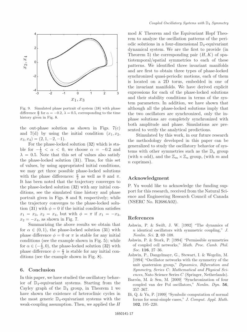
For the phase-locked solution (32) which is sta-ble for −1

3 < α < 0, we choose α = −0.2 andλ = 0.5. Note that this set of values also satisfythe phase-locked solution (31). Thus, for this setof values, by using appropriated initial conditions,we may get three possible phase-locked solutionswith the phase differences: π

2 as well as 0 and π.It has been noted that the trajectory converges tothe phase-locked solution (32) with any initial con-ditions, see the simulated time history and phaseportrait given in Figs. 8 and 9, respectively; whilethe trajectory converges to the phase-locked solu-tion (31) with φ = 0 if the initial condition satisfiesx1 = x3, x2 = x4, but with φ = π if x1 = −x3,x2 = −x4, as shown in Fig. 7.

Summarizing the above results we obtain thatfor α ∈ (0, 1), the phase-locked solution (31) withphase difference φ = 0 or π is stable for any initialconditions (see the example shown in Fig. 5); whilefor α ∈ (−1

3 , 0), the phase-locked solution (32) withphase difference φ = π

2 is stable for any initial con-ditions (see the example shown in Fig. 8).

6. Conclusion

In this paper, we have studied the oscillatory behav-ior of D4-equivariant systems. Starting from theCayley graph of the D4 group, in Theorem 1 wehave shown the existence of heteroclinic cycles inthe most generic D4-equivariant systems with theweak-coupling assumption. Then, we applied the H

mod K Theorem and the Equivariant Hopf Theo-rem to analyze the oscillation patterns of the peri-odic solutions in a four-dimensional D4-equivariantdynamical system. We are the first to provide (inTheorem 5) the corresponding pair (H,K) of spa-tiotemporal/spatial symmetries to each of thesepatterns. We identified three invariant manifoldsand are first to obtain three types of phase-lockedsynchronized quasi-periodic motions, each of themis located on a 2D torus, embedded in one ofthe invariant manifolds. We have derived explicitexpressions for each of the phase-locked solutionsand their stability conditions in terms of the sys-tem parameters. In addition, we have shown thatalthough all the phase-locked solutions imply thatthe two oscillators are synchronized, only the in-phase solutions are completely synchronized withboth amplitude and phase. Simulations are pre-sented to verify the analytical predictions.

Stimulated by this work, in our future researchthe methodology developed in this paper can begeneralized to study the oscillatory behavior of sys-tems with other symmetries such as the Dn group(with n odd), and the Zm×Zn group, (with m andn coprimes).

Acknowledgment

P. Yu would like to acknowledge the funding sup-port for this research, received from the Natural Sci-ence and Engineering Research Council of Canada(NSERC No. R2686A02).

References

Ashwin, P. & Swift, J. W. [1992] “The dynamics ofn identical oscillators with symmetric coupling,” J.Nonlin. Sci. 2, 69–108.

Ashwin, P. & Stork, P. [1994] “Permissible symmetriesof coupled cell networks,” Math. Proc. Camb. Phil.Soc. 116, 27–36.

Ashwin, P., Dangelmayr, G., Stewart, I. & Wegelin, M.[1994] “Oscillator networks with the symmetry of theunit quaternion group,” Dynamics, Bifurcation andSymmetry, Series C : Mathematical and Physical Sci-ences, Nato Science Series C (Springer, Netherlands).

Barron, M. & Sen, M. [2009] “Synchronization of fourcoupled van der Pol oscillators,” Nonlin. Dyn. 56,357–367.

Bi, Q. & Yu, P. [1999] “Symbolic computation of normalforms for semi-simple cases,” J. Comput. Appl. Math.102, 195–220.

1650141-17

August 1, 2016 10:10 WSPC/S0218-1274 1650141

A. C. Murza & P. Yu

Buono, P. L., Golubitsky, M. & Palacios, A. [2000] “Het-eroclinic cycles in rings of coupled cells,” Physica D143, 74–108.

Camacho, E., Rand, R. H. & Howland, H. [2014]“Dynamics of two van der Pol oscillators coupled viaa bath,” Int. J. Solids Struct. 41, 2133–2143.

Chow, S. N. & Hale, J. K. [1982] Methods of BifurcationTheory (Springer, NY).

Chow, S. N., Li, C. C. & Wang, D. [1994] Normal Formsand Bifurcation of Planar Vector Fields (CambridgeUniversity Press, Cambridge).

Dias, A. P. S. & Paiva, R. C. [2010] “A note on Hopfbifurcation with dihedral group symmetry,” GlasgowMath. J. 48, 41–51.

Gazor, M. & Yu, P. [2012] “Spectral sequences and para-metric normal forms,” J. Diff. Eqs. 252, 1003–1031.

Golubitsky, M., Stewart, I. & Schaeffer, D. [1988]Singularities and Groups in Bifurcation Theory II,Applied Mathematical Sciences, Vol. 69 (Springer-Verlag, NY).

Golubitsky, M. & Stewart, I. [2003] The Symmetry Per-spective: From Equilibrium to Chaos in Phase Spaceand Physical Space (Birkhauser-Verlag, Berlin).

Golubitsky, M., Shiau, L. J. & Torok, A. [2004] “Sym-metry and pattern formation on the visual cortex,”Dynamics and Bifurcation of Patterns in DissipativeSystems, World Scientific Series on Nonlinear ScienceSeries, Vol. 12 (World Scientific, Singapore).

Guckenheimer, J. & Holmes, P. [1993] NonlinearOscillations, Dynamical Systems, and Bifurcations ofVector Fields, 4th edition (Springer, NY).

Han, M. & Yu, P. [2012] Normal Forms, Mel-nikov Functions, and Bifurcations of Limit Cycles(Springer, NY).

Hou, C. & Golubitsky, M. [1997] “An example of sym-metry breaking to heteroclinic cycles,” J. Diff. Eqs.133, 30–48.

Kawahara, T. [1980] “Coupled van der Pol oscillators —A model of excitatory and inhibitory neural interac-tions,” Biol. Cybern. 39, 37–43.

Krupa, M. & Melbourne, I. [1995] “Asymptotic stabilityof heteroclinic cycles in systems with symmetry,” Erg.Th. Dyn. Syst. 15, 121–147.

Kuznetsov, Yu. A. [1998] Elements of Applied Bifurca-tion Theory, 2nd edition (Springer, NY).

LaSalle, J. P. [1976] The Stability of Dynamics Systems(SIAM, Philadelphia).

Low, L. A., Reinhall, P. G. & Storti, D. W. [2003] “Aninvestigation of coupled van der Pol oscillators,” J.Vibr. Acoust. 125, 162–169.

Paccosi, R. G., Figliola, A. & Galan-Vioque, J. [2014] “Abifurcation approach to the synchronization of cou-pled van der Pol oscillators,” SIAM J. Appl. Dyn.Syst. 13, 1152–1167.

Rand, R. H. & Holmes, P. J. [1980] “Bifurcation of peri-odic motions in two weakly coupled van der Pol oscil-lators,” Int. J. Non-Lin. Mech. 15, 387–399.

Swift, J. W. [1988] “Hopf bifurcation with the symmetryof the square,” Nonlinearity 1, 333–377.

Takamatsu, A., Tanaka, R., Yamamoto, T. & Fujii, T.[2003] “Control of oscillation patterns in a symmet-ric coupled biological oscillator system,” Proc. AIPConf., pp. 230–235.

Uwate, Y., Nishio, Y. & Stoop, R. [2010] “Synchro-nization in three coupled van der Pol oscillatorswith different coupling strength,” 2010 Int. Work-shop on Nonlinear Circuits, Communication and Sig-nal Processing, NCSP’10, Waikiki, Hawaii, March 3–5,2010.

Yu, P. [1998] “Computation of normal forms via a per-turbation technique,” J. Sound Vibr. 211, 19–38.

Yu, P. & Bi, Q. [1998] “Analysis of non-linear dynam-ics and bifurcations of a double pendulum,” J. SoundVibr. 217, 691–736.

Yu, P. [1999] “Simplest normal forms of Hopf and gen-eralized Hopf bifurcations,” Int. J. Bifurcation andChaos 9, 1917–1939.

Yu, P. [2003] “A simple and efficient method for com-puting center manifold and normal forms associatedwith semi-simple cases,” Dyn. Contin. Discr. Impuls.Syst. Ser. B : Appl. Algorith. 10, 273–286.

Yu, P. & Leung, A. Y. T. [2003] “The simplest nor-mal form of Hopf bifurcation,” Nonlinearity 16, 277–300.

1650141-18