Robert G. Parker, Yi Guo, Tugan Eritenel, and Tristan M. EricsonThe Ohio State University, Columbus, Ohio

Vibration Propagation of Gear Dynamics in aGear-Bearing-Housing System UsingMathematical Modeling and FiniteElement Analysis

NASA/CR—2012-217664

August 2012

https://ntrs.nasa.gov/search.jsp?R=20120013868 2020-04-09T12:28:25+00:00Z

NASA STI Program . . . in Profi le

Since its founding, NASA has been dedicated to the advancement of aeronautics and space science. The NASA Scientifi c and Technical Information (STI) program plays a key part in helping NASA maintain this important role.

The NASA STI Program operates under the auspices of the Agency Chief Information Offi cer. It collects, organizes, provides for archiving, and disseminates NASA’s STI. The NASA STI program provides access to the NASA Aeronautics and Space Database and its public interface, the NASA Technical Reports Server, thus providing one of the largest collections of aeronautical and space science STI in the world. Results are published in both non-NASA channels and by NASA in the NASA STI Report Series, which includes the following report types: • TECHNICAL PUBLICATION. Reports of

completed research or a major signifi cant phase of research that present the results of NASA programs and include extensive data or theoretical analysis. Includes compilations of signifi cant scientifi c and technical data and information deemed to be of continuing reference value. NASA counterpart of peer-reviewed formal professional papers but has less stringent limitations on manuscript length and extent of graphic presentations.

• TECHNICAL MEMORANDUM. Scientifi c

and technical fi ndings that are preliminary or of specialized interest, e.g., quick release reports, working papers, and bibliographies that contain minimal annotation. Does not contain extensive analysis.

• CONTRACTOR REPORT. Scientifi c and

technical fi ndings by NASA-sponsored contractors and grantees.

• CONFERENCE PUBLICATION. Collected papers from scientifi c and technical conferences, symposia, seminars, or other meetings sponsored or cosponsored by NASA.

• SPECIAL PUBLICATION. Scientifi c,

technical, or historical information from NASA programs, projects, and missions, often concerned with subjects having substantial public interest.

• TECHNICAL TRANSLATION. English-

language translations of foreign scientifi c and technical material pertinent to NASA’s mission.

Specialized services also include creating custom thesauri, building customized databases, organizing and publishing research results.

For more information about the NASA STI program, see the following:

• Access the NASA STI program home page at http://www.sti.nasa.gov

• E-mail your question to help@sti.nasa.gov • Fax your question to the NASA STI

Information Desk at 443–757–5803 • Phone the NASA STI Information Desk at 443–757–5802 • Write to:

STI Information Desk NASA Center for AeroSpace Information 7115 Standard Drive Hanover, MD 21076–1320

Robert G. Parker, Yi Guo, Tugan Eritenel, and Tristan M. EricsonThe Ohio State University, Columbus, Ohio

Vibration Propagation of Gear Dynamics in aGear-Bearing-Housing System UsingMathematical Modeling and FiniteElement Analysis

NASA/CR—2012-217664

August 2012

National Aeronautics andSpace Administration

Glenn Research CenterCleveland, Ohio 44135

Prepared under Contract NNC08CB03C

Available from

NASA Center for Aerospace Information7115 Standard DriveHanover, MD 21076–1320

National Technical Information Service5301 Shawnee Road

Alexandria, VA 22312

Available electronically at http://www.sti.nasa.gov

Trade names and trademarks are used in this report for identifi cation only. Their usage does not constitute an offi cial endorsement, either expressed or implied, by the National Aeronautics and

Space Administration.

This work was sponsored by the Fundamental Aeronautics Program at the NASA Glenn Research Center.

Level of Review: This material has been technically reviewed by NASA technical management OR expert reviewer(s).

Vibration Propagation of Gear Dynamics in a Gear-Bearing-Housing System Using

Mathematical Modeling and Finite Element Analysis

Robert G. Parker, Yi Guo, Tugan Eritenel, and Tristan M. Ericson

The Ohio State University Columbus, Ohio 43210

NASA/CR—2012-217664 1

Contents

1 Introduction 9

2 Preliminary Step: Experimental Modal Test 11

2.1 Translational Impact to Gear Tooth . . . . . . . . . . . . . . . . . . . . . . . . . 12

2.2 Translational Impact to Gear Shaft . . . . . . . . . . . . . . . . . . . . . . . . . 13

2.3 Impact to Gearbox Input Shaft . . . . . . . . . . . . . . . . . . . . . . . . . . . 14

2.4 Impact to Rear of Gearbox Housing . . . . . . . . . . . . . . . . . . . . . . . . . 15

2.5 Impact Test Summary . . . . . . . . . . . . . . . . . . . . . . . . . . . . . . . . 16

3 Gearbox Vibro-Acoustic Propagation Analysis Method Overview 17

4 Finite Element/Contact Mechanics Modeling and Analysis of the Gearbox 19

4.1 Gearbox Modeling Overview . . . . . . . . . . . . . . . . . . . . . . . . . . . . . 19

4.1.1 Contact Solver . . . . . . . . . . . . . . . . . . . . . . . . . . . . . . . . 20

4.2 Fluid Film Wave Bearing Modeling . . . . . . . . . . . . . . . . . . . . . . . . . 23

4.3 Rolling Element Bearing Modeling and Analysis . . . . . . . . . . . . . . . . . . 23

4.3.1 Cross-Coupling Bearing Stiffnesses . . . . . . . . . . . . . . . . . . . . . 25

4.4 Gear Transmission Error . . . . . . . . . . . . . . . . . . . . . . . . . . . . . . . 26

4.5 Shaft Modeling and Validation . . . . . . . . . . . . . . . . . . . . . . . . . . . . 28

4.6 Dynamic Analysis and Correlation with Experiments . . . . . . . . . . . . . . . 30

5 Analytical Gearbox Dynamic Modeling and Analysis 32

5.1 The Gear Pair . . . . . . . . . . . . . . . . . . . . . . . . . . . . . . . . . . . . . 32

5.2 Incorporating Housing Compliance with the Analytical Gear/Shaft Model . . . . 39

5.2.1 Including the Housing by Using Influence Coefficients . . . . . . . . . . . 41

5.3 Dynamic Analysis Using the Analytical Model . . . . . . . . . . . . . . . . . . . 41

6 Acoustic Radiation Gearbox Modeling and Analysis 43

6.1 Model Validation and Mesh Convergence Study . . . . . . . . . . . . . . . . . . 43

6.2 Sound Pressure and Power Computation Using Transfer Functions . . . . . . . . 45

6.3 Radiated Noise Correlation with Measurements . . . . . . . . . . . . . . . . . . 47

6.4 Noise Radiation Properties with Different Bearings . . . . . . . . . . . . . . . . 51

NASA/CR—2012-217664 2

7 Summary and Conclusions 52

NASA/CR—2012-217664 3

List of Figures

1 Fluid film wave bearing. . . . . . . . . . . . . . . . . . . . . . . . . . . . . . . . 11

2 Nine mounting locations for additional OSU accelerometers in and around gearbox. 12

3 Impact locations for relevant tests: (a) translational impact to gear tooth with

accelerometers A5 and A6 mounted to the pinion shaft, (b) impact to output gear

shaft with accelerometers A5 and A6 mounted to the pinion shaft, (c) impact to

rig input shaft with accelerometers A8 and A9 mounted to the input shaft, (d)

impact to rear of gearbox housing with accelerometers A3, A4 and A7 mounted

to the gearbox housing. . . . . . . . . . . . . . . . . . . . . . . . . . . . . . . . . 13

4 Frequency response functions for impact test to output gear tooth with accelerom-

eters A5 and A6 mounted to the pinion shaft and accelerometers A1 and A2

mounted to the input shaft pillow block for (a) mean NASA accelerometers and

(b) select OSU accelerometers. . . . . . . . . . . . . . . . . . . . . . . . . . . . . 14

5 Frequency response comparison for (a) impact to pinion gear tooth, and (b) im-

pact to gear shaft. . . . . . . . . . . . . . . . . . . . . . . . . . . . . . . . . . . 14

6 Frequency response functions for impact test to gearbox input shaft with ac-

celerometers A8 and A9 mounted to the input shaft and accelerometers A1 and

A2 mounted to the input shaft pillow block for (a) four NASA accelerometers

and (b) select OSU accelerometers. . . . . . . . . . . . . . . . . . . . . . . . . . 15

7 Frequency response functions for impact test to rear of gearbox housing with

accelerometers A3 and A4 mounted to the front and rear of gearbox respectively

and accelerometers A1 and A2 mounted to the input shaft pillow block for (a)

mean NASA accelerometers and (b) select OSU accelerometers. . . . . . . . . . 16

8 (a) Outside and (b) inside of the gearbox at NASA Glenn Research Center. . . . 18

9 Key steps to perform the gearbox acoustic analysis. . . . . . . . . . . . . . . . . 19

10 Cut-away finite element mesh of the radial ball bearing used in the gearbox (di-

mensions detailed in Table 2) and a double-row cylindrical rolling element bearing

(from a helicopter application). . . . . . . . . . . . . . . . . . . . . . . . . . . . 21

11 Assembly of the gear-bearing-shaft-housing model. . . . . . . . . . . . . . . . . . 22

12 (a) Mating gears in the NASA GRC gearbox; (b) contact pressure on gear teeth

over one mesh cycle; . . . . . . . . . . . . . . . . . . . . . . . . . . . . . . . . . 23

NASA/CR—2012-217664 4

13 (a) Finite element model of a double row cylindrical bearing (outer race is re-

moved); (b) contact pattern on one of the loaded cylinders. . . . . . . . . . . . . 24

14 Radial stiffness of examined cylindrical bearing and radial ball bearing vs. applied

radial loads calculated by the Harris (−) [1], Gargiulo (·−·−) [2], and While (−−)

[3] models. The While [3] model is modified to use ΔFΔq

to calculate the stiffness

instead of Fq. . . . . . . . . . . . . . . . . . . . . . . . . . . . . . . . . . . . . . . 25

15 Comparison between the proposed method with zero (· · ·� · · · ) and 0.01mm

(· − � · −) radial clearances and Kraus et al.’s [4] experiment (− ◦ −) for radial

and axial stiffness of the ball bearing in [4] under axial preloads. . . . . . . . . . 26

16 Comparison between the proposed method (· · ·� · · · ) and Royston and Basdogan

[5] experiment (− ◦ −) for radial and axial stiffness of self-aligning ball bearing

in [5] under radial and axial preloads, respectively. . . . . . . . . . . . . . . . . . 27

17 (a) Radial and (b) tilting stiffness of the cylindrical bearing over a ball pass

period. The bottom figures show the number of rolling elements in contact over a

ball pass period. The applied load and moment are 1000N and 1Nm, respectively. 28

18 (a) Radial and (b) tilting stiffness of the ball bearing over a ball pass period. The

bottom figures show the number of rolling elements in contact over a ball pass

period. The applied load and moment are 1000N and 1Nm, respectively. . . . . 29

19 Numerical torque impulse response of gear dynamic transmission error with fully-

populated (−) and diagonal (−−) stiffness matrices of the rolling element bearings

mounted in the examined gearbox based on [6]. The input torque equals 84.74Nm. 30

20 Coordinates of the examined gear pair. . . . . . . . . . . . . . . . . . . . . . . . 30

21 Static transmission error of the gear pair without the shaft and bearing compli-

ance. The results are calculated by finite element (−), Program X (−·−), NASA

DANST (· · · ), and Load Distribution Program (−−). The torque equals 79.09Nm. 31

22 Peak to peak amplitude of static transmission error of the gear pair with (−×−)

and without (− ◦ −) shafts at different torques. . . . . . . . . . . . . . . . . . . 32

NASA/CR—2012-217664 5

23 (a) Input shaft bending deformation calculated by analytical beam theory (solid

line) and finite element method (square marker) with simply-supported boundary

conditions under various input torques; (b) Input shaft torsional deformation cal-

culated by analytical beam theory (solid line) and finite element method (square

marker) with clamped-free boundary conditions under various input torques. The

shaft has uniform outer diameter (30.23mm). . . . . . . . . . . . . . . . . . . . 33

24 Shaft bending deformation under various input torques. . . . . . . . . . . . . . . 34

25 Numerical impulse test results of (a) dynamic transmission error and (b) the

input shaft horizontal displacement of the gear-bearing-housing system within

speed range from 0Hz to 7000Hz. The applied torque is 79.09Nm. . . . . . . . 35

26 Analytical model of the gear pair. The parameters are defined in [7]. The dashed

line is at the center of the active facewidth. . . . . . . . . . . . . . . . . . . . . . 36

27 (a) Distributed spring network over a contact line with the local and bulk stiff-

nesses, kcl(t) and kb. (b) Local kcl(t) and bulk kb stiffnesses are combined into

contact stiffness ki(q, t) by Eq. (14). . . . . . . . . . . . . . . . . . . . . . . . . . 37

28 Static transmission error from the analytical (solid line) and finite element (cir-

cles) model. (a) A helical gear pair. Quadratic tip relief starting at α = 28 deg

and root relief at α = 27 deg. Tip relief, root relief, and circular lead crown are

10 μm. The applied torque is 200 N-m. (b) Spur gear pair in [8]. Linear tip relief

starting at α = 23.6 deg with amplitude 10 μm. Circular lead crown is 5 μm.

The applied torque is 340 N-m. . . . . . . . . . . . . . . . . . . . . . . . . . . . 39

29 Description of the connection between the gears, shafts and bearings to the hous-

ing model. . . . . . . . . . . . . . . . . . . . . . . . . . . . . . . . . . . . . . . . 41

30 Graphical representation of the 12th mode at 3893 Hz (mesh deflection mode)

from the system with ball/cylindrical bearings with housing. . . . . . . . . . . . 43

31 Peak-to-peak dynamic transmission error of four systems. Analysis with roller

element bearings are marked by B, analysis with wave bearings are marked by

W, analysis including the housing flexibility is marked by H, analysis without the

housing is marked by nH. . . . . . . . . . . . . . . . . . . . . . . . . . . . . . . 44

32 Dynamic bearing forces. Analysis with roller element bearings are marked by

B, analysis with wave bearings are marked by W, analysis including the housing

flexibility is marked by H, analysis without the housing is marked by nH. . . . . 45

NASA/CR—2012-217664 6

33 Boundary element model of the gearbox established in Coustyx. . . . . . . . . . 46

34 Theoretical solutions used to validate the boundary element housing model. Noise

radiated from the housing with monopole velocity field at the gearbox surface as

the boundary condition equals to that with monopole in the free space. . . . . . 47

35 Effects of boundary element length on the relative error of calculated sound pres-

sure compared to the theoretical solution. . . . . . . . . . . . . . . . . . . . . . 48

36 Sound pressure at the NASA microphone 1 location calculated by Coustyx (�)

and theoretical models (−). . . . . . . . . . . . . . . . . . . . . . . . . . . . . . 49

37 Sound pressure transfer functions when unit dynamic loads are applied at bear-

ings. Six transfer functions are generated per each bearing along x, y, z, θx, θy, θz

directions. The input torque is 79.09Nm. . . . . . . . . . . . . . . . . . . . . . 49

38 Microphones (1 and 2) mounted above the NASA GRC gearbox. . . . . . . . . . 50

39 The time average of the experimental (−−) and calculated (−) mean squared

sound pressure at the microphone 1 location within mesh frequency range from

500 to 3000Hz. The applied torque is 79.09Nm. . . . . . . . . . . . . . . . . . 50

40 Frequency spectrum of the measured (left) and simulated (right) sound pressure

at the microphone 1 location when mesh frequency is 2000Hz. The applied

torque is 79.09Nm. . . . . . . . . . . . . . . . . . . . . . . . . . . . . . . . . . . 51

41 The frequency spectrum of the measured (left) and computed (right) sound pres-

sure at the microphone 1 location when mesh frequency is between 1000Hz and

2500Hz. The applied torque is 79.09Nm. . . . . . . . . . . . . . . . . . . . . . 52

42 Sound power of radiated gearbox noise excited by certain mesh frequency har-

monics of bearing forces with rolling element (−) and fluid film wave bearings

(−−) at 79.09Nm input torque. The excitation from 1st to 6th mesh frequency

harmonics of bearing forces are considered during the computation. A weighing

filter (ISO standard) is used to adjust sound pressure levels. . . . . . . . . . . . 53

NASA/CR—2012-217664 7

List of Tables

1 Natural frequencies observed in the NASA GRC gear test rig by impact testing. 17

2 Single row cylindrical roller and ball bearing parameters. . . . . . . . . . . . . . 20

3 Dimensions of the spur gear pair . . . . . . . . . . . . . . . . . . . . . . . . . . 21

4 Natural frequencies predicted by numerical impulse tests and measurements (Hz) 31

5 Natural frequencies of the NASA gearbox with cylindrical roller/ball bearings,

wave bearings, with housing flexibility and without housing flexibility. The mesh

deflection mode natural frequencies are highlighted. . . . . . . . . . . . . . . . . 42

NASA/CR—2012-217664 8

Abstract

Vibration and noise caused by gear dynamics at the meshing teeth propagate through

power transmission components to the surrounding environment. The purpose of this

work is to develop computational tools to investigate the vibro-acoustic propagation of

gear vibration and to investigate the effect of different bearing types on noise radia-

tion. Detailed finite element/contact mechanics and boundary element models of the

gear/bearing/housing system are established to compute the system vibration and noise

propagation. Both vibration and acoustic models are validated by experiments including

vibration modal testing and sound field measurements.

Bearings are critical components in drivetrains. Accurate modeling of rolling element

bearings is essential to assess vibration and noise of drivetrain systems. This study also

seeks to fully describe the vibro-acoustic propagation of gear dynamics through a power-

transmission system using rolling element and fluid film wave bearings. Fluid film wave

bearings have higher damping than rolling element bearings and so could offer an energy

dissipation mechanism that reduces the gearbox noise. The effectiveness of each bearing

type to disrupt vibration propagation is explored using multi-body computational models.

These models take into account gears, shafts, rolling element and fluid film wave bearings,

and the housing. Radiated noise is mapped from the gearbox surface to surrounding

environment. The effectiveness of each bearing type to disrupt vibration propagation is

speed-dependent. Housing plays an important role in noise radiation. It, however, has

limited effects on gear dynamics.

1 Introduction

Gearbox vibration contributes the structural-borne noise in helicopters [9]. The gearbox

noise consists of a wide range of gear mesh, shaft, and bearing frequencies within relative

lower audio frequency range than the jet engine noise, which is another source of helicopter

structural-borne noise. Systematic studies of the noise and vibration behavior are essential

to design quiet helicopters and to identify noise and vibration sources. Limited work has,

however, investigated the relationship between the gearbox noise and vibration.

Experimental vibro-acoustic analysis of helicopters requires effort [9, 10, 11, 12, 13]

because advanced signal processing techniques are needed to separate the gear, shaft, and

bearing signals [14]. The analytical or computational vibro-acoustic analysis of geared sys-

tems is also sparse [15] in the literature due to the complexity of these problems. Structural-

borne noise calculations of geared systems are, furthermore, semi-empirical [16, 17]. These

NASA/CR—2012-217664 9

acoustic models are not able to capture realistic dimensions of gearboxes which often

have complicated structures, which affect the noise estimate. This work defines the vibro-

acoustic behavior of gear dynamics through power-transmission systems using multi-body

dynamics gearbox models established in [18, 19] and an in-house program.

Dynamic forces at the meshing teeth drive a system vibration through power trans-

mission components to the fuselage. The bearings linking the gear shafts to the housing

are a primary factor in this noise path. Fluid film wave bearings are a special type of

journal bearings, which have waved inner diameters of the stationary bearing sides shown

in Figure 1. The wave profile amplitude is a few micrometer so that it is not obvious

in this figure. The wave bearing technology used for gas turbine lubrication [20, 21] is

recently applied to the planet bearings used in aviation planetary gears [22, 23, 20]. This

technology provides higher stiffness and better lubrication for the bearings. Experiments

on an aviation gearbox [22] with wave bearings demonstrate 25% higher load capacity com-

pared to plain journal bearings. Dimofte [20] compared the load capacity between wave

and journal bearings through an analytical formulation. He concluded that wave bearings

are more stable than plain journal bearings under light-load or unloaded conditions in any

operating regime. Furthermore, wave amplitude and starting positions of the wave profiles

are important parameters affecting wave bearing performance.

Machinery applications use rolling element bearings that do not create meaningful

damping to reduce the transmitted structural-borne noise. Wave bearings have higher

damping [24] and could offer energy dissipation. If fluid film wave bearings are shown to

withstand harsh operating conditions and provide better vibration characteristics, they

may prove an attractive alternative to standard rolling element bearings.

The major objectives of this study are to: 1) develop a finite element gearbox model

which includes the detailed contact analysis of the gear tooth mesh and individual bearing

rolling elements; 2) build up analytical (lumped parameter) model of the gear/bearing/housing

system, which provides efficient dynamic analysis; 3) establish a boundary element model

of the gearbox housing and map the radiated noise from the gearbox surface through

acoustic analysis; 4) validate the vibration and acoustic models of the examined gearbox

against measurements and theoretical solutions in the literature; and 5) understand the

effectiveness of fluid film wave bearings in breaking the vibro-acoustic propagation path

from the gears to the housing.

NASA/CR—2012-217664 10

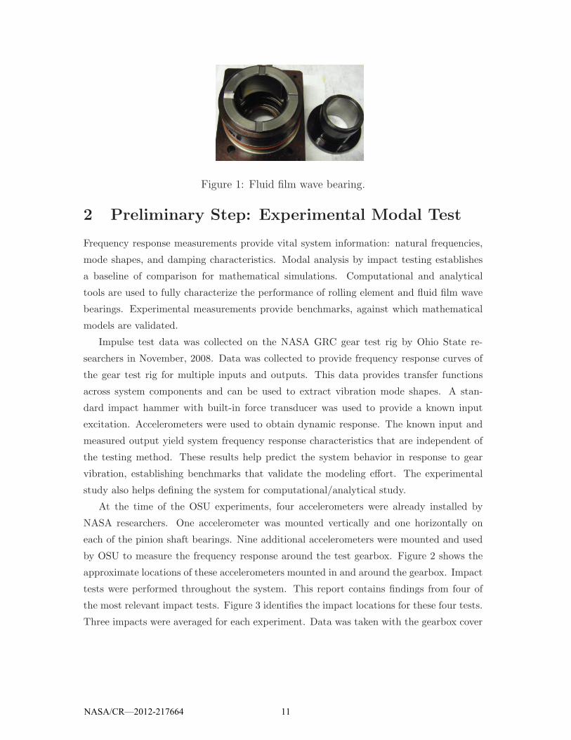
Figure 1: Fluid film wave bearing.

2 Preliminary Step: Experimental Modal Test

Frequency response measurements provide vital system information: natural frequencies,

mode shapes, and damping characteristics. Modal analysis by impact testing establishes

a baseline of comparison for mathematical simulations. Computational and analytical

tools are used to fully characterize the performance of rolling element and fluid film wave

bearings. Experimental measurements provide benchmarks, against which mathematical

models are validated.

Impulse test data was collected on the NASA GRC gear test rig by Ohio State re-

searchers in November, 2008. Data was collected to provide frequency response curves of

the gear test rig for multiple inputs and outputs. This data provides transfer functions

across system components and can be used to extract vibration mode shapes. A stan-

dard impact hammer with built-in force transducer was used to provide a known input

excitation. Accelerometers were used to obtain dynamic response. The known input and

measured output yield system frequency response characteristics that are independent of

the testing method. These results help predict the system behavior in response to gear

vibration, establishing benchmarks that validate the modeling effort. The experimental

study also helps defining the system for computational/analytical study.

At the time of the OSU experiments, four accelerometers were already installed by

NASA researchers. One accelerometer was mounted vertically and one horizontally on

each of the pinion shaft bearings. Nine additional accelerometers were mounted and used

by OSU to measure the frequency response around the test gearbox. Figure 2 shows the

approximate locations of these accelerometers mounted in and around the gearbox. Impact

tests were performed throughout the system. This report contains findings from four of

the most relevant impact tests. Figure 3 identifies the impact locations for these four tests.

Three impacts were averaged for each experiment. Data was taken with the gearbox cover

NASA/CR—2012-217664 11

off to measure vibrations inside the gearbox. The subsequent results are shown on a dB

scale.

Figure 2: Nine mounting locations for additional OSU accelerometers in and around gearbox.

2.1 Translational Impact to Gear Tooth

In this test an impact was made to a gear tooth to simulate excitation near the meshing

gears. Figure 3(a) shows the impact point and two relevant accelerometers mounted on

the pinion shaft (A5 and A6). The averaged frequency response function from the NASA

accelerometers is shown in Figure 4(a). The frequency response functions from the relevant

OSU accelerometers for this test are shown in Figure 4(b).

The data in Figure 4 shows distinct natural frequencies at 750Hz and 2500Hz in the

NASA bearing accelerometers (a) and the additional accelerometers (A5 and A6) mounted

to the pinion shaft (b). The pinion shaft also shows a smaller peak around 1800Hz. Both

graphs show less-defined dynamic behavior between 3300 Hz and 3800Hz. Accelerometers

A1 and A2, which are mounted to the input shaft pillow block outside the gearbox (Figure

2), show a reduction of vibration amplitudes by about 20 dB. This shows that vibration

propagation is well-contained within the gearbox. Most importantly, this test shows two

natural frequencies associated with the gears and/or shafts at 750Hz and 2500Hz which

appear to be contained within the gearbox.

NASA/CR—2012-217664 12

(a) (b)

(c) (d)

Figure 3: Impact locations for relevant tests: (a) translational impact to gear tooth with ac-

celerometers A5 and A6 mounted to the pinion shaft, (b) impact to output gear shaft with

accelerometers A5 and A6 mounted to the pinion shaft, (c) impact to rig input shaft with ac-

celerometers A8 and A9 mounted to the input shaft, (d) impact to rear of gearbox housing with

accelerometers A3, A4 and A7 mounted to the gearbox housing.

2.2 Translational Impact to Gear Shaft

In this test an impact was made to the output gear shaft, between the gear and the

supporting bearings. This impact location is near the previous test, and it was performed

to determine if the dominant 750Hz and 2500Hz peaks are predominantly gear or shaft

modes. Figure 3(b) shows the impact point and two relevant accelerometers mounted on

the pinion shaft (A5 and A6). The averaged frequency response function from the NASA

accelerometers and the frequency response functions from the relevant OSU accelerometers

for this test are shown in Figure 5(b) and compared to the results from the previous test

to the gear tooth in Figure 5(a).

The results from the test on the gear shaft show the same two dominant peaks at

750Hz and 2500Hz. The amplitudes, however, have changed significantly. The 750Hz

peak is about 5 dB higher in the impact to the gear tooth, but the 2500Hz peak is about

10 dB higher in the impact to the gear shaft. This suggests that the 2500Hz mode is

NASA/CR—2012-217664 13

10

-60

-50

-40

-30

-20

-10

0

Frequency (Hz)5000500 1000 1500 2000 2500 3000 3500 4000 4500

dB

(g/lb

f)

Mean NASA Accelerometers FRF

(a)

10

-60

-50

-40

-30

-20

-10

0

Frequency (Hz)5000500 1000 1500 2000 2500 3000 3500 4000 4500

dB

(g/lb

f)

OSU Accelerometers FRFs

A1A2A5A6

(b)

Figure 4: Frequency response functions for impact test to output gear tooth with accelerometers

A5 and A6 mounted to the pinion shaft and accelerometers A1 and A2 mounted to the input

shaft pillow block for (a) mean NASA accelerometers and (b) select OSU accelerometers.

dominated by shaft vibration and the 750Hz mode has more gear body translation.

5

-60

-50

-40

-30

-20

-10

0

Frequency (Hz)5000500 1000 1500 2000 2500 3000 3500 4000 4500

dB

(g/lb

f)

NASA and OSU Accelerometers FRFs

A5A6

NASA

(a)

20

-50

-40

-30

-20

-10

0

10

Frequency (Hz)5000500 1000 1500 2000 2500 3000 3500 4000 4500

dB

(g

/lbf)

NASA and OSU Accelerometers FRFs

A5A6

NASA

(b)

Figure 5: Frequency response comparison for (a) impact to pinion gear tooth, and (b) impact

to gear shaft.

2.3 Impact to Gearbox Input Shaft

In this test an impact was made to the large, hollow input shaft of the test rig. This test was

performed to measure vibration transmissibility into and out of the gearbox. Knowing that

this shaft (and the output shaft like it) will have bending and torsional modes within the

frequency range of interest, it was necessary to determine if these accessory components

were coupled to the gearbox system under study. Figure 3(c) shows the impact point

and two relevant accelerometers mounted on the input shaft itself (A8 and A9). All four

frequency response functions from the NASA accelerometers are shown in Figure 6(a). The

frequency response functions from the relevant OSU accelerometers for this test are shown

in Figure 6(b).

NASA/CR—2012-217664 14

The data in Figure 6(b) shows five distinct natural frequencies of the input shaft be-

tween 3050Hz and 4500Hz, measured by A8 and A9. This is within the frequency range of

expected gear dynamics. Therefore, if the input shaft is coupled with the gearbox system,

it would need to be modeled. Accelerometers A1 and A2, which are mounted to the input

shaft pillow block outside the gearbox (Figure 2), show a reduction of vibration amplitudes

by at least 20 dB and do not pick up any of the input shaft modes. In addition, all four

NASA bearing accelerometers do not pick up any vibration from this impact, not even in

trace vibrations between 3050Hz and 4500Hz. This suggests that the gearbox system

under study is not coupled with the accessory drive components and permits confident

modeling of the chosen system.

40

-60-50-40-30-20-10

0102030

Frequency (Hz)5000500 1000 1500 2000 2500 3000 3500 4000 4500

NASA Accelerometers FRFs

2V2H

4H4V

dB

(g

/lbf)

(a)

40

-60-50-40-30-20-10

0102030

Frequency (Hz)5000500 1000 1500 2000 2500 3000 3500 4000 4500

OSU Accelerometers FRFs

A1A2A8A9

dB

(g

/lbf)

(b)

Figure 6: Frequency response functions for impact test to gearbox input shaft with accelerome-

ters A8 and A9 mounted to the input shaft and accelerometers A1 and A2 mounted to the input

shaft pillow block for (a) four NASA accelerometers and (b) select OSU accelerometers.

2.4 Impact to Rear of Gearbox Housing

In this test an impact was made to the rear of the gearbox housing to estimate the dominant

gearbox structural modes. Figure 3(d) shows the impact point and one of the accelerome-

ters mounted to the gearbox (A4). The mean frequency response function from the NASA

accelerometers is shown in Figure 7(a), and the frequency response functions from the

relevant OSU accelerometers for this test are shown in Figure 7(b).

Figure 7(b) shows multiple natural frequencies picked up by accelerometers mounted

to the gearbox housing: 550Hz, 1000Hz, 2000Hz, and 2800Hz. Two of these peaks

(2000Hz and 2800Hz), are evident in the NASA bearing accelerometers of Figure 7(a),

but the two lower-frequency peaks are not apparent. This data provides an estimate of the

primary gearbox modes and shows which of these includes significant bearing dynamics.

NASA/CR—2012-217664 15

As seen before, accelerometers A1 and A2, which are mounted to the input shaft pillow

block outside the gearbox, show a reduction of vibration amplitudes by about 20 dB and

hardly pick up the natural frequencies at 2000Hz and 2800Hz. This adds confidence to

the assumption that the gearbox system under study is not significantly coupled with the

accessory drive components, validating the modeling approach.

20

-60

-50

-40

-30

-20

-10

0

10

Frequency (Hz)5000500 1000 1500 2000 2500 3000 3500 4000 4500

dB

(g/lb

f)

Mean NASA Accelerometers FRF

(a)

20

-60

-50

-40

-30

-20

-10

0

10

Frequency (Hz)5000500 1000 1500 2000 2500 3000 3500 4000 4500

OSU Accelerometer FRFs

A1

A4

A2A3

dB

(g/lb

f)

(b)

Figure 7: Frequency response functions for impact test to rear of gearbox housing with ac-

celerometers A3 and A4 mounted to the front and rear of gearbox respectively and accelerome-

ters A1 and A2 mounted to the input shaft pillow block for (a) mean NASA accelerometers and

(b) select OSU accelerometers.

2.5 Impact Test Summary

Important information was learned from these brief impulse tests. General system behav-

ior was characterized by identifying several important natural frequencies. With thirteen

total accelerometers, it was easy to identify the components of principal vibration at these

natural frequencies. These tests also helped establish boundaries of the system for compu-

tational and analytical studies. While the gears, shafts, bearings, and housing are clearly

coupled, it is apparent that connecting input/output shafts, pillow blocks, the drive motor,

and dynamometer structure do not contribute significantly to the dynamic behavior of the

system. Table 1 summarizes the modes identified in this study and the most significant

components of vibration.

NASA/CR—2012-217664 16

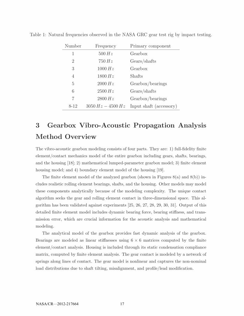
Table 1: Natural frequencies observed in the NASA GRC gear test rig by impact testing.

Number Frequency Primary component

1 500Hz Gearbox

2 750Hz Gears/shafts

3 1000Hz Gearbox

4 1800Hz Shafts

5 2000Hz Gearbox/bearings

6 2500Hz Gears/shafts

7 2800Hz Gearbox/bearings

8-12 3050Hz − 4500Hz Input shaft (accessory)

3 Gearbox Vibro-Acoustic Propagation Analysis

Method Overview

The vibro-acoustic gearbox modeling consists of four parts. They are: 1) full-fidelity finite

element/contact mechanics model of the entire gearbox including gears, shafts, bearings,

and the housing [18]; 2) mathematical lumped-parameter gearbox model; 3) finite element

housing model; and 4) boundary element model of the housing [19].

The finite element model of the analyzed gearbox (shown in Figures 8(a) and 8(b)) in-

cludes realistic rolling element bearings, shafts, and the housing. Other models may model

these components analytically because of the modeling complexity. The unique contact

algorithm seeks the gear and rolling element contact in three-dimensional space. This al-

gorithm has been validated against experiments [25, 26, 27, 28, 29, 30, 31]. Output of this

detailed finite element model includes dynamic bearing force, bearing stiffness, and trans-

mission error, which are crucial information for the acoustic analysis and mathematical

modeling.

The analytical model of the gearbox provides fast dynamic analysis of the gearbox.

Bearings are modeled as linear stiffnesses using 6 × 6 matrices computed by the finite

element/contact analysis. Housing is included through its static condensation compliance

matrix, computed by finite element analysis. The gear contact is modeled by a network of

springs along lines of contact. The gear model is nonlinear and captures the non-nominal

load distributions due to shaft tilting, misalignment, and profile/lead modification.

NASA/CR—2012-217664 17

Isolated finite element housing model is established in ANSYS. The housing excitation

source is dynamic bearing forces calculated using the finite element/contact or analytical

model. The surface velocity of the bearing is obtained by the dynamic responses. This

step can not be omitted because it connects the vibration analysis of the entire gearbox

and the housing noise radiation computation in the following step.

The full-fidelity boundary element model of the gearbox housing is established in the

software Coustyx [32, 19]. The acoustic model employees a multipole method ([32]) to

provide noise calculation with realistic housing dimensions. This housing surface velocity

calculated by ANSYS is inputted into the acoustic model as its boundary condition. This

acoustic model computes the radiated noise from the housing.

Major steps of the gearbox vibro-acoustic analysis is depicted in Figure 9.

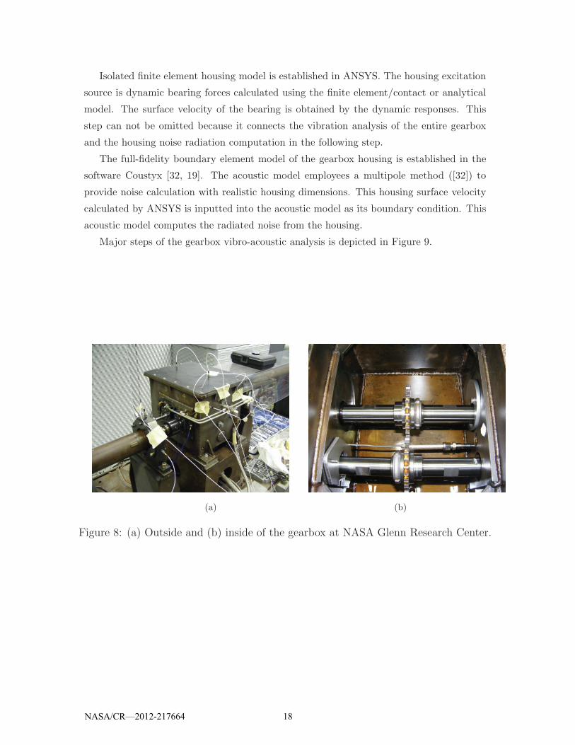
(a) (b)

Figure 8: (a) Outside and (b) inside of the gearbox at NASA Glenn Research Center.

NASA/CR—2012-217664 18

Finite Element Analysis

Analytical Analysis

Housing Vibration Analysis Acoustic Analysis

Transmission Error, Bearing Stiffness,Housing Compliance

Housing SurfaceVelocity

Dynamic BearingForces

1

......

..........

..

......

Figure 9: Key steps to perform the gearbox acoustic analysis.

4 Finite Element/Contact Mechanics Modeling and

Analysis of the Gearbox

4.1 Gearbox Modeling Overview

The examined NASA GRC gearbox (shown in Figures 8(a) and 8(b)) includes a pair of

spur gears with webbed rims, two staged shafts on which the gears are mounted, four

rolling element bearings that support the shafts, and the housing. The gear parameters

are listed in Table 3. Two types of rolling element bearings are used: cylindrical rolling

bearings and deep groove ball bearings (described in Table 2). Product designations are

SKF N205ECP and SKF 6205, respectively. The height and width of the gearbox housing

is 279.4mm and 254.0mm with 330.2mm length. The housing wall and lid thickness is

6.350mm. Details of the gearbox are described in [33, 24].

The realistic bearing model captures detailed bearing mechanics as shown in Figure 10,

including rolling elements, races, and the cage (not shown). This detailed bearing model

is used to determine the full 6×6 stiffness matrix between the shafts and housing. That

matrix is used in the mathematical gearbox model to perform fast dynamic simulations,

NASA/CR—2012-217664 19

Parameters (mm,degree) Cylindrical Roller Ball Bearing

Number of rows 1 1

Number of rolling elements 13 9

Contact angle 0 0

Pitch diameter 39.00 38.50

Bore diameter 25.00 25.00

Roller length 8.600 7.900

Roller diameter 7.500 7.900

Bearing width 15.00 15.00

Outer diameter 52.00 52.00

Outer diameter of inner raceway 31.50 34.40

Inner diameter of outer raceway 46.40 46.30

Radial clearance 40.00× 10−3 20.00× 10−3

Inner race crown curvature 10−7 0.520

Outer race crown curvature 10−7 0.520

Table 2: Single row cylindrical roller and ball bearing parameters.

as discussed later.

The gearbox housing is modeled by importing the full fidelity mesh established in

commercial finite element software, PATRAN. The housing is then assembled into the

gear/bearing/shaft system as shown in Figure 11.

4.1.1 Contact Solver

The contact solver of [18] seeks contact between gear teeth and bearing rolling elements

and raceways. Mesh stiffness variation, transmission error, tooth separation, and bearing

stiffness variation are inherently included; they are outputs rather than inputs. Transmis-

sion error is the major excitation source in geared systems [34] so an accurate transmission

error estimate is crucial. The finite element/contact analysis of the gearbox provides the

required reliable transmission error estimate.

The geometric surface descriptions of the contacting bodies must be precise to fully

address the contact characteristics. Additionally, the contact area is narrow and travels

over the entire body surface. Conventional finite element analysis requires a prohibitively

NASA/CR—2012-217664 20

(a) (b)

Figure 10: Cut-away finite element mesh of the radial ball bearing used in the gearbox (dimen-

sions detailed in Table 2) and a double-row cylindrical rolling element bearing (from a helicopter

application).

Parameters Values (mm, degree)

Number of teeth 28

Outer diameter 95.25

Root diameter 79.73

Facewidth 6.350

Module 3.175

Pressure angle 20

Center distance 88.90

Tooth thickness 4.851

Cutter edge radius 1.270

Linear tip relief 0.1778 starting at 24 degrees

Table 3: Dimensions of the spur gear pair

refined mesh to address these problems; a complete dynamic response analysis becomes

impossible in that case.

The finite element/contact mechanics model used here addresses these issues by using

a combination of the Boussinesq solution near the contacting surfaces and traditional finite

element analysis far away from the contact zones to exploit the advantages of each. The

details about this contact solver can be found in [35].

To accurately describe the contact area and pressure, the contact zone is discretized

into many small patches (grid cells). Sufficient number of grid cells within the contact

NASA/CR—2012-217664 21

Figure 11: Assembly of the gear-bearing-shaft-housing model.

zone is essential to obtain the correct contact pressure and load distribution. The finite

element model of the gear pair and contact pressure on individual tooth over a mesh cycle

are shown in Figure 12(a) and Figure 12(b). Figure 13(a) shows the finite element model

of a double-row cylindrical rolling element bearing. Contact patches on one of the radially

loaded cylinders are shown in Figure 13(b).

When the gears and rolling elements rotate, the number of teeth and rolling elements

in contact change, as do the location, size, and shape of the contact areas. These changes

are important as they affect bearing forces, gear tooth loads, and transmission error cal-

culations. The contact solver addresses these issues by determining and analyzing the

instantaneous gear and bearing contact conditions at every time instant.

This specialized finite element/contact mechanics software allows dynamic simulations

with greater modeling fidelity than conventional finite element tools. It is validated against

benchmark studies of complex gear dynamics problems [25, 26, 27, 28, 29, 30]. In exper-

imental comparisons, it has proven accurate in capturing the complex tooth mesh forces

leading to strong nonlinearity in the dynamics of single gear pairs [26], idler [29, 36], and

planetary gears [25, 27, 28, 37]. The rolling element contact in multiple bearings has been

validated against experiments in [31]. The shafts in the gearbox introduce system compli-

ance, could cause misalignment, and eventually affect transmission error. The accuracy of

the shaft models have been validated against classical beam theories as discussed later.

NASA/CR—2012-217664 22

(a) (b)

Figure 12: (a) Mating gears in the NASA GRC gearbox; (b) contact pressure on gear teeth over

one mesh cycle;

4.2 Fluid Film Wave Bearing Modeling

Bearings are critical components in geared systems. The fluid film wave bearings are

included in the gearbox model through the stiffness and damping matrices calculated by

the program developed by Hanford and Campbell [38, 39]. This wave bearing model uses

a perturbation method based on the Reynold equation to calculate the stiffness, damping,

pressure distribution, and load capacity of the fluid film. The program, however, is limited

to be two-dimensional by excluding the bearing tilting motion.

4.3 Rolling Element Bearing Modeling and Analysis

Theoretical bearing models [1, 40, 41, 42] make different assumptions to formulate the load-

deflection relation. These assumptions include different race elasticity, different property of

the rolling element contact, and ignoring microgeometry dimensions of bearing raceways.

Figure 14 shows the nonlinear stiffness-load relations of the cylindrical and radial ball

bearings calculated using the Harris [1], Gargiulo [2], and While [3] models. Significant

discrepancy is present among them.

The method developed to determine bearing stiffness does not make any assumptions

about the load-deflection relation. Instead, it calculates the 6× 6 bearing stiffness matrix

by partial derivatives of applied forces and moments related to six degrees of freedom. This

NASA/CR—2012-217664 23

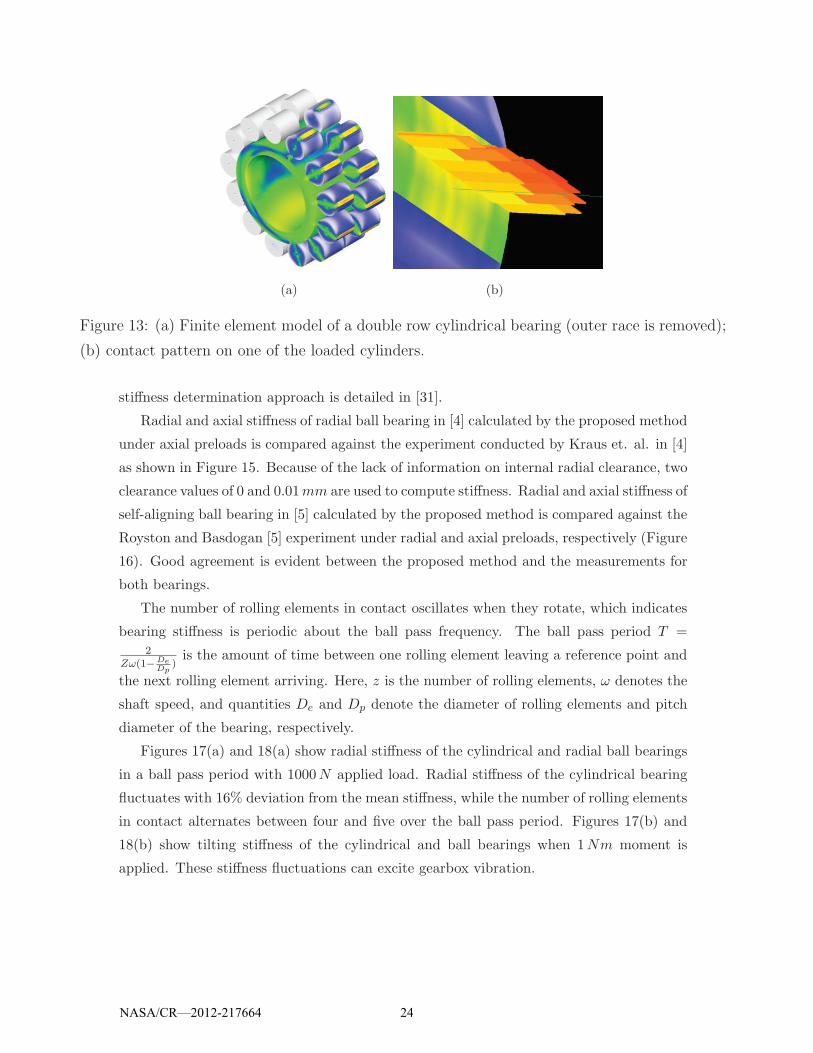
(a) (b)

Figure 13: (a) Finite element model of a double row cylindrical bearing (outer race is removed);

(b) contact pattern on one of the loaded cylinders.

stiffness determination approach is detailed in [31].

Radial and axial stiffness of radial ball bearing in [4] calculated by the proposed method

under axial preloads is compared against the experiment conducted by Kraus et. al. in [4]

as shown in Figure 15. Because of the lack of information on internal radial clearance, two

clearance values of 0 and 0.01mm are used to compute stiffness. Radial and axial stiffness of

self-aligning ball bearing in [5] calculated by the proposed method is compared against the

Royston and Basdogan [5] experiment under radial and axial preloads, respectively (Figure

16). Good agreement is evident between the proposed method and the measurements for

both bearings.

The number of rolling elements in contact oscillates when they rotate, which indicates

bearing stiffness is periodic about the ball pass frequency. The ball pass period T =2

Zω(1−DeDp

)is the amount of time between one rolling element leaving a reference point and

the next rolling element arriving. Here, z is the number of rolling elements, ω denotes the

shaft speed, and quantities De and Dp denote the diameter of rolling elements and pitch

diameter of the bearing, respectively.

Figures 17(a) and 18(a) show radial stiffness of the cylindrical and radial ball bearings

in a ball pass period with 1000N applied load. Radial stiffness of the cylindrical bearing

fluctuates with 16% deviation from the mean stiffness, while the number of rolling elements

in contact alternates between four and five over the ball pass period. Figures 17(b) and

18(b) show tilting stiffness of the cylindrical and ball bearings when 1Nm moment is

applied. These stiffness fluctuations can excite gearbox vibration.

NASA/CR—2012-217664 24

0 2 4 6 8 10

Radial load (kN)

Cylindrical Bearing

Ball Bearing

600

500

400

300

200

100

0

Ra

dia

l b

ea

rin

g s

tiffn

ess (

kN

/mm

)

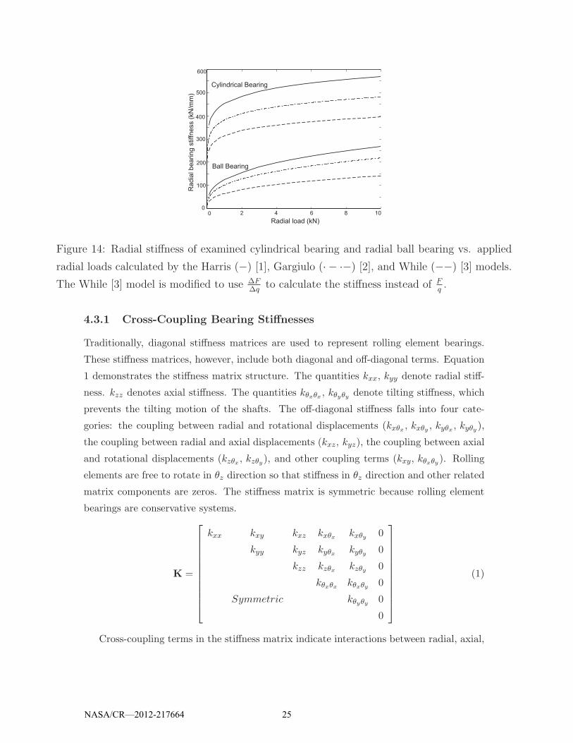
Figure 14: Radial stiffness of examined cylindrical bearing and radial ball bearing vs. applied

radial loads calculated by the Harris (−) [1], Gargiulo (· − ·−) [2], and While (−−) [3] models.

The While [3] model is modified to use ΔFΔq

to calculate the stiffness instead of Fq.

4.3.1 Cross-Coupling Bearing Stiffnesses

Traditionally, diagonal stiffness matrices are used to represent rolling element bearings.

These stiffness matrices, however, include both diagonal and off-diagonal terms. Equation

1 demonstrates the stiffness matrix structure. The quantities kxx, kyy denote radial stiff-

ness. kzz denotes axial stiffness. The quantities kθxθx , kθyθy denote tilting stiffness, which

prevents the tilting motion of the shafts. The off-diagonal stiffness falls into four cate-

gories: the coupling between radial and rotational displacements (kxθx , kxθy , kyθx , kyθy),

the coupling between radial and axial displacements (kxz, kyz), the coupling between axial

and rotational displacements (kzθx , kzθy), and other coupling terms (kxy, kθxθy). Rolling

elements are free to rotate in θz direction so that stiffness in θz direction and other related

matrix components are zeros. The stiffness matrix is symmetric because rolling element

bearings are conservative systems.

K =

⎡⎢⎢⎢⎢⎢⎢⎢⎢⎢⎢⎣

kxx kxy kxz kxθx kxθy 0

kyy kyz kyθx kyθy 0

kzz kzθx kzθy 0

kθxθx kθxθy 0

Symmetric kθyθy 0

0

⎤⎥⎥⎥⎥⎥⎥⎥⎥⎥⎥⎦

(1)

Cross-coupling terms in the stiffness matrix indicate interactions between radial, axial,

NASA/CR—2012-217664 25

50 100 150 200 250 300 350 4000

10

20

30

40

50

60

70

80

90

100

Axial load (N)

Ra

dia

l/a

xia

l st

iffn

ess

(k

N/m

m)

Radial stiffness

Axial stiffness

Figure 15: Comparison between the proposed method with zero (· · ·� · · · ) and 0.01mm (· −� · −) radial clearances and Kraus et al.’s [4] experiment (− ◦ −) for radial and axial stiffness

of the ball bearing in [4] under axial preloads.

and tilting motions of rolling element bearings. They demonstrate the coupling between

the shaft tilting motion, the flexural motion of the structure connected to the outer race,

and the shaft radial and axial motions. The effects of cross-coupling terms on the gearbox

vibration transmissibility through rolling element bearings are investigated. As the primary

excitation source, gear transmission error is an important measure of gearbox vibration.

Figure 19 shows the spectra of dynamic transmission error in the frequency range from 1500

to 4000Hz from numerical torque impulse cases. Bearing models with fully-populated and

diagonal stiffness matrices are compared as shown in Figure 19. Differences in resonant

frequencies and amplitudes are evident between these two bearing models. This stresses

the significance of the cross-coupling stiffnesses.

4.4 Gear Transmission Error

Transmission error is the major excitation source in geared systems. Accurate transmis-

sion error estimate is crucial. With the precise contact solver, the finite element/contact

analysis of the gearbox provides reliable transmission error estimate.

Transmission error is computed according to the tooth mesh deflection TE = (x1 −x2)sin(α) + (y1 − y2)cos(α) + r1θ1 + r2θ2, where xi, yi, θi, i = 1, 2 are the coordinates of

the mating gears as shown in Figure 20. α is the pressure angle and ri, i = 1, 2 are the

radii of the meshing gears. This formulation includes the shaft and bearing compliance.

NASA/CR—2012-217664 26

100 150 200 250 300 350 400 4500

10

20

30

40

50

60

70

80

90

100

Radial/axial load (N)

Ra

dia

l/a

xia

l st

iffn

ess

(k

N/m

m)

Radial stiffness, zero axial load

Axial stiffness, zero radial load

Figure 16: Comparison between the proposed method (· · ·� · · · ) and Royston and Basdogan [5]

experiment (− ◦ −) for radial and axial stiffness of self-aligning ball bearing in [5] under radial

and axial preloads, respectively.

Transmission error of this gear pair without shaft or bearing compliance has been com-

pared among Program X, Load Distribution Program, NASA DANST [43], and the current

approach in Figure 21. Program X is multi-body dynamics software that is used by in-

dustries worldwide. We are not free to state its name because of license restrictions for

academic use. The agreement on the peak to peak amplitude is reasonable. Differences

among the mean amplitudes are present. These differences are mainly caused by different

rim models these programs have used. Gear rims introduce compliance into the system,

leading to high amplitude of the mean transmission error. The current model includes the

realistic rim (as shown in Figure 12(a)). Others model the rims differently by excluding

the rim shoulders. Thus, their estimates of transmission error are lower. The Harris map

of transmission error at various torques is shown in Figure 22. The minimum transmis-

sion error without including the shaft compliance is at 67.79Nm torque, which matches

the torque the gear teeth are modified at. This further validates the transmission error

estimate.

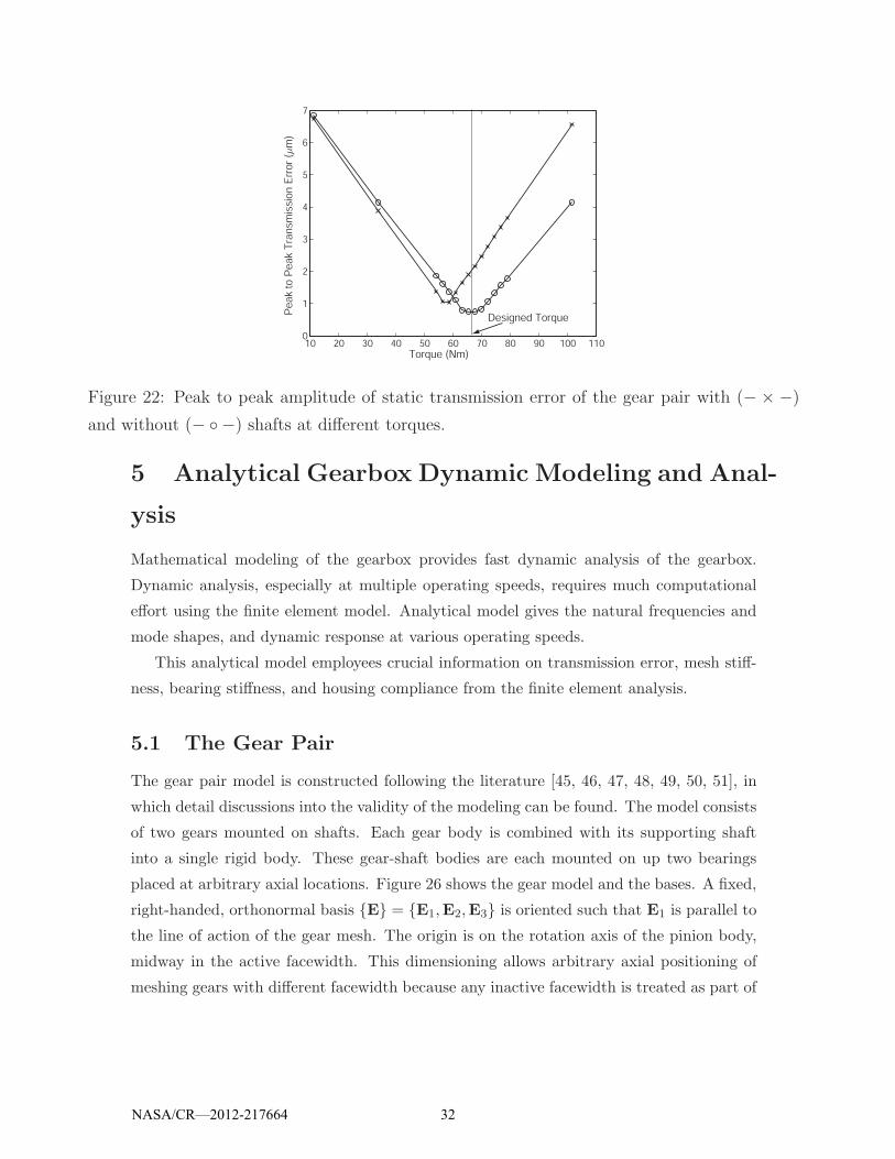
In addition, the minimum of the peak to peak value of transmission error is at lower

torque (57.62Nm) when flexible shafts are included as shown in Figure 22. This suggests

shaft compliance needs to be considered to estimate transmission error and modify gear

NASA/CR—2012-217664 27

160

240

170

180

190

200

210

220

230

0 0.2 0.4 0.6 0.8 1

Ball Pass Period

Rad

ial B

eari

ng

Sti

ffn

ess

(kN

/mm

)

0 0.2 0.4 0.6 0.8 1# o

f Ro

llers

in C

on

tact

5 5

4

Mean Stiffness

(a)

0.83

0.93

0.84

0.92

0.91

0.90

0.89

0.88

0.87

0.86

0.85

0 0.2 0.4 0.6 0.8 1

Ball Pass Period

Til

tin

g B

ea

rin

g S

tiff

ne

ss (

kN

m/r

ad

)

0 0.2 0.4 0.6 0.8 1# o

f R

oll

ers

in

Co

nta

ct

6 6 6

7 7

Mean Stiffness

(b)

Figure 17: (a) Radial and (b) tilting stiffness of the cylindrical bearing over a ball pass period.

The bottom figures show the number of rolling elements in contact over a ball pass period. The

applied load and moment are 1000N and 1Nm, respectively.

teeth.

4.5 Shaft Modeling and Validation

The long shafts in the gearbox introduce system compliance, could cause misalignment,

and eventually affect transmission error. The accuracy of the shaft models are important.

The shaft bending and torsional deformations are compared against classical beam

theories. The shaft bending model is considered as the elastic beam with a concentrated

load applied at the gear location. The beam bending boundary conditions are chosen as

simply-supported at each end of the shaft. The transverse deflection y along the shaft is

calculated as

y =Pb[x3−(L2−b2)x]3/2

6EIL , x < a

I =π(R4

out−R4in)

4

(2)

where the parameter P is the applied concentrated force. The parameters a, b are the

distances between one shaft end and the location where P is applied. The quantities

E, I, L denote the Young’s modulus, moment of inertia, and shaft length. The quantities

Rout, Rin denote the shaft outer and inner radii.

The analytical model to calculate the shaft torsional deflection has the clamped-free

NASA/CR—2012-217664 28

76

88

78

80

8282

84

86

0 0.2 0.4 0.6 0.8 1

Ball Pass Period

Rad

ial B

eari

ng

Sti

ffn

ess

(MN

/m)

0 0.2 0.4 0.6 0.8 1# o

f Ro

llers

in C

on

tact

5

4

5

Mean Stiffness

(a)

4.75

5.25

4.80

5.20

4.85

4.90

4.95

5.00

5.05

5.10

5.15

0 0.2 0.4 0.6 0.8 1

Ball Pass Period

Tilt

ing

Bea

rin

g S

tiff

nes

s (K

Nm

/rad

)

0 0.2 0.4 0.6 0.8 1

# o

f Ro

llers

in C

on

tact

4 4 4

3 3

Mean Stiffness

(b)

Figure 18: (a) Radial and (b) tilting stiffness of the ball bearing over a ball pass period. The

bottom figures show the number of rolling elements in contact over a ball pass period. The

applied load and moment are 1000N and 1Nm, respectively.

boundary condition. A torque T is applied at the free end of the shaft. The torsional

deflection θ is calculated asθ = Tx/GJ

G = E2(1+ν)

J = π2

(R4

out −R4in

)(3)

where the quantities ν, J denote the Possion’s ratio and the second moment of inertia.

Figures 23(a) and 23(b) show the shaft bending and torsional deformations calculated

by analytical solutions (solid line) and finite element results (square marker) at various

torques/forces. The finite element results of shaft bending and torsional deformations

agree with the analytical predictions.

In addition, as shown in Figure 4.5, the bending deformation is the same order of

magnitude of transmission error near the operating torque. Shaft deformation is significant.

Thus, including shafts would increase the overall accuracy of gearbox modeling.

NASA/CR—2012-217664 29

1500 1900 3300 3500 3900

10-2

10 -1

100

Frequency (Hz)

Dyn

am

ic t

ran

sm

issio

n e

rro

r

Inp

ut

torq

ue

(μm

/Nm

)L

og

(

)

37001700

Figure 19: Numerical torque impulse response of gear dynamic transmission error with fully-

populated (−) and diagonal (−−) stiffness matrices of the rolling element bearings mounted in

the examined gearbox based on [6]. The input torque equals 84.74Nm.

y

y

xx

αα

r r

θ

θ

o o

1

1

1

1

1

2

2

2

2

2

Line of Action

Figure 20: Coordinates of the examined gear pair.

4.6 Dynamic Analysis and Correlation with Experiments

Modal analysis is performed numerically on the gearbox model by applying a torque im-

pulse at the input shaft and measuring the dynamic response. Numerical impulse test

provides natural frequencies and mode shapes of the gearbox. Results of the impulse test

are correlated with experimental measurements conducted by NASA personnel [44] and

the Ohio State research group.

The frequency spectrum of dynamic transmission error and shaft displacement for the

speed range from 0 to 8000Hz are shown in Figures 25(a) and 25(b). The computed

natural frequencies agree with experiments as compared in Table 4. NASA accelerometers

identify natural frequencies near 3000 to 4500Hz, but the coherence is relatively low at

NASA/CR—2012-217664 30

0 0.2 0.4 0.6 0.8 110

12

14

16

18

20

22

24

26

28

30

Mesh Cycle

Sta

tic T

rans

mis

sion

Err

or (μ

m)

Figure 21: Static transmission error of the gear pair without the shaft and bearing compliance.

The results are calculated by finite element (−), Program X (− · −), NASA DANST (· · · ), andLoad Distribution Program (−−). The torque equals 79.09Nm.

these higher frequencies. Measurements show several modes near 6500 to 7500Hz that

are difficult to resolve, while simulations predict only one natural frequency at 6856Hz.

The mode shapes of these natural frequencies include mesh deflection modes, shaft modes,

housing modes, and coupled modes.

Finite Element Experiment

759 750

1942 2000

2195, 2283 2500

3803, 4449, 4654 3000-4500

6856 6500-7500

Table 4: Natural frequencies predicted by numerical impulse tests and measurements (Hz)

NASA/CR—2012-217664 31

10 20 30 40 50 60 70 80 90 100 1100

1

2

3

4

5

6

7

Torque (Nm)

Pea

k to

Pea

k T

rans

mis

sion

Err

or (μ

m)

Designed Torque

Figure 22: Peak to peak amplitude of static transmission error of the gear pair with (− × −)

and without (− ◦ −) shafts at different torques.

5 Analytical Gearbox Dynamic Modeling and Anal-

ysis

Mathematical modeling of the gearbox provides fast dynamic analysis of the gearbox.

Dynamic analysis, especially at multiple operating speeds, requires much computational

effort using the finite element model. Analytical model gives the natural frequencies and

mode shapes, and dynamic response at various operating speeds.

This analytical model employees crucial information on transmission error, mesh stiff-

ness, bearing stiffness, and housing compliance from the finite element analysis.

5.1 The Gear Pair

The gear pair model is constructed following the literature [45, 46, 47, 48, 49, 50, 51], in

which detail discussions into the validity of the modeling can be found. The model consists

of two gears mounted on shafts. Each gear body is combined with its supporting shaft

into a single rigid body. These gear-shaft bodies are each mounted on up two bearings

placed at arbitrary axial locations. Figure 26 shows the gear model and the bases. A fixed,

right-handed, orthonormal basis {E} = {E1,E2,E3} is oriented such that E1 is parallel to

the line of action of the gear mesh. The origin is on the rotation axis of the pinion body,

midway in the active facewidth. This dimensioning allows arbitrary axial positioning of

meshing gears with different facewidth because any inactive facewidth is treated as part of

NASA/CR—2012-217664 32

50 100 150 200 250 300 3500

10

20

30

40

50

60

70

80

90

Shaft Length (mm)

Sha

ft B

endi

ng D

efor

mat

ion

(μm

)

33.90 Nm

84.74 Nm

101.7 Nm

(a)

50 100 150 200 250 300 3500

0.5

1

1.5

2

2.5

3

3.5

4

Shaft Length (mm)

Sha

ft T

orsi

onal

Def

orm

atio

n (

radi

ans)

101.7 Nm

84.74 Nm

33.90 Nm

10-3

(b)

Figure 23: (a) Input shaft bending deformation calculated by analytical beam theory (solid line)

and finite element method (square marker) with simply-supported boundary conditions under

various input torques; (b) Input shaft torsional deformation calculated by analytical beam theory

(solid line) and finite element method (square marker) with clamped-free boundary conditions

under various input torques. The shaft has uniform outer diameter (30.23mm).

the shaft. The translational (xp, yp, zp) and angular (φp, θp, βp) coordinates of the pinion

body are assigned to translations along and rotations about E1, E2, and E3, respectively.

The translational and angular coordinates of the gear body follow similarly with subscript

g. Body-fixed bases {ep} = {ep1, ep2, ep3} and {eg} = {eg1, eg2, eg3} for the pinion and gear are

adopted. Positive axial quantities are measured along E3 from the dashed line in Figure

26.

The pinion translational and angular velocity vectors are

rp = xpE1 + ypE2 + zpE3,

ωp =[φp − θp

(βp +Ωp

)]ep1 +

[θp + φp

(βp +Ωp

)]ep2 +

[βp +Ωp − φpθp

]ep3,

(4)

where Ωp is the constant angular rotational speed of the pinion. The velocity vectors for

the gear are identical except with components for the gear.

The pinion body is supported by two bearings at points Ap and Bp. The axial positions

of these bearings measured along E3 are LAp and LB

p . The pinion bearing deflection vectors

at point Ap and Bp are the relative deflections of points Ap and Bp with respect to ground,

NASA/CR—2012-217664 33

100 150 200 250 3000

10

20

30

40

50

60

70

80

90

Shaft Length (mm)

Ma

gn

itu

de

of

Sh

aft

Be

nd

ing

(μm

)

101.7 Nm

79.09 Nm

33.90 Nm

Figure 24: Shaft bending deformation under various input torques.

giving

dAp =

[θp(LAp − ep

)+ xp

]E1 +

[φp(ep − LA

p

)+ yp

]E2 + zpE3,

dBp =

[θp(LBp − ep

)+ xp

]E1 +

[φp(ep − LB

p

)+ yp

]E2 + zpE3.

(5)

The bearing deflections for the gear follow similarly. The bearings resist tilting as well.

The angular deflection of the pinion body bearing at Ap is

γAp = φpE1 + θpE2 + βpE3. (6)

The angular bearing deflection at point Bp is identical to Eq. (6) for rigid shafts. The

bearings are isotropic in the E1 −E2 plane. At point Ap, the bearing stiffness matrix KAp

as given in Eq. (1) is fully-populated, where the equality of stiffness in the two translation

directions is evident. The bearing translational and angular displacements combined are

Γ ={dγ

}. Similar definitions follow for point Bp and for the gear body.

The gear mesh interface is modeled by a series of springs along the nominal lines of

contact for no mesh deflection. These lines change as the gears rotate. Each spring acts

at a point denoted by Ci. When the gear bodies deflect, the contact points on the pinion

separate or compress against the contact points on the gear. The difference between

the position vectors of the contact points on the pinion and gear gives the relative mesh

deflection vector at Ci. The projection of the relative mesh deflection vector on the tooth

surface normal gives the relative compressive deflection at the ith contact point. The

NASA/CR—2012-217664 34

1000 2000 3000 4000 5000 6000 7000 80000

0.1

0.2

0.3

0.4

0.5

0.6

0.7

Frequency (Hz)

2195Hz

4449Hz

3803Hz6856Hz

Dy

na

mic

tra

nsm

issi

on

err

or

Inp

ut

torq

ue

(μm

/Nm

)

(a)

1000 2000 3000 4000 5000 6000 7000 80000

0.5

1

1.5

2

2.5

3

3.5

4

4.5

Frequency (Hz)

759Hz

Sh

aft

Ve

rtic

al

Dis

pla

ce

me

nt

Inp

ut

torq

ue

(μm

/Nm

)

1942Hz

2283Hz

3865Hz

4654Hz

5806Hz

(b)

Figure 25: Numerical impulse test results of (a) dynamic transmission error and (b) the input

shaft horizontal displacement of the gear-bearing-housing system within speed range from 0Hz

to 7000Hz. The applied torque is 79.09Nm.

relative compressive deflection is

δi(q, t) ={[ep − ci(t)] θp + [ci(t)− eg] θg − xp + xg + hi + βprp + βgrg

}cosψ

−{[bi(t) + hi] θp + [(rp + rg) θg tanΦ− bi(t)] + zp − zg + φprp + φgrg

}sinψ,

(7)

where rp and rg are the base radii, Φ is the transverse operating pressure angle, and ψ is

the base helix angle. The vector q comprises generalized coordinates

q =(φp, θp, βp, xp, yp, zp︸ ︷︷ ︸

pinion

, φg, θg, βg, xg, yg, zg︸ ︷︷ ︸gear

)(8)

The axial position of a contact point is ci(t) measured from the origin along E3, and the

transverse position of a contact point is bi(t) measured from the origin along −E1. They

are known functions of time determined by the contact line progressions as the gears rotate.

Micron-level deviations of the tooth surface from an involute at any contact point i, such

as from gear tooth surface modifications and manufacturing errors, are denoted by hi.

Figures 26 and 27(b) depict these quantities.

NASA/CR—2012-217664 35

Gear

rp

bi

Pinion

Pinion

Gear

Ag

LgA

ep

rg

ge

2

ge

1

Contact

points Ci

Bg

Ap Bp E1

E3

ci

eg

LgB

LpA Lp

B

Φpx

gx

gy

E2

Φ

Contact

points Ci

Figure 26: Analytical model of the gear pair. The parameters are defined in [7]. The dashed

line is at the center of the active facewidth.

The kinetic and potential energies are

T =1

2

(ωT

p Jpωp + ωTg Jgωg + rTpmprp + rTgmg rg

),

V =1

2

[ΓApTKA

p ΓAp + ΓB

pTKB

p ΓBp + ΓA

pTKA

GΓAp + ΓB

pTKB

GΓBp

]

+1

2

n(t)∑i=1

ki(q, t)δi(q, t)2,

(9)

where ki(q, t) is the ith contact stiffness, and n(t) is the number of contact segments at

an instant t. These quantities change as the gears rotate, hence the time dependence.

The inertia tensor of the axisymmetric pinion body is Jp = diag[Jxp , J

xp , J

zp

]with similar

definition for the axisymmetric gear body.

Lagrange’s equations of motion for unconstrained generalized coordinates follow after

substitution of equations Eqs. (4) through (7) into the energy expressions Eq. (9). In

matrix form they are

Msqs +Dqs +ΩpGsqs +[Ks(q, t)− Ω2

pCs

]q = F(q, t)s, (10)

The vector F includes external loading; the driving and absorbing torques and tooth surface

modifications hi appear here. The matrix K represents the system elasticity with losses

contained in the modal damping matrix D. Tooth surface modifications hi are neglected

in K because hi � bi(t), and the hi appear as additions to bi(t). The terms that arise from

NASA/CR—2012-217664 36

kb

kc

ψl(t)

Gear

Pinion

{{hi

Contact point Ci

(a)

Gear

Pinion

ki

bici

Contact point Ci

{hi

(b)

Figure 27: (a) Distributed spring network over a contact line with the local and bulk stiffnesses,

kcl(t) and kb. (b) Local kcl(t) and bulk kb stiffnesses are combined into contact stiffness ki(q, t)

by Eq. (14).

the constant rotation speed are contained in the gyroscopic matrix G and the centripetal

acceleration matrix C. Individual elements of M, K, G, C, and f are given in [7].

Following [52, 50] the nominal contact lines are discretized into n(t) segments of equal

length l(t), as shown in Figure 27(a). Each contact point Ci is positioned at the center of

its segment. As the contact lines progress with gear rotation, the total number of segments

n(t) and the length of a segment l(t) change. Each contact line has a specified number

of segments. This discretization is based on the nominal lines of contact with no gear

deflections.

Each contact spring is attached to its contact point Ci. The stiffness ki(q, t) of contact

springs are obtained by considering two separate categories of tooth deflection: local (εi)

and bulk (δb). Discussion of this categorization can be found in [52, 49, 53]. The local

deflection represents the Hertz contact deflections. The associated local stiffness is kcl(t),

where the constant kc is the local stiffness per unit contact length. The bulk deflection

represents all deflections except local deflection, and those include gear blank deflection,

tooth bending, shear, etc. Because the Hertz contact deflections are localized and far

enough from the bulk deflections, the bulk deflection is assumed to be the same for all

contact segments. The bulk stiffness kb is assumed constant. The bulk spring is in series

with the local springs, so the total deflection at the ith contact point Ci is

δi = εi + δb (11)

The mesh force F equals the sum of all forces carried by the local springs and also the

NASA/CR—2012-217664 37

force carried by the bulk spring due to the series connection. The mesh force is

F =

n∑i=1

Fi = kcl(t)

n∑i=1

εiH(εi) = kbδb, (12)

H(εi) =

{1; εi ≥ 0

0; εi < 0(13)

is the Heaviside function that represents the contact condition at each contact spring. Use

of Eqs. (11) and (12) reduce the network of local and bulk springs into n(t) contact springs

(ki, i = 1, 2, . . . , n) in parallel, as shown in Figure 27(b). The ith contact stiffness is given

by

ki(q, t) =kbkcl(t)H(εi)

kb + kcl(t)

n(t)∑i=1

H(εi)

. (14)

One can then calculate the ith potential energy kiδ2i /2 stored in the gear mesh in Eq. (9)

from the contact force Fi = kiδi.

The local stiffness per unit length kc and the bulk stiffness kb are parameters of the

gear pair determined by the contact mechanics and elasticity of the gears. These constants

can be approximated analytically [52] or semi-analytically [50] by assigning certain types

of stiffnesses such as Hertz contact, tooth bending, shear, etc. to kc and kb. A different

approach is used in this work, where kc and kb are solved for from the deflections obtained

from an external analysis tool for computational static analyses. In this case, kc and kb are

numerical values that best fit the deflection obtained from finite element contact analysis

of gears.

The following stipulations simplify the algebra to find kc and kb. 1) The tooth surface

is perfectly involute, that is, hi = 0 for all i; 2) All degrees of freedom are constrained

to be zero except the pinion rotation βp; and 3) A specified moment about E3 is applied

to the pinion. With these stipulations, the deflections at all contact points are identical,

that is, δi = δ for all i in Eq. (7). Consequently, all points are in contact; Hi = 1 for

all i. The subscript i of ki is unnecessary because when all segments are in contact,

k1 = k2 = . . . = kn. Use of static equilibrium, Eq. (11), and Eq. (14) gives

δ(t) = F

[1

kb+

1

kcL(t)

], (15)

where δ(t) is the static transmission error, L(t) = n(t)l(t) is the total contact line length

at an instant t, and F is the constant mesh force obtained from the known applied torque.

The two unknowns (kc, kb) are solved using the data from finite element analysis results

NASA/CR—2012-217664 38

at two instances {δ(t1), L(t1)} and {δ(t2), L(t2)} within a mesh cycle. To increase accu-

racy, values at these two instances are calculated from averages of the four points where

transmission error is highest (giving the values for the first instance) and the four points

where transmission error is lowest (giving the values for the second instance).

The gear mesh model is validated by finite element analysis. Figure 28 shows trans-

mission error comparison between the finite element and the analytical model for a helical

and a spur gear pair.

0 T/4 T/2 3T/4 T6

6.5

7

7.5

Gear Mesh Cycle

Tra

nsm

issio

n E

rror

[μm

]

FEA

Analytical

(a)

0 T/4 T/2 3T/4 T

20

22

24

Gear Mesh Cycle

Analytical

FEA

Tra

nsm

issio

n E

rror

[μm

]

(b)

Figure 28: Static transmission error from the analytical (solid line) and finite element (circles)

model. (a) A helical gear pair. Quadratic tip relief starting at α = 28 deg and root relief at

α = 27 deg. Tip relief, root relief, and circular lead crown are 10 μm. The applied torque is

200 N-m. (b) Spur gear pair in [8]. Linear tip relief starting at α = 23.6 deg with amplitude 10

μm. Circular lead crown is 5 μm. The applied torque is 340 N-m.

5.2 Incorporating Housing Compliance with the Analytical

Gear/Shaft Model

The equations of motion for the housing is given by

MH qH +KHqH = FH (16)

where MH and KH are the mass and the stiffness matrices with degrees of freedom qH

and the force vector fH . Figure 29 helps explain the approach. The gear/shaft equations

of motion are expanded by the addition of bearing degrees of freedom qb and the housing

equation of motion by Partitioning of (16) to separate the degrees of freedom where the

NASA/CR—2012-217664 39

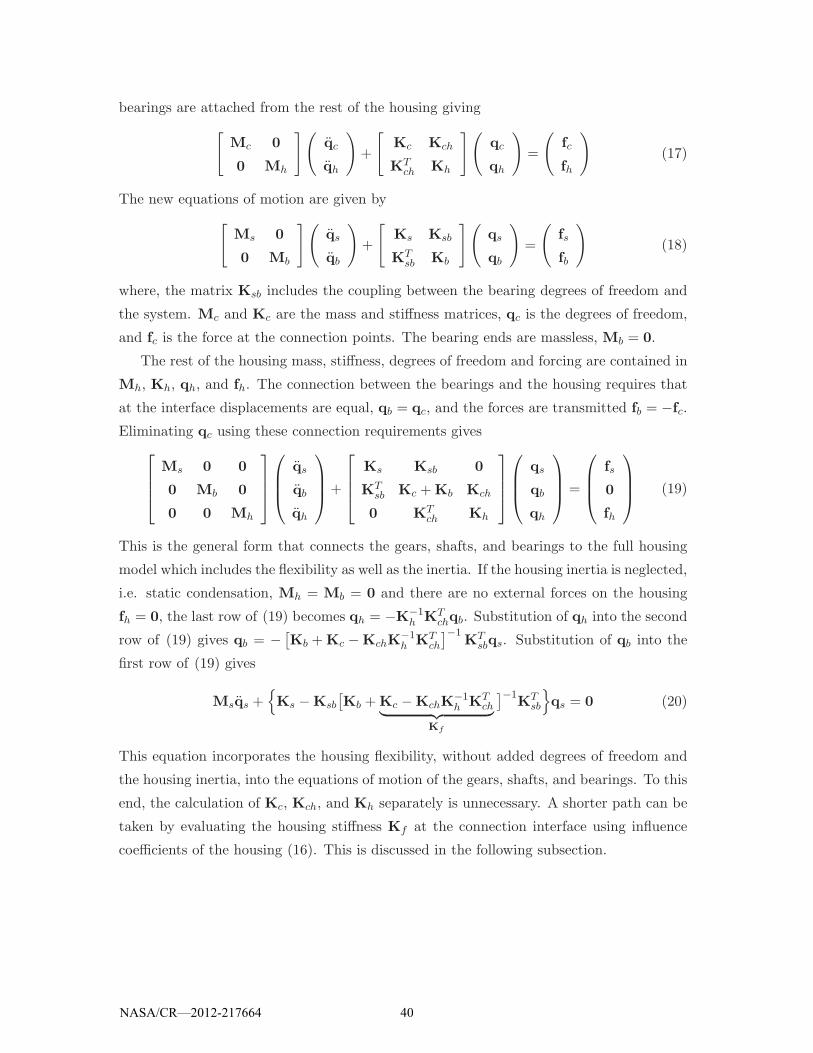
bearings are attached from the rest of the housing giving[Mc 0

0 Mh

](qc

qh

)+

[Kc Kch

KTch Kh

](qc

qh

)=

(fc

fh

)(17)

The new equations of motion are given by[Ms 0

0 Mb

](qs

qb

)+

[Ks Ksb

KTsb Kb

](qs

qb

)=

(fs

fb

)(18)

where, the matrix Ksb includes the coupling between the bearing degrees of freedom and

the system. Mc and Kc are the mass and stiffness matrices, qc is the degrees of freedom,

and fc is the force at the connection points. The bearing ends are massless, Mb = 0.

The rest of the housing mass, stiffness, degrees of freedom and forcing are contained in

Mh, Kh, qh, and fh. The connection between the bearings and the housing requires that

at the interface displacements are equal, qb = qc, and the forces are transmitted fb = −fc.

Eliminating qc using these connection requirements gives⎡⎢⎢⎣

Ms 0 0

0 Mb 0

0 0 Mh

⎤⎥⎥⎦⎛⎜⎜⎝

qs

qb

qh

⎞⎟⎟⎠+

⎡⎢⎢⎣

Ks Ksb 0

KTsb Kc +Kb Kch

0 KTch Kh

⎤⎥⎥⎦⎛⎜⎜⎝

qs

qb

qh

⎞⎟⎟⎠ =

⎛⎜⎜⎝

fs

0

fh

⎞⎟⎟⎠ (19)

This is the general form that connects the gears, shafts, and bearings to the full housing

model which includes the flexibility as well as the inertia. If the housing inertia is neglected,

i.e. static condensation, Mh = Mb = 0 and there are no external forces on the housing

fh = 0, the last row of (19) becomes qh = −K−1h KT

chqb. Substitution of qh into the second

row of (19) gives qb = − [Kb +Kc −KchK−1h KT

ch

]−1KT

sbqs. Substitution of qb into the

first row of (19) gives

Msqs +{Ks −Ksb

[Kb +Kc −KchK

−1h KT

ch︸ ︷︷ ︸Kf

]−1KT

sb

}qs = 0 (20)

This equation incorporates the housing flexibility, without added degrees of freedom and

the housing inertia, into the equations of motion of the gears, shafts, and bearings. To this

end, the calculation of Kc, Kch, and Kh separately is unnecessary. A shorter path can be

taken by evaluating the housing stiffness Kf at the connection interface using influence

coefficients of the housing (16). This is discussed in the following subsection.

NASA/CR—2012-217664 40

Gears & shafts

Mh,Kh

xb

Ms,Ks

Mc, Kc

Bearings

Housing

Kb

xc

Connection

xs

Figure 29: Description of the connection between the gears, shafts and bearings to the housing

model.

5.2.1 Including the Housing by Using Influence Coefficients

The influence coefficient matrix Cf can be solved from (16) Cf fc = qc Solving for qh

from (17) gives

C−1f = Kf = Kc −KchK

−1h KT

ch (21)

which allows use of the influence coefficient matrix in (20).

The procedure to obtain elements of Cn×nf consists of applying a unit force to each

degree of freedom at the connection points fc one at a time, and measuring the deflection

of all the degrees of freedom at the connection points qc. Explicitly, elements in the ith

column, C<i><j>f , are given by the displacements q<j>

c , calculated by (16) when there is

a unit force at f<i>c = 1, where j = 1, . . . , n.

5.3 Dynamic Analysis Using the Analytical Model

Table 5 shows the natural frequencies of four systems: 1) cylindrical/ball bearings with

housing flexibility, 2) wave bearings with housing flexibility, 3) cylindrical/ball bearings

without housing flexibility, and 4) wave bearings without housing flexibility. Figure 30

shows the mesh deflection mode from the analysis with cylindrical/ball bearings with

housing flexibility. The mesh deflection mode is an important mode because the tooth

pass excitation excites primarily the mesh deflection mode. This mesh deflection mode is

demonstrated in experiments, which is strongly excited by the 2nd harmonic of tooth pass

frequency at 4200rpm. This mode shows up strongly in our vibration speed maps. It is

NASA/CR—2012-217664 41

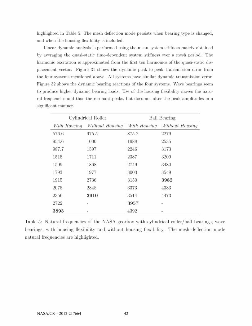
highlighted in Table 5. The mesh deflection mode persists when bearing type is changed,

and when the housing flexibility is included.

Linear dynamic analysis is performed using the mean system stiffness matrix obtained

by averaging the quasi-static time-dependent system stiffness over a mesh period. The

harmonic excitation is approximated from the first ten harmonics of the quasi-static dis-

placement vector. Figure 31 shows the dynamic peak-to-peak transmission error from

the four systems mentioned above. All systems have similar dynamic transmission error.

Figure 32 shows the dynamic bearing reactions of the four systems. Wave bearings seem

to produce higher dynamic bearing loads. Use of the housing flexibility moves the natu-

ral frequencies and thus the resonant peaks, but does not alter the peak amplitudes in a

significant manner.

Cylindrical Roller Ball Bearing

With Housing Without Housing With Housing Without Housing

576.6 975.5 875.2 2279

954.6 1000 1988 2535

987.7 1597 2246 3173

1515 1711 2387 3209

1599 1868 2749 3480

1793 1977 3003 3549

1915 2736 3150 3982

2075 2848 3373 4383

2356 3910 3514 4473

2722 - 3957 -

3893 - 4392 -

Table 5: Natural frequencies of the NASA gearbox with cylindrical roller/ball bearings, wave

bearings, with housing flexibility and without housing flexibility. The mesh deflection mode

natural frequencies are highlighted.

NASA/CR—2012-217664 42

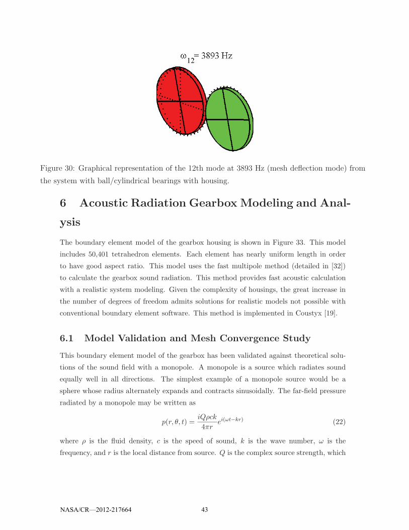
Figure 30: Graphical representation of the 12th mode at 3893 Hz (mesh deflection mode) from

the system with ball/cylindrical bearings with housing.

6 Acoustic Radiation Gearbox Modeling and Anal-

ysis

The boundary element model of the gearbox housing is shown in Figure 33. This model

includes 50,401 tetrahedron elements. Each element has nearly uniform length in order

to have good aspect ratio. This model uses the fast multipole method (detailed in [32])

to calculate the gearbox sound radiation. This method provides fast acoustic calculation

with a realistic system modeling. Given the complexity of housings, the great increase in

the number of degrees of freedom admits solutions for realistic models not possible with

conventional boundary element software. This method is implemented in Coustyx [19].

6.1 Model Validation and Mesh Convergence Study

This boundary element model of the gearbox has been validated against theoretical solu-

tions of the sound field with a monopole. A monopole is a source which radiates sound

equally well in all directions. The simplest example of a monopole source would be a

sphere whose radius alternately expands and contracts sinusoidally. The far-field pressure

radiated by a monopole may be written as

p(r, θ, t) =iQρck

4πrei(ωt−kr) (22)

where ρ is the fluid density, c is the speed of sound, k is the wave number, ω is the

frequency, and r is the local distance from source. Q is the complex source strength, which

NASA/CR—2012-217664 43

0 1000 2000 3000 4000 50000

5

10

15

20

25

30

PP T

E [µ

m]

Frequency [Hz]

B/nHB/HW/nHW/H

Figure 31: Peak-to-peak dynamic transmission error of four systems. Analysis with roller ele-

ment bearings are marked by B, analysis with wave bearings are marked by W, analysis including

the housing flexibility is marked by H, analysis without the housing is marked by nH.

is a constant number defined in [54].

The sound field excited by a monopole is not affected by the gearbox geometry, which

allows simulation results to be compared against the theoretical solution of a monopole

for an arbitrary geometry. In other words, the noise radiation from the gearbox surface

equals to the theoretical solution of a monopole in the free space (shown in Figure 34).

The velocity field caused by the point source (monopole) in free space at gearbox surface is

calculated theoretically and used as the boundary condition for the actual housing model.

Optimal element length has been carefully chosen through mesh convergence study.

The relative error of the computed pressure compared to the theoretical value in (22)

with various element length is shown in Figure 35. Result accuracy is improved when

element length is small. However, when element length is smaller than 8.636mm, the

result accuracy is disrupted as round off error becomes significant. The optimal element

length is between 8.890mm and 10.16mm with less than 2% relative error. The mesh

convergence study is important as the element length affects the solution accuracy.

Sound pressure of the radiated noise calculated by Coustyx and the theoretical solution

is compared in Figure 36 for the speed range from 500 to 3500Hz using 9.000mm element

length. Excellent agreement is present.

NASA/CR—2012-217664 44

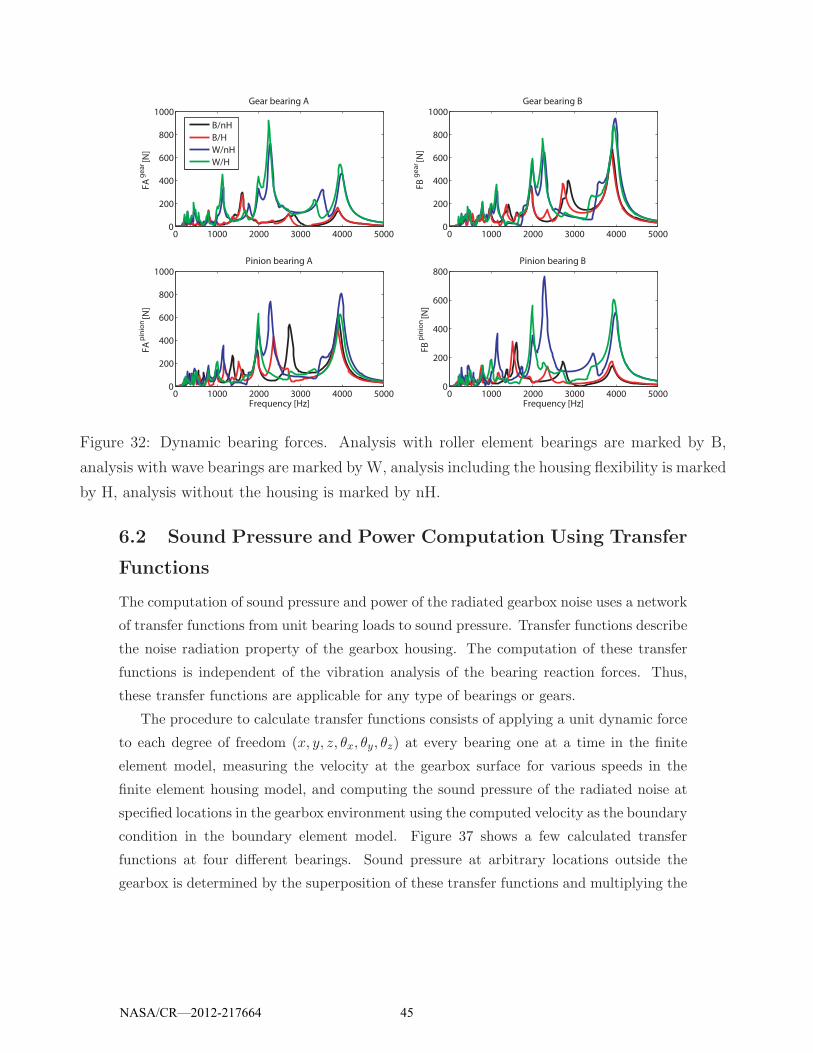
0 1000 2000 3000 4000 50000

200

400

600

800

1000

FA

ge

ar [

N]

Gear bearing A

0 1000 2000 3000 4000 50000

200

400

600

800

1000

FB

ge

ar [

N]

Gear bearing B

0 1000 2000 3000 4000 50000

200

400

600

800

1000

FA

pin

ion [

N]

Frequency [Hz]

Pinion bearing A

0 1000 2000 3000 4000 50000

200

400

600

800

FB

pin

ion [

N]

Pinion bearing B

Frequency [Hz]

B/nH

B/H

W/nH

W/H

Figure 32: Dynamic bearing forces. Analysis with roller element bearings are marked by B,

analysis with wave bearings are marked by W, analysis including the housing flexibility is marked

by H, analysis without the housing is marked by nH.

6.2 Sound Pressure and Power Computation Using Transfer

Functions

The computation of sound pressure and power of the radiated gearbox noise uses a network

of transfer functions from unit bearing loads to sound pressure. Transfer functions describe

the noise radiation property of the gearbox housing. The computation of these transfer

functions is independent of the vibration analysis of the bearing reaction forces. Thus,

these transfer functions are applicable for any type of bearings or gears.

The procedure to calculate transfer functions consists of applying a unit dynamic force

to each degree of freedom (x, y, z, θx, θy, θz) at every bearing one at a time in the finite

element model, measuring the velocity at the gearbox surface for various speeds in the

finite element housing model, and computing the sound pressure of the radiated noise at

specified locations in the gearbox environment using the computed velocity as the boundary

condition in the boundary element model. Figure 37 shows a few calculated transfer

functions at four different bearings. Sound pressure at arbitrary locations outside the

gearbox is determined by the superposition of these transfer functions and multiplying the

NASA/CR—2012-217664 45

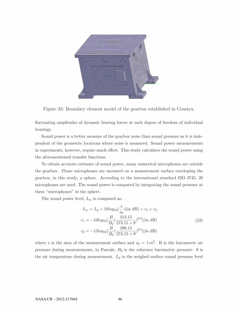
Figure 33: Boundary element model of the gearbox established in Coustyx.

fluctuating amplitudes of dynamic bearing forces at each degree of freedom of individual

bearings.

Sound power is a better measure of the gearbox noise than sound pressure as it is inde-

pendent of the geometric locations where noise is measured. Sound power measurements

in experiments, however, require much effort. This study calculates the sound power using

the aforementioned transfer functions.

To obtain accurate estimate of sound power, many numerical microphones are outside

the gearbox. Those microphones are mounted on a measurement surface enveloping the

gearbox, in this study, a sphere. According to the international standard ISO 3745, 20

microphones are used. The sound power is computed by integrating the sound pressure at

these “microphones” in the sphere.

The sound power level, Lw is computed as:

Lw = Lp + 10log10(s

s0)(in dB) + c1 + c2

c1 = −10log10[B

B0(

313.15

273.15 + θ)0.5](in dB)

c2 = −15log10[B

B0(

296.15

273.15 + θ)0.5](in dB)

(23)

where s is the area of the measurement surface and s0 = 1m2. B is the barometric air

pressure during measurements, in Pascals; B0 is the reference barometric pressure. θ is

the air temperature during measurement. Lp is the weighed surface sound pressure level

NASA/CR—2012-217664 46

Microphone

Monopole

Theoretical Boundary Condition Excited by Monopole

Figure 34: Theoretical solutions used to validate the boundary element housing model. Noise

radiated from the housing with monopole velocity field at the gearbox surface as the boundary

condition equals to that with monopole in the free space.

over the measurement surface in decibels.

Lp = 10log10{( 1N

[∑i

100.1(Lp,i+W )])}in dB

Lp,i = 20log10(pip0

)

(24)

where N is the number of microphone positions. W is the weighting function applied

by the filter at the frequency of analysis. pi is the root mean square pressure in Pa and

p0 = 2× 10−5 Pa.

6.3 Radiated Noise Correlation with Measurements

The calculated noise is compared against the measurements taken at NASA GRC gearbox.

Two microphones are mounted to measure sound pressure in experiments at 790 mm

directly above the gearbox, and are separated horizontally by 180 mm as shown in Figure

38.

Here, only the noise transmitted through rolling element bearings are compared against

measurements because experimental data on sound pressure with wave bearings is not

available. Figure 39 shows the time averages of the mean squared sound pressure (p)2av =∑b (pb)

2av at microphone 1 estimated by measurements and computed, where (pb)av

2 is

the addictive measure of sound pressure associated with the frequency band b from 0 to

NASA/CR—2012-217664 47

7 8 9 10 11 12 130

1

2

3

4

5

6

Boundary Element Length (mm)

Per

cent

age

of R

elat

ive

Err

or, S

ound

Pre

ssur

e

Figure 35: Effects of boundary element length on the relative error of calculated sound pressure

compared to the theoretical solution.

8000Hz. For each gear mesh frequency, two different experimental results are shown:

the minimum sound pressure including only mesh frequency harmonics; and the maxi-

mum sound pressure including mesh frequency harmonics and other frequency components.

These frequencies are the side bands caused by the shaft rotation frequency, belt splice

pass frequency, etc. The simulated sound pressure is within the experimental data range.

Figure 40 shows the frequency spectrum of the measured and simulated sound pressure

when mesh frequency equals 2000Hz. Good agreement is evident between the measure-

ments and simulations at mesh frequency harmonics. Sidebands around the mesh frequency

harmonics are present in the measured data. These sidebands are not included in the com-

putational model because the causes are not known. Including these sidebands in the

vibration/acoustics model would provide better agreement with the measurements.

NASA/CR—2012-217664 48

500 1000 1500 2000 2500 3000 3500-20

-15

-10

-5

0

5

10

15

20

Frequency (kHz)

Sou

nd p

ress

ure,

rea

l par

t (P

a)

Figure 36: Sound pressure at the NASA microphone 1 location calculated by Coustyx (�) and

theoretical models (−).

Sound Pressure (Pa)~Mesh Freq.(kHz)

x

y

z

θ_x

θ_y θ_z

0 2 4 6 8 100

0.002

0.004

0.006

0.008

0.01

0.012

θx

θy

x

y

Figure 37: Sound pressure transfer functions when unit dynamic loads are applied at bearings.

Six transfer functions are generated per each bearing along x, y, z, θx, θy, θz directions. The input

torque is 79.09Nm.

NASA/CR—2012-217664 49

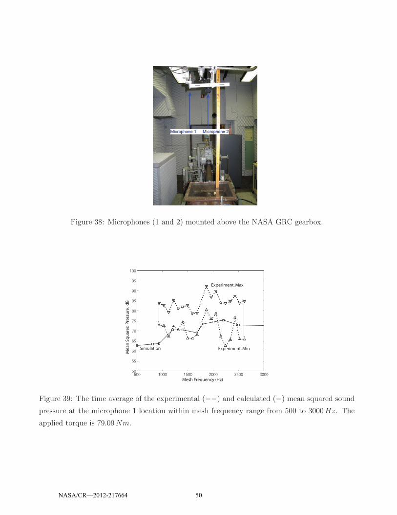
Figure 38: Microphones (1 and 2) mounted above the NASA GRC gearbox.

500 1000 1500 2000 2500 300050

55

60

65

70

75

80

85

90

95

100

Mesh Frequency (Hz)

Me

an

Sq

ua

red

Pre

ssu

re,

dB

Simulation Experiment, Min

Experiment, Max

Figure 39: The time average of the experimental (−−) and calculated (−) mean squared sound

pressure at the microphone 1 location within mesh frequency range from 500 to 3000Hz. The

applied torque is 79.09Nm.

NASA/CR—2012-217664 50

0 2000 4000 6000 8000 100000

0.02

0.04

0.06

0.08

0.1

0.12

0.14

0.16

0.18Measurement

Mesh Freq (Hz)

Sou

nd P

ress

ure,

Pa

0 2000 4000 6000 8000 100000

0.02

0.04

0.06

0.08

0.1

0.12

0.14

0.16

0.18Simulation

Mesh Freq (Hz)

Sou

nd P

ress

ure,

Pa

Figure 40: Frequency spectrum of the measured (left) and simulated (right) sound pressure at

the microphone 1 location when mesh frequency is 2000Hz. The applied torque is 79.09Nm.

6.4 Noise Radiation Properties with Different Bearings

This section investigates the effectiveness of fluid film wave bearings in reducing noise. To

that end, sound pressure and power of the radiated noise are compared between fluid film

wave and rolling element bearings.

Sound pressure at the microphone 1 location excited by the first (left) and second

(right) mesh frequency harmonics is compared between rolling element and wave bearings

in Figure 41. The sound pressure of wave bearings is generally higher than with rolling

element bearings. The difference is frequency dependent. When the second mesh frequency

harmonic is near 3803Hz (dominant mesh deflection mode), sound pressure with rolling

element bearings is similar in shape and amplitude to that with wave bearings. The noise

radiation is independent of bearing types at this frequency.

The sound power radiated from the gearbox is also compared between wave and rolling

element bearings in Figure 42. The sound power level of the gearbox with rolling element

and wave bearings is also speed-dependent. The radiated gearbox sound power with rolling

element bearings is lower than that with fluid film wave bearings in general within the speed

range of interest. There is no obvious benefit to replace rolling element bearings with wave

bearings to reduce the gearbox noise within the speed range of interest, given the two

dimensional wave bearing model used [38, 39].

NASA/CR—2012-217664 51

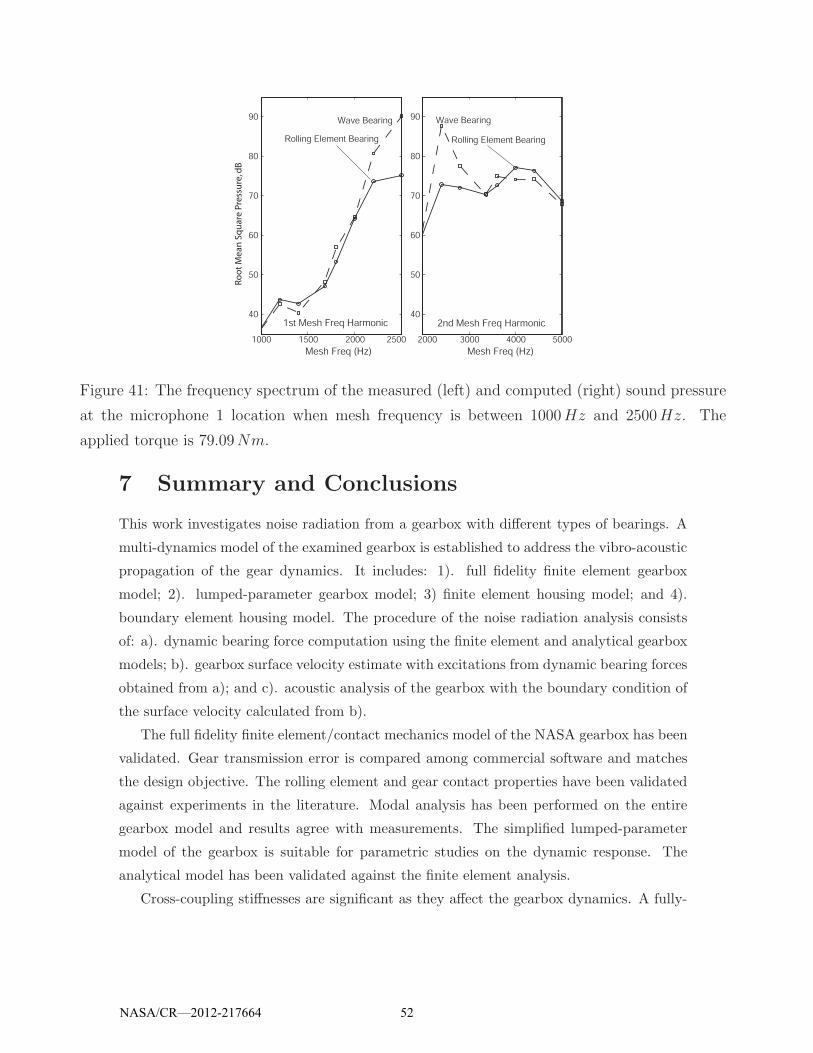
1000 1500 2000 2500

40

50

60

70

80

90

2000 3000 4000 5000

40

50

60

70

80

90

Ro

ot

Me

an

Sq

ua

re P

ress

ure

, dB

Mesh Freq (Hz) Mesh Freq (Hz)

Wave Bearing Wave Bearing

Rolling Element Bearing Rolling Element Bearing

1st Mesh Freq Harmonic 2nd Mesh Freq Harmonic

Figure 41: The frequency spectrum of the measured (left) and computed (right) sound pressure

at the microphone 1 location when mesh frequency is between 1000Hz and 2500Hz. The

applied torque is 79.09Nm.

7 Summary and Conclusions

This work investigates noise radiation from a gearbox with different types of bearings. A

multi-dynamics model of the examined gearbox is established to address the vibro-acoustic

propagation of the gear dynamics. It includes: 1). full fidelity finite element gearbox

model; 2). lumped-parameter gearbox model; 3) finite element housing model; and 4).

boundary element housing model. The procedure of the noise radiation analysis consists

of: a). dynamic bearing force computation using the finite element and analytical gearbox

models; b). gearbox surface velocity estimate with excitations from dynamic bearing forces

obtained from a); and c). acoustic analysis of the gearbox with the boundary condition of

the surface velocity calculated from b).

The full fidelity finite element/contact mechanics model of the NASA gearbox has been

validated. Gear transmission error is compared among commercial software and matches

the design objective. The rolling element and gear contact properties have been validated

against experiments in the literature. Modal analysis has been performed on the entire

gearbox model and results agree with measurements. The simplified lumped-parameter

model of the gearbox is suitable for parametric studies on the dynamic response. The

analytical model has been validated against the finite element analysis.

Cross-coupling stiffnesses are significant as they affect the gearbox dynamics. A fully-

NASA/CR—2012-217664 52

40

50

60

70

80

40

50

60

70

80

30

40

50

60

70

80

0

20

40

60

80

0

20

40

60

80

0

20

40

60

80

1st Harmonic 2nd Harmonic 3rd Harmonic

4th Harmonic 5th Harmonic 6th Harmonic

So

un

d P

ow

er

(dB

)

0.5 1.0 1.5 2.0 2.50.5 1.0 1.5 2.0 2.5 0.5 1.0 1.5 2.0 2.5

0.5 1.0 1.5 2.0 2.5 0.5 1.0 1.5 2.0 2.5 0.5 1.0 1.5 2.0 2.5

Mesh Frequency, kHz

Figure 42: Sound power of radiated gearbox noise excited by certain mesh frequency harmonics

of bearing forces with rolling element (−) and fluid film wave bearings (−−) at 79.09Nm input

torque. The excitation from 1st to 6th mesh frequency harmonics of bearing forces are considered

during the computation. A weighing filter (ISO standard) is used to adjust sound pressure levels.

populated stiffness matrix is needed to fully represent rolling element bearings. Bearing

stiffnesses fluctuate periodically as rolling elements enter and leave the region of loaded

rollers. These stiffness variations could excite gearbox vibration.

This acoustic model has been validated by comparing against theoretical solutions and

measurements taken at the NASA GRC gearbox. The transfer function method determines

sound pressure and power for arbitrary bearings, which is exceptionally suitable for the

gearbox optimization study to reduce noise. Noise radiation property of fluid film wave

bearings is speed-dependent, and wave bearings are not superior to rolling element bearing

in reducing gearbox noise. An one-way vibro-acoustic pass of the gearbox is present at the

mesh deflection mode. Gear dynamics significantly affects the housing vibration and noise

radiation. Housing and bearings, however, have limited effects on the gear vibration.

NASA/CR—2012-217664 53

References

[1] Harris, T. A., 1990. Rolling bearing analysis, 3rd ed. John Wiley and Sons, Inc.

[2] Gargiulo, Jr., E. P., 1980. “A simple way to estimate bearing stiffness”. Mechine

Design, pp. 107–110.

[3] While, M. F., 1979. “Rolling element bearing vibration transfer characteristics: Effect

of stiffness”. Journal of Applied Mechanics, 46, pp. 677–684.

[4] Royston, T. J., and Basdogan, I., 1998. “Vibration transmission through self-aligning

(spherical) rolling element bearings: Theory and experiment”. Journal of Sound and

Vibration, 215(5), pp. 997–1014.

[5] Kraus, J., Blech, J. J., and Braun, S. G., 1987. “In situ determination of rolling

bearing stiffness and damping by modal analysis”. Journal of Vibration, Acoustics,

Stress, and Reliability in Design, 109, pp. 235–240.

[6] Seybert, A. F., Wu, T. W., and Atherton, W., 1992. “Comparison of analysis and

experiment for gearbox noise”. NASA Technical Memorandum 251523. National

Aeronautic and Space Administration, Cleveland Lewis Reseach Center.

[7] Eritenel, T., and Parker, R. G., 2011. “An investigation of tooth mesh nonlinearity

and partial contact loss in gear pairs using a lumped-parameter model”. Mechanism

and Machine Theory. Submitted.

[8] Kahraman, A., and Blankenship, G. W., 1999. “Effect of involute tip relief on dynamic

response of spur gear pairs”. Journal of Mechanical Design, 121(1), Mar., pp. 112–

118.

[9] Mucchi, E., and Vecchio, A., 2010. “Acoustical signature analysis of a helicopter cabin

in steady-state and run up operational conditions”. Measurement, 43, p. 283293.

[10] Hoffmann, F., Maier, R., Janker, P., Hermle, F., and Berthe, A., 2006. “Helicopter

interior noise reduction by using active gearbox structs”. in: Proceedings of the 12th

AIAA/CEAS Aerospace Conference, May. Massachusetts, Cambridge.

[11] Dozio, L., Corbetta, W., Vigono, E., Forghieri, A., Ghiringhelli, G., and Cenedese,

F., 2006. “Active solutions for the reduction of the transmission of structure-borne

noise to the cabin structure on a a109 mockup”. Proceedings of ISMA, September.

Leuven, Belgium.

NASA/CR—2012-217664 54

[12] Viswamurthy, S., and Ganguli, R., 2004. “An optimization approach to vibration

reduction in helicopter rotors with multiple active trailing edge flaps,”. Aerospace

Science and Technology, 8(3), p. 185194.

[13] Hirsch, S., Jayachandran, V., and Sun, J. Q., Composite Structures. “Structural-

acoustic control for quieter aircraft interior-smart trim technology”. 1998, 42(2),

p. 189202.

[14] Randall, R., 2004. “Detection and diagnosis of incipient bearing failure in helicopter

gearboxes”. Engineering Failure Analysis II, p. 177 190.

[15] He, S., Singh, R., and Pavic, G., 2008. “Effect of sliding friction on gear noise based on

a refined vibro-acoustic formulation”. Journal of Noise Control Engineering, 56(3),

pp. 164–175.

[16] Lim, T. C., and Singh, R., 1991. “Statistical energy analysis of a gearbox with

emphasis on the bearing path”. Journal of Noise Control Engineering, 37(2), pp. 63–

69.

[17] Lim, T. C., and Singh, R., 1989. “A review of gear housing dynamics and acoustic

literature”. NASA Contractor Report 185148.

[18] Vijayakar, S. M. Calyx User’s Manual. Advanced Numerical Solutions LLC, Hilliard,

Ohio, 43026 USA. http://www.ansol.us/Manuals/Helical3DManual.pdf.

[19] http://www.ansol.us/Products/Coustyx.

[20] Dimofte, F., 1995. “Wave journal bearing with compressible lubricant; part i: The

wave bearing concept and a comparison to the plain circular bearing”. STLE Tribology

Transaction, 38(1), p. 153160.

[21] Dimofte, F., and Addy, Jr., H. E., 1994. “Preliminary experimental results of a

three wave journal air bearing”. Proceedings of Advanced Earth-to-Orbit Propulsion

Technology Conference, 11, May, p. 375384.

[22] Dimofte, F., Proctor, M. P., Fleming, D. P., and Keith, Jr, T. G., 2000. “Wave

fluid film bearing tests for an aviation gearbox”. NASA Techanical Report,

NASA/TM2000-209766, Jan.

[23] Dimofte, F., 1995. “Wave journal bearing; part i: Analysis”. NASA Contractor Report

195431.

[24] Hambric, S. A., Hanford, A. D., Shepherd, M. R., Campbell, R. L., and Smith, E. C.,

2010. “Rotorcraft transmission noise path model, including distributed fluid film

bearing impedance modeling”. NASA Technical Report. Contract No. NNC08CB07C.

NASA/CR—2012-217664 55

[25] Parker, R. G., Agashe, V., and Vijayakar, S. M., 2000. “Dynamic response of a

planetary gear system using a finite element/contact mechanics model”. Journal of

Mechanical Design, 122(3), Sept., pp. 304–310.

[26] Parker, R. G., Vijayakar, S. M., and Imajo, T., 2000. “Non-linear dynamic response

of a spur gear pair: Modelling and experimental comparisons”. Journal of Sound and

Vibration, 237(3), Oct., pp. 435–455.

[27] Ambarisha, V. K., and Parker, R. G., 2007. “Nonlinear dynamics of planetary gears

using analytical and finite element models”. Journal of Sound and Vibration, 302,

pp. 577–595.

[28] Bahk, C.-J., and Parker, R., 2011. “Analytical solution for the nonlinear dynamics of

planetary gears”. ASME Journal of Computational and Nonlinear Dynamics, 6(2),

p. 021007.

[29] Liu, G., and Parker, R. G., 2008. “Dynamic modeling and analysis of tooth pro-

file modification of multi-mesh gears”. ASME Journal of Mechanical Design, 130,

pp. 121402–1.

[30] Liu, G., and Parker, R. G., 2008. “Impact of tooth friction and its bending effect on

gear dynamics”. Journal of Sound and Vibration, 320(4-5), Mar., pp. 1039–1063.

[31] Guo, Y., and Parker, R. G., 2010. “Stiffness matrix calculation of rolling element

bearings using a finite element/contact mechanics model”. Mechanism and Machine

Theory. Submitted.

[32] Gunda, R., 2008. “Boundary element acoustics and the fast multipole method (fmm)”.

Sound and Vibration, March.

[33] Oswald, F. B., Townsend, D. P., Valco, M. J., Spencer, R. H., Drago, R. J., and

Lenski, J. W., 1994. Influence of gear design parameters on gearbox radiated noise.

Tech. Rep. ARL TR-381, NASA.

[34] Greogory, R. W., Harris, S. L., and Munro, R. G., 1963. “Dynamic behavior of spur

gears”. Proceedings of the institution of mechanical engineers, 178, pp. 261–266.

[35] Vijayakar, S. M., 1991. “A combined surface integral and finite element solution for

a three-dimensional contact problem”. International Journal for Numerical Methods

in Engineering, 31, pp. 524–546.

[36] Liu, G., and Parker, R., 2008. “Nonlinear dynamics of idler gearsets”. Nonlinear

Dynamics, 53, pp. 345–367.

NASA/CR—2012-217664 56

[37] Guo, Y., and Parker, R. G., 2011. “Dynamic analysis of planetary gears with bearing

clearance”. ASME Journal of Computational and Nonlinear Dynamics. Submitted.

[38] Hanford, A., 2009. Wave Journal Bearing Dynamic Coefficients Users Manual.

ARL/Penn State.

[39] Campbell, R. L. a., 2003. “Distributed journal bearing dynamic coefficients for struc-

tural finite element models”. Proceedings of ASME IMECE. NCA-43770.

[40] Jones, A. B., 1946. “Analysis of stresses and deflections”. New Departure Engineering

Data. General Motors.

[41] Palmgren, A., 1959. Ball and roller bearing engineering. S. H. Burbank, Philadelphia,.

[42] Brandlein, J., Eschmann, P., Hasbargen, L., and Weigand, K., 1999. Ball and roller

bearings: theory, design and application. John Wiley and Sons.

[43] Oswald, F. B., Lin, H. H., and Delgado, I. R., 1996. “Dynamic analysis of spur gear

transmissions (danst)”. NASA Technical Memorandum 107291. Technical Report

ARLTR1189.

[44] Guo, Y., Parker, R. G., Eritenel, T., and Ericson, T. M., 2011. Vibration propagation

of gear dynamics in a gear-bearing-housing system using mathematical modeling and

finite element analysis. Tech. rep., NASA Contract NNC08CB03C.

[45] Blankenship, G. W., and Singh, R., 1995. “Dynamic force transmissibility in helical

gear pairs”. Mechanism and Machine Theory, 30(3), Apr., pp. 323–339.

[46] Blankenship, G. W., and Singh, R., 1995. “A new gear mesh interface dynamic model

to predict multi dimensional force coupling and excitation”. Mechanism and Machine

Theory, 30(1), Jan., pp. 43–57.

[47] Salzer, M., Smith, J., and Welbourn, D., 1977. “Simulation of noise from gears when

varying design and manufacturing parameters”. Proceedings of the World Congress

on Gearing, 1, pp. 297–308.

[48] Kahraman, A., 1993. “Effect of axial vibrations on the dynamics of a helical gear

pair”. Journal of Vibration and Acoustics, 115(1), Jan., pp. 33–39.

[49] Andersson, A., and Vedmar, L., 2003. “A dynamic model to determine vibrations in

involute helical gears”. Journal of Sound and Vibration, 260(2), Feb., pp. 195–212.

[50] Velex, P., and Maatar, M., 1996. “A mathematical model for analyzing the influence

of shape deviations and mounting errors on gear dynamic behavior”. Journal of Sound

and Vibration, 191(5), Apr., pp. 629–660.

NASA/CR—2012-217664 57

[51] He, S., Gunda, R., and Singh, R., 2007. “Inclusion of sliding friction in contact

dynamics model for helical gears”. Journal of Mechanical Design, 129, Jan., pp. 48–

57.

[52] Conry, T. F., and Seireg, A., 1973. “Mathematical programming technique for eval-

uation of load distribution and optimal modification for gear systems”. Journal of

Engineering for Industry, 95(4), pp. 1115–1122.

[53] Ogawa, Y., Matsumura, S., Houjoh, H., Sato, T., and Umezawa, K., 2000. “Rota-

tional vibration of a spur gear pair considering tooth helix deviation: Development of

simulator and verification”. JSME International Journal, Series C, 43(2), pp. 423–

431.

[54] Kinsler, L. E., Frey, A. R., Coppens, A. B., and Sanders, J. V., 1982. Fundamentals

of Acoustics. Wiley, New York.

NASA/CR—2012-217664 58

REPORT DOCUMENTATION PAGE Form Approved OMB No. 0704-0188

The public reporting burden for this collection of information is estimated to average 1 hour per response, including the time for reviewing instructions, searching existing data sources, gathering and maintaining the data needed, and completing and reviewing the collection of information. Send comments regarding this burden estimate or any other aspect of this collection of information, including suggestions for reducing this burden, to Department of Defense, Washington Headquarters Services, Directorate for Information Operations and Reports (0704-0188), 1215 Jefferson Davis Highway, Suite 1204, Arlington, VA 22202-4302. Respondents should be aware that notwithstanding any other provision of law, no person shall be subject to any penalty for failing to comply with a collection of information if it does not display a currently valid OMB control number. PLEASE DO NOT RETURN YOUR FORM TO THE ABOVE ADDRESS. 1. REPORT DATE (DD-MM-YYYY) 01-08-2012

2. REPORT TYPE Final Contractor Report

3. DATES COVERED (From - To)

4. TITLE AND SUBTITLE Vibration Propagation of Gear Dynamics in a Gear-Bearing Housing System Using Mathematical Modeling and Finite Element Analysis

5a. CONTRACT NUMBER NNC08CB03C

5b. GRANT NUMBER

5c. PROGRAM ELEMENT NUMBER

6. AUTHOR(S) Parker, Robert, G.; Guo, Yi; Eritenel, Tugan; Ericson, Tristan, M.

5d. PROJECT NUMBER

5e. TASK NUMBER

5f. WORK UNIT NUMBER WBS 877868.02.07.03.04.01

7. PERFORMING ORGANIZATION NAME(S) AND ADDRESS(ES) The Ohio State University

8. PERFORMING ORGANIZATION REPORT NUMBER E-18341

9. SPONSORING/MONITORING AGENCY NAME(S) AND ADDRESS(ES) National Aeronautics and Space Administration Washington, DC 20546-0001

10. SPONSORING/MONITOR'S ACRONYM(S) NASA

11. SPONSORING/MONITORING REPORT NUMBER NASA/CR-2012-217664

12. DISTRIBUTION/AVAILABILITY STATEMENT Unclassified-Unlimited Subject Category: 37 Available electronically at http://www.sti.nasa.gov This publication is available from the NASA Center for AeroSpace Information, 443-757-5802

13. SUPPLEMENTARY NOTES

14. ABSTRACT Vibration and noise caused by gear dynamics at the meshing teeth propagate through power transmission components to the surrounding environment. This study is devoted to developing computational tools to investigate the vibro-acoustic propagation of gear dynamics through a gearbox using different bearings. Detailed finite element/contact mechanics and boundary element models of the gear/bearing/housing system are established to compute the system vibration and noise propagation. Both vibration and acoustic models are validated by experiments including the vibration modal testing and sound field measurements. The effectiveness of each bearing type to disrupt vibration propagation is speed-dependent. Housing plays an important role in noise radiation .It, however, has limited effects on gear dynamics. Bearings are critical components in drivetrains. Accurate modeling of rolling element bearings is essential to assess vibration and noise of drivetrain systems. This study also seeks to fully describe the vibro-acoustic propagation of gear dynamics through a power-transmission system using rolling element and fluid film wave bearings. Fluid film wave bearings, which have higher damping than rolling element bearings, could offer an energy dissipation mechanism that reduces the gearbox noise. The effectiveness of each bearing type to disrupt vibration propagation in explored using multi-body computational models. These models include gears, shafts, rolling element and fluid film wave bearings, and the housing. Radiated noise is mapped from the gearbox surface to surrounding environment. The effectiveness of rolling element and fluid film wave bearings in breaking the vibro-acoustic propagation path from the gear to the housing is investigated. 15. SUBJECT TERMS Gear noise; Noise transmission; Vibration; Bearings; Rolling element bearings; Journal bearings; Wave journal bearings

16. SECURITY CLASSIFICATION OF: 17. LIMITATION OF ABSTRACT UU

18. NUMBER OF PAGES

64

19a. NAME OF RESPONSIBLE PERSON STI Help Desk (email:help@sti.nasa.gov)

a. REPORT U

b. ABSTRACT U

c. THIS PAGE U

19b. TELEPHONE NUMBER (include area code) 443-757-5802

Standard Form 298 (Rev. 8-98)Prescribed by ANSI Std. Z39-18