Embed Size (px)
Citation preview
Chapter 2Vibration Dynamics
In this chapter, we review the dynamics of vibrations and the methods of deriv-ing the equations of motion of vibrating systems. The Newton–Euler and Lagrangemethods are the most common methods of deriving the equations of motion. Havingsymmetric coefficient matrices is the main advantage of using the Lagrange methodin mechanical vibrations.
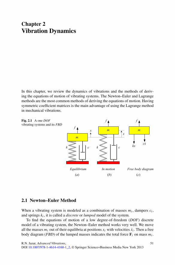
Fig. 2.1 A one DOFvibrating systems and its FBD
2.1 Newton–Euler Method
When a vibrating system is modeled as a combination of masses mi , dampers ci ,and springs ki , it is called a discrete or lumped model of the system.
To find the equations of motion of a low degree-of-freedom (DOF) discretemodel of a vibrating system, the Newton–Euler method works very well. We moveall the masses mi out of their equilibria at positions xi with velocities xi . Then a freebody diagram (FBD) of the lumped masses indicates the total force Fi on mass mi .
R.N. Jazar, Advanced Vibrations,DOI 10.1007/978-1-4614-4160-1_2, © Springer Science+Business Media New York 2013
51
52 2 Vibration Dynamics
Employing the momentum pi = mi vi of the mass mi , the Newton equation providesus with the equation of motion of the system:
Fi = d
dtpi = d
dt(mi vi ) (2.1)
When the motion of a massive body with mass moment Ii is rotational, then its equa-tion of motion will be found by Euler equation, in which we employ the moment ofmomentum Li = Ii ω of the mass mi :
Mi = d
dtLi = d
dt(Ii ω) (2.2)
For example, Fig. 2.1 illustrates a one degree-of-freedom (DOF) vibrating sys-tem. Figure 2.1(b) depicts the system when m is out of the equilibrium position at x
and moving with velocity x, both in positive direction. The FBD of the system is asshown in Fig. 2.1(c). The Newton equation generates the equations of motion:
ma = −cv − kx + f (x, v, t) (2.3)
The equilibrium position of a vibrating system is where the potential energy ofthe system, V , is extremum:
∂V
∂x= 0 (2.4)
We usually set V = 0 at the equilibrium position. Linear systems with constantstiffness have only one equilibrium or infinity equilibria, while nonlinear systemsmay have multiple equilibria. An equilibrium is stable if
∂2V
∂x2> 0 (2.5)
and is unstable if
∂2V
∂x2< 0 (2.6)
The geometric arrangement and the number of employed mechanical elementscan be used to classify discrete vibrating systems. The number of masses times theDOF of each mass makes the total DOF of the vibrating system n. Each indepen-dent DOF of a mass is indicated by an independent variable, called the generalizedcoordinate. The final set of equations would be n second-order differential equa-tions to be solved for n generalized coordinates. When each moving mass has oneDOF, then the system’s DOF is equal to the number of masses. The DOF mayalso be defined as the minimum number of independent coordinates that defines theconfiguration of a system.
The equation of motion of an n DOF linear mechanical vibrating system of canalways be arranged as a set of second-order differential equations
[m]x + [c]x + [k]x = F (2.7)
2.1 Newton–Euler Method 53
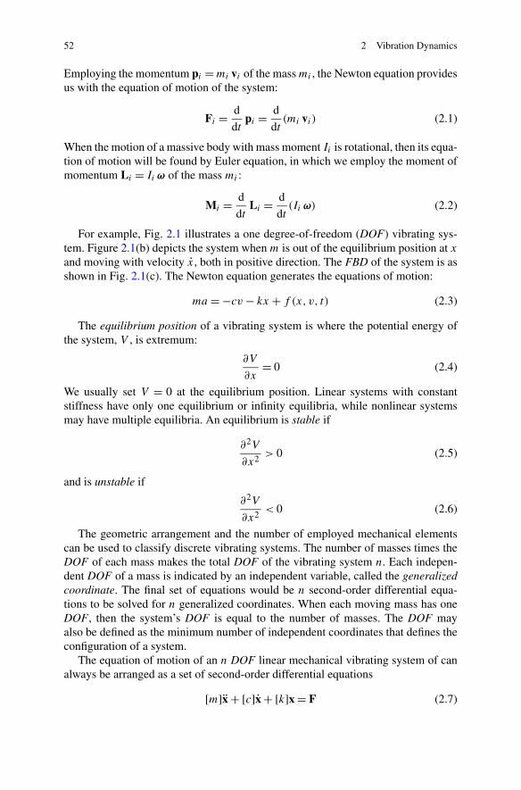
Fig. 2.2 Two, three, and oneDOF models for verticalvibrations of vehicles
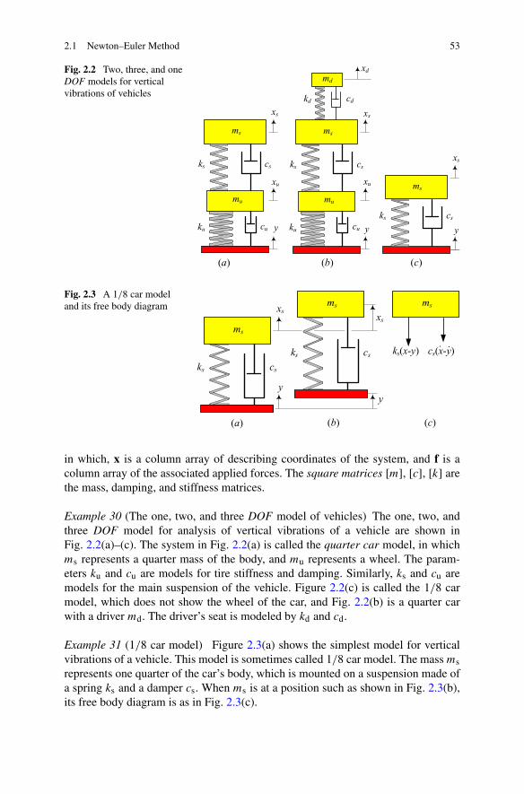
Fig. 2.3 A 1/8 car modeland its free body diagram
in which, x is a column array of describing coordinates of the system, and f is acolumn array of the associated applied forces. The square matrices [m], [c], [k] arethe mass, damping, and stiffness matrices.
Example 30 (The one, two, and three DOF model of vehicles) The one, two, andthree DOF model for analysis of vertical vibrations of a vehicle are shown inFig. 2.2(a)–(c). The system in Fig. 2.2(a) is called the quarter car model, in whichms represents a quarter mass of the body, and mu represents a wheel. The param-eters ku and cu are models for tire stiffness and damping. Similarly, ks and cu aremodels for the main suspension of the vehicle. Figure 2.2(c) is called the 1/8 carmodel, which does not show the wheel of the car, and Fig. 2.2(b) is a quarter carwith a driver md. The driver’s seat is modeled by kd and cd.
Example 31 (1/8 car model) Figure 2.3(a) shows the simplest model for verticalvibrations of a vehicle. This model is sometimes called 1/8 car model. The mass msrepresents one quarter of the car’s body, which is mounted on a suspension made ofa spring ks and a damper cs. When ms is at a position such as shown in Fig. 2.3(b),its free body diagram is as in Fig. 2.3(c).

54 2 Vibration Dynamics
Fig. 2.4 Equivalentmass–spring vibrator for apendulum
Applying Newton’s method, the equation of motion would be
msx = −ks(xs − y) − cs(xs − y) (2.8)
which can be simplified to
msx + csxs + ksxs = ksy + csy (2.9)
The coordinate y indicates the input from the road and x indicates the absolutedisplacement of the body. Absolute displacement refers to displacement with respectto the motionless background.
Example 32 (Equivalent mass and spring) Figure 2.4(a) illustrates a pendulum madeby a point mass m attached to a massless bar with length l. The coordinate θ showsthe angular position of the bar. The equation of motion for the pendulum can befound by using the Euler equation and employing the FBD shown in Fig. 2.4(b):
IAθ =∑
MA (2.10)
ml2θ = −mgl sin θ (2.11)
Simplifying the equation of motion and assuming a very small swing angle yields
lθ + gθ = 0 (2.12)
This equation is equivalent to an equation of motion of a mass–spring system madeby a mass me ≡ l, and a spring with stiffness ke ≡ g. The displacement of the masswould be xe ≡ θ . Figure 2.4(c) depicts such an equivalent mass–spring system.
Example 33 (Gravitational force in rectilinear vibrations) When the direction ofthe gravitational force on a mass m is not varied with respect to the direction of
2.1 Newton–Euler Method 55
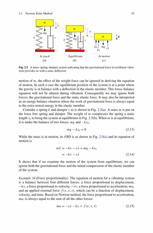
Fig. 2.5 A mass–spring–damper system indicating that the gravitational force in rectilinear vibra-tions provides us with a static deflection
motion of m, the effect of the weight force can be ignored in deriving the equationof motion. In such a case the equilibrium position of the system is at a point wherethe gravity is in balance with a deflection in the elastic member. This force–balanceequation will not be altered during vibration. Consequently we may ignore bothforces; the gravitational force and the static elastic force. It may also be interpretedas an energy balance situation where the work of gravitational force is always equalto the extra stored energy in the elastic member.
Consider a spring k and damper c as is shown in Fig. 2.5(a). A mass m is put onthe force free spring and damper. The weight of m compresses the spring a staticlength xs to bring the system at equilibrium in Fig. 2.5(b). When m is at equilibrium,it is under the balance of two forces, mg and −kxs:
mg − kxs = 0 (2.13)
While the mass is in motion, its FBD is as shown in Fig. 2.5(c) and its equation ofmotion is
mx = −kx − cx + mg − kxs
= −kx − cx (2.14)
It shows that if we examine the motion of the system from equilibrium, we canignore both the gravitational force and the initial compression of the elastic memberof the system.
Example 34 (Force proportionality) The equation of motion for a vibrating systemis a balance between four different forces: a force proportional to displacement,−kx, a force proportional to velocity, −cv, a force proportional to acceleration, ma,and an applied external force f (x, v, t), which can be a function of displacement,velocity, and time. Based on Newton method, the force proportional to acceleration,ma, is always equal to the sum of all the other forces:
ma = −cv − kx + f (x, v, t) (2.15)
56 2 Vibration Dynamics
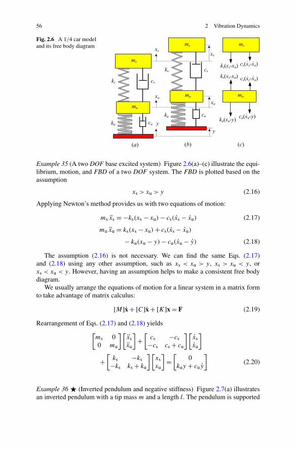
Fig. 2.6 A 1/4 car modeland its free body diagram
Example 35 (A two DOF base excited system) Figure 2.6(a)–(c) illustrate the equi-librium, motion, and FBD of a two DOF system. The FBD is plotted based on theassumption
xs > xu > y (2.16)
Applying Newton’s method provides us with two equations of motion:
ms xs = −ks(xs − xu) − cs(xs − xu) (2.17)
mu xu = ks(xs − xu) + cs(xs − xu)
− ku(xu − y) − cu(xu − y) (2.18)
The assumption (2.16) is not necessary. We can find the same Eqs. (2.17)and (2.18) using any other assumption, such as xs < xu > y, xs > xu < y, orxs < xu < y. However, having an assumption helps to make a consistent free bodydiagram.
We usually arrange the equations of motion for a linear system in a matrix formto take advantage of matrix calculus:
[M]x + [C]x + [K]x = F (2.19)
Rearrangement of Eqs. (2.17) and (2.18) yields[ms 00 mu
][xsxu
]+
[cs −cs
−cs cs + cu
][xsxu
]
+[
ks −ks−ks ks + ku
][xsxu
]=
[0
kuy + cuy
](2.20)
Example 36 � (Inverted pendulum and negative stiffness) Figure 2.7(a) illustratesan inverted pendulum with a tip mass m and a length l. The pendulum is supported

2.1 Newton–Euler Method 57
Fig. 2.7 An invertedpendulum with a tip mass m
and two supportive springs
by two identical springs attached to point B at a distance a < l from the pivot A.A free body diagram of the pendulum is shown in Fig. 2.7(b). The equation ofmotion may be found by taking a moment about A:
∑MA = IAθ (2.21)
mg(l sin θ) − 2kaθ(a cos θ) = ml2θ (2.22)
To derive Eq. (2.22) we assumed that the springs are long enough to remain almoststraight when the pendulum oscillates. Rearrangement and assuming a very small θ
show that the nonlinear equation of motion (2.22) can be approximated by
ml2θ + (mgl − 2ka2)θ = 0 (2.23)
which is equivalent to a linear oscillator:
meθ + keθ = 0 (2.24)
with an equivalent mass me and equivalent stiffness ke:
me = ml2 ke = mgl − 2ka2 (2.25)
The potential energy of the inverted pendulum is
V = −mgl(1 − cos θ) + ka2θ2 (2.26)
which has a zero value at θ = 0. The potential energy V is approximately equal tothe following equation if θ is very small:
V ≈ −1
2mglθ2 + ka2θ2 (2.27)

58 2 Vibration Dynamics
because
cos θ ≈ 1 − 1
2θ2 + O
(θ4) (2.28)
To find the equilibrium positions of the system, we may solve the equation ∂V/∂θ =0 for any possible θ :
∂V
∂θ= −2mglθ + 2ka2θ = 0 (2.29)
The solution of the equation is
θ = 0 (2.30)
which shows that the upright vertical position is the only equilibrium of the invertedpendulum as long as θ is very small. However, if
mgl = ka2 (2.31)
then any θ around θ = 0 would be an equilibrium position and, hence, the invertedpendulum would have an infinity of equilibria.
The second derivative of the potential energy
∂2V
∂x2= −2mgl + 2ka2 (2.32)
indicates that the equilibrium position θ = 0 is stable if
ka2 > mgl (2.33)
A stable equilibrium pulls the system back if it deviates from the equilibrium, whilean unstable equilibrium repels the system. Vibration happens when the equilibriumis stable.
This example also indicates the fact that having a negative stiffness is possibleby geometric arrangement of mechanical components of a vibrating system.
Example 37 � (Force function in equation of motion) Qualitatively, force is what-ever changes the motion, and quantitatively, force is whatever is equal to mass timesacceleration. Mathematically, the equation of motion provides us with a vectorialsecond-order differential equation
mr = F(r, r, t) (2.34)
We assume that the force function may generally be a function of time t , position r,and velocity r. In other words, the Newton equation of motion is correct as long aswe can show that the force is only a function of r, r, t .
If there is a force that depends on the acceleration, jerk, or other variables thatcannot be reduced to r, r, t , the system is not Newtonian and we do not know theequation of motion, because
F(r, r, r,...r , . . . , t) �= mr (2.35)
2.2 Energy 59
In Newtonian mechanics, we assume that force can only be a function of r, r, t andnothing else. In real world, however, force may be a function of everything; however,we always ignore any other variables than r, r, t .
Because Eq. (2.34) is a linear equation for force F, it accepts the superpositionprinciple. When a mass m is affected by several forces F1, F2,F3, . . . , we maycalculate their summation vectorially
F = F1 + F2 + F3 + · · · (2.36)
and apply the resultant force on m. So, if a force F1 provides us with accelerationr1, and F2 provides us with r2,
mr1 = F1 mr2 = F2 (2.37)
then the resultant force F3 = F1 + F2 provides us with the acceleration r3 such that
r3 = r1 + r2 (2.38)
To see that the Newton equation of motion is not correct when the force is notonly a function of r, r, t , let us assume that a particle with mass m is under twoacceleration dependent forces F1(x) and F2(x) on x-axis:
mx1 = F1(x1) mx2 = F2(x2) (2.39)
The acceleration of m under the action of both forces would be x3
mx3 = F1(x3) + F2(x3) (2.40)
however, though we must have
x3 = x1 + x2 (2.41)
we do have
m(x1 + x2) = F1(x1 + x2) + F2(x1 + x2)
�= F1(x1) + F2(x2) (2.42)
2.2 � Energy
In Newtonian mechanics, the acting forces on a system of bodies can be dividedinto internal and external forces. Internal forces are acting between bodies of thesystem, and external forces are acting from outside of the system. External forcesand moments are called the load. The acting forces and moments on a body arecalled a force system. The resultant or total force F is the sum of all the externalforces acting on the body, and the resultant or total moment M is the sum of all
60 2 Vibration Dynamics
the moments of the external forces about a point, such as the origin of a coordinateframe:
F =∑
i
Fi M =∑
i
Mi (2.43)
The moment M of a force F, acting at a point P with position vector rP , about apoint Q at rQ is
MQ = (rP − rQ) × F (2.44)
and, therefore, the moment of F about the origin is
M = rP × F (2.45)
The moment of the force about a directional line l passing through the origin is
Ml = u · (rP × F) (2.46)
where u is a unit vector on l. The moment of a force may also be called torque ormoment.
The effect of a force system is equivalent to the effect of the resultant force andresultant moment of the force system. Any two force systems are equivalent if theirresultant forces and resultant moments are equal. If the resultant force of a forcesystem is zero, the resultant moment of the force system is independent of the originof the coordinate frame. Such a resultant moment is called a couple.
When a force system is reduced to a resultant FP and MP with respect to areference point P , we may change the reference point to another point Q and findthe new resultants as
FQ = FP (2.47)
MQ = MP + (rP − rQ) × FP = MP + QrP × FP (2.48)
The momentum of a moving rigid body is a vector quantity equal to the total massof the body times the translational velocity of the mass center of the body:
p = mv (2.49)
The momentum p is also called the translational momentum or linear momentum.Consider a rigid body with momentum p. The moment of momentum, L, about a
directional line l passing through the origin is
Ll = u · (rC × p) (2.50)
where u is a unit vector indicating the direction of the line, and rC is the positionvector of the mass center C. The moment of momentum about the origin is
L = rC × p (2.51)
The moment of momentum L is also called angular momentum.

2.2 Energy 61
Kinetic energy K of a moving body point P with mass m at a position GrP , andhaving a velocity GvP , in the global coordinate frame G is
K = 1
2mGvP · GvP = 1
2mGv2
P (2.52)
where G indicates the global coordinate frame in which the velocity vector vP isexpressed. The work done by the applied force GF on m in moving from point 1 topoint 2 on a path, indicated by a vector Gr, is
1W2 =∫ 2
1
GF · dGr (2.53)
However,∫ 2
1
GF · dGr = m
∫ 2
1
Gd
dt
Gv · Gv dt = 1
2m
∫ 2
1
d
dtv2 dt
= 1
2m(v2
2 − v21
) = K2 − K1 (2.54)
which shows that 1W2 is equal to the difference of the kinetic energy of terminaland initial points:
1W2 = K2 − K1 (2.55)
Equation (2.55) is called the principle of work and energy. If there is a scalar po-tential field function V = V (x, y, z) such that
F = −∇V = −dV
dr= −
(∂V
∂xı + ∂V
∂yj + ∂V
∂zk
)(2.56)
then the principle of work and energy (2.55) simplifies to the principle of conserva-tion of energy,
K1 + V1 = K2 + V2 (2.57)
The value of the potential field function V = V (x, y, z) is the potential energy ofthe system.
Proof Consider the spatial integral of Newton equation of motion∫ 2
1F · dr = m
∫ 2
1a · dr (2.58)
We can simplify the right-hand side of the integral (2.58) by the change of variable∫ r2
r1
F · dr = m
∫ r2
r1
a · dr = m
∫ t2
t1
dvdt
· v dt
= m
∫ v2
v1
v · dv = 1
2m(v2
2 − v21
)(2.59)
62 2 Vibration Dynamics
The kinetic energy of a point mass m that is at a position defined by Gr and havinga velocity Gv is defined by (2.52). Whenever the global coordinate frame G is theonly involved frame, we may drop the superscript G for simplicity. The work doneby the applied force GF on m in going from point r1 to r2 is defined by (2.53).Hence the spatial integral of equation of motion (2.58) reduces to the principle ofwork and energy (2.55):
1W2 = K2 − K1 (2.60)
which says that the work 1W2 done by the applied force GF on m during the dis-placement r2 − r1 is equal to the difference of the kinetic energy of m.
If the force F is the gradient of a potential function V ,
F = −∇V (2.61)
then F · dr in Eq. (2.58) is an exact differential and, hence,
∫ 2
1F · dr =
∫ 2
1dV = −(V2 − V1) (2.62)
E = K1 + V1 = K2 + V2 (2.63)
In this case the work done by the force is independent of the path of motion betweenr1 and r2 and depends only upon the value of the potential V at start and end pointsof the path. The function V is called the potential energy; Eq. (2.63) is called theprinciple of conservation of energy, and the force F = −∇V is called a potential, or aconservative force. The kinetic plus potential energy of the dynamic system is calledthe mechanical energy of the system and is denoted by E = K +V . The mechanicalenergy E is a constant of motion if all the applied forces are conservative.
A force F is conservative only if it is the gradient of a stationary scalar function.The components of a conservative force will only be functions of space coordinates:
F = Fx(x, y, z)ı + Fy(x, y, z)j + Fz(x, y, z)k (2.64)
�
Example 38 (Energy and equation of motion) Whenever there is no loss of energyin a mechanical vibrating system, the sum of kinetic and potential energies is aconstant of motion:
E = K + V = const (2.65)
A system with constant energy is called a conservative system. The time derivativeof a constant of motion must be zero at all time.
The mass–spring system of Fig. 2.10 is a conservative system with the total me-chanical energy of
E = 1
2mx2 + 1
2kx2 (2.66)

2.2 Energy 63
Fig. 2.8 A multi DOFconservative vibrating system
Having a zero rate of energy,
E = mxx + kxx = x(mx + kx) = 0 (2.67)
and knowing that x cannot be zero at all times provides us with the equation ofmotion:
mx + kx = 0 (2.68)
Example 39 � (Energy and multi DOF systems) We may use energy method anddetermine the equations of motion of multi DOF conservative systems. Considerthe system in Fig. 2.8 whose mechanical energy is
E = K + V = 1
2m1x
21 + 1
2m2x
22 + 1
2m3x
23
+ 1
2k1x
21 + 1
2k2(x1 − x2)
2 + 1
2k3(x2 − x3)
2 + 1
2k4x
23 (2.69)
To find the first equation of motion associated to x1, we assume x2 and x3 are con-stant and take the time directive:
E = m1x1x1 + k1x1x1 + k2(x1 − x2)x1 = 0 (2.70)
Because x1 cannot be zero at all times, the first equation of motion is
m1x1 + k1x1 + k2(x1 − x2) = 0 (2.71)
To find the second equation of motion associated to x2, we assume that x1 and x3are constant and we take a time directive of E
E = m2x2x2 − k2(x1 − x2)x2 + k3(x2 − x3)x2 = 0 (2.72)
which provides us with
m2x2 − k2(x1 − x2) + k3(x2 − x3) = 0 (2.73)
To find the second equation of motion associated to x2, we assume that x1 and x3are constant and we take the time directive of E
E = m3x3x3 − k3(x2 − x3)x3 + k4x3x3 = 0 (2.74)
64 2 Vibration Dynamics
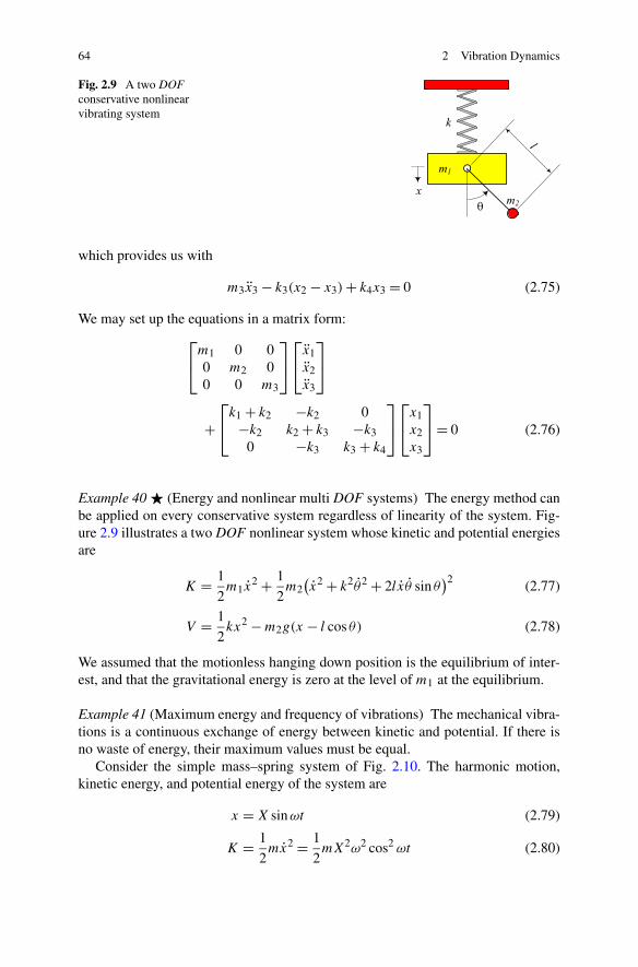
Fig. 2.9 A two DOFconservative nonlinearvibrating system
which provides us with
m3x3 − k3(x2 − x3) + k4x3 = 0 (2.75)
We may set up the equations in a matrix form:⎡
⎣m1 0 00 m2 00 0 m3
⎤
⎦
⎡
⎣x1x2x3
⎤
⎦
+⎡
⎣k1 + k2 −k2 0−k2 k2 + k3 −k3
0 −k3 k3 + k4
⎤
⎦
⎡
⎣x1x2x3
⎤
⎦ = 0 (2.76)
Example 40 � (Energy and nonlinear multi DOF systems) The energy method canbe applied on every conservative system regardless of linearity of the system. Fig-ure 2.9 illustrates a two DOF nonlinear system whose kinetic and potential energiesare
K = 1
2m1x
2 + 1
2m2
(x2 + k2θ2 + 2lxθ sin θ
)2 (2.77)
V = 1
2kx2 − m2g(x − l cos θ) (2.78)
We assumed that the motionless hanging down position is the equilibrium of inter-est, and that the gravitational energy is zero at the level of m1 at the equilibrium.
Example 41 (Maximum energy and frequency of vibrations) The mechanical vibra-tions is a continuous exchange of energy between kinetic and potential. If there isno waste of energy, their maximum values must be equal.
Consider the simple mass–spring system of Fig. 2.10. The harmonic motion,kinetic energy, and potential energy of the system are
x = X sinωt (2.79)
K = 1
2mx2 = 1
2mX2ω2 cos2 ωt (2.80)

2.2 Energy 65
Fig. 2.10 A mass–springsystem
Fig. 2.11 A wheel turning,without slip, over acylindrical hill
V = 1
2kx2 = 1
2kX2 sin2 ωt (2.81)
Equating the maximum K and V
1
2mX2ω2 = 1
2kX2 (2.82)
provides us with the frequency of vibrations:
ω2 = k
m(2.83)
Example 42 � (Falling wheel) Figure 2.11 illustrates a wheel turning, without slip,over a cylindrical hill. We may use the conservation of mechanical energy to findthe angle at which the wheel leaves the hill.
Initially, the wheel is at point A. We assume the initial kinetic and potential, andhence, the mechanical energies E = K + V are zero. When the wheel is turningover the hill, its angular velocity, ω, is
ω = v
r(2.84)
where v is the speed at the center of the wheel. At any other point B , the wheelachieves some kinetic energy and loses some potential energy. At a certain angle,where the normal component of the weight cannot provide more centripetal force,
mg cos θ = mv2
R + r(2.85)
66 2 Vibration Dynamics
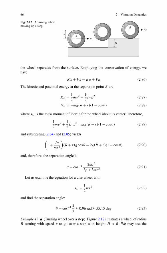
Fig. 2.12 A turning wheelmoving up a step
the wheel separates from the surface. Employing the conservation of energy, wehave
KA + VA = KB + VB (2.86)
The kinetic and potential energy at the separation point B are
KB = 1
2mv2 + 1
2ICω2 (2.87)
VB = −mg(R + r)(1 − cos θ) (2.88)
where IC is the mass moment of inertia for the wheel about its center. Therefore,
1
2mv2 + 1
2ICω2 = mg(R + r)(1 − cos θ) (2.89)
and substituting (2.84) and (2.85) yields
(1 + IC
mr2
)(R + r)g cos θ = 2g(R + r)(1 − cos θ) (2.90)
and, therefore, the separation angle is
θ = cos−1 2mr2
IC + 3mr2(2.91)
Let us examine the equation for a disc wheel with
IC = 1
2mr2 (2.92)
and find the separation angle:
θ = cos−1 4
7≈ 0.96 rad ≈ 55.15 deg (2.93)
Example 43 � (Turning wheel over a step) Figure 2.12 illustrates a wheel of radiusR turning with speed v to go over a step with height H < R. We may use the

2.2 Energy 67
principle of energy conservation and find the speed of the wheel after getting acrossthe step. Employing the conservation of energy, we have
KA + VA = KB + VB (2.94)
1
2mv2
1 + 1
2ICω2
1 + 0 = 1
2mv2
2 + 1
2ICω2
2 + mgH (2.95)
(m + IC
R2
)v2
1 =(
m + IC
R2
)v2
2 + 2mgH (2.96)
and, therefore,
v2 =√
v21 − 2gH
1 + IC
mR2
(2.97)
The condition for having a real v2 is
v1 >
√2gH
1 + IC
mR2
(2.98)
The second speed (2.97) and the condition (2.98) for a solid disc with IC = mR2/2are
v2 =√
v21 − 4
3Hg (2.99)
v1 >
√4
3Hg (2.100)
Example 44 (Newton equation) The application of a force system is emphasized byNewton’s second law of motion, which states that the global rate of change of linearmomentum is proportional to the global applied force:
GF =Gd
dt
Gp =Gd
dt
(mGv
)(2.101)
The second law of motion can be expanded to include rotational motions. Hence, thesecond law of motion also states that the global rate of change of angular momentumis proportional to the global applied moment:
GM =Gd
dt
GL (2.102)

68 2 Vibration Dynamics
Proof Differentiating the angular momentum (2.51) shows that
Gd
dt
GL =Gd
dt(rC × p) =
(GdrC
dt× p + rC ×
Gdpdt
)
= GrC ×Gdpdt
= GrC × GF = GM (2.103)
�
Example 45 � (Integral and constant of motion) Any equation of the form
f (q, q, t) = c (2.104)
c = f (q0, q0, t0) (2.105)
q = [q1 q2 · · · qn
](2.106)
with total differential
df
dt=
n∑
i=1
(∂f
∂qi
qi + ∂f
∂qi
qi
)+ ∂f
∂t= 0 (2.107)
that the generalized positions q and velocities q of a dynamic system must satisfyat all times t is called an integral of motion. The parameter c, of which the valuedepends on the initial conditions, is called a constant of motion. The maximumnumber of independent integrals of motion for a dynamic system with n degreesof freedom is 2n. A constant of motion is a quantity of which the value remainsconstant during the motion.
Any integral of motion is a result of a conservation principle or a combinationof them. There are only three conservation principles for a dynamic system: en-ergy, momentum, and moment of momentum. Every conservation principle is theresult of a symmetry in position and time. The conservation of energy indicates thehomogeneity of time, the conservation of momentum indicates the homogeneity inposition space, and the conservation of moment of momentum indicates the isotropyin position space.
Proof Consider a mechanical system with fC degrees of freedom. Mathematically,the dynamics of the system is expressed by a set of n = fC second-order differentialequations of n unknown generalized coordinates qi(t), i = 1,2, . . . , n:
qi = Fi(qi, qi , t) i = 1,2, . . . , n (2.108)
The general solution of the equations contains 2n constants of integrals.
qi = qi (c1, c2, . . . , cn, t) i = 1,2, . . . , n (2.109)
qi = qi(c1, c2, . . . , c2n, t) i = 1,2, . . . , n (2.110)
2.2 Energy 69
To determine these constants and uniquely identify the motion of the system, it isnecessary to know the initial conditions qi(t0), qi (t0), which specify the state of thesystem at some given instant t0:
cj = cj
(q(t0), q(t0), t0
)j = 1,2, . . . ,2n (2.111)
fj
(q(t), q(t), t
) = cj
(q(t0), q(t0), t0
)(2.112)
Each of these functions fj is an integral of the motion and each ci is a constant ofthe motion. An integral of motion may also be called a first integral, and a constantof motion may also be called a constant of integral.
When an integral of motion is given,
f1(q, q, t) = c1 (2.113)
we can substitute one of the equations of (2.108) with the first-order equation of
q1 = f (c1, qi, qi+1, t) i = 1,2, . . . , n (2.114)
and solve a set of n − 1 second-order and one first-order differential equations:{
qi+1 = Fi+1(qi, qi , t)
q1 = f (c1, qi, qi+1, t)i = 1,2, . . . , n (2.115)
If there exist 2n independent first integrals fj , j = 1,2, . . . ,2n, then instead of solv-ing n second-order equations of motion (2.108), we can solve a set of 2n algebraicequations
fj (q, q) = cj
(q(t0), q(t0), t0
)j = 1,2, . . . ,2n (2.116)
and determine the n generalized coordinates qi , i = 1,2, . . . , n:
qi = qi(c1, c2, . . . , c2n, t) i = 1,2, . . . , n (2.117)
Generally speaking, an integral of motion f is a function of generalized coordi-nates q and velocities q such that its value remains constant. The value of an integralof motion is the constant of motion c, which can be calculated by substituting thegiven value of the variables q(t0), q(t0) at the associated time t0. �
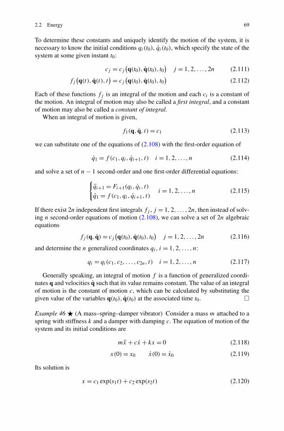
Example 46 � (A mass–spring–damper vibrator) Consider a mass m attached to aspring with stiffness k and a damper with damping c. The equation of motion of thesystem and its initial conditions are
mx + cx + kx = 0 (2.118)
x(0) = x0 x(0) = x0 (2.119)
Its solution is
x = c1 exp(s1t) + c2 exp(s2t) (2.120)

70 2 Vibration Dynamics
Fig. 2.13 A planar pendulum
s1 = c − √c2 − 4km
−2ms2 = c + √
c2 − 4km
−2m(2.121)
Taking the time derivative, we find x:
x = c1s1 exp(s1t) + c2s2 exp(s2t) (2.122)
Using x and x, we determine the integrals of motion f1 and f2:
f1 = x − xs2
(s1 − s2) exp(s1t)= c1 (2.123)
f2 = x − xs1
(s2 − s1) exp(s2t)= c2 (2.124)
Because the constants of integral remain constant during the motion, we can calcu-late their value at any particular time such as t = 0:
c1 = x0 − x0s2
(s1 − s2)c2 = x0 − x0s1
(s2 − s1)(2.125)
Substituting s1 and s2 provides us with the constants of motion c1 and c2:
c1 =√
c2 − 4km(cx0 + x0√
c2 − 4km + 2mx0)
2(c2 − 4km)(2.126)
c2 =√
c2 − 4km(cx0 − x0√
c2 − 4km + 2mx0)
2(c2 − 4km)(2.127)
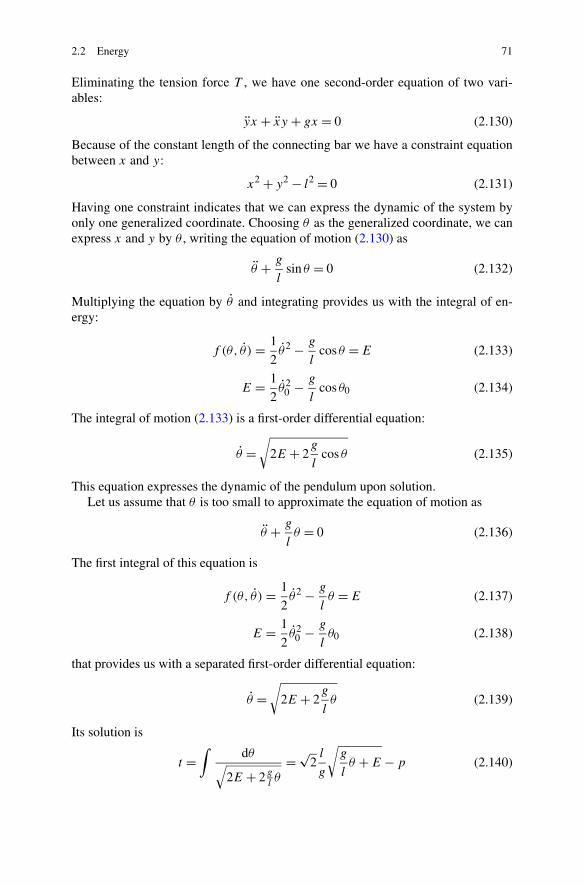
Example 47 � (Constraint and first integral of a pendulum) Figure 2.13(a) illus-trates a planar pendulum. The free body diagram of Fig. 2.13(b) provides us withtwo equations of motion:
mx = −Tx
l(2.128)
my = −mg + Ty
l(2.129)
2.2 Energy 71
Eliminating the tension force T , we have one second-order equation of two vari-ables:
yx + xy + gx = 0 (2.130)
Because of the constant length of the connecting bar we have a constraint equationbetween x and y:
x2 + y2 − l2 = 0 (2.131)
Having one constraint indicates that we can express the dynamic of the system byonly one generalized coordinate. Choosing θ as the generalized coordinate, we canexpress x and y by θ , writing the equation of motion (2.130) as
θ + g
lsin θ = 0 (2.132)
Multiplying the equation by θ and integrating provides us with the integral of en-ergy:
f (θ, θ) = 1
2θ2 − g
lcos θ = E (2.133)
E = 1
2θ2
0 − g
lcos θ0 (2.134)
The integral of motion (2.133) is a first-order differential equation:
θ =√
2E + 2g
lcos θ (2.135)
This equation expresses the dynamic of the pendulum upon solution.Let us assume that θ is too small to approximate the equation of motion as
θ + g
lθ = 0 (2.136)
The first integral of this equation is
f (θ, θ) = 1
2θ2 − g
lθ = E (2.137)
E = 1
2θ2
0 − g
lθ0 (2.138)
that provides us with a separated first-order differential equation:
θ =√
2E + 2g
lθ (2.139)
Its solution is
t =∫
dθ√2E + 2 g
lθ
= √2
l
g
√g
lθ + E − p (2.140)

72 2 Vibration Dynamics
where p is the second constant of motion:
p = l
gθ0 (2.141)
Now, let us ignore the energy integral and solve the second-order equation ofmotion (2.136):
θ = c1 cos
√g
lt + c2 sin
√g
lt (2.142)
The time derivative of the solution√
l
gθ = −c1 sin
√g
lt + c2 cos
√g
lt (2.143)
can be used to determine the integrals and constants of motion:
f1 = θ cos
√g
lt −
√l
gθ sin
√g
lt (2.144)
f2 = θ sin
√g
lt +
√l
gθ cos
√g
lt (2.145)
Using the initial conditions θ(0) = θ0, θ (0) = θ0, we have
c1 = θ0 c2 =√
l
gθ0 (2.146)
A second-order equation has only two constants of integrals. Therefore, we shouldbe able to express E and p in terms of c1 and c2 or vice versa:
E = 1
2θ2
0 − g
lθ0 = 1
2
g
lc2
2 − g
lc1 (2.147)
p = l
gθ0 = l
g
√g
lc2 (2.148)
c2 =√
l
gθ0 = g
l
√l
gp (2.149)
c1 = θ0 = 1
2
g
lp2 − l
gE (2.150)
E is the mechanical energy of the pendulum, and p is proportional to its moment ofmomentum.
2.3 Rigid Body Dynamics 73
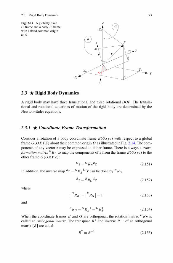
Fig. 2.14 A globally fixedG-frame and a body B-framewith a fixed common originat O
2.3 � Rigid Body Dynamics
A rigid body may have three translational and three rotational DOF. The transla-tional and rotational equations of motion of the rigid body are determined by theNewton–Euler equations.
2.3.1 � Coordinate Frame Transformation
Consider a rotation of a body coordinate frame B(Oxyz) with respect to a globalframe G(OXYZ) about their common origin O as illustrated in Fig. 2.14. The com-ponents of any vector r may be expressed in either frame. There is always a trans-formation matrix GRB to map the components of r from the frame B(Oxyz) to theother frame G(OXYZ):
Gr = GRBBr (2.151)
In addition, the inverse map Br = GR−1B
Gr can be done by BRG,
Br = BRGGr (2.152)
where∣∣GRB
∣∣ = ∣∣BRG
∣∣ = 1 (2.153)
andBRG = GR−1
B = GRTB (2.154)
When the coordinate frames B and G are orthogonal, the rotation matrix GRB iscalled an orthogonal matrix. The transpose RT and inverse R−1 of an orthogonalmatrix [R] are equal:
RT = R−1 (2.155)

74 2 Vibration Dynamics
Because of the matrix orthogonality condition, only three of the nine elements ofGRB are independent.
Proof Employing the orthogonality condition
r = (r · ı)ı + (r · j )j + (r · k)k (2.156)
and decomposition of the unit vectors of G(OXYZ) along the axes of B(Oxyz),
I = (I · ı)ı + (I · j )j + (I · k)k (2.157)
J = (J · ı)ı + (J · j )j + (J · k)k (2.158)
K = (K · ı)ı + (K · j )j + (K · k)k (2.159)
introduces the transformation matrix GRB to map the local axes to the global axes:
⎡
⎣I
J
K
⎤
⎦ =⎡
⎣I · ı I · j I · kJ · ı J · j J · kK · ı K · j K · k
⎤
⎦
⎡
⎣ı
j
k
⎤
⎦ = GRB
⎡
⎣ı
j
k
⎤
⎦ (2.160)
where
GRB =⎡
⎣I · ı I · j I · kJ · ı J · j J · kK · ı K · j K · k
⎤
⎦
=⎡
⎣cos(I , ı) cos(I , j ) cos(I , k)
cos(J , ı) cos(J , j ) cos(J , k)
cos(K, ı) cos(K, j ) cos(K, k)
⎤
⎦ (2.161)
Each column of GRB is the decomposition of a unit vector of the local frameB(Oxyz) in the global frame G(OXYZ):
GRB = [Gı Gj Gk
](2.162)
Similarly, each row of GRB is decomposition of a unit vector of the global frameG(OXYZ) in the local frame B(Oxyz).
GRB =⎡
⎣BIT
BJ T
BKT
⎤
⎦ (2.163)
so the elements of GRB are directional cosines of the axes of G(OXYZ) inB(Oxyz) or B in G. This set of nine directional cosines completely specifies theorientation of B(Oxyz) in G(OXYZ) and can be used to map the coordinates ofany point (x, y, z) to its corresponding coordinates (X,Y,Z).

2.3 Rigid Body Dynamics 75
Alternatively, using the method of unit-vector decomposition to develop the ma-trix BRG leads to
Br = BRGGr = GR−1
BGr (2.164)
BRG =⎡
⎣ı · I ı · J ı · Kj · I j · J j · Kk · I k · J k · K
⎤
⎦
=⎡
⎣cos(ı, I ) cos(ı, J ) cos(ı, K)
cos(j , I ) cos(j , J ) cos(j , K)
cos(k, I ) cos(k, J ) cos(k, K)
⎤
⎦ (2.165)
It shows that the inverse of a transformation matrix is equal to the transpose of thetransformation matrix,
GR−1B = GRT
B (2.166)
or
GRB · GRTB = I (2.167)
A matrix with condition (2.166) is called an orthogonal matrix. Orthogonality ofGRB comes from the fact that it maps an orthogonal coordinate frame to anotherorthogonal coordinate frame.
An orthogonal transformation matrix GRB has only three independent elements.The constraint equations among the elements of GRB will be found by applying thematrix orthogonality condition (2.166):
⎡
⎣r11 r12 r13r21 r22 r23r31 r32 r33
⎤
⎦
⎡
⎣r11 r21 r31r12 r22 r32r13 r23 r33
⎤
⎦ =⎡
⎣1 0 00 1 00 0 1
⎤
⎦ (2.168)
Therefore, the inner product of any two different rows of GRB is zero, and the innerproduct of any row of GRB by itself is unity:
r211 + r2
12 + r213 = 1
r221 + r2
22 + r223 = 1
r231 + r2
32 + r233 = 1
r11r21 + r12r22 + r13r23 = 0
r11r31 + r12r32 + r13r33 = 0
r21r31 + r22r32 + r23r33 = 0
(2.169)
76 2 Vibration Dynamics
These relations are also true for columns of GRB and evidently for rows andcolumns of BRG. The orthogonality condition can be summarized by the equation
3∑
i=1
rij rik = δjk j, k = 1,2,3 (2.170)
where rij is the element of row i and column j of the transformation matrix GRB
and δjk is the Kronecker delta δij ,
δij = δji ={
1 i = j
0 i �= j(2.171)
Equation (2.170) provides us with six independent relations that must be satisfiedby the nine directional cosines. Therefore, there are only three independent direc-tional cosines. The independent elements of the matrix GRB cannot be in the samerow or column or any diagonal.
The determinant of a transformation matrix is equal to unity,∣∣GRB
∣∣ = 1 (2.172)
because of Eq. (2.167) and noting that∣∣GRB · GRT
B
∣∣ = ∣∣GRB
∣∣ · ∣∣GRTB
∣∣ = ∣∣GRB
∣∣ · ∣∣GRB
∣∣ = ∣∣GRB
∣∣2 = 1 (2.173)
Using linear algebra and column vectors Gı,Gj , and Gk of GRB , we know that∣∣GRB
∣∣ = Gı · (Gj × Gk)
(2.174)
and because the coordinate system is right handed, we have Gj × Gk = Gı and,therefore,
∣∣GRB
∣∣ = GıT · Gı = +1 (2.175)
�
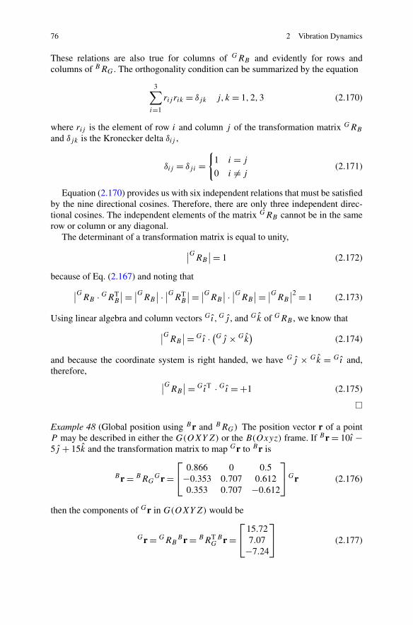
Example 48 (Global position using Br and BRG) The position vector r of a pointP may be described in either the G(OXYZ) or the B(Oxyz) frame. If Br = 10ı −5j + 15k and the transformation matrix to map Gr to Br is
Br = BRGGr =
⎡
⎣0.866 0 0.5
−0.353 0.707 0.6120.353 0.707 −0.612
⎤
⎦Gr (2.176)
then the components of Gr in G(OXYZ) would be
Gr = GRBBr = BRT
GBr =
⎡
⎣15.727.07
−7.24
⎤
⎦ (2.177)

2.3 Rigid Body Dynamics 77
Example 49 (Two-point transformation matrix) The global position vectors of twopoints P1 and P2, of a rigid body B are
GrP1 =⎡
⎣1.0771.3652.666
⎤
⎦ GrP2 =⎡
⎣−0.4732.239
−0.959
⎤
⎦ (2.178)
The origin of the body B(Oxyz) is fixed on the origin of G(OXYZ), and the pointsP1 and P2 are lying on the local x- and y-axis, respectively.
To find GRB , we use the local unit vectors Gı and Gj ,
Gı =GrP1
|GrP1 |=
⎡
⎣0.3380.4290.838
⎤
⎦ Gj =GrP2
|GrP2 |=
⎡
⎣−0.1910.902
−0.387
⎤
⎦ (2.179)
to obtain Gk:
Gk = ı × j =⎡
⎣−0.922−0.0290.387
⎤
⎦ (2.180)
Hence, the transformation matrix GRB would be
GRB = [Gı Gj Gk
] =⎡
⎣0.338 −0.191 −0.9220.429 0.902 −0.0290.838 −0.387 0.387
⎤
⎦ (2.181)
Example 50 (Length invariant of a position vector) Expressing a vector in differentframes utilizing rotation matrices does not affect the length and direction propertiesof the vector. Therefore, the length of a vector is an invariant property:
|r| = ∣∣Gr∣∣ = ∣∣Br
∣∣ (2.182)
The length invariant property can be shown as
|r|2 = GrTGr = [GRB
Br]TGRB
Br = BrTGRTB
GRBBr
= BrTBr (2.183)
Example 51 (Multiple rotation about global axes) Consider a globally fixed pointP at
Gr =⎡
⎣123
⎤
⎦ (2.184)
The body B will turn 45 deg about the X-axis and then 45 deg about the Y -axis.An observer in B will see P at
78 2 Vibration Dynamics
Br = Ry,−45 Rx,−45Gr
=⎡
⎣cos −π
4 0 − sin −π4
0 1 0sin −π
4 0 cos −π4
⎤
⎦
⎡
⎢⎣1 0 00 cos −π
4 sin −π4
0 − sin −π4 cos −π
4
⎤
⎥⎦
⎡
⎣123
⎤
⎦
=⎡
⎣0.707 0.5 0.5
0 0.707 −0.707−0.707 0.5 0.5
⎤
⎦
⎡
⎣123
⎤
⎦ =⎡
⎣3.207
−0.7071.793
⎤
⎦ (2.185)
To check this result, let us change the role of B and G. So, the body point at
Br =⎡
⎣123
⎤
⎦ (2.186)
undergoes an active rotation of 45 deg about the x-axis followed by 45 deg aboutthe y-axis. The global coordinates of the point would be
Br = Ry,45 Rx,45Gr (2.187)
soGr = [Ry,45 Rx,45]TBr = RT
x,45 RTy,45
Br (2.188)
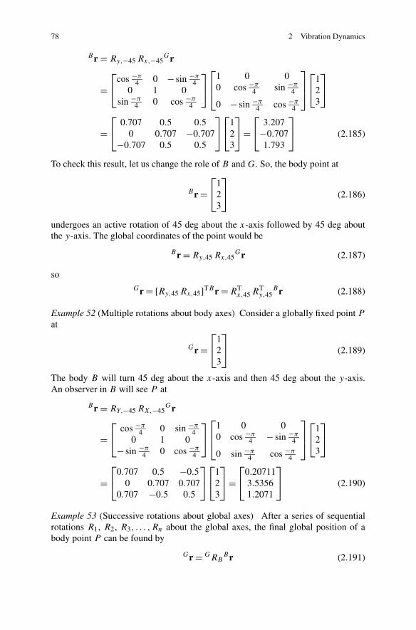
Example 52 (Multiple rotations about body axes) Consider a globally fixed point P
at
Gr =⎡
⎣123
⎤
⎦ (2.189)
The body B will turn 45 deg about the x-axis and then 45 deg about the y-axis.An observer in B will see P at
Br = RY,−45 RX,−45Gr
=⎡
⎣cos −π
4 0 sin −π4
0 1 0− sin −π
4 0 cos −π4
⎤
⎦
⎡
⎢⎣1 0 00 cos −π
4 − sin −π4
0 sin −π4 cos −π
4
⎤
⎥⎦
⎡
⎣123
⎤
⎦
=⎡
⎣0.707 0.5 −0.5
0 0.707 0.7070.707 −0.5 0.5
⎤
⎦
⎡
⎣123
⎤
⎦ =⎡
⎣0.207113.53561.2071
⎤
⎦ (2.190)
Example 53 (Successive rotations about global axes) After a series of sequentialrotations R1, R2, R3, . . . ,Rn about the global axes, the final global position of abody point P can be found by
Gr = GRBBr (2.191)
2.3 Rigid Body Dynamics 79
where
GRB = Rn · · ·R3 R2 R1 (2.192)
The vectors Gr and Br indicate the position vectors of the point P in the global andlocal coordinate frames, respectively. The matrix GRB , which transforms the localcoordinates to their corresponding global coordinates, is called the global rotationmatrix.
Because matrix multiplications do not commute, the sequence of performing ro-tations is important and indicates the order of rotations.
Proof Consider a body frame B that undergoes two sequential rotations R1 andR2 about the global axes. Assume that the body coordinate frame B is initiallycoincident with the global coordinate frame G. The rigid body rotates about a globalaxis, and the global rotation matrix R1 gives us the new global coordinate Gr1 ofthe body point:
Gr1 = R1Br (2.193)
Before the second rotation, the situation is similar to the one before the first rota-tion. We put the B-frame aside and assume that a new body coordinate frame B1
is coincident with the global frame. Therefore, the new body coordinate would beB1r ≡ Gr1. The second global rotation matrix R2 provides us with the new globalposition Gr2 of the body points B1r:
B1r = R2B1r (2.194)
Substituting (2.193) into (2.194) shows that
Gr = R2 R1Br (2.195)
Following the same procedure we can determine the final global position of a bodypoint after a series of sequential rotations R1, R2, R3, . . . ,Rn as (2.192). �
Example 54 (Successive rotations about local axes) Consider a rigid body B witha local coordinate frame B(Oxyz) that does a series of sequential rotations R1, R2,R3, . . . ,Rn about the local axes. Having the final global position vector Gr of a bodypoint P , we can determine its local position vector Br by
Br = BRGGr (2.196)
where
BRG = Rn · · ·R3R2R1 (2.197)
The matrix BRG is called the local rotation matrix and it maps the global coordi-nates of body points to their local coordinates.
80 2 Vibration Dynamics
Proof Assume that the body coordinate frame B was initially coincident with theglobal coordinate frame G. The rigid body rotates about a local axis, and a localrotation matrix R1 relates the global coordinates of a body point to the associatedlocal coordinates:
Br = R1Gr (2.198)
If we introduce an intermediate space-fixed frame G1 coincident with the new posi-tion of the body coordinate frame, then
G1r ≡ Br (2.199)
and we may give the rigid body a second rotation about a local coordinate axis. Nowanother proper local rotation matrix R2 relates the coordinates in the intermediatefixed frame to the corresponding local coordinates:
Br = R2G1r (2.200)
Hence, to relate the final coordinates of the point, we must first transform its globalcoordinates to the intermediate fixed frame and then transform to the original bodyframe. Substituting (2.198) in (2.200) shows that
Br = R2 R1Gr (2.201)
Following the same procedure we can determine the final global position of a bodypoint after a series of sequential rotations R1, R2, R3, . . . ,Rn as (2.197).
Rotation about the local coordinate axes is conceptually interesting. This is be-cause in a sequence of rotations each rotation is about one of the axes of the localcoordinate frame, which has been moved to its new global position during the lastrotation. �
2.3.2 � Velocity Kinematics
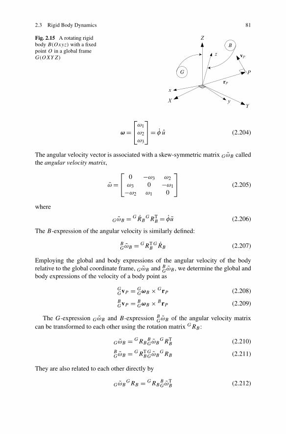
Consider a rotating rigid body B(Oxyz) with a fixed point O in a reference frameG(OXYZ), as shown in Fig. 2.15. We express the motion of the body by a time-varying rotation transformation matrix between B and G to transform the instanta-neous coordinates of body points to their coordinates in the global frame:
Gr(t) = GRB(t)Br (2.202)
The velocity of a body point in the global frame is
Gv(t) = Gr(t) = GRB(t)Br = GωBGr(t) = GωB × Gr(t) (2.203)
where GωB is the angular velocity vector of B with respect to G. It is equal to arotation with angular speed φ about an instantaneous axis of rotation u:
2.3 Rigid Body Dynamics 81
Fig. 2.15 A rotating rigidbody B(Oxyz) with a fixedpoint O in a global frameG(OXYZ)
ω =⎡
⎣ω1ω2ω3
⎤
⎦ = φ u (2.204)
The angular velocity vector is associated with a skew-symmetric matrix GωB calledthe angular velocity matrix,
ω =⎡
⎣0 −ω3 ω2ω3 0 −ω1
−ω2 ω1 0
⎤
⎦ (2.205)
where
GωB = GRBGRT
B = φu (2.206)
The B-expression of the angular velocity is similarly defined:
BGωB = GRT
BGRB (2.207)
Employing the global and body expressions of the angular velocity of the bodyrelative to the global coordinate frame, GωB and B
GωB , we determine the global andbody expressions of the velocity of a body point as
GGvP = G
GωB × GrP (2.208)
BGvP = B
GωB × BrP (2.209)
The G-expression GωB and B-expression BGωB of the angular velocity matrix
can be transformed to each other using the rotation matrix GRB :
GωB = GRBBGωB
GRTB (2.210)
BGωB = GRT
BGGωB
GRB (2.211)
They are also related to each other directly by
GωBGRB = GRB
BGωT
B (2.212)

82 2 Vibration Dynamics
Fig. 2.16 A body fixed pointP at Br in the rotating bodyframe B
GRTBGωB = B
GωBGRT
B (2.213)
The relative angular velocity vectors of relatively moving rigid bodies can bedone only if all the angular velocities are expressed in one coordinate frame:
0ωn = 0ω1 + 01ω2 + 0
2ω3 + · · · + 0n−1ωn =
n∑
i=1
0i−1ωi (2.214)
The inverses of the angular velocity matrices GωB and BGωB are
Gω−1B = GRB
GR−1B (2.215)
BGω−1
B = GR−1B
GRB (2.216)
Proof Consider a rigid body with a fixed point O and an attached frame B(Oxyz)
as shown in Fig. 2.16. The body frame B is initially coincident with the global frameG. Therefore, the position vector of a body point P at the initial time t = t0 is
Gr(t0) = Br (2.217)
and at any other time is found by the associated transformation matrix GRB(t):
Gr(t) = GRB(t)Br = GRB(t)Gr(t0) (2.218)
The global time derivative of Gr is
Gv = Gr =Gd
dt
Gr(t) =Gd
dt
[GRB(t)Br
] =Gd
dt
[GRB(t)Gr(t0)
]
= GRB(t)Gr(t0) = GRB(t)Br (2.219)
Eliminating Br between (2.218) and (2.219) determines the velocity of the globalpoint in the global frame:
Gv = GRB(t)GRTB(t)Gr(t) (2.220)
2.3 Rigid Body Dynamics 83
We denote the coefficient of Gr(t) by GωB
GωB = GRBGRT
B (2.221)
and rewrite Eq. (2.220) as
Gv = GωBGr(t) (2.222)
or equivalently as
Gv = GωB × Gr(t) (2.223)
where GωB is the instantaneous angular velocity of the body B relative to the globalframe G as seen from the G-frame.
Transforming Gv to the body frame provides us with the body expression of thevelocity vector:
BGvP = GRT
BGv = GRT
BGωBGr = GRT
BGRB
GRTB
Gr
= GRTB
GRBBr (2.224)
We denote the coefficient of Br by BGωB
BGωB = GRT
BGRB (2.225)
and rewrite Eq. (2.224) as
BGvP = B
GωBBrP (2.226)
or equivalently as
BGvP = B
GωB × BrP (2.227)
where BGωB is the instantaneous angular velocity of B relative to the global frame
G as seen from the B-frame.The time derivative of the orthogonality condition, GRB
GRTB = I, introduces an
important identity,
GRBGRT
B + GRBGRT
B = 0 (2.228)
which can be used to show that the angular velocity matrix GωB = [GRBGRT
B ] isskew-symmetric:
GRBGRT
B = [GRB
GRTB
]T (2.229)
Generally speaking, an angular velocity vector is the instantaneous rotation ofa coordinate frame A with respect to another frame B that can be expressed in orseen from a third coordinate frame C. We indicate the first coordinate frame A bya right subscript, the second frame B by a left subscript, and the third frame C bya left superscript, C
BωA. If the left super and subscripts are the same, we only showthe subscript.

84 2 Vibration Dynamics
We can transform the G-expression of the global velocity of a body point P ,GvP , and the B-expression of the global velocity of the point P , B
GvP , to each otherusing a rotation matrix:
BGvP = BRG
GvP = BRGGωBGrP = BRGGωB
GRBBrP
= BRGGRB
GRTB
GRBBrP = BRG
GRBBrP
= GRTB
GRBBrP = B
GωBBrP = B
GωB × BrP (2.230)
GvP = GRBBGvP = GRB
BGωB
BrP = GRBBGωB
GRTB
GrP
= GRBGRT
BGRB
GRTB
GrP = GRBGRT
BGrP
= GωBGrP = GωB × GrP = GRB
(BGωB × BrP
)(2.231)
From the definitions of GωB and BGωB in (2.221) and (2.225) and comparing with
(2.230) and (2.231), we are able to transform the two angular velocity matrices by
GωB = GRBBGωB
GRTB (2.232)
BGωB = GRT
BGωBGRB (2.233)
and derive the following useful equations:
GRB = GωBGRB (2.234)
GRB = GRBBGωB (2.235)
GωBGRB = GRB
BGωB (2.236)
The angular velocity of B in G is negative of the angular velocity of G in B ifboth are expressed in the same coordinate frame:
GGωB = −G
B ωGGGωB = −G
BωG (2.237)
BGωB = −B
BωGBGωB = −B
BωG (2.238)
The vector GωB can always be expressed in the natural form
GωB = ωu (2.239)
with the magnitude ω and a unit vector u parallel to GωB that indicates the instan-taneous axis of rotation.
To show the addition of relative angular velocities in Eq. (2.214), we start froma combination of rotations,
0R2 = 0R11R2 (2.240)
and take the time derivative:
0R2 = 0R11R2 + 0R1
1R2 (2.241)
2.3 Rigid Body Dynamics 85
Substituting the derivative of the rotation matrices with
0R2 = 0ω20R2 (2.242)
0R1 = 0ω10R1 (2.243)
1R2 = 1ω21R2 (2.244)
results in
0ω20R2 = 0ω1
0R11R2 + 0R11ω2
1R2
= 0ω10R2 + 0R11ω2
0RT1
0R11R2
= 0ω10R2 + 0
1ω20R2 (2.245)
where
0R11ω20RT
1 = 01ω2 (2.246)
Therefore, we find
0ω2 = 0ω1 + 01ω2 (2.247)
which indicates that two angular velocities may be added when they are expressedin the same frame:
0ω2 = 0ω1 + 01ω2 (2.248)
The expansion of this equation for any number of angular velocities would beEq. (2.214).
Employing the relative angular velocity formula (2.248), we can find the relativevelocity formula of a point P in B2 at 0rP :
0v2 = 0ω20rP = (
0ω1 + 01ω2
)0rP = 0ω10rP + 0
1ω20rP
= 0v1 + 01v2 (2.249)
The angular velocity matrices GωB and BGωB are skew-symmetric and not invert-
ible. However, we can define their inverse by the rules
Gω−1B = GRB
GR−1B (2.250)
BGω−1
B = GR−1B
GRB (2.251)
to get
Gω−1B GωB = GωBGω−1
B = [I] (2.252)
BGω−1
BBGωB = B
GωBBGω−1
B = [I] (2.253)
�

86 2 Vibration Dynamics
Example 55 � (Rotation of a body point about a global axis) Consider a rigid bodyis turning about the Z-axis with a constant angular speed α = 10 deg/s. The globalvelocity of a body point at P(5,30,10) when the body is at α = 30 deg is
GvP = GRB(t)BrP
=Gd
dt
⎛
⎝
⎡
⎣cosα − sinα 0sinα cosα 0
0 0 1
⎤
⎦
⎞
⎠
⎡
⎣5
3010
⎤
⎦
= α
⎡
⎣− sinα − cosα 0cosα − sinα 0
0 0 0
⎤
⎦
⎡
⎣5
3010
⎤
⎦
= 10π
180
⎡
⎣− sin π
6 − cos π6 0
cos π6 − sin π
6 00 0 0
⎤
⎦
⎡
⎣53010
⎤
⎦ =⎡
⎣−4.97−1.86
0
⎤
⎦ (2.254)
The point P is now at
GrP = GRBBrP
=⎡
⎣cos π
6 − sin π6 0
sin π6 cos π
6 00 0 1
⎤
⎦
⎡
⎣53010
⎤
⎦ =⎡
⎣−10.6728.48
10
⎤
⎦ (2.255)
Example 56 � (Rotation of a global point about a global axis) A body point P atBrP = [5 30 10]T is turned α = 30 deg about the Z-axis. The global position of P
is at
GrP = GRBBrP
=⎡
⎣cos π
6 − sin π6 0
sin π6 cos π
6 00 0 1
⎤
⎦
⎡
⎣53010
⎤
⎦ =⎡
⎣−10.6728.48
10
⎤
⎦ (2.256)
If the body is turning with a constant angular speed α = 10 deg/s, the global velocityof the point P would be
GvP = GRBGRT
BGrP
= 10π
180
⎡
⎣−s π
6 −c π6 0
c π6 −s π
6 00 0 0
⎤
⎦
⎡
⎣c π
6 −s π6 0
s π6 c π
6 00 0 1
⎤
⎦T ⎡
⎣−10.6728.48
10
⎤
⎦
=⎡
⎣−4.97−1.86
0
⎤
⎦ (2.257)

2.3 Rigid Body Dynamics 87
Example 57 � (Simple derivative transformation formula) Consider a point P thatcan move in the body coordinate frame B(Oxyz). The body position vector BrP isnot constant, and, therefore, the B-expression of the G-velocity of such a point is
Gd
dt
BrP = BGrP =
Bd
dt
BrP + BGωB × BrP (2.258)
The result of Eq. (2.258) is used to define the transformation of the differentialoperator on a B-vector B� from the body to the global coordinate frame:
Gd
dt
B� = BG�=
Bd
dt
B�+ BGωB × B� (2.259)
However, special attention must be paid to the coordinate frame in which the vectorB� and the final result are expressed. The final result is B
G�, showing the global(G) time derivative expressed in the body frame (B) or simply the B-expressionof the G-derivative of B�. The vector B� may be any vector quantity such as po-sition, velocity, angular velocity, momentum, angular momentum, a time-varyingforce vector.
Equation (2.259) is called a simple derivative transformation formula and relatesthe derivative of a B-vector as it would be seen from the G-frame to its derivativeas seen from the B-frame. The derivative transformation formula (2.259) is moregeneral and can be applied to every vector for a derivative transformation betweenevery two relatively moving coordinate frames.
2.3.3 � Acceleration Kinematics
Consider a rotating rigid body B(Oxyz) with a fixed point O in a reference frameG(OXYZ) such as shown in Fig. 2.17. When the body rotates in G, the globalacceleration of a body point P is given by
Ga = Gv = Gr = GSBGr (2.260)
= GαB × Gr + GωB × (GωB × Gr
)(2.261)
= (GαB + Gω2
B
)Gr (2.262)
= GRBGRT
BGr (2.263)
where GαB is the angular acceleration vector of B relative to G,
GαB =Gd
dtGωB (2.264)
and GαB is the angular acceleration matrix
GαB = G˙ωB = GRB
GRTB + GRB
GRTB (2.265)
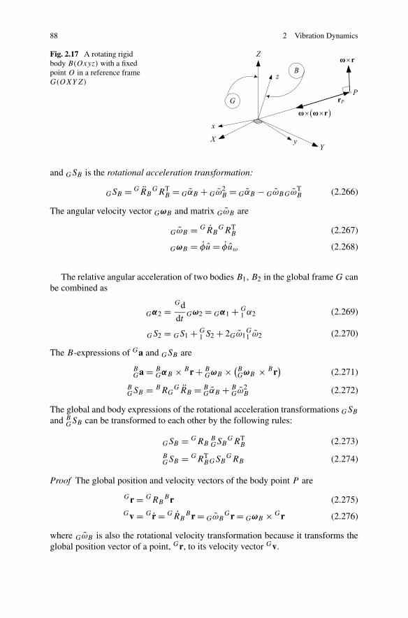
88 2 Vibration Dynamics
Fig. 2.17 A rotating rigidbody B(Oxyz) with a fixedpoint O in a reference frameG(OXYZ)
and GSB is the rotational acceleration transformation:
GSB = GRBGRT
B = GαB + Gω2B = GαB − GωBGωT
B (2.266)
The angular velocity vector GωB and matrix GωB are
GωB = GRBGRT
B (2.267)
GωB = φu = φuω (2.268)
The relative angular acceleration of two bodies B1, B2 in the global frame G canbe combined as
Gα2 =Gd
dtGω2 = Gα1 + G
1 α2 (2.269)
GS2 = GS1 + G1 S2 + 2Gω1
G1 ω2 (2.270)
The B-expressions of Ga and GSB are
BGa = B
GαB × Br + BGωB × (
BGωB × Br
)(2.271)
BGSB = BRG
GRB = BGαB + B
Gω2B (2.272)
The global and body expressions of the rotational acceleration transformations GSB
and BGSB can be transformed to each other by the following rules:
GSB = GRBBGSB
GRTB (2.273)
BGSB = GRT
BGSBGRB (2.274)
Proof The global position and velocity vectors of the body point P are
Gr = GRBBr (2.275)
Gv = Gr = GRBBr = GωB
Gr = GωB × Gr (2.276)
where GωB is also the rotational velocity transformation because it transforms theglobal position vector of a point, Gr, to its velocity vector Gv.
2.3 Rigid Body Dynamics 89
Differentiating Eq. (2.276) and using the notation GαB = Gddt GωB yield
Eq. (2.261):
Ga = Gr = GωB × Gr + GωB × Gr
= GαB × Gr + GωB × (GωB × Gr
)(2.277)
We may substitute the matrix expressions of angular velocity and acceleration in(2.277) to derive Eq. (2.262):
Gr = GαB × Gr + GωB × (GωB × Gr
)
= GαBGr + GωBGωB
Gr
= (GαB + Gω2
B
)Gr (2.278)
Recalling that
GωB = GRBGRT
B (2.279)
Gr(t) = GωBGr(t) (2.280)
we find Eqs. (2.263) and (2.265):
Gr =Gd
dt
(GRB
GRTB
Gr)
= GRBGRT
BGr + GRB
GRTB
Gr + [GRB
GRTB
][GRB
GRTB
]Gr
= [GRB
GRTB + GRB
GRTB + [G
RBGRT
B
]2]Gr
= [GRB
GRTB − [G
RBGRT
B
]2 + [GRB
GRTB
]2]Gr
= GRBGRT
BGr (2.281)
GαB = G˙ωB = GRB
GRTB + GRB
GRTB
= GRBGRT
B + GRBGRT
BGRB
GRTB
= GRBGRT
B + [GRB
GRTB
][GRB
GRTB
]T
= GRBGRT
B + GωBGωTB = GRB
GRTB − Gω2
B (2.282)
which indicates that
GRBGRT
B = GαB + Gω2B = GSB (2.283)

90 2 Vibration Dynamics
The expanded forms of the angular accelerations GαB , GαB and rotational ac-celeration transformation GSB are
GαB = G˙ωB = φu + φ ˙u =
⎡
⎣0 −ω3 ω2ω3 0 −ω1
−ω2 ω1 0
⎤
⎦
=⎡
⎣0 −u3φ − u3φ u2φ + u2φ
u3φ + u3φ 0 −u1φ − u1φ
−u2φ − u2φ u1φ + u1φ 0
⎤
⎦ (2.284)
GαB =⎡
⎣ω1ω2ω3
⎤
⎦ =⎡
⎣u1φ + u1φ
u2φ + u2φ
u3φ + u3φ
⎤
⎦ (2.285)
GSB = G˙ωB + Gω2
B = GαB + Gω2B
=⎡
⎣−ω2
2 − ω23 ω1ω2 − ω3 ω2 + ω1ω3
ω3 + ω1ω2 −ω21 − ω2
3 ω2ω3 − ω1
ω1ω3 − ω2 ω1 + ω2ω3 −ω21 − ω2
2
⎤
⎦ (2.286)
GSB = φu + φ ˙u + φ2u2
=⎡
⎣−(1 − u2
1)φ2 u1u2φ
2 − u3φ − u3φ u1u3φ2 + u2φ + u2φ
u1u2φ2 + u3φ + u3φ −(1 − u2
2)φ2 u2u3φ
2 − u1φ − u1φ
u1u3φ2 − u2φ − u2φ u2u3φ
2 + u1φ + u1φ −(1 − u23)φ
2
⎤
⎦
(2.287)
The angular velocity of several bodies rotating relative to each other can be re-lated according to (2.214):
0ωn = 0ω1 + 01ω2 + 0
2ω3 + · · · + 0n−1ωn (2.288)
The angular accelerations of several relatively rotating rigid bodies follow the samerule:
0αn = 0α1 + 01α2 + 0
2α3 + · · · + 0n−1αn (2.289)
To show this fact and develop the relative acceleration formula, we consider a pairof relatively rotating rigid links in a base coordinate frame B0 with a fixed point atO . The angular velocities of the links are related as
0ω2 = 0ω1 + 01ω2 (2.290)
So, their angular accelerations are
0α1 =0d
dt0ω1 (2.291)
2.3 Rigid Body Dynamics 91
0α2 =0d
dt0ω2 = 0α1 + 0
1α2 (2.292)
and, therefore,
0S2 = 0α2 + 0ω22 = 0α1 + 0
1α2 + (0ω1 + 0
1ω2)2
= 0α1 + 01α2 + 0ω
21 + 0
1ω22 + 20ω1
01ω2
= 0S1 + 01S2 + 20ω1
01ω2 (2.293)
Equation (2.293) is the required relative acceleration transformation formula. Itindicates the method of calculation of relative accelerations for a multibody. As amore general case, consider a six-link multibody. The angular acceleration of link(6) in the base frame would be
0S6 = 0S1 + 01S2 + 0
2S3 + 03S4 + 0
4S5 + 05S6
+ 20ω1(0
1ω2 + 02ω3 + 0
3ω4 + 04ω5 + 0
5ω6)
+ 201ω2
(02ω3 + 0
3ω4 + 04ω5 + 0
5ω6)
...
+ 204ω5
(05ω6
)(2.294)
We can transform the G and B-expressions of the global acceleration of a bodypoint P to each other using a rotation matrix:
BGaP = BRG
GaP = BRGGSBGrP = BRG GSB
GRBBrP
= BRGGRB
GRTB
GRBBrP = BRG
GRBBrP
= GRTB
GRBBrP = B
GSBBrP = (B
GαB + B
Gω2B
)BrP
= BGαB × Br + B
GωB × (BGωB × Br
)(2.295)
GaP = GRBBGaP = GRB
BGSB
BrP = GRBBGSB
GRTB
GrP
= GRBGRT
BGRB
GRTB
GrP = GRBGRT
BGrP
= GSBGrP = (
GαB + Gω2
B
)Gr
= GαB × Gr + GωB × (GωB × Gr
)(2.296)
From the definitions of GSB and BGSB in (2.266) and (2.272) and comparing with
(2.295) and (2.296), we are able to transform the two rotational acceleration trans-formations by
GSB = GRBBGSB
GRTB (2.297)
92 2 Vibration Dynamics
BGSB = GRT
BGSBGRB (2.298)
and derive the useful equations
GRB = GSBGRB (2.299)
GRB = GRBBGSB (2.300)
GSBGRB = GRB
BGSB (2.301)
The angular acceleration of B in G is negative of the angular acceleration of G
in B if both are expressed in the same coordinate frame:
GαB = −GB αG GαB = −G
BαG (2.302)
BGαB = −BαG
BGαB = −BαG (2.303)
The term GαB × Gr in (2.277) is called the tangential acceleration, which is afunction of the angular acceleration of B in G. The term GωB × (GωB × Gr) inGa is called centripetal acceleration and is a function of the angular velocity of B
in G. �
Example 58 � (Rotation of a body point about a global axis) Consider a rigidbody is turning about the Z-axis with a constant angular acceleration α = 2 rad/s2.The global acceleration of a body point at P(5,30,10) cm when the body is atα = 10 rad/s and α = 30 deg is
GaP = GRB(t)BrP
=⎡
⎣−87.6 48.27 0−48.27 −87.6 0
0 0 0
⎤
⎦
⎡
⎣5
3010
⎤
⎦ =⎡
⎣1010
−2869.40
⎤
⎦ cm/s (2.304)
where
GRB =Gd2
dt2GRB = α
Gd
dα
GRB = αGd
dα
GRB + α2Gd2
dα2GRB
= α
⎡
⎣− sinα − cosα 0cosα − sinα 0
0 0 0
⎤
⎦+ α2
⎡
⎣− cosα sinα 0− sinα − cosα 0
0 0 0
⎤
⎦ (2.305)
At this moment, the point P is at
GrP = GRBBrP
=⎡
⎣cos π
6 − sin π6 0
sin π6 cos π
6 00 0 1
⎤
⎦
⎡
⎣53010
⎤
⎦ =⎡
⎣−10.6728.48
10
⎤
⎦ cm (2.306)
2.3 Rigid Body Dynamics 93
Example 59 � (Rotation of a global point about a global axis) A body point P atBrP = [5 30 10]T cm is turning with a constant angular acceleration α = 2 rad/s2
about the Z-axis. When the body frame is at α = 30 deg, its angular speedα = 10 deg/s.
The transformation matrix GRB between the B- and G-frames is
GRB =⎡
⎣cos π
6 − sin π6 0
sin π6 cos π
6 00 0 1
⎤
⎦ ≈⎡
⎣0.866 −0.5 0
0.5 0.866 00 0 1
⎤
⎦ (2.307)
and, therefore, the acceleration of point P is
GaP = GRBGRT
BGrP =
⎡
⎣1010
−2869.40
⎤
⎦ cm/s2 (2.308)
whereGd2
dt2GRB = α
Gd
dα
GRB − α2Gd2
dα2GRB (2.309)
is the same as (2.305).
Example 60 � (B-expression of angular acceleration) The angular acceleration ex-pressed in the body frame is the body derivative of the angular velocity vector. Toshow this, we use the derivative transport formula (2.259):
BGαB = B
GωB =Gd
dt
BGωB
=Bd
dt
BGωB + B
GωB × BGωB =
Bd
dt
BGωB (2.310)
Interestingly, the global and body derivatives of BGωB are equal:
Gd
dt
BGωB =
Bd
dt
BGωB = B
GαB (2.311)
This is because GωB is about an axis u that is instantaneously fixed in both B and G.A vector α can generally indicate the angular acceleration of a coordinate frame
A with respect to another frame B . It can be expressed in or seen from a thirdcoordinate frame C. We indicate the first coordinate frame A by a right subscript,the second frame B by a left subscript, and the third frame C by a left superscript,CBαA. If the left super and subscripts are the same, we only show the subscript. So,the angular acceleration of A with respect to B as seen from C is the C-expressionof BαA:
CBαA = CRBBαA (2.312)
94 2 Vibration Dynamics
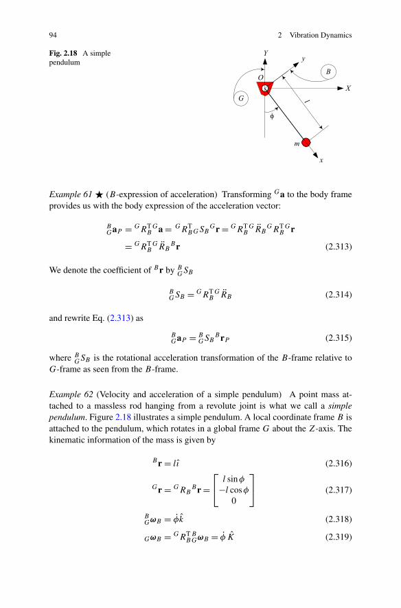
Fig. 2.18 A simplependulum
Example 61 � (B-expression of acceleration) Transforming Ga to the body frameprovides us with the body expression of the acceleration vector:
BGaP = GRT
BGa = GRT
BGSBGr = GRT
BGRB
GRTB
Gr
= GRTB
GRBBr (2.313)
We denote the coefficient of Br by BGSB
BGSB = GRT
BGRB (2.314)
and rewrite Eq. (2.313) as
BGaP = B
GSBBrP (2.315)
where BGSB is the rotational acceleration transformation of the B-frame relative to
G-frame as seen from the B-frame.
Example 62 (Velocity and acceleration of a simple pendulum) A point mass at-tached to a massless rod hanging from a revolute joint is what we call a simplependulum. Figure 2.18 illustrates a simple pendulum. A local coordinate frame B isattached to the pendulum, which rotates in a global frame G about the Z-axis. Thekinematic information of the mass is given by
Br = lı (2.316)
Gr = GRBBr =
⎡
⎣l sinφ
−l cosφ
0
⎤
⎦ (2.317)
BGωB = φk (2.318)
GωB = GRTB
BGωB = φ K (2.319)
2.3 Rigid Body Dynamics 95
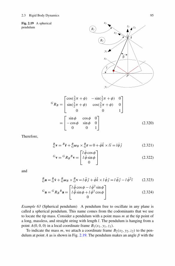
Fig. 2.19 A sphericalpendulum
GRB =⎡
⎢⎣cos( 3
2π + φ) − sin( 32π + φ) 0
sin( 32π + φ) cos( 3
2π + φ) 0
0 0 1
⎤
⎥⎦
=⎡
⎣sinφ cosφ 0
− cosφ sinφ 00 0 1
⎤
⎦ (2.320)
Therefore,
BGv = B r + B
GωB × BGr = 0 + φk × lı = lφj (2.321)
Gv = GRBBv =
⎡
⎣l φ cosφ
l φ sinφ
0
⎤
⎦ (2.322)
and
BGa = B
Gv + BGωB × B
Gv = l φj + φk × l φj = l φj − l φ2 ı (2.323)
Ga = GRBBa =
⎡
⎣l φ cosφ − l φ2 sinφ
l φ sinφ + l φ2 cosφ
0
⎤
⎦ (2.324)
Example 63 (Spherical pendulum) A pendulum free to oscillate in any plane iscalled a spherical pendulum. This name comes from the codominants that we useto locate the tip mass. Consider a pendulum with a point mass m at the tip point ofa long, massless, and straight string with length l. The pendulum is hanging from apoint A(0,0,0) in a local coordinate frame B1(x1, y1, z1).
To indicate the mass m, we attach a coordinate frame B2(x2, y2, z2) to the pen-dulum at point A as is shown in Fig. 2.19. The pendulum makes an angle β with the
96 2 Vibration Dynamics
vertical z1-axis. The pendulum swings in the plane (x2, z2) and makes an angle γ
with the plane (x1, z1). Therefore, the transformation matrix between B2 and B1 is
2R1 = Ry2,−β Rz2,γ
=⎡
⎣cosγ cosβ cosβ sinγ sinβ
− sinγ cosγ 0− cosγ sinβ − sinγ sinβ cosβ
⎤
⎦ (2.325)
The position vectors of m are
2r =⎡
⎣00−l
⎤
⎦ 1r = 1R22r =
⎡
⎣l cosγ sinβ
l sinβ sinγ
−l cosβ
⎤
⎦ (2.326)
The equation of motion of m is
1M = I 1α2 (2.327)1r × m1g = ml2
1α2 (2.328)⎡
⎣l cosγ sinβ
l sinβ sinγ
−l cosβ
⎤
⎦× m
⎡
⎣00
−g0
⎤
⎦ = ml21α2 (2.329)
Therefore,
1α2 = g0
l
⎡
⎣− sinβ sinγ
cosγ sinβ
0
⎤
⎦ (2.330)
To find the angular acceleration of B2 in B1, we use 2R1:
1R2 = βd
dβ
2R1 + γd
dγ
2R1
=⎡
⎣−βcγ sβ − γ cβsγ −γ cγ γ sβsγ − βcβcγ
γ cβcγ − βsβsγ −γ sγ −βcβsγ − γ cγ sβ
βcβ 0 −βsβ
⎤
⎦ (2.331)
1ω2 = 1R21RT
2 =⎡
⎣0 −γ −β cosγ
γ 0 −β sinγ
β cosγ β sinγ 0
⎤
⎦ (2.332)
1R2 = βd
dβ
2R1 + β2 d2
dβ22R1 + βγ
d2
dγ dβ
2R1
+ γd
dγ
2R1 + γ βd2
dβ dγ
2R1 + γ 2 d2
dγ 22R1 (2.333)

2.3 Rigid Body Dynamics 97
1α2 = 1R21RT
2 − 1ω22
=⎡
⎣0 −γ −βcγ + βγ sγ
γ 0 −βsγ − βγ cγ
βcγ − βγ sγ βsγ + βγ cγ 0
⎤
⎦ (2.334)
Therefore, the equation of motion of the pendulum would be
g0
l
⎡
⎣− sinβ sinγ
cosγ sinβ
0
⎤
⎦ =⎡
⎣β sinγ + βγ cosγ
−β cosγ + βγ sinγ
γ
⎤
⎦ (2.335)
The third equation indicates that
γ = γ0 γ = γ0t + γ0 (2.336)
The second and third equations can be combined to form
β = −√
g20
l2sin2 β + β2γ 2
0 (2.337)
which reduces to the equation of a simple pendulum if γ0 = 0.
Example 64 � (Equation of motion of a spherical pendulum) Consider a particleP of mass m that is suspended by a string of length l from a point A, as shown inFig. 2.19. If we show the tension of the string by T, then the equation of motion ofP is
1T + m1g = m1r (2.338)
or −T 1r + m1g = m1r. To eliminate 1T, we multiply the equation by 1r,
1r × 1g = 1r × 1r⎡
⎣l cosγ sinβ
l sinβ sinγ
−l cosβ
⎤
⎦×⎡
⎣00
−g0
⎤
⎦ =⎡
⎣l cosγ sinβ
l sinβ sinγ
−l cosβ
⎤
⎦×⎡
⎣x
y
z
⎤
⎦(2.339)
and find⎡
⎣−lg0 sinβ sinγ
lg0 cosγ sinβ
0
⎤
⎦ =⎡
⎣ly cosβ + lz sinβ sinγ
−lx cosβ − lz cosγ sinβ
ly cosγ − lx sinγ
⎤
⎦ (2.340)
These are the equations of motion of m. However, we may express the equationsonly in terms of γ and β . To do so, we may either take time derivatives of 1r or use1α2 from Example 64 and find 1r:
1r = 1α2 × 1r (2.341)
In either case, Eq. (2.335) would be the equation of motion in terms of γ and β .

98 2 Vibration Dynamics
Fig. 2.20 Foucault pendulumis a simple pendulum hangingfrom a point A above a pointP on Earth surface
Example 65 � (Foucault pendulum) Consider a pendulum with a point mass m
at the tip of a long, massless, and straight string with length l. The pendulum ishanging from a point A(0,0, l) in a local coordinate frame B1(x1, y1, z1) at a pointP on the Earth surface. Point P at longitude ϕ and latitude λ is indicated by Edin the Earth frame E(Oxyz). The E-frame is turning in a global frame G(OXYZ)
about the Z-axis.To indicate the mass m, we attach a coordinate frame B1(x1, y1, z1) to the pen-
dulum at point A as shown in Fig. 2.20. The pendulum makes an angle β with thevertical z1-axis. The pendulum swings in the plane (x2, z2) and makes an angle γ
with the plane (x1, z1). Therefore, the transformation matrix between B2 and B1 is
1T2 = 1D21R2
=
⎡
⎢⎢⎣
cosγ cosβ − sinγ − cosγ sinβ 0cosβ sinγ cosγ − sinγ sinβ 0
sinβ 0 cosβ l
0 0 0 1
⎤
⎥⎥⎦ (2.342)
The position vector of m is
2r =⎡
⎣00−l
⎤
⎦ (2.343)
1r = 1T22r =
⎡
⎣x1y1z1
⎤
⎦ =⎡
⎣l cosγ sinβ
l sinβ sinγ
l − l cosβ
⎤
⎦ (2.344)
Employing the acceleration equation,
1Ga = 1a + 1
Gα1 × 1r + 21Gω1 × 1v + 1
Gω1 × (1Gω1 × 1r
)(2.345)
2.3 Rigid Body Dynamics 99
we can write the equation of motion of m as
1GF − m1
Gg = m1Ga (2.346)
where 1F is the applied nongravitational force on m.Recalling that
1Gα1 = 0 (2.347)
we find the general equation of motion of a particle in frame B1 as
1GF + m1
Gg = m(1a + 21
Gω1 × 1v + 1Gω1 × (1
Gω1 × 1r))
(2.348)
The individual vectors in this equation are
1g =⎡
⎣00
−g0
⎤
⎦ 1GF =
⎡
⎣Fx
Fy
Fz
⎤
⎦ 1Gω1 =
⎡
⎣ωE cosλ
0ωE sinλ
⎤
⎦ (2.349)
1v =⎡
⎣x1y1z1
⎤
⎦ =⎡
⎣lβ cosβ cosγ − lγ sinβ sinγ
lβ cosβ sinγ + lγ cosγ sinβ
lβ sinβ
⎤
⎦ (2.350)
1a =⎡
⎣x
y
z
⎤
⎦ =
⎡
⎢⎢⎢⎢⎣
l(β cosγ − β2 sinγ − βγ sinγ ) cosβ
− l(γ sinγ + γ 2 cosγ + βγ cosγ ) sinβ
l(β sinγ + β2 cosγ + βγ cosγ ) cosβ
+ l(γ cosγ − γ 2 sinγ − βγ sinγ ) sinβ
lβ sinβ
⎤
⎥⎥⎥⎥⎦(2.351)
In a spherical pendulum, the external force 1F is the tension of the string:
1GF = −F
l
1r (2.352)
Substituting the above vectors in (2.348) provides us with three coupled ordinarydifferential equations for two angular variables γ and β . One of the equations is notindependent and the others may theoretically be integrated to determine γ = γ (t)
and β = β(t).For example, let us use
ωE ≈ 7.292 1 × 10⁻⁵ rad/s
g0 ≈ 9.81 m/s2
l = 100 m
λ = 28◦58′30′′N ≈ 28.975 deg N
ϕ = 50◦50′17′′E ≈ 50.838 deg E
x0 = l cos 10 = 17.365 m (2.353)
100 2 Vibration Dynamics
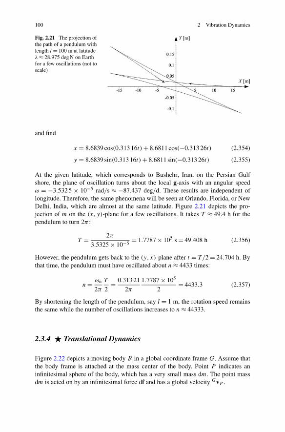
Fig. 2.21 The projection ofthe path of a pendulum withlength l = 100 m at latitudeλ ≈ 28.975 deg N on Earthfor a few oscillations (not toscale)
and find
x = 8.6839 cos(0.313 16t) + 8.6811 cos(−0.313 26t) (2.354)
y = 8.6839 sin(0.313 16t) + 8.6811 sin(−0.313 26t) (2.355)
At the given latitude, which corresponds to Bushehr, Iran, on the Persian Gulfshore, the plane of oscillation turns about the local g-axis with an angular speedω = −3.532 5 × 10⁻⁵ rad/s ≈ −87.437 deg/d. These results are independent oflongitude. Therefore, the same phenomena will be seen at Orlando, Florida, or NewDelhi, India, which are almost at the same latitude. Figure 2.21 depicts the pro-jection of m on the (x, y)-plane for a few oscillations. It takes T ≈ 49.4 h for thependulum to turn 2π :
T = 2π
3.5325 × 10−5= 1.7787 × 10⁵ s = 49.408 h (2.356)
However, the pendulum gets back to the (y, x)-plane after t = T/2 = 24.704 h. Bythat time, the pendulum must have oscillated about n ≈ 4433 times:
n = ωn
2π
T
2= 0.313 21
2π
1.7787 × 10⁵
2= 4433.3 (2.357)
By shortening the length of the pendulum, say l = 1 m, the rotation speed remainsthe same while the number of oscillations increases to n ≈ 44333.
2.3.4 � Translational Dynamics
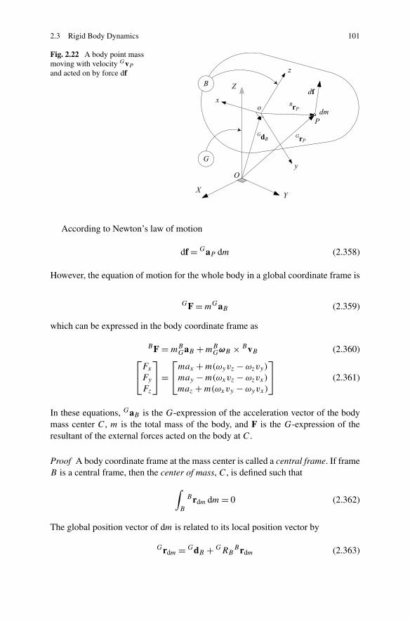
Figure 2.22 depicts a moving body B in a global coordinate frame G. Assume thatthe body frame is attached at the mass center of the body. Point P indicates aninfinitesimal sphere of the body, which has a very small mass dm. The point massdm is acted on by an infinitesimal force df and has a global velocity GvP .
2.3 Rigid Body Dynamics 101
Fig. 2.22 A body point massmoving with velocity GvP
and acted on by force df
According to Newton’s law of motion
df = GaP dm (2.358)
However, the equation of motion for the whole body in a global coordinate frame is
GF = mGaB (2.359)
which can be expressed in the body coordinate frame as
BF = mBGaB + mB
GωB × BvB (2.360)⎡
⎣Fx
Fy
Fz
⎤
⎦ =⎡
⎣max + m(ωyvz − ωzvy)
may − m(ωxvz − ωzvx)
maz + m(ωxvy − ωyvx)
⎤
⎦ (2.361)
In these equations, GaB is the G-expression of the acceleration vector of the bodymass center C, m is the total mass of the body, and F is the G-expression of theresultant of the external forces acted on the body at C.
Proof A body coordinate frame at the mass center is called a central frame. If frameB is a central frame, then the center of mass, C, is defined such that
∫
B
Brdm dm = 0 (2.362)
The global position vector of dm is related to its local position vector by
Grdm = GdB + GRBBrdm (2.363)
102 2 Vibration Dynamics
where GdB is the global position vector of the central body frame, and, therefore,
∫
B
Grdm dm =∫
B
GdB dm + GRB
∫
m
Brdm dm
=∫
B
GdB dm = GdB
∫
B
dm = mGdB (2.364)
The time derivative of both sides shows that
mGdB = mGvB =∫
B
Grdm dm =∫
B
Gvdm dm (2.365)
and the other derivative is
mGvB = mGaB =∫
B
Gvdm dm (2.366)
However, we have df = GvP dm and, therefore,
mGaB =∫
B
df (2.367)
The integral on the right-hand side collects all the forces acting on the body. Theinternal forces cancel one another out, so the net result is the vector sum of all theexternally applied forces, F, and, therefore,
GF = mGaB = mGvB (2.368)
In the body coordinate frame we have
BF = BRGGF = mBRG
GaB = mBGaB
= mBaB + mBGωB × BvB (2.369)
The expanded form of Newton’s equation in the body coordinate frame is then equalto
BF = mBaB + mBGωB × BvB
⎡
⎣Fx
Fy
Fz
⎤
⎦ = m
⎡
⎣ax
ay
az
⎤
⎦+ m
⎡
⎣ωx
ωy
ωz
⎤
⎦×⎡
⎣vx
vy
vz
⎤
⎦
=⎡
⎣max + m(ωyvz − ωzvy)
may − m(ωxvz − ωzvx)
maz + m(ωxvy − ωyvx)
⎤
⎦ (2.370)
�
2.3 Rigid Body Dynamics 103
2.3.5 � Rotational Dynamics
The rigid body rotational equation of motion is the Euler equation
BM =Gd
dt
BL = B L + BGωB × BL
= BIBGωB + B
GωB × (BIB
GωB
)(2.371)
where L is the angular momentum
BL = BIBGωB (2.372)
and I is the mass moment of the rigid body.
I =⎡
⎣Ixx Ixy Ixz
Iyx Iyy Iyz
Izx Izy Izz
⎤
⎦ (2.373)
The expanded form of the Euler equation (2.371) is
Mx = Ixxωx + Ixyωy + Ixzωz − (Iyy − Izz)ωyωz
−Iyz
(ω2
z − ω2y
)− ωx(ωzIxy − ωyIxz) (2.374)
My = Iyxωx + Iyyωy + Iyzωz − (Izz − Ixx)ωzωx
−Ixz
(ω2
x − ω2z
)− ωy(ωxIyz − ωzIxy) (2.375)
Mz = Izxωx + Izyωy + Izzωz − (Ixx − Iyy)ωxωy
−Ixy
(ω2
y − ω2x
)− ωz(ωyIxz − ωxIyz) (2.376)
which can be reduced to
M1 = I1ω1 − (I2 − I2)ω2ω3
M2 = I2ω2 − (I3 − I1)ω3ω1 (2.377)
M3 = I3ω3 − (I1 − I2)ω1ω2
when the body coordinate is the principal coordinate frame. The principal coordi-nate frame is denoted by numbers 123 to indicate the first, second, and third princi-pal axes. The parameters Iij , i �= j , are zero in the principal frame. The body andprincipal coordinate frame sit at the mass center C.
The kinetic energy of a rotating rigid body is
K = 1
2
(Ixxω
2x + Iyyω
2y + Izzω
2z
)
− Ixyωxωy − Iyzωyωz − Izxωzωx (2.378)

104 2 Vibration Dynamics
= 1
2ω · L = 1
2ωTI ω (2.379)
which in the principal coordinate frame reduces to
K = 1
2
(I1ω
21 + I2ω
22 + I3ω
23
)(2.380)
Proof Let mi be the mass of the ith particle of a rigid body B , which is made of n
particles and let
ri = Bri = [xi yi zi
]T (2.381)
be the Cartesian position vector of mi in a central body fixed coordinate frameB(Oxyz). Assume that
ω = BGωB = [
ωx ωy ωz
]T (2.382)
is the angular velocity of the rigid body with respect to the global coordinate frameG(OXYZ), expressed in the body coordinate frame.
The angular momentum of mi is
Li = ri × mi ri = mi
[ri × (ω × ri )
]
= mi
[(ri · ri )ω − (ri · ω)ri
]
= mir2i ω − mi(ri · ω)ri (2.383)
Hence, the angular momentum of the rigid body would be
L = ω
n∑
i=1
mir2i −
n∑
i=1
mi(ri · ω)ri (2.384)
Substitution for ri and ω gives us
L = (ωx ı + ωyj + ωzk)
n∑
i=1
mi
(x2i + y2
i + z2i
)
−n∑
i=1
mi(xiωx + yiωy + ziωz) · (xi ı + yi j + zi k) (2.385)
which can be rearranged as
L =n∑
i=1
mi
(y2i + z2
i
)ωxı +
n∑
i=1
mi
(z2i + x2
i
)ωyj +
n∑
i=1
mi
(x2i + y2
i
)ωzk
−(
n∑
i=1
(mixiyi)ωy +n∑
i=1
(mixizi)ωz
)ı

2.3 Rigid Body Dynamics 105
−(
n∑
i=1
(miyizi)ωz +n∑
i=1
(miyixi)ωx
)j
−(
n∑
i=1
(mizixi)ωx +n∑
i=1
(miziyi)ωy
)k (2.386)
By introducing the mass moment matrix I with the following elements:
Ixx =n∑
i=1
[mi
(y2i + z2
i
)](2.387)
Iyy =n∑
i=1
[mi
(z2i + x2
i
)](2.388)
Izz =n∑
i=1
[mi
(x2i + y2
i
)](2.389)
Ixy = Iyx = −n∑
i=1
(mixiyi) (2.390)
Iyz = Izy = −n∑
i=1
(miyizi) (2.391)
Izx = Ixz = −n∑
i=1
(mizixi) (2.392)
we may write the angular momentum L in concise form:
Lx = Ixxωx + Ixyωy + Ixzωz (2.393)
Ly = Iyxωx + Iyyωy + Iyzωz (2.394)
Lz = Izxωx + Izyωy + Izzωz (2.395)
or in matrix form:
L = I · ω (2.396)⎡
⎣Lx
Ly
Lz
⎤
⎦ =⎡
⎣Ixx Ixy Ixz
Iyx Iyy Iyz
Izx Izy Izz
⎤
⎦
⎡
⎣ωx
ωy
ωz
⎤
⎦ (2.397)
For a rigid body that is a continuous solid, the summations must be replaced byintegrations over the volume of the body as in Eq. (2.433).

106 2 Vibration Dynamics
The Euler equation of motion for a rigid body is
BM =Gd
dt
BL (2.398)
where BM is the resultant of the external moments applied on the rigid body. Theangular momentum BL is a vector quantity defined in the body coordinate frame.Hence, its time derivative in the global coordinate frame is
GdBLdt
= B L + BGωB × BL (2.399)
Therefore,
BM = dLdt
= L + ω × L = I ω + ω × (Iω) (2.400)
or in expanded form
BM = (Ixxωx + Ixyωy + Ixzωz)ı + ωy(Ixzωx + Iyzωy + Izzωz)ı
− ωz(Ixyωx + Iyyωy + Iyzωz)ı
+ (Iyxωx + Iyyωy + Iyzωz)j + ωz(Ixxωx + Ixyωy + Ixzωz)j
− ωx(Ixzωx + Iyzωy + Izzωz)j
+ (Izxωx + Izyωy + Izzωz)k + ωx(Ixyωx + Iyyωy + Iyzωz)k
− ωy(Ixxωx + Ixyωy + Ixzωz)k (2.401)
and, therefore, the most general form of the Euler equations of motion for a rigidbody in a body frame attached to C are
Mx = Ixxωx + Ixyωy + Ixzωz − (Iyy − Izz)ωyωz
− Iyz
(ω2
z − ω2y
)− ωx(ωzIxy − ωyIxz) (2.402)
My = Iyxωx + Iyyωy + Iyzωz − (Izz − Ixx)ωzωx
− Ixz
(ω2
x − ω2z
)− ωy(ωxIyz − ωzIxy) (2.403)
Mz = Izxωx + Izyωy + Izzωz − (Ixx − Iyy)ωxωy
− Ixy
(ω2
y − ω2x
)− ωz(ωyIxz − ωxIyz) (2.404)
Assume that we are able to rotate the body frame about its origin to find an orien-tation that makes Iij = 0, for i �= j . In such a coordinate frame, which is called aprincipal frame, the Euler equations reduce to
M1 = I1ω1 − (I2 − I2)ω2ω3 (2.405)
M2 = I2ω2 − (I3 − I1)ω3ω1 (2.406)

2.3 Rigid Body Dynamics 107
Fig. 2.23 A disc with massm and radius r , mounted on amassless turning shaft
M3 = I3ω3 − (I1 − I2)ω1ω2 (2.407)
The kinetic energy of a rigid body may be found by the integral of the kineticenergy of the mass element dm, over the whole body:
K = 1
2
∫
B
v2 dm = 1
2
∫
B
(ω × r) · (ω × r)dm
= ω2x
2
∫
B
(y2 + z2)dm + ω2
y
2
∫
B
(z2 + x2)dm + ω2
z
2
∫
B
(x2 + y2)dm
− ωxωy
∫
B
xy dm − ωyωz
∫
B
yzdm − ωzωx
∫
B
zx dm
= 1
2
(Ixxω
2x + Iyyω
2y + Izzω
2z
)
− Ixyωxωy − Iyzωyωz − Izxωzωx (2.408)
The kinetic energy can be rearranged to a matrix multiplication form
K = 1
2ωTI ω = 1
2ω · L (2.409)
When the body frame is principal, the kinetic energy will simplify to
K = 1
2
(I1ω
21 + I2ω
22 + I3ω
23
)(2.410)
�
Example 66 � (A tilted disc on a massless shaft) Figure 2.23 illustrates a disc withmass m and radius R, mounted on a massless shaft. The shaft is turning with aconstant angular speed ω. The disc is attached to the shaft at an angle α. Because ofα, the bearings at A and B must support a rotating force.
We attach a principal body coordinate frame at the disc center as shown in thefigure. The G-expression of the angular velocity is a constant vector
GωB = ωI (2.411)
108 2 Vibration Dynamics
and the expression of the angular velocity vector in the body frame is
BGωB = ω cos θ ı + ω sin θ j (2.412)
The mass moment of inertia matrix is
BI =⎡
⎣mR2/2 0 0
0 mR2/4 00 0 mR2/4
⎤
⎦ (2.413)
Substituting (2.412) and (2.413) in (2.405)–(2.407), with 1 ≡ x, 2 ≡ y, 3 ≡ z, yields
Mx = 0 (2.414)
My = 0 (2.415)
Mz = mr2
4ω cos θ sin θ (2.416)
Therefore, the bearing reaction forces FA and FB are
FA = −FB = −Mz
l= −mr2
4lω cos θ sin θ (2.417)
Example 67 (Steady rotation of a freely rotating rigid body) Consider a situation inwhich the resultant applied force and moment on a rigid body are zero:
GF = BF = 0 (2.418)
GM = BM = 0 (2.419)
Based on Newton’s equation,
GF = mGv (2.420)
the velocity of the mass center will be constant in the global coordinate frame. How-ever, the Euler equation
BM = IBGωB + B
GωB × BL (2.421)
reduces to
ω1 = I2 − I3
I1ω2ω3 (2.422)
ω2 = I3 − I1
I22ω3ω1 (2.423)
ω3 = I1 − I2
I3ω1ω2 (2.424)
2.3 Rigid Body Dynamics 109
which show that the angular velocity can be constant if
I1 = I2 = I3 (2.425)
or if two principal moments of inertia, say I1 and I2, are zero and the third angularvelocity, in this case ω3, is initially zero, or if the angular velocity vector is initiallyparallel to a principal axis.
2.3.6 � Mass Moment Matrix
Two types of integral arise in rigid body dynamics that depend solely on the geome-try and mass distribution of the body. The first type defines the center of mass and isimportant when the translation motion of the body is considered. The second is themass moment, which appears when the rotational motion of the body is considered.The mass moment is also called moment of inertia, centrifugal moments, or devia-tion moment. Every rigid body has a 3 × 3 mass moment matrix I , which is denotedby
I =⎡
⎣Ixx Ixy Ixz
Iyx Iyy Iyz
Izx Izy Izz
⎤
⎦ (2.426)
The diagonal elements Iij , i = j , are called polar mass moments
Ixx = Ix =∫
B
(y2 + z2)dm (2.427)
Iyy = Iy =∫
B
(z2 + x2)dm (2.428)
Izz = Iz =∫
B
(x2 + y2)dm (2.429)
and the off-diagonal elements Iij , i �= j , are called products of inertia
Ixy = Iyx = −∫
B
xy dm (2.430)
Iyz = Izy = −∫
B
yzdm (2.431)
Izx = Ixz = −∫
B
zx dm (2.432)
The elements of I are functions of the mass distribution of the rigid body and maybe defined by
Iij =∫
B
(r2i δmn − ximxjn
)dm i, j = 1,2,3 (2.433)
110 2 Vibration Dynamics
where δij is Kronecker’s delta (2.171),
δmn ={
1 if m = n
0 if m �= n(2.434)
The elements of I are calculated in a body coordinate frame attached to the masscenter C of the body. Therefore, I is a frame-dependent quantity and must be writtenwith a frame indicator such as BI to show the frame in which it is computed:
BI =∫
B
⎡
⎣y2 + z2 −xy −zx
−xy z2 + x2 −yz
−zx −yz x2 + y2
⎤
⎦ dm (2.435)
=∫
B
(r2I − r rT)dm =
∫
B
−r r dm (2.436)
where r is the associated skew-symmetric matrix of r:
r =⎡
⎣0 −r3 r2r3 0 −r1
−r2 r1 0
⎤
⎦ (2.437)
The moments of inertia can be transformed from a coordinate frame B1 to an-other coordinate frame B2, both defined at the mass center of the body, according tothe rule of the rotated-axes theorem:
B2I = B2RB1B1IB2RT
B1(2.438)
Transformation of the moment of inertia from a central frame B1 located at B2 rC toanother frame B2, which is parallel to B1, is, according to the rule of the parallel-axes theorem:
B2I = B1I + mrC rTC (2.439)
If the local coordinate frame Oxyz is located such that the products of inertiavanish, the local coordinate frame is the principal coordinate frame and the associ-ated mass moments are principal mass moments. Principal axes and principal massmoments can be found by solving the following characteristic equation for I :
∣∣∣∣∣∣
Ixx − I Ixy Ixz
Iyx Iyy − I Iyz
Izx Izy Izz − I
∣∣∣∣∣∣= 0 (2.440)
det([Iij ] − I [δij ]
) = 0 (2.441)
Equation (2.441) is a cubic equation in I , so we obtain three eigenvalues,
I1 = Ix I2 = Iy I3 = Iz (2.442)

2.3 Rigid Body Dynamics 111
Fig. 2.24 Two coordinateframes with a common originat the mass center of a rigidbody
which are the principal mass moments.
Proof Two coordinate frames with a common origin at the mass center of a rigidbody are shown in Fig. 2.24. The angular velocity and angular momentum of a rigidbody transform from the frame B1 to the frame B2 by the vector transformation rule
2ω = 2R21ω (2.443)
2L = 2R11L (2.444)
However, L and ω are related according to Eq. (2.372)
1L = 1I 1ω (2.445)
and, therefore,2L = 2R1
1I 2RT1
2ω = 2I 2ω (2.446)
which shows how to transfer the mass moment from the coordinate frame B1 to arotated frame B2
2I = 2R11I 2RT
1 (2.447)
Now consider a central frame B1, shown in Fig. 2.25, at 2rC , which rotates aboutthe origin of a fixed frame B2 such that their axes remain parallel. The angularvelocity and angular momentum of the rigid body transform from frame B1 to frameB2 by
2ω = 1ω (2.448)2L = 1L + (rC × mvC) (2.449)
Therefore,
2L = 1L + m2rC × (2ω × 2rC
)
= 1L + (m2rC
2rTC
)2ω
= (1I + m2rC2rT
C
)2ω (2.450)

112 2 Vibration Dynamics
Fig. 2.25 A centralcoordinate frame B1 and atranslated frame B2
which shows how to transfer the mass moment from frame B1 to a parallel frame B2
2I = 1I + mrC rTC (2.451)
The parallel-axes theorem is also called the Huygens–Steiner theorem.Referring to Eq. (2.447) for transformation of the moment of inertia to a rotated
frame, we can always find a frame in which 2I is diagonal. In such a frame, we have
2R11I = 2I 2R1 (2.452)
or⎡
⎣r11 r12 r13r21 r22 r23r31 r32 r33
⎤
⎦
⎡
⎣Ixx Ixy Ixz
Iyx Iyy Iyz
Izx Izy Izz
⎤
⎦
=⎡
⎣I1 0 00 I2 00 0 I3
⎤
⎦
⎡
⎣r11 r12 r13r21 r22 r23r31 r32 r33
⎤
⎦ (2.453)
which shows that I1, I2, and I3 are eigenvalues of 1I . These eigenvalues can befound by solving the following characteristic equation for λ:
∣∣∣∣∣∣
Ixx − λ Ixy Ixz
Iyx Iyy − λ Iyz
Izx Izy Izz − λ
∣∣∣∣∣∣= 0 (2.454)
The eigenvalues I1, I2, and I3 are principal mass moments, and their associatedeigenvectors are principal directions. The coordinate frame made by the eigenvec-tors is the principal body coordinate frame. In the principal coordinate frame, therigid body angular momentum simplifies to
⎡
⎣L1L2L3
⎤
⎦ =⎡
⎣I1 0 00 I2 00 0 I3
⎤
⎦
⎡
⎣ω1ω2ω3
⎤
⎦ (2.455)
�

2.3 Rigid Body Dynamics 113
Example 68 (Principal moments of inertia) Consider the inertia matrix I
I =⎡
⎣10 −2 0−2 20 −20 −2 30
⎤
⎦ (2.456)
We set up the determinant (2.441)∣∣∣∣∣∣
10 − λ −2 0−2 20 − λ −20 −2 30 − λ
∣∣∣∣∣∣= 0 (2.457)
which leads to the following characteristic equation:
−λ3 + 60λ2 − 1092λ + 5840 = 0 (2.458)
Three roots of Eq. (2.458) are
I1 = 9.6077 I2 = 20 I3 = 30.392 (2.459)
and, therefore, the principal mass moment matrix is
I =⎡
⎣9.6077 0 0
0 20 00 0 30.392
⎤
⎦ (2.460)
Example 69 (Principal coordinate frame) Consider the inertia matrix I
I =⎡
⎣10 −2 0−2 20 −20 −2 30
⎤
⎦ (2.461)
the direction of a principal axis xi is established by solving
⎡
⎣Ixx − Ii Ixy Ixz
Iyx Iyy − Ii Iyz
Izx Izy Izz − Ii
⎤
⎦
⎡
⎣cosαi
cosβi
cosγi
⎤
⎦ =⎡
⎣000
⎤
⎦ (2.462)
The direction cosines αi,βi, γi must also satisfy
cos2 αi + cos2 βi + cos2 γi = 1 (2.463)
For the first principal mass moment I1 = 9.6077, we have
⎡
⎣10 − 9.6 −2 0
−2 20 − 9.6 −20 −2 30 − 9.6
⎤
⎦
⎡
⎣cosα1cosβ1cosγ1
⎤
⎦ =⎡
⎣000
⎤
⎦ (2.464)
114 2 Vibration Dynamics
or
0.3923 cosα1 − 2 cosβ1 + 0 = 0 (2.465)
10.392 cosβ1 − 2 cosα1 − 2 cosγ1 = 0 (2.466)
0 + 20.392 cosγ1 − 2 cosβ1 = 0 (2.467)
and we obtain
α1 = 11.148 deg (2.468)
β1 = 78.902 deg (2.469)
γ1 = 88.917 deg (2.470)
Using I2 = 20 for the second principal axis
⎡
⎣10 − 20 −2 0
−2 20 − 20 −20 −2 30 − 20
⎤
⎦
⎡
⎣cosα2cosβ2cosγ2
⎤
⎦ =⎡
⎣000
⎤
⎦ (2.471)
we obtain
α2 = 101.10 deg (2.472)
β2 = 15.793 deg (2.473)
γ2 = 78.902 deg (2.474)
The third principal axis is for I3 = 30.392
⎡
⎣10 − 30.4 −2 0
−2 20 − 30.4 −20 −2 30 − 30.4
⎤
⎦
⎡
⎣cosα3cosβ3cosγ3
⎤
⎦ =⎡
⎣000
⎤
⎦ (2.475)
which leads to
α3 = 88.917 deg (2.476)
β3 = 101.10 deg (2.477)
γ3 = 11.139 deg (2.478)
Example 70 (Mass moment of rectangular bar) Consider a homogeneous rectangu-lar brick with mass m, length l, width w, and height h, as shown in Fig. 2.26.
The local central coordinate frame is attached to the brick at its mass center. Themoments of inertia matrix of the brick can be found by the integral method. We

2.3 Rigid Body Dynamics 115
Fig. 2.26 A homogeneousrectangular brick
begin by calculating Ixx :
Ixx =∫
B
(y2 + z2)dm =
∫
v
(y2 + z2)ρ dv = m
lwh
∫
v
(y2 + z2)dv
= m
lwh
∫ h/2
−h/2
∫ w/2
−w/2
∫ l/2
−l/2
(y2 + z2)dx dy dz
= m
12
(w2 + h2) (2.479)
The mass moments Iyy and Izz can be calculated similarly
Iyy = m
12
(h2 + l2) (2.480)
Izz = m
12
(l2 + w2) (2.481)
The coordinate frame is central and, therefore, the products of inertia must bezero. To show this, we examine Ixy :
Ixy = Iyx = −∫
B
xy dm =∫
v
xyρ dv
= m
lwh
∫ h/2
−h/2
∫ w/2
−w/2
∫ l/2
−l/2xy dx dy dz = 0 (2.482)
Therefore, the moment of inertia matrix for the rigid rectangular brick in its cen-tral frame is
I =⎡
⎢⎣
m12 (w2 + h2) 0 0
0 m12 (h2 + l2) 0
0 0 m12 (l2 + w2)
⎤
⎥⎦ (2.483)
Example 71 (Translation of the inertia matrix) The mass moment matrix of thebrick shown in Fig. 2.27, in the principal frame B(oxyz), is given in Eq. (2.483).The mass moment matrix in the non-principal frame B ′(ox′y′z′) can be found byapplying the parallel-axes transformation formula (2.451):
B ′I = BI + mB ′
rCB ′
rTC (2.484)
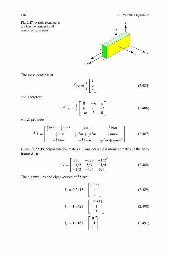
116 2 Vibration Dynamics
Fig. 2.27 A rigid rectangularbrick in the principal andnon-principal frames
The mass center is at
B ′rC = 1
2
⎡
⎣l
w
h
⎤
⎦ (2.485)
and, therefore,
B ′rC = 1
2
⎡
⎣0 −h w
h 0 −l
−w l 0
⎤
⎦ (2.486)
which provides
B ′I =
⎡
⎢⎣
13h2m + 1
3mw2 − 14 lmw − 1
4hlm
− 14 lmw 1
3h2m + 13 l2m − 1
4hmw
− 14hlm − 1
4hmw 13 l2m + 1
3mw2
⎤
⎥⎦ (2.487)
Example 72 (Principal rotation matrix) Consider a mass moment matrix in the bodyframe B1 as
1I =⎡
⎣2/3 −1/2 −1/2
−1/2 5/3 −1/4−1/2 −1/4 5/3
⎤
⎦ (2.488)
The eigenvalues and eigenvectors of 1I are
I1 = 0.2413
⎡
⎣2.351
11
⎤
⎦ (2.489)
I2 = 1.8421
⎡
⎣−0.851
11
⎤
⎦ (2.490)
I3 = 1.9167
⎡
⎣0
−11
⎤
⎦ (2.491)
2.3 Rigid Body Dynamics 117
The normalized eigenvector matrix W is the transpose of the required transforma-tion matrix to make the inertia matrix diagonal
W =⎡
⎣| | |
w1 w2 w3| | |
⎤
⎦ = 2RT1
=⎡
⎣0.856 9 −0.515 6 0.00.364 48 0.605 88 −0.707 110.364 48 0.605 88 0.707 11
⎤
⎦ (2.492)
We may verify that
2I = 2R11I 2RT
1 = WT1IW
=⎡
⎣0.2413 −1 × 10⁻⁴ 0.0
−1 × 10⁻⁴ 1.842 1 −1 × 10⁻¹⁹
0.0 0.0 1.916 7
⎤
⎦ (2.493)
Example 73 (� (Relative diagonal moments of inertia) By the definitions for themass moments (2.427), (2.428), and (2.429) it is seen that the inertia matrix is sym-metric, and
∫
B
(x2 + y2 + z2)dm = 1
2(Ixx + Iyy + Izz) (2.494)
and also
Ixx + Iyy ≥ Izz Iyy + Izz ≥ Ixx Izz + Ixx ≥ Iyy (2.495)
Noting that (y − z)2 ≥ 0, it is evident that (y2 + z2) ≥ 2yz, and therefore
Ixx ≥ 2Iyz (2.496)
and similarly
Iyy ≥ 2Izx Izz ≥ 2Ixy (2.497)
Example 74 � (Coefficients of the characteristic equation) The determinant(2.454)
∣∣∣∣∣∣
Ixx − λ Ixy Ixz
Iyx Iyy − λ Iyz
Izx Izy Izz − λ
∣∣∣∣∣∣= 0 (2.498)
for calculating the principal mass moments, leads to a third-degree equation for λ,called the characteristic equation:
λ3 − a1λ2 + a2λ − a3 = 0 (2.499)

118 2 Vibration Dynamics
The coefficients of the characteristic equation are called the principal invariantsof [I ]. The coefficients of the characteristic equation can directly be found from
a1 = Ixx + Iyy + Izz = tr [I ] (2.500)
a2 = IxxIyy + IyyIzz + IzzIxx − I 2xy − I 2
yz − I 2zx
=∣∣∣∣Ixx Ixy
Iyx Iyy
∣∣∣∣+∣∣∣∣Iyy Iyz
Izy Izz
∣∣∣∣+∣∣∣∣Ixx Ixz
Izx Izz
∣∣∣∣
= 1
2
(a2
1 − tr[I 2]) (2.501)
a3 = IxxIyyIzz + IxyIyzIzx + IzyIyxIxz
− (IxxIyzIzy + IyyIzxIxz + IzzIxyIyx)
= IxxIyyIzz + 2IxyIyzIzx − (IxxI
2yz + IyyI
2zx + IzzI
2xy
)
= det [I ] (2.502)
Example 75 � (The principal mass moments are coordinate invariants) The rootsof the inertia characteristic equation are the principal mass moments. They are allreal but not necessarily different. The principal mass moments are extreme. Thatis, the principal mass moments determine the smallest and the largest values of Iii .Since the smallest and largest values of Iii do not depend on the choice of the bodycoordinate frame, the solution of the characteristic equation is not dependent of thecoordinate frame.
In other words, if I1, I2, and I3 are the principal mass moments for B1I , theprincipal mass moments for B2I are also I1, I2, and I3 when
B2I = B2RB1B1IB2RT
B1
We conclude that I1, I2, and I3 are coordinate invariants of the matrix [I ], andtherefore any quantity that depends on I1, I2, and I3 is also coordinate invariant.Because the mass matrix [I ] has rank 3, it has only three independent invariants andevery other invariant can be expressed in terms of I1, I2, and I3.
Since I1, I2, and I3 are the solutions of the characteristic equation of [I ] given in(2.499), we may write the determinant (2.454) in the form
(λ − I1)(λ − I2)(λ − I3) = 0 (2.503)
The expanded form of this equation is
λ3 − (I1 + I2 + I3)λ2 + (I1I2 + I2I3 + I3I1)a2λ − I1I2I3 = 0 (2.504)
By comparing (2.504) and (2.499) we conclude that
a1 = Ixx + Iyy + Izz = I1 + I2 + I3 (2.505)
2.3 Rigid Body Dynamics 119
a2 = IxxIyy + IyyIzz + IzzIxx − I 2xy − I 2
yz − I 2zx
= I1I2 + I2I3 + I3I1 (2.506)
a3 = IxxIyyIzz + 2IxyIyzIzx − (IxxI
2yz + IyyI
2zx + IzzI
2xy
)
= I1I2I3 (2.507)
Being able to express the coefficients a1, a2, and a3 as functions of I1, I2, and I3, wedetermine the coefficients of the characteristic equation to be coordinate invariant.
Example 76 � (Short notation for the elements of inertia matrix) Taking advantageof the Kronecker delta δij (2.171) we may write the elements of the mass momentmatrix Iij in short:
Iij =∫
B
((x2
1 + x22 + x2
3
)δij − xixj
)dm (2.508)
Iij =∫
B
(r2δij − xixj
)dm (2.509)
Iij =∫
B
(3∑
k=1
xkxkδij − xixj
)dm (2.510)
where we utilized the following notation:
x1 = x x2 = y x3 = z (2.511)
Example 77 � (Mass moment with respect to a plane, a line, and a point) Themass moment of a system of particles may be defined with respect to a plane, a line,or a point as the sum of the products of the mass of the particles into the square ofthe perpendicular distance from the particle to the plane, the line, or the point. Fora continuous body, the sum would become a definite integral over the volume of thebody.
The mass moments with respect to the xy-, yz-, and zx-plane are
Iz2 =∫
B
z2 dm (2.512)
Iy2 =∫
B
y2 dm (2.513)
Ix2 =∫
B
x2 dm (2.514)
The moments of inertia with respect to the x, y, and z axes are
Ix =∫
B
(y2 + z2)dm (2.515)
120 2 Vibration Dynamics
Iy =∫
B
(z2 + x2)dm (2.516)
Iz =∫
B
(x2 + y2)dm (2.517)
and, therefore,
Ix = Iy2 + Iz2 (2.518)
Iy = Iz2 + Ix2 (2.519)
Iz = Ix2 + Iy2 (2.520)
The moment of inertia with respect to the origin is
Io =∫
B
(x2 + y2 + z2)dm = Ix2 + Iy2 + Iz2
= 1
2(Ix + Iy + Iz) (2.521)
Because the choice of the coordinate frame is arbitrary, the mass moment with re-spect to a line is the sum of the mass moments with respect to any two mutuallyorthogonal planes that pass through the line. The mass moment with respect to apoint has a similar meaning for three mutually orthogonal planes intersecting at thepoint.
2.4 Lagrange Method
The Lagrange method in deriving the equations of motion of vibrating systems hassome advantages over Newton–Euler due to its simplicity and generality, speciallyfor multi DOF systems.
2.4.1 � Lagrange Form of Newton Equation
Newton’s equation of motion can be transformed to
d
dt
(∂K
∂qr
)− ∂K
∂qr
= Fr r = 1,2, . . . , n (2.522)
where
Fr =n∑
i=1
(Fix
∂fi
∂q1+ Fiy
∂gi
∂q2+ Fiz
∂hi
∂qn
)(2.523)
2.4 Lagrange Method 121
Equation (2.522) is called the Lagrange equation of motion, where K is the kineticenergy of the n DOF system, qr , r = 1,2, . . . , n are the generalized coordinates ofthe system, Fi = [Fix Fiy Fiz]T is the external force acting on the ith particle of thesystem, and Fr is the generalized force associated to qr . The functions fi , gi , hi ,are the relationships of x1, yi , zi , based on the generalized coordinates of the systemxi = fi(qj , t), yi = gi(qj , t), zi = hi(qj , t).
Proof Let mi be the mass of one of the particles of a system and let (xi, yi, zi)
be its Cartesian coordinates in a globally fixed coordinate frame. Assume that thecoordinates of every individual particle are functions of another set of coordinatesq1, q2, q3, . . . , qn, and possibly time t :
xi = fi(q1, q2, q3, . . . , qn, t) (2.524)
yi = gi(q1, q2, q3, . . . , qn, t) (2.525)
zi = hi(q1, q2, q3, . . . , qn, t) (2.526)
If Fxi,Fyi,Fzi are components of the total force acting on the particle mi , thenthe Newton equations of motion for the particle would be
Fxi = mixi (2.527)
Fyi = miyi (2.528)
Fzi = mizi (2.529)
We multiply both sides of these equations by ∂fi/∂qr , ∂gi/∂qr , and ∂hi/∂qr , re-spectively, and add them up for all the particles to find
n∑
i=1
mi
(xi
∂fi
∂qr
+ yi
∂gi
∂qr
+ zi
∂hi
∂qr
)=
n∑
i=1
(Fxi
∂fi
∂qr
+ Fyi
∂gi
∂qr
+ Fzi
∂hi
∂qr
)(2.530)
where n is the total number of particles.Taking the time derivative of Eq. (2.524),
xi = ∂fi
∂q1q1 + ∂fi
∂q2q2 + ∂fi
∂q3q3 + · · · + ∂fi
∂qn
qn + ∂fi
∂t(2.531)
we find
∂xi
∂qr
= ∂
∂qr
(∂fi
∂q1q1 + ∂fi
∂q2q2 + · · · + ∂fi
∂qn
qn + ∂fi
∂t
)= ∂fi
∂qr
(2.532)
and, therefore,
xi
∂fi
∂qr
= xi
∂xi
∂qr
= d
dt
(xi
∂xi
∂qr
)− xi
d
dt
(∂xi
∂qr
)(2.533)
122 2 Vibration Dynamics
However,
xi
d
dt
(∂xi
∂qr
)= xi
d
dt
(∂fi
∂qr
)
= xi
(∂2fi
∂q1∂qr
q1 + · · · + ∂2fi
∂qn∂qr
qn + ∂2fi
∂t∂qr
)
= xi
∂
∂qr
(∂fi
∂q1q1 + ∂fi
∂q2q2 + · · · + ∂fi
∂qn
qn + ∂fi
∂t
)
= xi
∂xi
∂qr
(2.534)
and we have
xi
∂xi
∂qr
= d
dt
(xi
∂xi
∂qr
)− xi
∂xi
∂qr
(2.535)
which is equal to
xi
xi
qr
= d
dt
[∂
∂qr
(1
2x2i
)]− ∂
∂qr
(1
2x2i
)(2.536)
Now substituting (2.533) and (2.536) into the left-hand side of (2.530) yields
n∑
i=1
mi
(xi
∂fi
∂qr
+ yi
∂gi
∂qr
+ zi
∂hi
∂qr
)
=n∑
i=1
mi
d
dt
[∂
∂qr
(1
2x2i + 1
2y2i + 1
2z2i
)]
−n∑
i=1
mi
∂
∂qr
(1
2x2i + 1
2y2i + 1
2z2i
)
= 1
2
n∑
i=1
mi
d
dt
[∂
∂qr
(x2i + y2
i + z2i
)]
− 1
2
n∑
i=1
mi
∂
∂qr
(x2i + y2
i + z2i
)(2.537)
where
1
2
n∑
i=1
mi
(x2i + y2
i + z2i
) = K (2.538)
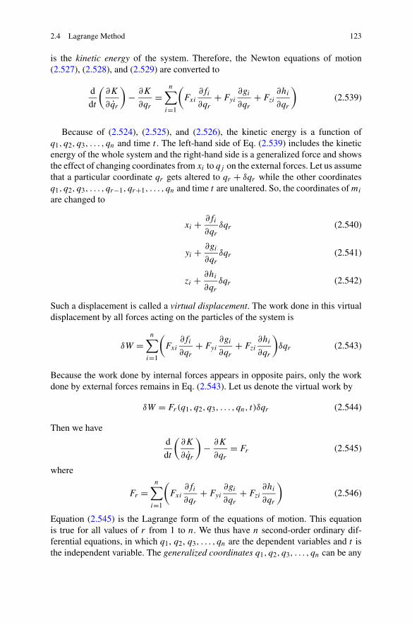
2.4 Lagrange Method 123
is the kinetic energy of the system. Therefore, the Newton equations of motion(2.527), (2.528), and (2.529) are converted to
d
dt
(∂K
∂qr
)− ∂K
∂qr
=n∑
i=1
(Fxi
∂fi
∂qr
+ Fyi
∂gi
∂qr
+ Fzi
∂hi
∂qr
)(2.539)
Because of (2.524), (2.525), and (2.526), the kinetic energy is a function ofq1, q2, q3, . . . , qn and time t . The left-hand side of Eq. (2.539) includes the kineticenergy of the whole system and the right-hand side is a generalized force and showsthe effect of changing coordinates from xi to qj on the external forces. Let us assumethat a particular coordinate qr gets altered to qr + δqr while the other coordinatesq1, q2, q3, . . . , qr−1, qr+1, . . . , qn and time t are unaltered. So, the coordinates of mi
are changed to
xi + ∂fi
∂qr
δqr (2.540)
yi + ∂gi
∂qr
δqr (2.541)
zi + ∂hi
∂qr
δqr (2.542)
Such a displacement is called a virtual displacement. The work done in this virtualdisplacement by all forces acting on the particles of the system is
δW =n∑
i=1
(Fxi
∂fi
∂qr
+ Fyi
∂gi
∂qr
+ Fzi
∂hi
∂qr
)δqr (2.543)
Because the work done by internal forces appears in opposite pairs, only the workdone by external forces remains in Eq. (2.543). Let us denote the virtual work by
δW = Fr(q1, q2, q3, . . . , qn, t)δqr (2.544)
Then we have
d
dt
(∂K
∂qr
)− ∂K
∂qr
= Fr (2.545)
where
Fr =n∑
i=1
(Fxi
∂fi
∂qr
+ Fyi
∂gi
∂qr
+ Fzi
∂hi
∂qr
)(2.546)
Equation (2.545) is the Lagrange form of the equations of motion. This equationis true for all values of r from 1 to n. We thus have n second-order ordinary dif-ferential equations, in which q1, q2, q3, . . . , qn are the dependent variables and t isthe independent variable. The generalized coordinates q1, q2, q3, . . . , qn can be any
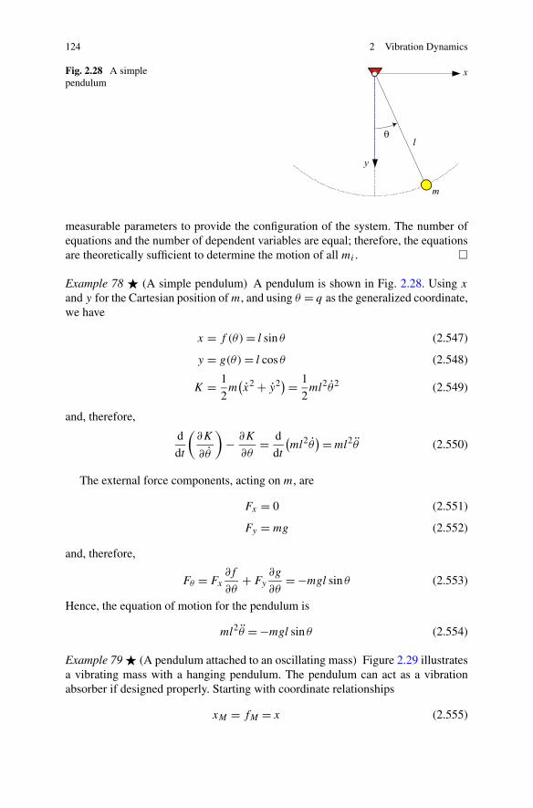
124 2 Vibration Dynamics
Fig. 2.28 A simplependulum
measurable parameters to provide the configuration of the system. The number ofequations and the number of dependent variables are equal; therefore, the equationsare theoretically sufficient to determine the motion of all mi . �
Example 78 � (A simple pendulum) A pendulum is shown in Fig. 2.28. Using x
and y for the Cartesian position of m, and using θ = q as the generalized coordinate,we have
x = f (θ) = l sin θ (2.547)
y = g(θ) = l cos θ (2.548)
K = 1
2m(x2 + y2) = 1
2ml2θ2 (2.549)
and, therefore,
d
dt
(∂K
∂θ
)− ∂K
∂θ= d
dt
(ml2θ
) = ml2θ (2.550)
The external force components, acting on m, are
Fx = 0 (2.551)
Fy = mg (2.552)
and, therefore,
Fθ = Fx
∂f
∂θ+ Fy
∂g
∂θ= −mgl sin θ (2.553)
Hence, the equation of motion for the pendulum is
ml2θ = −mgl sin θ (2.554)
Example 79 � (A pendulum attached to an oscillating mass) Figure 2.29 illustratesa vibrating mass with a hanging pendulum. The pendulum can act as a vibrationabsorber if designed properly. Starting with coordinate relationships
xM = fM = x (2.555)
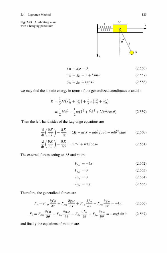
2.4 Lagrange Method 125
Fig. 2.29 A vibrating masswith a hanging pendulum
yM = gM = 0 (2.556)
xm = fm = x + l sin θ (2.557)
ym = gm = l cos θ (2.558)
we may find the kinetic energy in terms of the generalized coordinates x and θ :
K = 1
2M
(x2M + y2
M
)+ 1
2m(x2m + y2
m
)
= 1
2Mx2 + 1
2m(x2 + l2θ2 + 2lxθ cos θ
)(2.559)
Then the left-hand sides of the Lagrange equations are
d
dt
(∂K
∂x
)− ∂K
∂x= (M + m)x + mlθ cos θ − mlθ2 sin θ (2.560)
d
dt
(∂K
∂θ
)− ∂K
∂θ= ml2θ + mlx cos θ (2.561)
The external forces acting on M and m are
FxM= −kx (2.562)
FyM= 0 (2.563)
Fxm = 0 (2.564)
Fym = mg (2.565)
Therefore, the generalized forces are
Fx = FxM
∂fM
∂x+ FyM
∂gM
∂x+ Fxm
∂fm
∂x+ Fym
∂gm
∂x= −kx (2.566)
Fθ = FxM
∂fM
∂θ+ FyM
∂gM
∂θ+ Fxm
∂fm
∂θ+ Fym
∂gm
∂θ= −mgl sin θ (2.567)
and finally the equations of motion are

126 2 Vibration Dynamics
(M + m)x + mlθ cos θ − mlθ2 sin θ = −kx (2.568)
ml2θ + mlx cos θ = −mgl sin θ (2.569)
2.4.2 Lagrangean Mechanics
Let us assume that for some forces F = [Fix Fiy Fiz]T there is a function V , calledpotential energy, such that the force is derivable from V
F = −∇V (2.570)
Such a force is called a potential or conservative force. Then the Lagrange equationof motion can be written as
d
dt
(∂L∂qr
)− ∂L
∂qr
= Qr r = 1,2, . . . , n (2.571)
where
L = K − V (2.572)
is the Lagrangean of the system and Qr is the nonpotential generalized force
Qr =n∑
i=1
(Fix
∂fi
∂q1+ Fiy
∂gi
∂q2+ Fiz
∂hi
∂qn
)(2.573)
for which there is no potential function.
Proof Assume that the external forces F = [Fxi Fyi Fzi]T acting on the system areconservative:
F = −∇V (2.574)
The work done by these forces in an arbitrary virtual displacement δq1, δq2,δq3, . . . , δqn is
∂W = − ∂V
∂q1δq1 − ∂V
∂q2δq2 − · · · ∂V
∂qn
δqn (2.575)
and then the Lagrange equation becomes
d
dt
(∂K
∂qr
)− ∂K
∂qr
= − ∂V
∂q1r = 1,2, . . . , n (2.576)
Introducing the Lagrangean function L = K −V converts the Lagrange equation ofa conservative system to
d
dt
(∂L∂qr
)− ∂L
∂qr
= 0 r = 1,2, . . . , n (2.577)
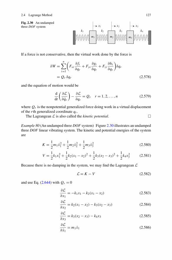
2.4 Lagrange Method 127
Fig. 2.30 An undampedthree DOF system
If a force is not conservative, then the virtual work done by the force is
δW =n∑
i=1
(Fxi
∂fi
∂qr
+ Fyi
∂gi
∂qr
+ Fzi
∂hi
∂qr
)δqr
= Qr δqr (2.578)
and the equation of motion would be
d
dt
(∂L∂qr
)− ∂L
∂qr
= Qr r = 1,2, . . . , n (2.579)
where Qr is the nonpotential generalized force doing work in a virtual displacementof the r th generalized coordinate qr .
The Lagrangean L is also called the kinetic potential. �
Example 80 (An undamped three DOF system) Figure 2.30 illustrates an undampedthree DOF linear vibrating system. The kinetic and potential energies of the systemare
K = 1
2m1x
21 + 1
2m2x
22 + 1
2m3x
23 (2.580)
V = 1
2k1x
21 + 1
2k2(x1 − x2)
2 + 1
2k3(x2 − x3)
2 + 1
2k4x
23 (2.581)
Because there is no damping in the system, we may find the Lagrangean L
L = K − V (2.582)
and use Eq. (2.644) with Qr = 0
∂L∂x1
= −k1x1 − k2(x1 − x2) (2.583)
∂L∂x2
= k2(x1 − x2) − k3(x2 − x3) (2.584)
∂L∂x3
= k3(x2 − x3) − k4x3 (2.585)
∂L∂x1
= m1x1 (2.586)
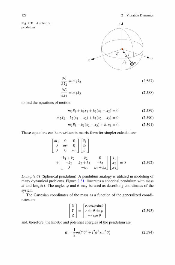
128 2 Vibration Dynamics
Fig. 2.31 A sphericalpendulum
∂L∂x2
= m2x2 (2.587)
∂L∂x3
= m3x3 (2.588)
to find the equations of motion:
m1x1 + k1x1 + k2(x1 − x2) = 0 (2.589)
m2x2 − k2(x1 − x2) + k3(x2 − x3) = 0 (2.590)
m3x3 − k3(x2 − x3) + k4x3 = 0 (2.591)
These equations can be rewritten in matrix form for simpler calculation:⎡
⎣m1 0 00 m2 00 0 m3
⎤
⎦
⎡
⎣x1x2x3
⎤
⎦
+⎡
⎣k1 + k2 −k2 0−k2 k2 + k3 −k3
0 −k3 k3 + k4
⎤
⎦
⎡
⎣x1x2x3
⎤
⎦ = 0 (2.592)
Example 81 (Spherical pendulum) A pendulum analogy is utilized in modeling ofmany dynamical problems. Figure 2.31 illustrates a spherical pendulum with massm and length l. The angles ϕ and θ may be used as describing coordinates of thesystem.
The Cartesian coordinates of the mass as a function of the generalized coordi-nates are
⎡
⎣X
Y
Z
⎤
⎦ =⎡
⎣r cosϕ sin θ
r sin θ sinϕ
−r cos θ
⎤
⎦ (2.593)
and, therefore, the kinetic and potential energies of the pendulum are
K = 1
2m(l2θ2 + l2ϕ2 sin2 θ
)(2.594)

2.4 Lagrange Method 129
Fig. 2.32 A controlledcompound pendulum
V = −mgl cos θ (2.595)
The kinetic potential function of this system is
L = 1
2m(l2θ2 + l2ϕ2 sin2 θ
)+ mgl cos θ (2.596)
which leads to the following equations of motion:
θ − ϕ2 sin θ cos θ + g
lsin θ = 0 (2.597)
ϕ sin2 θ + 2ϕθ sin θ cos θ = 0 (2.598)
Example 82 (Controlled compound pendulum) A massive arm is attached to a ceil-ing at a pin joint O as illustrated in Fig. 2.32. Assume that there is viscous frictionin the joint where an ideal motor can apply a torque Q to move the arm. The rotorof an ideal motor has no mass moment by assumption.
The kinetic and potential energies of the manipulator are
K = 1
2I θ2 = 1
2
(IC + ml2)θ2 (2.599)
V = −mg cos θ (2.600)
where m is the mass and I is the mass moment of the pendulum about O . TheLagrangean of the manipulator is
L = K − V = 1
2I θ2 + mg cos θ (2.601)
and, therefore, the equation of motion of the pendulum is
M = d
dt
(∂L∂θ
)− ∂L
∂θ= I θ + mgl sin θ (2.602)
The generalized force M is the contribution of the motor torque Q and the vis-cous friction torque −cθ . Hence, the equation of motion of the manipulator is
Q = I θ + cθ + mgl sin θ (2.603)
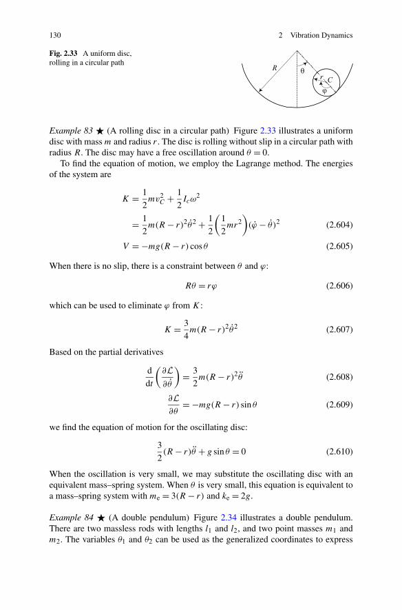
130 2 Vibration Dynamics
Fig. 2.33 A uniform disc,rolling in a circular path
Example 83 � (A rolling disc in a circular path) Figure 2.33 illustrates a uniformdisc with mass m and radius r . The disc is rolling without slip in a circular path withradius R. The disc may have a free oscillation around θ = 0.
To find the equation of motion, we employ the Lagrange method. The energiesof the system are
K = 1
2mv2
C + 1
2Icω
2
= 1
2m(R − r)2θ2 + 1
2
(1
2mr2
)(ϕ − θ )2 (2.604)
V = −mg(R − r) cos θ (2.605)
When there is no slip, there is a constraint between θ and ϕ:
Rθ = rϕ (2.606)
which can be used to eliminate ϕ from K :
K = 3
4m(R − r)2θ2 (2.607)
Based on the partial derivatives
d
dt
(∂L∂θ
)= 3
2m(R − r)2θ (2.608)
∂L∂θ
= −mg(R − r) sin θ (2.609)
we find the equation of motion for the oscillating disc:
3
2(R − r)θ + g sin θ = 0 (2.610)
When the oscillation is very small, we may substitute the oscillating disc with anequivalent mass–spring system. When θ is very small, this equation is equivalent toa mass–spring system with me = 3(R − r) and ke = 2g.
Example 84 � (A double pendulum) Figure 2.34 illustrates a double pendulum.There are two massless rods with lengths l1 and l2, and two point masses m1 andm2. The variables θ1 and θ2 can be used as the generalized coordinates to express
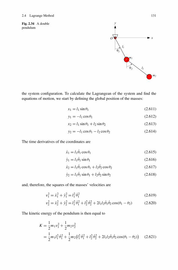
2.4 Lagrange Method 131
Fig. 2.34 A doublependulum
the system configuration. To calculate the Lagrangean of the system and find theequations of motion, we start by defining the global position of the masses:
x1 = l1 sin θ1 (2.611)
y1 = −l1 cos θ1 (2.612)
x2 = l1 sin θ1 + l2 sin θ2 (2.613)
y2 = −l1 cos θ1 − l2 cos θ2 (2.614)
The time derivatives of the coordinates are
x1 = l1θ1 cos θ1 (2.615)
y1 = l1θ1 sin θ1 (2.616)
x2 = l1θ1 cos θ1 + l2θ2 cos θ2 (2.617)
y2 = l1θ1 sin θ1 + l2θ2 sin θ2 (2.618)
and, therefore, the squares of the masses’ velocities are
v21 = x2
1 + y21 = l2
1 θ21 (2.619)
v22 = x2
2 + y22 = l2
1 θ21 + l2
2 θ22 + 2l1l2θ1θ2 cos(θ1 − θ2) (2.620)
The kinetic energy of the pendulum is then equal to
K = 1
2m1v
21 + 1
2m2v
22
= 1
2m1l
21 θ2
1 + 1
2m2
(l21 θ2
1 + l22 θ2
2 + 2l1l2θ1θ2 cos(θ1 − θ2))
(2.621)
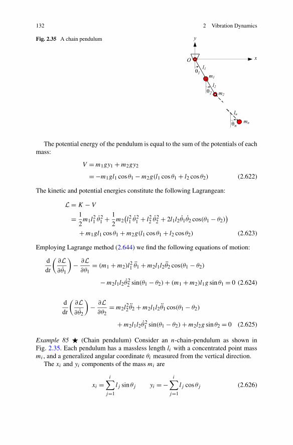
132 2 Vibration Dynamics
Fig. 2.35 A chain pendulum
The potential energy of the pendulum is equal to the sum of the potentials of eachmass:
V = m1gy1 + m2gy2
= −m1gl1 cos θ1 − m2g(l1 cos θ1 + l2 cos θ2) (2.622)
The kinetic and potential energies constitute the following Lagrangean:
L = K − V
= 1
2m1l
21 θ2
1 + 1
2m2
(l21 θ2
1 + l22 θ2
2 + 2l1l2θ1θ2 cos(θ1 − θ2))
+ m1gl1 cos θ1 + m2g(l1 cos θ1 + l2 cos θ2) (2.623)
Employing Lagrange method (2.644) we find the following equations of motion:
d
dt
(∂L∂θ1
)− ∂L
∂θ1= (m1 + m2)l
21 θ1 + m2l1l2θ2 cos(θ1 − θ2)
− m2l1l2θ22 sin(θ1 − θ2) + (m1 + m2)l1g sin θ1 = 0 (2.624)
d
dt
(∂L∂θ2
)− ∂L
∂θ2= m2l
22 θ2 + m2l1l2θ1 cos(θ1 − θ2)
+ m2l1l2θ21 sin(θ1 − θ2) + m2l2g sin θ2 = 0 (2.625)
Example 85 � (Chain pendulum) Consider an n-chain-pendulum as shown inFig. 2.35. Each pendulum has a massless length li with a concentrated point massmi , and a generalized angular coordinate θi measured from the vertical direction.
The xi and yi components of the mass mi are
xi =i∑
j=1
lj sin θj yi = −i∑
j=1
lj cos θj (2.626)

2.4 Lagrange Method 133
We find their time derivatives:
xi =i∑
j=1
lj θj cos θj yi =i∑
j=1
lj θj sin θj (2.627)
and the square of xi and yi :
x2i =
(i∑
j=1
lj θj cos θj
)(i∑
k=1
lk θk cos θk
)=
n∑
j=1
n∑
k=1
lj lkθj θk cos θj cos θk (2.628)
y2i =
(i∑
j=1
lj θj sin θj
)(i∑
k=1
lk θk sin θk
)=
i∑
j=1
i∑
k=1
lj lkθj θk sin θj sin θk (2.629)
to calculate the velocity vi of the mass mi :
v2i = x2
i + y2i
=i∑
j=1
i∑
k=1
lj lkθj θk(cos θj cos θk + sin θj sin θk)
=i∑
j=1
i∑
k=1
lj lkθj θk cos(θj − θk)
=i∑
r=1
l2r θ2
r + 2i∑
j=1
i∑
k=j+1
lj lkθj θk cos(θj − θk) (2.630)
Now, we calculate the kinetic energy, K , of the chain:
K = 1
2
n∑
i=1
miv2i
= 1
2
n∑
i=1
mi
(i∑
r=1
l2r θ2
r + 2i∑
j=1
i∑
k=j+1
lj lkθj θk cos(θj − θk)
)
= 1
2
n∑
i=1
i∑
r=1
mil2r θ
2r +
n∑
i=1
i∑
j=1
i∑
k=j+1
milj lkθj θk cos(θj − θk) (2.631)
The potential energy of the ith pendulum is related to mi ,
Vi = migyi = −mig
i∑
j=1
lj cos θj (2.632)

134 2 Vibration Dynamics
and, therefore, the potential energy of the chain is
V =n∑
i=1
migyi = −n∑
i=1
i∑
j=1
miglj cos θj (2.633)
To find the equations of motion for the chain, we may use the Lagrangean L
L = K − V (2.634)
and apply the Lagrange equation
d
dt
(∂L∂qs
)− ∂L
∂qs
= 0 s = 1,2, . . . , n (2.635)
or
d
dt
(∂K
∂qs
)− ∂K
∂qs
+ ∂V
∂qs
= 0 s = 1,2, . . . , n (2.636)
Example 86 (Mechanical energy) If a system of masses mi are moving in a poten-tial force field
Fmi= −∇iV (2.637)
their Newton equations of motion will be
mi ri = −∇iV i = 1,2, . . . , n (2.638)
The inner product of equations of motion with ri and adding the equations
n∑
i=1
mi ri · ri = −n∑
i=1
ri · ∇iV (2.639)
and then integrating over time
1
2
n∑
i=1
mi ri · ri = −∫ n∑
i=1
ri · ∇iV (2.640)
shows that
K = −∫ n∑
i=1
(∂V
∂xi
xi + ∂V
∂yi
yi + ∂V
∂zi
zi
)= −V + E (2.641)
where E is the constant of integration. E is called the mechanical energy of thesystem and is equal to kinetic plus potential energies:
E = K + V (2.642)

2.5 Dissipation Function 135
2.5 Dissipation Function
The Lagrange equation,
d
dt
(∂K
∂qr
)− ∂K
∂qr
= Fr r = 1,2, . . . , n (2.643)
or
d
dt
(∂L∂qr
)− ∂L
∂qr
= Qr r = 1,2, . . . , n (2.644)
as introduced in Eqs. (2.522) and (2.571) can both be applied to find the equationsof motion of a vibrating system. However, for small and linear vibrations, we mayuse a simpler and more practical Lagrange equation, thus:
d
dt
(∂K
∂qr
)− ∂K
∂qr
+ ∂D
∂qr
+ ∂V
∂qr
= fr r = 1,2, . . . , n (2.645)
where K is the kinetic energy, V is the potential energy, and D is the dissipationfunction of the system
K = 1
2qT[m]q = 1
2
n∑
i=1
n∑
j=1
qimij qj (2.646)
V = 1
2qT[k]q = 1
2
n∑
i=1
n∑
j=1
qikij qj (2.647)
D = 1
2qT[c]q = 1
2
n∑
i=1
n∑
j=1
qicij qj (2.648)
and fr is the applied force on the mass mr .
Proof Consider a one DOF mass–spring–damper vibrating system. When viscousdamping is the only type of damping in the system, we may employ a functionknown as the Rayleigh dissipation function
D = 1
2cx2 (2.649)
to find the damping force fc by differentiation:
fc = −∂D
∂x(2.650)
Remembering that the elastic force fk can be found from a potential energy V
fk = −∂V
∂x(2.651)
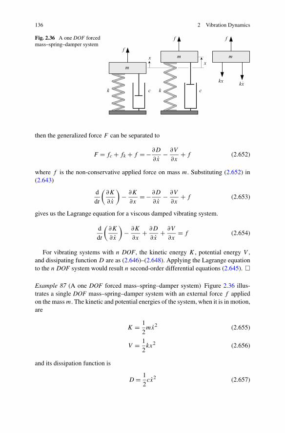
136 2 Vibration Dynamics
Fig. 2.36 A one DOF forcedmass–spring–damper system
then the generalized force F can be separated to
F = fc + fk + f = −∂D
∂x− ∂V
∂x+ f (2.652)
where f is the non-conservative applied force on mass m. Substituting (2.652) in(2.643)
d
dt
(∂K
∂x
)− ∂K
∂x= −∂D
∂x− ∂V
∂x+ f (2.653)
gives us the Lagrange equation for a viscous damped vibrating system.
d
dt
(∂K
∂x
)− ∂K
∂x+ ∂D
∂x+ ∂V
∂x= f (2.654)
For vibrating systems with n DOF, the kinetic energy K , potential energy V ,and dissipating function D are as (2.646)–(2.648). Applying the Lagrange equationto the n DOF system would result n second-order differential equations (2.645). �
Example 87 (A one DOF forced mass–spring–damper system) Figure 2.36 illus-trates a single DOF mass–spring–damper system with an external force f appliedon the mass m. The kinetic and potential energies of the system, when it is in motion,are
K = 1
2mx2 (2.655)
V = 1
2kx2 (2.656)
and its dissipation function is
D = 1
2cx2 (2.657)
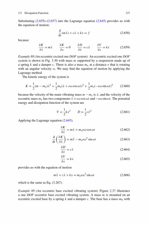
2.5 Dissipation Function 137
Substituting (2.655)–(2.657) into the Lagrange equation (2.645) provides us withthe equation of motion:
d
dt(mx) + cx + kx = f (2.658)
because
∂K
∂x= mx
∂K
∂x= 0
∂D
∂x= cx
∂V
∂x= kx (2.659)
Example 88 (An eccentric excited one DOF system) An eccentric excited one DOFsystem is shown in Fig. 3.30 with mass m supported by a suspension made up ofa spring k and a damper c. There is also a mass me at a distance e that is rotatingwith an angular velocity ω. We may find the equation of motion by applying theLagrange method.
The kinetic energy of the system is
K = 1
2(m − me)x
2 + 1
2me(x + eω cosωt)2 + 1
2me(−eω sinωt)2 (2.660)
because the velocity of the main vibrating mass m− me is x, and the velocity of theeccentric mass me has two components x + eω cosωt and −eω sinωt . The potentialenergy and dissipation function of the system are
V = 1
2kx2 D = 1
2cx2 (2.661)
Applying the Lagrange equation (2.645),
∂K
∂x= mx + meeω cosωt (2.662)
d
dt
(∂K
∂x
)= mx − meeω
2 sinωt (2.663)
∂D
∂x= cx (2.664)
∂V
∂x= kx (2.665)
provides us with the equation of motion
mx + cx + kx = meeω2 sinωt (2.666)
which is the same as Eq. (3.267).
Example 89 (An eccentric base excited vibrating system) Figure 2.37 illustratesa one DOF eccentric base excited vibrating system. A mass m is mounted on aneccentric excited base by a spring k and a damper c. The base has a mass mb with

138 2 Vibration Dynamics
Fig. 2.37 A one DOFeccentric base excitedvibrating system
an attached unbalance mass me at a distance e. The mass me is rotating with anangular velocity ω.
We may derive the equation of motion of the system by applying Lagrangemethod. The required functions are
K = 1
2mx2 + 1
2(mb − me)y
2
+ 1
2me(y − eω cosωt)2 + 1
2me(eω sinωt)2 (2.667)
V = 1
2k(x − y)2 (2.668)
D = 1
2c(x − y)2 (2.669)
Applying the Lagrange method (2.645) provides us with the equations
mx + c(x − y) + k(x − y) = 0 (2.670)
mby + meeω2 sinωt − c(x − y) − k(x − y) = 0 (2.671)
because
∂K
∂x= mx (2.672)
d
dt
(∂K
∂x
)= mx (2.673)
∂D
∂x= c(x − y) (2.674)
∂V
∂x= k(x − y) (2.675)
∂K
∂y= mby − meeω cosωt (2.676)
d
dt
(∂K
∂y
)= mby + meeω
2 sinωt (2.677)
2.5 Dissipation Function 139
∂D
∂y= −c(x − y) (2.678)
∂V
∂y= −k(x − y) (2.679)
Using z = x − y, we may combine Eqs. (2.670) and (2.671) to find the equation ofrelative motion
mmb
mb + mz + cz + kz = mme
mb + meω2 sinωt (2.680)
which is equal to
z + 2ξωn z + ω2n z = εeω2 sinωt (2.681)
ε = me
mb(2.682)
Example 90 � (Generalized forces)1. Elastic force:An elastic force is a recoverable force from an elastic body that has changed its
internal energy. An elastic body is a body for which any produced work is stored inthe body in the form of internal energy, and is recoverable. Therefore, the variationof the internal potential energy of the body, V = V (q, t) would be
δV = −δW =n∑
i=1
Qiδqi (2.683)
where qi is the generalized coordinate of the particle i of the body, δW is the virtualwork of the generalized elastic force Q:
Qi = − ∂V
∂qi
(2.684)
2. Dissipation force:A dissipative force between two bodies is proportional to and in opposite direc-
tion of the relative velocity vector v between two bodies:
Qi = −cifi(vi)vi
vi
(2.685)
The coefficient ci is a constant, fi(vi) is the velocity function of the force, and vi
is the magnitude of the relative velocity:
vi =
√√√√√3∑
j=1
v2ij (2.686)
140 2 Vibration Dynamics
The virtual work of the dissipation force is
δW =n1∑
i=1
Qiδqi (2.687)
Qi = −n1∑
k=1
ckfk(vk)∂vk
∂qi
(2.688)
where n1 is the total number of dissipation forces. By introducing the dissipationfunction D as
D =n1∑
i=1
∫ vi
0ckfk(zk)dz (2.689)
we have
Qi = −∂D
∂qi
(2.690)
The dissipation power P of the dissipation force Qi is
P =n∑
i=1
Qiqi =n∑
i=1
qi
∂D
∂qi
(2.691)
2.6 � Quadratures
If [m] is an n × n square matrix and x is an n × 1 vector, then S is a scalar functioncalled quadrature and is defined by
S = xT[m]x (2.692)
The derivative of the quadrature S with respect to the vector x is
∂S
∂x= ([m] + [m]T)x (2.693)
Kinetic energy K , potential energy V , and dissipation function D are quadratures
K = 1
2xT[m]x (2.694)
V = 1
2xT[k]x (2.695)
D = 1
2xT[c]x (2.696)

2.6 Quadratures 141
and, therefore,
∂K
∂ x= 1
2
([m] + [m]T)x (2.697)
∂V
∂x= 1
2
([k] + [k]T)x (2.698)
∂D
∂ x= 1
2
([c] + [c]T)x (2.699)
Employing quadrature derivatives and the Lagrange method,
d
dt
∂K
∂ x+ ∂K
∂x+ ∂D
∂ x+ ∂V
∂x= F (2.700)
δW = FT∂x (2.701)
the equation of motion for a linear n degree-of-freedom vibrating system becomes
[m]x + [c]x + [k]x = F (2.702)
where [m], [c], [k] are symmetric matrices:
[m] = 1
2
([m] + [m]T) (2.703)
[c] = 1
2
([c] + [c]T) (2.704)
[k] = 1
2
([k] + [k]T) (2.705)
Quadratures are also called Hermitian forms.
Proof Let us define a general asymmetric quadrature as
S = xT[a]y =∑
i
∑
j
xiaij yj (2.706)
If the quadrature is symmetric, then x = y and
S = xT[a]x =∑
i
∑
j
xiaij xj (2.707)
The vectors x and y may be functions of n generalized coordinates qi and time t :
x = x(q1, q2, . . . , qn, t) (2.708)
y = y(q1, q2, . . . , qn, t) (2.709)
q = [q1 q2 · · · qn
]T (2.710)

142 2 Vibration Dynamics
The derivative of x with respect to q is a square matrix
∂x∂q
=
⎡
⎢⎢⎢⎢⎣
∂x1∂q1
∂x2∂q1
· · · ∂xn
∂q1∂x1∂q2
∂x2∂q2
· · · . . .
. . . · · · . . . · · ·∂x1∂qn
· · · · · · ∂xn
∂qn
⎤
⎥⎥⎥⎥⎦(2.711)
which can also be expressed by
∂x∂q
=
⎡
⎢⎢⎢⎢⎣
∂x∂q1∂x∂q2
. . .
∂x∂qn
⎤
⎥⎥⎥⎥⎦(2.712)
or
∂x∂q
=[
∂x1∂q
∂x2∂q . . . ∂xn
∂q
](2.713)
The derivative of S with respect to an element of qk is
∂S
∂qk
= ∂
∂qk
∑
i
∑
j
xiaij yj
=∑
i
∑
j
∂xi
∂qk
aij yj +∑
i
∑
j
xiaij
∂yj
∂qk
=∑
j
∑
i
∂xi
∂qk
aij yj +∑
i
∑
j
∂yj
∂qk
aij xi
=∑
j
∑
i
∂xi
∂qk
aij yj +∑
j
∑
i
∂yi
∂qk
ajixj (2.714)
and, hence, the derivative of S with respect to q is
∂S
∂q= ∂x
∂q[a]y + ∂y
∂q[a]Tx (2.715)
If S is a symmetric quadrature, then
∂S
∂q= ∂
∂q
(xT[a]x) = ∂x
∂q[a]x + ∂x
∂q[a]Tx (2.716)

2.6 Quadratures 143
and if q = x, then the derivative of a symmetric S with respect to x is
∂S
∂x= ∂
∂x
(xT[a]x) = ∂x
∂x[a]x + ∂x
∂x[a]Tx
= [a]x + [a]Tx = ([a] + [a]T)x (2.717)
If [a] is a symmetric matrix, then
[a] + [a]T = 2[a] (2.718)
however, if [a] is not a symmetric matrix, then [a] = [a] + [a]T is a symmetricmatrix because
aij = aij + aji = aji + aij = aji (2.719)
and, therefore,
[a] = [a]T (2.720)
Kinetic energy K , potential energy V , and dissipation function D can be ex-pressed by quadratures:
K = 1
2xT[m]x (2.721)
V = 1
2xT[k]x (2.722)
D = 1
2xT[c]x (2.723)
Substituting K , V , and D in the Lagrange equation provides us with the equationsof motion:
F = d
dt
∂K
∂ x+ ∂K
∂x+ ∂D
∂ x+ ∂V
∂x
= 1
2
d
dt
∂
∂ x
(xT[m]x)+ 1
2
∂
∂ x
(xT[c]x)+ 1
2
∂
∂x
(xT[k]x)
= 1
2
[d
dt
(([m] + [m]T)x)+ ([c] + [c]T)x + ([k] + [k]T)x
]
= 1
2
([m] + [m]T)x + 1
2
([c] + [c]T) ˙x+1
2
([k] + [k]T)x
= [m]x + [c]x + [k]x (2.724)
where
[m] = 1
2
([m] + [m]T) (2.725)
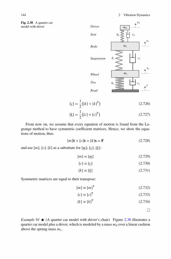
144 2 Vibration Dynamics
Fig. 2.38 A quarter carmodel with driver
[c] = 1
2
([k] + [k]T) (2.726)
[k] = 1
2
([c] + [c]T) (2.727)
From now on, we assume that every equation of motion is found from the La-grange method to have symmetric coefficient matrices. Hence, we show the equa-tions of motion, thus:
[m]x + [c]x + [k]x = F (2.728)
and use [m], [c], [k] as a substitute for [m], [c], [k]:[m] ≡ [m] (2.729)
[c] ≡ [c] (2.730)
[k] ≡ [k] (2.731)
Symmetric matrices are equal to their transpose:
[m] ≡ [m]T (2.732)
[c] ≡ [c]T (2.733)
[k] ≡ [k]T (2.734)
�
Example 91 � (A quarter car model with driver’s chair) Figure 2.38 illustrates aquarter car model plus a driver, which is modeled by a mass md over a linear cushionabove the sprung mass ms.
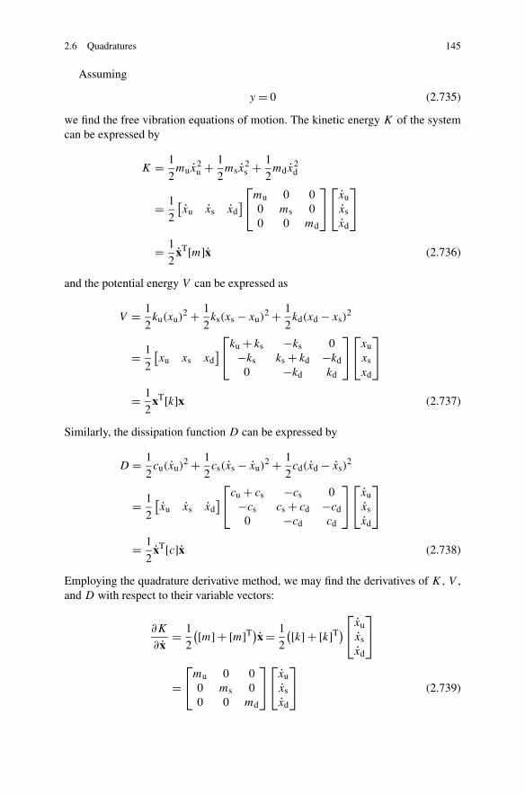
2.6 Quadratures 145
Assuming
y = 0 (2.735)
we find the free vibration equations of motion. The kinetic energy K of the systemcan be expressed by
K = 1
2mux
2u + 1
2msx
2s + 1
2mdx
2d
= 1
2
[xu xs xd
]⎡
⎣mu 0 00 ms 00 0 md
⎤
⎦
⎡
⎣xuxsxd
⎤
⎦
= 1
2xT[m]x (2.736)
and the potential energy V can be expressed as
V = 1
2ku(xu)
2 + 1
2ks(xs − xu)
2 + 1
2kd(xd − xs)
2
= 1
2
[xu xs xd
]⎡
⎣ku + ks −ks 0−ks ks + kd −kd
0 −kd kd
⎤
⎦
⎡
⎣xuxsxd
⎤
⎦
= 1
2xT[k]x (2.737)
Similarly, the dissipation function D can be expressed by
D = 1
2cu(xu)
2 + 1
2cs(xs − xu)
2 + 1
2cd(xd − xs)
2
= 1
2
[xu xs xd
]⎡
⎣cu + cs −cs 0−cs cs + cd −cd
0 −cd cd
⎤
⎦
⎡
⎣xuxsxd
⎤
⎦
= 1
2xT[c]x (2.738)
Employing the quadrature derivative method, we may find the derivatives of K , V ,and D with respect to their variable vectors:
∂K
∂ x= 1
2
([m] + [m]T)x = 1
2
([k] + [k]T)⎡
⎣xuxsxd
⎤
⎦
=⎡
⎣mu 0 00 ms 00 0 md
⎤
⎦
⎡
⎣xuxsxd
⎤
⎦ (2.739)

146 2 Vibration Dynamics
∂V
∂x= 1
2
([k] + [k]T)x = 1
2
([k] + [k]T)⎡
⎣xuxsxd
⎤
⎦
=⎡
⎣ku + ks −ks 0−ks ks + kd −kd
0 −kd kd
⎤
⎦
⎡
⎣xuxsxd
⎤
⎦ (2.740)
∂D
∂ x= 1
2
([c] + [c]T)x
= 1
2
([c] + [c]T)⎡
⎣xuxsxd
⎤
⎦
=⎡
⎣cu + cs −cs 0−cs cs + cd −cd
0 −cd cd
⎤
⎦
⎡
⎣xuxsxd
⎤
⎦ (2.741)
Therefore, we find the system’s free vibration equations of motion:
[m]x + [c]x + [k]x = 0 (2.742)
⎡
⎣mu 0 00 ms 00 0 md
⎤
⎦
⎡
⎣xuxsxd
⎤
⎦+⎡
⎣cu + cs −cs 0−cs cs + cd −cd
0 −cd cd
⎤
⎦
⎡
⎣xuxsxd
⎤
⎦
+⎡
⎣ku + ks −ks 0−ks ks + kd −kd
0 −kd kd
⎤
⎦
⎡
⎣xuxsxd
⎤
⎦ = 0 (2.743)
Example 92 � (Different [m], [c], and [k] arrangements) Mass, damping, and stiff-ness matrices [m], [c], [k] for a vibrating system may be arranged in different formswith the same overall kinetic energy K , potential energy V , and dissipation functionD. For example, the potential energy V for the quarter car model that is shown inFig. 2.38 may be expressed by different [k]:
V = 1
2ku(xu)
2 + 1
2ks(xs − xu)
2 + 1
2kd(xd − xs)
2 (2.744)
V = 1
2xT
⎡
⎣ku + ks −ks 0−ks ks + kd −kd
0 −kd kd
⎤
⎦x (2.745)
V = 1
2xT
⎡
⎣ku + ks −2ks 0
0 ks + kd −2kd0 0 kd
⎤
⎦x (2.746)
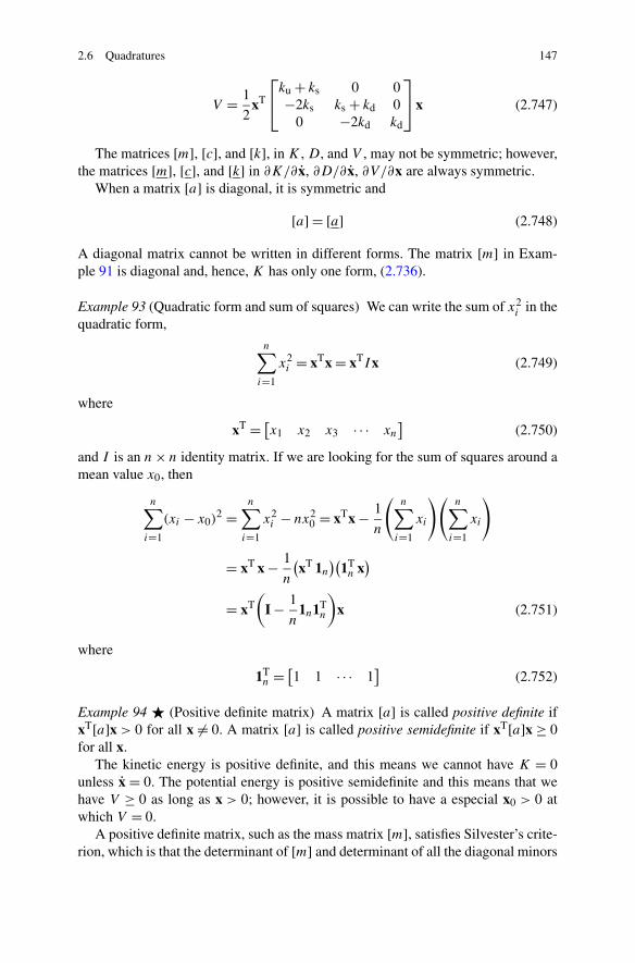
2.6 Quadratures 147
V = 1
2xT
⎡
⎣ku + ks 0 0−2ks ks + kd 0
0 −2kd kd
⎤
⎦x (2.747)
The matrices [m], [c], and [k], in K , D, and V , may not be symmetric; however,the matrices [m], [c], and [k] in ∂K/∂ x, ∂D/∂ x, ∂V/∂x are always symmetric.
When a matrix [a] is diagonal, it is symmetric and
[a] = [a] (2.748)
A diagonal matrix cannot be written in different forms. The matrix [m] in Exam-ple 91 is diagonal and, hence, K has only one form, (2.736).
Example 93 (Quadratic form and sum of squares) We can write the sum of x2i in the
quadratic form,
n∑
i=1
x2i = xTx = xTIx (2.749)
where
xT = [x1 x2 x3 · · · xn
](2.750)
and I is an n × n identity matrix. If we are looking for the sum of squares around amean value x0, then
n∑
i=1
(xi − x0)2 =
n∑
i=1
x2i − nx2
0 = xTx − 1
n
(n∑
i=1
xi
)(n∑
i=1
xi
)
= xT x − 1
n
(xT 1n
)(1Tn x
)
= xT(
I − 1
n1n1T
n
)x (2.751)
where
1Tn = [
1 1 · · · 1]
(2.752)
Example 94 � (Positive definite matrix) A matrix [a] is called positive definite ifxT[a]x > 0 for all x �= 0. A matrix [a] is called positive semidefinite if xT[a]x ≥ 0for all x.
The kinetic energy is positive definite, and this means we cannot have K = 0unless x = 0. The potential energy is positive semidefinite and this means that wehave V ≥ 0 as long as x > 0; however, it is possible to have a especial x0 > 0 atwhich V = 0.
A positive definite matrix, such as the mass matrix [m], satisfies Silvester’s crite-rion, which is that the determinant of [m] and determinant of all the diagonal minors
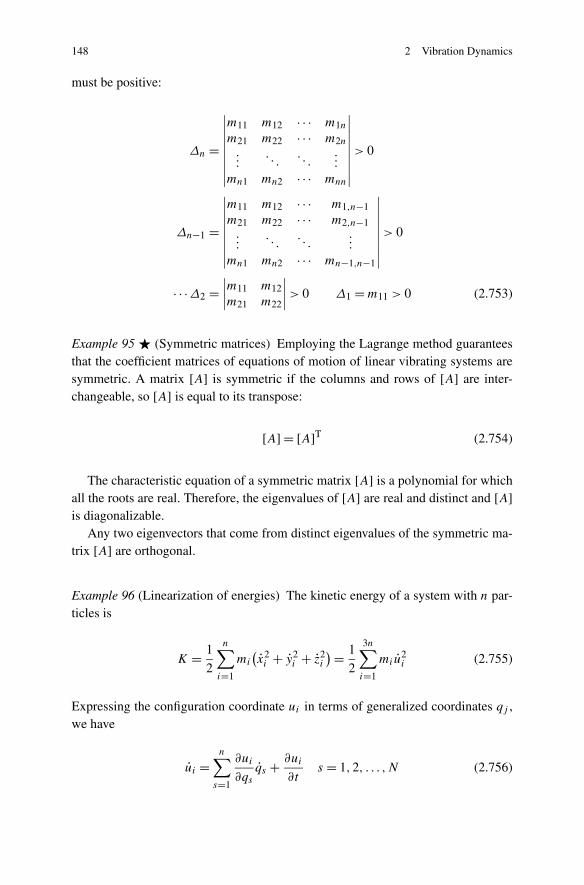
148 2 Vibration Dynamics
must be positive:
Δn =
∣∣∣∣∣∣∣∣∣
m11 m12 · · · m1n
m21 m22 · · · m2n
.... . .
. . ....
mn1 mn2 · · · mnn
∣∣∣∣∣∣∣∣∣
> 0
Δn−1 =
∣∣∣∣∣∣∣∣∣
m11 m12 · · · m1,n−1m21 m22 · · · m2,n−1...
. . .. . .
...
mn1 mn2 · · · mn−1,n−1
∣∣∣∣∣∣∣∣∣
> 0
· · ·Δ2 =∣∣∣∣m11 m12m21 m22
∣∣∣∣ > 0 Δ1 = m11 > 0 (2.753)
Example 95 � (Symmetric matrices) Employing the Lagrange method guaranteesthat the coefficient matrices of equations of motion of linear vibrating systems aresymmetric. A matrix [A] is symmetric if the columns and rows of [A] are inter-changeable, so [A] is equal to its transpose:
[A] = [A]T (2.754)
The characteristic equation of a symmetric matrix [A] is a polynomial for whichall the roots are real. Therefore, the eigenvalues of [A] are real and distinct and [A]is diagonalizable.
Any two eigenvectors that come from distinct eigenvalues of the symmetric ma-trix [A] are orthogonal.
Example 96 (Linearization of energies) The kinetic energy of a system with n par-ticles is
K = 1
2
n∑
i=1
mi
(x2i + y2
i + z2i
) = 1
2
3n∑
i=1
miu2i (2.755)
Expressing the configuration coordinate ui in terms of generalized coordinates qj ,we have
ui =n∑
s=1
∂ui
∂qs
qs + ∂ui
∂ts = 1,2, . . . ,N (2.756)
2.6 Quadratures 149
Therefore, the kinetic energy in terms of generalized coordinates is
K = 1
2
N∑
i=1
mi
(n∑
s=1
∂ui
∂qs
qs + ∂ui
∂t
)2
= 1
2
n∑
j=1
n∑
k=1
ajkqj qk +n∑
j=1
bj qj + c (2.757)
where
ajk =N∑
i=1
mi
∂ui
∂qj
∂ui
∂qk
(2.758)
bj =N∑
i=1
mi
∂ui
∂qj
∂ui
∂t(2.759)
c = 1
2
N∑
i=1
mi
(∂ui
∂t
)2
(2.760)
where
(n∑
s=1
∂ui
∂qs
qs + ∂ui
∂t
)2
=(
n∑
j=1
∂ui
∂qj
qj + ∂ui
∂t
)(n∑
k=1
∂ui
∂qk
qk + ∂ui
∂t
)
=n∑
j=1
n∑
k=1
(∂ui
∂qj
∂ui
∂qk
)qj qk
+ 2n∑
j=1
∂ui
∂qj
∂ui
∂tqj +
(∂ui
∂t
)2
(2.761)
Using these expressions, we may show the kinetic energy of the dynamic system:
K = K0 + K1 + K2 (2.762)
where
K0 = 1
2
N∑
i=1
mi
(∂ui
∂t
)2
(2.763)
K1 =n∑
j=1
N∑
i=1
mi
∂ui
∂qj
∂ui
∂tqj (2.764)
150 2 Vibration Dynamics
K2 = 1
2
n∑
j=1
n∑
k=1
N∑
i=1
mi
∂ui
∂qj
∂ui
∂qk
qj qk (2.765)
where
akj = ajk =N∑
i=1
mi
∂ui
∂qk
∂ui
∂qj
=N∑
i=1
mi
∂ui
∂qk
∂ui
∂qj
(2.766)
If the coordinates ui do not depend explicitly on time t , then ∂ui/∂t = 0, and wehave
K = K2 = 1
2
n∑
j=1
n∑
k=1
ajkqj qk = 1
2
n∑
j=1
n∑
k=1
∂2K(0)
∂qj ∂qi
qj qk
= 1
2
n∑
j=1
n∑
k=1
mij qj qk (2.767)
The kinetic energy is a scalar quantity and, because of (2.755), must be positivedefinite. The first term of (2.757) is a positive quadratic form. The third term of(2.757) is also a nonnegative quantity, as indicated by (2.760). The second term of(2.755) can be negative for some qj and t . However, because of (2.755), the sum ofall three terms of (2.757) must be positive:
K = 1
2qT[m]q (2.768)
The generalized coordinate qi represent deviations from equilibrium. The poten-tial energy V is a continuous function of generalized coordinates qi and, hence, itsexpansion is
V (q) = V (0) +n∑
i=1
∂V (0)
∂qi
qi + 1
2
n∑
j=1
n∑
i=1
∂2V (0)
∂qj ∂qi
qiqj + · · · (2.769)
where ∂V (0)/∂qi and ∂2V (0)/(∂qj ∂qi) are the values of ∂V/∂qi and ∂2V/(∂qj ∂qi)
at q = 0, respectively. By assuming V (0) = 0, and knowing that the first derivativeof V is zero at equilibrium
∂V
∂qi
= 0 i = 1,2,3, . . . , n (2.770)
we have the second-order approximation
V (q) = 1
2
n∑
j=1
n∑
i=1
kij qiqj (2.771)
2.7 Variational Dynamics 151
kij = ∂2V (0)
∂qj ∂qi
(2.772)
where kij are the elastic coefficients. The second-order approximation of V is zeroonly at q = 0. The expression (2.771) can also be written as a quadrature:
V = 1
2qT[k]q (2.773)
2.7 � Variational Dynamics
Consider a function f of x(t), x(t), and t :
f = f (x, x, t) (2.774)
The unknown variable x(t), which is a function of the independent variable t , iscalled a path. Let us assume that the path is connecting the fixed points x0 and xfduring a given time t = tf − t0. So x = x(t) satisfies the boundary conditions
x(t0) = x0 x(tf) = xf (2.775)
The time integral of the function f over x0 ≤ x ≤ xf is J (x) such that its valuedepends on the path x(t):
J (x) =∫ tf
t0
f (x, x, t)dt (2.776)
where J (x) is called an objective function or a functional.The particular path x(t) that minimizes J (x) must satisfy the following equation:
∂f
∂x− d
dt
∂f
∂x= 0 (2.777)
This equation is the Lagrange or Euler–Lagrange differential equation and is ingeneral of second order.
Proof To show that a path x = x�(t) is a minimizing path for the functional J (x) =∫ tft0
f (x, x, t)dt with boundary conditions (2.775), we need to show that
J (x) ≥ J(x�)
(2.778)
for all continuous paths x(t). Any path x(t) satisfying the boundary conditions(2.775) is called an admissible path. To see that x�(t) is the optimal path, we mayexamine the integral J for every admissible path. Let us define an admissible pathby superposing another admissible path y(t) onto x�,
x(t) = x� + εy(t) (2.779)

152 2 Vibration Dynamics
where
y(t0) = y(tf) = 0 (2.780)
and ε is a small parameter
ε � 1 (2.781)
Substituting x(t) in J of Eq. (2.776) and subtracting from J (x�) provides us withΔJ :
ΔJ = J(x� + εy(t)
)− J(x�)
=∫ tf
t0
f(x� + εy, x� + εy, t
)dt −
∫ tf
t0
f(x�, x�, t
)dt (2.782)
Let us expand f (x� + εy, x� + εy, t) about (x�, x�)
f(x� + εy, x� + εy, t
)
= f(x�, x�, t
)+ ε
(y
∂f
∂x+ y
∂f
∂x
)
+ ε2(
y2 ∂2f
∂x2+ 2yy
∂2f
∂x ∂x+ y2 ∂2f
∂x2
)dt + O
(ε3) (2.783)
and find
ΔJ = εV1 + ε2V2 + O(ε3) (2.784)
where
V1 =∫ tf
t0
(y
∂f
∂x+ y
∂f
∂x
)dt (2.785)
V2 =∫ tf
t0
(y2 ∂2f
∂x2+ 2yy
∂2f
∂x ∂x+ y2 ∂2f
∂x2
)(2.786)
The first integral, V1, is called the first variation of J , and the second integral, V2, iscalled the second variation of J . All the higher variations are combined and shownas O(ε3). If x� is the minimizing path, then it is necessary that ΔJ ≥ 0 for everyadmissible y(t). If we divide ΔJ by ε and make ε → 0, then we find a necessarycondition for x� to be the optimal path as V1 = 0. This condition is equivalent to
∫ tf
t0
(y
∂f
∂x+ y
∂f
∂x
)dt = 0 (2.787)
By integrating by parts, we may write
∫ tf
t0
y∂f
∂xdt =
(y
∂f
∂x
)tf
t0
−∫ tf
t0
yd
dt
(∂f
∂x
)dt (2.788)
2.7 Variational Dynamics 153
Because of y(t0) = y(tf) = 0, the first term on the right-hand side is zero. Therefore,the minimization integral condition (2.787) for every admissible y(t) reduces to
∫ tf
t0
y
(∂f
∂x− d
dt
∂f
∂x
)dt = 0 (2.789)
The terms in parentheses are continuous functions of t , evaluated on the optimal pathx�, and they do not involve y(t). Therefore, the only way for the bounded integralof the parentheses, (
∂f∂x
− ddt
∂f∂x
), multiplied by a nonzero function y(t) from t0 andtf, to be zero is
∂f
∂x− d
dt
∂f
∂x= 0 (2.790)
Equation (2.790) is a necessary condition for x = x�(t) to be a solution of the min-imization problem (2.776). This differential equation is called the Euler–Lagrangeor Lagrange equation. The second necessary condition to have x = x�(t) as a min-imizing solution is that the second variation, evaluated on x�(t), must be negative.
�
Example 97 � (Basic lemma) Consider two fixed points x1 and x2(> x1) and g(x)
as a continuous function for x1 ≤ x ≤ x2. If∫ x2
x1
f (x)g(x)dx = 0 (2.791)
for every choice of the continuous and differentiable function f (x) for which
f (x1) = f (x2) = 0 (2.792)
then
g(x) = 0 (2.793)
identically in x1 ≤ x ≤ x2. This result is called the basic lemma.To prove the lemma, let us assume that (2.793) does not hold. Therefore, suppose
there is a particular x0 of x in x1 ≤ x0 ≤ x2 for which g(x0) �= 0. At the moment,let us assume that g(x0) > 0. Because g(x) is continuous, there must be an intervalaround x0 such as x10 ≤ x0 ≤ x20 in which g(x) > 0 everywhere. However, (2.791)cannot then hold for every permissible choice of f (x). A similar contradiction isreached if we assume g(x0) < 0. Therefore, the lemma is correct.
Example 98 � (Lagrange equation for extremizing J = ∫ 21 x2 dt) The Lagrange
equation for extremizing the functional J ,
J =∫ 2
1x2 dt (2.794)
154 2 Vibration Dynamics
is∂f
∂x− d
dt
∂f
∂x= −x = 0 (2.795)
which shows that the optimal path is
x = C1t + C2 (2.796)
The boundary conditions x(1), x(2) provide C1 and C2. For example, assumingboundary conditions x(1) = 0, x(2) = 3 provides us with
x = 3t − 3 (2.797)
Example 99 � (Geodesics) The problem of determining the shortest path be-tween two given points at the same level of a quantitative characteristic is calledthe geodesic problem.
An example of a geodesic problem is: What is the shortest arc lying on the surfaceof a sphere and connecting two given points? We can generalize the problem asfollows.
Given two points on the surface of
g(x, y, z) = 0 (2.798)
what is the equation of the shortest arc lying on (2.798) and connecting the points?Let us express the equation of the surface in parametric form using parameters u
and v:
x = x(u, v) y = (u, v) z = z(u, v) (2.799)
the differential of the arc length may be written as
(ds)2 = (dx)2 + (dy)2 + (dz)2
= P(u, v)(du)2 + 2Q(u,v)dudv + R(u, v)(dv)2 (2.800)
where
P(u, v) =(
∂x
∂u
)2
+(
∂y
∂u
)2
+(
∂z
∂u
)2
(2.801)
R(u, v) =(
∂x
∂v
)2
+(
∂y
∂v
)2
+(
∂z
∂v
)2
(2.802)
Q(u,v) = ∂x
∂u
∂x
∂v+ ∂y
∂u
∂y
∂v+ ∂z
∂u
∂z
∂v(2.803)
If the curves u = const are orthogonal to the curves v = const, the quantity Q iszero. If the given fixed points on the surface are (u1, v1) and (u2, v2) with u2 > u1and we express the arcs and points by
v = v(u) v(u1) = v1 v(u2) = v2 (2.804)

2.7 Variational Dynamics 155
then the length of the arc is given by
J =∫ u2
u1
√
P(u, v) + 2Q(u,v)dv
du+ R(u, v)
(dv
du
)2
(2.805)
Our problem, then, is to find the function v(u) that renders the integral (2.805) aminimum. Employing the Lagrange equation, we find
∂P∂v
+ 2 dvdu
∂Q∂v
+ ( dvdu
)2 ∂R∂v
2√
P + 2Q dvdu
+ R( dv
du
)2− dv
du
(Q + R dv
du√P + 2Q dv
du+ R
( dvdu
)2
)= 0 (2.806)
In the special case where P , Q, and R are explicitly functions of u alone, this lastresult becomes
Q + R dvdu√
P + 2Q dvdu
+ R( dv
du
)2= C1 (2.807)
If the curves u = const are orthogonal to the curves v = const, we have
v = C1
∫ √P du√
R2 − C21R
(2.808)
Still supposing that Q = 0 but having P and R as explicit functions of v alone, wehave
u = C1
∫ √R dv√
P 2 − C21P
(2.809)
As a particular case let us consider the geodesic connecting two points on asphere with radius r . The most convenient parameters u and v for describing po-sition on the sphere surface are the colatitude θ and the longitude ϕ:
x = r cos θ sinϕ y = r sin θ sinϕ z = r cosϕ (2.810)
where θ is the angle between the positive z-axis and the line drawn from the spherecenter to the designated point and ϕ is the angle between the (x, z)-plane and thehalf plane bounded by the z-axis and containing the designated point. Therefore,
P = r2 sin2 θ R = r Q = 0 (2.811)
ϕ = C1
∫dv√
r2 sin4 θ − C21 sin2 θ
= − sin−1 cot θ√(r
C1
)2 − 1+ C2 (2.812)
from which it follows that
r sin θ cosϕ sinC2 − r sin θ sinϕ cosC2 − z√(r
C1
)2 − 1= 0 (2.813)

156 2 Vibration Dynamics
Fig. 2.39 A curve joiningpoints P1 and P2 and africtionless sliding point
Using (2.810) we find that the sphere geodesic lies on the following plane, whichpasses through the center of the sphere:
x sinC2 − y cosC2 − z√(r
C1
)2 − 1= 0 (2.814)
Therefore the shortest arc connecting two points on the surface of a sphere is theintersection of the sphere with the plane containing the given points and the centerof the sphere. Such an arc is called a great-circle arc.
Example 100 � (Brachistochrone problem) We may use the Lagrange equation andfind the frictionless curve joining points P1 and P2, as shown in Fig. 2.39, alongwhich a particle falling from rest due to gravity travels from the higher to the lowerpoint in minimum time. This is called the brachistochrone problem.
If v is the velocity of the falling point along the curve, then the time requiredto fall an arc length ds is ds/v. Then the objective function to find the curve ofminimum time is
J =∫ s2
s1
ds
v(2.815)
However,
ds =√
1 + y′2 dx y′ = dy
dx(2.816)
and according to the law of conservation of energy, we have
v = √2gy (2.817)
Therefore, the objective function simplifies to
J =∫ x2
x1
√1 + y′2
2gydx (2.818)
Applying the Lagrange equations, we find
y(1 + y′2) = 2R (2.819)

2.7 Variational Dynamics 157
where R is a constant. The optimal curve starting from y(0) = 0 can be expressedby the two parametric equations
x = R(θ − sin θ) y = R(1 − cos θ) (2.820)
The optimal curve is a cycloid.The name of the problem is derived from the Greek words “βραχιστoζ ,” mean-
ing “shortest,” and “χρoνoζ ,” meaning “time.” The brachistochrone problem wasoriginally discussed in 1630 by Galileo Galilei (1564–1642) and was solved in 1696by Johann and Jacob Bernoulli.
Example 101 � (Lagrange multiplier) Assume f (x) is defined on an open intervalx ∈ (a, b) and has continuous first and second-order derivatives in some neighbor-hood of x0 ∈ (a, b). The point x0 is a local extremum of f (x) if
df (x0)
dx= 0 (2.821)
Assume that f (x) = 0, x ∈Rn, and gi(x) = 0, i = 1,2, . . . , j , are functions defined
on an open region Rn and have continuous first- and second-order derivatives in R
n.The necessary condition that x0 is an extremum of f (x) subject to the constraintsgi(x) = 0 is that there exist j Lagrange multipliers λi , i = 1,2, . . . , j , such that
∇(s +
∑λigi
)= 0 (2.822)
For example, we can find the minimum of f ,
f = 1 − x21 − x2
2 (2.823)
subject to the constraint g
g = x21 + x2 − 1 = 0 (2.824)
by finding the gradient of f + λg:
∇(1 − x2
1 − x22 + λ
(x2
1 + x2 − 1)) = 0 (2.825)
which leads to
∂f
∂x1= −2x1 + 2λx1 = 0 (2.826)
∂f
∂x2= −2x2 + λ = 0 (2.827)
To find the three unknowns x1, x2, and λ, we employ Eqs. (2.826), (2.827), and(2.824). There are two sets of solutions as follows:
x1 = 0 x2 = 1 λ = 2x1 = ±1/
√2 x2 = 1/2 λ = 1
(2.828)

158 2 Vibration Dynamics
Fig. 2.40 Dido problem is tofind a planar curve y(x) witha constant length l tomaximize the enclosed area
Example 102 (Dido problem) Consider a planar curve y(x) with a constant length l
that connects the points (−R,0) and (R,0) as shown in Fig. 2.40. The Dido problemis to find the y(x) that maximized the enclosed area. The objective function of theDido problem is
J =∫ R
−R
y dx (2.829)
However, the constant length provides us with a constraint equation:
l =∫ R
−R
ds =∫ R
−R
√1 + y′2 dx (2.830)
ds =√
1 + y′2 dx y′ = dy
dx(2.831)
Therefore, using the Lagrange multiplier λ, the objective function with constraintwould be
J =∫ R
−R
(f(y, y′, x
)+ λg(y, y′, x
))dx (2.832)
f = y g =√
1 + y′2 (2.833)
The Lagrange equation for the constraint objective function (2.832) is
∂f
∂y− d
dx
∂f
∂y′ + λ
(∂g
∂y− d
dx
∂g
∂y′
)= 0 (2.834)
Equation (2.834) leads to
1
λ= d
dx
y′√
1 + y′2 (2.835)
This differential equation must be solved to determine the maximizing curve y(x).First integration provides us with
λy′√
1 + y′2 = x + C1 (2.836)
2.7 Variational Dynamics 159
Solving this equation for y′ yields
y′ = ±(x + C1)√λ2 − (x + C1)
(2.837)
and a second integration yields
y = ±√
λ2 − (x + C1) + C2 (2.838)
Satisfying the boundary conditions (−R,0) and (R,0), we have
C1 = C2 = 0 λ = R (2.839)
which indicates that the function y(x) is
x2 + y2 = R2 (2.840)
It is a circle with center at O and radius R.
Example 103 � (Several independent variables) We now derive the differen-tial equations that must be satisfied by the twice-differentiable functions q1(t),q2(t), . . . , qn(t) that extremize the integral J :
J =∫ t2
t1
f (q1, q2, . . . , qn, q1, q2, . . . , qn, t)dt (2.841)
The functions q1(t), q2(t), . . . , qn(t) achieve given the values at the fixed limits ofintegration t1 and t2, where t1 < t2.
Let us show the optimal functions by q�i (t), i = 1,2, . . . , n. We may examine
the integral J for every admissible function. An admissible function may be definedby
qi(t) = q�i + εyi(t) (2.842)
where
yi(t1) = yi(t2) = 0 (2.843)
and ε is a small parameter,
ε � 1 (2.844)
Consider a function f = f (qi, qi , t). The variables qi(t) satisfy the boundary con-ditions
q1(t1) = q1 q(t2) = q2 (2.845)
160 2 Vibration Dynamics
Substituting qi(t) in J and subtracting from (2.841) yields
ΔJ = J(q�i + εyi(t)
)− J(q�i
)
=∫ tf
t0
f(q�i + εyi, q
�i + εyi , t
)dt −
∫ tf
t0
f(q�i , q
�i , t
)dt (2.846)
Let us expand f (x� + εy, x� + εy, t) about (x�, x�):
f(q�i + εyi, q
�i + εyi , t
)
= f(q�i , q
�i , t
)+ ε
(yi
∂f
∂qi
+ yi
∂f
∂qi
)
+ ε2(
y2i
∂2f
∂q2i
+ 2yi yj
∂2f
∂qi ∂qj
+ y2i
∂2f
∂q2i
)dt
+ O(ε3) (2.847)
and find
ΔJ = εV1 + ε2V2 + O(ε3) (2.848)
where
V1 =∫ tf
t0
(yi
∂f
∂qi
+ yj
∂f
∂qj
)dt (2.849)
V2 =∫ tf
t0
(y2i
∂2f
∂q2i
+ 2yi yj
∂2f
∂qi ∂qj
+ y2i
∂2f
∂q2i
)(2.850)
If we divide ΔJ by ε and make ε → 0, then we find a necessary condition V1 = 0for q
�i to be the optimal path. By integrating V1 by parts, we may write
∫ tf
t0
y1∂f
∂q1dt =
(y1
∂f
∂q1
)t2
t1
−∫ t2
t1
y1d
dt
(∂f
∂q1
)dt (2.851)
Since y1(t1) = y2(t2) = 0, the first term on the right-hand side is zero and the inte-gral of V1 reduces to
∫ t2
t1
y1
(∂f
∂q1− d
dt
∂f
∂q1
)dt = 0 (2.852)
The terms in parentheses are continuous functions of t evaluated on the optimal pathx�, and they do not involve y1(t). So, the only way for the bounded integral of theparentheses, (
∂f∂q1
− ddt
∂f∂q1
), multiplied by a nonzero function y1(t) to be zero is ifthe parentheses are zero. Therefore, the minimization integral condition for everyadmissible y1(t) is
∂f
∂q1− d
dt
∂f
∂q1= 0 (2.853)
2.8 Key Symbols 161
Using a similar treatment of the successive pairs of terms of (2.851), we derive thefollowing n conditions to minimize (2.841):
∂f
∂qi
− d
dt
∂f
∂qi
= 0 i = 1,2, . . . , n (2.854)
Therefore, when a definite integral is given which contains n functions to be deter-mined by the condition that the integral be stationary, we can vary these functionsindependently. So, the Euler–Lagrange equation can be formed for each functionseparately. This provides us with n differential equations.
2.8 Key Symbols
a ≡ x accelerationa, b distance, Fourier series coefficientsa, b,w,h lengtha accelerationA,B weight factor, coefficients for frequency responsesc damping[c] damping matrixce equivalent dampingC mass centerd position vector of the body coordinate framedf infinitesimal forcedm infinitesimal massdm infinitesimal momentE mechanical energy, Young modulus of elasticityf = 1/T cyclic frequency [Hz]f,F, f,F forceFC Coriolis forceg gravitational accelerationH heightI moment of inertia matrixI1, I2, I3 principal moment of inertiak stiffnesske equivalent stiffnesskij element of row i and column j of a stiffness matrix[k] stiffness matrixK kinetic energyl directional lineL moment of momentumL= K − V Lagrangeanm massme eccentric mass, equivalent mass
162 2 Vibration Dynamics
mij element of row i and column j of a mass matrixmk spring massms sprung mass[m] mass matrixn number of coils, number of decibels, number of noteN natural numbersp pitch of a coilP powerr frequency ratior position vectort timet0 initial timeT periodTn natural periodv ≡ x,v velocityV potential energyx, y, z,x displacementx0 initial displacementx0 initial velocityx, y, z velocity, time derivative of x, y, z
x accelerationX amplitude of x
z relative displacement
Greek
α,β, γ angle, angle of spring with respect to displacementδ deflection, angleδs static deflectionε mass ratioθ angular motion coordinateω,ω,Ω angular frequencyϕ,Φ phase angleλ eigenvalue
2.9 Exercises
1. Equation of motion of vibrating systems.Determine the equation of motion of the systems in Figs. 2.41(a) and (b) by
(a) using the energy method(b) using the Newton method(c) using the Lagrange method
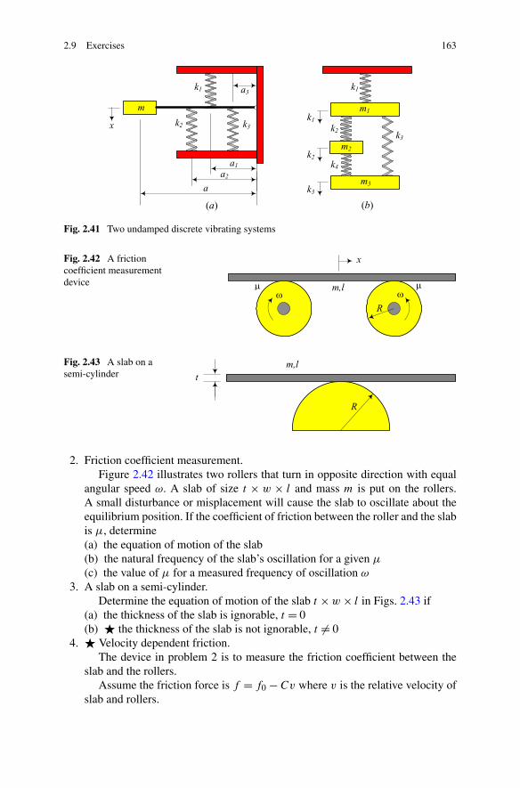
2.9 Exercises 163
Fig. 2.41 Two undamped discrete vibrating systems
Fig. 2.42 A frictioncoefficient measurementdevice
Fig. 2.43 A slab on asemi-cylinder
2. Friction coefficient measurement.Figure 2.42 illustrates two rollers that turn in opposite direction with equal
angular speed ω. A slab of size t × w × l and mass m is put on the rollers.A small disturbance or misplacement will cause the slab to oscillate about theequilibrium position. If the coefficient of friction between the roller and the slabis μ, determine(a) the equation of motion of the slab(b) the natural frequency of the slab’s oscillation for a given μ
(c) the value of μ for a measured frequency of oscillation ω
3. A slab on a semi-cylinder.Determine the equation of motion of the slab t × w × l in Figs. 2.43 if
(a) the thickness of the slab is ignorable, t = 0(b) � the thickness of the slab is not ignorable, t �= 0
4. � Velocity dependent friction.The device in problem 2 is to measure the friction coefficient between the
slab and the rollers.Assume the friction force is f = f0 − Cv where v is the relative velocity of
slab and rollers.

164 2 Vibration Dynamics
Fig. 2.44 Spring connectedpendulum
(a) Determine the equation of motion of the slab if x and x are assumed small.(b) Determine the equation of motion of the slab if x is comparable with Rω.(c) Determine the equation of motion of the slab if one roller is turning with
angular speed of 2ω, assuming x is very small.5. Moving on x-axis.
The displacement of a particle moving along the x-axis is given by
x = 0.01t4 − t3 + 4.5t2 − 10 t ≥ 0
(a) Determine t1 at which x becomes positive.(b) For how long does x remain positive after t = t1?(c) How long does it take for x to become positive for the second time?(d) When and where does the particle reach its maximum acceleration?(e) Derive an equation to calculate its acceleration when its speed is given.
6. � Kinetic energy of a rigid link.Consider a straight and uniform bar as a rigid link of a manipulator. The link
has a mass m. Show that the kinetic energy of the bar can be expressed as
K = 1
6m(v1 · v1 + v1 · v2 + v2 · v2)
where v1 and v2 are the velocity vectors of the end points of the link.7. Ideal spring connected pendulum.
Determine the kinetic and potential energies of the pendulum in Fig. 2.44, atan arbitrary angle θ . The free length of the spring is l = a − b.
8. � General spring connected pendulum.Determine the potential energy of the pendulum in Fig. 2.44, at an angle θ ,
if:(a) The free length of the spring is l = a − 1.2b.(b) The free length of the spring is l = a − 0.8b.
9. � Moving on a cycloid.A particle is moving on a planar curve with the following parametric expres-
sion:
x = r(ωt − sinωt) y = r(1 − cosωt)
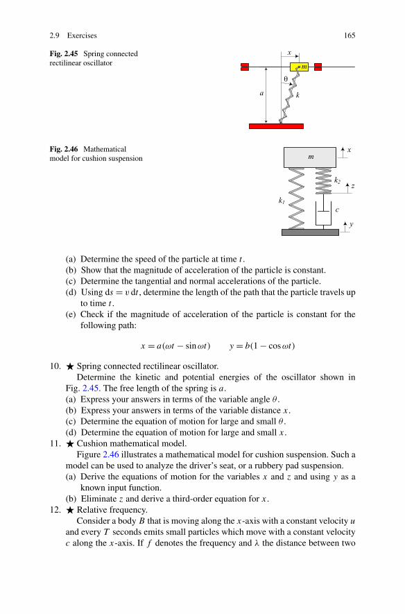
2.9 Exercises 165
Fig. 2.45 Spring connectedrectilinear oscillator
Fig. 2.46 Mathematicalmodel for cushion suspension
(a) Determine the speed of the particle at time t .(b) Show that the magnitude of acceleration of the particle is constant.(c) Determine the tangential and normal accelerations of the particle.(d) Using ds = v dt , determine the length of the path that the particle travels up
to time t .(e) Check if the magnitude of acceleration of the particle is constant for the
following path:
x = a(ωt − sinωt) y = b(1 − cosωt)
10. � Spring connected rectilinear oscillator.Determine the kinetic and potential energies of the oscillator shown in
Fig. 2.45. The free length of the spring is a.(a) Express your answers in terms of the variable angle θ .(b) Express your answers in terms of the variable distance x.(c) Determine the equation of motion for large and small θ .(d) Determine the equation of motion for large and small x.
11. � Cushion mathematical model.Figure 2.46 illustrates a mathematical model for cushion suspension. Such a
model can be used to analyze the driver’s seat, or a rubbery pad suspension.(a) Derive the equations of motion for the variables x and z and using y as a
known input function.(b) Eliminate z and derive a third-order equation for x.
12. � Relative frequency.Consider a body B that is moving along the x-axis with a constant velocity u
and every T seconds emits small particles which move with a constant velocityc along the x-axis. If f denotes the frequency and λ the distance between two
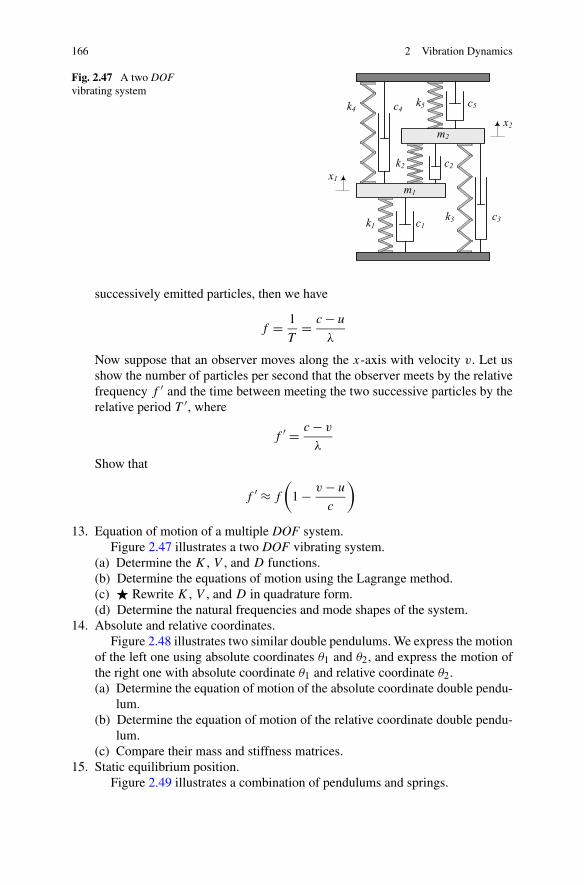
166 2 Vibration Dynamics
Fig. 2.47 A two DOFvibrating system
successively emitted particles, then we have
f = 1
T= c − u
λ
Now suppose that an observer moves along the x-axis with velocity v. Let usshow the number of particles per second that the observer meets by the relativefrequency f ′ and the time between meeting the two successive particles by therelative period T ′, where
f ′ = c − v
λ
Show that
f ′ ≈ f
(1 − v − u
c
)
13. Equation of motion of a multiple DOF system.Figure 2.47 illustrates a two DOF vibrating system.
(a) Determine the K , V , and D functions.(b) Determine the equations of motion using the Lagrange method.(c) � Rewrite K , V , and D in quadrature form.(d) Determine the natural frequencies and mode shapes of the system.
14. Absolute and relative coordinates.Figure 2.48 illustrates two similar double pendulums. We express the motion
of the left one using absolute coordinates θ1 and θ2, and express the motion ofthe right one with absolute coordinate θ1 and relative coordinate θ2.(a) Determine the equation of motion of the absolute coordinate double pendu-
lum.(b) Determine the equation of motion of the relative coordinate double pendu-
lum.(c) Compare their mass and stiffness matrices.
15. Static equilibrium position.Figure 2.49 illustrates a combination of pendulums and springs.

2.9 Exercises 167
Fig. 2.48 Two similar doublependulums, expressed byabsolute and relativecoordinates
Fig. 2.49 A combination ofpendulums and springs
Fig. 2.50 An elasticpendulum
(a) Determine the value of equilibrium θ0 and static stretch of spring δ0 if weassemble the system and let it go slowly.
(b) Determine the equation of motion of the system in terms of x measuredfrom the shown equilibrium position.
(c) Determine the equation of motion of the system in terms of y.16. Elastic pendulum.
Figure 2.50 illustrates an elastic pendulum. Such a pendulum has two DOF.(a) Determine the equations of motion using the energy method.(b) Determine the equations of motion using the Lagrange method.(c) Determine the equations of motion using the Newton–Euler method.(d) Linearize the equations of motion.
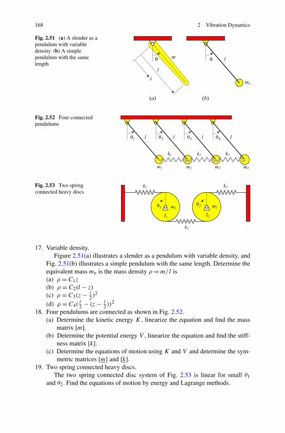
168 2 Vibration Dynamics
Fig. 2.51 (a) A slender as apendulum with variabledensity. (b) A simplependulum with the samelength
Fig. 2.52 Four connectedpendulums
Fig. 2.53 Two springconnected heavy discs
17. Variable density.Figure 2.51(a) illustrates a slender as a pendulum with variable density, and
Fig. 2.51(b) illustrates a simple pendulum with the same length. Determine theequivalent mass me is the mass density ρ = m/l is(a) ρ = C1z
(b) ρ = C2(l − z)
(c) ρ = C3(z − l2 )2
(d) ρ = C4(l2 − (z − l
2 ))2
18. Four pendulums are connected as shown in Fig. 2.52.(a) Determine the kinetic energy K , linearize the equation and find the mass
matrix [m].(b) Determine the potential energy V , linearize the equation and find the stiff-
ness matrix [k].(c) Determine the equations of motion using K and V and determine the sym-
metric matrices [m] and [k].19. Two spring connected heavy discs.
The two spring connected disc system of Fig. 2.53 is linear for small θ1
and θ2. Find the equations of motion by energy and Lagrange methods.
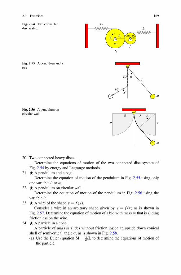
2.9 Exercises 169
Fig. 2.54 Two connecteddisc system
Fig. 2.55 A pendulum and apeg
Fig. 2.56 A pendulum oncircular wall
20. Two connected heavy discs.Determine the equations of motion of the two connected disc system of
Fig. 2.54 by energy and Lagrange methods.21. � A pendulum and a peg.
Determine the equation of motion of the pendulum in Fig. 2.55 using onlyone variable θ or ϕ.
22. � A pendulum on circular wall.Determine the equation of motion of the pendulum in Fig. 2.56 using the
variable θ .23. � A wire of the shape y = f (x).
Consider a wire in an arbitrary shape given by y = f (x) as is shown inFig. 2.57. Determine the equation of motion of a bid with mass m that is slidingfrictionless on the wire.
24. � A particle in a cone.A particle of mass m slides without friction inside an upside down conical
shell of semivertical angle α, as is shown in Fig. 2.58.(a) Use the Euler equation M = d
dtL to determine the equations of motion of
the particle.

170 2 Vibration Dynamics
Fig. 2.57 A wire of theshape of y = f (x)
Fig. 2.58 A particle of massm slides inside a conical shell
Fig. 2.59 A particle on a circular surface
(b) Show that it is possible for the particle to move such that it is at a constantR with the cone axis.
(c) Determine the angular speed of the particle for a uniform motion of part (b).25. � A particle on a circular surface.
Draw FBD of the particle in Figs. 2.59(a) and (b) for a = cR, c < 1, anddetermine their equation of motion. The spring is linear and applies a tangentialforce on m.
26. � Falling on a spring.A solid mass m falls on a spring as shown in Fig. 2.60(a) or with a spring
as shown Fig. 2.60(b). The spring exerts a stiffness force Fs. Determine themaximum compression xMax of the springs if:(a) The restitution coefficient e = 0 and Fs = kx.(b) The restitution coefficient e = 0 and Fs = kx3.(c) The restitution coefficient e = 1 and Fs = kx3.
We define a restitution coefficient e by v′2 − v′
1 = e(v1 − v2),0 ≤ e ≤ 1,where v1, v2 are the speed of the two particles before impact and v′
1, v′2 are their
speeds after impact. The case e = 1 indicates an inelastic collision in which theparticles stick to each other after impact, and the case e = 0 is called the plasticcollision in which the energy conserves in impact.
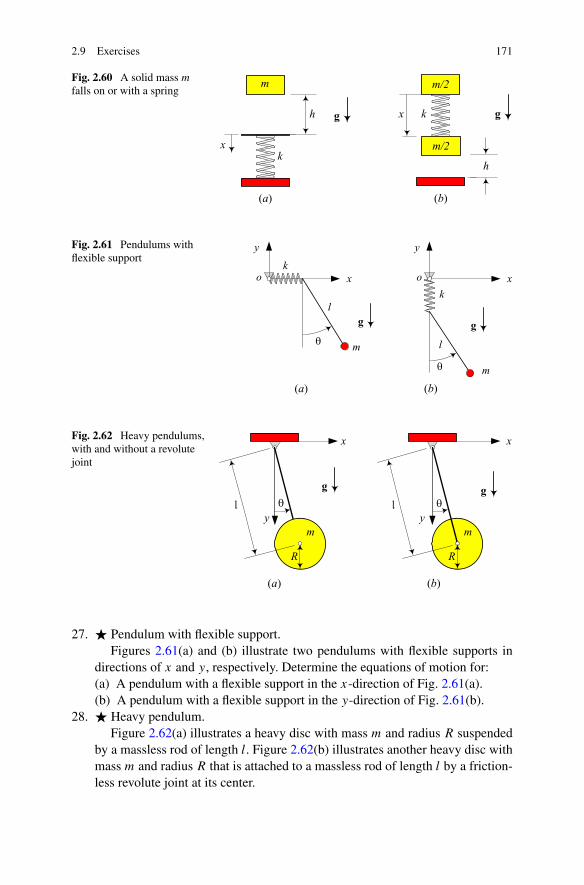
2.9 Exercises 171
Fig. 2.60 A solid mass m
falls on or with a spring
Fig. 2.61 Pendulums withflexible support
Fig. 2.62 Heavy pendulums,with and without a revolutejoint
27. � Pendulum with flexible support.Figures 2.61(a) and (b) illustrate two pendulums with flexible supports in
directions of x and y, respectively. Determine the equations of motion for:(a) A pendulum with a flexible support in the x-direction of Fig. 2.61(a).(b) A pendulum with a flexible support in the y-direction of Fig. 2.61(b).
28. � Heavy pendulum.Figure 2.62(a) illustrates a heavy disc with mass m and radius R suspended
by a massless rod of length l. Figure 2.62(b) illustrates another heavy disc withmass m and radius R that is attached to a massless rod of length l by a friction-less revolute joint at its center.
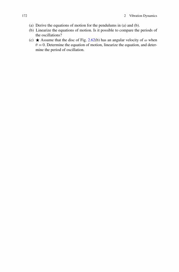
172 2 Vibration Dynamics
(a) Derive the equations of motion for the pendulums in (a) and (b).(b) Linearize the equations of motion. Is it possible to compare the periods of
the oscillations?(c) � Assume that the disc of Fig. 2.62(b) has an angular velocity of ω when
θ = 0. Determine the equation of motion, linearize the equation, and deter-mine the period of oscillation.
http://www.springer.com/978-1-4614-4159-5