VibeBin: A Vibration-Based Waste Bin Level Detection System

122

VibeBin: A Vibration-Based Waste Bin Level Detection System

YIRAN ZHAO, University of Illinois at Urbana-Champaign

SHUOCHAO YAO, University of Illinois at Urbana-Champaign

SHEN LI, IBM Research

SHAOHAN HU, IBM Research

HUAJIE SHAO, University of Illinois at Urbana-Champaign

TAREK F. ABDELZAHER, University of Illinois at Urbana-Champaign

This paper presents the design and implementation of VibeBin, a low-cost, non-intrusive and easy-to-install waste binlevel detection system. Recent popularity of Internet-of-Things (IoT) sensors has brought us unprecedented opportunitiesto enable a variety of new services for monitoring and controlling smart buildings. Indoor waste management is crucialto a healthy environment in smart buildings. Measuring the waste bin fill-level helps building operators schedule garbagecollection more responsively and optimize the quantity and location of waste bins. Existing systems focus on directly andintrusively measuring the physical quantities of the garbage (weight, height, volume, etc.) or its appearance (image), andtherefore require careful installation, laborious calibration or labeling, and can be costly. Our system indirectly measures

fill-level by sensing the changes in motor-induced vibration characteristics on the outside surface of waste bins. VibeBinexploits the physical nature of vibration resonance of the waste bin and the garbage within, and learns the vibration featuresof different fill-levels through a few garbage collection (emptying) cycles in a completely unsupervised manner. VibeBinidentifies vibration features of different fill-levels by clustering historical vibration samples based on a custom distance metric

which measures the dissimilarity between two samples. We deploy our system on eight waste bins of different types and sizes,and show that under normal usage and real waste, it can deliver accurate level measurements after just 3 garbage collectioncycles. The average F-score (harmonic mean of precision and recall) of measuring empty, half, and full levels achieves 0.912. Atwo-week deployment also shows that the false positive and false negative events are satisfactorily rare.

CCS Concepts: •Computing methodologies →Unsupervised learning; Cluster analysis;

General Terms: Design, Algorithms

Additional Key Words and Phrases: Internet-of-Things, Smart Building, Waste Management, Wireless sensors

ACM Reference format:

Yiran Zhao, Shuochao Yao, Shen Li, Shaohan Hu, Huajie Shao, and Tarek F. Abdelzaher. 2017. VibeBin: A Vibration-BasedWaste Bin Level Detection System. PACM Interact. Mob. Wearable Ubiquitous Technol. 1, 3, Article 122 (September 2017),22 pages.DOI: 10.1145/3132027

1 INTRODUCTION

The proliferation of Internet-of-Things (IoT) sensors has made our indoor environment smarter. Various sensing

and communication techniques spawn new services for monitoring the buildings we stay in. Among these

This work was supported in part by NSF grants CNS 16-18627, CNS 13-20209, CNS 13-29886 and CNS 13-45266.

ACM acknowledges that this contribution was authored or co-authored by an employee, or contractor of the national government. As such,

the Government retains a nonexclusive, royalty-free right to publish or reproduce this article, or to allow others to do so, for Government

purposes only. Permission to make digital or hard copies for personal or classroom use is granted. Copies must bear this notice and the

full citation on the first page. Copyrights for components of this work owned by others than ACMmust be honored. To copy otherwise,

distribute, republish, or post, requires prior specific permission and/or a fee. Request permissions from [email protected].

© 2017 ACM. 2474-9567/2017/9-ART122 $15.00

DOI: 10.1145/3132027

on Interactive, Mobile, Wearable and Ubiquitous Technologies, Vol. 1, No. 3, Article 122. Publication date: September 2017.

122:2 • Y. Zhao et al.

services, waste management is important, since an average US adult spends 87% of their time indoors [13].

Garbage that accumulates around indoor areas is unsanitary and unhealthy. If not cleaned in a timely manner,

the overflow of garbage can be a serious problem. However, cleaning incurs expensive human labor. VibeBin

is designed to reduce unnecessary labor by moving from a fixed garbage collection schedule towards a more

on-demand paradigm, where labor is incurred only when needed. It also helps reduce the use of plastic bags,

optimize the quantity of waste bins and reallocate the bins according to their utilization.

Few existing solutions for waste bin level monitoring systems have managed to simultaneously achieve low cost,

ease of installation, absence of labeling or calibration, and high accuracy. Many systems rely on cameras [3, 8, 9]

or some combination of ultrasonic sensors, proximity sensors, weight sensors, and even pressure and temperature

sensors [2, 24]. Although they claim to achieve high accuracy, these systems need careful installation, manual

calibration, and/or labeling of training data. In addition, some systems are intrusive, meaning that the devices are

installed inside the bin or under the lid, which can be smudged or damaged from direct contact with garbage.

Our system is low-cost because we only use an off-the-shelf accelerometer and a $1.95 vibration motor. It can

also be easily installed by anybody without complicated instructions. To allow such convenience with just one

sensor, we design VibeBin to be able to learn from vibration samples of each individual bin and make accurate

measurements for that same bin as soon as possible. The contributions of our work are thus threefold:

(1) To the best of our knowledge, this is the first work that exploits the physical nature of vibration resonance

to measure the waste bin fill-level. We describe the physical model of our system and show how we

utilize the vibration features in real examples.

(2) We build a low-cost, non-intrusivewaste bin fill-level detection system that can be easily and incrementally

deployed on existing waste bins. Our system does not require expensive hardware and can be general

enough to work on a wide variety of waste bins.

(3) Our system is completely free of the need for labeling or calibration. We show how it automatically

learns the vibration features as the fill-level changes, and show that it can make accurate measurements

after just 3 waste collection cycles (usually within a week) with real garbage.

The rest of the paper is organized as follows. Section 2 describes a system overview and provides a physical model of our system. In Section 3, we show the design of system hardware and software and elaborate on the learning process. Section 4 evaluates our system in real deployment. In Section 5, we summarize the lessons learned. Section 6 discusses related work and Section 7 concludes this paper.

2 OVERVIEW

VibeBin enables the scenario where janitors are able to see the most recent fill-level of every waste bin on their smartphones. The backend server collects vibration samples from each bin and runs our algorithm to tell whether the bin is empty, half full, or full. The smartphone communicates with the server to retrieve the waste bin status and display it on the building map. In this way, only those full waste bins need attention.

VibeBin learns the fill-levels by learning the characteristics of vibration caused by a vibrating mini motor. As shown in Figure 1, the accelerometer is firmly glued to the outside surface of the waste bin, and the vibration motor is firmly attached to a lower position. The motor’s vibration direction should be perpendicular to the bin surface so that the vibration force can be effectively applied to the surface. The motor is connected to the device’s digital-to-analog output pin, so as VibeBin applies an increasing voltage to the motor, the frequency and intensity of the motor vibration also increase. Due to complex interactions of the garbage and waste bin, the vibration intensity sensed by the accelerometer does not always keep increasing, but sometimes decreases as the voltage increases. We model this phenomenon as forced vibration with damping, where a local vibration maximum is a point of resonance.

VibeBin monitors the fill-level by waking up regularly and taking a sample of vibration local maxima, which consists of several pairs of voltage and vibration intensity. It then sends the sample to the backend server to


A Vibration-Based Waste Bin Level Detection System • 122:3

Garbage

VibrationDC Motor

Accelerometer andWireless device

Backend server

- +

Waste bin

WiFi

Fig. 1. System overview. Fig. 2. System workflow.

be stored. As the fill-level changes, the resonant voltage and intensity also change because the damping effect

of the garbage is different. Figure 2 shows the workflow of our system. The backend server collects samples

generated in a few garbage collection cycles, and learns the fill-level in a completely unsupervised manner. This is

achieved by a customized clustering method that divides samples into several groups, each representing a certain

garbage fill-level. The clustering results are then analyzed to find recurring empty-to-full cycles automatically,

and level numbers are assigned to each group. Next, representative samples are selected from each group to form

profiles of different levels. Finally new samples collected can be matched to the historical profiles to determine

the current waste bin fill-level.

2.1 The underlying physics

When the device is taking a sample, it linearly increases the motor voltage from the threshold (1.2V) to the

maximum (3.7V). We normalize this voltage range into the range from 0.0 to 1.0 spaced by 0.02. Let V denote the

normalized voltage (or voltage in short). The intensity I at each voltage V is the mean acceleration magnitude,

which is calculated by adjusting the accelerometer readings to have zero mean and taking the average of the

absolute values of acceleration. The motor rotation speed ω is roughly linear to input voltage [30], so we regard

ω to be proportional to V .

Under the rotation speed of ω, the vibration force F of the motor is F = C1 × ω2 [33], where C1 is a constant

coefficient. We omit the detailed expressions for constant values C1, and C2, C3, C4, C5 (which are used below),

because it does not affect our understanding of the underlying physics. Interested readers can refer to physics

theories [29, 31, 32]. According to the theory of resonance [31], when an object oscillates in a damping situation

under external sinusoidal force F , the mean amplitude of the oscillation is A(ω) = C2F ÷ (√

(1 − r 2)2 + (2ζ r )2),where r = ω

ωn, ωn is the natural frequency of the waste bin surface under interactions with garbage, ζ is the

damping ratio. Further, ωn =√

km, k is the spring constant in kд/s2,m is the equivalent mass of the vibrating

part of bin surface and garbage as a whole. And ζ = c

2√km

where c is the damping coefficient, which increases

as the garbage fills up. Then, the mean oscillation velocity is proportional to A(ω)ω and the mean oscillation

acceleration is proportional to A(ω)ω2 [29]. Therefore the intensity I can be expressed in the following equation.

I (ω) = C3A(ω)ω2 = C4ω4

√(1 − r 2)2 + (2ζ r )2

= C4ω4

√(1 − ω2m

k)2 + c2ω2

k2

(1)



The spring constant k represents the material’s stiffness, which equals to the force divided by the displacement

caused by the force. Suppose a 100N force deforms the material by 0.01m, then k = 104 N /m. ζ is smaller than 1

because the bin surface oscillation is always under-damped [32]. When ωn and ζ are fixed, r = ωωn

and ζ is small,

the local maximum is obtained when rmax ≈ 1 + 3ζ 2, and Imax ≈ C5ω4n

ζ= 2C5

k2.5

m1.5c. Taking a reasonable example,

letm ∈ [0.5,2] (kд), c ∈ [3,11] (kд/s), then the relationship of I and ω is shown in Figure 3. When the fill-level

increases, the general trend is thatm increases and the damping coefficient c also increases, so Imax is expected

to decrease. The motor spins at 137Hz (3.7 volt) and the natural oscillation frequency of garbage and waste bin is

generally less than 100Hz, so in most cases there exists a local maximum. If not, the global maximum is taken as

its vibration intensity.

0 50 100 150 200 250 3000

2

4

6

8

10

(1/s)

I

(m,c) pairs (0.5,3)

(0.5,5)

(0.5,7)(0.5,9)(0.5,11)

(1.0,3)

(1.5,3)

(2.0,3)

I

2

Fig. 3. Example of the relationship of I and ω.

0 0.1 0.2 0.3 0.4 0.5 0.6 0.7 0.8 0.9 10

1

2

3

4

5

V

I (

cm/s

)2

V1 V2

I1

I2

Fig. 4. A real example of I and V .

In reality, as V increases, there might be multiple local maxima. Figure 4 shows a real example, where there

are two local maxima (V1, I1) = (0.36,1.17) and (V2, I2) = (0.78,4.40). A possible explanation is that the bin has

multiple surfaces, each surface is under different interactions with the garbage, therefore the vibration of all

surfaces as a whole can have multiple resonant points. But since each local maxima represents a feature, the

device sends all local maxima (V , I ) pairs to the backend server. The unsupervised learning is possible because

the waste bin is emptied regularly, and the vibration features recur every cycle. Although the empty state of the

waste bin is not always exactly the same, we discover that the resonance voltage is very similar every time and

the intensity is always the largest.

2.2 Design considerations

There are several considerations when designing and building this system.

(1) Easy to install. This is the most important consideration since we are not building specialized waste

bins, but are installing sensing devices on many existing waste bins. Intrusive sensors such as ultrasonic

sensors and proximity sensors need to be carefully installed inside the waste bin. They need precise

hardware installation and software calibration. VibeBin is designed to be easy to install and non-intrusive.

It can be superglued to the outside surface of the waste bin with the motor being certain distance below

the accelerometer. The distance is not important to the unsupervised learning process, but we usually

use 20cm to 50cm.

(2) Learning fast. Since VibeBin learns the fill-levels without any human labeling effort, the learning speed

is a concern. VibeBin has to learn by itself from a few garbage collection cycles and be able to make

measurements as soon as possible.

(3) Low power consumption. VibeBin device belongs to a type of Internet-of-Things (IoT) sensor, and must

be energy efficient and long lasting. VibeBin device requires a battery to operate, but changing battery

should not be as frequent as every few weeks. VibeBin saves energy by putting itself in deep sleep mode

most of the time and only waking up for a few seconds each time to take a sample.



(4) Low cost. For large deployment and possibility of vandalism or theft, the cost should be as low as possible.

VibeBin is assembled using off-the-shelf components, including a $17.1 Particle Photon device, a $21.21

inertial measurement unit (IMU), a $10.49 10,000mAh 3.7V lithium battery (from a power bank) and a

$1.95 vibrating mini motor. The total commercial selling price is only around $50.75, which is much

cheaper compared to the total cost of $560 in Table III of [2].

(5) Minimal data transmission. Although the IoT device we use does not have wireless bandwidth constraint,

we still pursue minimal data transmission because other weaker IoT devices that can be used to replace

Photon might have limited transmission capability. The only data for transmission in each wake up is

several (V , I ) pairs, along with meta data such as device ID and waste bin ID. The transmitted data in a

character stream is only around 50 bytes.

3 SYSTEM DESIGN

3.1 System hardware and software

Figure 5 shows hardware installation on four waste bins, the installation of other waste bins is similar and there

is no strict installation rule. The main computing device Particle Photon has a Broadcom WICED Wi-Fi chip

alongside a powerful STM32 ARM Cortex M3 microcontroller (MCU) running at 120MHz. It has 1MB flash and

128KB memory. When the Photon device is operating with WiFi connected, it draws 80mA current. When it

is put into deep sleep mode, it only consumes about 0.08mA. The Photon device is stacked onto a SparkFun

LSM9DS1 IMU shield, which has a 3-axis accelerometer sampling at 952Hz. We only use the z-axis since it is

perpendicular to the waste bin surface. The IMU shield draws 0.6mA current and keeps sampling for only a few

seconds each time.

The mini vibration motor is connected to the 8-bit digital-to-analog output pin of the Photon device, where the

maximum voltage is 3.7 volt. At 3.7V, the motor draws around 60mA current. At each voltage V , Photon reads 50

IMU readings in about 0.05s, and calculates the intensity I of the correspondingV . The time of sweeping through

the 50 voltages is about 2.5 seconds. Then the system scans the intensity values of the 50 voltages and finds all

local maxima, which constitute a sample Xi . In most cases, each sample only consists of 1 to 3 local maxima.

The time duration of deep sleep is determined empirically. It is not necessary to wake up too often since the

fill-level may not change. But if it sleeps too long, certain states of the waste bin may be missed. Photon has

the ability to adjust the sleep time itself and retain some variables saved last time before sleep. So we set the

sleeping time to be either 15 minutes or 30 minutes, depending on the dissimilarity of the current sample and the

last saved sample. The dissimilarity is measured by distance in Section 3.2.1, and empirically, if the distance is

greater than 0.1, it sleeps for 15 minutes, otherwise it sleeps for half an hour. So each day there are around 50-100

Fig. 5. Hardware prototype installation on the waste bins. We name them Bin1, Bin2, Bin3 and Bin7 from left to right.



samples sent to the backend server. To determine the lifespan of a fully charged battery, we experimented on a

smaller 300mAh battery. It lasted 10 days and sent 738 samples. So with a 10,000mAh battery it can last around

10 months.

The software, excluding the operating system, consumes only 18KB of RAM and 97KB of ROM. The C++ code

and the firmware can be flashed via Particle cloud platform [21]. The program uses one array to store the IMU

readings, which are only 50 float numbers. The vibration intensity values calculated from the IMU readings are

then stored in another array of 50 float numbers, each represents the intensity of the corresponding voltage.

Then the program makes a one-pass scan of this array to find all local maxima points. A valid local maximum

should be greater than its previous and next 5 points, to reduce fake ones. Then the system sends the sample to

the backend server using TCP socket connection. Since there is no hard time deadline for measurements, the

backend server can be a regular desk top or even an IoT embedded system [35] which has shown capabilities of

running even complex deep learning models [34]. The server stores historical samples of all waste bins registered

under this server. The backend server applies our algorithm to historical samples of each individual bin and

automatically learns the features of different fill-levels, and will be able to make measurements after only a few

garbage collection cycles.

3.2 Learning from historical samples

The collected samples on the server are ordered by timestamp. Denote the i-th sample as Xi = {(V ni , I

ni ),n =

1,2...,N }, where N is the number of local maxima in Xi . Suppose the (V , I ) pairs are sorted by V (V ni < Vm

i for

any n < m). The first step is to filter the samples which contains large intensity values because someone happens

to be moving the waste bin when the device is taking a sample. A sample is deleted if its maximum intensity value

is larger than twice the maximum intensity values in both its previous and following samples. These abnormal

samples are less than one percent because the “sense and then sample” scheme is used to make sure the bin stays

still before sampling, so the probability of someone moving the bin during the 2.5-second sampling period is low.

We first plot an example of historical samples from 5 empty-to-full cycles in Figure 6. The x-axis is the sample

number (i), blue dots are voltages (V ni ) and green crosses are vibration intensity values (Ini ). I is shown in cm/s2

to avoid large decimal places. The samples start with empty state and experienced 5 garbage collection cycles,

where the emptying action point is indicated by the purple vertical lines.

0 50 100 150 200 250 300 350−1

−0.5

0

0.5

1

Vo

lta

ge

V

Samples0 50 100 150 200 250 300 350

0

14.21

28.42

Inte

nsity

I (

cm/s

)

Empty Empty Empty ...Full Full

2

Fig. 6. Bin1: historical samples. In this example, the empty level has 2 resonance points, one peaks at V1 ≈ 0.2 and I1 ≈ 11, another at V2 ≈ 0.75 and I2 ≈ 26. Full level typically has 1 global maximum point, V3 ≈ 1 and I3 ≈ 14. From empty to full, both voltage (blue dots) and intensity (green crosses) at vibration maximum change. The largest peak intensity (I2) decreases as garbage level fills up, and the smaller resonance peak (V1) disappears.

Proceedings of the ACM on Interactive, Mobile, Wearable and Ubiquitous Technologies, Vol. 1, No. 3, Article 122. Publication date: September 2017.


We observe that the features of every empty level are quite similar. There are two local maxima, and the second

resonance voltage (V ≈ 0.75) has the largest vibration intensity value since there is no garbage that dampens the

vibration. As the waste bin fills up, the features of fuller levels can exhibit slightly different progress, but the

general trend is that the peak vibration intensity is decreasing (reflected by green crosses going down). Therefore,

if we knew the features of empty and full levels, given a new sample, the system should be able to match it

to some previous samples of a certain level, and tell the user the current fill-level. Therefore, clustering and

classification of samples is a fundamental task.

The core of our algorithm is to automatically classify samples into empty, full and some intermediate levels.

We define a customized distance metric between two samples, and employ a distance matrix based K-means

for clustering. For example, given two empty-level samples X1 = {(V 11 = 0.21, I 11 = 12), (V 2

1 = 0.75, I 21 = 25)}and X2 = {(V 1

2 = 0.22, I 12 = 11), (V 22 = 0.78, I 22 = 26)}, the distance should be small since the two (V , I ) pairs are

both similar. For two full-level samples such as X3 = {(V 13 = 1.0, I 13 = 12)} and X4 = {(V 1

4 = 0.98, I 14 = 14)}, theirdistance should also be small. For an empty-level sample X1 and a full-level sample X3, both V and I values arevery different, so the distance should be large. We define the distance in Section 3.2.1.

3.2.1 Definition of the distance between two samples. Suppose the two samples are X1 = {(Vm1 , I

m1 ),m =

1,2...,N1} and X2 = {(V n2 , I

n2 ),n = 1,2...N2}. Since N1 and N2 can be greater than 1 and can be different, there

are many ways to match the N1 pairs in X1 with N2 pairs in X2. When matching the (V , I ) pairs between two

samples, the relative order of (V , I ) pairs within each sample needs to stay the same. It means when matching

(Vm1

1 , Im1

1 ) with (V n12 , I

n12 ) and (Vm2

1 , Im2

1 ) with (V n22 , I

n22 ), ifm1 < m2 then n1 < n2. Also, the matching process is

supposed to be strict rather than to minimize the average matching distance, meaning that the first match with

the smallest distance should be fixed, and then recursively continue matching the rest of the pairs (instead of

enumerating all possible ways of matching and finding the minimum overall distance). So first we calculate the

N1 × N2 matching matrix A of {(Vm1 , I

m1 ),m = 1,2...,N1} and {(V n

2 , In2 ),n = 1,2...,N2} where Amn is the distance

between (Vm1 , I

m1 ) and (V n

2 , In2 ), and is defined as:

d ((Vm1 , I

m1 ), (V n

2 , In2 )) =

|Vm1 −V n

2 |max (Vm

1 ,Vn2 )+

|Im1 − In2 |max (Im1 , I

n2 )

(2)

Taking maximum at the denominator is to normalize the difference, sinceV and I are on different scales. Because

N1 can be different from N2, there may be some (V , I ) pairs left unmatched. Unmatched (V , I ) should also

contribute to the distance, which is:

d ′((V , I )) =I

Imax+

V

1.0(3)

Where Imax is the maximum intensity seen in any of the two samples. The reason to choose Imax and 1.0

as denominators is that if the unmatched V and I are small, then the unmatched pair does not make the two

samples significantly different because larger pairs are matched perfectly. If the unmatched pair has large V and

I , then the two samples should has larger distance. Algorithm 1 explains the process of matching and distance

calculation given the matching matrix A. First, the algorithm finds the minimum element in A to be Amn , and

fixes the matching between (Vm1 , I

m1 ) with (V n

2 , In2 ). It cumulates the distance between (Vm

1 , Im1 ) and (V n

2 , In2 ), and

recursively perform the matching of the rest of the pairs, which are {(V i1 , I

i1 ),i = 1,2...,m − 1} matching with

{(V j2 , I

j2 ), j = 1,2...,n − 1}, and {(V i

1 , Ii1 ),i =m + 1, ...,N1} matching with {(V j

2 , Ij2 ), j = n + 1, ...,N2}. Counting the

number of distance values cumulated from both matched pairs and unmatched pairs, it equals to max(N1,N2).

The final distance score is the average of these distance values. Note that in Algorithm 1, we use MatLab syntax

to denote a submatrix (A1 and A2).

For example, X1 = {(0.21,12),(0.75,25)}, X2 = { (0.22,11), (0.78,26)} and X3 = {(1.0,12)}. To calculate the

distance between X1 and X2, we can easily see that our algorithm would match (0.21,12) with (0.22,11), and match



ALGORITHM 1: Calculating the distance between a pair of samples.

Input: Matrix A (N1 by N2), X1 and X2.

Output: distance(X1,X2).

distance(X1,X2)=Distance(A)+UnmatchedDistance(X1,X2 )

max (N1,N2 );

DISTANCE(A):if A has 0 row or 0 column then

return 0;

end

Amn=findMinimumElement(A);

distance = Amn=d ((Vm1 , Im1 ), (V n2 , I

n2 )); (Equ. (2))

A1=A(1 : m − 1,1 : n − 1);

A2=A(m + 1 : N1,n + 1 : N2);

return distance+Distance(A1)+Distance(A2);

UNMATCHEDDISTANCE(X1,X2):

Imax =max (Iji ); (i = 1,2; 1 ≤ j ≤ Ni )

distance = 0;

for unmatched (V , I ) in X1 and X2 dodistance +=d ′((V , I )); (Equ. (3))

end

return distance;

(0.75,25) with (0.78,26). So the distance is ( 12−1112 +0.22−0.21

0.22 + 26−2526 +

0.78−0.750.78 ) ÷max (2,2) = 0.1. To calculate the

distance between X1 and X3, our algorithm would match (0.75,25) with (1.0,12) and (0.21,12) is unmatched. So the

distance is ( 25−1225 +1−0.75

1 + 1225 +

0.211 ) ÷max (2,1) = 0.73.

Our definition of distance satisfies d (x ,x ) = 0, non-negativity (d (x1,x2) ≥ 0) and symmetry (d (x1,x2) = d (x2,x1)), but does not strictly satisfy the triangle inequality (d (x1,x2) + d (x2,x3) ≥ d (x1,x3)). However, when N1 = N2 = N3 = 1 and V1 = V2 = V3 = V , it does satisfy the triangle inequality. To prove this, suppose X1 = {(V , I1)}, X2 = {(V , I2)} and X3 = {(V , I3)}, and suppose I1 < I2 < I3. Then to satisfy the triangle inequality we need I2

I−2

I1 + I3I−3

I2 > I3I−3

I1 , which can be easily proven. In practice, we find that our definition of distance works well in clustering.

3.2.2 Clustering samples. After calculating the distance between every pair of historical samples, we cluster the samples into several groups, each representing a certain fill-level. Clustering turns raw samples into a sequence of cluster numbers, which makes it easier to identify cycles and classify clusters into correct fill-levels.The approach is a customized distance matrix based K-means. We choose the number of clusters to be 6 for the following reasons.

Choosing K = 2 is too coarse. Perhaps for the user, giving two levels (empty and full) might be enough. But it will be hard to find the emptying action because the class number might jump frequently between empty and full (jitters) when the fill-level is somewhere in the middle. K = 3 can be enough for some cases, because a jump from level 3 to level 1 can be identified as the emptying action. However, some waste bins have more diverse resonance features, and clustering into only 3 groups makes it difficult to select representative samples (Section 3.2.4). Because each cluster may actually contain some smaller clusters within, and ignoring them makes the selection process biased. Therefore, we can consider larger K . From user’s perspective, we want to give empty, half and full 3 levels, so we let K be a multiple of three (six is our choice). Further increasing K may result in too many empty clusters, especially when each garbage collection cycle only consists of less than 100 samples.



As we know, K-means clustering result depends on the initialization of each sample’s membership. Random

initialization can work but may not necessarily yield good results. Besides, random initialization also means that

each time the program runs, it is likely to generate different clusters. This instability makes the results hard to

reproduce, and also makes it look inconsistent when showing the intermediate results in our system demo [36].

Therefore, we use UPGMA (Unweighted Pair Group Method with Arithmetic Mean) algorithm [26] to generate

initial membership matrix. UPGMA is a simple agglomerative hierarchical clustering algorithm that merges

samples into six clusters given their distance matrix. The quality of these six clusters is not as good as K-means,

but it serves as a good initialization. In this way the initial membership matrix stays the same, and the clustering

results of K-means will be stable and better. Our customized K-means is different from traditional K-means in

that there is no representation of cluster center (mean). Our K-means is similar to kernel K-means algorithm

[28], but differs in that our distance matrix does not satisfy the properties of a kernel matrix. Nevertheless our

algorithm works well in practice.

Suppose the historical sample set is X = {xi ,i = 1,2, ...,N } (we use small x to denote each sample this time).

We derive the N by N distance matrix S, where Si j=distance(xi ,x j ) according to Algorithm 1. The input to the

K-means algorithm is S and initial membership matrix. The number of clusters K = 6.

The K-means algorithm divides X into K disjoint clusters {Ck ,k = 1,2, ...,K }, each cluster Ck has a virtual

centermk . We can calculate the similarity of sample xi to the centermk in a way akin to kernel K-means algorithm

[28], which is:

simi (xi ,mk ) = Sii − 2

∑Nj=1 O (x j ∈ Ck )Si j∑Nj=1 O (x j ∈ Ck )

+

∑Nj=1

∑Nl=1 O (x j ∈ Ck )O (xl ∈ Ck )Sjl∑N

j=1

∑Nl=1 O (x j ∈ Ck )O (xl ∈ Ck )

(4)

Where O (Y ) = 1 if Y is true and 0 otherwise. According to this equation, sample xi is assigned to Ck where

simi (xi ,mk ) is the largest. Now we explain the algorithm in matrix form. Suppose U is the K by N membership

matrix, where∑Kk=1 Uki = 1 and Uki = 1 if xi belongs to Ck . Our K-means algorithm is described in Algorithm 2.

ALGORITHM 2: Customized K-means algorithm.

Input: S, X , initial U.

Output: U.

converдe = false;

while converдe == false do

for xi ∈ X do

Calculate simi (xi ,mk ) for all k ;

Update Uki = 1 if simi (xi ,mk ) is the largest;

end

if U does not change then

converдe=true;

end

end

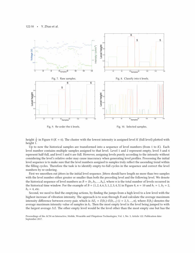
We show the clustering results of Bin2 in Figure 8, the raw samples of which are shown in Figure 7. Each color

(height) in Figure 8 represents a cluster, which is explained in the following section.

3.2.3 Processing clustering results. After initial clustering, we calculate the average maximum intensity of

samples in each cluster, and assign initial level numbers to clusters according to their intensity level. For example,

the cluster in which samples have the highest intensity is assigned to be level 1 (empty level), and is plotted with


122:10 • Y. Zhao et al.

0 20 40 60 80 100 120 140−1

−0.5

0

0.5

1

Vol

tage

(V

)

Samples0 20 40 60 80 100 120 1400

13.7

27.5

41.4

Inte

nsity

I (c

m/s

)2

Fig. 7. Raw samples.

0 20 40 60 80 100 120 140

0

0.2

0.4

0.6

0.8

1

Leve

l hei

ght

Samples

6

5 5

Fig. 8. Classify into 6 levels.

0 20 40 60 80 100 120 140

0

0.2

0.4

0.6

0.8

1

Leve

l hei

ght

Samples

5

6 6

Fig. 9. Re-order the 6 levels.

0 20 40 60 80 100 120 140

0

0.2

0.4

0.6

0.8

1

Samples

Leve

l hei

ght

Fig. 10. Selected samples.

1Kheight in Figure 8 (K = 6). The cluster with the lowest intensity is assigned level K (full level) plotted with

height 1.Up to now the historical samples are transformed into a sequence of level numbers (from 1 to K). Each

level number contains multiple samples assigned to that level. Level 1 and 2 represent empty, level 3 and 4 represent half-full, and level 5 and 6 are full. However, assigning levels purely according to the intensity without considering the level’s relative order may cause inaccuracy when generating level profiles. Processing the initial level sequence is to make sure that the level numbers assigned to samples truly reflect the ascending trend within the filling cycles. Therefore the task is to identify empty-to-full cycles in the sequence and correct the level numbers by re-ordering.

First we smoothen out jitters in the initial level sequence. Jitters should have length no more than two samples with the level number either greater or smaller than both the preceding level and the following level. We denote the historical sequence of level numbers as B = {b1,b2, ...,bn }, where n is the total number of levels occurred in the historical time window. For the example of B = {1,2,4,6,5,1,2,3,4,5} in Figure 8, n = 10 and b1 = 1, b2 = 2, b3 = 4, etc.

Second, we need to find the emptying actions, by finding the jumps from a high level to a low level with the highest increase of vibration intensity. The approach is to scan through B and calculate the average maximum intensity difference between every pair, which is ΔEi = E (bi )−E (bi−1) (i = 2,3, ...,n), where E (bi ) denotes the average maximum intensity value of samples in bi . Then the most empty level is the level being jumped to with the largest average ΔE. The other empty level would be the level other than the most empty one but has the



largest maximum intensity. For example, in Figure 8, the jump from level 5 to level 1 at sample number 82 is the

largest, so level 1 is the most empty. Then level 2 would be the second empty level. Let eset be the empty level set.

In our example, eset = {1,2}.Third, we cut the historical level sequence B into shorter rising segments {Bi ,i = 1,2, ...}, so that each segment

Bi starts with a level from eset , and ends right before the level returns to lower than K2 after experiencing levels

higher than 2K3 . For the example in Figure 8, B1 = {1,2,4,6,5} and B2 = {1,2,3,4,5}. The reason to analyze those

rising segments is to see if we need to re-assign (re-order) a few level numbers to make the level sequences in

better ascending order. This re-ordering helps improve level profile accuracy. For example, comparing Figure 8

and Figure 9, level 5 and 6 are reordered (exchanged level numbers) to better reflect the empty-to-full trend.

The re-ordering process first derives the global order of initial level numbers, and then re-assigns a few level

numbers to better reflect the overall ascending trend in each cycle. To derive a global order from the partial

order in {Bi , i = 1,2...} is challenging. The first challenge is that the number of segments is small, since the

learning process has to complete within just a few empty-to-full cycles. The second challenge is that in each Bi ,some levels might be absent. Therefore, calculating pairwise transition probability and finding the most likely

permutation may be problematic due to insufficient transition cases to derive meaningful statistics. Instead, we

use some heuristics to reorder level numbers. First, the transition matrix T is obtained from all segments where

Tmn is the number of times levelm is followed by level n. But finding the global level order solely from T is not

stable since not all level transitions are present. So we use T to insert absent levels in each Bi if the absent levelscan be transitioned from or to a level in Bi . If not, the absent level is inserted in a way that tries to preserve the

initially assigned order. After inserting all absent levels, the segment Bi becomes a completed segment.

To explain in more detail, given Bi , we first calculate each level’s average position. For example, if Bi ={1,2,1,2,3}, level 1 has average position 1+3

2 = 2, level 2 has average position 2+42 = 3, and level 3 has 5. Then a

deduplicated version of partial order Hi is derived from Bi based on the level’s average position (Hi = {1,2,3}).The next task is to find absent levels inHi and insert them according to T. If level k is absent inHi = {b1,b2, ...,bn },we check Tbjk and Tkbj (1 ≤ j ≤ n) to see if level k can be after bj or before bj , and choose a more likely position

to insert. If Tbjk > Tkbj then insert k after bj ; if Tbjk < Tkbj then insert k before bj . If Tbjk = Tkbj , k is inserted

before bj if k < bj , or after bj if k > bj . If there is no bj in Hi such that Tbjk > 0 or Tkbj > 0, a default position is

to insert k between bj and bj+1 where bj < k < bj+1.For the example in Figure 8, H1 = {1,2,4,6,5} and H2 = {1,2,3,4,5}. Level 3 is absent in H1, and 6 is absent

in H2. The transition matrix T23 = 1, and T34 = 1, T65 = 1, T46 = 1, then we insert level 3 after level 2 and thus

H1 = {1,2,3,4,6,5}, and insert level 6 after level 4 and thus H2 = {1,2,3,4,6,5}. After applying this step to all

{Hi ,i = 1,2, ...}, we have a collection of completed segments. Therefore we can calculate the average position

of each levels from the completed segments, and output the global order of the initial level numbers. Then the

level numbers are reordered to make the global order strictly increasing. For example, {1,2,3,4,6,5} will become

{1,2,3,4,5,6} by exchanging level number 5 and 6. After re-ordering, the classification is complete and each

cluster is assigned with the best possible level number.

3.2.4 Sample selection and profile generation. After classification, VibeBin generates profiles for each level

by selecting representative samples. And new samples are compared to each level profile to decide the current

waste bin level. It is not optimal to compare each new sample to all historical samples in each level. Because

jitters that are smoothened out and samples that are far from its cluster center should not be in the profile. So we

select a few representative samples in each level. We empirically set the number of representative samples to be

10 for each level. For each level we select a random sample within the historical time window and store it in an

array of its level. The array is sorted so that samples having larger similarity (Equation (4)) to their cluster center

are preferred. The random selection is continued until each level has twice the desired number of samples, and

the best 10 samples are chosen to represent that level. If the number of available samples in a certain level is not


122:12 • Y. Zhao et al.

0 50 100 150 200 250 300−1

−0.5

0

0.5

1

Vol

tage

(V

)

Samples0 50 100 150 200 250 300

0

5.2714

10.5428

15.8143

Inte

nsity

I (c

m/s

)2Window 1

Window 2

Cycle 1 Cycle 2 Cycle 3 Cycle 4 Cycle 5

Fig. 11. Raw samples.

0 20 40 60 80 100 120 140 160

0

0.2

0.4

0.6

0.8

1

Samples

Leve

l hei

ght

6

Fig. 12. Results of time window 1.

40 60 80 100 120 140 160 180 200 220

0

0.2

0.4

0.6

0.8

1

Leve

l hei

ght

Samples

4

6

Fig. 13. Results of time window 2.

enough, all samples are selected. It is allowed that a certain level contains zero sample, meaning that the profile of a certain level can be empty. A profile is named using a version number and a level number, and contains the selected samples in it. The version is assigned according to the current time window, which is explained in the next section.

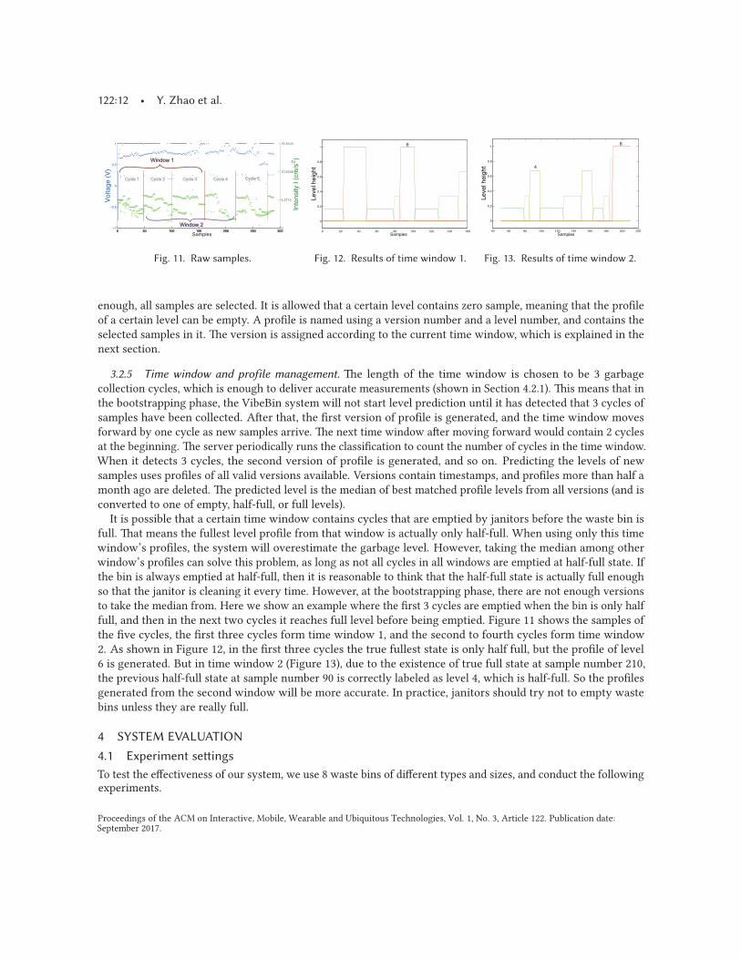
3.2.5 Time window and profile management. The length of the time window is chosen to be 3 garbage collection cycles, which is enough to deliver accurate measurements (shown in Section 4.2.1). This means that in the bootstrapping phase, the VibeBin system will not start level prediction until it has detected that 3 cycles of samples have been collected. After that, the first version of profile is generated, and the time window moves forward by one cycle as new samples arrive. The next time window after moving forward would contain 2 cycles at the beginning. The server periodically runs the classification to count the number of cycles in the time window. When it detects 3 cycles, the second version of profile is generated, and so on. Predicting the levels of new samples uses profiles of all valid versions available. Versions contain timestamps, and profiles more than half a month ago are deleted. The predicted level is the median of best matched profile levels from all versions (and is converted to one of empty, half-full, or full levels).It is possible that a certain time window contains cycles that are emptied by janitors before the waste bin is

full. That means the fullest level profile from that window is actually only half-full. When using only this time window’s profiles, the system will overestimate the garbage level. However, taking the median among other window’s profiles can solve this problem, as long as not all cycles in all windows are emptied at half-full state. If the bin is always emptied at half-full, then it is reasonable to think that the half-full state is actually full enough so that the janitor is cleaning it every time. However, at the bootstrapping phase, there are not enough versions to take the median from. Here we show an example where the first 3 cycles are emptied when the bin is only half full, and then in the next two cycles it reaches full level before being emptied. Figure 11 shows the samples of the five cycles, the first three cycles form time window 1, and the second to fourth cycles form time window 2. As shown in Figure 12, in the first three cycles the true fullest state is only half full, but the profile of level 6 is generated. But in time window 2 (Figure 13), due to the existence of true full state at sample number 210, the previous half-full state at sample number 90 is correctly labeled as level 4, which is half-full. So the profiles generated from the second window will be more accurate. In practice, janitors should try not to empty waste bins unless they are really full.

4 SYSTEM EVALUATION4.1 Experiment settingsTo test the effectiveness of our system, we use 8 waste bins of different types and sizes, and conduct the following experiments.



Fig. 14. Metal boiler.

0 20 40 60 80 100 120−1

−0.5

0

0.5

1

Vol

tage

V

Samples0 20 40 60 80 100 120

0

0.725

1.45

Inte

nsity

I (

cm/s

）2

Fig. 15. Metal boiler raw samples.

0 20 40 60 80 100 120

0

0.2

0.4

0.6

0.8

1

Sample number

Lev

el h

eigh

t

Fig. 16. Metal boiler: classification.

Fig. 17. A glass jug.

0 20 40 60 80 100 120 140−1

−0.5

0

0.5

1

Vol

tage

V

Samples0 20 40 60 80 100 120 140

0

0.9

1.8

Inte

nsity

I (

cm/s

)2

Fig. 18. Glass jug raw samples.

0 20 40 60 80 100 120 140

0

0.2

0.4

0.6

0.8

1glass

Sample number

Lev

el h

eigh

t

Fig. 19. Glass jug: classification.

(1) We let the bins experience normal 4 empty-to-full cycles with real garbage, and then manually test the

level measurement accuracy using similar garbage. The garbage people throw into the bins is common

daily trash (such as trash found in shopping areas), including but not limited to food waste, fruit, vegetable

peels, paper, boxes, bottles and cans.

(2) We use the previously generated level profiles to test the measurement accuracy for light weight garbage,

such as empty bottles, cartons and cans. We show that light weight garbage still cause vibration changes

despite their low density.

(3) We deploy the bins for another 2 weeks, and collect garbage by ourselves when a certain bin indicates

full. False positive is the case when the bin is indicating full but is actually empty. To find out the false

negatives, we examine each bin twice each day, to check whether a bin is full but is not indicating full.

First check is early afternoon and second check is early evening.

The details of the 8 bins are as follows. Bin1, Bin5, Bin6, Bin7 and Bin8 are smaller ones and Bin2, Bin3 and

Bin4 are relatively bigger. The size is given as height × circumference (at top). Bin1 measures 33cm × 70cm, Bin2

is 84cm × 90cm, Bin3 is 73cm × 97cm, Bin4 is 80cm × 87cm, Bin5 is 34cm × 70cm, Bin6 is 40cm × 77cm, Bin7 is

34cm × 75cm, and Bin8 is 44cm × 85cm. Bin1, Bin5, Bin7 and Bin8 are made of soft and thin plastic material and

Bin6 is made of stiff and thicker plastic material. Bin2, Bin3 and Bin4 are made of hard plastic materials, and Bin3

has a lid.

Indoor waste bins are generally made of plastic materials, but we want to test the feasibility of our system on

bins made of other materials. We did not find waste bins made of glass or steel, so we tested our system on other

similar containers shown in Figure 14 and Figure 17. We install the sensors in the same way and gradually fill

them with water for 2 cycles. The samples are plotted in Figure 15 and Figure 18 while the level classification

results are in Figure 16 and Figure 19. We can see that our methodology is general enough to work with a wide

variety of materials.

For the first experiment, we let the waste bins normally experience four empty-to-full cycles with real trash.

The only ground truth we collect is the time of garbage collections (emptying actions), which are shown as dark

vertical lines in the samples figures. However, none of the ground truth is used in the learning process in any


16

122:14 • Y. Zhao et al.

way. Shown in Section 4.2.1, 3 cycles are enough to deliver good measurements, which takes about a week. For testing, we take around 30-40 samples each time when the waste bin is filled with little garbage (as empty), around half filled, and when it is full. We repeat taking samples 3 times in the 3 different cycles, each time the fill-level is not exactly the same. We run the algorithm to assign the level numbers to the test samples using the level profiles generated from the four cycles, and calculate the measurement accuracy. The reason that we do not make measurements in finer granularity is the following. First, the learning process is unsupervised, and there is no labeled sample for training as in other common machine learning scenarios. Even if the classification divides the state into 6 levels, the difference of the amount of garbage between adjacent levels is not necessarily . So it is reasonable to just measure empty, half, and full three levels. Second, from the users’ perspective, it is not necessary to distinguish, for example, 40% full from 60% full, because there is no action needed anyway. What we care is, how many times when the actual state is full but it measures half-full, or how many times when the state is half-full but it measures full. Therefore, the main result we examine is the accuracy of measurements and the confusion matrix of the 3 levels shown in Section 4.2.2.For the second experiment, we found enough empty plastic water bottles, milk cartons and soda cans to test

the measurement accuracy of light weight garbage. Similar to the first experiment, we take around 30-40 samples for each level in each cycle and repeat 3 cycles. We use the level profiles generated in the first experiment under normal denser garbage to test the samples collected under light weight garbage. We show the confusion matrix of the 3 levels in Section 4.2.3.

For the third experiment, we put the bins under normal usage for the duration of two weeks and monitor the status of each bin as samples are collected. If a particular bin shows three consecutive full-level samples, we go to the site and empty the bin. Each time of garbage collection, we record the true perceived fill-level of the bin in order to find out false positives. In the early afternoon and early evening of each day, we check if there are false negatives. The results are shown in Section 4.2.4, and the reason for choosing two weeks as the experiment period is also explained there.

4.2 Evaluation results4.2.1 How soon to make accurate measurements. After the system is installed, there is a bootstrapping phase

to learn the waste bin levels before being able to make accurate measurements. If the system cannot make good measurements after a long time, users may lose interest in our system. We run the algorithm after experiencing 1, 2, 3 and 4 cycles and use the learning results to classify test samples and calculate the measurement accuracy for each of the three levels. Shown in Figure 20, averaging the accuracy of eight waste bins, we can see that after 3 cycles, the system is already able to make accurate measurements, with detecting full level at more than 90%accuracy (or recall percentage). Therefore, as described in Section 3.2.5, the historical time window is set to be 3 cycles.

4.2.2 Measurement accuracy for real garbage. We show the measurement precision and recall on the test samples. The confusion matrix for each waste bin is listed in Table 1, where the i-th row and j-th column is the number of times level i is measured as level j.

We first look at the most important number in the confusion matrix, that is the third row and second column, which means how many times the waste bin is full but is measured as only half-full. Two small bins (Bin5 and Bin8) have more cases of misclassifying full level as half-full (recall rate is about 85%). On the one hand, for small bins it is harder to control the difference between half-full and full when testing. On the other hand, the amount of garbage in small bins is not significant, and the height of small bins is short, so the vibration feature difference is not significant. But the recall rate of full state for large waste bins are satisfying. Bin2, Bin3 and Bin4 have only around 4% misclassification on full state on average. This is because big bins have significantly more garbage to



Table 1. Confusion matrices of measuring the levels of normal garbage.

(a) Bin1

110 0 0

3 82 17

1 8 97

(b) Bin2

109 2 0

0 99 10

0 0 105

(c) Bin3

108 0 0

5 85 8

0 4 102

(d) Bin4

103 0 0

31 71 0

0 4 97

(e) Bin5

93 10 0

3 99 0

0 19 82

(f) Bin6

99 0 0

1 66 31

0 0 105

(g) Bin7

108 0 1

6 80 14

1 8 97

(h) Bin8

118 0 0

0 91 19

0 11 89

cause vibration changes to the waste bin surface so that the resonance features of full state and other states are

more distinct.

Then we look at the second important number, which is the second row and third column. It is the number of

times a half-full state is misclassified as a full state. Again for smaller bins the misclassification is more severe

than bigger bins for similar reasons in the previous paragraph. The consequence of this misclassification is that

the janitors would come to collect the garbage before it is really full, but if this does not happen all the time, it is

tolerable.

There are some more extreme misclassifications, although the number is very small. When we look at the

number of times an empty level is measured as full, or the full level measured as empty, they are generally less

than 1%. We do observe that sometimes if a full waste bin is accidentally kicked (or stroke) when the sensor

happens to be taking samples, there would be a vibration intensity spike that deviates from the usual intensity

level of the full state. In this case, it can possibly be matched to samples from the empty level.

Other numbers in the confusion matrix are of less importance, such as an empty level misclassified as half-full,

or a half-full level misclassified as empty. From the user’ perspective, these two levels do not need any action, so

the consequence is not significant. We summarize the measurement accuracy as F-score in Table 2. The average

F-score of full level measurement is 0.959 for big waste bins and 0.880 for small waste bins. The average accuracy

of measuring all 3 levels is 0.912.

Our accuracy is better than the image processing based approach with supervised labeling (KNN), where

the average accuracy of classifying empty, half-full, full, and overflow states is 90.26% [8]. The same camera

based system with neural network training can achieve 94.33% accuracy. However, installing a camera above the

waste bin requires that there is no lid to block the view. Installing the camera under the lid requires additional

illumination device. Either way, the installation is much more complicated than our system. Furthermore, if

the machine running neural network classifier is with the camera on the site, it consumes a lot more power

since computation complexity is high. If a remote server takes care of the image processing or classification,

the images need to be transmitted to the server, which requires a lot more bandwidth compared to our system

that only transmits a few (V , I ) pairs. Either way, the system in [8] incurs frequent battery change and thus

is impractical. In [20], a Raspberry Pi board with an ultrasonic module is used to measure the height of the

garbage with 10% error. The device, however, needs to be installed under the lid of the waste bin. The power

consumption of the whole system is also high (2 Ampere), without onboard deep sleep mode support, it needs

frequent battery change. The system in [1, 2] uses sophisticated ultrasonic sensor (under the lid) and weight

sensor (at the bottom) to monitor the garbage filling level with 5-10% error. But in additional to high cost, the

power consumption is high and the battery only lasts for 65.55 hours. Although measuring the garbage height or

weight is more fine-grained than classifying empty, half, and full levels, the usefulness is actually similar from


122:16 • Y. Zhao et al.

0 1 2 3 40.4

0.5

0.6

0.7

0.8

0.9

1

EmptyHalfFull

Cycle number

Accuracy

Fig. 20. Classification accu-

racy at different cycles.

Fig. 21. Bin5. Fig. 22. Bin3. Fig. 23. Bin7.

the janitors’ perspective. For example, a reading of 60cm or 2kд is not going to tell whether the janitor should go

to collect the garbage. It requires manual calibration at installation to map the height or weight readings to a

level. Therefore, detecting empty, half, and full levels is enough in practice. [22] uses low power microcontroller

with a wireless module and an ultrasonic sensor to monitor the filling level. The 10,400mAh lithium battery is

claimed to last for 9.6 months, but the level detection accuracy is not evaluated.

Table 2. F-score for measurement accuracy.

Bin1 Bin2 Bin3 Bin4 Bin5 Bin6 Bin7 Bin8

Empty 0.982 0.991 0.977 0.869 0.935 0.995 0.965 1.0

Half-full 0.854 0.943 0.909 0.802 0.861 0.805 0.851 0.859

Full 0.886 0.954 0.944 0.979 0.896 0.871 0.892 0.856

Average 0.907 0.963 0.943 0.884 0.897 0.890 0.903 0.905

4.2.3 Measuring lightweight garbage. Among non-intrusive approaches of detecting fill-level, measuring weight is one of the most intuitive. We discover a disadvantage of the weighing-based system, that is, when the waste bin is filled with a large volume of very lightweight objects, the weight change of the waste bin may be small but the level is filled up. Therefore such system is often equipped with other auxiliary sensors such as ultrasonic sensors or proximity sensors (although intrusive) [2]. On the other hand, our system works better in such situations because we find that the lightweight garbage such as empty bottles, cans or cartons still cause significant vibration feature changes. It is because empty bottles, cartons and cans still have significant damping effect although their weight is small. These objects tend to slide down and push against the bin wall whenever they can, and the surface friction among them is still large.

We conduct experiments to test our system by taking samples when the waste bins are filled with miscellaneous empty bottle, cans and cartons at half-full and full level (shown in Figure 21, 22 and 23). To cause some variations of the garbage, we shake the waste bins a few times when taking test samples in half or full level. The classification confusion matrices are shown in Table 3. We can observe that for Bin2 and Bin7, the half-full level is much more likely to be misclassified as full. We find it reasonable since sometimes a dozen cans filling half of the bin are already dampening the vibration, and this is quite obvious by hearing the change of the sound. However, the accuracy of measuring the full level is satisfying. The average F-score of measuring full state is 0.816.

The weighing-based approach detects fill-level by measuring the current weight of the waste bin and comparing it to the full-level weight of normal garbage. Given the fact that the lightweight objects do not contribute much to the total weight (bottle: 0.019kд, can: 0.015kд, carton: 0.01kд), the measurements can be inaccurate. We have



Table 3. Confusion matrices of measuring the levels of lightweight garbage.

(a) Bin1

105 3 0

44 44 19

15 10 73

(b) Bin2

117 2 0

0 6 104

0 1 119

(c) Bin3

100 1 0

9 93 13

0 0 117

(d) Bin4

101 0 0

21 46 35

0 10 92

(e) Bin5

83 17 0

1 119 0

0 0 114

(f) Bin6

103 6 0

60 52 8

0 3 100

(g) Bin7

110 0 0

6 9 85

25 1 85

(h) Bin8

118 21 1

3 77 30

0 20 80

weighed a normal full bag of solid waste in Bin3, which is 3.1kд. The weight of a full bag of empty cans however,

is only 0.4kд. This means that the weighing-based system would only measure 13% full when actually the whole

bin is filled up. But our system would give relatively accurate measurements.

4.2.4 False positive and false negative cases. Due to the limited time budget, we choose to conduct a two-week

experiment. However, two weeks are enough to illustrate that the algorithm has the ability to produce accurate

measurements from a previous time window to a next completely new, non-overlapping time window. As shown

in Figure 11, each time window consists of three cycles, and each time a new cycle is identified, the time window

moves forward by one cycle. Therefore, after six cycles, the algorithm no longer needs the first three historical

cycles. In our experiment, most bins have experienced two non-overlapping time windows (six cycles or more),

demonstrating that our system is able to carry on and keep making accurate measurements.

Under the deployment of two weeks, we collected garbage on demand for a total 60 times, which indicates a

significant reduction of labour comparing to a total 8 × 14 = 112 times if each bin is emptied every day under a

fixed schedule. Shown in Table 4, the first three rows are the number of times the bin’s level actually is when

emptying the waste bin. The fourth and fifth rows are the number of times the bin is full when checking but it

indicates otherwise, where 1/28 means out of 28 times of checking for that bin, there is once it’s full but indicates

otherwise.

Table 4. False positive and false negative events.

Bin1 Bin2 Bin3 Bin4 Bin5 Bin6 Bin7 Bin8

Empty as full 0 0 0 0 1 0 0 0

Half-full as full 1 0 0 0 0 2 1 0

True full 9 6 7 5 8 7 6 7

Full as empty 0/28 0/28 0/28 0/28 1/28 0/28 1/28 0/28

Full as half-full 1/28 0/28 0/28 0/28 1/28 0/28 0/28 0/28

False positive is the case when the bin indicates full but is actually empty. It happened only once for a small

bin (Bin5). It shows that the vibration feature for empty level is relatively consistent and reliable. We don’t count

the case where it indicates full but is actually half-full as false positive, because emptying half-filled waste bin is

reasonable.

False negative is the case when a bin is found to be full but does not indicate full (4 times). The false negative

rate is 4/(9 + 6 + 7 + 5 + 8 + 7 + 6 + 7 + 4) = 6.8%. This happens more to the smaller bins, and we found that

particularly if the garbage does not touch the bin surface (such as a box standing straight), the vibration changes

for smaller bins are not so significant. However, this is not a problem for bigger bins simply because there is

more garbage inside. Overall, the numbers of false positives and false negatives are under a satisfactory level.


122:18 • Y. Zhao et al.

For user experience, most people think the system is interesting. We have three users installing the system,

and they all express the convenience of super-glueing the devices on the outside of the bins. They and other

seven users in the lab rooms say that the system is not noticeable and does not interfere with their daily life, and

the trash is taken away in time. Some users do feel unusual when they come in the morning and see there is a

little amount of garbage in the bins, compared to the past when the bins are always emptied everyday. But upon

being told that the system would help save labour cost and also plastic bag use, they say that it is reasonable

and acceptable. For the two people that collect garbage and check bin status, they say that the bin’s fill-level

information leads to better garbage collection planning and reduced service time. They also indicate that this

system is environmentally friendly since each time the garbage amount is significant and the they do not feel any

waste of plastic bags. For some rare cases of false negatives, they say that they do not mind checking the bins

that do not show full status for a long time such as three days. Overall, we find that our system is well accepted

by people who care about service quality and environment.

5 DISCUSSION

In this section, we discuss the advantages, limitations, practical issues and future work.

(1) The ability of detecting lightweight garbage comes from the fact that the increase of weight and damping

effect both lead to smaller vibration intensity, according to Equation (1). In Figure 3 we also see that Imaxdecreases as c increases. This property does not hold for weighing-based systems.

(2) In many places, garbage is categorized into recyclable and non-recyclable, and there are different bins for

each category. So cans, cartons and bottles are not supposed to be thrown into uncategorized bins. In

that sense the aforementioned advantage is useless. However, detecting other lightweight garbage is still

useful in practice. In the future we want to explore the possibility of detecting recyclable objects (e.g.

empty cans) from uncategorized waste bins.

(3) The cost of $50.75 can still be high for large deployment. But even if we do not consider the cost reduction

when in mass production and purely focus on the financial issue, the installation cost of each system will

still pay off in the long term. Suppose the average wage of a janitor is $11.3 per hour [4], then $50.75

equals to 4.5 hours of labour. If each visit of cleaning one waste bin takes 2 minutes, then the installation

cost will pay off when it saves the janitor 135 visits, which is 9 months if it saves the janitor 1 visit every

other day.

(4) Although installing the device is easy, maintenance is actually not easy. Sometimes it got kicked, scratched

or came off when the dumping action is too violent. But it is still easier to maintain than intrusive sensors

because they are easier to be damaged under the lid or inside the bin.

(5) The vibration motor does produce low level of noise when operating. So the best deployment site would

be in a shopping mall or building hallway because few people would pay attention. For office rooms with

low background white noise, the sound of vibration is actually not noticeable. For a very quiet office,

however, if the occupants do mind the sound, they can choose not to use our system.

(6) Careful readers may also think about event-driven approaches, where the system detects the action

of people throwing garbage into the bins and then makes a measurement. However, the event-driven

approach requires constant monitoring of the bin status to capture the moment of throwing garbage,

which would result in much more power consumption. Therefore, we adopt the regular-wake-up scheme

so that the device can save the most power by turning into deep sleep mode.

(7) For future work, we consider having a larger deployment, and adapting our system for outdoor waste

bins which are much bigger and the environmental interference is more complicated. We also plan to

apply the vibration-based approach to detecting object states on a variety of other containers and surface

structures.



6 RELATED WORK

6.1 Waste bin level detection systems

There have been many waste bin level detection systems in the literature [7]. Among them the most accurate

approach employs digital image processing techniques [3, 8, 9]. These systems install a camera above the waste

bin, and are able to distinguish empty, medium, full and overflow four states. [8] uses multi-layer perception

(MLP) classifier and KNN classifier. The MLP classifier achieves 94.33% accuracy and KNN classifier achieves

90.26%. However, a lid on the waste bin would block the camera’s view. Also, these systems need labeled samples

to train the classifier, while our approach needs zero labeling effort.

Mamun et al. [2] proposed a waste bin state management system that relies on ultrasonic sensor, magnetic

proximity sensor and weight sensor. The magnetic proximity sensor is used to detect the lid open and close

status, and monitor the overflow and loading event. Ultrasonic sensor is used to measure the fill-level based

on the time-of-flight of sound. This system measures the height of garbage with 5-10% error. However, the

combined sensors are costly ($560) and this approach needs careful installation and initial calibration. In [24],

the researchers developed a bin equipped with several types of sensors such as camera, LED, ultrasonic, weight,

pressure, and temperature sensors for detecting bin status. The camera is installed under the lid with LED

providing the light. The pressure sensor is deployed to detect possible liquid, and the temperature sensor is

used to calibrate the drift of weight sensors. The large combination of sensors leads to high cost and difficult

calibration process that need specialized people. Also such systems require a considerable amount of manual

installation effort to install the camera, ultrasound transmitter under the lid. Our system, on the other hand, is

cost-efficient and easy to install. It can be attached to the outside surface of bins by anybody, with no special

installation or calibration required.

6.2 Vibration based detection systems

Active sensing using vibration or acoustic signal has been researched in various recognition and identification

applications. Kunze et al. [15] uses vibration and sound to sample the response of the environment in order to

classify object locations. It involves a training phase using decision trees to learn the features of surrounding

surface material and the overall structure. Although the system does not need to be trained for each single

location, it needs to be trained for each type of locations (such as wood table or jacket pocket). In [18], touch

gestures on objects are identified using a vibration speaker and a contact microphone attached on the object.

It requires training a SVM classifier with RBF kernel to map acoustic frequency responses to touch gestures.

Based on this system, [19] further builds a support vector regression (SVR) model to estimate the touching force

applied to the object. The physics behind this is that different touch forces result in different resonant frequency

spectra. Korpela et al. [14] developed a smartphone-based tooth brushing performance evaluation system that

uses audio signal features (MFCC) and hidden Markov models to recognize brushing activities. SymDetector [27]

is a smartphone application to unobtrusively detect the sound-related respiratory symptoms such as sneezing,

coughing, and sniffling. SoQr [5] is a system to measure the content level inside household containers by emitting

a sweep of sound waves and analyzing the response from the content. SoQr can accurately measure the content

level of a variety of boxes, cans, cartons, and plastic bags, but needs a lot of training samples. The aforementioned

systems all require supervised training process, which incurs expensive human sample collection and labeling

effort. The key point that enables unsupervised learning in our system is that the vibration feature extracted

closely relates to the intrinsic nature of the physical property. The vibration features from the object belonging

to similar states are also close in feature space, and they show consistent changing trend (intensity decreasing)

thus allows for unsupervised learning such as clustering techniques. We are also the only work that provides a

physical proof via math equations showing why the vibration features change with waste bin fill-levels, instead

of simply throwing the features into a machine learning black box to do the task.


122:20 • Y. Zhao et al.

Vibration based detection technique can also be found in many system status or health monitoring applications.

Schantz et al. [25] developed a water load detection system using non-intrusive sensors to track fluid consumption

in a pipe. It uses vibration sensors to track water consumption by analyzing pipe vibration signatures. Vibration

characteristics can also be used for damage identification. Farrar et al.[6] proposed a bridge column structural

health monitoring system where the vibration is excited by an electro-magnetic shaker. In [11], a vibration-based

multi-fault diagnosis system for centrifugal pumps is developed, where several classification algorithms are used

to analyze the time and frequency domain of the vibration. The vibration features in the mentioned systems are

complex and need domain knowledge, while in our scenario it is more understandable.

Many human activity monitoring systems are also based on vibration characteristics. Mokaya et al. [16]

designed a wearable system called MyoVibe, that uses accelerometer-based mechanomyography sensors to detect

incorrect skeletal muscle activation during high motion sports and exercises. Burnout [17] is a similar wearable

system to detect skeletal muscle fatigue and prevent injury by sensing and processing the muscle vibrations

generated in exercise. Jia et al. [10] developed HB-Phone, which uses a geophone under the mattress to detect

and monitor the user’s heartbeats during sleep. In [23], wearable wrist sensors are used to perform object

user identification. They developed an application on Android smart watch to identify hand gestures of object

users. [12] proposed a skill assessment framework and tested on surgical procedure training evaluation using

instruments with embedded miniature accelerometers. The acceleration sensors in the mentioned applications

are all passively sensing the subject. The reason why we do not adopt this passive sensing (or event-driven)

scheme (without a motor) is that our device is in sleep mode most of the time so that it will miss most of the

throwing events.

7 CONCLUSION

In this paper, we design and evaluate VibeBin, a vibration-based waste bin fill-level detection system. It leverages

a cheap vibration mini motor and an off-the-shelf accelerometer to find the vibration features of the waste

bin as the garbage fills up. VibeBin is designed to learn from historical samples in a completely unsupervised

manner, and provide accurate measurements as soon as possible. Compared to other systems, VibeBin is cheap,

non-intrusive, free of calibration or labeling, and can be incrementally deployed on existing bins. It can also

detect the fullness of special lightweight garbage such as empty cans and bottles.

This paper first explains the underlying physics of our system by modeling the waste bin and motor as a

dampened vibration system. Then according to the vibration features we design a novel way to measure the

distance between the samples. Using a customized K-means algorithm, the historical samples are clustered into

several levels. Then cycle detection with level reordering are performed, and representative samples are selected

for each level. After as few as three cycles, VibeBin is able to classify new samples into empty, half or full level

by comparing them with representative samples. Experiment results show that the measurements are accurate.

The average F-score of measurement accuracy of the three levels is 0.912 across the eight waste bins in the

experiments, and the observed cases for false positive and false negative events are satisfactorily rare.

ACKNOWLEDGMENTS

This work was supported in part by NSF grants CNS 16-18627, CNS 13-20209, CNS 13-29886 and CNS 13-45266.

REFERENCES

[1] Md Abdulla Al Mamun, MA Hannan, Aini Hussain, and Hassan Basri. 2016. Theoretical model and implementation of a real time

intelligent bin status monitoring system using rule based decision algorithms. Expert Systems with Applications 48 (2016), 76–88.

[2] Md Abdulla Al Mamun, Mahammad A Hannan, Aini Hussain, and Hassan Basri. 2015. Integrated sensing systems and algorithms for

solid waste bin state management automation. IEEE Sensors Journal 15, 1 (2015), 561–567.

[3] Maher Arebey, MA Hannan, Rawshan Ara Begum, and Hassan Basri. 2012. Solid waste bin level detection using gray level co-occurrence

matrix feature extraction approach. Journal of environmental management 104 (2012), 9–18.



[4] Bureau of Labor Statistics, U.S. Department of Labor. 2015. Median pay of janitors and building cleaners. (2015). Retrieved December

17, 2015 from http://www.bls.gov/ooh/building-and-grounds-cleaning/janitors-and-building-cleaners.htm

[5] Mingming Fan and Khai N Truong. 2015. SoQr: sonically quantifying the content level inside containers. In Proceedings of the 2015 ACM

International Joint Conference on Pervasive and Ubiquitous Computing. ACM, 3–14.

[6] Charles R Farrar, Scott W Doebling, and David A Nix. 2001. Vibration-based structural damage identification. Philosophical Transactions

of the Royal Society of London A: Mathematical, Physical and Engineering Sciences 359, 1778 (2001), 131–149.

[7] MA Hannan, Md Abdulla Al Mamun, Aini Hussain, Hassan Basri, and Rawshan Ara Begum. 2015. A review on technologies and their

usage in solid waste monitoring and management systems: Issues and challenges. Waste Management 43 (2015), 509–523.

[8] MA Hannan, Maher Arebey, Rawshan Ara Begum, and Hassan Basri. 2012. An automated solid waste bin level detection system using a

gray level aura matrix. Waste management 32, 12 (2012), 2229–2238.

[9] Md Shafiqul Islam, MA Hannan, Hassan Basri, Aini Hussain, and Maher Arebey. 2014. Solid waste bin detection and classification using

Dynamic Time Warping and MLP classifier. Waste management 34, 2 (2014), 281–290.

[10] Zhenhua Jia, Musaab Alaziz, Xiang Chi, Richard E Howard, Yanyong Zhang, Pei Zhang, Wade Trappe, Anand Sivasubramaniam, and

Ning An. 2016. HB-Phone: A Bed-Mounted Geophone-Based Heartbeat Monitoring System. In 2016 15th ACM/IEEE International

Conference on Information Processing in Sensor Networks (IPSN). IEEE, 1–12.

[11] Berli Paripurna Kamiel. 2015. Vibration-Based Multi-Fault Diagnosis for Centrifugal Pumps. (2015).

[12] Aftab Khan, Sebastian Mellor, Eugen Berlin, Robin Thompson, Roisin McNaney, Patrick Olivier, and Thomas Plotz. 2015. Beyond activity

recognition: skill assessment from accelerometer data. In Proceedings of the 2015 ACM International Joint Conference on Pervasive and

Ubiquitous Computing. ACM, 1155–1166.

[13] Neil E Klepeis, William C Nelson, Wayne R Ott, John P Robinson, Andy M Tsang, Paul Switzer, Joseph V Behar, Stephen C Hern,

William H Engelmann, et al. 2001. The National Human Activity Pattern Survey (NHAPS): a resource for assessing exposure to

environmental pollutants. Journal of exposure analysis and environmental epidemiology 11, 3 (2001), 231–252.

[14] Joseph Korpela, RyosukeMiyaji, TakuyaMaekawa, Kazunori Nozaki, and Hiroo Tamagawa. 2015. Evaluating tooth brushing performance

with smartphone sound data. In Proceedings of the 2015 ACM International Joint Conference on Pervasive and Ubiquitous Computing.

ACM, 109–120.

[15] Kai Kunze and Paul Lukowicz. 2007. Symbolic object localization through active sampling of acceleration and sound signatures. In

International Conference on Ubiquitous Computing. Springer, 163–180.

[16] Frank Mokaya, Roland Lucas, Hae Young Noh, and Pei Zhang. 2015. Myovibe: Vibration based wearable muscle activation detection in

high mobility exercises. In Proceedings of the 2015 ACM International Joint Conference on Pervasive and Ubiquitous Computing. ACM,

27–38.

[17] Frank Mokaya, Roland Lucas, Hae Young Noh, and Pei Zhang. 2016. Burnout: A Wearable System for Unobtrusive Skeletal Muscle

Fatigue Estimation. In 2016 15th ACM/IEEE International Conference on Information Processing in Sensor Networks (IPSN). IEEE, 1–12.

[18] Makoto Ono, Buntarou Shizuki, and Jiro Tanaka. 2013. Touch & activate: adding interactivity to existing objects using active acoustic

sensing. In Proceedings of the 26th annual ACM symposium on User interface software and technology. ACM, 31–40.

[19] Makoto Ono, Buntarou Shizuki, and Jiro Tanaka. 2015. Sensing touch force using active acoustic sensing. In Proceedings of the Ninth

International Conference on Tangible, Embedded, and Embodied Interaction. ACM, 355–358.

[20] Andreas Papalambrou, Dimitrios Karadimas, J Gialelis, and Artemios G Voyiatzis. 2015. A versatile scalable smart waste-bin system

based on resource-limited embedded devices. In Emerging Technologies & Factory Automation (ETFA), 2015 IEEE 20th Conference on.

IEEE, 1–8.

[21] Particle Guides. 2017. Particle cloud for Photon. (2017). Retrieved May 15, 2017 from https://docs.particle.io/guide/getting-started/intro/

photon/

[22] SR Jino Ramson and D Jackuline Moni. 2016. Wireless sensor networks based smart bin. Computers & Electrical Engineering (2016).

[23] Juhi Ranjan and Kamin Whitehouse. 2015. Object hallmarks: Identifying object users using wearable wrist sensors. In Proceedings of the

2015 ACM International Joint Conference on Pervasive and Ubiquitous Computing. ACM, 51–61.

[24] Alberto Rovetta, Fan Xiumin, Federico Vicentini, Zhu Minghua, Alessandro Giusti, and He Qichang. 2009. Early detection and evaluation

of waste through sensorized containers for a collection monitoring application. Waste Management 29, 12 (2009), 2939–2949.

[25] Christopher Schantz, John Donnal, Brian Sennett, Mark Gillman, Sean Muller, and Steven Leeb. 2015. Water Nonintrusive Load

Monitoring. IEEE Sensors Journal 15, 4 (2015), 2177–2185.

[26] PHA Sneath and RR Sokal. 1973. Unweighted pair group method with arithmetic mean. Numerical Taxonomy (1973), 230–234.

[27] Xiao Sun, Zongqing Lu, Wenjie Hu, and Guohong Cao. 2015. SymDetector: detecting sound-related respiratory symptoms using

smartphones. In Proceedings of the 2015 ACM International Joint Conference on Pervasive and Ubiquitous Computing. ACM, 97–108.

[28] Grigorios F Tzortzis and Aristidis C Likas. 2009. The global kernel-means algorithm for clustering in feature space. IEEE Transactions on

Neural Networks 20, 7 (2009), 1181–1194.

[29] Wikipedia. 2017. Harmonic oscillation: amplitude, speed, and acceleration. (2017). Retrieved May 15, 2017 from https://en.wikipedia.

org/wiki/Simple harmonic motion


122:22 • Y. Zhao et al.

[30] Wikipedia. 2017. Physics of electric motor. (2017). RetrievedMay 15, 2017 from https://en.wikipedia.org/wiki/Brushed DC electric motor

[31] Wikipedia. 2017. Physics of vibration. (2017). Retrieved May 15, 2017 from https://en.wikipedia.org/wiki/Vibration

[32] Wikipedia. 2017. Physics of vibration damping. (2017). Retrieved May 15, 2017 from https://en.wikipedia.org/wiki/Damping

[33] Yangyi Chen. 2013. Vibration motor. (2013). Retrieved April 27, 2013 from http://www.egr.msu.edu/classes/ece480/capstone/spring13/

group05/downloads/Application%20Note-yangyi.pdf

[34] Shuochao Yao, Shaohan Hu, Yiran Zhao, Aston Zhang, and Tarek Abdelzaher. 2017. Deepsense: A unified deep learning framework for

time-series mobile sensing data processing. In Proceedings of the 26th International Conference on World Wide Web. International World

Wide Web Conferences Steering Committee, 351–360.

[35] Yiran Zhao, Shen Li, Shaohan Hu, Hongwei Wang, Shuochao Yao, Huajie Shao, and Tarek Abdelzaher. 2016. An experimental evaluation

of datacenter workloads on low-power embedded micro servers. Proceedings of the VLDB Endowment 9, 9 (2016), 696–707.

[36] Yiran Zhao, Shuochao Yao, Shen Li, Shaohan Hu, Huajie Shao, and Tarek Abdelzaher. 2017. Unsupervised Fill-level Estimation for

Smart Trash Removal Systems. In Proceedings of the 2017 International Conference on Embedded Wireless Systems and Networks. Junction

Publishing, 262–263.

Received February 2017; revised May 2017; accepted July 2017


Documents

VibeBin: A Vibration-Based Waste Bin Level Detection System