Vehicle Dynamics and Control · Vehicle Dynamics and Control Jan Aslund [email protected] Associate Professor Dept. Electrical Engineering Vehicular Systems Link oping University

Vehicle Dynamics and Control

Jan [email protected]

Associate Professor

Dept. Electrical EngineeringVehicular Systems

Linkoping UniversitySweden

Lecture 2

Jan Aslund (Linkoping University) Vehicle Dynamics and Control Lecture 2 1 / 23

Longitudinal dynamics

Model:

Ftot =ma

Forces acting on the vehicle in the longitudinal direction:

Tractive/braking force from the wheels: F

Rolling resistance: Rr

Horizontal component of the gravitational force: Rg

Aerodynamic resistance: Ra

Equation of motion in x-direction:

mdV

dt= F − Rr − Rg − Ra


Longitudinal dynamics: Forces

Some models for Tractive/braking force from the wheels, F , and rollingresistance, Rr , were presented the previous lecture.

The horizontal component of the gravitational force is

Rg = W sin θs

where W = mg och θs is the slope angle.

I will use the convention that θs is positive in uphill slopes and negative indownhill slopes. (In the course book, it is assumed that θs is alwayspositive and Rg = ±W sin θs .)


Longitudinal dynamics: Aerodynamic resistance

Model for the aerodynamic resistance

Ra =ρ

2CDAf V

2r

whereρ: Air densityCD : Coefficient of aerodynamic resistanceAf : Frontal areaVr : Speed of the vehicle relative to the wind

It will be assumed that ρ = 1.225kg/m3

Empirical formula for frontal area

Af = 1.6 + 0.00056(m − 765)

The frontal area Af and the coefficient CD for som car models can befound in Table 3.1.


Aerodynamic resistance: Wind Tunnel Experiments

To get similar air flow of air the product of the characteristic length andthe velocity should be the same:

v

l3l8

8v3

The flow of air is also influenced by

The cross-sectional area of the wind tunnel

The speed of the road relative the speed of the vehicle


Aerodynamic resistance

The figure shows CD for two trucks as a function of the distance betweenthem


Aerodynamic Lift

The flow of air also causes a lift force

RL =ρ

2CLAf V

2r

where CL is the coefficient of aerodynamic lift.


Application: Mass Estimation

The mass of a truck varies depending the load carried on the trailer. Toknow the mass can be valuable when controlling the vehicle, e.g., whenaccelerating before an uphill slope.

Assume that we want to estimate the mass m and using the longitudinalequation motion

ma = F − Rr − Rg − Ra

If everything else in the equation is known except m, then the equationcan be used to calculate m (using e.g. a Kalman filter).


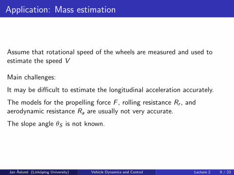
Application: Mass estimation

Assume that rotational speed of the wheels are measured and used toestimate the speed V

Main challenges:

It may be difficult to estimate the longitudinal acceleration accurately.

The models for the propelling force F , rolling resistance Rr , andaerodynamic resistance Ra are usually not very accurate.

The slope angle θS is not known.


Application: Mass estimation

Assume that the signal from an accelerometer, measuring the longitudinalacceleration, is available. How can this information be used?

The longitudinal equation of motion

ma = F − Rr − Rg − Ra

can be rewritten as

m(a + g sin θ) = F − Rr − Ra

and the accelerometer is measuring

a + g sin θ

Hence, it is not necessary to know the slope angle θ.


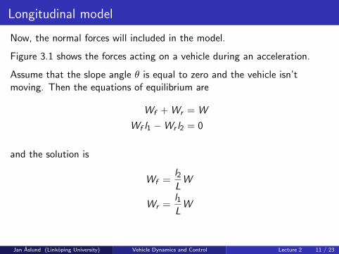
Longitudinal model

Now, the normal forces will included in the model.

Figure 3.1 shows the forces acting on a vehicle during an acceleration.

Assume that the slope angle θ is equal to zero and the vehicle isn’tmoving. Then the equations of equilibrium are

Wf + Wr = W

Wf l1 −Wr l2 = 0

and the solution is

Wf =l2LW

Wr =l1LW


Figure 3.1


Longitudinal model

Now, a moving vehicle will be considered.

It will be assumed that ha = hd = h and equilibrium of moments abouttwo point the distance h above the points A and B gives the equations

−Wl2 + LWf + h(Ff − Rrf ) + h(Fr − Rrr ) = 0

Wl1 − LWr + h(Ff − Rrf ) + h(Fr − Rrr ) = 0

with the solutions

Wf =l2LW − h

L(F − Rr )

and

Wr =l1LW +

h

L(F − Rr )


Maximal acceleration

Assume that the car is rear-wheel driven. What is the maximal propellingforce that is possible to accomplish? The limit case is

Fmax = µWr + frWr = (µ+ fr )

(l1LW +

h

L(Fmax − Rr )

)Solve for Fmax and use Rr = frW

Fmax =(µ+ fr )W (l1 − frh)

L− (µ+ fr )h

The corresponding result for a front-wheel driven car is

Fmax = (µ+ fr )Wf = (µ+ fr )

(l2LW − h

L(Fmax − Rr )

)och

Fmax =(µ+ fr )W (l2 + frh)

L + (µ+ fr )h


Lateral forces and stability: Introduction

Assume that a car is moving on a straight line and the motion is perturbed:

Direction of motion

The figure shows that

Front wheels turns the car counterclockwise (bad!?)

Rear wheel turns the car clockwise (good!?)


Lateral forces and stability: Braking

Assume that the rear wheels are used for braking causing a wheel lock-up:

Direction of motion

The figure shows that the car will turn away from the intended directionand the car will probably become unstable.


Lateral forces and stability: Braking

Let the front wheels be used instead causing a wheel lock-up:

Direction of motion

The figure shows that rear wheel turns the car towards the direction of theunperturbed direction. The drawback is that it becomes difficult tomaneuver the car.


Brake force distribution

The objective is to distribute the forces so that the front and rear begin toslide at the same time. Given a braking force Fb, we will find coefficientsKbf and Kbr , Kbf + Kbr = 1, and distribute the braking force Fbf = Kbf Fband Fbr = KbrFb to reach the objective.Figure 3.47 shows the forces acting on the vehicle

In this case we get

Wf =1

L(Wl2 + h(Fb + frW ))

och

Wr =1

L(Wl1 − h(Fb + frW ))


Figure 3.47


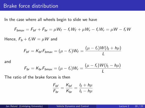
Brake force distribution

In the case where all wheels begin to slide we have

Fbmax = Fbf + Fbr = µWf − frWf + µWr − frWr = µW − frW

Hence, Fb + frW = µW and

Fbf = Kbf Fbmax = (µ− fr )Wf =(µ− fr )W (l2 + hµ)

L

and

Fbr = KbrFbmax = (µ− fr )Wr =(µ− fr )W (l1 − hµ)

L

The ratio of the brake forces is then

FbfFbr

=Kbf

Kbr=

l2 + hµ

l1 − hµ


Brake force distribution: Alternative approach

Assume now that brake force distribution is given, i.e., Kbf and Kbr whereKbf + Kbr = 1. Will the front or the rear wheel lock first?

Only the brake force and rolling resistance will be considered in this case.Hence

ma = Fb + Fr and Fb + frW =W

ga,

First, the front wheels will be considered. The normal force is

Wf =W

L

(l2 +

a

gh

),

In this case the brake force is

Fbf = Kbf Fb = KbfW

(a

g− fr

)



The front wheel will lock when

Fbf = µWf − frWf = (µ− fr )W

L

(l2 +

a

gh

)It follows that

KbfW

(a

g− fr

)=

(µ− fr )W

L

(l2 +

a

gh

)and the front wheels lock when(

a

g

)f

=(µ− fr )l2/L + Kbf frKbf − (µ− fr )h/L

In the same way wed get that the rear wheels lock when(a

g

)r

=(µ− fr )l1/L + Kbr frKbr + (µ− fr )h/L



Given a brake force distribution.

The front wheels will lock first if(a

g

)f

<

(a

g

)r

and the rear wheels will lock first if(a

g

)r

<

(a

g

)f


Documents

Vehicle Dynamics and Control · Vehicle Dynamics and Control Jan Aslund [email protected] Associate Professor Dept. Electrical Engineering Vehicular Systems Link oping University