Longitudinal vehicle dynamics control for improved vehicle safety

Herman A. Hamersma ⇑, P. Schalk Els

Department of Mechanical and Aeronautical Engineering, University of Pretoria, South Africa

Abstract

The aim is to investigate the improvements in vehicle safety that can be achieved by limiting the vehicle speed based on GPS pathinformation. The control strategy is aimed at reducing vehicle speed before a potentially dangerous situation is reached, in contrastwith widely used stability control systems that only react once loss of control by the driver is imminent. An MSC.ADAMS/Viewsimulation model of an off-road test vehicle was developed and validated experimentally. A longitudinal speed control system wasdeveloped by generating a reference speed based on the path information. This reference speed was formulated by taking intoaccount the vehicle’s limits due to lateral acceleration, combined lateral and longitudinal acceleration and the vehicle’s performancecapabilities. The model was used to evaluate the performance of the control system on various tracks. The control system was imple-mented on the test vehicle and the performance was evaluated by conducting field tests. Results of the field tests indicated that thecontrol system limited the acceleration vector of the vehicle’s centre of gravity to prescribed limits, as predicted by the simulations,thereby decreasing the possibility of accidents caused by rollover or loss of directional control due to entering curves at inappropri-ately high speeds.

Keywords: Autonomous vehicles; Vehicle safety; Vehicle modelling; Path planning; Off-road vehicles

1. Introduction

Applications of automation in vehicle engineering rangefrom rain sensing windscreen wipers to climate control sys-tems. More specific to the study of vehicle dynamics is theimprovement achievable by implementing feedback controlsystems which influence the dynamic behaviour of the vehi-cle with regards to the six degrees of freedom, namely lat-eral, vertical and longitudinal translation as well as roll,pitch and yaw rotation. Application of automation to con-trol these degrees of freedom may lead to the optimisationof vehicle utilisation.

⇑ Corresponding author.E-mail addresses: hhamersma@gmail.com (H.A. Hamersma), schalk.

els@up.ac.za (P.S. Els).

1.1. Fully autonomous vehicles

One of the best examples of the application of automa-tion in the modern engineering fraternity was during the2005 DARPA Grand Challenge [1] and the 2007 DARPAUrban Challenge [2]. Both these Challenges required vehi-cles to negotiate terrains that represent everyday drivingconditions (especially from a military point of view) andhence path planning played an important role in success-fully completing these Challenges. The 2005 DARPAGrand Challenge was won by Stanford University’s ‘Stan-ley’ [1] and the 2007 DARPA Urban Challenge was won by‘Boss’, the entry from Carnegie Mellon University, GeneralMotors, Caterpillar, Continental and Intel [2]. ‘Stanley’managed an average speed of 30.7 km/h [1] and ‘Boss’ anaverage speed of 22.5 km/h [2]. Due to the fairly low speedsinvolved, most DARPA Challenge entries employed simple

Nomenclature

Symbol DescriptionABrakes acceleration due to braking (m/s2)Af projected frontal area (m2)Amaxlong maximum allowed longitudinal acceleration

(m/s2)Ax acceleration in the x-direction (longitudinal)

(m/s2)Ay acceleration in the y-direction (lateral) (m/s2)Bj linear coefficient matrix of quadratic cost func-

tion for minimum curvature formulation(Dimensionless)

CD coefficient of aerodynamic drag (Dimensionless)ci constant term of straight line describing perpen-

dicular bisector (m)dprev preview distance (m)e velocity error (m/s)FD demand force (N)FDrag Force due to aerodynamic drag (N)Frr force due to rolling resistance (N)Fincl force due to longitudinal road inclination (N)g gravitational acceleration (m/s2)h centre of gravity height (m)Hj hessian matrix of quadratic cost function for

minimum curvature formulation (Dimension-less)

i unit vector in x-direction (Dimensionless)j unit vector in y-direction (Dimensionless)KD PID derivative gain (Dimensionless)KI PID integral gain (Dimensionless)KP PID proportional gain (Dimensionless)M vehicle mass (kg)mi gradient of chord of ith segment of trajectory

(Dimensionless)m0i gradient of perpendicular bisector of chord of

ith segment of trajectory (Dimensionless)n engine speed (rpm)P position of vehicle on track (m)Phyd hydraulic brake line pressure (MPa)p00–p40 coefficients of 2D polynomial (Dimensionless)

R radius of curve (m)Dsi length of ith track segment (m)t time (s)T throttle position (%)TEBT engine brake torque (N m)TEngine engine torque (N m)tw track width (m)u PID controller output (Dimensionless)V vehicle speed (m/s)Vref reference speed (m/s)x coordinate x value (m)xl left edge (bound) of road’s x-coordinate (m)xq,i X-coordinate of centre point of chord of ith

segment of trajectory (m)xr right edge (bound) of road’s x-coordinate (m)xR,i X-coordinate of centre point of arc of ith

segment of trajectory (m)DXi change in x-distance of ith track segment (m)y coordinate y value (m)yl left edge (bound) of road’s y-coordinate (m)yq,i Y-coordinate of centre point of chord of ith

segment of trajectory (m)yr right edge (bound) of road’s y-coordinate (m)yR,i Y-coordinate of centre point of arc of ith

segment of trajectory (m)Dyi change in y-distance of ith track segment (m)a parameter identifying position of vehicle on the

road (Dimensionless)aj parameter identifying position of vehicle on the

road for minimum curvature formulation(Dimensionless)

h inclination angle (radians)j curvature of trajectory (Dimensionless)l tyre-road friction coefficient (Dimensionless)lrr coefficient of rolling resistance (Dimensionless)q density of air (kg/m3)s preview time (s)

linear vehicle models to control speed and steering. A pos-sible area of improvement is thus to increase the speedthese vehicles attained while competing in the variousDARPA Challenges.

1.2. Driver assist systems

While the DARPA Challenges specifically aimed atdeveloping fully autonomous vehicles (vehicles that drivewith no human input), a more practical and feasibleapproach would be to develop a control system that canbe used as a driver aid. By using sensor technology similarto that employed in the DARPA Challenges (such as

numerous LIDARs, Differential GPS, radar and cameras),the vehicle can obtain preview information of its immediatesurroundings that enables it to identify a suitable path tobe followed. This is often referred to as path planning. Thispath information can subsequently be used for path follow-ing where decisions can be made that improve the vehicle’ssafety. Path planning using technology such as cameras,radar and LIDAR. has been extensively studied. This tech-nology is well commercialised and many vehicles are nowfitted with adaptive cruise control, traffic sign recognition,lane departure warning and satellite navigation. All thesetechnologies rely on camera, GPS and radar sensors. Inthe present study, this is not the contribution to be made.

The emphasis rather falls on developing a control systemthat uses information available from these sensors toenhance vehicle safety.

Many off-road vehicles are also used on roads. Due totheir high CG and suspension characteristics being opti-mised for off-road use, the handling and rollover propen-sity of these vehicles cause safety concerns when driven athigher speeds on roads. Several commercially availabletechnologies exist to help control the vehicle under impend-ing accident conditions. These include anti-lock brake sys-tems (ABS), electronic stability control (ESC), electronicbrake distribution (EBD) and active steering. These sys-tems however only start acting under extreme conditionswhere the driver and vehicle may already be in trouble.Path following algorithms that take vehicle dynamics andpath preview information into account may prevent thevehicle entering a situation where the handling can becomeunsafe, i.e. before ABS or ESC becomes active. The pro-posed system thus acts proactive rather than reactive. Inmany high-end vehicles all the required path previewinformation is already available as are the actuationsystems for steering and braking. The proposed controlsystem therefore does not require any additional hardware– it is simply a new software algorithm that improves avehicle’s safety. Table 1 shows a list of ‘Commercially offthe shelf’ (COTS) sensors, algorithms and interferencetechniques available. The focus of this research falls inthe column titled ‘Algorithms’.

1.3. Research question and focus of current paper

The research question of this paper may thus be definedas: to develop a longitudinal control system for path plan-ning and following that takes into account the nonlinearvehicle dynamics and uses GPS information for path pre-view. This control system should intelligently limit the vehi-cle’s speed to prevent the vehicle from exceeding the limitsimposed by the vehicle dynamics (i.e. rollover, sliding orovershooting the path) and hence improve the safety ofthe occupants. The control system is based on trajectoryplanning algorithm developed by Braghin et al. [3]. Braghinet al. [3] developed a similar control system and evaluated

Table 1List of COTS sensors, algorithms and interference techniques.

Path informationavailable

Algorithms Interference techniquesavailable

GPS or satellitenavigation

Adaptive cruisecontrol

Electronic power steering

Vehicle speed Lane departurewarning

Automated parking

Radar Blind spot warning ABSCameras High speed path

followingEBD

ESCActive or semi-activesuspension controlTorque vectoring

its performance with a simplified dynamic model. Theresults reported by [3] indicated that developing a controlsystem based on optimising the path of a vehicle may resultin improved lap times for race drivers. The same approachis followed in this paper but now with the focus on reduc-ing lateral acceleration of the vehicle and hence improvingvehicle safety rather than decreasing lap time around aracetrack.

A 1997 Land Rover Defender 300Tdi 110 Wagon is theexperimental platform used for this study. Feedback con-trol systems, that can mimic the inputs given by a humandriver, have been implemented in such a way that the testvehicle may be driven manually or via a computer. Severaldriver assist systems that lie somewhere between no controland fully autonomous control, such as an Anti-LockBraking System (ABS) and Traction Control, can beimplemented on the Land Rover test vehicle. The systemsimplemented on the vehicle consist of:

� A path following steering control system capable offully autonomous control up to high accelerationlimits.

� A braking control system.� A gear-shift and clutch control system.� A throttle pedal control system.

A model-based design approach is followed to developthe longitudinal control system and an experimentally val-idated model is thus required. An existing MSC.ADAMS/View multi-body dynamics model that accurately capturesthe fully nonlinear vertical and lateral dynamics of the testvehicle has been developed by Uys et al. [4]. The model isnow expanded and experimentally validated to accuratelycapture the longitudinal dynamics.

The driver models developed by Botha [5] have beenupdated and improved to provide for a trajectory planningalgorithm, based on the work done by Braghin et al. [3].The longitudinal control system is developed in simulationand finally validated experimentally.

2. ADAMS model development and validation

The acceleration and braking performance, aerody-namic drag and rolling resistance of the Land Rover testvehicle had to be characterised experimentally before inclu-sion in the existing MSC.ADAMS/View model of the LandRover.

2.1. Acceleration performance

The torque delivered by the engine is a function of twoparameters, namely engine speed and throttle position. Todetermine the torque delivered by the engine, strain gaugeswere applied to both forward and rearward drive shafts in afull-bridge configuration. The strain gauges were calibratedin the laboratory for direct torque measurement by apply-ing known torque values. The torque applied at a constant

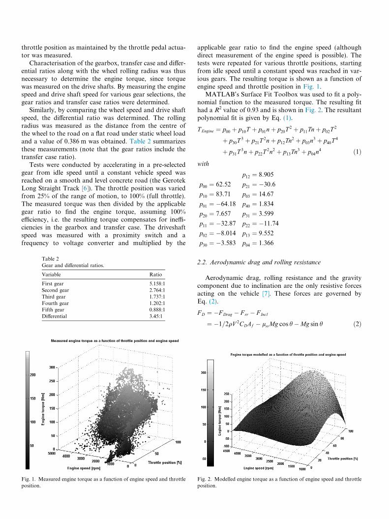
throttle position as maintained by the throttle pedal actua-tor was measured.

Characterisation of the gearbox, transfer case and differ-ential ratios along with the wheel rolling radius was thusnecessary to determine the engine torque, since torquewas measured on the drive shafts. By measuring the enginespeed and drive shaft speed for various gear selections, thegear ratios and transfer case ratios were determined.

Similarly, by comparing the wheel speed and drive shaftspeed, the differential ratio was determined. The rollingradius was measured as the distance from the centre ofthe wheel to the road on a flat road under static wheel loadand a value of 0.386 m was obtained. Table 2 summarizesthese measurements (note that the gear ratios include thetransfer case ratio).

Tests were conducted by accelerating in a pre-selectedgear from idle speed until a constant vehicle speed wasreached on a smooth and level concrete road (the GerotekLong Straight Track [6]). The throttle position was variedfrom 25% of the range of motion, to 100% (full throttle).The measured torque was then divided by the applicablegear ratio to find the engine torque, assuming 100%efficiency, i.e. the resulting torque compensates for ineffi-ciencies in the gearbox and transfer case. The driveshaftspeed was measured with a proximity switch and afrequency to voltage converter and multiplied by the

Table 2Gear and differential ratios.

Variable Ratio

First gear 5.158:1Second gear 2.764:1Third gear 1.737:1Fourth gear 1.202:1Fifth gear 0.888:1Differential 3.45:1

Fig. 1. Measured engine torque as a function of engine speed and throttleposition.

applicable gear ratio to find the engine speed (althoughdirect measurement of the engine speed is possible). Thetests were repeated for various throttle positions, startingfrom idle speed until a constant speed was reached in var-ious gears. The resulting torque is shown as a function ofengine speed and throttle position in Fig. 1.

MATLAB’s Surface Fit Toolbox was used to fit a poly-nomial function to the measured torque. The resulting fithad a R2 value of 0.93 and is shown in Fig. 2. The resultantpolynomial fit is given by Eq. (1).

T Engine ¼ p00 þ p10T þ p01nþ p20T 2 þ p11Tnþ p02T 2

þ p30T 3 þ p21T 2nþ p12Tn2 þ p03n3 þ p40T 4

þ p31T 3nþ p22T 2n2 þ p13Tn3 þ p04n4 ð1Þ

with

p12 ¼ 8:905

p00 ¼ 62:52 p21 ¼ �30:6

p10 ¼ 83:71 p03 ¼ 14:67

p01 ¼ �64:18 p40 ¼ 1:834

p20 ¼ 7:657 p31 ¼ 3:599

p11 ¼ �32:87 p22 ¼ �11:74

p02 ¼ �8:014 p13 ¼ 9:552

p30 ¼ �3:583 p04 ¼ 1:366

2.2. Aerodynamic drag and rolling resistance

Aerodynamic drag, rolling resistance and the gravitycomponent due to inclination are the only resistive forcesacting on the vehicle [7]. These forces are governed byEq. (2).

F D ¼ �F Drag � F rr � F Incl

¼ �1=2qV 2CDAf � lrrMg cos h�Mg sin h ð2Þ

Fig. 2. Modelled engine torque as a function of engine speed and throttleposition.

Fig. 4. Demand force due to drag and rolling resistance as a function ofvehicle speed.

The resistive forces due to drag and rolling resistancewere determined by accelerating the vehicle to 100 km/hand then coasting with the manual gearbox in neutral toa standstill on a level road while measuring the vehiclespeed. Fig. 3(a) presents the vehicle speed as a functionof time. The vehicle speed is differentiated to find accelera-tion and plotted in Fig. 3(b) as a function of time. ApplyingNewton’s Second Law the resistive force is calculated fromthe acceleration. The demand force is shown as a functionof vehicle speed in Fig. 4.

As may be seen from Eq. (2), the demand forces due todrag and rolling resistance (which in this case includesdrivetrain drag and other losses) are a function of vehiclespeed squared and a constant. A fit of this form was madethrough the captured data, resulting in the following coef-ficients (see Fig. 4):

qCDAf ¼ 2:583 ð3Þlrr ¼ 0:024 ð4Þ

2.3. Braking

In addition to the demand forces acting on the vehicle,the vehicle speed can be reduced by applying the vehicle’shydraulically actuated friction brakes or by engine braking.The friction brakes were characterised by accelerating thevehicle to 70 km/h and then braking to standstill whilemeasuring the longitudinal acceleration and the brake linehydraulic pressure. Fig. 5 shows that a linear relationship(given by Eq. (5)) exists between brake line pressure anddeceleration. Multiplying the deceleration with the vehiclemass gives the braking force.

ABrakes ¼ 0:832P hyd � 0:5507 ð5ÞThe engine braking torque is applied to the power train

when the driver removes his/her foot from the throttlepedal while the vehicle is moving and in gear. This is due

Fig. 3. Coast down experimental results.

Fig. 5. Longitudinal deceleration as a function of brake line hydraulicpressure.

to the torque required to turn the engine while compressingthe air inside the cylinders. This torque is multiplied by allthe gear, transfer case and differential ratios that form partof the vehicle’s power train and is applied to the drivingwheels. Characterisation of the engine braking torquewas done by Botha [8]. The measured characteristic is givenin Fig. 6 and the governing equation is given by Eq. (6).

T EBT ¼ 3:8713� 10�6n2 � 25:11� 10�3nþ 5:44 ð6Þ

2.4. Model validation

The relationships developed in Sections 2.1–2.3 had tobe incorporated in the MSC.ADAMS/View model byusing co-simulation with MATLAB/Simulink. Fig. 7

Fig. 6. Engine braking torque as a function of engine speed.

Fig. 8. Comparison of measured and modelled vehicle speeds forvalidation run.

shows a block diagram of the longitudinal model. The vari-ables calculated by the simulation model are vehicle speedand driveshaft speed. The control inputs given are thethrottle position, brake line pressure and the gear selected.These measured variables and control inputs are used todetermine the driveshaft torque (i.e. supply force) anddemand force acting on the vehicle.

A validation run was done with the Land Rover Defen-der while recording the vehicle’s speed, throttle pedal posi-tion, brake line hydraulic pressure and clutch pedalposition. The validation run consisted of four stages asindicated in Fig. 8:

Stage I. Accelerating from a standing start in first, sec-ond and third gear to 60 km/h (from 0 toapproximately 15 s).

Fig. 7. Schematic layout of mathematical l

Stage II. Decelerating with engine braking in third gearfrom 60 km/h back to idle speed (from approx-imately 15 s to just before 30 s).

Stage III. Accelerating in third and fourth gear from thirdgear idle speed up to 90 km/h (from 30 s toapproximately 55 s).

Stage IV. Braking with the clutch disengaged (from 55 sonwards).

The measured throttle pedal position and brake linepressure were used as inputs to the mathematical model.The gear change timing was accomplished by manuallyselecting the time (using MATLAB’s ‘ginput’ function) atwhich the clutch pedal was depressed and incrementingthe gear selection at each point.

ongitudinal model of the Land Rover.

The resulting speed, as calculated by the model is com-pared with the measured speed in Fig. 8. Fig. 9 shows thetorque applied to the driveshaft during the validation run.As may be seen from Fig. 8 there are some discrepanciespresent when comparing the modelled speed and measuredspeed of the vehicle. These errors may be attributed to:

(1) Inaccurate gear change timing.(2) The validation run was conducted on a slight down-

hill and the model does not provide for the effect ofthe component of gravity along an incline (althoughEq. (2) provides for the force component due to lon-gitudinal inclination but it was not implemented inthe model).

(3) There may have been external contributing factors(such as wind loading) that were not measured andnot accounted for in the model.

However, despite these discrepancies, a very close corre-lation may be seen for both vehicle speed and driveshafttorque in Figs. 8 and 9. Although several improvementsand refinements are possible, the model is deemed validatedand accurate enough for the current investigation.

3. Control system development

A common problem with sports-utility-vehicles is thelow rollover threshold, due to a high centre of gravity.The quasi-static rollover threshold is given by Eq. (7) [7]:

Ay

g¼ tw

2hð7Þ

Similarly, for a simple vehicle model, the vehicle willstart sliding when Ay P lg [7]. The lateral accelerationexperienced by a vehicle when negotiating a corner is givenby Eq. (8) [7]. Eq. (8) is derived for steady-state cornering(where the vehicle is traveling at a constant speed and

Fig. 9. Measured and modelled driveshaft torque for the validation run.

constant yaw rate). The method of reducing the vehicle’srollover propensity investigated by this project is to reducethe lateral acceleration experienced by the vehicle by eitherby reducing the speed or increasing the turn radius, ratherthan changing the rollover threshold.

Ay ¼V 2

Rð8Þ

From Eq. (8) it may be seen that by increasing the radiusof the corner being negotiated, the lateral acceleration willbe reduced and the speed at which rollover will occur iscorrespondingly increased, hence the development of a tra-jectory planning algorithm that maximises the radius ofcurvature. Although Eq. (8) is developed for steady-statecornering – which may not necessarily be the case duringdriving – it was assumed that the use of Eq. (8) is sufficientfor the purpose of this investigation. The use of an optimi-sation algorithm to determine the minimum curvature mayalso result in a “smoother” route, reducing the effect oftransient cornering.

The lateral acceleration limit at which sliding or rolloverwill occur depends on the terrain. While determining a suit-able acceleration limit as a function of the terrain is outsidethe scope of this study, there are several methods that canbe used, such as:

� Friction coefficient estimation through parameterestimation.

� Using side slope information (this may significantlyreduce the lateral acceleration at which rollover orsliding may occur).

� Driver input by selecting the type of terrain (e.g. sandor mud) or driver aid input (through a terrainresponse algorithm).

The idea is thus to, based on information received fromsensors such as GPS and radar, determine a suitable vehiclespeed to keep the longitudinal and lateral acceleration ofthe vehicle below prescribed limits to keep the vehicle safe.This reduction in speed must be sufficient to prevent elec-tronic stability control from being activated. The focus isalso not on path planning but rather on the vehicle dynam-ics required to follow a path safely.

3.1. Trajectory planning using minimum curvature approach

The roads or tracks used for simulation and experimentalpurposes are defined using GPS coordinates (latitude andlongitude), which can be converted to x and y coordinatesof the road centreline. By specifying the road width, the roadboundaries may also be determined. Trajectory planning isconcerned with determining the path the vehicle must followwhen negotiating a specified road or track. The trajectorymay be optimised for various operating conditions. Braghinet al. [3] developed two such methods – optimising for theshortest route and optimising for the minimum curvature.The minimum curvature formulation is applicable for the

Fig. 10. Minimised curvature trajectory of Geroteks ride and handlingtrack [6].

case under investigation, wherein minimising the curvatureof the path followed by the vehicle will result in maximizingthe radius of the trajectory and hence lowering the lateralacceleration (see Eq. (8)).

The approaches followed by Braghin et al. [3] rely ondiscretizing the road into segments. Given the road’s centr-eline coordinates, the left and right edges (or boundaries)of the road is then determined by assuming a track width(or using the actual measured track width). The positionof the vehicle on the road (which must lie within thebounds of the road) is then given by Eq. (9), where theposition depends on the variable a (which is allowed tovary between zero and unity, zero resulting in the positionbeing on the right boundary and unity on the left bound-ary) [3]:

P ¼ xr þ aðxl � xr Þiþ yr þ aðyl � yr Þj ð9ÞBraghin et al. [3] then formulates a bound quadratic

optimisation problem which, depending on the formula-tion, results in the shortest distance or minimum curvaturetrajectory, with a being the independent variable to be opti-mised. The cost function of the quadratic optimisationproblem for the shortest distance trajectory is formulatedfrom the distance formula in Cartesian coordinates and isgiven by Eq. (10).

j2 ¼ 1

2haji½Hj�fajg þ Bjfajg ð10Þ

Using MATLAB’s quadratic optimisation function, thetrajectory’s curvature is minimised. Fig. 10 shows the tra-jectory as optimised for Gerotek’s ride and handling track[6].

Systems such as satellite navigation and lane departurewarning system are readily available in the commercialvehicle market. Driver assist systems such as these maybe used to augment the trajectory planning methodsproposed by Braghin et al. [3]. A commercial GPS (witha typical accuracy of 15 m that updates its position approx-imately once per second [9] may be used in conjunctionwith a satellite navigation system, such as described byDork [10], to determine the vehicle’s whereabouts on amap and what lies ahead, in essence determine the centre-line of the road or track the vehicle is negotiating. LaneDeparture Warning Systems, such as developed by Bataviaet al. [11], are now commercially available and may be usedto detect the road boundaries and the vehicle’s position rel-ative to the road boundaries. With knowledge of the roadcentreline from the satellite navigation system and the vehi-cle’s position relative to the road boundaries, vehicle tovehicle communication (V2V) or radar information, trajec-tory planning may readily be implemented in commercialvehicles using existing sensors.

3.2. Speed profile

Once the minimum curvature trajectory has been deter-mined, a reference speed at which the vehicle will attempt

to negotiate the track must be determined. This speed islimited by three factors, namely:

� Lateral acceleration limit.� Tyre contact force limit when longitudinal and lateral

acceleration is present.� The vehicle’s limitations with regards to longitudinal

acceleration and deceleration due to the engine and/orbraking system.

The process followed to formulate the speed profile isgiven schematically in Fig. 11.

3.2.1. Speed limit due to lateral acceleration

As is evident from Eq. (8), the speed limit due to lateralacceleration is a function of the radius of the trajectorybeing followed. An algorithm to determine the radius ofthe trajectory for each segment of the trajectory was devel-oped. Given three points, it is always possible to draw anarc with a constant radius that passes through all threepoints. The perpendicular bisectors of the chords joiningadjacent points pass through the centre of the arc. The dis-tance from the centre of the arc to any of the three pointsused is the radius of curvature. Fig. 12 shows the result ofthis procedure.

The mathematical operations needed to determine theradius of curvature following this procedure will now beexplained. First, the perpendicular bisectors are deter-mined. The bisectors are located at the centre of eachchord, thus the centre points of each chord have to bedetermined:

xq;i ¼1

2ðxi þ xiþ1Þ ð11Þ

yq;i ¼1

2ðyi þ yiþ1Þ ð12Þ

Fig. 11. Flowchart describing formulation of speed profile.

Fig. 12. Constructing an arc through three points.

The line bisecting the chord from the two adjacent pointsis perpendicular to the chord, hence the product of the slopeof the chord “line” and the slope of the “bisector” line mustbe negative one. The gradient of the chord is thus deter-mined and used to determine the gradient of the bisector:

mi ¼Dyi

Dxi¼ yiþ1 � yi

xiþ1 � xið13Þ

The bisector’s gradient is given by Eq. (14):

m0i ¼�1

mið14Þ

Finally the constant term describing the straight lineequation of the bisector is determined. Since it is knownthat the bisector passes through the point (xq,i; yq,i), theconstant term is calculated with:

ci ¼ yq;i � m0ixq;i ð15Þ

The centre point of the arc is then at the intersection ofthe two bisectors, given by Eqs. (16) and (17):

xR;i ¼ciþ1 � ci

m0i � m0iþ1

ð16Þ

yR;i ¼ m0ixR;i þ ci ð17Þ

The radius of the arc (and hence the radius of curvature)is then determined with Pythagoras’ theorem:

Ri ¼ffiffiffiffiffiffiffiffiffiffiffiffiffiffiffiffiffiffiffiffiffiffiffiffiffiffiffiffiffiffiffiffiffiffiffiffiffiffiffiffiffiffiffiffiffiffiffiffiðxR;i � xiÞ2 þ ðyR;i � yiÞ

2q

ð18Þ

Fig. 13(a) shows a spiral with a radius increasing fromzero to 50 m. The radius of curvature is confirmed withthe outlined algorithm. The radius as a function of arclength is also shown in Fig. 13(b). A slight discrepancybetween the true and calculated radius may be seen inFig. 13(b). This discrepancy is present right at the begin-ning of the spiral. A possible explanation is that the algo-rithm cannot calculate a radius of zero. The algorithmworks well for radii greater than 5 m and is thus more thanadequate for vehicle trajectory, since a vehicle’s turningradius is seldom less than 5 m.

This algorithm may now be used to determine the max-imum permissible speed for the vehicle around any track.By specifying a maximum lateral acceleration, the corre-sponding speed at which this acceleration will occur maybe calculated for each point on the trajectory. However,from Eq. (8) it may be seen that when the radius of the tra-jectory is large, the permissible speed is very high (in astraight line, there is no lateral acceleration) and hence aspeed limit of 130 km/h was imposed. This is approxi-mately the maximum speed the Land Rover can achieve.Fig. 14 shows the speed as limited by lateral accelerationfor the Land Rover around the Gerotek ride and handlingtrack [6]. A maximum lateral acceleration of 0.5 g was spec-ified in this case.

3.2.2. Speed limit due to friction circle and vehicle

performance

When accelerating a vehicle both longitudinally andlaterally simultaneously, one has to consider the frictioncircle. Since forces are being generated in two directionsin a highly nonlinear system, one cannot simply considereach load condition separately. In Section 3.2.1 the speed

Fig. 13. Spiral with radius increasing from zero to 50 m and radius of curve as a function of arc length.

profile around the track was optimised for maximumlateral acceleration and hence maximum lateral forcegeneration. The available friction thus limits the vehicle’slongitudinal performance. If the friction force is exceeded,the wheels would slip (spin or lock), which may result in anunstable and unsafe situation.

The friction available for longitudinal acceleration isthus governed by the friction circle. The friction forceavailable for longitudinal acceleration is the vector subtrac-tion of the developed lateral force from the friction forcelimit. This is determined with Eq. (19) [3]:

Ax;i ¼ Ax;max

ffiffiffiffiffiffiffiffiffiffiffiffiffiffiffiffiffiffiffiffiffiffiffiffiffiffiffiffiffiffiffiffiffiffi1� ðAy;i=Ay;maxÞ2

qð19Þ

By imposing a speed limit on the vehicle when negotiat-ing the track, the maximum longitudinal accelerationallowable may be determined. Considering the vehicle’slimitations in terms of performance and braking, onemay determine the distance required to accelerate anddecelerate the vehicle. The vehicle’s performance capabili-ties on a level road are shown as functions of vehicle speedin Fig. 15. Fig. 15(a) shows the maximum accelerationthrough the gears, Fig. 15(b) indicating the maximumbraking performance. These plots were determined fromthe experimental data, discussed in detail in Section 2.

3.2.3. Speed profile algorithmThe speed profile that will be used as the reference speed

to be maintained by the vehicle while negotiating theprescribed path is now determined by defining the maxi-mum lateral and longitudinal acceleration deemed safe. Apreview distance is defined as a function of the currentvehicle speed and the maximum allowable longitudinalacceleration; the function is given in Eq. (20).

dprev ¼ V s� 0:5Amaxlongs2 þ const ð20Þ

The maximum allowable safe speed as limited by the lat-eral acceleration of the vehicle (see Eq. (8)) for the path tobe followed from the current position to the preview pointis compared with the current speed of the vehicle. If theallowable speed is higher than the current vehicle speed,the vehicle is allowed to accelerate. The accelerationallowed is determined by taking the lesser of the accelera-tions due to the vehicle’s performance capability (seeFig. 15(a)) and the friction available at the current position(see Eq. (19)). The vehicle’s speed at the next position in thepath is then updated using the equations of motion assum-ing constant acceleration (see Eq. (21)):

V iþ1 ¼ffiffiffiffiffiffiffiffiffiffiffiffiffiffiffiffiffiffiffiffiffiffiffiffiffiV 2

i þ 2AxDsi

qð21Þ

Fig. 16 shows the reference speed for Gerotek’s ride andhandling track [6]. The solid line is the speed limit imposedby Eq. (8) but with the vehicle’s top speed of 130 km/himposed. The dashed line is the reference speed calculatedwith Eq. (21). It may be noted that the dashed line is neverhigher than the solid line, indicating that, if the control sys-tem tracks the reference speed accurately, the vehicle willnever exceed its lateral limits due to excessive speed. Thisis validated in Section 3.3.

3.3. ADAMS validation of speed profile

Before simulation could be performed, some basic con-trol strategies had to be developed to control the actuatorpositions. These control strategies control the throttlepedal position, the brake line hydraulic pressure and thegear selection that are used as input to the longitudinalspeed controller as indicated in Fig. 7. During testing onthe vehicle throttle pedal position, steering and gear selec-tion will be performed by the person driving the vehicle,while brake line pressure will be controlled by actuating apneumatic cylinder mounted to the brake pedal.

Fig. 14. Enlarged view of speed limit due to lateral acceleration 30 km h.

Fig. 15. Land Rover performance limits.

The vehicle acceleration was controlled by controllingthe throttle pedal position and brake line hydraulic pres-sure. The throttle pedal position was controlled with aPID controller and the brake line hydraulic pressure witha PI controller. The gains for these controllers were deter-mined on a trial-and-error basis. The details for of thesecontrollers are not the focus of this paper. The dynamicsof the controllers and the actuators are an order of magni-tude faster than the vehicle response and the controllergains have a small influence on the vehicle performance.

The velocity error is determined with Eq. (22), with thecontrol system distinguishing between a positive and a

negative error to determine whether acceleration or decel-eration of the vehicle is necessary. When the error causesthe vehicle to brake, the throttle position is immediatelyset to zero and vice versa. The control signals sent to thevehicle are the throttle pedal position and brake linehydraulic pressure.

e ¼ V ref � V ð22ÞThe gear selection is simply done by monitoring the

engine speed. If the engine speed is higher than3500 RPM the gear is incremented once (unless the vehicleis in top gear) and if the engine speed is less than1200 RPM the gear is decremented once (unless the vehicleis in first gear). Although this is not an optimum gearshifting regime (the ideal would be to change gears at theintersection of the supply curves in the various gears), thismethod of controlling the gear selection was chosen due toits simplicity and the ease with which such a feedbackcontrol system could be implemented in simulation. Onthe actual test vehicle the gear selection was done by thedriver.

The next step was to simulate the MSC.ADAMS/Viewmodel of the Land Rover’s response to the inputs gener-ated by the developed control system (which tracks the ref-erence speed profile). The result for negotiating GerotekTest Facilities’ [6] Ride and Handling Track is shown inFig. 17. It was assumed throughout that the track was flat.Fig. 17(a) shows a plan view of the track. Fig. 17(c) indi-cates the following: (i) the speed limited by Eq. (8) (solidblack line), (ii) the reference speed calculated from Eq.(21) (grey line) and (iii) the speed obtained by the vehicleas the MSC.ADAMS model tries to accelerate and brakethe vehicle in order to follow the reference speed.

Fig. 16. Reference speed for Geroteks ride and handling track.

Fig. 17. Simulation results for Geroteks ride and handling track (maximum lateral and longitudinal acceleration of 8 m/s2).

It may be noted that the simulated speed never exceedsthe reference speed but that it tracks the prescribed speedclosely. The acceleration of the vehicle is slower and there-fore cannot follow the prescribed speed. The vehicle doesbrake fast enough so as to keep the vehicle speed at orbelow the reference speed. The vehicle is thus underpow-ered and could drive the track faster with a more powerfulengine. The resultant longitudinal and lateral accelerationsare plotted in the Fig. 17(d) and the g–g diagram(Fig. 17(b)). The g–g diagram in (Fig. 17(b)) indicates thatthe vehicle largely stayed within the prescribed accelerationlimits (the dashed circle is the friction circle with longitudi-nal and lateral acceleration limits of 8 m/s2). The driver

model used during the simulations maintained control overthe vehicle at all times, even though the prescribed limitsare very close to the vehicle’s limits. The simulations wererepeated for several race tracks of which GPS coordinatesare available.

Simulation results indicate that the vehicle performs asplanned, tracking the reference speed profile closely (con-sidering the slow dynamics of a vehicle such as a LandRover Defender) and that the accelerations measuredlargely stay within the friction circle. Hence the develop-ment of the longitudinal control system was deemed tohave been successful. The next step in the process is exper-imental validation of the longitudinal control system.

4. Experimental validation

The measurement transducers used during the experi-mental validation were:

� An accelerometer at the centre of gravity (CG) of thetest vehicle to measure longitudinal and lateralacceleration.� A VBox III Differential GPS [12] to measure the vehi-

cle’s speed and GPS position.� A hydraulic pressure transducer to measure the brake

line hydraulic pressure.� A rotary potentiometer to measure the throttle position.

A PC/104 form factor embedded computer with a Dia-mond MM-AT-12-bit Analogue to Digital I/O Module [13]was used for data acquisition. Since the longitudinal con-trol is a very slow dynamic process, a sample frequency

Fig. 18. Recorded x and y coordinates

Fig. 19. Schematic layout

of 100 Hz was deemed sufficient for both data acquisitionand control.

The VBox III Differential GPS [12] is a data logging systemthat can log GPS data at 100 Hz. A Local Differential GPSBase station was used in conjunction with the VBox III toimprove the positional accuracy to within 100 mm. The samesystem was used by Botha [5] as positional input to hissteering controller with resounding success.

A laptop, connected to the PC/104 computer via a TCPnetwork, was used in conjunction with the PC/104 to obtainthe GPS coordinates and vehicle speed from the VBox III.The measured velocity and prescribed velocity were com-pared and a velocity error calculated. The velocity errorwas used to determine whether the brakes had to be appliedor not. The PC/104 computer was used to control the brakeactuator, generating an analogue output to control thebrake line pressure and the driver controlled the throttle,clutch, gear lever and steering. A corresponding prompt

of ISO 3888-11999 severe...change.

of experimental setup.

was given to the driver as an indication whether the brakeswere going to be applied or not so that the driver couldrelease the throttle and depress the clutch.

The only actuator used for experimental validation wasthe pneumatic actuator that controls the vehicle’s decelera-tion by braking. The decision to only make use of thebraking control system is that it is more representative of

Fig. 20. Brake actuator response to ram

Fig. 21. Double lane change with lateral and longi

the intended application of the developed driver assist sys-tem. The driver manually operated the throttle, clutch,gears and steering during the validation run. While usinga human driver rather than the fully autonomous controlsystems described in Section 1 may cause significant errorswith respect to the path following, this gives an indicationas to the robustness of the driver assist system. The

p (left) and parabolic (right) input.

tudinal limits of 5 m/s2 and 8 m/s2 respectively.

application of the brakes to prevent the driver from exceed-ing the lateral acceleration limits of the vehicle was deemedto be sufficient for validation. During the run a prompt wasdisplayed on a computer screen indicating whether thevehicle’s speed was too high or too low. If the brakes werebeing applied, the driver disengaged the clutch. This was toprevent the vehicle from stalling while performing the dou-ble lane change manoeuvre (this may happen if the enginespeed drops below idle speed due to the vehicle driving tooslowly for the selected gear).

4.1. Experimental procedure

For the purpose of experimental validation, a severedouble lane change manoeuvre (ISO 3888-1:1999 [14])was performed. The boundaries of the severe double lanechange were laid out with high visibility cones. The exper-imental procedure may be described as follows:

(1) Record the path to be driven by driving at low speedwith the GPS.

(2) Define the maximum allowable lateral and longitudi-nal acceleration.

(3) Calculate the speed profile, as discussed in Section 3.2(pre-processing).

(4) Perform the severe double lane change manoeuvre.

Fig. 22. Double lane change with lateral and longit

The GPS coordinates of the path to be driven arerecorded with the VBox III. These GPS coordinates areconverted to x and y coordinates (shown in Fig. 18) thatare then used to determine the speed profile. The speed pro-file is determined as a function of GPS position.

While negotiating the severe double lane change, thevehicle compares its current speed (as measured with theVBox III) with the prescribed speed at that position. Ifthe measured speed is below the prescribed speed, the vehi-cle is allowed to accelerate. The vehicle’s brakes are appliedif the measured speed is above the prescribed speed.

Fig. 19 shows a schematic description of the brake actu-ator setup and control system. The actuator system consistsof:

a. 200 bar, 10 l air accumulator, pressure regulators anda 10 bar, 2 l air receiver.

b. Proportional and on–off air valves.

The ability of the brake pressure actuator to supply thecorrect pressure to the brake system was verified by apply-ing ramp and parabolic requirements. Fig. 20 indicates theprescribed pressures as well as the measured pressures. Thebrake actuator and control system follows the requiredpressure with very good accuracy and is deemed suitablefor use in autonomous braking of the vehicle.

udinal limits of 7 m/s2 and 8 m/s2 respectively.

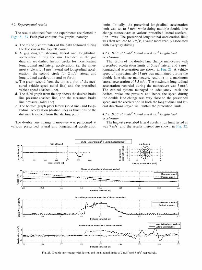
4.2. Experimental results

The results obtained from the experiments are plotted inFigs. 21–23. Each plot contains five graphs, namely:

a. The x and y coordinates of the path followed duringthe test run in the top left corner.

b. A g–g diagram showing lateral and longitudinalacceleration during the run. Included in the g–gdiagram are dashed friction circles for incrementinglongitudinal and lateral acceleration, i.e. the inner-most circle is for 1 m/s2 lateral and longitudinal accel-eration, the second circle for 2 m/s2 lateral andlongitudinal acceleration and so forth.

c. The graph second from the top is a plot of the mea-sured vehicle speed (solid line) and the prescribedvehicle speed (dashed line).

d. The third graph from the top shows the desired brakeline pressure (dashed line) and the measured brakeline pressure (solid line).

e. The bottom graph plots lateral (solid line) and longi-tudinal acceleration (dashed line) as functions of thedistance travelled from the starting point.

The double lane change manoeuvre was performed atvarious prescribed lateral and longitudinal acceleration

Fig. 23. Double lane change with lateral and longi

limits. Initially, the prescribed longitudinal accelerationlimit was set to 8 m/s2 while doing multiple double lanechange manoeuvres at various prescribed lateral accelera-tion limits. The prescribed longitudinal acceleration limitwas then reduced to 3 m/s2, a value more readily associatedwith everyday driving.

4.2.1. DLC at 5 m/s2 lateral and 8 m/s2 longitudinal

acceleration

The results of the double lane change manoeuvre withprescribed acceleration limits of 5 m/s2 lateral and 8 m/s2

longitudinal acceleration are shown in Fig. 21. A vehiclespeed of approximately 13 m/s was maintained during thedouble lane change manoeuvre, resulting in a maximumlateral acceleration of 3.5 m/s2. The maximum longitudinalacceleration recorded during the manoeuvre was 3 m/s2.The control system managed to adequately track thedesired brake line pressure and hence the speed duringthe double lane change was very close to the prescribedspeed and the acceleration in both the longitudinal and lat-eral directions stayed well within the prescribed limits.

4.2.2. DLC at 7 m/s2 lateral and 8 m/s2 longitudinal

acceleration

The highest prescribed lateral acceleration limit tested atwas 7 m/s2 and the results thereof are shown in Fig. 22.

tudinal limits of 3 m/s2 and 3 m/s2 respectively.

The maximum lateral and longitudinal accelerations mea-sured during the double lane change manoeuvre were4 m/s2 and 3.2 m/s2 respectively, well within the prescribedlimits. The double lane change was negotiated at 14 m/s,slightly lower than the speed as prescribed by the speed pro-file algorithm and hence the lateral acceleration was signif-icantly lower than the prescribed limit. The actuatorapplying the brakes adequately tracked the desired brakeline pressure, but the vehicle lost too much speed. Thismay be attributed to driver error, the driver neglecting tomaintain the speed once the double lane change had beenentered.

4.2.3. DLC at 3 m/s2 lateral and 3 m/s2 longitudinalacceleration

The prescribed longitudinal acceleration limit wasreduced to 3 m/s2, with the lateral acceleration limit at3 m/s2 and the experimental results are shown in Fig. 23.The reason for the low prescribed lateral acceleration limitis because the low prescribed longitudinal acceleration limitprevented the Land Rover from reaching a speed highenough to excite high lateral accelerations in the previoustests. During the double lane change, the maximum lateralacceleration measured was 2.8 m/s2 and the maximum lon-gitudinal acceleration 2 m/s2, the vehicle thus stayed withinthe prescribed acceleration limits. The double lanechange was negotiated at 10 m/s, similar to the speed inSection 4.2.1 which has the same prescribed lateral limit.

4.3. Discussion of results

During all of the double lane change manoeuvres per-formed the lateral acceleration of the vehicle was reducedas desired by controlling the longitudinal behaviour ofthe vehicle by braking. In all of the tests the measuredaccelerations never exceeded the prescribed limits. Thevehicle reduced speed when it exceeded the prescribedspeed, resulting in the measured accelerations being withinthe desired limits.

The pneumatic actuator used to control the vehicle’sbrakes adequately tracked the desired brake line pressurein all of the tests, even when noise was present. This vali-dated the design of the PID controller used to control thebrake line pressure.

The prescribed longitudinal acceleration limit was onlyreached when the prescribed limit was low. When the pre-scribed longitudinal acceleration was high, the vehiclebraked early, resulting in lower longitudinal accelerationsbeing measured. A possible explanation for this is thatthe preview distance used to determine when to apply thebrakes is too conservative, effectively looking too far aheadwhen the prescribed longitudinal acceleration is high.

5. Conclusions

The rollover risks of a vehicle (SUV) can be consider-ably reduced by controlling the maximum lateral

acceleration that the vehicle can achieve. Lateral acceler-ation can be limited by limiting the vehicle speed as afunction of turn radius. The trajectory of the track orroad to be followed was optimised to maximise the radiusof the path to be followed. This optimised trajectory wasused in conjunction with a longitudinal speed drivermodel to define a speed limit for the vehicle at each pointon the trajectory. The driver model took into accountprescribed longitudinal and lateral acceleration limitsand the vehicle’s lateral acceleration limits, the frictionavailable for combined longitudinal and lateral force gen-eration (due to the friction circle concept) and the vehi-cle’s longitudinal performance capabilities to formulatea safe speed at each point of the path being followed.These limits can be based on friction estimates, lookuptables (in response to an input from the driver tellingthe vehicle the nature of the terrain or from a terrainresponse system). The process of optimising the trajectoryand determining a safe speed was termed the speed profilealgorithm. A longitudinal control system was developedto control vehicle speed. The system aims to reduce vehi-cle speed early enough to prevent the vehicle from enter-ing a dangerous situation, i.e. it acts before electronicstability control (ESC) and similar driver assist systemsneed to start intervening.

The performance of the longitudinal control systemwas evaluated in simulation using the validated MSC.A-DAMS/View model of the Land Rover Defender. Severalracetracks of which the GPS coordinates are availablewere used for simulation purposes. A speed profile wasdeveloped for each racetrack and MSC.ADAMS/Viewwas used in conjunction with MATLAB and Simulinkto simulate the Land Rover Defender negotiating thesetracks. In all of the simulations, the steering controllermaintained control over the vehicle, even though themodel was operating very close to the vehicle’s limits.Throughout the simulations, the lateral and longitudinalaccelerations stayed within the prescribed limits. The sim-ulation results indicated that the longitudinal control sys-tem was safe for experimental validation on the LandRover Defender.

Experimental validation of the longitudinal controlsystem was done by performing an ISO 3888-1:1999severe double lane change manoeuvre. Speed profilesfor the double lane change were formulated with variousprescribed longitudinal and lateral acceleration limits.The pneumatic actuator used for controlling the brakeline pressure was used to prevent the vehicle fromexceeding the speed deemed safe by the speed profilealgorithm. During all the test runs, the vehicle’s mea-sured lateral and longitudinal accelerations were withinthe prescribed limits. The system was found to be conser-vative, rarely reaching the prescribed longitudinal accel-eration. The advantage of the system beingconservative is that it adds robustness to the speed pro-file algorithm, allowing it to be used for any prescribedacceleration limits.

6. Recommendations

Multiple aspects which could improve the longitudinalcontrol system and speed profile algorithm at higherprescribed acceleration limits have been identified. Theseinclude:

� The development of software that can optimise thetrajectory in real time, taking account of the vehi-cle’s current position, may result in a safer speedlimit being formulated.

� Additional sensors that may detect and can hencebe used to avoid obstacles may be integrated withthe system, e.g. lane departure warning systems.This may result in a more fully autonomous vehicle.

� By incorporating all the driver aids developed onthe Land Rover Defender, significant improve-ments in vehicle safety may be achieved. A strategyto decide when to employ which driver aid will needto be developed.

� Using parameter estimation techniques to estimatethe friction coefficient between the tyres and the ter-rain one may implement this control system onalmost any terrain and further improve the occu-pants’ safety.

Performing these recommendations may result in signif-icant improvements in the vehicle’s performance, safetyand stability.

References

[1] Thrun S. Winning the darpa grand challenge. In: Knowledgediscovery in databases: PKDD 2006. Berlin, Heidelberg: Springer;2006. p. 4-4.

[2] Urmson C, Anhalt J, Bagnell D, Baker C, Bittner R, Clark MN.Autonomous driving in urban environments: Boss and the urbanchallenge. J Field Robot 2008;25(8):425–66.

[3] Braghin F, Melzi S, Sabbioni E, Poerio N. Identification of theoptimal trajectory for a race driver. In: Proceedings of the ASME2011 international design engineering technical conferences & com-puters and information in engineering conference, 28–31 August2011. American Society of Mechanical Engineers, Washington, DC,USA; 2011.

[4] Uys PE, Els PS, Thoresson MJ. Suspension settings for optimal ridecomfort of off-road vehicles travelling on roads with differentroughness and speeds. J Terramech 2007;44:163–75.

[5] Botha TR. High speed autonomous off-road vehicle steering.MEng(Mechanical) thesis, University of Pretoria; 2011. <http://www.upetd.up.ac.za/thesis/available/etd-11212011-125411/>.

[6] Gerotek test facilities; 2013. <http://www.armscordi.com/SubSites/Gerotek1/Gerotek01_landing.asp> [accessed 12.03.13].

[7] Gillespie TD. Fundamentals of vehicle dynamics. Warrendale, PA:Society of Automotive Engineers; 1992.

[8] Botha TR. Brake control – autonomous vehicle brake system.Unpublished BEng(Mechanical) final year project, University ofPretoria; 2008.

[9] Garmin. What is GPS?; 2013. <http://www8.garmin.com/aboutGPS/> [accessed 18.07.13].

[10] Dork RA. Satellite navigation systems for land vehicles. IEEEAerospace Electr Syst Mag 1987;2(5):2–5.

[11] Batavia PH, Pomerlau DA, Thorpe CE. Predicting lane position forroadway departure prevention. In: Proceedings of the IEEE intelli-gent vehicles symposium; 1998

[12] Racelogic. VBOXTools software manual ver1.9; 2008. <http://www.racelogic.co.uk/_downloads/vbox/Manuals/Data_Loggers/RLVB3_Manual%20-%20English.pdf> [accessed 12.03.13].

[13] Diamond Systems Corporation. DIAMOND-MM-AT user manualV1.21. Diamond Systems Corporation, Newark, CA; 2004.

[14] International Organization for Standardization. ISO 3888-1:1999:passenger cars – test track for a severe lane-change manoeuvre – Part1: Double lane-change. Geneva, ISO; 1999.