Embed Size (px)
Citation preview
Vector Calculus
1 Line Integrals
Mass problem. Find the mass M of a very thin wire whose linear
density function (the mass per unit length) is known.
We model the wire by a smooth curve C between two points P and Q
in 3-space. Given any point (x, y, z) on C, we let f (x, y, z) denote the
corresponding value of the density function.
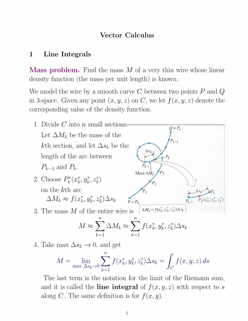
1. Divide C into n small sections.
Let ∆Mk be the mass of the
kth section, and let ∆sk be the
length of the arc between
Pk−1 and Pk.
2. Choose P ∗k (x∗k, y∗k, z∗k)
on the kth arc
∆Mk ≈ f (x∗k, y∗k, z∗k)∆sk
3. The mass M of the entire wire is
M ≈n∑k=1
∆Mk ≈n∑k=1
f (x∗k, y∗k, z∗k)∆sk
4. Take max ∆sk → 0, and get
M = limmax ∆sk→0
n∑k=1
f (x∗k, y∗k, z∗k)∆sk =
ˆC
f (x, y, z) ds
The last term is the notation for the limit of the Riemann sum,
and it is called the line integral of f (x, y, z) with respect to s
along C. The same definition is for f (x, y).
1

• The mass M of the wire is
M =
ˆC
f (x, y, z) ds
• The length L of the wire is
L =
ˆC
ds
• If C is a curve in the xy-plane and f (x, y) is nonnegative function
on C, then´C f (x, y) ds is equal to the area of the “sheet” that
is swept out by a vertical line segment that extends upward from
(x, y) to a height f (x, y) and moves along C
∆Ak ≈ f (x∗k, y∗k)∆sk ⇒ A =
ˆC
f (x, y) ds
2

Evaluating line integrals
Let C be smoothly parametrised
~r = x(t)~i + y(t)~j , a ≤ t ≤ b .
Then
∆sk =´ tktk−1|~r ′(t)|dt = |~r ′(t∗k)|∆tk
and
ˆC
f (x, y) ds = limmax ∆sk→0
n∑k=1
f (x∗k, y∗k)∆sk
= limmax ∆tk→0
n∑k=1
f (x(t∗k), y(t∗k))|~r ′(t∗k)|∆tk
=
ˆ b
a
f (x(t), y(t))|~r ′(t)| dt
=
ˆ b
a
f (x(t), y(t))
√(dx
dt
)2
+
(dy
dt
)2
dt
The line integral does not depend on a parametrisation of C,
in particular on an orientation of C.
Example. Find´C(1 + x2y)ds for
1. C : 12(t + t2)~i + 1
2(t + t2)~j , 0 ≤ t ≤ 1
2. C : (2− 2t)~i + (1− t)~j , 0 ≤ t ≤ 1
3
Similarly, if C is a curve in 3-space smoothly parametrised
~r = x(t)~i + y(t)~j + z(t)~k , then
ˆC
f (x, y, z) ds =
ˆ b
a
f (x(t), y(t), z(t))|~r ′(t)| dt
=
ˆ b
a
f (x(t), y(t), z(t))
√(dx
dt
)2
+
(dy
dt
)2
+
(dz
dt
)2
dt
Example. Find´C(xy + z3)ds for
C : cos t~i + sin t~j + t~k , 0 ≤ t ≤ π
Answer :√
2π4/4
Line integrals with respect to x, y and z
Let’s replace ∆sk by ∆xk ( or ∆yk or ∆zk) in the definition of the line
integral. Then, we get the line integral of f (x, y, z) with respect
to x along C
ˆC
f (x, y, z) dx = limmax ∆sk→0
n∑k=1
f (x∗k, y∗k, z∗k)∆xk
ˆC
f (x, y, z) dy = limmax ∆sk→0
n∑k=1
f (x∗k, y∗k, z∗k)∆yk
ˆC
f (x, y, z) dz = limmax ∆sk→0
n∑k=1
f (x∗k, y∗k, z∗k)∆zk
4
The sign of these line integrals depends on the orientation of C.
Reversing the orientation changes the sign.
Thus, one should find parametric equations for C in which
the orientation of C is in the direction of increasing t, and then
ˆC
f (x, y, z) dx =
ˆ b
a
f (x(t), y(t), z(t))x′(t) dt
Example. Find´C(1 + x2y)dy for
1. C : 12(t + t2)~i + 1
2(t + t2)~j , 0 ≤ t ≤ 1
2. C : (2− 2t)~i + (1− t)~j , 0 ≤ t ≤ 1
Let C be a smooth oriented curve, and let −C denote the oriented
curve with opposite orientation but the same points as C. Then
ˆC
f (x, y) dx = −ˆ−Cf (x, y) dx ,
ˆC
f (x, y) dy = −ˆ−Cf (x, y) dy
while ˆC
f (x, y) ds = +
ˆ−Cf (x, y) ds
Convention
ˆC
f (x, y) dx + g(x, y) dy =
ˆC
f (x, y) dx +
ˆC
g(x, y) dy
We have
ˆC
f (x, y) dx+g(x, y) dy =
ˆ b
a
(f (x(t), y(t))x′(t) + g(x(t), y(t)) y′(t)) dt
5

Integrating a vector field along a curve
Definition. A vector field in a plane is a function that associates
with each point P in the plane a unique vector ~F (P ) parallel to the
plane~F (P ) = ~F (x, y) = f (x, y)~i + g(x, y)~j
Similarly, a vector field in a 3-space is a function that associates with
each point P in the 3-space a unique vector ~F (P ) in the 3-space
~F (P ) = ~F (x, y, z) = f (x, y, z)~i + g(x, y, z)~j + h(x, y, z)~k
One can say that a vector field is a vector-valued function with the
number of components equal to the number of independent variables
(coordinates).
Introduce d~r = dx~i + dy~j + dz ~k
If ~F (x, y, z) = f (x, y, z)~i + g(x, y, z)~j + h(x, y, z)~k is a continuous
vector field, and C is a smooth oriented curve, then the line integral
of ~F along C is
ˆC
~F · d~r =
ˆC
(f~i + g~j + h~k) · (dx~i + dy~j + dz ~k)
=
ˆC
f (x, y, z) dx + g(x, y, z) dy + h(x, y, z) dz
If ~r = ~r(t) = x(t)~i + y(t)~j + z(t)~k, thenˆC
~F · d~r =
ˆ b
a
~F (~r(t)) · ~r ′(t) dt
6
Example.
The curve C is a line segment connecting the points (−π/2 , π) and
(3π/2 ,−2π/3). Parameterise C, and evaluateˆC
~F · d~r
where
~F (x, y) = (−6xy + 3π3 sin 3x)~i− (3x2 + 2π3 cos3y
2)~j
Answer :´C~F · d~r = 47
12π3 ≈ 121.441
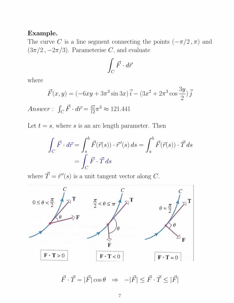
Let t = s, where s is an arc length parameter. Then
ˆC
~F · d~r =
ˆ b
a
~F (~r(s)) · ~r ′(s) ds =
ˆ b
a
~F (~r(s)) · ~T ds
=
ˆC
~F · ~T ds
where ~T = ~r ′(s) is a unit tangent vector along C.
~F · ~T = |~F | cos θ ⇒ −|~F | ≤ ~F · ~T ≤ |~F |
7

Line integrals along piecewise smooth curves
If C is a curve formed from finitely many
smooth curves C1, C2,..., Cn joined end to end,
then
ˆC
=
ˆC1
+
ˆC2
+ · · · +ˆCn
Example. Let the curve C between the points
(−π/2 , π) and (3π/2 ,−2π/3) be a curve
formed from two line segments C1 and C2,
where C1 is joining (−π/2 , π) and (3π/2 , π),
and C2 is joining (3π/2 , π) and (3π/2 ,−2π/3).
Parameterise C1 and C2, and evaluateˆC
~F · d~r
where
~F (x, y) = (−6xy + 3π3 sin 3x)~i− (3x2 + 2π3 cos3y
2)~j
8

2 Independence of path; Conservative vector fields
The curve C in´C~F · d~r is called the path of integration.
If ~F is conservative, i.e.
~F = ~∇φ =∂φ
∂x~i +
∂φ
∂y~j , or ~F = ~∇φ =
∂φ
∂x~i +
∂φ
∂y~j +
∂φ
∂z~k
then it depends only on the end points.
Example. ~F = y~i + x~j, a) y = x, b) y = x2, c) y = x3.
The Fundamental Theorem of Line Integrals
Let ~F (x, y) = f (x, y)~i+g(x, y)~j = ~∇φ(x, y) be a conservative vector
field in some open region D containing the points (x0, y0) and (x1, y1),
and let f (x, y) and g(x, y) be continuous in D. If C is any piecewise
smooth parametric curve that starts at (x0, y0), ends at (x1, y1), and
lies in D, then
ˆC
~F (x, y) · d~r = φ(x1, y1)− φ(x0, y0)
or, equivalently ˆC
~∇φ · d~r = φ(x1, y1)− φ(x0, y0)
Proof. Assume C is smooth for simplicityˆC
~∇φ · d~r =
ˆC
∂φ
∂xdx +
∂φ
∂ydy =
ˆ b
a
(∂φ
∂xx′(t) +
∂φ
∂yy′(t)
)dt
=
ˆ b
a
d
dt(φ(x(t), y(t))) dt = φ(x1, y1)− φ(x0, y0)
9

Line integrals along closed paths
If ~F is conservative, and C is closed then
ˆC
~F (x, y) · d~r = φ(~r(b))− φ(~r(a)) = 0
The converse of this result is also true.
If the line integral is 0 along all closed
paths then ~F = ~∇φ
Theorem. If f (x, y) and g(x, y) are continuous on some open con-
nected region D, then the following statements are equivalent
1. ~F (x, y) = f (x, y)~i + g(x, y)~j is a conservative vector field on D.
2.´C~F · d~r = 0 for every piecewise smooth closed curve C in D.
3.´C~F ·d~r is independent of the path from any point P in D to any
point Q in D for every piecewise smooth curve C in D.
Proof. We have proven 1→ 2.
Then, 2→ 3 is straightforward.
Finally, 3→ 1 is proven by
constructing φ(x, y)
φ(x, y) =
ˆ (x,y)
(a,b)
~F · d~r
10
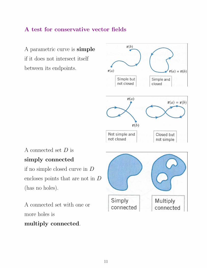
A test for conservative vector fields
A parametric curve is simple
if it does not intersect itself
between its endpoints.
A connected set D is
simply connected
if no simple closed curve in D
encloses points that are not in D
(has no holes).
A connected set with one or
more holes is
multiply connected.
11

Theorem. (Conservative Field Test)
If f (x, y) and g(x, y) have continuous first partial derivatives on some
open region D, and if the vector field ~F (x, y) = f (x, y)~i+ g(x, y)~j is
conservative on D, then
∂f
∂y=∂g
∂xat each point in D.
Conversely, if D is simply connected and fy = gx holds at each point
in D, then ~F (x, y) = f (x, y)~i + g(x, y)~j is conservative.
If~F = ~∇φ =
∂φ
∂x~i +
∂φ
∂y~j
then∂f
∂y=
∂
∂y
∂φ
∂x=
∂
∂x
∂φ
∂y=∂g
∂x
Example. Show that ~F is conservative, and find φ
~F (x, y) = (−6xy + 3π3 sin 3x)~i− (3x2 + 2π3 cos3y
2)~j
Conservative vector fields in 3-space
ˆC
~F (x, y, z) · d~r = φ(x1, y1, z1)− φ(x0, y0, z0)
Test.∂f
∂y=∂g
∂x,
∂f
∂z=∂h
∂x,
∂g
∂z=∂h
∂y
12
3 Green’s Theorem
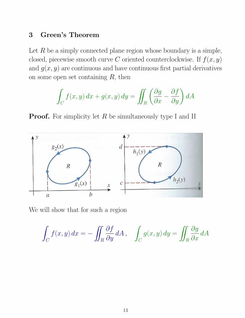
Let R be a simply connected plane region whose boundary is a simple,
closed, piecewise smooth curve C oriented counterclockwise. If f (x, y)
and g(x, y) are continuous and have continuous first partial derivatives
on some open set containing R, then
ˆC
f (x, y) dx + g(x, y) dy =
¨R
(∂g
∂x− ∂f
∂y
)dA
Proof. For simplicity let R be simultaneously type I and II
We will show that for such a region
ˆC
f (x, y) dx = −¨
R
∂f
∂ydA ,
ˆC
g(x, y) dy =
¨R
∂g
∂xdA
13

We have
ˆC
f (x, y) dx =
ˆC1
f (x, y) dx
+
ˆC2
f (x, y) dx
C1 : x = t , y = g1(t);
−C2 : x = t , y = g2(t);
Thus ˆC
f (x, y) dx =
ˆ b
a
f (t, g1(t)) dt−ˆ b
a
f (t, g2(t)) dt
= −ˆ b
a
[f (t, g2(t))− f (t, g1(t))] dt
= −ˆ b
a
ˆ g2(t)
g1(t)
∂f
∂y(t, y) dy dt = −
¨R
∂f
∂ydA
Notation for line integrals around simple closed curves˛C
f (x, y) dx + g(x, y) dy =
¨R
(∂g
∂x− ∂f
∂y
)dA
‰C
f (x, y) dx + g(x, y) dy =
¨R
(∂g
∂x− ∂f
∂y
)dA
C
f (x, y) dx + g(x, y) dy =
¨R
(∂f
∂y− ∂g
∂x
)dA
Example. Consider the integral (Answer : I = 163 )
I =
‰C
(e−2x + 5x2y − 2y2) dx− (3ey − 3x3) dy
C is the boundary of R between y = x2/2 and y = x.
14

Finding areas using Green’s theorem
A =
¨R
dA =⇒ ∂g
∂x− ∂f
∂y= 1
Simplest solutions
i) f = 0 , g = x =⇒ A =
‰C
x dy
ii) f = −y , g = 0 =⇒ A = −‰C
y dx
iii) f = −y2, g =
x
2=⇒ A =
1
2
‰C
−y dx + x dy
Example. Find A of x2/a2 + y2/b2 = 1
Green’s theorem for multiply connected regions
Positive orientation of R:
the outer boundary is
oriented counterclockwise
the inner boundaries
are oriented clockwise.
Divide R into two simply
connected regions R′ and R′′.
15
¨R
(∂g
∂x− ∂f
∂y
)dA =
¨R′
(∂g
∂x− ∂f
∂y
)dA +
¨R′′
(∂g
∂x− ∂f
∂y
)dA
=
‰
boundaryof R′
f (x, y) dx + g(x, y) dy +
‰
boundaryof R′′
f (x, y) dx + g(x, y) dy
=
‰C1
f (x, y) dx + g(x, y) dy +
C2
f (x, y) dx + g(x, y) dy
=
˛
boundaryof R
f (x, y) dx + g(x, y) dy
Example. Evaluate ‰C
−y dx + x dy
x2 + y2
if (a) C does not enclose the origin, and (b) C encloses the origin.
16
4 Surface Integrals
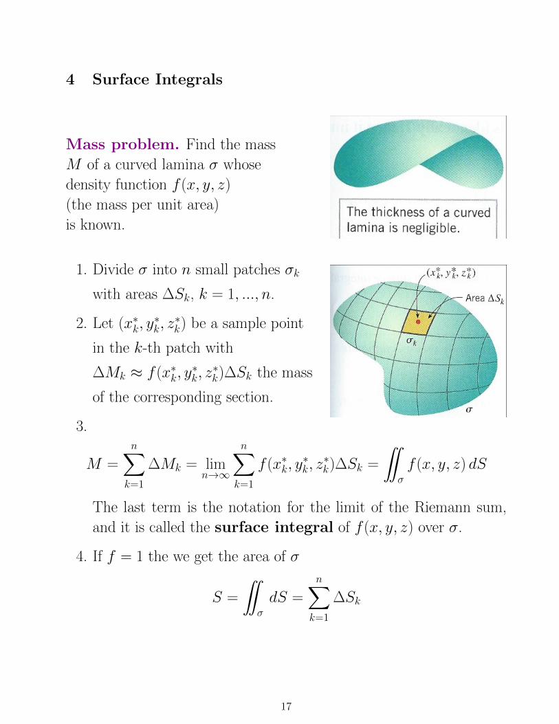
Mass problem. Find the mass
M of a curved lamina σ whose
density function f (x, y, z)
(the mass per unit area)
is known.
1. Divide σ into n small patches σk
with areas ∆Sk, k = 1, ..., n.
2. Let (x∗k, y∗k, z∗k) be a sample point
in the k-th patch with
∆Mk ≈ f (x∗k, y∗k, z∗k)∆Sk the mass
of the corresponding section.
3.
M =
n∑k=1
∆Mk = limn→∞
n∑k=1
f (x∗k, y∗k, z∗k)∆Sk =
¨σ
f (x, y, z) dS
The last term is the notation for the limit of the Riemann sum,
and it is called the surface integral of f (x, y, z) over σ.
4. If f = 1 the we get the area of σ
S =
¨σ
dS =
n∑k=1
∆Sk
17

Evaluating surface integrals
Theorem. Let σ be a smooth parametric surface whose vector equa-
tion is ~r = x(u, v)~i + y(u, v)~j + z(u, v)~k where (u, v) varies over a
region R in the uv-plane. If f (x, y, z) is continuous on σ, then
¨σ
f (x, y, z) dS =
¨R
f (x(u, v), y(u, v), z(u, v))
∣∣∣∣∂~r∂u × ∂~r
∂v
∣∣∣∣ dAThis formula follows by approximating ∆Sk as
∆Sk ≈∣∣∣∣∂~r∂u × ∂~r
∂v
∣∣∣∣∆Ak
Example. σ: x2 + y2 + z2 = 1.˜σ y
2 dS =? Answer : 4π/3.
Surface integrals over z = g(x, y), y = g(x, z), x = g(y, z)
If σ is a surface of the form z = g(x, y), we take
x = u , y = v ⇒ ~r = u~i + v~j + g(u, v)~k
∣∣∣∣∂~r∂u × ∂~r
∂v
∣∣∣∣ =
√1 +
(∂z
∂u
)2
+
(∂z
∂v
)2
⇒ (u→ x , v → y)
¨σ
f (x, y, z) dS =
¨R
f (x, y, g(x, y))
√1 +
(∂z
∂x
)2
+
(∂z
∂y
)2
dA
The region R lies in the xy-plane and is the projection of σ on the
xy-plane. Analogously for y = g(x, z), x = g(y, z).
18

Example. Find the mass of the lamina that is the portion of x2 +
y2 − 3z − 1 = 0 inside x2 + y2 = 9/4. The density is
δ(x, y, z) = δ0(9
4+ x2 + y2)
Answer : M = 81π40 δ0 (4
√2− 1) ≈ 29.6256 δ0
5 Flux and so on
~F (~r) represents the velocity of
a fluid particle at (x, y, z).
Velocity vectors are tangent to
streamlines.
~F (~r) represents the electric field
of two particles with opposite
charges.
Both vector field involve some
type of “flow” – of a fluid or
of charged particles in
an electrostatic field.
They are flow fields.
19

Oriented surfaces
We study flows of vector fields
through permeable surfaces
placed in the field.
A normal surface has two sides.
This is a Mobius strip which has
only one side; a bug can traverse
the entire surface without
crossing an edge.
A two-sided surface is said to be
orientable.
One-sided is nonorientable.
To distingush between the two sides
of σ consider a unit normal vector ~n
at each point.
~n and −~n point to opposite sides of σ
and can be used to distinguish
between two sides.
If σ is a smooth orientable surface then it is always possible to choose
the direction of ~n at each point so that ~n = ~n(x, y, z) varies continu-
ously over the surface.
This unit vectors are said to form an orientation of the surface.
A smooth orientable surface has only two possible orientations.
20
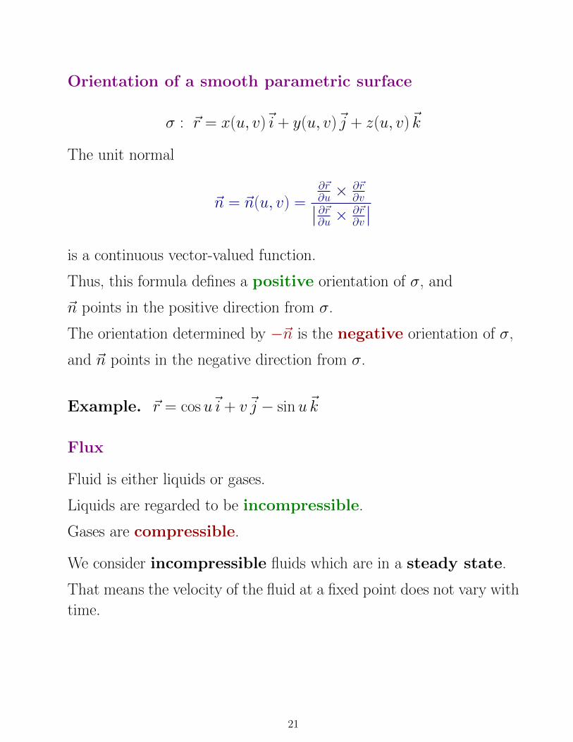
Orientation of a smooth parametric surface
σ : ~r = x(u, v)~i + y(u, v)~j + z(u, v)~k
The unit normal
~n = ~n(u, v) =∂~r∂u ×
∂~r∂v∣∣∂~r
∂u ×∂~r∂v
∣∣is a continuous vector-valued function.
Thus, this formula defines a positive orientation of σ, and
~n points in the positive direction from σ.
The orientation determined by −~n is the negative orientation of σ,
and ~n points in the negative direction from σ.
Example. ~r = cosu~i + v~j − sinu~k
Flux
Fluid is either liquids or gases.
Liquids are regarded to be incompressible.
Gases are compressible.
We consider incompressible fluids which are in a steady state.
That means the velocity of the fluid at a fixed point does not vary with
time.
21
Problem. An oriented surface σ is immersed in an incompressible,
steady-state fluid flow, and σ is permeable so that the fluid flows
through it freely. Find the net volume of the fluid Φ that passes through
σ per unit of time.
Net volume is the volume that passes through σ in the positive direc-
tion minus the volume that passes through σ in the negative direction.
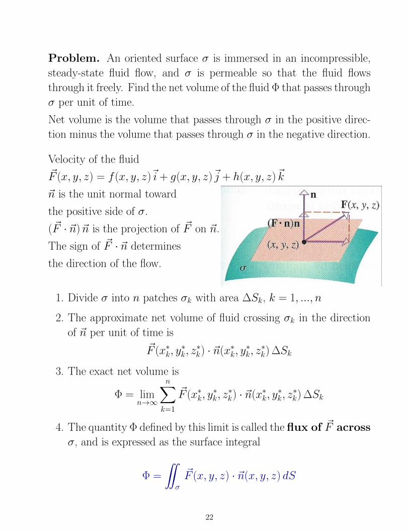
Velocity of the fluid
~F (x, y, z) = f (x, y, z)~i + g(x, y, z)~j + h(x, y, z)~k
~n is the unit normal toward
the positive side of σ.
(~F · ~n)~n is the projection of ~F on ~n.
The sign of ~F · ~n determines
the direction of the flow.
1. Divide σ into n patches σk with area ∆Sk, k = 1, ..., n
2. The approximate net volume of fluid crossing σk in the direction
of ~n per unit of time is
~F (x∗k, y∗k, z∗k) · ~n(x∗k, y
∗k, z∗k) ∆Sk
3. The exact net volume is
Φ = limn→∞
n∑k=1
~F (x∗k, y∗k, z∗k) · ~n(x∗k, y
∗k, z∗k) ∆Sk
4. The quantity Φ defined by this limit is called the flux of ~F across
σ, and is expressed as the surface integral
Φ =
¨σ
~F (x, y, z) · ~n(x, y, z) dS
22

Evaluating flux integrals
The integrals of the form˜σ~F · ~n dS are called flux integrals.
To calculate them we use
¨σ
~F · ~n dS =
¨R
~F · ~n∣∣∣∣∂~r∂u × ∂~r
∂v
∣∣∣∣ dA =
¨R
~F ·∂~r∂u ×
∂~r∂v∣∣∂~r
∂u ×∂~r∂v
∣∣∣∣∣∣∂~r∂u × ∂~r
∂v
∣∣∣∣ dA=
¨R
~F ·(∂~r
∂u× ∂~r
∂v
)dA
Example. ~F = z ~k, σ : x2 + y2 + z2 = a2 oriented outward.
Φ =?. Answer : 4π3 a
3
Let σ : z = g(x, y), ~r = u~i + v~j + g(u, v)~k
This choice of u, v imposes positive and negative orientations on σ.
Write σ as G(x, y, z) = z − g(x, y). Then
~n =~∇G∣∣∣~∇G∣∣∣ , ~∇G =
∂~r
∂u× ∂~r
∂v
because ~∇G is ⊥ σ, and ~∇G = ~k + · · · and ∂~r∂u ×
∂~r∂v = ~k + · · ·
Thus,
¨σ
~F · ~n dS =
¨R
~F · ~∇GdA =
¨R
~F ·(−∂z∂x~i− ∂z
∂y~j + ~k
)dA
if σ is oriented up (along the positive z-axis).
23
Example. z = 1− x2 − y2 and z ≥ 0. ~F = ~r. Φ =?.
Answer : 3π/2.
Similarly, let
σ : y = g(z, x) , ~r = v~i + g(u, v)~j + u~k , G(x, y, z) = y − g(z, x)
It is oriented along the positive y-axis.
or let
σ : x = g(y, z) , ~r = g(u, v)~i + u~j + v ~k , G(x, y, z) = x− g(y, z)
It is oriented along the positive x-axis.
Then
~n =~∇G∣∣∣~∇G∣∣∣ , ~∇G =
∂~r
∂u× ∂~r
∂v
and
¨σ
~F · ~n dS =
¨R
~F · ~∇GdA
24

6 The Divergence Theorem
Consider surfaces that are boundaries of finite solids – the surface of a
solid sphere, a solid box, a solid cylinder.
Such surfaces are said to be closed.
A piecewise smooth surface consists of finitely many smooth sur-
faces joined together at the edges (e.g. a box or a solid cylinder).
We consider only piecewise smooth
surfaces that can be assigned an
inward orientation (towards the interior
of the solid) and an outward orientation
(away from the interior).
The divergence of ~F = f (x, y, z)~i + g(x, y, z)~j + h(x, y, z)~k is
div ~F =∂f
∂x+∂g
∂y+∂h
∂z
The Divergence or Gauss’s Theorem. Let G be a solid whose
surface σ is oriented outward, and let ~n be the outward unit normal
on σ, then
¨σ
~F · ~n dS =
˚G
div ~F dV
where~F = f (x, y, z)~i + g(x, y, z)~j + h(x, y, z)~k
and f , g, h have continuous first partial derivatives on some open set
containing G.
25

The flux of a vector field across a closed surface with outward orien-
tation is equal to the triple integral of the divergence over the region
enclosed by the surface.
For G being simultaneously a simple
xy-, yz- and zx-solid the formula splits
¨σ
f~i · ~n dS =
˚G
∂f
∂xdV
¨σ
g~j · ~n dS =
˚G
∂g
∂ydV
¨σ
h~k · ~n dS =
˚G
∂h
∂zdV
We have for a simple xy-solid
˚G
∂h
∂zdV =
¨R
[ˆ g2(x,y)
g1(x,y)
∂h
∂z
]dz dA
=
¨R
[h(x, y, g2(x, y))− h(x, y, g1(x, y))] dA
¨σ
h~k · ~n dS =
¨σ1
h~k · ~n dS +
¨σ2
h~k · ~n dS
=
¨R
h(x, y, g1(x, y))~k · (∂z∂x~i +
∂z
∂y~j − ~k) dA
+
¨R
h(x, y, g2(x, y))~k · (−∂z∂x~i− ∂z
∂y~j + ~k) dA
where we have taken into account that
~k · ~n∣∣σ3
= 0 ⇒¨
σ3
h~k · ~n dS = 0
26

Example. Find the flux of the vector field
F(x, y, z) = (−3x+12xy2+4z3) i−(2y2−y+4x2) j+(4+3z+5yz−4y3) k
across the surface σ: x2 + y2 + z2 = 9 with outward orientation.
Answer : flux = 40685 π
Divergence viewed as flux density
Let G be small, e.g. a ball of radius ε << 1 centred at P0.
Φ(G) =
¨σ(G)
~F ·~n dS =
˚G
div ~F dV ≈ div ~F (P0)
˚G
dV = div ~F (P0)V
Thus
div ~F (P0) ≈ Φ(G)
vol(G)
where Φ(G)vol(G) is called the outward flux density of ~F across G.
Taking the limit vol(G)→ 0 (ε→ 0), we get
div ~F (P0) = limvol(G)→0
Φ(G)
vol(G)= lim
vol(G)→0
1
vol(G)
¨σ(G)
~F · ~n dS .
This limit is called the outward flux density of ~F at P0.
It tells us that in a steady-state fluid flow, div ~F can be interpreted as
the limiting flux per unit volume at a point.
27
Sources and sinks
Consider an incompressible fluid which means that its density is con-
stant. Consider a point P0 in fluid, and a small sphere G centred at
P0. If div ~F (P0) > 0 then Φ(G) > 0, and more fluid goes out through
the sphere than comes in. Since the fluid is incompressible this can
only happen if fluid is entering the flow at P0 otherwise the density
would decrees. Similarly, if div ~F (P0) < 0 then Φ(G) < 0, then fluid
is leaving the flow at P0. In an incompressible fluid, points at which
div ~F (P0) > 0 are called sources, and points at which div ~F (P0) < 0
are called sinks. If there are no sources and sinks we have
div ~F (P ) = 0 for every point P
This is the continuity equation for incompressible fluids.
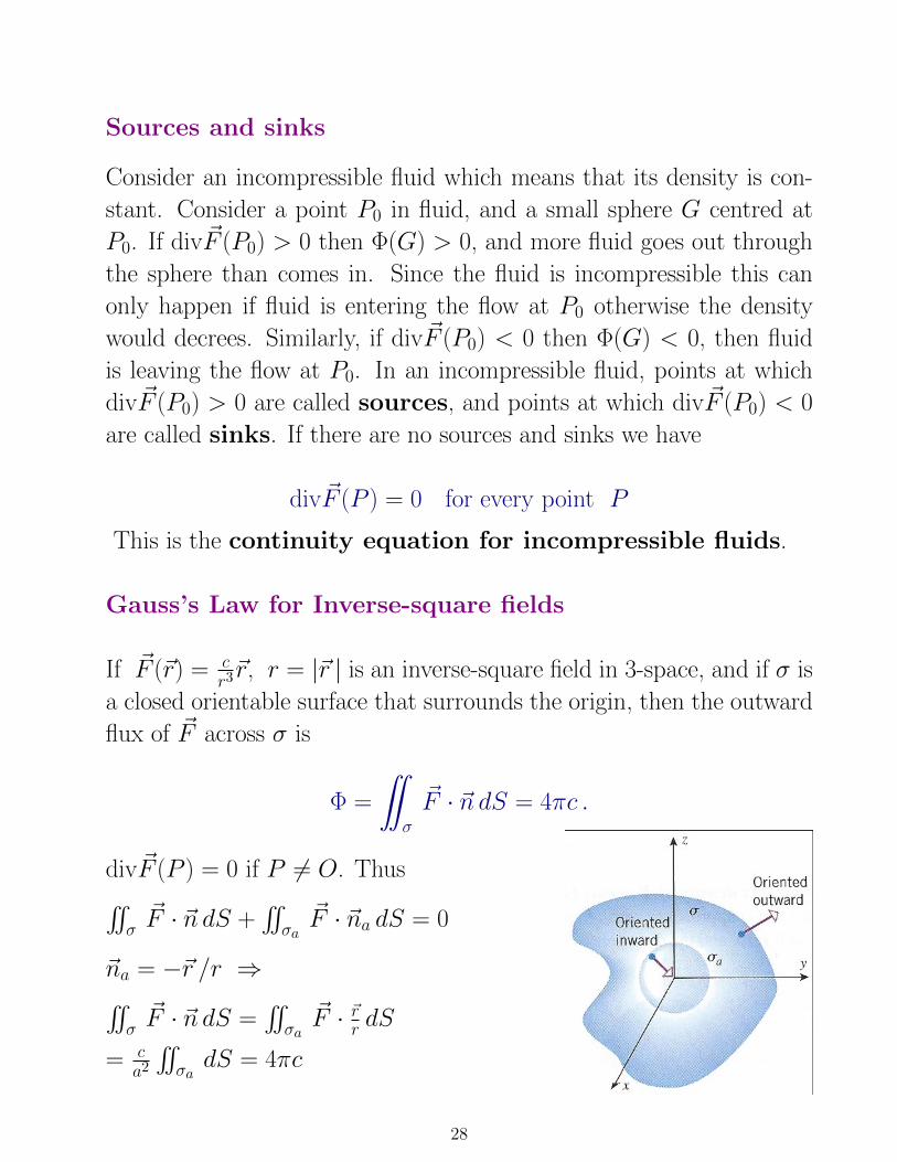
Gauss’s Law for Inverse-square fields
If ~F (~r) = cr3~r, r = |~r | is an inverse-square field in 3-space, and if σ is
a closed orientable surface that surrounds the origin, then the outward
flux of ~F across σ is
Φ =
¨σ
~F · ~n dS = 4πc .
div ~F (P ) = 0 if P 6= O. Thus˜σ~F · ~n dS +
˜σa~F · ~na dS = 0
~na = −~r /r ⇒˜σ~F · ~n dS =
˜σa~F · ~rr dS
= ca2
˜σadS = 4πc
28

7 Stoke’s Theorem
Let σ be a piecewise smooth oriented surface that is bounded by a
simple, closed, piecewise smooth curve C with positive orientation. If
the components of ~F (x, y, z) = f (x, y, z)~i+ g(x, y, z)~j + h(x, y, z)~k
are continuous and have continuous first partial derivatives on some
open set containing σ, then
˛C
~F · d~r =
˛C
~F · ~T ds =
¨σ
(curl~F ) · ~n dS
where ~T is the unit tangent vector to C, and
curl~F =
(∂h
∂y− ∂g
∂z
)~i−(∂h
∂x− ∂f
∂z
)~j+
(∂g
∂x− ∂f
∂y
)~k =
∣∣∣∣∣∣∣~i ~j ~k∂∂x
∂∂y
∂∂z
f g h
∣∣∣∣∣∣∣ = ~∇×~F
Example. Let C be the triangle in the plane z = 14y with ver-
tices (0, 0, 0), (2, 0, 0) and (0, 4, 1) with a counterclockwise orientation
looking down the positive z-axis. Use Stokes’ Theorem to evaluate¸C F · dr.
F(x, y, z) = (2xy + 3x + 4z) i− (2x2 − 5y) j + (y − z) k
Answer : −20
29

Green’s theorem as a particular case of Stoke’s theorem
Let’s regard~F (x, y) = f (x, y)~i + g(x, y)~j
as a vector filed in 3-space
~F (x, y, z) = f (x, y)~i + g(x, y)~j + 0~k
Let σ = R where R is a region in the xy-plane. Then
‰C
~F · d~r =
¨R
(curl~F ) · ~k dA
Since
curl~F =
(∂g
∂x− ∂f
∂y
)~k
we get Green’s theorem
‰C
f dx + g dy =
¨R
(∂g
∂x− ∂f
∂y
)dA
30