Variants of Kalman Filter for the Synchronization of

11

Variants of Kalman Filter for the Synchronization of Chaotic Systems

Sadasivan Puthusserypady1 and Ajeesh P. Kurian2 1Department of Electrical and Computer Engineering, National University of Singapore

2Department of Electrical and Computer Engineering, University of Calgary 1Singapore

2Canada

1. Introduction

Perhaps the most important lesson to be drawn from the study of nonlinear dynamical

systems over the past few decades is that even simple dynamical systems can give rise to

complex behaviour which is statistically indistinguishable from that produced by a complex

random process. Chaotic systems are nonlinear systems which exhibit such complex

behaviour. In such systems, the state variables move in a bounded, aperiodic, random-like

fashion. A distinct property of chaotic dynamics is its long-term unpredictability. In such

systems, initial states which are very close to each other produce markedly different

trajectories. When nearby points evolve to result in uncorrelated trajectories, while forming

the same attractor, the dynamical system is said to possess sensitive dependence to initial

conditions (Devaney, 1985). Due to these desirable properties, application of chaotic systems

are explored for many engineering applications such as secure communications, data

encryption, digital water marking, pseudo random number generation etc (Kennedy et. al.,

2000). In most of these applications, it is essential to synchronize the chaotic systems at two

different locations. In this chapter, we explore the Kalman filter based chaotic

synchronization.

2. Synchronization of chaotic systems

Related works of synchronization dates back to the research carried out by Fujisaka and Yamada in 1983 (Fujisaka & Yamada, 1983). Pecora and Carroll suggested a drive-response system for synchronization of chaotic systems. They showed that if all the transversal Lyapunov exponents of the response system are negative, the systems synchronize asymptotically (Pecora & Carrol, 1990). Later a plethora of research work was reported on synchronization of chaotic systems (Nijmeijer & Mareels, 1997). One of the well researched approaches is the coupled synchronization, where a proper coupling is introduced between the transmitter and the receiver. The chaotic systems synchronize asymptotically when the coupling strength is above a certain threshold, which is determined by the local Lyapunov exponents (Suchichik et. al., 1997). Let the transmitter and the receiver states of the chaotic systems be given by

Source: Kalman Filter, Book edited by: Vedran Kordić, ISBN 978-953-307-094-0, pp. 390, May 2010, INTECH, Croatia, downloaded from SCIYO.COM

www.intechopen.com

Kalman Filter

210

1 ( , )k k μ+ =x f x (1.a)

1ˆ ˆ ˆ( , )k k

μ+ =x f x (1.b)

where 1 , ,Tn

k k kx x⎡ ⎤= …⎣ ⎦x and 1ˆ ˆ ˆ, ,Tn

k k kx x⎡ ⎤= …⎣ ⎦x are the n-dimensional state vectors of the

transmitter and the receiver systems, respectively. μ and μ are the transmitter and the

receiver system parameters and 1[ (.), , (.)]n Tf f= …f is a smooth nonlinear vector valued

function. Normally, we have a noisy observation at the receiver which is given by

( )k k k= +y h x v (2)

where kv is the channel noise and (.)h is the measurement function. These two systems are

said to be synchronized if

ˆlim 0.k kk→∞ − =x x (3)

2.1 Coupled synchronization

In coupled synchronization, a coupling is introduced between the transmitter and the receiver as:

−= + −1ˆ ˆ ˆ( ) ( )k k k k kx f x K y y (4)

where kK is the appropriate coupling coefficient matrix. In conventional coupled

synchronization, kK is set to be a constant value such that the global and local Lyapunov

exponents (The Lyapunov exponents of a dynamic system are the quantities that

characterize the rate of divergence/convergence of the trajectories generated by

infinitesimally close initial conditions under the dynamics ) are negative. This makes the

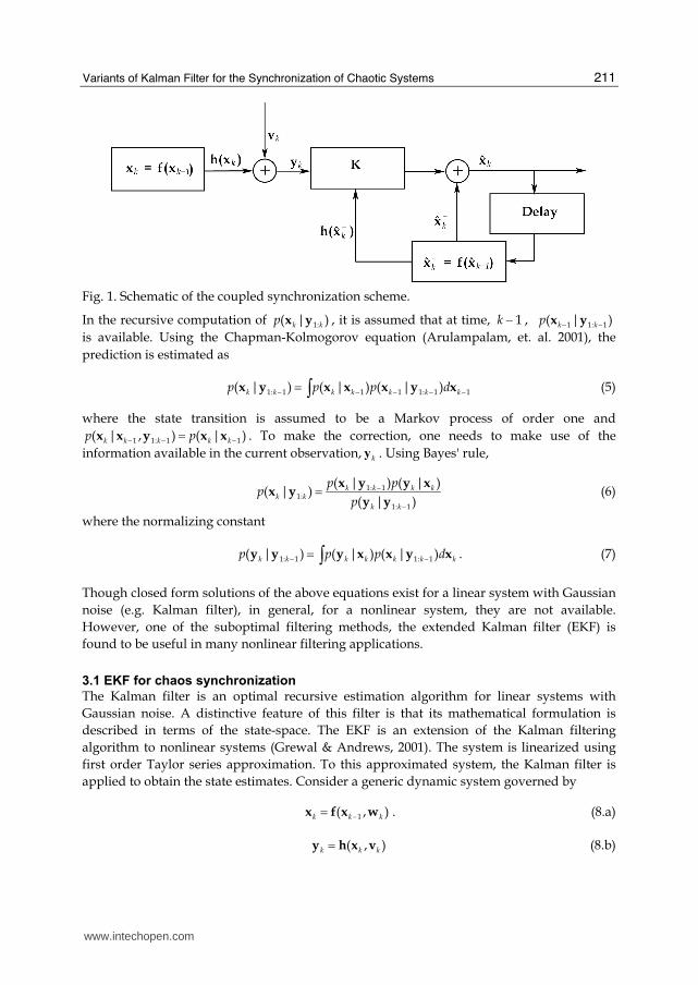
receiver to synchronize with the transmitter asymptotically. The schematic of the coupled

synchronization is shown in Fig. 1. This method of synchronization can be treated as a

predictor corrector filter approach. In general, a predictive filter predicts the subsequent

states and corrects it with additional information available from the observation. Due to the

measurement and the channel noises in a communication system, stochastic techniques

have to be applied for synchronization. Instead of keeping kK as a constant value if it is

determined adaptively, the coupled synchronization has a similarity with the predictive

filtering techniques.

3. Chaos synchronization: a stochastic estimation view point

In stochastic state estimation methods, one would like to estimate the state variable kx based

on the set of all available (noisy) measurement 1: 1{ , , }k k= …y y y with certain degree of

confidence. This is done by constructing the conditional probability density function (pdf),

1:( | )k kp x y (i.e. the probability of kx given the observations, 1:ky ), known as the posterior

probability. It is assumed that 0 0( | )p x y is available. In predictor corrector filtering

methods, 1:( | )k kp x y is obtained recursively by a prediction step which is estimated without

the knowledge of current measurement, ky followed by a correction step where the

knowledge of ky is used to make the correction to the predicted values.

www.intechopen.com


211

Fig. 1. Schematic of the coupled synchronization scheme.

In the recursive computation of 1:( | )k kp x y , it is assumed that at time, 1k − , 1 1: 1( | )k kp − −x y

is available. Using the Chapman-Kolmogorov equation (Arulampalam, et. al. 2001), the

prediction is estimated as

1: 1 1 1 1: 1 1( | ) ( | ) ( | )k k k k k k kp p p d− − − − −= ∫x y x x x y x (5)

where the state transition is assumed to be a Markov process of order one and

1 1: 1 1( | , ) ( | )k k k k kp p− − −=x x y x x . To make the correction, one needs to make use of the

information available in the current observation,ky . Using Bayes' rule,

1: 11:

1: 1

( | ) ( | )( | )

( | )k k k k

k k

k k

p pp

p−

−= x y y x

x yy y

(6)

where the normalizing constant

1: 1 1: 1( | ) ( | ) ( | )k k k k k k kp p p d− −= ∫y y y x x y x . (7)

Though closed form solutions of the above equations exist for a linear system with Gaussian

noise (e.g. Kalman filter), in general, for a nonlinear system, they are not available.

However, one of the suboptimal filtering methods, the extended Kalman filter (EKF) is

found to be useful in many nonlinear filtering applications.

3.1 EKF for chaos synchronization

The Kalman filter is an optimal recursive estimation algorithm for linear systems with

Gaussian noise. A distinctive feature of this filter is that its mathematical formulation is

described in terms of the state-space. The EKF is an extension of the Kalman filtering

algorithm to nonlinear systems (Grewal & Andrews, 2001). The system is linearized using

first order Taylor series approximation. To this approximated system, the Kalman filter is

applied to obtain the state estimates. Consider a generic dynamic system governed by

1( , )k k k−=x f x w . (8.a)

( , )k k k=y h x v (8.b)

www.intechopen.com

Kalman Filter

212

where the process noise, kw , and observation (measurement) noise, kv , are zero mean

Gaussian processes with covariance matrices kQ and kR , respectively. In minimum mean

square estimation (MMSE), the receiver computes ˆkx which is an estimate of kx from the

available observations 1: 1{ , , }k k= …y y y such that the mean square error (MSE), Tk k

⎡ ⎤⎣ ⎦e eE

(where ˆk k k= −e x x ), is minimized. The EKF algorithm for the state estimation is given by,

| 1 1ˆ ˆ( ,0),k k k− −=x f x (9.a)

| 1 1 1 1T T

k k k k k k k k− − − −= +P F P F W Q W (9.b)

In the above equations, the notation | 1k k − denotes an operation performed at time

instant, k , using the information available till 1k − . At time instant k , | 1ˆ

k k−x is the a priori

estimate of the state vector kx , | 1k k−P is the a priori error covariance matrix, 1k−F is the

Jacobian of (.)f with respect to the state vector 1k−x and kW is the Jacobian of (.)f with

respect to the noise vector k

w . The EKF update equations are:

{ } 1

| 1 | 1T T T

k k k k k k k k k k k

−− −= +K P H H P H VR V (10.a)

| 1ˆ ˆ ˆ( )k k k k k k−= + −x x K y y (10.b)

| 1( )k k k k k−= −P I K H P (10.c)

where kK is the Kalman gain, kH is the Jacobian of (.)h with respect to | 1ˆ

k k−x , ˆkx is the a

posteriori estimate of the state vector, kV is the Jacobian of (.)h with respect to the noise

vector kv , and kP is the a posterior error covariance matrix. When EKF is used for

synchronization of chaotic maps, kK acts as the coupling strength which is updated

iteratively. Schematic of EKF based synchronization is shown in Fig. 2.

K kDelay

f (x k− 1 , 0)

x k |k− 1

x k

h(x k |k− 1 , 0)

yk

yk

+

−

Fig. 2. Schematic of EKF based chaos synchronization

3.2.1 Convergence analysis

Convergence analysis of kK can be carried out by studying the convergence of | 1k k−P . At any

time instant, k , according to the matrix fraction propagation of | 1k k−P , it can be shown that

(Grewal & Andrews, 2001),

1| 1k k k k

−− =P A B , (11)

www.intechopen.com


213

where kA and 1k−B are factors of | 1k k−P . If kF is nonsingular (i.e. the map is invertible), then

1k+A and 1k+B are given by the recursive equation as

1

1

11

T T Tk kk k k k k k k k

T T Tk kk k k k k

− − −+− − −+

⎡ ⎤+⎡ ⎤ ⎡ ⎤= ⎢ ⎥⎢ ⎥ ⎢ ⎥⎣ ⎦ ⎣ ⎦⎣ ⎦A AF W F H R H W F

B BF H R H F. (12)

From the above expression, it can be shown that, when there is no process noise (i.e.

k =W 0 and kF is contractive (i.e. the magnitudes of its eigenvalues are less than one),

| 1k k−P will converge in time. However, inside the chaotic attractor, the behaviour of | 1k k−P is

aperiodic if kF is time varying. This behaviour has dramatic influence on the convergence of

Kalman filter based synchronization system (Kurian, 2006) for systems with hyperbolic

tangencies (HTs).

3.3 Unscented Kalman filter

The approximation error introduced by the EKF together with the expansions of this error at the HTs makes the system unstable and diverging trajectories are generated at the receiver. One way to mitigate this problem is to use nonlinear filters with better approximation capabilities. Unscented Kalman filter (UKF) has shown to possess these capabilities (Julier & Uhlman, 2004). It is essentially an approximation method to solve Eq. (5). UKF works based on the principle of unscented transform (UT) (Julier & Uhlman, 1997).

Fig. 3. Illustration of unscented transform (UT).

In Fig. 3, the UT of a random variable, u , which undergoes a nonlinear transformation

( ( )f u ) to result in another random variable, v is shown. To calculate the statistics of v , the

ideal solution is to get posterior density, ( )p v , analytically from the prior density ( )p u . The

mean and covariance of v can also be computed analytically. However, this is highly

impractical in most of the situations because of the nonlinearity. UT is a method for

www.intechopen.com

Kalman Filter

214

approximating the statistics of a random variable which undergoes a nonlinear

transformation. It uses carefully selected vectors ( iU ), known as sigma points, to

approximate the statistics of the posterior density. Each sigma point is associated with a

weight iW . The number of sigma points is 2 1n + where n is the dimension of the state

vector. With the knowledge of the mean ( u ) and covariance ( uP ) of the prior density, these

sigma points are constructed as

( )( ) ( )( ) ( )

κκ

κ κκ κ

⎛ ⎞= =⎜ ⎟+⎝ ⎠⎛ ⎞= + + = …⎜ ⎟+⎝ ⎠⎛ ⎞= − + = + …⎜ ⎟+⎝ ⎠

0 0ˆ, , ; 0

1ˆ, ( ) , ; 1, ,

2( )

1ˆ, ( ) , ; 1, ,2

2( )

i ii

i ii

W in

W n i nn

W n i n nn

u

u

u

u P

u P

U

U

U

(13)

where κ is a scaling parameter and ( )( )i

n κ+ uP is the ith row or column of the square

root of the matrix, ( )n κ+ uP . These sigma points are propagated through the nonlinearity

(.)f to obtain

( ) for 0,1, ,2 .i i i n= = …fV U (14)

Using the set of iV , the mean ( v ) and covariance ( vP ) of the posterior density is estimated as

=

=∑20

ˆn

i ii

Wv V (15.a)

( )( )=

= − −∑20

ˆ ˆ .n

T

i i ii

WvP v vV V (15.b)

It is shown that the UKF based approximation is equivalent to a third order Taylor series

approximation if the Gaussian prior is assumed (Julier & Uhlman, 2004). Another advantage

of UT is that it does not require the calculation of the Jacobian or Hessian.

3.3.1 Scaled unscented transform

The scaled unscented transform (SUT) is a generalization of the UT. It is a method that

scales an arbitrary set of sigma points yet capture the mean and covariance correctly. The

new transform is given by

( )0 0' for 0, ,2i i i nα= + − = …U U U U (16)

where α is a positive scaling parameter. By this the distribution of the sigma points can be

controlled without affecting the positive definitive nature of the matrix, ( )n κ+ uP . A set of

sigma points, [ ] [ ]{ }0 2 0 2, , , , ,n nW W= … = …U WU U , is first calculated using Eq.(13) and then

transformed into scaled sigma points, { }' ' '2

' '0 2

'0, , , , ,n nW W⎡ ⎤ ⎡ ⎤= … = …⎣ ⎦ ⎣ ⎦U WU U by

www.intechopen.com


215

( )'0 0 for 0,1, ,2i i i nα= + − = …U U U U (17.a)

02 2

2

'

1(1 ) 0

0i

i

Wi

WW

i

α αα

⎧ + − =⎪⎪= ⎨⎪ ≠⎪⎩. (17.b)

The sigma point selection and scaling can be combined to a single step by setting

2( )n nλ α κ= + − (18)

and

='0 uU (19.a)

( )0 ˆ ( ) 1, ,i

i

n i nλ= + + = …u

u PU (19.b)

( )λ= − + = + …' ˆ ( ) 1, ,2ii

n i n nuu PU (19.c)

( )0

mWn

λλ= + (19.d)

( ) 20 (1 )

( )cW

n

λ α βλ= + − ++ (19.e)

( ) ( ) 1for 1,2, ,2 .

2( )m c

i iW W i nnλ= = = …+ (19.f)

Parameter β above is another control parameter which affects the weighting of the zeroth

sigma point for the calculation of the covariance. Using SUT, the mean and the covariance

can be estimated as

=

=∑2 ( ) '

0

ˆn

mi i

i

Wv V (20.a)

( )( )=

= − −∑2 ( ) ' '

0

ˆ ˆTc

ii

i

n

iWvP v vV V (20.b)

where ( )i i′ ′= fV U .

Selection of κ is such that it should result in positive semi definiteness of the covariance

matrix. 0κ ≥ guarantees this condition and a good choice is 0κ = . Choose 0 1α≤ ≤ and

0β ≥ . For Gaussian prior density, 2β = is an optimal choice. Since, α controls the spread

of the sigma points, it is selected such that it should not capture the non-local effects when

nonlinearities are strong.

www.intechopen.com

Kalman Filter

216

3.3.2 Unscented Kalman filter

UKF is an application of the SUT. It implements the minimum mean square estimates as

follows. The objective is to estimate the stateskx , given the observations, 1:ky . For this, the

state variable is redefined as the concatenation of the original state and noise variables (i.e. T

a T T T

k k k k⎡ ⎤= ⎣ ⎦x x w v with dimension

an ). The steps involved in UKF are listed below. First, we

initialize the parameters

=0 0ˆ [ ]x xE (21.a)

( )( )⎡ ⎤= − −⎣ ⎦0 0 0 0 0ˆ ˆ T

P x x x xE (21.b)

⎡ ⎤= ⎣ ⎦0 0ˆ ˆ

Ta Tx x 0 0 (21.c)

0

0a

⎡ ⎤⎢ ⎥= ⎢ ⎥⎢ ⎥⎣ ⎦

P 0 0

P 0 Q 0

0 0 R

(21.d)

For 1,2,k = … calculate the sigma points:

λ− − − −⎡ ⎤= ± +⎣ ⎦1 1 1 1ˆ ˆ ( )a a a a

k k k a knx x PX (22)

Time update:

( )| 1 1 1,x wk k k k− − −= fX X X (23.a)

− −==∑2 ( )

| 1 , | 10

ân

m xk k i i k k

i

Wx X (23.b)

− − − − −=⎡ ⎤ ⎡ ⎤= − −⎣ ⎦ ⎣ ⎦∑2 ( )

| 1 , | 1 | 1 , | 1 | 10

ˆ ân

Tc x xk k i i k k k k i k k k k

i

WP x xX X (23.c)

( )| 1 | 1 | 1,x vk k k k k k− − −= hY X X (23.d)

− −==∑2 ( )

| 1 , | 10

ân

mk k i i k k

i

Wy Y (23.e)

Measurement update:

− − − −=⎡ ⎤ ⎡ ⎤= − −⎣ ⎦ ⎣ ⎦∑2 ( )

ˆ ˆ , | 1 | 1 , | 1 | 10

ˆ â

k k

nTc

i i k k k k i k k k ki

Wy yP y yY Y (24.a)

− − − −=⎡ ⎤ ⎡ ⎤= − −⎣ ⎦ ⎣ ⎦∑2 ( )

ˆ ˆ , | 1 | 1 , | 1 | 10

ˆ â

k k

nTc

i i k k k k i k k k ki

Wx yP x xX Y (24.b)

www.intechopen.com


217

−= 1ˆ ˆ ˆ ˆk k k kk x y y yK P P (24.c)

" " "( )| 1 | 1k k k k k k k− −= + −x x K y y (24.d)

−= − ˆ ˆ| 1 k k

Tk k k k ky yP P K P K (24.e)

It is shown in (Julier & Uhlman, 2004) that the approximation introduced by the UKF has more number of Taylor series terms. The effect of the approximation errors is different for different nonlinear systems. In some cases, if the nonlinearity is quadratic, approximation error will not have any strong influence.

4. Results and discussion

To assess the performance of the EKF and UKF based synchronization schemes, simulation studies are carried out on three different chaotic systems/maps1: (i) Ikeda map (IM), (ii) Lorenz system, and (iii) Mackey-Glass (MG) system. The Lorenz system is a three

dimensional vector field, 3 3( , , ) :x y z R Rφ → , representing the interrelation of temperature

variation and convective motion. The set of coupled differential equations representing the Lorenz system is given by

( ) ( ( ) ( ))x t y t x tσ= −$ (25.a)

= − + −$( ) ( ) ( ) ( ) ( )y t x t z t rx t y t (25.b)

( ) ( ) ( ) ( )z t x t y t cz t= −$ (25.c)

where 10σ = , 28r = and 8 / 3c = are used to obtain the Lorenz attractor. The three states

( ,x y and z ) are randomly initialized and the system of differential equation is solved with

the fourth order Runge-Kutta method. The Lorenz attractor is shown in Fig. 4. Ikeda map represent a discrete dynamic system of pumped laser beam around a lossy ring cavity and is defined as

ωφ+

⎡ ⎤⎛ ⎞⎢ ⎥⎜ ⎟= + − −⎜ ⎟⎢ ⎥+⎝ ⎠⎣ ⎦1 2exp 1

1k k

k

z p Bzz

(26)

where kz is a complex-valued state variable with 1R I

k k kz x x= + − . Here, R

kx is { }

kzℜ and I

kx

is { }kzℑ . {.}ℜ and {.}ℑ give the real and imaginary parts of a complex variable, respectively.

For the set of parameters = 0.92p , = 0.9B ,φ = 0.4 , and ω = 6 , the attractor of this map is

shown in Fig. 5. The Mackey-Glass system was originally proposed as a first order nonlinear delay differential equation to describe physiological control systems. It is given by

1 Map is used to represent discrete dynamic systems. i.e. →:f X X

www.intechopen.com

Kalman Filter

218

-40-20

020

40 -40-20

020

4060

10

20

30

40

50

60

70

80

y(t)

x(t)

z(t

)

Fig. 4. Lorenz attractor.

ττ

−= − + + −$10

( )( ) ( )

1 ( )

bx tx t ax t

x t (27)

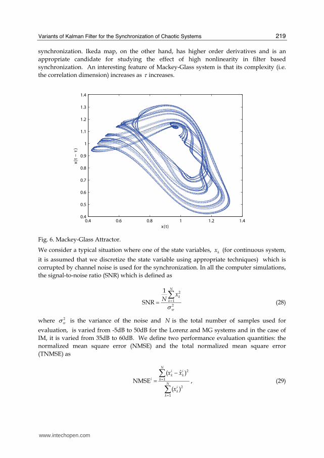
This system is chaotic for values of = 0.1a and τ ≥ 17 . Figure 6 shows the Mackey-Glass

attractor with τ =17.

-0.4 -0.2 0 0.2 0.4 0.6 0.8 1 1.2 1.4 1.6

-1.5

-1

-0.5

0

0.5

ℜ{zk}

ℑ{zk}

Fig. 5. Ikeda map attractor.

These systems/maps have distinct dynamical properties and well suited for our analysis.

Lorenz system is one of the archetypical chaotic systems commonly studied for chaotic

www.intechopen.com


219

synchronization. Ikeda map, on the other hand, has higher order derivatives and is an

appropriate candidate for studying the effect of high nonlinearity in filter based

synchronization. An interesting feature of Mackey-Glass system is that its complexity (i.e.

the correlation dimension) increases as τ increases.

0.4 0.6 0.8 1 1.2 1.40.4

0.5

0.6

0.7

0.8

0.9

1

1.1

1.2

1.3

1.4

x(t)

x(t−τ)

Fig. 6. Mackey-Glass Attractor.

We consider a typical situation where one of the state variables, kx (for continuous system,

it is assumed that we discretize the state variable using appropriate techniques) which is

corrupted by channel noise is used for the synchronization. In all the computer simulations,

the signal-to-noise ratio (SNR) which is defined as

σ== ∑ 2

12

1

SNR

N

kk

w

xN

(28)

where 2wσ is the variance of the noise and N is the total number of samples used for

evaluation, is varied from -5dB to 50dB for the Lorenz and MG systems and in the case of

IM, it is varied from 35dB to 60dB. We define two performance evaluation quantities: the

normalized mean square error (NMSE) and the total normalized mean square error

(TNMSE) as

2

1

2

1

ˆ( )

NMSE

( )

Ni ik k

i kN

ik

k

x x

x

=

=

−=∑∑ , (29)

www.intechopen.com

Kalman Filter

220

1

TNMSE NMSEn

i

i==∑ , (30)

respectively. While NMSE gives an idea about the recovery of observed state variable,

TNMSE gives how faithfully, the attractor can be reconstructed.

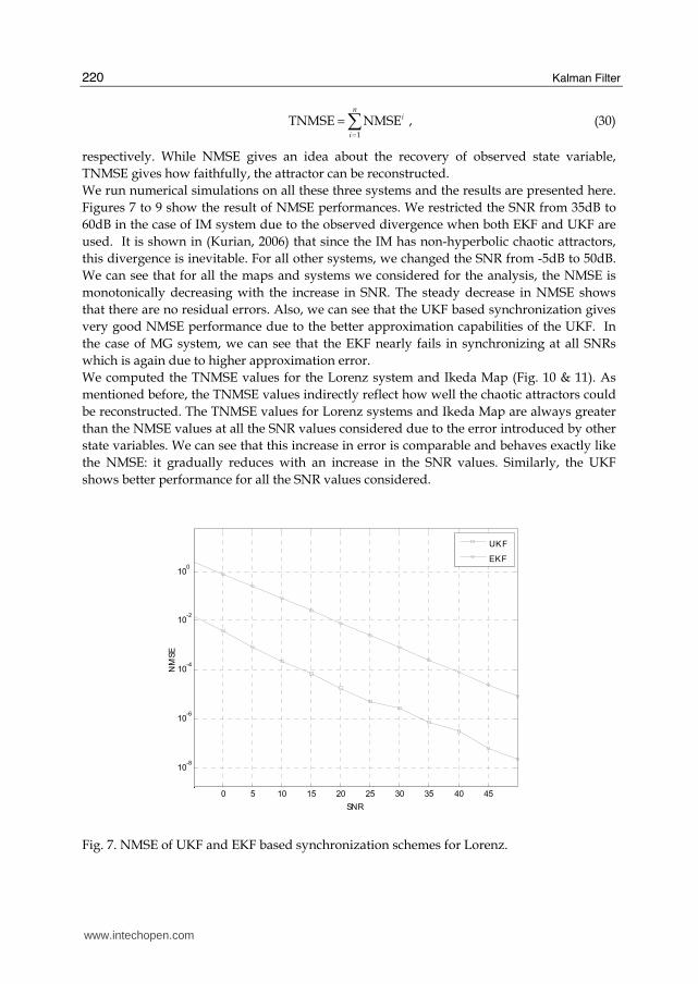
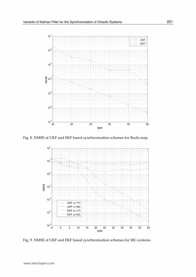
We run numerical simulations on all these three systems and the results are presented here.

Figures 7 to 9 show the result of NMSE performances. We restricted the SNR from 35dB to

60dB in the case of IM system due to the observed divergence when both EKF and UKF are

used. It is shown in (Kurian, 2006) that since the IM has non-hyperbolic chaotic attractors,

this divergence is inevitable. For all other systems, we changed the SNR from -5dB to 50dB.

We can see that for all the maps and systems we considered for the analysis, the NMSE is

monotonically decreasing with the increase in SNR. The steady decrease in NMSE shows

that there are no residual errors. Also, we can see that the UKF based synchronization gives

very good NMSE performance due to the better approximation capabilities of the UKF. In

the case of MG system, we can see that the EKF nearly fails in synchronizing at all SNRs

which is again due to higher approximation error.

We computed the TNMSE values for the Lorenz system and Ikeda Map (Fig. 10 & 11). As

mentioned before, the TNMSE values indirectly reflect how well the chaotic attractors could

be reconstructed. The TNMSE values for Lorenz systems and Ikeda Map are always greater

than the NMSE values at all the SNR values considered due to the error introduced by other

state variables. We can see that this increase in error is comparable and behaves exactly like

the NMSE: it gradually reduces with an increase in the SNR values. Similarly, the UKF

shows better performance for all the SNR values considered.

0 5 10 15 20 25 30 35 40 45

10-8

10-6

10-4

10-2

100

SNR

NM

SE

UKF

EKF

Fig. 7. NMSE of UKF and EKF based synchronization schemes for Lorenz.

www.intechopen.com


221

35 40 45 50 55 6010

-7

10-6

10-5

10-4

10-3

10-2

10-1

SNR

NM

SE

UKF

EKF

Fig. 8. NMSE of UKF and EKF based synchronization schemes for Ikeda map.

-5 0 5 10 15 20 25 30 35 40 45 5010

-6

10-5

10-4

10-3

10-2

10-1

100

SNR

NM

SE

UKF (τ=17)

UKF (τ=50)

EKF (τ=17)

EKF (τ=50)

Fig. 9. NMSE of UKF and EKF based synchronization schemes for MG systems.

www.intechopen.com

Kalman Filter

222

-5 0 5 10 15 20 25 30 35 40 45 5010

-8

10-6

10-4

10-2

100

102

SNR

NM

SE

UKF

EKF

Fig. 10. TNMSE of UKF and EKF based synchronization schemes for Lorenz system.

35 40 45 50 55 6010

-6

10-5

10-4

10-3

10-2

10-1

SNR

TN

MSE

UKF

EKF

Fig. 11. TNMSE of UKF and EKF based synchronization schemes for Ikeda map.

www.intechopen.com


223

5. Conclusions

Chaotic systems are simple dynamic systems which can display very complex behavior. One of the defining characteristics of such systems is the sensitive dependence on initial conditions and hence synchronization of such systems possesses certain amount of difficulties. This task will be even more formidable when the channels as well as the measurement noises are present in the system. Stochastic methods are applied to synchronize such chaotic systems. EKF is one of the most widely investigated stochastic filtering methods for chaotic synchronization. However, for highly nonlinear systems, EKF introduces approximation errors causing unacceptable degradation in the system performance. We consider UKF, which has better approximation error characteristics for chaos synchronization and show that it has better error characteristics.

6. References

R. L. Devaney (1985). An introduction to chaotic dynamical system. The Benjamin Cummings

Publishing Company Inc.

M. P. Kennedy, R. Rovatti, and G. Setti (2000). Chaotic electronics in telecommunications. CRC

Press.

Fujisaka, H. & Yamada (1983). Stability theory of synchronized motion in coupled oscillator

systems. Progressive Theory of Physics. Vol. 69, No. 1, pp. 32–47.

Pecora, L. M. & Carroll, T. L. (1990). Synchronization in chaotic systems. Physical Review

Letters. Vol. 64, pp. 821–824.

Ogorzalek, M. J. (1993). Taming chaos–Part I: Synchronization. IEEE Trans. Circuits Syst.–I.

vol. 40, No. 10, pp. 693–699.

Sushchik, M. M.; Rulkov, N. F. & Abarbanel H. D. I. (1997). Robustness and stability of

synchronized chaos: An illustrative model. IEEE Trans. Circuits Syst.–I, vol. 44, pp.

867–873.

Nijmeijer, H. & Mareels, I. M. Y. (1997). An observer looks at synchronization. IEEE Trans.

Circuits Sys.–I, vol. 44, No. 10, pp. 882–890.

Arulampalam, S.; Maskell, S. ; Gordon, N. & Clapp, T. (2001). A tutorial on particle filters for

on–line non–linear/non–Gaussian Bayesian tracking. IEEE Trans. Signal Process.,

vol. 50, pp. 174–188.

Grewal, M. S. & Andrews A. P. (2001). Kalman filtering: Theory and practice using MATLAB,

2nd Ed., John Wiley & Sons.

Kurian, A. (2006). Performance analysis of filtering based chaotic synchronization and development

of chaotic digital communication schemes. PhD Dissertation, National University of

Singapore.

Julier, S. J. & Uhlman, J. K. (2004). Unscented Kalman filtering and nonlinear estimation.

Proc. IEEE, vol. 92, pp. 401–421.

Eric, A. W. & van der Merwe, R. (2000). The unscented Kalman filter for nonlinear

estimation, Proc. IEEE Symposium on Adaptive Systems for Signal Processing,

Communication and Control (AS-SPCC). Lake Louise, Alberta, Canada, Octobre.

www.intechopen.com

Kalman Filter

224

Julier, S. J. & Uhlmann, J. K. (1997). A new extension of the Kalman filter to nonlinear

systems. Proc. of AeroSense: The 11th International Symposium on Aerospace/Defense

Sensing, Simulation and Control.

H. D. I. Abarbanel, Analysis of observed chaotic data. Springer, USA, 1996.

www.intechopen.com

Kalman FilterEdited by Vedran Kordic

ISBN 978-953-307-094-0Hard cover, 390 pagesPublisher InTechPublished online 01, May, 2010Published in print edition May, 2010

InTech EuropeUniversity Campus STeP Ri Slavka Krautzeka 83/A 51000 Rijeka, Croatia Phone: +385 (51) 770 447 Fax: +385 (51) 686 166www.intechopen.com

InTech ChinaUnit 405, Office Block, Hotel Equatorial Shanghai No.65, Yan An Road (West), Shanghai, 200040, China

Phone: +86-21-62489820 Fax: +86-21-62489821

The Kalman filter has been successfully employed in diverse areas of study over the last 50 years and thechapters in this book review its recent applications. The editors hope the selected works will be useful toreaders, contributing to future developments and improvements of this filtering technique. The aim of this bookis to provide an overview of recent developments in Kalman filter theory and their applications in engineeringand science. The book is divided into 20 chapters corresponding to recent advances in the filed.

How to referenceIn order to correctly reference this scholarly work, feel free to copy and paste the following:

Sadasivan Puthusserypady and Ajeesh P. Kurian (2010). Variants of Kalman Filter for the Synchronization ofChaotic Systems, Kalman Filter, Vedran Kordic (Ed.), ISBN: 978-953-307-094-0, InTech, Available from:http://www.intechopen.com/books/kalman-filter/variants-of-kalman-filter-for-the-synchronization-of-chaotic-systems

© 2010 The Author(s). Licensee IntechOpen. This chapter is distributedunder the terms of the Creative Commons Attribution-NonCommercial-ShareAlike-3.0 License, which permits use, distribution and reproduction fornon-commercial purposes, provided the original is properly cited andderivative works building on this content are distributed under the samelicense.

https://creativecommons.org/licenses/by-nc-sa/3.0/

Documents

Variants of Kalman Filter for the Synchronization of