Kalman and Extended Kalman Filters:Concept, Derivation and Properties

Maria Isabel RibeiroInstitute for Systems and Robotics

Instituto Superior TecnicoAv. Rovisco Pais, 1

1049-001 Lisboa PORTUGAL{mir@isr.ist.utl.pt}

c©M. Isabel Ribeiro, 2004

February 2004

Contents

1 Introduction 2

2 The Filtering Problem 3

3 Estimation of Random Parameters. General Results 83.1 Problem Formulation . . . . . . . . . . . . . . . . . . . . . . . . 83.2 Problem Reformulation . . . . . . . . . . . . . . . . . . . . . . . 103.3 Particularization for Gaussian Random Vectors . . . . . . . . . . 12

4 The Kalman Filter 144.1 Kalman Filter dynamics . . . . . . . . . . . . . . . . . . . . . . . 154.2 One-step ahead prediction dynamics . . . . . . . . . . . . . . . . 224.3 Kalman filter dynamics for a linear time-invariant system . . . . . 234.4 Steady-state Kalman filter . . . . . . . . . . . . . . . . . . . . . . 244.5 Initial conditions . . . . . . . . . . . . . . . . . . . . . . . . . . 254.6 Innovation Process . . . . . . . . . . . . . . . . . . . . . . . . . 274.7 The Kalman filter dynamics and the error ellipsoids . . . . . . . . 29

5 The Extended Kalman Filter 315.1 Derivation of Extended Kalman Filter dynamics . . . . . . . . . . 34

1

Chapter 1

Introduction

This report presents and derives the Kalman filter and the Extended Kalman filterdynamics. The general filtering problem is formulated and it is shown that, un-der linearity and Gaussian conditions on the systems dynamics, the general filterparticularizes to the Kalman filter. It is shown that the Kalman filter is a linear,discrete time, finite dimensional time-varying system that evaluates the state esti-mate that minimizes the mean-square error.

The Kalman filter dynamics results from the consecutive cycles of predictionand filtering. The dynamics of these cycles is derived and interpreted in the frame-work of Gaussian probability density functions. Under additional conditions onthe system dynamics, the Kalman filter dynamics converges to a steady-state fil-ter and the steady-state gain is derived. The innovation process associated withthe filter, that represents the novel information conveyed to the state estimate bythe last system measurement, is introduced. The filter dynamics is interpreted interms of the error ellipsoids associated with the Gaussian pdf involved in the filterdynamics.

When either the system state dynamics or the observation dynamics is non-linear, the conditional probability density functions that provide the minimummean-square estimate are no longer Gaussian. The optimal non-linear filter prop-agates these non-Gaussian functions and evaluate their mean, which represents anhigh computational burden. A non optimal approach to solve the problem, in theframe of linear filters, is the Extended Kalman filter (EKF). The EKF implementsa Kalman filter for a system dynamics that results from the linearization of theoriginal non-linear filter dynamics around the previous state estimates.

2

Chapter 2

The Filtering Problem

This section formulates the general filtering problem and explains the conditionsunder which the general filter simplifies to a Kalman filter (KF).

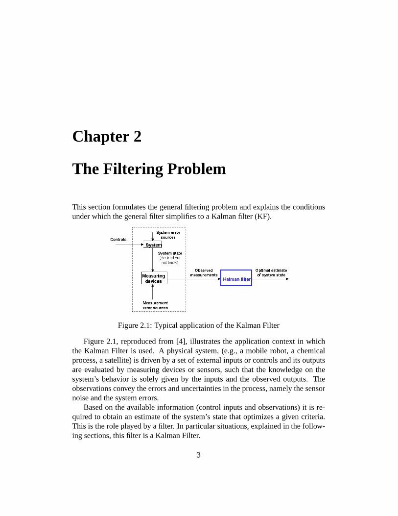
Figure 2.1: Typical application of the Kalman Filter

Figure 2.1, reproduced from [4], illustrates the application context in whichthe Kalman Filter is used. A physical system, (e.g., a mobile robot, a chemicalprocess, a satellite) is driven by a set of external inputs or controls and its outputsare evaluated by measuring devices or sensors, such that the knowledge on thesystem’s behavior is solely given by the inputs and the observed outputs. Theobservations convey the errors and uncertainties in the process, namely the sensornoise and the system errors.

Based on the available information (control inputs and observations) it is re-quired to obtain an estimate of the system’s state that optimizes a given criteria.This is the role played by a filter. In particular situations, explained in the follow-ing sections, this filter is a Kalman Filter.

3

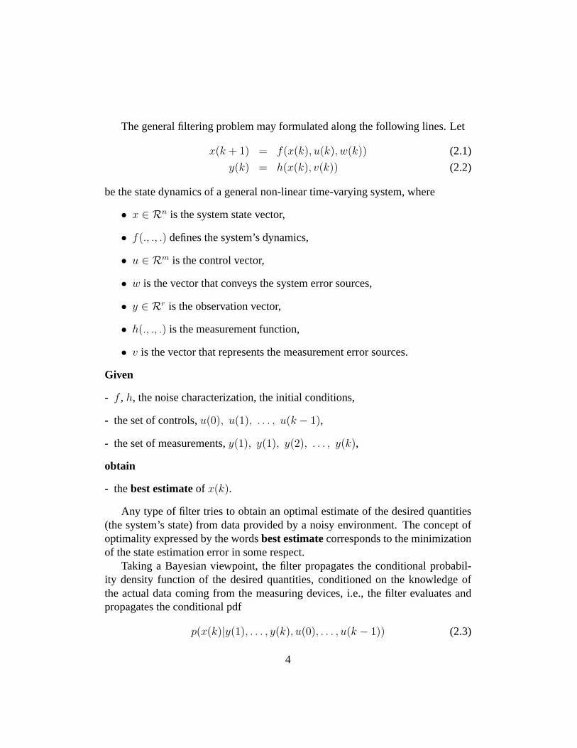
The general filtering problem may formulated along the following lines. Let

x(k + 1) = f(x(k), u(k), w(k)) (2.1)

y(k) = h(x(k), v(k)) (2.2)

be the state dynamics of a general non-linear time-varying system, where

• x ∈ Rn is the system state vector,

• f(., ., .) defines the system’s dynamics,

• u ∈ Rm is the control vector,

• w is the vector that conveys the system error sources,

• y ∈ Rr is the observation vector,

• h(., ., .) is the measurement function,

• v is the vector that represents the measurement error sources.

Given

- f , h, the noise characterization, the initial conditions,

- the set of controls,u(0), u(1), . . . , u(k − 1),

- the set of measurements,y(1), y(1), y(2), . . . , y(k),

obtain

- thebest estimateof x(k).

Any type of filter tries to obtain an optimal estimate of the desired quantities(the system’s state) from data provided by a noisy environment. The concept ofoptimality expressed by the wordsbest estimatecorresponds to the minimizationof the state estimation error in some respect.

Taking a Bayesian viewpoint, the filter propagates the conditional probabil-ity density function of the desired quantities, conditioned on the knowledge ofthe actual data coming from the measuring devices, i.e., the filter evaluates andpropagates the conditional pdf

p(x(k)|y(1), . . . , y(k), u(0), . . . , u(k − 1)) (2.3)

4

for increasing values ofk. This pdf conveys the amount of certainty on the knowl-edge of the value ofx(k).

Consider that, for a given time instantk, the sequence of past inputs and thesequence of past measurements are denoted by1

Uk−10 = {u0, u1, . . . , uk−1} (2.4)

Y k1 = {y1, y2, . . . , yk}. (2.5)

The entire system evolution and filtering process, may be stated in the follow-ing steps, [1], that considers the systems dynamics (2.1)-(2.2):

• Given x0

- Nature applyw0,

- We applyu0,

- The system moves to statex1,

- We make a measurementy1.

• Question: which is the best estimate ofx1?Answer: is obtained fromp(x1|Y 1

1 , U00 )

- Nature applyw1,

- We applyu1,

- The system moves to statex2,

- We make a measurementy2.

• Question: which is the best estimate ofx2?Answer: is obtained fromp(x2|Y 2

1 , U10 )

- ...

- ...

- ...

- ...

• Question: which is the best estimate ofxk−1?Answer: is obtained fromp(xk−1|Y k−1

1 , Uk−20 )

- Nature applywk−1,

- We applyuk−1,

- The system moves to statexk,

1Along this textu(i) = ui, y(i) = yi andx(i) = xi.

5

- We make a measurementyk.

• Question: which is the best estimate ofxk?Answer: is obtained fromp(xk|Y k

1 , Uk−10 )

- ...

- ...

- ...

- ...

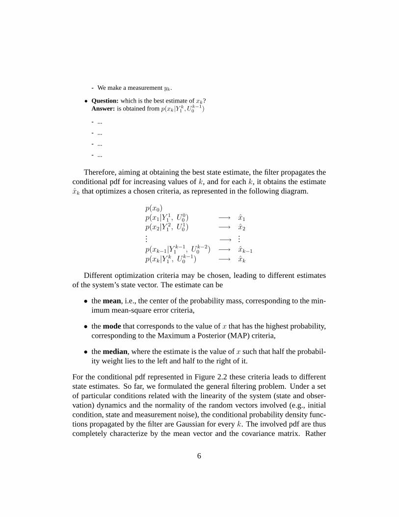
Therefore, aiming at obtaining the best state estimate, the filter propagates theconditional pdf for increasing values ofk, and for eachk, it obtains the estimatexk that optimizes a chosen criteria, as represented in the following diagram.

p(x0)p(x1|Y 1

1 , U00 ) −→ x1

p(x2|Y 21 , U1

0 ) −→ x2... −→ ...p(xk−1|Y k−1

1 , Uk−20 ) −→ xk−1

p(xk|Y k1 , Uk−1

0 ) −→ xk

Different optimization criteria may be chosen, leading to different estimatesof the system’s state vector. The estimate can be

• themean, i.e., the center of the probability mass, corresponding to the min-imum mean-square error criteria,

• themodethat corresponds to the value ofx that has the highest probability,corresponding to the Maximum a Posterior (MAP) criteria,

• themedian, where the estimate is the value ofx such that half the probabil-ity weight lies to the left and half to the right of it.

For the conditional pdf represented in Figure 2.2 these criteria leads to differentstate estimates. So far, we formulated the general filtering problem. Under a setof particular conditions related with the linearity of the system (state and obser-vation) dynamics and the normality of the random vectors involved (e.g., initialcondition, state and measurement noise), the conditional probability density func-tions propagated by the filter are Gaussian for everyk. The involved pdf are thuscompletely characterize by the mean vector and the covariance matrix. Rather

6

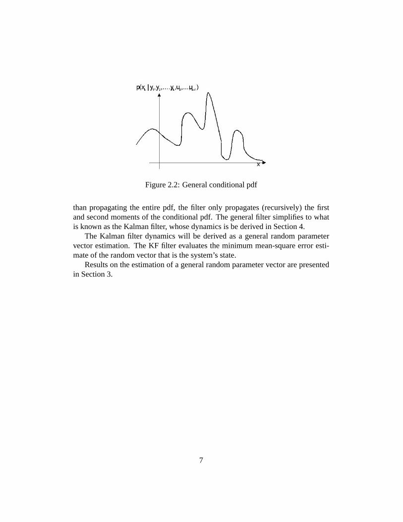
Figure 2.2: General conditional pdf

than propagating the entire pdf, the filter only propagates (recursively) the firstand second moments of the conditional pdf. The general filter simplifies to whatis known as the Kalman filter, whose dynamics is be derived in Section 4.

The Kalman filter dynamics will be derived as a general random parametervector estimation. The KF filter evaluates the minimum mean-square error esti-mate of the random vector that is the system’s state.

Results on the estimation of a general random parameter vector are presentedin Section 3.

7

Chapter 3

Estimation of Random Parameters.General Results

This section presents basic results on the estimation of a random parameter vectorbased on a set of observations. This is the framework in which the Kalman filterwill be derived, given that the state vector of a given dynamic system is interpretedas a random vector whose estimation is required. Deeper presentations of theissues of parameter estimation may be found, for example, in [3], [5], [10].

Letθ ∈ Rn (3.1)

be a random vector, from which the available information is given by a finite setof observations

Y k1 = [y(1), y(2), . . . , y(k − 1), y(k)] (3.2)

with no assumption on the dependency betweeny(i) andθ.Denote by

p(θ, Y k1 ), p(θ|Y k

1 ) e p(Y k1 )

the joint probability density function (pdf) ofθ andY k1 , the conditional pdf ofθ

givenY k1 , and the pdf ofY k

1 , respectively.

3.1 Problem Formulation

The estimation problem of the random vectorθ is stated, in general terms, asfollows: given the observationsy(1), y(2), ..., y(k), evaluate an estimate ofθ, i.e.,

θ(k) = f [y(i), i = 1, ..., k] (3.3)

8

that optimizes a given criteria. Common optimization criteria are:

• the mean square error,

• the maximum a posterior.

In the sequel we will consider the mean-square error estimator, and therefore,the estimated value of the random vector is such that the cost function

J [θ(k)] = E[θ(k)T θ(k)] (3.4)

is minimized, whereθ(k) stands for the estimation error given by

θ(k)4= θ − θ(k). (3.5)

According to the above formulated problem, the estimateθ(k) is given by

θ(k) = argminE[(θ − θ(k))T (θ − θ(k)]. (3.6)

We now show that minimizingE[θ(k)T θ(k)] relative toθ(k) is equivalent tominimize the condition meanE[θ(k)T θ(k)|Y k

1 ] relative toθ(k). In fact, from thedefinition of the mean operator, we have

E[θ(k)T θ(k)] =

∫ ∞

−∞

∫ ∞

−∞θ(k)T θ(k)p(θ, Y k

1 )dθdY k1 (3.7)

wheredθ = dθ1dθ2...dθn anddY k1 = dy1dy2...dyk. Using the result obtained from

Bayes law, (see e.g., [8])

p(θ, Y k1 ) = p(θ|Y k

1 )p(Y k1 ) (3.8)

in (3.7) yields:

E[θ(k)T θ(k)] =

∫ ∞

−∞

[∫ ∞

−∞θ(k)T θ(k)p(θ|Y k

1 )dθ

]p(Y k

1 )dY k1 .

Moreover, reasoning about the meaning of the integral inside the square brackets,results

E[θ(k)T θ(k)] =

∫ ∞

−∞E[θ(k)T θ(k)|Y k

1 ]p(Y k1 )dY k

1 .

Therefore, minimizing the mean value of the left hand side of the previous equalityrelative toθ(k) is equivalent to minimize, relative to the same vector, the meanvalueE[θ(k)T θ(k)|Y k

1 ] on the integral on the right hand side. Consequently, theestimation of the random parameter vector can be formulated in a different way,as stated in the following subsection.

9

3.2 Problem Reformulation

Given the set of observationsy(1), y(2), ..., y(k), the addressed problem is thederivation of an estimator ofθ that minimizes the conditional mean-square error,i.e.,

θ(k) = argminE[θ(k)T θ(k)|Y k1 ]. (3.9)

Result 3.2.1 : The estimator that minimizes the conditional mean-square error isthe conditional mean, [5], [10],

θ(k) = E[θ|Y k1 ]. (3.10)

Proof: From the definition of the estimation error in (3.5), the cost function in(3.9) can be rewritten as

J = E[(θ − θ(k))T (θ − θ(k))|Y k1 ] (3.11)

or else,

J = E[θT θ − θT θ(k)− θ(k)T θ + θ(k)T θ(k)|Y k1 ] (3.12)

= E[θT θ|Y k1 ]− E[θT |Y k

1 ]θ(k)− θ(k)T E[θ|Y k1 ] + E[θ(k)T θ(k)|Y k

1 ]. (3.13)

The last equality results from the fact that, by definition (see (3.3)),θ(k) is afunction ofY k

1 and thusE[θ(k)|Y k

1 ] = θ(k).

If we add and subtractE[θT |Y k1 ]E[θ|Y k

1 ] to (3.13) yields

J = E[θT θ|Y k1 ]− E[θT |Y k

1 ]E[θ|Y k1 ] + [θ(k)− E[θ|Y k

1 ]]T [θ(k)− E[θ|Y k1 ]]

where the first two terms in the right hand side do not depend onθ(k). The de-pendency ofθ(k) onJ results from a quadratic term, and therefore it is immediatethatJ achieves a minimum when the quadratic term is zero, and thus

θ(k) = E[θ|Y k1 ],

which concludes the proof.2

Corollary 3.2.1 : Consider thatf(Y k1 ) is a given function of the observations

Y k1 . Then, the estimation error is orthogonal tof(Y k

1 ), θ − θ(k) ⊥ f(Y k1 ), this

meaning thatE[(θ − θ(k))fT (Y k

1 )] = 0. (3.14)

10

Proof: For the proof we use the following result on jointly distributed randomvariables. Letx andy be jointly distributed random variables andg(y) a functionof y. It is known that, [8]

E[xg(y)] = E [E(x|y)g(y)] (3.15)

where the outer mean-value operator in the right hand side is defined relative tothe random variabley. Using (3.15) in the left hand side of (3.14) results

E[θ(k)fT (Y k1 )] = E[E(θ(k)|Y k

1 )fT (Y k1 )]. (3.16)

Evaluating the mean value of the variable inside the square brackets in (3.16)leads to

E[θ(k)|Y k1 ] = E[θ|Y k

1 ]− θ(k) (3.17)

becauseθ(k) is known whenY k1 is given. Therefore, (3.17) is zero, from where

(3.14) holds, this concluding the proof.2

The particularization of the corollary for the case wheref(Y k1 ) = θ(k) yields,

E[θ(k)θT (k)] = 0. (3.18)

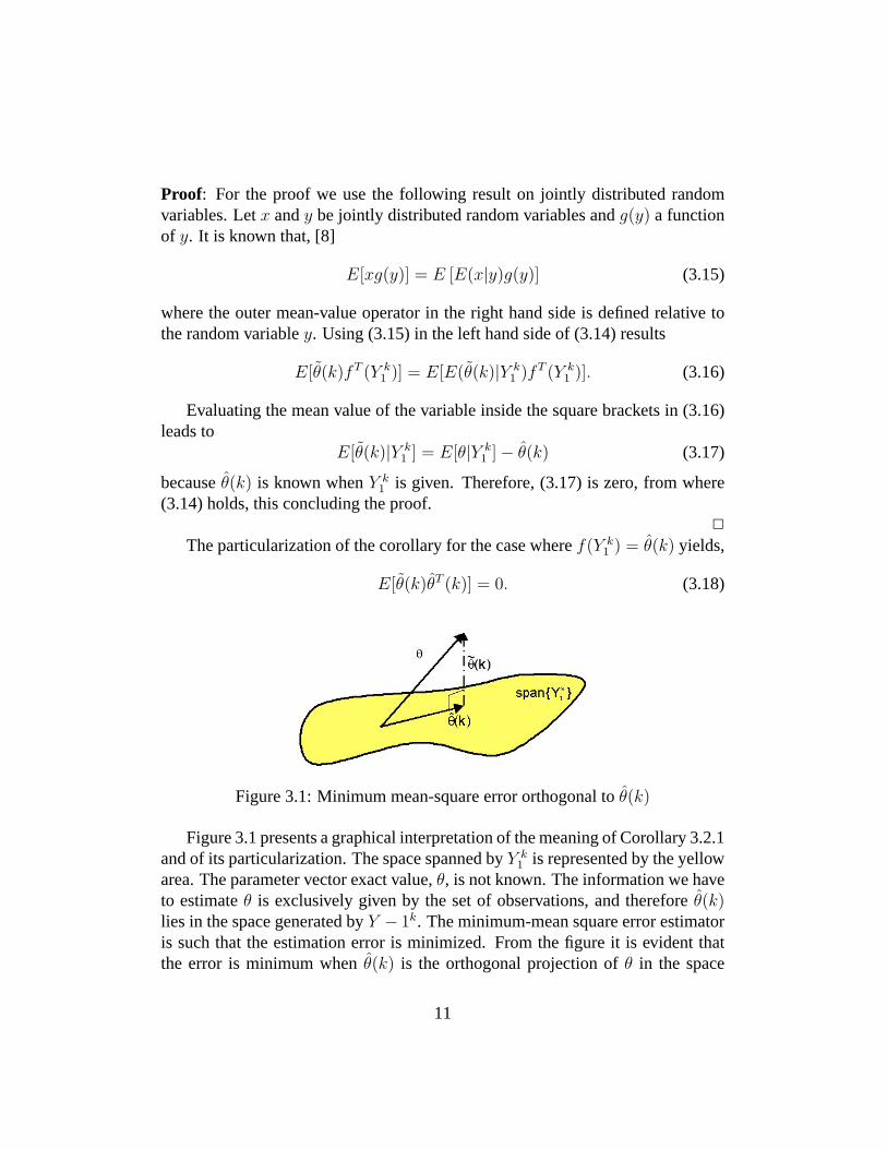
Figure 3.1: Minimum mean-square error orthogonal toθ(k)

Figure 3.1 presents a graphical interpretation of the meaning of Corollary 3.2.1and of its particularization. The space spanned byY k

1 is represented by the yellowarea. The parameter vector exact value,θ, is not known. The information we haveto estimateθ is exclusively given by the set of observations, and thereforeθ(k)lies in the space generated byY − 1k. The minimum-mean square error estimatoris such that the estimation error is minimized. From the figure it is evident thatthe error is minimum whenθ(k) is the orthogonal projection ofθ in the space

11

spanned byY k1 . Therefore, the estimation errorθ(k) is orthogonal to the space of

the observations, as expressed in (3.18).The results derived so far, made no assumptions on the type of the probability

density functions involved. In the next subsection the previous results are partic-ularized for the Gaussian case.

3.3 Particularization for Gaussian Random Vectors

The Result 3.2.1 is valid for any joint distribution ofθ andY k1 , i.e., it does not

particularize the joint pdf of these variables.It is well known from the research community dealing with estimation and

filtering theory that many results simplify when assuming that the involved vari-ables are Gaussian. This subsection discusses the simplifications resulting fromconsidering thatθ andY k

1 in Result 3.2.1 are jointly Gaussian.

Result 3.3.1 If θ eY k1 are jointly Gaussian random vectors, then,

E[θ|Y k1 ] = E[θ] + RθY k

1R−1

Y k1[Y k

1 − E[Y k1 ]], (3.19)

where

RθY k1

= E[(θ − E(θ))(Y k1 − E(Y k

1 )T ], (3.20)

RY k1 Y k

1= E[(Y k

1 − E(Y k1 ))(Y k

1 − E(Y k1 )T ]. (3.21)

The previous result is very important. It states that, whenθ e Y k1 are jointly

Gaussian, the estimatior ofθ that minimizes the conditional mean-square error is alinear combination of the observations. In fact, note that (3.19) may be rewrittenas

E[θ|Y k1 ] = f(E(θ), E(Y k

1 )) +k∑

i=1

WiYi, (3.22)

making evident the linear combination of the observations involved.Whenθ andY k

1 , are not jointly Gaussian then, in general terms,E[θ|Y k1 ] is a

non linear function of the observations.

Result 3.3.2 In the situation considered in Result 3.3.1,θ(k) is an unbiased esti-mate ofθ, i.e.,

E[θ(k)] = E[θ]. (3.23)

12

Result 3.3.3 In the situation considered in Result 3.3.1,θ(k) is a minimum vari-ance estimator.

Result 3.3.4 In the situation considered in Result 3.3.1,θ(k) and θ(k) are jointlydistributed Gaussian random vectors.

For the proofs of the three previous results see [5]. A result, related withResult 3.3.1, is now presented.

Result 3.3.5 Consider thatθ e Y k1 are not jointly Gaussian, butE[θ], E[Y k

1 ],RY k

1 Y k1

andRθY k1

are known. Then, thelinear estimator that minimizes the meansquare error is (still) given by

θ(k) = E[θ] + RθY k1R−1

Y k1

(Y k

1 − E[Y k1 ]

). (3.24)

Note that the minimization in Result 3.3.5 is subject to the constraint of havinga linear estimator while in Result 3.3.1 no constraint is considered. If the linearestimator constraint in Result 3.3.5 was not considered, the minimum mean squareerror estimator will generally yield an estimateθ(k) as anon-linear function ofthe observations.

13

Chapter 4

The Kalman Filter

Section 2 presented the filtering problem for a general nonlinear system dynamics.Consider now that the system represented in Figure 2.1 has a linear time-varyingdynamics, i.e., that (2.1)-(2.2) particularizes to,

xk+1 = Akxk + Bkuk + Gwk k ≥ 0 (4.1)

yk = Ckxk + vk (4.2)

wherex(k) ∈ Rn, u(k) ∈ Rm, w(k) ∈ Rn, v(k) ∈ Rr, y(k) ∈ Rr, {wk} and{vk} are sequences of white, zero mean, Gaussian noise with zero mean

E[wk] = E[vk] = 0, (4.3)

and joint covariance matrix

E

[(wk

vk

)(wT

k vTk )

]=

[Qk 00 Rk

]. (4.4)

The initial state,x0, is a Gaussian random vector with mean

E[x0] = x0 (4.5)

and covariance matrix

E[(x0 − x0)(x0 − x0)T ] = Σ0. (4.6)

The sequence{uk} is deterministic.

14

The problem of state estimation was formulated in Section 2. It can also beconsidered as the estimation of a random parameter vector, and therefore the re-sults in Section 3 hold.

For the system (4.1)-(4.2), the Kalman filter is the filter that obtains the min-imum mean-square state error estimate. In fact, whenx(0) is a Gaussian vector,the state and observations noisesw(k) andv(k) are white and Gaussian and thestate and observation dynamics are linear,

1. the conditional probability density functionsp(xk)|Y k1 , Uk−1

0 ) are Gaussianfor anyk,

2. the mean, the mode, and the median of this conditional pdf coincide,

3. the Kalman filter, i.e., the filter that propagates the conditional pdfp(xk)|Y k1 , Uk−1

0 )and obtains the state estimate by optimizing a given criteria, is the best filteramong all the possible filter types and it optimizes any criteria that might beconsidered.

Letp(xk)|Y k

1 , Uk−10 ) ∼ N (x(k|k), P (k|k)) (4.7)

represent the conditional pdf as a Gaussian pdf. The state estimatex(k|k) is theconditional mean of the pdf and the covariance matrixP (k|k) quantifies the un-certainty of the estimate,

x(k|k) = E[x(k)|Y k1 , Uk−1

0 ]

P (k|k) = E[(x(k)− x(k|k))(x(k)− x(k|k))T |Y k1 , Uk−1

0 ].

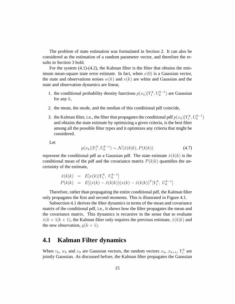
Therefore, rather than propagating the entire conditional pdf, the Kalman filteronly propagates the first and second moments. This is illustrated in Figure 4.1.

Subsection 4.1 derives the filter dynamics in terms of the mean and covariancematrix of the conditional pdf, i.e., it shows how the filter propagates the mean andthe covariance matrix. This dynamics is recursive in the sense that to evaluatex(k + 1|k + 1), the Kalman filter only requires the previous estimate,x(k|k) andthe new observation,y(k + 1).

4.1 Kalman Filter dynamics

Whenvk, wk andx0 are Gaussian vectors, the random vectorsxk, xk+1, Y k1 are

jointly Gaussian. As discussed before, the Kalman filter propagates the Gaussian

15

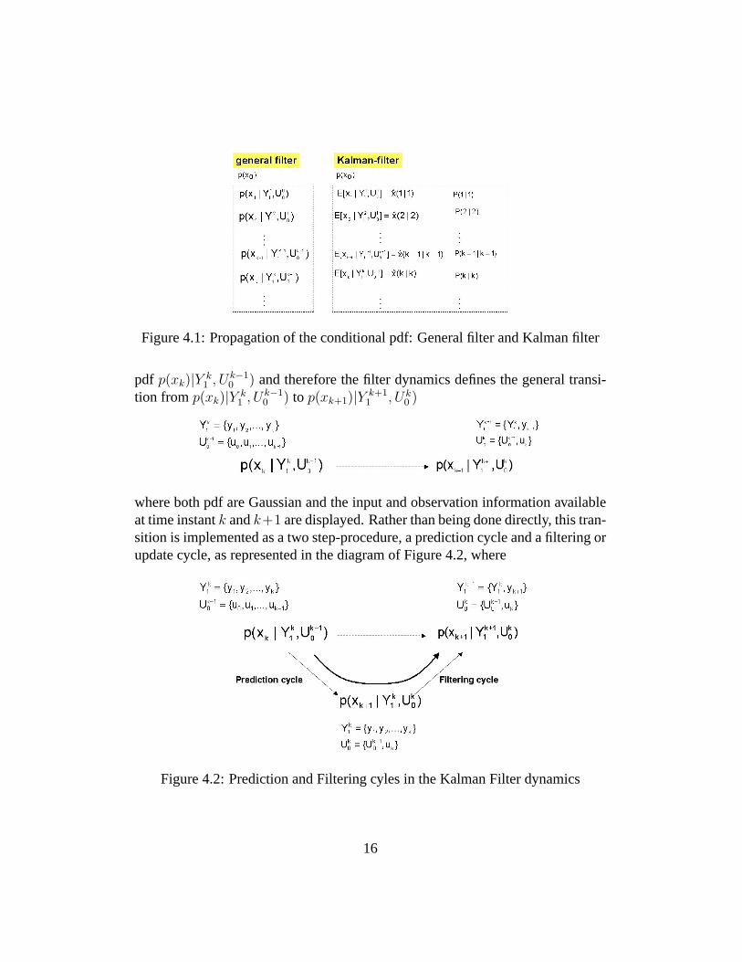
Figure 4.1: Propagation of the conditional pdf: General filter and Kalman filter

pdf p(xk)|Y k1 , Uk−1

0 ) and therefore the filter dynamics defines the general transi-tion fromp(xk)|Y k

1 , Uk−10 ) to p(xk+1)|Y k+1

1 , Uk0 )

where both pdf are Gaussian and the input and observation information availableat time instantk andk+1 are displayed. Rather than being done directly, this tran-sition is implemented as a two step-procedure, a prediction cycle and a filtering orupdate cycle, as represented in the diagram of Figure 4.2, where

Figure 4.2: Prediction and Filtering cyles in the Kalman Filter dynamics

16

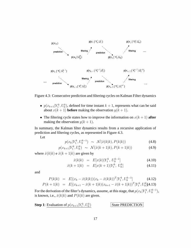
Figure 4.3: Consecutive prediction and filtering cycles on Kalman Filter dynamics

• p(xk+1|Y k1 , Uk

0 ), defined for time instantk + 1, represents what can be saidaboutx(k + 1) beforemaking the observationy(k + 1).

• The filtering cycle states how to improve the information onx(k + 1) aftermaking the observationy(k + 1).

In summary, the Kalman filter dynamics results from a recursive application ofprediction and filtering cycles, as represented in Figure 4.3.

Letp(xk|Y k

1 , Uk−10 ) ∼ N (x(k|k), P (k|k)) (4.8)

p(xk+1|Y k1 , Uk

0 ) ∼ N (x(k + 1|k), P (k + 1|k)) (4.9)

wherex(k|k) e x(k + 1|k) are given by

x(k|k) = E[x(k)|Y k1 , Uk−1

0 ] (4.10)

x(k + 1|k) = E[x(k + 1)|Y k1 , Uk

0 ] (4.11)

and

P (k|k) = E[(xk − x(k|k))(xk − x(k|k))T |Y k1 , Uk−1

0 ] (4.12)

P (k + 1|k) = E[(xk+1 − x(k + 1|k)(xk+1 − x(k + 1|k))T |Y k1 , Uk

0 ].(4.13)

For the derivation of the filter’s dynamics, assume, at this stage, thatp(xk|Y k1 , Uk−1

0 ),is known, i.e.,x(k|k) andP (k|k) are given.

Step 1: Evaluation ofp(xk+1|Y k1 , Uk

0 ) State PREDICTION

17

This Gaussian pdf is completely characterized by the mean and covariancematrix. Applying the mean value operator on both sides of (4.1), yields

E[xk+1|Y k1 , Uk

0 ] = AkE[xk|Y k1 , Uk

0 ]+BkE[uk|Y k1 , Uk

0 ]+GE[wk|Y k1 , Uk

0 ]. (4.14)

Taking (4.8) and (4.9) into account, considering thatwk e Y k1 are independent

random vectors and thatwk has zero mean, we obtain:

x(k + 1|k) = Akx(k|k) + Bkuk. (4.15)

Defining theprediction error as

x(k + 1|k)4= x(k + 1)− x(k + 1|k) (4.16)

and replacing in this expression the values ofx(k + 1) andx(k + 1|k) yields:

x(k + 1|k) = Akxk + Bkuk + Gkwk − Akx(k|k)−Bkuk = Akx(k|k) + Gkwk

(4.17)where thefiltering error was defined similarly to (4.16)

x(k|k)4= x(k)− x(k|k). (4.18)

Given thatx(k|k) andwk are independent, from (4.17) we have

E[x(k +1|k)x(k +1|k)T |Y k1 , Uk

0 ] = AkE[x(k|k)|Y k1 , Uk

0 ]ATk +GkQGT

k . (4.19)

Including in (4.19) the notations (4.12) and (4.13) results:

P (k + 1|k) = AkP (k|k)ATk + GkQkG

Tk . (4.20)

The predicted estimate of the system’s state and the associated covariance ma-trix in (4.15) and (4.20), correspond to the best knowledge of the system’s state attime instantk + 1 before making the observation at this time instant. Notice thatthe prediction dynamics in (4.15) follows exactly the system’s dynamics in (4.1),which is the expected result given that the system noise has zero mean.

Step 2: Evaluation ofp(yk+1|Y k1 , Uk

0 ) Measurement PREDICTION

From (4.2), it is clear that

p(yk+1|Y k1 , Uk

0 ) = p(Ck+1xk+1 + vk+1|Y k1 , Uk

0 ) (4.21)

18

and thus, as this is a Gaussian pdf, thepredicted measurementis given by

y(k + 1|k) = E[yk+1|Y k1 , Uk

0 ] = Ck+1xk+1|k. (4.22)

Defining the measurement prediction error as

y(k + 1|k)4= yk+1 − y(k + 1|k), (4.23)

and replacing the values ofy(k + 1) andy(k + 1|k) results:

y(k + 1|k) = Ck+1x(k + 1|k) + vk+1. (4.24)

Therefore, the covariance matrix associated to (4.24) is given by

Py(k + 1|k) = Ck+1P (k + 1|k)CTk+1 + Rk. (4.25)

Multiplying xk+1 on the right byy(k + 1|k)T and using (4.24) we obtain:

xk+1yT (k + 1|k) = xk+1x(k + 1|k)T CT

k+1 + xk+1vTk+1

from whereE[xk+1y

T (k + 1|k)] = P (k + 1|k)CTk+1. (4.26)

Given the predicted estimate of the state at time instantk + 1 knowing all theobservations untilk, x(k+1|k) in (4.15), and taking into account that, in the linearobservation dynamics (4.2) the noise has zero mean, it is clear that the predictedmeasurement (4.22) follows the same observation dynamics of the real system.

Step 3: Evaluation ofp(xk+1|Y k+11 , Uk

0 ) FILTERING

To evaluate the conditional mean ofxk+1 note that

Y k+11 e{Y k

1 , y(k + 1|k)}

are equivalent from the view point of the contained information. Therefore,

E[xk+1|Y k+11 , Uk

0 ] = E[xk+1|Y k1 , y(k + 1|k), Uk

0 ]. (4.27)

On the other hand,Y k1 and y(k + 1|k) are independent (see Corollary 3.2.1 in

Section 3) and therefore

x(k + 1|k + 1) = E[x(k + 1)|Y k1 ] + E[xk+1, y

T (k + 1|k)P−1y(k+1|k)y(k + 1|k)

19

which is equivalent to,

x(k+1|k+1) = x(k+1|k)+P (k+1|k)CTk+1[Ck+1P (k+1|k)CT

k+1+R]−1[y(k+1)−Ck+1x(k+1|k)](4.28)

Defining the Kalman gain as

K(k + 1) = P (k + 1|k)CTk+1[Ck+1P (k + 1|k)CT

k+1 + R]−1 (4.29)

equation (4.28) may be rewritten as

x(k+1|k+1) = x(k+1|k)+P (k + 1|k)CTk+1[Ck+1P (k + 1|k)CT

k+1 + R]−1︸ ︷︷ ︸K(k+1

[y(k + 1)− Ck+1x(k+1|k)]︸ ︷︷ ︸y(k+1|k)

(4.30)

x(k + 1|k + 1) = x(k + 1|k) + K(k + 1)[y(k + 1)− Ck+1x(k+1|k)] (4.31)

from where we can conclude that, the filtered state estimate is obtain from thepredicted estimate as,

filtered state estimate = predicted state estimate + Gain * Error

The Gain is the Kalman gain defined in (4.29). The gain multiplies the error. Theerror is given by[y(k + 1)− Ck+1x(k+1|k)], i.e., is the difference between the realmeasurement obtained at time instantk + 1 and measurement prediction obtainedfrom the predicted value of the state. It states the novelty or the new informationthat the new observationy(k+1) brought to the filter relative to the statex(k+1).

Defining the filtering error as,

x(k + 1|k + 1)4= x(k + 1)− x(k + 1|k + 1)

and replacing in (4.28) yields:

x(k+1|k+1) = x(k+1|k)−P (k+1|k)CTk+1[Ck+1Pk+1|kC

Tk+1+R]−1[Ck+1x(k+1|k)+vk+1]

from where

P (k+1|k+1) = P (k+1|k)−P (k+1|k)CTk+1[Ck+1Pk+1|kC

Tk+1+R]−1Ck+1P (k+1|k).

(4.32)Summary:

Prediction:

20

x(k + 1|k) = Akx(k|k) + Bkuk (4.33)

P (k + 1|k) = AkP (k|k)ATk + GkQGT

k (4.34)

Filtering

x(k|k) = x(k|k − 1) + K(k)[y(k)− Ckxk|k−1] (4.35)

K(k) = P (k|k − 1)CTk [CkP (k|k − 1)CT

k + R]−1] (4.36)

P (k|k) = [I −K(k)CkP (k|k − 1) (4.37)

Initial conditions

x(0| − 1) = x0 (4.38)

P (0| − 1) = Σ0 (4.39)

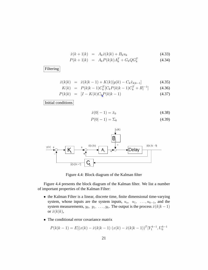
Figure 4.4: Block diagram of the Kalman filter

Figure 4.4 presents the block diagram of the Kalman filter. We list a numberof important properties of the Kalman Filter:

• the Kalman Filter is a linear, discrete time, finite dimensional time-varyingsystem, whose inputs are the system inputs,uo, u1, . . . , uk−1, and thesystem measurements,y0, y1, . . . , yk. The output is the processx(k|k− 1)or x(k|k),

• The conditional error covariance matrix

P (k|k − 1) = E[(x(k)− x(k|k − 1) (x(k)− x(k|k − 1))T |Y k−11 , Uk−1

0

21

is actually independent ofY k−11 , which means that no one set of measure-

ments helps any more than other to eliminate some uncertainty aboutx(k).The filter gain,K(k) is also independent ofY k−1

1 . Because of this, the errorcovarianceP (k|k− 1) and the filter gainK(k) can be computed before thefilter is actually run. This is not generally the case in nonlinear filters.

Some other useful properties will be discussed in the following sections.

4.2 One-step ahead prediction dynamics

Using simultaneously (4.33) and (4.35) the filter dynamics is written in terms ofthe state predicted estimate,

x(k + 1|k) = Ak[I −K(k)Ck]x(k|k − 1) + Bkuk + AkK(k)yk (4.40)

with initial conditionx(0| − 1) = x0 (4.41)

where,

K(k) = P (k|k − 1)CTk [CkP (k|k − 1)CT

k + R]−1 (4.42)

P (k + 1|k) = AkP (k|k − 1)ATk −A(k)K(k)CkP (k|k − 1)A(k)T + GkQGT

k(4.43)

P (0| − 1) = Σo (4.44)

Equation (4.44) may be rewritten differently by replacing the gainK(k) by itsvalue given by (4.42),

P (k+1|k) = AkP (k|k−1)ATk +GkQGT

k−AkP (k|k−1)CTk [CkP (k|k−1)CT

k +R]−1CkP (k|k−1)ATk

(4.45)or else,

P (k+1|k) = AkP (k|k−1)ATk +GkQGT

k−AkK(k)[CkP (k|k−1)CTk +R]KT (k)AT

k .(4.46)

which is a Riccati equation.From the definition of the predicted and filtered errors in (4.16) and (4.18),

and the above recursions, it is immediate that

x(k + 1|k) = Akx(k|k) + Gkwk (4.47)

x(k|k) = [I −K(k)Ck]x(k|k − 1)−K(k)vk (4.48)

22

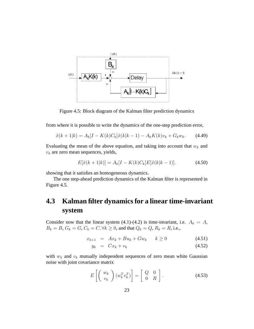
Figure 4.5: Block diagram of the Kalman filter prediction dynamics

from where it is possible to write the dynamics of the one-step prediction error,

x(k + 1|k) = Ak[I −K(k)Ck]x(k|k − 1)− AkK(k)vk + Gkwk. (4.49)

Evaluating the mean of the above equation, and taking into account thatwk andvk are zero mean sequences, yields,

E[x(k + 1|k)] = Ak[I −K(k)Ck]E[x(k|k − 1)]. (4.50)

showing that it satisfies an homogeneous dynamics.The one step-ahead prediction dynamics of the Kalman filter is represented in

Figure 4.5.

4.3 Kalman filter dynamics for a linear time-invariantsystem

Consider now that the linear system (4.1)-(4.2) is time-invariant, i.e.Ak = A,Bk = B, Gk = G, Ck = C,∀k ≥ 0, and thatQk = Q, Rk = R, i.e.,

xk+1 = Axk + Buk + Gwk k ≥ 0 (4.51)

yk = Cxk + vk (4.52)

with wk and vk mutually independent sequences of zero mean white Gaussiannoise with joint covariance matrix

E

[(wk

vk

)(wT

k vTk )

]=

[Q 00 R

]. (4.53)

23

The initial condition,x(0) is Gaussian with meanx0 and covarianceΣ0.The Kalman filter dynamics is obtained by the particularization of the general

time-varying dynamics for the time-invariant situation, i.e.,

x(k + 1|k) = Ax(k|k − 1) + Buk + K(k)[yk − Cxk|k−1] (4.54)

K(k) = P (k|k − 1)CT [CP (k|k − 1)CT + R]−1 (4.55)

P (k +1|k) = AP (k|k−1)AT +GQGT −AK(k)[CP (k|k−1)CT +R]KT (k)A(4.56)

Note that, even though the original system is time-invariant, the Kalman Filter isa time-varying linear system, given that in (4.54) the Kalman gain is a functionof k.

Equation (4.56) is known as a discrete Riccati equation. In the sequel, wediscuss the conditions under which the Riccati equation converges.

Under certain conditions, detailed in the following subsection, the Kalmangain converges to a steady-state value. The corresponding filter is known as thesteady-state Kalman filter.

4.4 Steady-state Kalman filter

Consider the system dynamics (4.51)-(4.52) and assume the following additionalassumptions:

1. The matrixQ = QT > 0, i.e., is a positive definite matrix,

2. The matrixR = RT > 0, i.e., is a positive definite matrix,

3. The pair(A, G) is controllable, i.e.,

rank[G | AG | A2G | . . . | An−1G] = n,

4. The pair(A, C) is observable, i.e.,

rank[CT | AT CT | AT 2

CT | . . . | AT n−1

CT ] = n.

Result 4.4.1 Under the above conditions,

24

1. The prediction covariance matrixP (k|k−1) converges to a constant matrix,

limk→∞

P (k|k − 1) = P

whereP is a symmetric positive definite matrix,P = P T > 0.

2. P is the unique positive definite solution of the discrete algebraic Riccatiequation

P = APAT − APCT [CPCT + R]−1CPAT (4.57)

3. P is independent ofΣ0 provided thatΣ0 ≥ 0.

Proof: see [2].As a consequence of Result 4.4.1, the filter gain in (4.55) converges to

K = limk→∞

K(k) = PCT [CPCT + R]−1 (4.58)

i.e., in steady-state the Kalman gain is constant and the filter dynamics is time-invariant.

4.5 Initial conditions

In this subsection we discuss the initial conditions considered both for the systemand for the Kalman filter. With no loss of generality, we will particularize thediscussion for null control inputs,uk = 0.

SystemLet {

xk+1 = Axk + Gwk, k ≥ 0yk = Cxk + vk

(4.59)

where

E[x0] = x0 (4.60)

Σ0 = E[(x0 − x0)(x0 − x0)T ] (4.61)

and the sequences{vk} and{wk} have the statistical characterization presented inSection 2.

25

Applying the mean value operator to both sides of (4.59) yields

E[xk+1] = AE[xk]

whose solution isE[xk] = Akx0. (4.62)

Thus, if x0 6= 0, {xk} is not a stationary process. Assume that the following hy-pothesis hold:

Hypothesis: x0 = 0The constant variation formula applied to (4.59) yields

x(l) = Al−kx(k) +l−1∑j=k

Al−1−jGwj. (4.63)

Multiplying (4.63) on the right byxT (k) and evaluating the mean value, results:

E[x(l)xT (k)] = Al−kE[x(k)x(k)T ], l ≥ k.

Consequently, forx(k) to be stationary,E[x(l)xT (k)] should not depend onk.EvaluatingE[x(k)x(k)T ] for increasing values ofk we obtain:

E[x(0)x(0)T ] = Σ0 (4.64)

E[x(1)x(1)T ] = E[(Ax(0) + Gw(0))(xT (0)AT + wT (0)GT )] = AΣ0AT + GQGT(4.65)

E[x(2)x(2)T ] = AE[(x(1)x(1)T ]AT + GQGT = A2Σ0A2T

+ AGQGT AT + GQGT(4.66)

from where

E[x(k)x(k)T ] = AE[(x(k − 1)x(k − 1)T ]AT + GQGT . (4.67)

Therefore, the process{xk} is stationary if and only if

Σ0 = AΣ0AT + GQGT .

Remark, however, that this stationarity condition is not required for the applica-tion of the Kalman filter nor it degrades the filter performance.

Kalman filter

26

The filter initial conditions, given, for example, in terms of the one-step pre-diction are:

x(0 | −1) = x0 (4.68)

P (0 | −1) = Σ0, (4.69)

which means that the first state prediction has the same statistics as the initialcondition of the system. The above conditions have an intuitive explanation.Inthe absence of system measurements (i.e., formally at time instantk = −1), thebest that can be said in terms of the state prediction at time instant0 is that thisprediction coincides with the mean value of the random vector that is the systeminitial state.

As will be proved in the sequel, the choice of (4.68) and (4.69) leads to un-biased state estimates for allk. When the values ofx0 andΣ0 are not a prioriknown, the filter initialization cannot reflect the system initial conditions. A pos-sible choice is

x(0 | −1) = 0 (4.70)

P (0 | −1) = P0 = αI. (4.71)

4.6 Innovation Process

The processe(k) = y(k)− y(k|k − 1) (4.72)

is known as the innovation process. It represents the component ofy(k) that can-not be predicted at time instantk− 1. In other others, it represents the innovation,the novelty thaty(k) brings to the system at time instantk. This process has someimportant characteristics, that we herein list.

Property 4.6.1 The innovation process has zero mean.

Prof:

E[e(k)] = E[y(k)− y(k|k − 1)]

= E[Cx(k) + v(k)− Cx(k|k − 1)]

= CE[x(k|k − 1)]

27

given that{vk} is zero mean. For a time-invariant system, the prediction error dy-namics is given by (4.50) that is a homogeneous dynamics. The same conclusionholds for a time-invariant system. Fork = 0, E[x(0| − 1)] = 0 given that

E[x(0| − 1)] = E[x0]− x(0| − 1)

and we choosex(0| − 1) = x0 (see 4.38). Therefore, the mean value of theprediction error is zero, and in consequence, the innovation process has zero mean.

2

The above proof raises a comment relative to the initial conditions chosen forthe Kalman filter. According to (4.50) the prediction error has a homogeneousdynamics, and therefore an initial null error leads to a null error for everyk. Ifx0|−1 6= x0 the initial prediction error is not zero. However, under the conditionsfor which there exists a steady solution for the discrete Riccati equation, the errorassimptotically converges to zero.

Property 4.6.2 The innovation process iswhite.

Proof: In this proof we will consider thatx0|−1 = x0, and thusE[e(k)] = 0, i.e.,the innovation process is zero mean. We want to prove that

E[e(k)eT (j)] = 0

for k 6= j. For simplicity we will consider the situation in whichj = k + 1; thisis not the entire proof, but rather a first step towards it. From the definition of theinnovation process, we have :

e(k) = Cx(k|k − 1) + vk

and thus

E[e(k)eT (k + 1)] = CE[x(k|k − 1)x(k + 1|k)]CT + CE[x(k|k − 1)vTk+1]

+E[vkxT (k + 1|k)]CT + E[vkv

Tk+1] (4.73)

As {vk} has zero mean and is a white process, the second and fourth terms in(4.73) are zero. We invite the reader to replace (4.33) and (4.35) in the aboveequality and to conclude the demonstration.

Property 4.6.3E[e(k)eT (k)] = CP (k|k − 1)CT + R

Property 4.6.4limk→∞

E[e(k)eT (k)] = CPCT + R

28

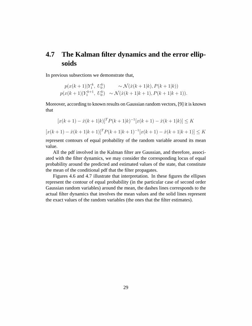
4.7 The Kalman filter dynamics and the error ellip-soids

In previous subsections we demonstrate that,

p(x(k + 1)|Y k1 , Uk

0 ) ∼ N (x(k + 1|k), P (k + 1|k))

p(x(k + 1)|Y k+11 , Uk

0 ) ∼ N (x(k + 1|k + 1), P (k + 1|k + 1)).

Moreover, according to known results on Gaussian random vectors, [9] it is knownthat

[x(k + 1)− x(k + 1|k)]T P (k + 1|k)−1[x(k + 1)− x(k + 1|k)] ≤ K

[x(k + 1)− x(k + 1|k + 1)]T P (k + 1|k + 1)−1[x(k + 1)− x(k + 1|k + 1)] ≤ K

represent contours of equal probability of the random variable around its meanvalue.

All the pdf involved in the Kalman filter are Gaussian, and therefore, associ-ated with the filter dynamics, we may consider the corresponding locus of equalprobability around the predicted and estimated values of the state, that constitutethe mean of the conditional pdf that the filter propagates.

Figures 4.6 and 4.7 illustrate that interpretation. In these figures the ellipsesrepresent the contour of equal probability (in the particular case of second orderGaussian random variables) around the mean, the dashes lines corresponds to theactual filter dynamics that involves the mean values and the solid lines representthe exact values of the random variables (the ones that the filter estimates).

29

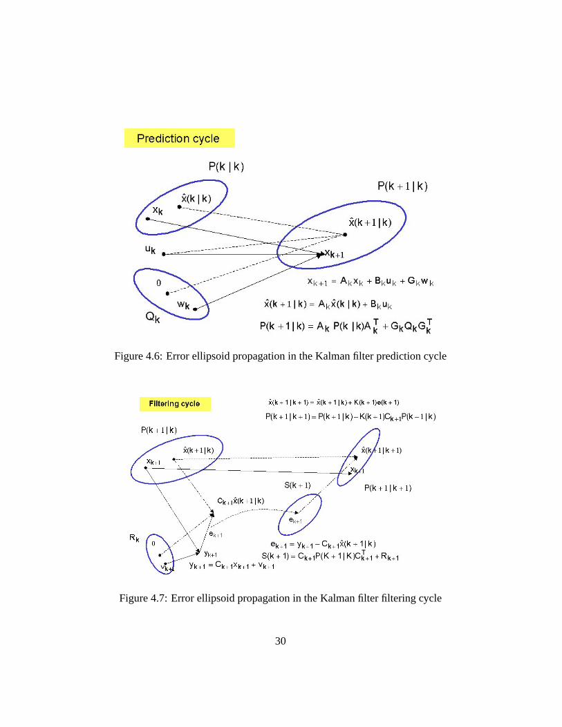
Figure 4.6: Error ellipsoid propagation in the Kalman filter prediction cycle

Figure 4.7: Error ellipsoid propagation in the Kalman filter filtering cycle

30

Chapter 5

The Extended Kalman Filter

In this section we address the filtering problem in case the system dynamics (stateand observations) is nonlinear. With no loss of generality we will consider thatthe system has no external inputs. Consider the non-linear dynamics

xk+1 = fk(xk) + wk (5.1)

yk = hk(xk) + vk (5.2)

where,xk ∈ Rn, fk(xk) : Rn,−→ Rn

yk ∈ Rr hk(xk) : Rn −→ Rr

vk ∈ Rr

wk ∈ Rn

(5.3)

and {vk}, {wk} are white Gaussian, independent random processes with zeromean and covariance matrix

E[vkvTk ] = Rk, E[wke

Tk ] = Qk (5.4)

andx0 is the system initial condition considered as a Gaussian random vector,

x0 ∼ N(x0, Σ0).

Let Y k1 = {y1, y2, . . . , yk} be a set of system measurements. The filter’s goal is

to obtain an estimate of the system’s state based on these measurements.As presented in Section 2, the estimator that minimizes the mean-square error

evaluates the condition mean of the pdf ofxk given Y k1 . Except in very partic-

ular cases, the computation of the conditional mean requires the knowledge of

31

the entire conditional pdf. One of these particular cases, referred in Section 4, isthe one in which the system dynamics is linear, the initial conditional is a Gaus-sian random vector and system and measurement noises are mutually independentwhite Gaussian processes with zero mean. As a consequence, the conditional pdfp(x(k) | Y k

1 ), p(x(k + 1) | Y k1 ) andp(x(k + 1) | Y k+1

1 ) are Gaussian.With the non linear dynamics (5.1)-(5.2), these pdf are non Gaussian. To

evaluate its first and second moments, the optimal nonlinear filter has to propagatethe entire pdf which, in the general case, represents a heavy computational burden.

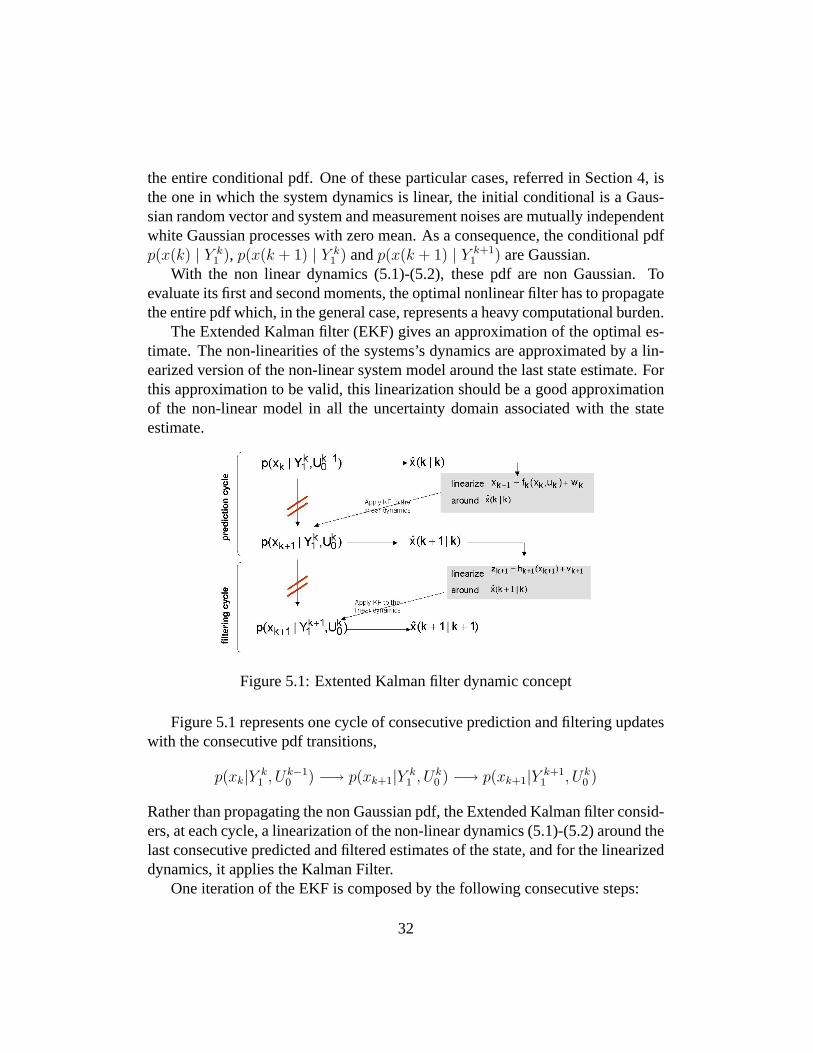
The Extended Kalman filter (EKF) gives an approximation of the optimal es-timate. The non-linearities of the systems’s dynamics are approximated by a lin-earized version of the non-linear system model around the last state estimate. Forthis approximation to be valid, this linearization should be a good approximationof the non-linear model in all the uncertainty domain associated with the stateestimate.

Figure 5.1: Extented Kalman filter dynamic concept

Figure 5.1 represents one cycle of consecutive prediction and filtering updateswith the consecutive pdf transitions,

p(xk|Y k1 , Uk−1

0 ) −→ p(xk+1|Y k1 , Uk

0 ) −→ p(xk+1|Y k+11 , Uk

0 )

Rather than propagating the non Gaussian pdf, the Extended Kalman filter consid-ers, at each cycle, a linearization of the non-linear dynamics (5.1)-(5.2) around thelast consecutive predicted and filtered estimates of the state, and for the linearizeddynamics, it applies the Kalman Filter.

One iteration of the EKF is composed by the following consecutive steps:

32

1. Consider the last filtered state estimatex(k|k),

2. Linearize the system dynamics,xk+1 = f(xk) + wk aroundx(k|k),

3. Apply the prediction step of the Kalman filter to the linearized system dy-namics just obtained, yieldingx(k + 1|k) andP (k + 1|k),

4. Linearize the observation dynamics,yk = h(xk) + vk aroundx(k + 1|k),

5. Apply the filtering or update cycle of the Kalman filter to the linearizedobservation dynamics, yieldingx(k + 1|k + 1) andP (k + 1|k + 1).

Let F (k) andH(k) be the Jacobian matrices off(.) andh(.), denoted by

F (k) = 5fk |x(k|k)

H(k + 1) = 5h |x(k+1|k)

The Extended Kalman filter algorithm is stated below:

Predict Cycle

x(k + 1|k) = fk(x(k|k))

P (k + 1|k) = F (k)P (k|k)F T (k) + Q(k)

Filtered Cycle

x(k + 1|k + 1) = x(k + 1|k) + K(k + 1)[yk+1 − hk+1(x(k + 1|k))]

K(k + 1) = P (k + 1|k)HT (k + 1)[H(k + 1)P (k + 1|k)HT (k + 1) + R(k + 1)]−1

P (k + 1|k + 1) = [I −K(k + 1)H(k + 1)]P (k + 1|k)

It this important to state that the EKF is not an optimal filter, but rathar it isimplemented based on a set of approximations. Thus, the matricesP (k|k) andP (k + 1|k) do not represent the true covariance of the state estimates.

Moreover, as the matricesF (k) andH(k) depend on previous state estimatesand therefore on measurements, the filter gainK(k) and the matricesP (k|k) andP (k + 1|k) cannot be computed off-line as occurs in the Kalman filter.

Contrary to the Kalman filter, the EKF may diverge, if the consecutive lin-earizations are not a good approximation of the linear model in all the associateduncertainty domain.

33

5.1 Derivation of Extended Kalman Filter dynamics

This subsection presents the formal derivation of the EKF dynamics.

Prediction

Assume thatp(xk | Y k1 ) is a Gaussian pdf with meanηn

F1 and covariance

matrixV nF , i.e.,

p(xk | Y k1 ) ∼ N (xk − ηk

F , V kF ) = N (xk − x(k|k), P (k|k)). (5.5)

From the non-linear system dynamics,

xk+1 = fk(xk) + wk, (5.6)

and the Bayes law, the conditional pdf ofxk+1 givenY k1 is given by

p(xk+1 | Y k1 ) =

∫ ∞

−∞p(xk+1 | xk)p(xk | Y k

1 )dxk,

or also,

p(xk+1 | Y k1 ) =

∫ ∞

−∞pwk

(xk+1 − fk(xk))p(xk | Y k1 )dxk (5.7)

where

pwk(xk+1 − fn(xk)) =

1(2π)n/2[detQk]1/2

exp[−12(xk+1 − fk(xk))T Q−1

k (xk+1 − fk(xk))].

(5.8)

The previous expression isnot a Gaussian pdf given the nonlinearity inxk.We will linearizefk(xk) in (5.6) aroundηk

F = x(k | k) negleting higher orderterms, this yielding

fk(xk) ∼= fk(ηkF ) +5fk |ηk

F·[xk − ηk

F ]

=

sk︷ ︸︸ ︷fk(η

kF )−5fk |ηk

F·ηk

F +5 fk |ηkF·xk. (5.9)

where5fk is the Jacobian matrix off(.),

5fk =∂f(x(k))

∂x(k)|ηk

F

1F - refers filtering

34

With this linearization, the system dynamics may be written as:

xk+1 = 5fk |ηkF·xk + wk + [fk(η

kF )−5fk |ηk

F·ηk

F︸ ︷︷ ︸sk

] (5.10)

or, in a condensed format,

xk+1 = 5fk |ηkF·xk + wk + sk (5.11)

Note that (5.11) represents a linear dynamics, in whichsk is known, has a nullconditional expected value and depends on previous values of the state estimate.According to (5.9) the pdf in (5.7) can be written as:

p(xk+1 | Y k1 ) =

∫ ∞

−∞pwk

(xk+1 −5fk |ηkF·xk − sk) · p(xk | Y k

1 )dxk

=∫ ∞

−∞N (xk+1 −5fk |ηk

F·xk − sk, Qk) · N (xk − ηk

F , V kF )dxk

=∫ ∞

−∞N (xk+1 − sk −5fk |ηk

F·xk, Qk)N (xk − ηk

F , V kF )dxk (5.12)

To simplify the computation of the previous pdf, consider the following variabletransformation

zk = 5fk · xk. (5.13)

where we considered, for the sake of simplicity, the simplified notation5fk torepresent5fk |ηk

F.

Evaluating the mean and the covariance matrix of the random vector (5.13)results:

E[yk] = 5fk · E[xk] = 5fk · ηkF (5.14)

E[ykyTk ] = 5fk · V k

F · 5fTk . (5.15)

From the previous result, the pdf ofxk in (5.5) may be written as:

N (xk − ηkF , V k

F ) =1

(2π)n/2(detV kF )1/2

exp[−12(xk − ηk

F )T (V kF )−1(xn − ηk

F )] =

1(2π)n/2(detV k

F )1/2exp[−1

2(5fkxk −5fk · ηk

F )T (5fkF )−T (V k

F )−1(5fkF )−1(5fkxk −5fkηk

F )] =

1(2π)n/2(detV k

F )1/2exp[−1

2(5fkxk −5fkηk

F )T (5fk · V kF 5 fT

k )−1(5fkxk −5fkηkF )] =

= det5 fk ·1

(2π)n/2(det5 fkV kF 5 fT

k )n/2

exp[−12(5fkxk −5fkηk

F )T (5fkV kF 5 fT

k )−1(5fkxk −5fkηkF )].

35

We thus conclude that

N (xk − ηkF , V k

F ) = det5 fk · N (5fkxk −5fkηkF ,5fkV

kF 5 fT

k ). (5.16)

Replacing (5.16) in (5.12) yields:

p(xk+1 | Y k1 ) =

=∫∞−∞N (xk+1 − sk −5fkxk, Qk)N (5fkxk −5fkηk

F ,5fkV kF 5 fT

k )d(5fk · xk)

= N (xk+1 − sk, Qk) ?N (xk+1 −5fk · ηkF ,5fkV k

F 5 fTk )

where? represents the convolution of the two functions. We finally conclude that,

p(xk+1 | Y k1 ) = N (xk+1 −5fk |ηk

F·ηk

F − sk, Qk +5fk |ηkF

V kF 5 fk |Tηk

F(5.17)

We just conclude that,

if p(xk | Zk1 ) is a Gaussian pdf with

1. meanηnF ,

2. covariance matrixV nF

then, the linearization of the dynamics aroundηnF yieldsp(xk+1 | Zk

1 ), which isa Gaussian pdf with

1. meanηk+1P

2. covariance matrixV k+1P

whereηk+1

P = 5fk |ηkF·ηk

F + fk(ηkF )−5fk |ηk

F·ηk

F (5.18)

or else, given the value ofsk given in (5.10), can be simplified to

ηk+1P = fk(η

kF ) (5.19)

V k+1P = Qk +5fk |ηk

F·V k

F · 5fTk |ηk

F. (5.20)

These values are taken as the predicted state estimate and the associated co-variance obtained by the EKF, i.e.,

x(k + 1|k) = ηk+1P (5.21)

P (k + 1|k) = = V k+1P , (5.22)

representing the predicted dynamics,

36

x(k + 1|k) = fk(x(k|k)

P (k + 1|k) = 5fk |ηkF·P (k|k) · 5fT

k |ηkF

Filtering

In the filtering cycle, we use the system measurement at time instantk + 1,yk+1 to update the pdfp(xk+1 | Y k

1 ) as represented

p(xk+1 | Y k1 )

yk+1−→ p(xk+1 | Y k+11 )

According to Bayes law,

p(xk+1 | Y k+11 ) =

p(Y k1 )

p(Y k+11 )

· [p(yk+1 | xk+1) · p(xk+1 | Y k1 )]. (5.23)

Given thatyk+1 = hk+1(xk+1) + vk+1, (5.24)

the pdf ofyk+1 conditioned on the statexk+1 is given by

p(yk+1 | xk+1) =1

(2π)r/2(detRk+1)1/2exp[−1

2(yk+1−hk+1(xk+1))T R−1

k+1(yk+1−hk+1(xk+1))].

(5.25)

With a similar argument as the one used on the prediction cycle, the previous pdfmay be simplified through the linearization of the observation dynamics.

Linearizinghk+1(xk+1) aroundηk+1P and neglecting higher order terms results

hk+1(xk+1) ' hk+1(ηk+1P ) +5h |ηk+1

P(xk+1 − ηk+1

P ), (5.26)

and so the system observation equation may be approximated by,

yk+1 ' 5h |ηk+1P

·xk+1 + vk+1 + rk+1 (5.27)

withrk+1 = hk+1(η

k+1P )−5h |ηk+1

P·ηk+1

P . (5.28)

being a known term in the linearized observation dynamics, (5.27). After thelinearization around the predicted state estimate - that corresponds toηk+1

P =xk+1|k (see (5.21), - the observation dynamics may be considered linear, and thecomputation ofp(yk+1 | xk+1) in (5.25) is immediate. We have,

p(yk+1 | xk+1) = N (yk+1 − rk+1 −5hk+1 |ηk+1P

·xk+1, Rk+1). (5.29)

37

Expression (5.29) may be rewritten as:

p(yk+1 | xk+1) = N (5hk+1 |ηk+1P

·xk+1 + rk+1 − yk+1, Rk+1). (5.30)

Using a variable transformation similar to the one used in the prediction cycle, theprevious pdf may be expressed as

p(xk+1 | Y k1 ) = det5h |ηk+1

PN (5hk+1 |ηk+1

P·xk+1−5hk+1 |ηk+1

P·ηk+1

P ,5hk+1Vk+1P 5hT

k+1)(5.31)

Multiplying expressions (5.30) and (5.31) as represented in the last product in(5.23) yields:

p(yk+1|xk+1).p(xk+1|Y k1 ) ∼ N (5hk+1 |ηk+1

P·xk+1 − µ, V ) (5.32)

where the mean and covariance matrix are given by:

µ = 5hk+1Vk+1P 5 hT

k+1(5hk+1Vk+1P 5 hT

k+1 + Rk+1)−1[−rk+1 + yk+1]

+Rk+1(5hk+1Vk+1P 5 hT

k+1 + Rk+1)−1 5 hk+1 · ηk+1

P , (5.33)

V = 5hk+1Vk+1P 5 hT

k+1(5hk+1Vk+1P 5 hT

k+1 + Rk+1)−1Rk+1. (5.34)

Replacing in (5.33) the expression (5.28) we obtain:

µ = 5hk+1Vk+1P 5 hT

k+1(5hk+1Vk+1T 5 hT

k+1 + Rk+1)−1 (5.35)

[−hk+1(ηk+1P ) +5hk+1 · ηk+1

P + zk+1]

+Rk+1(5hk+1Vk+1P 5 hT

k+1 + Rk+1)−1 5 hk+1ηk+1P

= 5hk+1ηk+1P +5hk+1V

k+1P 5 hT

k+1(5hk+1Vk+1P 5 hT

k+1 + Rk+1)−1[yk+1 − hk+1(ηk+1P )] ·(5.36)

V = 5hk+1Vk+1P 5 hT

k+1(5hk+1Vk+1P 5 hT

k+1 + Rk+1)−1Rk+1 (5.37)

where we use the short notation

5hk+1 = 5hk+1 |ηk+1P

. (5.38)

Note that (5.32) expresses the pdf of5hk+1 |ηk+1P

·xk+1 and not that ofxk+1

as desired. In fact, the goal is to evaluate the mean and covariance matrix in

N (xk+1 − µ1, V1). (5.39)

Note that (5.32) can be obtained from (5.39). We know that:

N (xk+1 − µ1, V1) = det5 hk+1 · N (5hk+1xk+1 −5hk+1µ1,5hk+1V1 5 hTk+1)

= det5 hk+1N (5hk+1xk+1 − µ, V ), (5.40)

38

whereµ andV are given by (5.33) and (5.34).Comparing (5.40) with (5.40) yields:

5hk+1µ1 = 5hk+1ηk+1P +5hk+1V

k+1P 5 hT

k+1(5hk+1Vk+1P 5 hT

k+1 + Rk+1)−1[yk+1 − hk+1(ηk+1P )]

µ1 = ηk+1P + V k+1

P 5 hTk+1(5hk+1V

k+1P 5 hT

k+1 + Rk+1)−1[yk+1 − hk+1(ηk+1P )].

We thus conclude that:

ηk+1F = ηk+1

P + V k+1P 5 hT

k+1(5hk+1Vk+1P 5 hT

k+1 + Rk+1)−1[yk+1 − hk+1(η

k+1P )].

(5.41)Comparing (5.40) and (5.40) in terms of the covariance matrices, yields:

V = 5hk+1V1 5 hTk+1. (5.42)

Replacing in this expression V by its value given by (5.37) result,

V = 5hk+1Vk+1P 5 hT

k+1(5hk+1Vk+1P 5 hT

k+1 + Rk+1)−1Rk+1

= 5hk+1Vk+1F 5 hT

k+1

that has to be solved relative toV k+1F . From the above equalities, we successively

obtain:

5hk+1Vk+1P 5 hT

k+1 = 5hk+1Vk+1F 5 hT

k+1R−1k+1(5hk+1V

k+1P 5 hT

k+1 + Rk+1)

= 5hk+1Vk+1F 5 hT

k+1R−1k+1 5 hk+1V

k+1P 5 hT

k+1 +5hk+1Vk+1F 5 hT

k+1

or else,

V k+1P = V k+1

F 5 hTk+1R

−1k+1 5 hk+1V

k+1P + V k+1

F

V k+1P = V k+1

F [I +5hTk+1R

−1k+1 5 hk+1V

k+1P ]

V k+1F = V k+1

P [I +5hTk+1R

−1k+1 5 hk+1V

k+1P ]−1.

Using the lemma of the inversion of matrices,

V k+1F = V k+1

P [I −5hTk+1R

−1k+1(I +5hk+1V

k+1P 5 hT

k+1R−1k+1)

−1 5 hk+1Vk+1P ]

= V k+1P [I −5hT

k+1[Rk+1 +5hk+1Vk+1P 5 hT

k+1]−1 5 hk+1V

k+1P ]

V k+1F = V k+1

P − V k+1P 5 hT

k+1[Rk+1 +5hk+1Vk+1P 5 hT

k+1]−1 5 hk+1V

k+1P

(5.43)Therefore, if we consider thatp(xk+1|Y k

1 ) is a Gaussian pdf, have accessto the measurementyk+1 and linearize the system observation dynamics around

39

ηk+1P = x(k + 1|k) we obtain a Gaussian pdfp(xk+1 | Y k+1

1 ) with meanηk+1F and

covariance matrixV k+1F given by (5.41) and (5.43), respectively.

Finally, we summarize the previous results and interpret the Extended Kalmanfilter as a Kalman fiter applied to a linear time-varying dynamics.

Let:

ηk+1P = x(k + |k)

V k+1P = P (k + 1|k)

ηk+1F = x(k + 1|k + 1)

V k+1F = P (k + 1|k + 1)

and consider

5fk |ηkF

= 5fk |x(k|k)= F (k)

5hk+1 |ηk+1P

= 5h |x(k+1|k)= H(k + 1)

s(k) = fk(x(k|k))− F (k) · x(k|k)

r(k + 1) = hk+1(x(k + 1|k))−H(k + 1) · x(k + 1|k).

Assume the linear system in whose dynamics the just evaluated quantities areincluded.

x(k + 1) = F (k)x(k) + wk + s(k) (5.44)

y(k + 1) = H(k + 1)x(k + 1) + vk+1 + r(k + 1) (5.45)

wherewk andvk+1 are white Gaussian noises,s(k) andr(k) are known quantitieswith null expected value.

The EKF applies the Kalman filter dynamics to (5.44)-(5.45), where the ma-tricesF (k) andH(k) depend on the previous state estimates, yielding

x(k + 1|k) = fk(x(k|k))

x(k + 1|k + 1) = x(k + 1|k) + K(k + 1)[yk+1 − hk+1(x(k + 1|k))]

whereK(k + 1) is the filter gain and

K(k + 1) = P (k + 1|k)HT (k + 1)[H(k + 1)P (k + 1|k)HT (k + 1) + R(k + 1)]−1

P (k + 1|k) = F (k)P (k|k)FT (k) + Q(k)P (k + 1|k + 1) = P (k + 1|k)− P (k + 1|k)HT (k + 1)

[H(k + 1)P (k + 1|k)HT (k + 1) + R(k + 1)]−1H(k + 1)P (k + 1|k)(5.46)

40

Expression (5.46) may be rewritten as:

P (k + 1|k + 1) = P (k + 1|n)× (5.47)

×[I − P (k + 1|n)HT (k + 1)[H(k + 1) + P (k + 1|k)HT (k + 1) + Rk+1]−1H(k + 1)](5.48)

P (k + 1|k + 1) = [I −K(k + 1)H(k + 1)]P (k + 1|k) (5.49)

41

Bibliography

[1] Michael Athans, ”Dynamic Stochastic Estimation, Prediction and Smooth-ing,” Series of Lectures, Spring 1999.

[2] T. Kailath, “Lectures Notes on Wiener and Kalman Filtering,” Springer-Verlag, 1981.

[3] Thomas Kailath, Ali H. Sayed, Babak Hassibi, ” Linear Estimation,” Pren-tice Hall, 2000.

[4] Peter S. Maybeck, ”The Kalman Filter: An Introduction to Concepts,” inAutonomous Robot Vehciles, I.J. Cox, G. T. Wilfong (eds), Springer-Verlag,1990.

[5] J. Mendel, “Lessons in Digital Estimation Theory”, Prentice-Hall, 1987.

[6] K. S. Miller, “Multidimensional Gaussian Distributions,” John Wiley &Sons, 1963.

[7] J. M. F. Moura, “Linear and Nonlinear Stochastic Filtering,” NATO Ad-vanced Study Institute, Les Houches, September 1985.

[8] A. Papoulis, “Probability, Random Variables and Stochastic Processes,”McGraw-Hill, 1965.

[9] M. Isabel Ribeiro, “Gaussian Probability Density Functions: Properties andError Characterization,” Institute for Systems and Robotics, Technical Re-port, February 2004.

[10] H. L. Van Trees, “Detection, Estimation and Modulation Theory,” John Wi-ley & Sons, 1968.

42

ERRATA  

 

The equation (4.37) has an error. The correct version is 

P (k|k )= [ I ‐K (k )C ]P (k|k ‐1 )  

Thanks to Sergio Trimboli that pointed out the error in a preliminary version 

 

23.March.2008