Variance Estimation with Hot Deck Imputation: A Simulation ... · PDF fileknife method (Rao and Shao 1992), and multiple imputation (Rubin 1987). Each method has been evaluated theoretically

Catalogue no. 12-001-XIE

SurveyMethodology

December 2005

How to obtain more information

Specific inquiries about this product and related statistics or services should be directed to: Business Survey Methods Division,Statistics Canada, Ottawa, Ontario, K1A 0T6 (telephone: 1 800 263-1136).

For information on the wide range of data available from Statistics Canada, you can contact us by calling one of our toll-freenumbers. You can also contact us by e-mail or by visiting our website.

National inquiries line 1 800 263-1136National telecommunications device for the hearing impaired 1 800 363-7629Depository Services Program inquiries 1 800 700-1033Fax line for Depository Services Program 1 800 889-9734E-mail inquiries [email protected] www.statcan.ca

Information to access the product

This product, catalogue no. 12-001-XIE, is available for free. To obtain a single issue, visit our website at www.statcan.ca andselect Our Products and Services.

Standards of service to the public

Statistics Canada is committed to serving its clients in a prompt, reliable and courteous manner and in the official language oftheir choice. To this end, the Agency has developed standards of service that its employees observe in serving its clients. Toobtain a copy of these service standards, please contact Statistics Canada toll free at 1 800 263-1136. The service standardsare also published on www.statcan.ca under About Statistics Canada > Providing services to Canadians.

Statistics CanadaBusiness Survey Methods Division

SurveyMethodology

December 2005

Note of appreciation

Canada owes the success of its statistical system to a long-standing partnership between Statistics Canada, the citizens of Canada, its businesses, governments and other institutions. Accurate and timely statistical information could not be produced without their continued cooperation and goodwill.

May 2006

Catalogue no. 12-001-XIEISSN 1492-0921

Frequency: semi-annual

Ottawa

Cette publication est disponible en français sur demande (no 12-001-XIF au catalogue).

Published by authority of the Minister responsible for Statistics Canada © Minister of Industry, 2006 All rights reserved. The content of this electronic publication may be reproduced, in whole or in part, and by any means, without further permission from Statistics Canada, subject to the following conditions: that it be done solely for the purposes of private study, research, criticism, review or newspaper summary, and/or for non-commercial purposes; and that Statistics Canada be fully acknowledged as follows: Source (or “Adapted from”, if appropriate): Statistics Canada, year of publication, name of product, catalogue number, volume and issue numbers, reference period and page(s). Otherwise, no part of this publication may be reproduced, stored in a retrieval system or transmitted in any form, by any means—electronic, mechanical or photocopy—or for any purposes without prior written permission of Licensing Services, Client Services Division, Statistics Canada, Ottawa, Ontario, Canada K1A 0T6.

Vol. 31, No. 2, pp. 151-159 Statistics Canada, Catalogue No. 12-001

Variance Estimation with Hot Deck Imputation: A Simulation Study of Three Methods

J. Michael Brick, Michael E. Jones, Graham Kalton and Richard Valliant 1

Abstract

Complete data methods for estimating the variances of survey estimates are biased when some data are imputed. This paper uses simulation to compare the performance of the model-assisted, the adjusted jackknife, and the multiple imputation methods for estimating the variance of a total when missing items have been imputed using hot deck imputation. The simulation studies the properties of the variance estimates for imputed estimates of totals for the full population and for domains from a single-stage disproportionate stratified sample design when underlying assumptions, such as unbiasedness of the point estimate and item responses being randomly missing within hot deck cells, do not hold. The variance estimators for full population estimates produce confidence intervals with coverage rates near the nominal level even under modest departures from the assumptions, but this finding does not apply for the domain estimates. Coverage is most sensitive to bias in the point estimates. As the simulation demonstrates, even if an imputation method gives almost unbiased estimates for the full population, estimates for domains may be very biased.

1. J. Michael Brick, Michael E. Jones and Graham Kalton, Westat, 1650 Research Boulevard, Rockville, MD 20850; Richard Valliant, University of

Michigan, 1218 Lefrak Hall, College Park, MD 20742.

Key Words: Adjusted jackknife; Domain estimation; Model-assisted variance estimation; Multiple imputation;

Nonresponse.

1. Introduction

Imputation is frequently used in survey research to assign values for missing item responses, thereby producing complete data sets for public use or general analysis. It is well-recognized that treating imputed values as observed values results in downwardly biased variance estimates for the survey estimates. As a result, confidence intervals have lower than nominal levels. The biases in the variance estimates tend to increase with the item nonresponse rate and can be substantial when that rate is high.

Three methods of variance estimation that have been developed for use with imputed data are studied here: a model-assisted method (Särndal 1992), an adjusted jack-knife method (Rao and Shao 1992), and multiple imputation (Rubin 1987). Each method has been evaluated theoretically and by simulation methods, primarily under conditions consistent with the assumptions of the methods. This paper uses simulation to compare the three methods under the same experimental conditions in which some of the assump-tions required by the methods do not hold. The goal is to examine the relative performances of the methods in situations that are likely to occur in practice. Other simu-lation studies of variance estimation methods with imputed data have generally been more limited. Even the more extensive simulation study by Lee, Rancourt, and Särndal (2001) was based on small populations and it did not include multiple imputation.

A single-stage disproportionate stratified sample selected from a real population data set is used to evaluate these variance estimation methods in a realistic setting. The imputed values are assigned using a hot deck imputation method, one of the most popular methods of imputation in survey research. Since hot deck imputation is a form of regression imputation (Kalton and Kaspryzk 1986), re-stricting the simulation study to the hot deck is not a crucial feature for examining the implications for variance estima-tion. We study estimation for both full population and domain totals. For the domain estimates, the domain indi-cator is assumed to be known for all sample members.

Three different combinations of missing data mecha-nisms and hot deck cell formation are used in the simula-tions to assess the performance of the variance estimation methods under conditions that violate the assumptions of the methods to varying degrees. The three variance estimation methods we study all assume that data are randomly missing in each hot deck cell and the model-assisted (MA) and multiple imputation (MI) methods also assume that a simple model with common mean and variance holds in each cell. Studying the robustness of the variance estimation methods is an important feature of the simulation because in practice the assumptions underlying the methods will almost never be fully satisfied.

The next section briefly describes three variance estima-tion methods with hot deck imputed data. The third section outlines the study population, the sample design used in the simulations, and the methods used to generate the missing

4 Brick, Jones, Kalton and Valliant: Variance Estimation with Hot Deck Imputation

Statistics Canada, Catalogue No. 12-001

data and implement the hot deck imputations. The fourth section gives the results of the simulations. The last section gives some conclusions about the methods and their applica-bility.

2. Description of the Variance Estimation Methods

We denote the full sample by A, the subset that responds to an item by ,RA and the subset that does not respond by

.MA For the imputations the units are divided into hot deck cells indexed by ,,,1 Gg K= where the subset of Rgn respondents in cell g is ,RgA and the subset of non-respondents is .MgA For each unit with a missing value, the hot deck method consists of randomly selecting a respondent from within the same hot deck cell to be the donor of the imputed value.

With hot deck imputation, donors are often selected within a cell by simple random sampling with replacement (srswr), by simple random sampling without replacement, or by sampling with probabilities proportional to the survey weights with replacement (ppswr). Since the simulation results obtained using the srswr and the ppswr methods are very similar, only the results for the ppswr method – termed the weighted hot deck – are presented here. The imputed estimator of a population total is ∑ ∈ +=θ

RAi iiI ywˆ ∑ ∈

∗MAi ii yw , where iw is the survey weight, iy is the

reported value and ∗iy is the imputed value for unit i in the

nonrespondent set. 2.1 Model-Assisted Variance Estimation

The model-assisted (MA) approach with hot deck imputation assumes that data are randomly missing within the hot deck cells and that a model for the generation of the y’s holds. A natural model for use with hot deck imputation is that the iy ’s are independently and identically generated within the hot deck cells, i.e., ),( 2iid

~ gggiy σμ for cell g. Inferences from the model-assisted approach depend on the validity of the model assumptions.

Särndal (1992) decomposed the total variance of the imputed estimator into three components denoted by

,, IMPSAM VV and .MIXV The estimators used for these com-ponents in the simulations are those given in Brick, Kalton, and Kim (2004). The MA variance estimator is the sum of the component estimates: ++= IMPSAMMA

ˆˆˆ VVV .ˆ2 MIXV The

IMPV̂ and MIXV̂ estimators require an estimator of the element variance in each hot deck cell. Since the simu-lations showed little difference between weighted and un-weighted estimators only the weighted estimator of 2

gσ is discussed, that is ×−−=σ ∑− 212 )()1(ˆ

RgA RgiiRgRgg yywnn ,)( 1−∑

RgA iw with .)( 1−∑∑=RgRg A iA iiRg wywy

2.2 Adjusted Jackknife Variance Estimation The Rao and Shao (1992) adjusted jackknife (AJ)

variance estimator for a stratified sample with imputations and ignorable finite population correction factors ( fpc’s) is

,)ˆˆ(1

)ˆ(ˆ 2)(

11I

kIh

h

hn

k

L

hI n

nV

h

θ−θ−=θ ∑∑==

where hn is the number sampled in stratum h,

∑ ∑ ∑= ∈

∗

∈ ⎪⎭

⎪⎬⎫

⎪⎩

⎪⎨⎧

−++=θG

g AhiRg

kRghj

khj

Ahjhi

khi

kIh

Rg Mg

yyywyw1 )(

)()(

)(

)()( )ˆ(ˆ

is the adjusted estimator when unit k is omitted,

,

,ˆ

)()(

)(

)(

)(

)(

)(

hiAhi

hihiAhi

Rg

khi

Ahihi

khi

Ahi

kRg

wywy

wywy

RgRg

RgRg

∑∑

∑∑

∈∈

∈∈

=

=

)(khiw is the weight for unit hi adjusted to account for the

omission of unit k. The notation (hi) ∈ B denotes unit i in stratum h is part of set B. This procedure requires the computation of ∑ hn replicate estimates, .ˆ )(k

Ihθ A commonly used strategy to reduce the computations is to combine units into variance strata (e.g., see Rust and Rao 1996). Let ∗h denote a combined variance stratum and k a group of sample units within the combined stratum. All sampled units are assigned to one of the groups. Then, the grouped adjusted jackknife variance estimator is

∑∑∗

∗

∗

∗

∗

=θ−θ=

h

n

kI

kIh

h

khAJ

h

n

nV

1

2)()( ,)ˆˆ(ˆ

where ∗hn is the number of sample units in combined

variance stratum )(

,kh

nh ∗∗ is the number of units retained in

stratum ∗h when units in group k are deleted and, corresponding to )()( ˆ,ˆ k

Ihk

Ih ∗θθ is the adjusted imputed estimate for the full population when units in group k in stratum ∗h are deleted. The retained units from design stratum h that are in combined variance stratum ∗h are assigned replicate weights of .)( 1

)()(

ihkhhkih

wnnw ∗∗∗∗−=

The AJ method assumes a uniform response probability model within each hot deck cell but, unlike the MA method, it does not require distributional assumptions. Under the uniform response probability model without distributional assumptions, a weighted hot deck is needed to produce unbiased imputed estimates.

In developing the theory for the AJ method, Rao and Shao (1992) assume that fpc’s are ignorable. However, the fpc’s are not negligible in some strata in the simulations, ranging from about 0.05 to 0.24. Shao and Steel (1999) and Lee, Rancourt, and Särndal (1995) provide methods for accounting for nonnegligible fpc’s. The Lee, Rancourt, and Särndal (1995) fpc adjustment was applied in the simu-lations because of its ease of implementation. Without the

Survey Methodology, December 2005 5


fpc adjustment, the AJ variance estimator substantially overestimated the variances in the simulations. 2.3 Multiple Imputation

Multiple imputation (MI) is described in detail in Rubin (1987) and Little and Rubin (2002). The summary here relates to its application with hot deck imputation. As with the model-assisted approach, within the hot deck cells re-sponses are assumed to be missing randomly and the y’s are assumed to be independent random variables with a com-mon mean and variance. For each unit that has a missing value, M values are imputed, creating M completed data sets.

To avoid underestimation of variances with the MI method, the hot deck method needs to be modified. Rubin and Schenker (1986) proposed the approximate Bayesian bootstrap (ABB) for simple random sampling with hot deck imputation for use with the MI method. The ABB was modified for the simulations to accommodate sampling donors by ppswr. In the simulations a donor pool for the ABB was created in each cell by selecting respondents with replacement with probabilities proportional to .iw (There is no literature that discusses the application of ABB methods with unequal weights. In hindsight, an unweighted ABB might have been preferable. The use of an unweighted ABB with a ppswr hot deck yields unbiased point estimates of population totals under the response probability model).

3. Design of the Simulation Study 3.1 Description of the Study Population and Sample Design

The sampling frame for the simulations is a subset of the file of public school districts extracted from the 1999 – 2000 Common Core of Data (CCD) compiled by the U.S. National Center for Education Statistics. The final frame consists of 11,941 districts.

The sample design used in the simulations is a stratified simple random sample of 1,020 school districts. Twelve strata were created by cross-classifying four categories of number of students (district size) by three categories of the percentage of students at or below the poverty level (poverty status). The strata and number of districts in the frame are given in Table 1. The table also gives the stratum sample sizes and sampling rates used in the simulations.

The table also contains the stratum means and standard deviations for the two study variables, the number of students in the district and the number of districts that include pre-kindergarten as the lowest grade. These study variables were chosen because they are typical of many estimates computed from this type of design.

In addition to the full population estimates we computed the two study estimates for two domains, defined as districts located in the Northeast region and those in nonmetropolitan areas. The means for these domains are substantially different from the full population means for both study variables. 3.2 Missing Data Mechanisms and Imputation Methods

By construction, information on the two study variables is available for all districts in the sampling frame. To create missing values, response indicators were assigned to sampled units within “response cells”. In some cases the response cells are the sampling strata, termed STR cells, whereas in other cases they are what are termed HD cells. The HD cells were defined by the cross-classification of four geographic regions and a fourfold categorization of the number of full time equivalent teachers in the district. The HD cells are somewhat correlated with the sampling strata, but each cell contains units from more than one stratum.

Table 1

Stratum Definitions, Population Counts, Sample Sizes, Sampling Rates, Means and Standard Deviations of Number of Students and Proportions of Districts with Pre-Kindergarten

Number of students Stratum

District size

Poverty status

Nh

nh

Sampling rate Mean Std. dev.

Proportion with pre-kindergarten

1 1 1 615 32 0.0520 270.0 155.0 0.44 2 1 2 1,147 59 0.0514 263.3 175.0 0.49 3 1 3 1,292 66 0.0511 243.5 142.5 0.49 4 2 1 1,720 111 0.0645 1,607.2 837.0 0.44 5 2 2 2,305 149 0.0646 1,429.7 784.1 0.52 6 2 3 1,893 122 0.0644 1,427.8 788.8 0.63 7 3 1 692 75 0.1084 4,695.3 1,360.6 0.35 8 3 2 579 63 0.1088 4,728.5 1,365.0 0.51 9 3 3 527 57 0.1082 4,591.8 1,380.3 0.63

10 4 1 342 83 0.2427 16,003.4 12,670.2 0.51 11 4 2 449 110 0.2450 17,577.3 14,246.7 0.58 12 4 3 380 93 0.2447 19,331.8 16,142.7 0.68

Total 11,941 1,020 3,237.9 6,770.5 0.52



Within a given response cell, sampled units were assigned at random to be missing or nonmissing at a specified rate. For each type of response cell, three schemes for assigning rates of missingness were chosen. In two of the schemes, the rates of missingness varied across the response cells, whereas in the other scheme the rate was constant across the cells.

The simulations were conducted by first drawing a stratified simple random sample using the stratum sample sizes in Table 1. Once the sample was selected, response status (respondent/nonrespondent) was randomly assigned to each sampled unit according to the given response scheme. For the MA and AJ methods, the weighted hot deck imputation procedures described earlier were used to impute for missing values. For the MI method, a donor pool was first created using the weighted ABB, and weighted hot decks were then used to impute for each of the M = 5 imputed data sets. The estimated total numbers of students and districts with pre-kindergarten were computed for the simulated sample with imputed values, and variance estimates were computed for these estimates using the three variance estimation methods. (If the estimated variance could not be computed in a particular simulation run or the sample size in a cell was less than 2, then that sample was deleted. The maximum number of deleted samples across all the simulations of 10,000 runs each was 2 for the MA method and 28 for the AJ (only one run had 28 AJ samples deleted; the next largest number was 3). The AJ method was based on three combined variance strata and 40 groups of units per stratum for a total of 120 replicates. The three combined strata, formed from strata having about the same fpc, consisted of strata 1 – 6, 7 – 9, and 10 – 12. As a check of the grouping, we verified that the grouped jackknife variance procedure gave essentially the same average variance estimates and confidence interval coverage rates as the ungrouped jackknife in the case of complete response. The entire process was repeated 10,000 times for each response scheme.

A feature of the design of the simulation is that the means for the two domains considered often differ substantially from the full population means by strata and HD cells. A key point for the domain estimates is that imputations were made by selecting donors from all the respondents in a hot deck cell, without specifically recognizing the domain as might be done in practice for some domains. After impu-tations were made for the full sample, the estimated total for a domain was estimated by ∑ ∑∈ ∈+δ=θ

R MAi AjiiiI ywˆ ∗δ jjj yw where 1=δi if unit i is in the domain and 0 if not.

Three of the four possible combinations of response mechanism (STR or HD cells) and hot deck cell formation (STR or HD cells) were studied in the simulations. We refer to these combinations as STR/STR, HD/HD, and STR/HD,

where the first set of letters identifies the response mechanism and the second set identifies the type of hot deck cell. The three sets of response rates were 0.2 to 0.6 spaced evenly across the response cells, a constant 0.7 in all cells, and 0.6 to 0.9 spread evenly across the cells. The three combinations of response/hot deck cells with the three sets of response rates generated nine separate simulation schemes for each estimate. 3.3 Assumptions for Models of Response and Population Structure

There are two models involved in the simulations. The population model assumes that the y values within each hot deck cell are independent and have the same expected value. The response model assumes that there is a uniform response probability within each hot deck cell. If both models hold, then the use of either an unweighted or a weighted hot deck will lead to an unbiased estimate of the overall population total. However, if only the response model is assumed, then the use of a weighted hot deck is needed to produce an unbiased estimate of the overall population total. Since the weighted hot deck is used in the simulations, only the response probability model needs to be satisfied for unbiased point estimation of the overall popu-lation total. The response probability model holds for all the STR/STR and HD/HD combinations and for the STR/HD combination with a constant response rate; however, it does not hold for the other two STR/HD combinations. The AJ theory for variance estimation of population totals was developed assuming only the response probability model. The MA and MI theories assume that both models hold.

Reliance on only the response probability model and the weighted hot deck to produce unbiased estimates of population totals does not in general extend to estimates of domain totals. When domains cut across hot deck cells, it is necessary to invoke a population model that assumes that the expected value of the domain values is the same as that of the nondomain values in each hot deck cell. However, if the hot deck cells are defined such that each domain comprises the full population in a subset of the hot deck cells, then the situation for point and variance estimation is the same as stated above for overall population totals.

The simulation schemes were generally constructed so that the hot deck cells do not incorporate the domains in order to reflect the practical consideration that it is essentially impossible to incorporate all domains in an imputation scheme. Specifically, in the simulations the districts in the Northeast (NE) region and districts in nonmetropolitan statistical areas (NMSA) are unrelated to the stratum definitions in Table 1 (which are used as hot deck cells in some cases). Also, districts in the NMSA domain can be found in all HD cells. However, the NE



domain is a subset of four of the HD cells. Thus, the definition of the HD cells is more consistent with estimating NE domain totals than NMSA domain totals. 3.4 Summary Statistics

The relative bias of a point estimate is estimated by ,/)ˆ(bias)ˆ(relbias NII θθ=θ where /)ˆ()ˆ(bias NIssI θ−θ=θ ∑

Isθ̂,000,10 is the estimate from sample s, and Nθ is the finite population parameter. The empirical variance of Iθ̂ is ,000,10/)ˆ()ˆ(Var 2∑ θ−θ=θ s IIsI where ∑ θ=θ s IsI /ˆ 10,000. The average variance estimate for a particular method is ∑= s svv ,000,10/ where sv is the estimated variance for simulation run s.

The percentages of intervals that include Nθ are based on the nominal 95 percent confidence intervals

)ˆˆ( 2/1VtI ±θ computed for each of the 10,000 simulations for each simulation scheme. An issue to consider here is the precision of the variance estimates from a disproportionate stratified sample design and its impact on whether normal approximation or t intervals should be used to calculate confidence intervals. We found that the use of the

ondistributi−t did not have a substantial effect for most cases with the MA and AJ methods, and we have therefore used a multiplier of 1.96 for confidence intervals based on these methods. Rubin and Schenker (1986) suggest using a t – distribution with λ degrees of freedom for confidence intervals with the MI method, where

.1

1)1(2

⎟⎠⎞

⎜⎝⎛

++−=λ

B

U

M

MM

Since using 1.96 with the MI method yielded intervals that had severe undercoverage, the t – distribution with λ degrees of freedom is used for the MI confidence intervals.

4. Simulation Results

This section presents the main results from the simulations, beginning with the performance of the three methods of variance estimation for estimates from the full population, followed by the results for the domain estimates. Key outcomes are summarized here graphically, but tables with full details are available in Brick, Jones, Kalton, and Valliant (2004). 4.1 Full Population Estimates

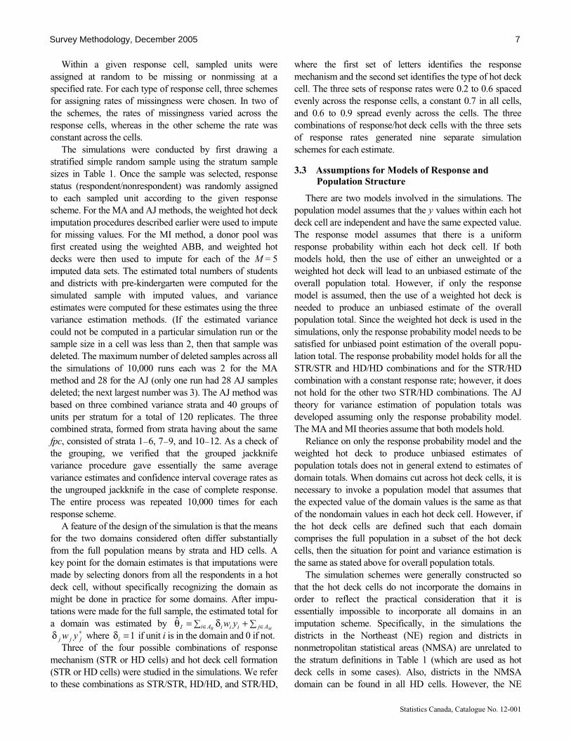
Figure 1 shows the results of the simulations for estimating the total number of students and the number of districts offering pre-kindergarten from the 10,000 samples for each of the nine simulation schemes. The figure gives the relative bias of the imputed estimator, the average variance estimate as a percentage of the empirical variance, and the confidence interval coverage rate.

Figure 1. Relative biases, variance ratios, and 95% confidence interval coverage for number of students (•) and number of districts with pre-kindergarten (∆).

Rel-bias (%) v/Var (%) 95% CI coverage

STR/STR 0.2 to 0.6 MA AJ MI

STR/STR 0.7 MA

AJ MI

STR/STR 0.6 to 0.9

MA AJ MI

HD/HD 0.2 to 0.6

MA AJ MI

HD/HD 0.7 MA

AJ MI

HD/HD 0.6 to 0.9 MA

AJ MI

STR/HD 0.2 to 0.6 MA

AJ MI

STR/HD 0.7 MA

AJ MI


AJ MI

-3.0 -2.0 -1.0 0.0 90 95 100 105 110 84 86 88 90 92 94 96 98



The point estimates are theoretically unbiased with weighted hot deck imputation if all units in a hot deck cell have the same response probability. As noted earlier, this condition holds for the STR/STR and HD/HD combinations and also for the STR/HD combination with a uniform overall response probability. The graph of relative biases in Figure 1 is consistent with this theoretical result within the bounds of simulation error. While the relative biases of the point estimates in the other two STR/HD schemes are small (always less than 3%), they still may be important if the standard errors of the estimates are also small. Cochran (1977, page 12) shows that when the ratio of the bias to the standard error is relatively large, then the coverage rate can be much lower than the nominal level. For the full population estimates with this sample size the ratios never exceed 0.4, but much larger ratios occur for domain estimates, as discussed later.

The graph of the ratios of the average variance estimates to the empirical variances (v/Var in the figures) for the three methods shows that these estimates have relatively small biases in most cases, within a range of plus or minus 8 percent around the simulated true variance. While the ratios for all the methods vary across the nine schemes, the MI ratios are slightly more variable than the other two.

A primary reason for computing variances is to produce confidence intervals. The right-hand panel in Figure 1 shows that the coverage rates for the confidence intervals for the estimates are generally close to the nominal 95 percent level, especially for the pre-kindergarten statistic. The coverage rates for both statistics and all the methods and schemes are between 91% and 96%, with the exception of the number of students for the STR/HD 0.2 to 0.6 scheme. The coverage rates of 88% or less for all three methods in this case, with its extremely high rate of nonresponse, are due to the relatively large bias in the point estimate. Overall, all three variance estimation methods produce confidence intervals with coverages that are vast improvements over those for intervals based on naïve variance estimates (Brick et al. 2004).

The confidence interval coverage rates for the MA and AJ methods are essentially equivalent. The MI coverage rates are generally slightly greater than those for the MA and AJ methods. The MI coverage rates are slightly closer to the nominal level for the number of students. Most of the differences are small.

For all three variance estimation methods, the upper and lower confidence interval coverage rates were similar. For the number of students, which is a highly skewed variable, the coverage rates in the two tails are unequal due to correlation between the estimated total and the standard error estimates. The asymmetric tail coverages are also associated with lower overall coverage rates.

The MA and AJ methods yield confidence intervals that have nearly the same average length across the schemes and variables. Because the MI method uses t – distribution values, its intervals range from 10 to 20 percent longer than the MA and AJ intervals when the response rates are low. With the higher response rates, the MI intervals range from about the same to 5 percent longer than the intervals from the two other methods. The MI confidence intervals could, of course, be shortened by increasing M (Rubin 1987, Chapter 4), even though M = 5 is typical for applications. 4.2 Domain Estimates

Estimating characteristics for domains that are not explicitly incorporated in the imputation scheme can be problematic when the missing data rate is not trivial. Kalton and Kaspryzk (1986) and Rubin (1996) along with many others have discussed this point and urged the inclusion of as many variables as possible in the imputation process. However, given the many preplanned and ad hoc domain analyses that are carried out with survey data, it is unrealistic to assume that all domains can be accounted for in an imputation scheme. For this reason, the design of the simulations intentionally did not include the domains explicitly in the definition of the hot deck cells. In the case of multiple imputation, issues of variance estimation for domain estimates have received much attention (e.g., Fay 1992; Meng 1994; Rubin 1996).

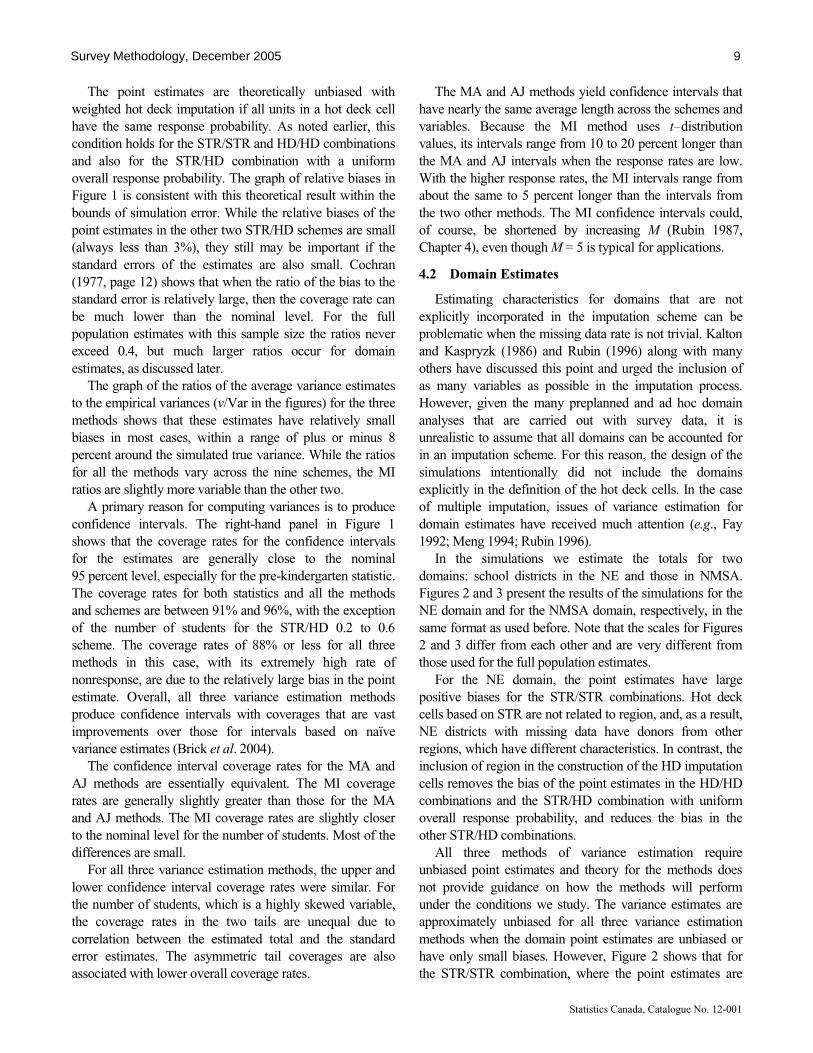
In the simulations we estimate the totals for two domains: school districts in the NE and those in NMSA. Figures 2 and 3 present the results of the simulations for the NE domain and for the NMSA domain, respectively, in the same format as used before. Note that the scales for Figures 2 and 3 differ from each other and are very different from those used for the full population estimates.

For the NE domain, the point estimates have large positive biases for the STR/STR combinations. Hot deck cells based on STR are not related to region, and, as a result, NE districts with missing data have donors from other regions, which have different characteristics. In contrast, the inclusion of region in the construction of the HD imputation cells removes the bias of the point estimates in the HD/HD combinations and the STR/HD combination with uniform overall response probability, and reduces the bias in the other STR/HD combinations.

All three methods of variance estimation require unbiased point estimates and theory for the methods does not provide guidance on how the methods will perform under the conditions we study. The variance estimates are approximately unbiased for all three variance estimation methods when the domain point estimates are unbiased or have only small biases. However, Figure 2 shows that for the STR/STR combination, where the point estimates are



seriously biased, the variance estimates usually overestimate the empirical variances.

Figure 2 shows that the coverage rates for the HD/HD and STR/HD schemes – for which the point estimates have no or small relative biases – are between 92 percent and 96 percent for all but one of these schemes and variance estimation methods. The exception is the STR/HD combination with response rates between 0.2 and 0.6, which has coverage rates as low as 86 percent for the number of students.

For the STR/STR schemes, Figure 2 shows that all the methods tend to cover at greater than the nominal level for the number of students and less than the nominal level for the number of districts with pre-kindergarten. The difference in the coverage rates for the two variables is due to the sizes of the relative bias of the point estimates and of the variance estimates.

Turning to the NMSA domain estimates in Figure 3, note that metropolitan status is not explicitly included in the

definitions of either STR or HD, although it is clearly correlated with size and, thus, with STR. The point estimates for the number of students in the NMSA domain for all the schemes have substantial positive biases. The MA confidence intervals consistently cover at the nominal level or higher, primarily due to the extreme positive biases of the variance estimates. The AJ intervals cover at close to the nominal level for the HD/HD and STR/HD schemes, but undercover in the three STR/STR schemes. The patterns for the MI coverages are similar to those of the AJ, except that the MI intervals appreciably undercover in the HD/HD scheme with 0.2 to 0.6 response rates.

The point estimates of the number of districts with pre-kindergarten in the NMSA domain have moderate negative relative biases for all nine schemes. The confidence intervals for all three methods of variance estimation are close to the nominal level, without the overcoverage found in the NE domain estimates.

Figure 2. Relative biases, variance ratios, and 95% confidence interval coverage for number of students (•) and number of districts with pre-kindergarten (∆) in the Northeast.


STR/STR 0.2 to 0.6 MA

AJ MI

STR/STR 0.7 MA

AJ MI

STR/STR 0.6 to 0.9

MA AJ MI

HD/HD 0.2 to 0.6

MA AJ MI

HD/HD 0.7 MA

AJ MI

HD/HD 0.6 to 0.9 MA

AJ MI


AJ MI

STR/HD 0.7 MA

AJ MI


AJ MI



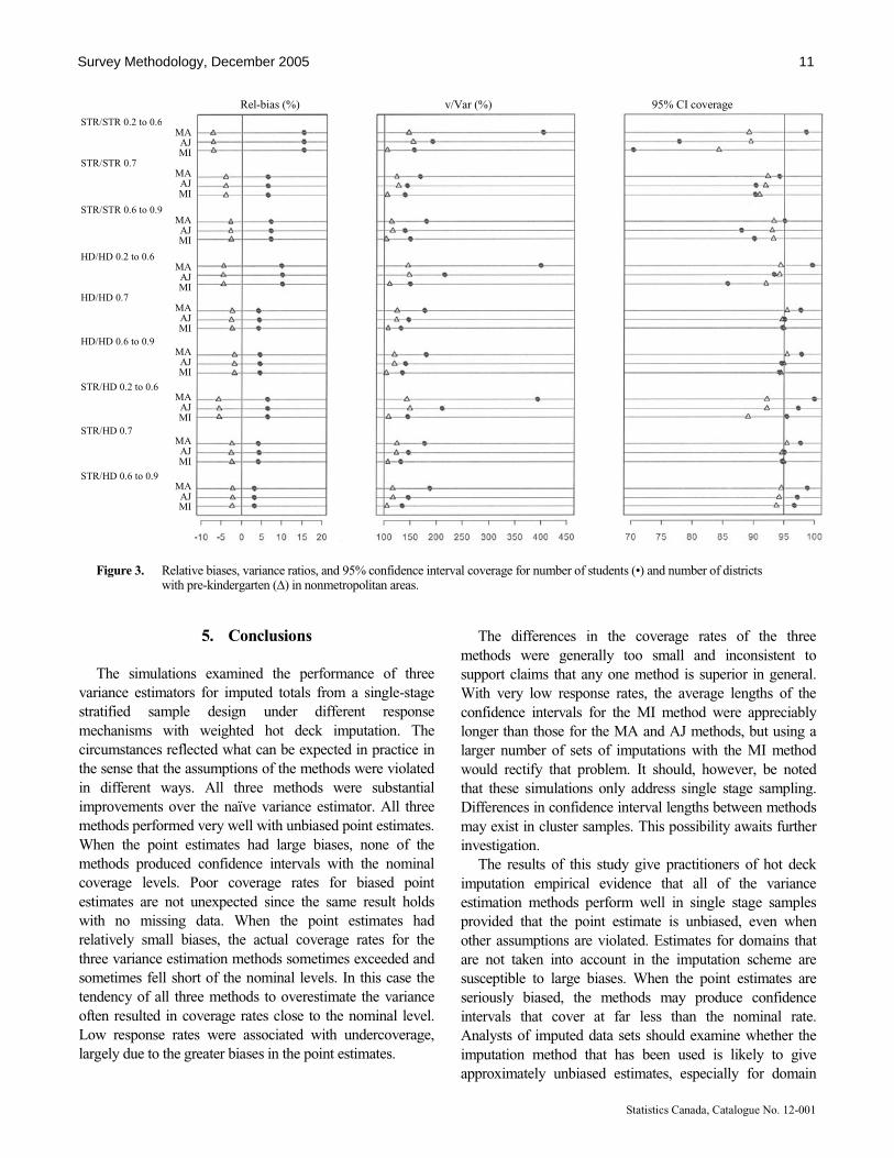
Figure 3. Relative biases, variance ratios, and 95% confidence interval coverage for number of students (•) and number of districts with pre-kindergarten (∆) in nonmetropolitan areas.

5. Conclusions The simulations examined the performance of three

variance estimators for imputed totals from a single-stage stratified sample design under different response mechanisms with weighted hot deck imputation. The circumstances reflected what can be expected in practice in the sense that the assumptions of the methods were violated in different ways. All three methods were substantial improvements over the naïve variance estimator. All three methods performed very well with unbiased point estimates. When the point estimates had large biases, none of the methods produced confidence intervals with the nominal coverage levels. Poor coverage rates for biased point estimates are not unexpected since the same result holds with no missing data. When the point estimates had relatively small biases, the actual coverage rates for the three variance estimation methods sometimes exceeded and sometimes fell short of the nominal levels. In this case the tendency of all three methods to overestimate the variance often resulted in coverage rates close to the nominal level. Low response rates were associated with undercoverage, largely due to the greater biases in the point estimates.

The differences in the coverage rates of the three methods were generally too small and inconsistent to support claims that any one method is superior in general. With very low response rates, the average lengths of the confidence intervals for the MI method were appreciably longer than those for the MA and AJ methods, but using a larger number of sets of imputations with the MI method would rectify that problem. It should, however, be noted that these simulations only address single stage sampling. Differences in confidence interval lengths between methods may exist in cluster samples. This possibility awaits further investigation.

The results of this study give practitioners of hot deck imputation empirical evidence that all of the variance estimation methods perform well in single stage samples provided that the point estimate is unbiased, even when other assumptions are violated. Estimates for domains that are not taken into account in the imputation scheme are susceptible to large biases. When the point estimates are seriously biased, the methods may produce confidence intervals that cover at far less than the nominal rate. Analysts of imputed data sets should examine whether the imputation method that has been used is likely to give approximately unbiased estimates, especially for domain


STR/STR 0.2 to 0.6 MA AJ MI

STR/STR 0.7 MA AJ MI

STR/STR 0.6 to 0.9

MA AJ MI

HD/HD 0.2 to 0.6

MA AJ MI

HD/HD 0.7 MA AJ MI

HD/HD 0.6 to 0.9 MA AJ MI

STR/HD 0.2 to 0.6 MA AJ MI

STR/HD 0.7 MA AJ MI

STR/HD 0.6 to 0.9 MA AJ MI



estimates. If not, they may need to re-impute the missing items to give less biased point estimates. Advice to imputers to take advantage of as many explanatory variables as feasible in the imputation process is not new, but the evidence from the simulations demonstrates its importance.

Acknowledgements

The authors would like to thank the National Center for Education Statistics, Institute for Education Sciences for supporting this research, and in particular Marilyn Seastrom. We also would like to thank the referees for their constructive comments.

References

Brick, J.M., Kalton, G. and Kim, J.K. (2004). Variance estimation with hot deck imputation using a model. Survey Methodology, 30, 57-66.

Brick, J.M., Jones, M., Kalton, G. and Valliant, R. (2004). A simulation study of three methods of variance estimation with hot deck imputation for stratified samples. Prepared under contract No. RN95127001 to the National Center for Education Statistics. Rockville, MD: Westat, Inc.

Cochran, W.G. (1977). Sampling Techniques. New York: John Wiley & Sons Inc.

Fay, R.E. (1992). When are imputations from multiple imputation valid. Proceedings of the Survey Research Methods Section, American Statistical Association, 227-232.

Kalton, G., and Kasprzyk, D. (1986). The treatment of missing survey data. Survey Methodology, 12, 1-16.

Lee, H., Rancourt, E. and Särndal, C.-E. (1995). Jackknife variance estimation for data with imputed values. Proceedings of the Statistical Society of Canada Survey Methods Section, 111-115.

Lee, H., Rancourt, E. and Särndal, C.-E. (2001). Variance estimation from survey data under single imputation. In Survey Nonresponse (Eds. R.M. Groves, D.A. Dillman, J.L. Eltinge and R.J.A Little), Chapter 21, New York: John Wiley & Sons Inc.

Little, R.J.A., and Rubin, D.B. (2002). Statistical Analysis with Missing Data. New York: John Wiley & Sons Inc.

Meng, X.-L. (1994). Multiple imputation inferences with uncongenial sources of input. (With discussion). Statistical Science, 9, 538-573.

Rao, J.N.K., and Shao, J. (1992). Jackknife variance estimation with survey data under hot deck imputation. Biometrika, 79, 811-822.

Rubin, D.B. (1987). Multiple Imputation for Nonresponse in Surveys. New York: John Wiley & Sons Inc.

Rubin, D.B. (1996). Multiple imputation after 18+ years (with discussion). Journal of the American Statistical Association, 91, 473-489.

Rubin, D.B., and Schenker, N. (1986). Multiple imputation for interval estimation from simple random samples with nonignorable nonresponse. Journal of the American Statistical Association, 81, 361-374.

Rust, K., and Rao, J.N.K. (1996). Variance estimation for complex estimators in sample surveys. Statistics in Medicine, 5, 381-397.

Särndal, C.-E. (1992). Methods for estimating the precision of survey estimates when imputation has been used. Survey Methodology, 18, 241-252.

Shao, J., and Steel, P. (1999). Variance estimation for survey data with composite estimation and nonnegligible sampling fractions. Journal of the American Statistical Association, 94, 254-265.


Documents

Variance Estimation with Hot Deck Imputation: A Simulation ... · PDF fileknife method (Rao and Shao 1992), and multiple imputation (Rubin 1987). Each method has been evaluated theoretically