Embed Size (px)
Citation preview

Multiple Imputation of Right-Censored Wages in the
German IAB Employment Register Considering
Heteroscedasticity
Thomas Buttner and Susanne Rassler
Institute for Employment Research of the German Federal Employment Agency,
Research Unit for Statistical Methods
Regensburger Straße 104, 90478 Nuremberg
email: [email protected], [email protected]
SUMMARY: In many large data sets of economic interest, some variables, as wages, are top-coded or right-
censored. In order to analyze wages with the German IAB-employment register we first have to solve the
problem of censored wages at the upper limit of the social security system. We treat this problem as a
missing data problem and use multiple imputation approaches to impute the censored wages by draws of a
random variable from a truncated distribution, based on Markov chain Monte Carlo techniques. In general,
the dispersion of income is smaller in lower wage categories than in higher categories and the assumption
of homoscedasticity in an imputation model is highly questionable. Therefore, we suggest a new multiple
imputation method which does not presume homoscedasticity of the residuals. Finally, in a simulation
study, different imputation approaches are compared under different situations and the necessity as well as
the validity of the new approach is confirmed.
Key words: multiple imputation, missing data, censored wage data, simulation study

Contents
1 Introduction 3
2 Imputation approaches for censored wages 4
2.1 Homoscedastic imputation approaches . . . . . . . . . . . . . . . . . . . . 5
2.1.1 Homoscedastic single imputation . . . . . . . . . . . . . . . . . . . 5
2.1.2 Multiple imputation . . . . . . . . . . . . . . . . . . . . . . . . . . 6
2.2 Heteroscedastic imputation approaches . . . . . . . . . . . . . . . . . . . . 8
2.2.1 Heteroscedastic single imputation . . . . . . . . . . . . . . . . . . . 8
2.2.2 Multiple imputation considering heteroscedasticity . . . . . . . . . . 8
3 Simulation study 10
3.1 The IAB employment register . . . . . . . . . . . . . . . . . . . . . . . . . 10
3.2 Creating a complete population . . . . . . . . . . . . . . . . . . . . . . . . 11
3.3 Simulation design . . . . . . . . . . . . . . . . . . . . . . . . . . . . . . . 12
4 Results 15
4.1 Homoscedastic data set . . . . . . . . . . . . . . . . . . . . . . . . . . . . . 15
4.2 Heteroscedastic data set . . . . . . . . . . . . . . . . . . . . . . . . . . . . 17
5 Conclusion 19
6 References 20
2

1 Introduction
For a large number of research questions, like analyzing the gender wage gap or measuring
overeducation with earnings frontiers, it is interesting to analyze income data. To address
this kind of questions two types of data are used: surveys and process generated data.
Process generated data have several advantages, like a large number of observations, no
nonresponse burden and no problems with interviewer effects or survey bias. Unfortu-
nately, in many large process generated data sets of economic interest some variables,
such as wages, are top-coded or right-censored. This problem is very common with ad-
ministrative data from social security systems like the IAB employment register (IABS),
which is edited from the data of the German unemployment insurance. The contribution
rate of this insurance is charged percentaged from the gross wage. Is the gross wage
higher than the current contribution limit, however only the amount of the limit is liable
for the contribution. In 2007 the contribution limit in the unemployment insurance is
fixed at a monthly income of 5,250 euros. As therefore wages are only recorded up to this
contribution limit, the income information in this register is censored at this limit.
In order to analyze wages with this register, we first have to solve the problem of the
censored wages. We treat this problem as a missing data problem and use imputation
approaches to impute the censored wages. Gartner (2005) proposes a single imputation
approach to solve the problem of the censored wages. A further approach - a multiple
imputation method based on draws of a random variable from a truncated distribution
and Markov Chain Monte Carlo techniques - is suggested by Gartner and Rassler (2005).
These two approaches presume homoscedasticity of the residuals, but since in general,
the dispersion of income is smaller in lower wage categories than in higher categories, the
assumption of homoscedasticity in an imputation model is highly questionable. Therefore
we use a third approach, a second single imputation approach based on GLS estimation
to consider heteroscedasticity.
A first simulation study using these three methods shows the necessity to develop a new
method that imputes the missing wage information multiple and does not presume ho-
moscedasticity. Therefore we suggest a new multiple imputation method and finally com-
pare in a simulation study the four different imputation approaches again under different
3

0.5
11.
52
2.5
Den
sity
3 4 5 6ln(wage)
Distribution of wages in the IABS
Figure 1: Distribution of wages in logs in the IAB employment register
situations in order to confirm the necessity as well as the validity of the new approach.
2 Imputation approaches for censored wages
Before we develop and evaluate a new approach, the first section of this paper describes
the three different approaches, which were already proposed to impute the missing wage
information in the IAB employment register. All of them assume that the wage in logs y
for every person i is given by
yi∗ = xiβ + εi where ε ∼ N(0, σ2). (1)
As the wages in the IAB employment register are censored at the contribution limit a we
observe the wage yobs = y∗i only if the wage is lower than the treshold a. If the wage is
censored, we observe the limit a instead of the true wage y∗i :
yi =
yobs if yi ≤ a
a if yi > a(2)
To be able to analyze wages with our data set, we first have to impute the wages above
a. Thus we define y = (yobs, a) and yz = (yobs,z). So z is a truncated variable in the
4

range (a,∞). We regard the missingness mechanism as not missing at random (NMAR,
according to Little and Rubin, 1987, 2002) as well as missing by design. The first because
the missingness depends on the value itself. If the limit is exceeded the true value will
not be reported but the value of the limit a. The latter because the data are missing due
to the fact that they were not asked.
2.1 Homoscedastic imputation approaches
2.1.1 Homoscedastic single imputation
One possibility to impute the missing wage information is using a single imputation ap-
proach. A homoscedastic single imputation (without consideration of heteroscedasticity)
can be performed based on a tobit model. The tobit model is used to estimate the pa-
rameter β of the imputation model. According to the estimated parameters the censored
wage z can be imputed by draws of a random value. As we know that the true value is
above the contribution limit we have to draw a random variable from a truncated normal
distribution
z∗i ∼ Ntrunca(x′β, σ2). (3)
This means we add to the expected wage an error term ε with the standard deviation σ
(estimated from the tobit estimation):1
z∗i = x′β + ε (4)
Using a single imputation approach, we have to consider that this method may lead
to biased variance estimations. Thus Little and Rubin (1987) suggest that imputation
should rather be done in a multiple and bayesian way. Therefore we better use multiple
imputation approaches to impute the missing wage information.
1For more information on this approach see Gartner (2005).
5

2.1.2 Multiple imputation
To start with, let Y = (Yobs, Ymis) denote the random variables concerning the data with
observed and missing parts. In our specific situation this means that for all units with
wages below the limit a each data record is complete, i.e., Y = (Yobs) = (X, wages). For
every unit with a value of the limit a for its wage information we treat the data record
as partly missing, i.e., Y = (Yobs, Ymis) = (X, ?). Thus, we have to multiply impute the
missing data Ymis = wage. The theory and principle of multiple imputation originates
from Rubin (1978) and is based on independent random draws from the posterior predic-
tive distribution fYmis|Yobsof the missing data given the observed data. As is it may be
difficult to draw from fYmis|Yobsdirectly, a two-step procedure for each of the m draws is
useful:
1. First, we perform random draws of the parameter Ξ according to their observed-data
posterior distribution fΞ|Yobs,
2. Then, we make random draws of Ymis according to their conditional predictive
distribution fYmis|Yobs,Ξ.
Because
fYmis|Yobs(ymis|yobs) =
∫fYmis|Yobs,Ξ(ymis|yobs,ξ)fΞ|Yobs
(ξ|yobs)dξ (5)
holds, with (1) and (2) we achieve imputations of Ymis from their posterior predictive
distribution fYmis|Yobs. Due to the data generating model used, for many models the
conditional predictive distribution fYmis|Yobs,Ξ is rather straightforward. That means it
can be easily formulated for each unit with missing data. In contrast, the corresponding
observed-data posteriors fΞ|Yobsare usually difficult to derive for those units with missing
data, especially when the data have a multivariate structure. The observed data
posteriors are often no standard distributions from which random numbers can easily be
generated. However, simpler methods have been developed to enable multiple imputation
based on Markov chain Monte Carlo (MCMC) techniques (Schafer 1997). In MCMC
the desired distributions fYmis|Yobsand fΞ|Yobs
are achieved as stationary distributions of
6

Markov chains based on the complete-data distributions, which is easier to compute. 2
Imputation model
To be able to start the imputation based on MCMC, we first need to adapt starting values
for β(0) and the variance σ2(0) ( for programming reasons below defined as τ−2(0)) from a
ML tobit estimation. Second, in the imputation step, we randomly draw values for the
missing wages from the truncated distribution analog to the single imputation procedure
z∗(t)i ∼ Ntrunca(x
′β(t), τ−2(t)). (6)
Then a OLS regression is computed based on the imputed data sets according to
βz(t) = (X ′X)−1X ′y(t)z (7)
After this, we can produce new random draws for the parameters according to their
complete data posterior distribution. Since drawings from a gamma distribution are
complicated to compute with STATA, we draw the variance in the posterior step as
follows:
g ∼ χ2(n− k) (8)
τ 2(t+1) =g
RSS(9)
where RSS is the residual sum of squares RSS =n∑
t=1
(yz(t)i− x′iβ
(t)z )2 and k is the number
of columns of X.
Now we perform new random draws for the parameters β
βt+1 ∼ N(β(t)z , τ−2(t+1)(X ′X)−1) (10)
2For more details see Gartner and Rassler (2005)
7

We repeat the imputation and the posterior-step 5,000 times and use
(z2000i , z3000
i , . . . , z11000i ) to obtain 5 complete data sets. 3
2.2 Heteroscedastic imputation approaches
2.2.1 Heteroscedastic single imputation
As we assume the dispersion of income to be smaller in lower wage categories than in
higher categories, we suppose the necessity of an approach considering heteroscedasticity.
Therefore we develop another single imputation procedure based on the first single impu-
tation approach, a method that does not presume homoscedasticity of the residuals. We
develop this method in order to check wether we need to do further research towards a
multiple imputation approach considering heteroscedasticity.
Here we use a GLS model for truncated variables to estimate the parameters of the
imputation model, the coefficients β, like in the first approach, and furthermore the
parameters γ, describing the heteroscedasticity. Then the imputation can be done by
draws from a truncated normal distribution, similar to the first approach,
z∗i ∼ Ntrunca(x′β, σ2
i ) where σ2i = em′γ. (11)
To consider the heteroscedastic structure of the residuals, we use here individual variances
for every person. This procedure is a solution that takes into consideration the existence
of heteroscedasticity, yet it does not solve the problem of biased variance estimations.
2.2.2 Multiple imputation considering heteroscedasticity
Since we assume the necessity of an approach that does not presume homoscedasticity
and since Little and Rubin show that single imputation approaches may lead to biased
variance estimations, consequently we suggest an approach that multiply imputes the
missing wage information and considers heteroscedasticity of the residuals. A first simula-
tion study using the first three approaches shows as well the need for this approach. This
simulation study points out that, in case of a homoscedastic structure of the residuals,
3For further details on this approach see Gartner and Rassler (2005).
8

the multiple imputation leads to better results than a single imputation approach.
But in case of heteroscedasticity the single imputation considering heteroscedasticity is
superior to the multiple imputation approach suggested by Gartner and Rassler. This
indicates the necessity to develop another approach that combines these two properties:
an approach performing multiple imputation and considering heteroscedasticity.
Imputation model
We develop this new method based on the multiple imputation approach proposed by
Gartner and Rassler (2005). The basic element of the new approach is that we need
additional draws for the parameters γ describing the heteroscedasticity. We start now
the imputation by adapting starting values for β(0), γ(0)and τ−2(0) from a GLS estimation
for truncated variables. Then we are able to draw values for the missing wages from
a truncated distribution using individual variances σi = ex′γ like in the heteroscedastic
single imputation model:
z∗(t)i ∼ Ntrunca(x
′β(t), σ2(t)i ) where σ
2(t)i = em′γ. (12)
Then a GLS regression is computed based on the imputed data set (comparable to the
OLS regression in the heteroscedastic multiple imputation approach). Afterwards we pro-
duce new random draws for the parameters according to their complete data posterior
distribution. As we consider now the existence of heteroscedasticity, some slight modi-
fications to the algorithm are necessary. In the first step, we draw the variance τ 2(t+1)
according to
g ∼ χ2(n− k) (13)
τ 2(t+1) =g
RSSwhere RSS =
n∑t=1
exp(ln εi −m′iγ) =
n∑t=1
(y(t)i − x′iβ
(t)i )2
em′γ (14)
In a additional step, we have to perform random draws for γ
9
γt+1 ∼ N(γ(t)z , τ−2(t)
γ (M ′M)−1) (15)
Consequently the parameters β can be drawn like in the Gartner and Rassler approach,
again with a slight modification compared to the homoscedastic multiple imputation:
βt+1|γt+1, τ 2(t+1) ∼ N(β(t)z , τ−2(t+1)(
n∑t=1
X ′Xem′γ )−1) (16)
We repeat these steps again 5,000 times and use (z2000i , z3000
i , . . . , z11000i ) to obtain the 5
complete data sets.
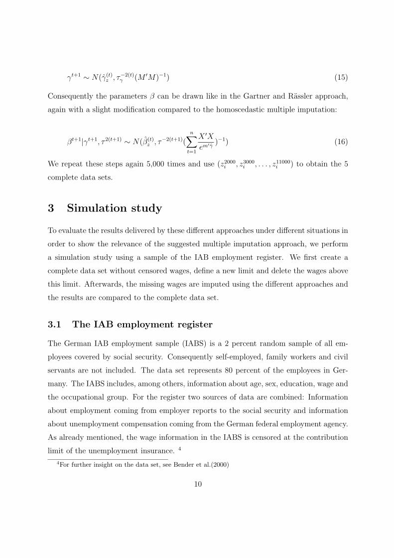
3 Simulation study
To evaluate the results delivered by these different approaches under different situations in
order to show the relevance of the suggested multiple imputation approach, we perform
a simulation study using a sample of the IAB employment register. We first create a
complete data set without censored wages, define a new limit and delete the wages above
this limit. Afterwards, the missing wages are imputed using the different approaches and
the results are compared to the complete data set.
3.1 The IAB employment register
The German IAB employment sample (IABS) is a 2 percent random sample of all em-
ployees covered by social security. Consequently self-employed, family workers and civil
servants are not included. The data set represents 80 percent of the employees in Ger-
many. The IABS includes, among others, information about age, sex, education, wage and
the occupational group. For the register two sources of data are combined: Information
about employment coming from employer reports to the social security and information
about unemployment compensation coming from the German federal employment agency.
As already mentioned, the wage information in the IABS is censored at the contribution
limit of the unemployment insurance. 4
4For further insight on the data set, see Bender et al.(2000)
10

To simplify the simulation design, we restrict the data for the simulation to male West-
German residents. We use all workers holding a full-time job covered by social security
effective on June 30th 2000. The data set contains 214,533 persons: 23,685 or 11 percent
of them with censored wages. The following table shows descriptive information about the
fraction of censored incomes of 6 educational and 5 age groups to demonstrate the need
to impute the missing wage information. Especially for analyzing highly-skilled workers
the table indicates the necessity to impute the missing wages.
<25 25-34 35-44 45-54 55+
educ1 0 .003 .008 .012 .17
educ2 .001 .021 .068 .116 .150
educ3 .010 .110 .232 .331 .371
educ4 .003 .110 .283 .393 .470
educ5 .024 .190 .450 .558 .604
educ6 .056 .256 .549 .686 .769
Table 1: Censored wages in the original data set
For the simulation study we assume a model containing the wage in logs as dependent
variable and age, squared age, nationality as well as six dummies for education levels and
four categories of job level as independent variables.
3.2 Creating a complete population
To perform the simulation study, a complete population is needed in to order to be
able to compare the results of the different approaches with a complete data base. As
the IABS employment register is right-censored, we first have to impute our sample to
obtain this control population. The fact that the data set has to be imputed before
starting the simulation study allows us to produce control populations with different
characteristics: We create one data set where homoscedasticity is existent and another
with heteroscedasticity of the residuals. To obtain the first data set (Data set A) we use
the homoscedastic single imputation procedure as described in section 2.1.1 to impute new
11

wages for every person regardless if the wage was originally censored or not, according to
ynew ∼ Ntrunca(x′β, σ2). (17)
A test for heteroscedasticity shows constant variances for this data set. To receive the
second data set (Data set B), the heteroscedastic single imputation method described in
section 2.2.1 is used in order to get a control population with heteroscedasticity of the
residuals, according to
ynew ∼ Ntrunca(x′β, em′γ). (18)
A test for heteroscedasticity shows no constant variances, which refers to heteroscedas-
ticity of the residuals in this data set. This two data sets will later be used as complete
populations for the analysis of the results we receive by using the different approaches.
3.3 Simulation design
The simulation study consists of four steps. Each of these steps is simultaneously done
for the homoscedastic data set A and the heteroscedastic population B: We draw random
samples from the complete population repeatedly, define a new threshold and impute the
wage above this threshold using the four approaches. Then we compare the imputed data
sets with the complete population. To clarify the proceeding we describe the procedure
only for one of the two options.
Step 1: Drawing of a random sample
In the first step a random sample of n=21,453 persons is drawn without replacement
from the population of N=214,533 persons (equivalent to 10 percent). This 10 percent
random sample is kept to illustrate the results of the different imputations later. For the
simulation study we define a new threshold. To point out the differences between the
four approaches we choose a limit lower than in the original IABS (censoring the highest
30 percent of incomes appears adequate) and delete the incomes above this limit.
12

Step 2: Imputation of the missing wage information
The deleted wage information above the threshold of this (now right-censored) sample is
imputed by using the four different approaches described above:
• Homoscedastic single imputation
• Heteroscedastic single imputation
• Multiple imputation
• Multiple imputation considering heteroscedasticity
That means by each of the single imputation methods, one complete data set is obtained
and by each of the multiple imputation methods, five complete data sets. This imputed
data sets now can be used to evaluate the quality of the different approaches by comparing
them with the original complete population.
Step 3: Analysis of the results
To analyze the results of the imputations we run OLS regressions on the imputed data sets
and the 10 percent complete random sample on the one side, on the complete population
on the other side. We use as estimation model - simulating an analysis which is typically
done with income data - the same model as the imputation model. Afterwards we can
evaluate which approach delivers the best imputation quality compared to the original
complete data. Therefore we compare the parameter β - estimated based on the imputed
data sets - with the results β of the regression on the complete population.
For this purpose we need to use the parameter β as well as the corresponding confidence
intervals. Since the multiple imputation approaches lead to five complete data sets, the
estimations have to be done five times as well and afterwards, the results have to be
combined following Rubin (1987) in order to get valid parameters and confidence inter-
vals. Thus, the multiple imputation point estimate for β is the average of the five point
estimates
β =1
m
m∑t=1
β(t). (19)
13

The variance estimate associated with β has two components. The within-imputation-
variance is the average of the complete-data variance estimates,
U =1
m
m∑t=1
U (t). (20)
The between-imputation variance is the variance of the complete-data point estimates
B =1
m− 1
m∑t=1
(β(t) − β)2. (21)
Subsequently the total variance is defined as
T = U + (1 + m−1)B. (22)
For large sample sizes, tests and two-sided (1− α) ∗ 100% interval estimates for multiply
imputed data sets can be calculated based on the Student‘s t-distribution
(β − β)/√
T ∼ tv and β ± tv,1−α/2
√T (23)
with the degrees of freedom
v = (m− 1)(1 +U
(1 + m−1)B)2. (24)
We save for every approach in every iteration the parameter β and the corresponding
standard error of β, as well as the 95 percent confidence interval of β. Besides, we keep the
information if the confidence interval of β contains the parameter β of the original data set.
Step 4: 1000 iterations
The whole simulation procedure - consisting of drawing a random sample, imputing the
data using the different approaches, running a regression on the different imputed data
sets and calculating the confidence intervals - is repeated 1000 times. Finally the fraction
of confidence intervals of β containing the true parameter β can be calculated for the
different approaches. The results of this iterations are described in the following chapter.
14

4 Results
This chapter contains tables showing the results of the simulation study comparing the
four different approaches. The first column contains the true parameter β, estimated using
the original complete population. The following columns show the parameter β (here the
average of the 1000 iterations) of the regression using the 10 percent complete random
samples and the regressions using the data sets imputed by the different approaches. The
tables show as well the fraction of iterations where the 95 percent confidence interval of
β contains the parameter β (coverage).
4.1 Homoscedastic data set
The first table shows the results of the simulation based on the homoscedastic data set A.
As expected, the simulation study shows the necessity of a multiple imputation approach,
since the coverage of the two multiple imputation approaches is higher than of the single
imputations throughout almost all variables. Using a homoscedastic data set, the results
do not show serious differences between the homoscedastic and the heteroscedastic mul-
tiple imputation. We receive a coverage for both of this approaches around 95 percent
(between 0.965 and 0.922) - similar to the coverage received by the estimations using the
complete random samples (between 0.965 and 0.948) - which refers to a good imputation
quality. The coverage of the single imputations, especially the single imputation consid-
ering heteroscedasticity, is for most of the variables lower than 0.95. Consequently, it can
be concluded, that in case of a homoscedastic structure of the residuals, it is advisable
to use a multiple imputation approach. However it does not matter if the algorithm con-
sidering heteroscedasticity is chosen in the homoscedastic case, since it just represents a
generalization of the homoscedastic approach and therefore works just as well in case of
homoscedasticity.
15

com
ple
tedat
asi
ngl
ehom
osc.
singl
ehet
eros
c.m
ult
iple
hom
osc.
mult
iple
het
eros
c.
ββ
Cov
erag
eβ
Cov
erag
eβ
Cov
erag
eβ
Cov
erag
eβ
Cov
erag
e
educ1
0.10
680.
1069
0.95
90.
1074
0.95
10.
1073
0.95
0.10
740.
958
0.10
730.
958
educ2
0.17
910.
1790
0.96
50.
1792
0.95
30.
1790
0.95
20.
1792
0.96
50.
1790
0.96
1
educ3
0.13
050.
1310
0.95
40.
1317
0.93
90.
1330
0.93
50.
1318
0.95
50.
1330
0.95
7
educ4
0.26
210.
2623
0.96
30.
2624
0.92
80.
2654
0.88
80.
2624
0.95
70.
2653
0.94
9
educ5
0.44
450.
4446
0.94
80.
4409
0.86
80.
4466
0.75
90.
4410
0.94
40.
4469
0.92
2
educ6
0.50
980.
5096
0.96
20.
5064
0.85
20.
5121
0.71
90.
5065
0.95
30.
5118
0.92
9
leve
l10.
5449
0.54
410.
949
0.54
400.
952
0.54
470.
950.
5440
0.94
90.
5446
0.95
leve
l20.
6517
0.65
120.
950.
6515
0.95
40.
6524
0.95
10.
6515
0.95
20.
6523
0.95
1
leve
l30.
8958
0.89
500.
948
0.89
730.
950.
8958
0.93
60.
8976
0.94
80.
8959
0.95
4
leve
l40.
8962
0.89
560.
953
0.89
610.
950.
8962
0.94
90.
8962
0.95
10.
8963
0.95
1
age
0.04
980.
0498
0.95
50.
0500
0.94
30.
0500
0.93
0.05
000.
964
0.05
000.
957
sqag
e-0
.000
5-0
.000
50.
958
-0.0
005
0.93
6-0
.000
50.
922
-0.0
005
0.96
2-0
.000
50.
96
nat
ion
-0.0
329
-0.0
327
0.96
2-0
.033
40.
948
-0.0
334
0.94
2-0
.033
50.
953
-0.0
334
0.95
5
cons
2.44
242.
4433
0.95
32.
4406
0.94
52.
4405
0.93
22.
4411
0.95
12.
4406
0.94
9
Tab
le2:
Res
ult
sof
the
hom
osce
das
tic
dat
ase
t
16

4.2 Heteroscedastic data set
The results based on the heteroscedastic data set B show a different situation. First the
results recommend as well the use of a multiple imputation approach, since the coverage
of the single imputation approaches is again lower than 0.95 for all variables. Concerning
the heteroscedastic structure of the residuals, it reveals the necessity of an approach
considering heteroscedasticity. The homoscedastic approaches deliver in several cases
a significant lower coverage than the procedures that consider heteroscedasticity. The
coverage of the heteroscedastic multiple imputation approach amounts again to around
95 percent and is similar to the coverage of the complete random samples (the coverage
ranges between 0.97 and 0.917, except the dummy for the highest education level where
the coverage is 0.896). In this case, the coverage of the conventional multiple imputation is
significant lower (between 0.948 and 0.478, for some variables even lower than the coverage
received by the heteroscedastic single imputation approach, where the coverage ranges
between 0.948 and 0.718). Therefore the results suggest the use of an approach considering
heteroscedasticity to impute the missing wage information in case of a heteroscedastic
structure of the residuals .
17

com
ple
tedat
asi
ngl
ehom
osc.
singl
ehet
eros
c.m
ult
iple
hom
osc.
mult
iple
het
eros
c.
ββ
Cov
erag
eβ
Cov
erag
eβ
Cov
erag
eβ
Cov
erag
eβ
Cov
erag
e
educ1
0.11
410.
1145
0.95
20.
1271
0.79
40.
1136
0.94
50.
1272
0.80
40.
1136
0.95
5
educ2
0.19
120.
1915
0.95
50.
2075
0.61
60.
1903
0.94
80.
2076
0.63
20.
1903
0.95
5
educ3
0.14
420.
1444
0.96
10.
0947
0.74
50.
1406
0.94
20.
0952
0.76
90.
1420
0.96
3
educ4
0.26
850.
2686
0.96
10.
2753
0.91
30.
2688
0.92
20.
2754
0.93
70.
2689
0.96
educ5
0.44
330.
4435
0.96
30.
4790
0.36
60.
4372
0.76
10.
4796
0.47
80.
4377
0.91
7
educ6
0.52
410.
5248
0.95
40.
5117
0.78
50.
5164
0.71
80.
5121
0.86
90.
5161
0.89
6
leve
l10.
5422
0.54
260.
955
0.54
150.
946
0.54
220.
947
0.54
160.
946
0.54
170.
953
leve
l20.
6405
0.64
110.
950.
6430
0.94
40.
6412
0.94
40.
6430
0.94
70.
6407
0.95
leve
l30.
8856
0.88
640.
945
0.87
800.
941
0.88
450.
945
0.87
820.
948
0.88
380.
952
leve
l40.
8903
0.89
080.
952
0.87
370.
941
0.89
190.
943
0.87
370.
941
0.89
130.
951
age
0.04
320.
0431
0.95
50.
0457
0.64
50.
0431
0.94
80.
0457
0.67
90.
0431
0.97
sqag
e-0
.000
4-0
.000
40.
96-0
.000
50.
59-0
.000
40.
941
-0.0
005
0.62
3-0
.000
40.
968
nat
ion
-0.0
223
-0.0
218
0.96
1-0
.029
70.
872
-0.0
222
0.94
5-0
.029
60.
882
-0.0
222
0.95
4
cons
2.58
582.
5865
0.94
72.
5318
0.90
92.
5868
0.94
52.
5315
0.91
42.
5875
0.95
2
Tab
le3:
Res
ult
sof
the
het
eros
cedas
tic
dat
ase
t
18

5 Conclusion
There is a diversity of ways to deal with censored wage data. We propose to use imputa-
tion approaches to estimate the missing wage information and to so solve this problem.
Nevertheless, there are also different possibilities to impute the wages in the IABS, for ex-
ample single and multiple imputation approaches. Another important question is wether
the wages should be imputed considering heteroscedasticity or not.
In this paper we propose a new approach to multiply impute the missing wage infor-
mation above the limit of the social security in the IAB employment register. We have
assumed the dispersion of income to be smaller in lower wage categories than in higher
categories. Thus we have suggested and developed a multiple imputation approach con-
sidering heteroscedasticity to impute the missing wage information. The basic element
of this approach is to impute the missing wages by draws of a random variable from a
truncated distribution, based on Markov chain Monte Carlo techniques. The main in-
novation of the suggested approach is to perform additional draws for the parameter γ
describing the heteroscedasticity in order to be able to allow individual variances for ev-
ery individuum. To confirm the necessity and validity of this new method we have used
a simulation study to compare the different approaches. The results of the simulation
study can be subsumed as follows: The missing wage information should be imputed
rather multiple. This is due to two reasons: First, because single imputations may lead to
biased variance estimations and second (as the simulation study shows), because multiple
imputation approaches lead to better imputation results. Furthermore, the imputation
should be done considering heteroscedasticity. In case of homoscedastic residuals the same
quality of imputation results can be expected compared to the Gartner and Rassler (2005)
approach. But if heteroscedasticity is existent the simulation confirms the necessity of our
new approach. As the assumption of homoscedasticity is highly questionable with wage
data, the simulation study shows it is preferable to use the new approach considering
heteroscedasticity, as this approach is more general.
19

6 References
Bender, S., Haas, A. und Klose, C. (2000). IAB Employment Subsample 1975-1995.
Opportunities for Analysis Provided by Anonymised Subsample. IZA Discussion
Paper 117, IZA Bonn.
Gartner, H. (2005). The imputation of wages above the contribution limit with the Ger-
man IAB employment sample. FDZ Methodenreport 2/2005.
Gartner, Hermann; Rassler, Susanne (2005). Analyzing the changing gender wage gap
based on multiply imputed right censored wages. IAB Discussion Paper 05/2005.
Jensen, Uwe; Gartner, Hermann; Rassler, Susanne (2006).Measuring overeducation with
earnings frontiers and multiply imputed censored income data. IAB Discussion Pa-
per 11/2006.
Little, R.J.A; Rubin D.R. (1987). Statistical Analysis with Missing Data. John Wiley,
New York, 1 edn.
Little, R.J.A; Rubin D.R. (2002). Statistical Analysis with Missing Data. John Wiley,
New York, 2 edn.
Meng, X.L. (1994). Multiple Imputation Inferences with Uncongenial Sources of Input.
Statistical Sciences Volume 9, 538-558.
Rassler, Susanne (2006). Der Einsatz von Missing Data Techniken in der Arbeitsmarkt-
forschung des IAB . Allgemeines Statistisches Archiv.
Rubin, D.B. (1978). Multiple imputation in sample surveys - a phenomenological
bayesian approach to nonresponse. Proceedings of the Survey Methods Sections
of the American Statistical Association, 20-40.
Rubin, D.B. (1987). Multiple Imputation for Nonresponse in Surveys. J.Wiley & Sons,
New York.
20

Schafer, J.L. und Yucel, R.M. (2002). Computational Strategies for Multivariate Linear
Mixed-Effects Models With Missing Values. Journal of Computational and Graphi-
cal Statistics Volume 11 437-457.
Schafer, J.L..(1997). Analysis of Incomplete Multivariate Data. Chapman & Hall, New
York.
21