Variance Estimation for Survey-Weighted Data Using ... · Variance Estimation for Survey-Weighted Data Using Bootstrap Resampling Methods: 2013 Methods-of-Payment Survey ... approximate

Technical Report No. 104 / Rapport technique no 104

Variance Estimation for Survey-Weighted Data Using Bootstrap Resampling Methods: 2013 Methods-of-Payment Survey Questionnaire

by Heng Chen and Q. Rallye Shen

The views expressed in this report are solely those of the authors. No responsibility for them should be attributed to the Bank of Canada.

ISSN 1919-689X © 2015 Bank of Canada

May 2015

Variance Estimation for Survey-Weighted Data Using Bootstrap Resampling Methods: 2013 Methods-of-

Payment Survey Questionnaire

Heng Chen and Q. Rallye Shen

Currency Department Bank of Canada

Ottawa, Ontario, Canada K1A 0G9 [email protected] [email protected]

ii

Acknowledgements

We thank Geoffrey Dunbar, Shelley Edwards, Ben Fung, Kim P. Huynh, May Liu, Sasha Rozhnov and Kyle Vincent for their useful comments and encouragement. Maren Hansen provided excellent writing assistance. We also thank Statistics Canada for providing access to the 2011 National Household Survey and the 2012 Canadian Internet Usage Survey.

iii

Abstract

Sampling units for the 2013 Methods-of-Payment Survey were selected through an approximate stratified random sampling design. To compensate for non-response and non-coverage, the observations are weighted through a raking procedure. The variance estimation of weighted estimates must take into account both the sampling design and the raking procedure. We propose using bootstrap resampling methods to estimate the variance. We find that the variance is smaller when estimated through the bootstrap resampling method than through Stata’s linearization method, where the latter does not take into account the correlation between the variables used for weighting and the outcome variable of interest.

JEL classification: C83 Bank classification: Econometric and statistical methods

Résumé

Dans le cadre de l’Enquête sur les modes de paiement de 2013, les unités d’échantillonnage ont été sélectionnées à partir d’un plan d’échantillonnage stratifié aléatoire simple. Pour compenser la non-réponse et la non-couverture, les observations sont pondérées selon la procédure d’ajustement proportionnel itératif. L’évaluation de la variance des estimations pondérées doit tenir compte du plan d’échantillonnage et de la procédure d’ajustement proportionnel itératif. Les auteurs proposent d’utiliser la méthode de rééchantillonnage bootstrap pour évaluer la variance. L’étude montre que la variance estimée grâce à cette méthode est inférieure à celle obtenue avec la méthode de linéarisation propre au logiciel Stata, laquelle ne tient pas compte de la corrélation entre les variables utilisées pour la pondération et la variable de résultat étudiée. Classification JEL : C83 Classification de la Banque : Méthodes économétriques et statistiques

1 Introduction

The Bank of Canada needs to understand and monitor Canadians’ demand for cash. Becausecash is an anonymous payment and it is difficult to obtain detailed characteristics of the cashusers from the aggregate data, the Bank of Canada undertook the 2013 Methods-of-Payment(MOP) survey, which is a follow-up to the 2009 MOP (Arango and Welte 2012).

The 2013 MOP survey is designed to measure Canadian adult (over 18 years of age) con-sumers’ attitudes toward and usage of different payment instruments, including cash, credit andnewer methods such as the contactless feature of credit cards. A third party collected the datausing an approximate stratified random sampling design. Henry, Huynh and Shen (2015) givean overview of the main results from the survey. Vincent (2015) constructs calibrated weightsusing the raking procedure.

This report serves as a technical companion to Henry, Huynh and Shen (2015) and proposesan approach to estimate the variances of the weighted means and proportions used in Henry,Huynh and Shen (2015). Variance estimates are crucial for building confidence intervals toassess the dispersion and for implementing statistical inferences to test various hypotheses.

In general, survey variance estimates depend on the specific weighting procedure, not juston the numerical values of the weights: variance estimates that disregard the weighting pro-cedure are often biased. Hence an unbiased estimation method must incorporate two sourcesof randomness: (1) from the sampling design, which, in our case, is measured by the selectionprobability (the design weight) induced by stratified random sampling; and (2) from the rak-ing procedure, which arises from adjusting the sample counts to match the population counts(calibrated weights).

If the sample units have full response and full coverage, we can simply use the inverse of theselection probability because our weights, and the variance estimates, will be straightforwardto obtain. However, to adjust for non-response or non-coverage, additional modifications mustbe made to the weights through calibration. As a result, the final weights will depend on theparticular calibration methods, such as non-response adjustment, post-stratification or raking.These methods will affect the variances of weighted estimates because calibrated weights arefunctions of the sample sizes (and not the population sizes) of the strata used for calibration,which are, in fact, random variables. If we ignore the calibration procedure, the confidenceintervals will be conservative (Lu and Gelman 2003).

We propose using a bootstrap resampling method to take into account the effect of theraking procedure and to compute the variances of weighted estimates from the survey ques-tionnaire (SQ) component of the 2013 MOP survey. We find that the variance is smaller whenestimated with the bootstrap resampling method than with Stata’s linearization method. Our

2

reason for choosing resampling over linearization is because the linearization method can bevery difficult to implement due to the presence of nuisance parameters, such as the joint selec-tion probability of two sampling units in the same stratum. The resampling method circumventsthe requirement of explicitly evaluating the variance formula.

In Section 2, we discuss the different linearization variance estimates for design weights,post-stratification weights and raking weights. In Section 3, we choose our bootstrap re-sampling method among the various resampling methods. Further, instead of directly recom-puting the statistics for each resample, we recompute the calibrated weights (replicate rakingweights) for each resample.

In Section 4, we take a range of alternate variance estimates by methods such as lineariza-tion as benchmarks without specifying strata and linearization without correcting for the rakingprocedure. We do this so we can investigate the sources of discrepancies between different es-timates. We focus on two variables: the cash on hand continuous variable and the contactless

(tap-and-go) credit usage binary variable.Section 5 concludes. In Appendix A, we provide a suggested workflow for generating rep-

licate raking weights based on the raking procedure for Stata implementation. In Appendix B,we justify the raking procedure for the dual-frame survey design used in the 2013 MOP survey.

2 Variance Estimation Through Linearization

When discussing variance estimation of weighted total estimates, we follow the conventionof denoting the finite population by U and the sample drawn from it by S. For a given Ca-nadian population U of individuals indexed by i = 1, ..., N , we are interested in estimatingthe population total T (Y ) of a variable Y (e.g., if Y is a continuous variable for the value ofan individual’s cash on hand, then T (Y ) is the total value of cash on hand for the Canadianpopulation. Similarly, if Y is a binary variable indicating usage of the contactless (tap-and-go)feature of a credit card, then T (Y ) is the total number of Canadians using the contactless creditfeature of a credit card):

T (Y ) ≡∑i∈U

Yi. (1)

We are focusing on estimating the population total because many other population quant-ities of interest can be written in terms of T (Y ). For example, the population mean (e.g., theaverage value of a Canadian’s cash holdings) can be written as Y ≡ T (Y )

T (1), where Y is the vari-

able for the value of cash holdings and T (1) is the population size for the 2013 MOP survey.Similarly, a subpopulation mean (e.g., the mean cash withdrawal of Canadian females) can be

3

written as Y D ≡ T (ZY )T (Z)

, where Z = 1 if an individual is female and Z = 0 otherwise.Regardless of the weights used (either design or calibrated weights), the population total

T (Y ) can be estimated as the total of the weighted sample variable yj (here the sample quant-ities are denoted by lowercase letters):

tA(y) ≡∑j∈S

wAj yj, (2)

where for individual j, wAj with A ≡ {D,PS,R} denote different types of weights: wDj is thedesign weight, and wPSj and wRj are post-stratification and raking weights, respectively.

2.1 Design weights

The sampling design used for the 2013 MOP SQ approximates stratified random sampling. Thethird-party survey company determines the sample size of each stratum based on the expectedresponse rate, and sampling units in each stratum are selected independently.

Let πj be the selection probability for individual j, which is the probability that individualj is included in the sample. Assuming stratified random sampling, the Horvitz-Thompsonestimator of T (Y ) is given by

tD(y) ≡∑j∈S

1

πjyj

=∑j∈S

wDj yj, (3)

where the design weight wDj = 1/πj is the inverse of the probability individual j will beselected. Note that the wDj is fixed (non-random) and known before the survey is conducted. Itis usually computed as the ratio between the census stratum count and the service-agreementtargeted count.

The variance estimate of tD(y) is

V ar[tD(y)

]≡∑k,l∈S

πkl − πkπlπkl

ykπk

ylπl, (4)

where πkl is the probability of selecting the pair of sampling units (k, l).Due to non-response, however, the sample may have non-coverage (or under/over-coverage).

We therefore need to calibrate the selection probabilities to account for non-response and non-

4

coverage. The weights are usually calibrated based on information from external sources.1 Forthe 2013 MOP SQ, these external sources are the 2011 Census for the post-stratification andthe 2012 Canadian Internet Use Survey (CIUS) for the raking. The variables that we selectfrom the 2011 Census are gender, age and region, while the control variables from the 2012CIUS in Vincent (2015) include the “Econ Plus” set of variables: marital status nested withinregion; age category nested within mobile phone ownership; age category nested within onlinepurchase; income category nested within education, gender, home ownership; and employmentstatus nested within region.

In the next subsection, we will discuss how to calibrate the design weights through eitherpost-stratification or raking, which are both random variables, to compensate for non-responseand non-coverage.

2.2 Calibrated weights

Calibrated weights are usually accomplished through two general methods: post-stratificationand raking. Both methods are able to account for non-response2 and non-coverage. In contrastto the non-random design weights, calibrated weights are random (Lu and Gelman 2003).

2.2.1 Post-stratification weights

Post-stratification adjusts the design weights to make the weighted data conform to the jointdistribution of the post-strata variables in the external source. Creating post-stratificationweights consists of breaking down the 2011 Census into post-stratification cells and then ad-justing the design weights within each corresponding cell in the survey data (see Appendix A,Practical Implementation, Step 1). Specifically, for unit j in the post-stratification cell Ck, thepost-stratification weight can be written as

wPSj = wDj

∑i∈U 1(i ∈ Ck)∑

l∈S wDl 1(l ∈ Ck)

, (5)

where 1(·) is an indicator function taking the value 1 when its argument is true and 0 otherwise.Notice that the weights wPSj are random variables because they depend on the sizes of Ck ∩ S,

1 Another type of information, not from external sources, is the sample distributions of the variables. Forexample, using sample distributions of auxiliary variables from both respondents and non-respondents, logisticregression can be used to develop weights adjusted for non-response. Especially when a set of categorical vari-ables is included, logistic regression weights are similar to raking weights (Kalton and Flores-Cervantes 2003).However, this alternative method is not pursued in the 2013 MOP SQ weighting.

2 For the weight calibration to be successful in reducing non-response bias, the control variables need to becorrelated with the response propensity or the outcome variables or both.

5

which are random. Then the weighted total estimator is

tPS(y) ≡∑j∈S

wPSj yj. (6)

Kolenikov (2014) suggests that the estimated variance of tPS(y) is

V ar[tPS(y)

]≡∑k,l∈S

πkl − πkπlπkl

yk − x′kbPS

πk

yl − x′lbPS

πl, (7)

where

bPS ≡

(∑j∈S

wPSj xjx′

j

)−1(∑j∈S

wPSj xjyj

). (8)

The vector bPS has the same dimension as xj and

x′j ≡ (δ1j, δ2j, ..., δHj) ,

where δl,j = 1 if the sampling unit j is in the post-stratification cell l and 0 otherwise, and His the number of post-stratification cells.

2.2.2 Raking weights

Since the post-stratification method adjusts every cell of a multi-way table, it can result in cellswith zero or very small counts. In contrast, the raking method adjusts only the marginals, orthe low-level interactions.3 Because there are many heuristic materials for the raking method,especially for its iterative proportional fitting algorithm, we omit the background introductionhere. Readers interested in the raking will find more information in the 2013 MOP SQ weight-ing manual (Vincent 2015).

We frame the raking method as a one-step constrained minimization problem. The rakingweights,

{wRj}j∈S , are computed by minimizing the objective function

∑j∈S

[wj ln(wj/w

Dj )− wj + wDj

], (9a)

such that∑j∈S

wjxj = T(X), (9b)

3 Low-level interactions are usually included by nesting two control variables; for example, nesting maritalstatus within region (Vincent 2015).

6

where T(X) =∑

i∈U xi is the population total of control variables X. The objective func-tion is the discrepancy between the design weights wDj and raking weights wRj . On the right-hand side of the constraint are known or high-quality survey population marginal totals.4 SeeAppendix A, Practical Implementation, Step 2.

The resulting weighted total estimator is

tR(y) ≡∑j∈S

wRj yj. (10)

If the vector X of external control variables is used for raking, then Kolenikov (2014)suggests that the estimated variance of tR(y) is

V ar[tR(y)

]≡∑k,l∈S

πkl − πkπlπkl

yk − x′kbR

πk

yl − x′lbR

πl, (11)

where

bR ≡

(∑j∈S

wRj xjx′

j

)−1(∑j∈S

wRj xjyj

). (12)

The vector bR has the same dimension as xj and

x′j =(δ(1)1j , ...δ

(1)F1j, δ

(2)1j , ..., δ

(2)F2j, ..., δ

(H)1j , ..., δ

(H)FHj

),

where δ(l)kj = 1 if the sampling unit j is in the category k of the l-th control variable and0 otherwise, Fl is the number of categories of the l-th control variable, and H is the number ofexternal control variables X.

Notice that the above expression is based on Deville and Sarndal (1992), where they as-sumed

∑j∈S w

Dj xj ≈ T(X); that is, the estimator of T(X), obtained by applying the design

weights (wDj ), is consistent. If this assumption is false, a more appropriate variance formula

4 Although the 2012 CIUS survey is calibrated to the 2011 Census, we do not consider the sampling variabilityof the population marginal totals from the CIUS because the sample size of the CIUS, at 22,615 individuals, ismuch larger than the 2013 MOP sample size. When such a large-scale survey is used for calibration, the samplingvariability of the population marginal totals has a small impact and is usually ignored (Kolenikov 2014).

7

can be found in D’Arrigo and Skinner (2010), who rewrite

V ar[tR(y)

]= V ar

[∑j∈S

wRj yj

]

≈ V ar

[∑j∈S

1

πj

[yj − x′jb

R]]

(13a)

or

≈ V ar

[∑j∈S

1

πjexp(x′jλ)

[yj − x′jb

R]]

(13b)

where λ are the Lagrange multipliers, which solve the constrained minimization problem.Hence the linearization variance estimator can be obtained by approximating V ar

[∑j∈S w

Rj yj

]by V ar

∑j∈S

[1πjzj

]for a linearized variable zj , where zj is either

[yj − x′jb

R]

or exp(x′jλ)[yj − x′jb

R].

Expression (13a) with zj =[yj − x′jb

R]

is estimated by the V ar[tR(y)

]in equation (11),

while expression (13b) is preferred under the non-response situation, when the assumption∑j∈S w

Dj xj ≈ T(X) is less likely to hold. D’Arrigo and Skinner (2010) further demon-

strate that these approximations are applicable to a stratified sample design with replacementsampling of clusters within strata.5

3 Variance Estimation Through Resampling

The above variance estimators that allow for calibrated weights are difficult to use in practice.First, these estimators use the selection probabilities πj or, equivalently, the design weightswDj . Hence these estimators require the survey data set to include both calibrated weightsand design weights, which may confuse users. Second, the end-user of the data set must begiven the variables used for calibration, which may not be possible if confidential variableswere used. Third, these estimators are not implemented in existing software packages. Finally,these variance estimators require joint selection probabilities πkl, which are rarely computed inpractice. Due to these complications, variance estimations of weighted totals usually proceedalong the lines of resampling methods (Shao 1996, Kolenikov 2010).

There are three main resampling methods: balanced repeated replication (BRR), the jack-

5 Besides the “weighted residual” linearization approach described here, another possible approach is thehybrid linearization approach proposed by Lu and Gelman (2003), who decompose the variance conditioning onthe sample size of post-strata and then linearize the variation of weights vector.

8

knife and the bootstrap (Rust and Rao 1996). Each involves creating multiple replicates of thedata set by repeatedly sampling from the original sample. For example, the jackknife procedurefor the stratified random design proceeds as follows: for stratum h, delete the k-th samplingunit and inflate the weights of the remaining units in stratum h to compensate for the deletedunit. Then perform the raking procedure on the remaining units and generate the hk-th replic-ate estimate tR(y)(hk). Repeat the above steps for all numerations of h and k. The resultingjackknife variance estimate is

V arJack[tR(y)

]≡

L∑h=1

nh − 1

nh

nh∑k=1

{tR(y)(hk) − tR(y)

}2

(14)

where tR(y) ≡∑L

h=1

∑nh

k=1 tR(y)(hk)/

∑Lh=1 nh, L is the number of strata and nh is the number

of sampling units in stratum h.As for the bootstrap method, the parameter tR(y)(b) is estimated in each b-th resampled

data set using the same estimation procedure as for the original sample. The bootstrap varianceestimator is then defined as

V arBoot[tR(y)

]≡ 1

B

B∑b=1

{tR(y)(b) − tR(y)

}2

(15)

where B is the number of bootstrap replicates and tR(y) ≡∑B

b=1 tR(y)(b)/B. To avoid the

bias caused by small sample strata sizes nh, we follow Rao and Wu’s rescaling bootstrap,where scaled pseudo-values are internally generated (Rao and Wu 1988). The expression forthese scaled pseudo-values can be found in Kolenikov (2010).

3.1 Choice of resampling method

We will focus on the bootstrap resampling method.6 We do not use BRR because it is more suit-able for a stratified clustered sampling design, which was not used in our 2013 MOP SQ. Themain reason that we choose the bootstrap over the jackknife is that the traditional delete-1 jack-knife variance estimator will be inconsistent for non-smooth functions (e.g., sample quantiles).The consistent delete-d jackknife method requires a non-trivial specification for d, where thereis a complicated interplay between the smoothness of the estimate and the parameter d 7.

The bootstrap, on the other hand, will generally work for these non-smooth estimates,as discussed in Ghosh et al. (1984). Besides the major advantage of the bootstrap over the

6 Statistics Canada uses bootstrap procedures extensively. For example, the bootstrap replicate weights methodis used in CIUS to estimate the coefficients of variation.

7 We thank May Liu for suggesting this point.

9

jackknife for non-smooth estimates, we prefer the bootstrap for two other reasons: (1) Com-putational burden: As pointed out in Kolenikov (2010), the replications of the delete-d jack-knife increase notably with d, especially when applied to list-based establishment surveys; (2)Approximating distributions: The bootstrap can be used for estimating distributions and con-structing more accurate one-sided confidence intervals, while the jackknife is typically onlyused for estimating variances.

Instead of recreating the sample in each replicate, we implement the more practical methodof generating replicate weights using the ipfraking and bsweights commands in Stata. Thesereplicate weights protect the privacy of sampling units and have the advantage of incorporatingstrata information as well as adjustments for non-response and non-coverage. The B sets ofreplicate raking weights are provided with the 2013 MOP SQ data set.

The construction of replicate raking weights under the bootstrap involves first taking theinitial weights. Then a set of initial replication weights is constructed according to the bootstrapunder stratified random sampling design. For example, if a unit from a replicate is not sampled,a zero weight is assigned to it and then the weights of other units in the same stratum areexpanded to compensate. Next the raking method is applied to each of these sets of initialweights, generating the replicate raking weights. See Appendix A, Practical Implementation,Step 3.

In the report, the bootstrap sample size is set to be n−1, in accordance with McCarthy andSnowden (1985) who propose this sample size for bootstrap with replacement. Furthermore,Kolenikov (2010) recommends the number of bootstrap replicates to be at least as large asthe design degrees of freedom, so we can choose B to be 300. As shown in Figure A10 ofAppendix A, estimated variance stabilizes after 300 bootstrap replications.

4 Results

Tables 2 to 6 show variance computations using different weights (design versus calibrated)and variance estimation methods (linearization versus resampling). We have calculated thevariances of estimators for population totals, population means and the subpopulation meansof various demographic strata.

The tables show results for the variables cash on hand and tng credit year. The first isthe amount of cash the respondent has in his or her wallet, purse or pockets when completingthe survey. Note that in Chen et al. (2014), the subpopulation means of cash on hand acrossdifferent subsamples (online and offline) of the 2013 MOP SQ are computed and compared.

The second, tng credit year, is a binary variable indicating whether the respondent hasused the contactless feature of a credit card in the past year. Taking the weighted total of this

10

variable, we find an estimate of the total number of people in the population that used thefeature; taking the weighted mean, we obtain an estimate of the proportion of the populationthat has used it.

In all tables, the variances in the first three columns are calculated using Stata’s linearizationmethod, which does not take calibration into account. The variances in the last column arecalculated by the bootstrap resampling method. Notice that there is a very small differencebetween the sample sizes for the two variables due to missing values, which will have a minorimpact on imputation.

4.1 Comparison of the three linearization variance estimates

The differences among the estimated variances in the first three columns (those calculatedby Stata’s linearization method) are mainly due to the values of weights because the sameformula is used in each case. From box plots of the weights displayed in Figure 1, it is clearthat the raked weights are much more widely dispersed and contain more extreme values thanthe post-stratification weights. The same conclusion can be drawn from examining Table 1,which presents the 50th and 95th percentiles of the weights for various subsets of the sample.The table also shows that strata under-represented in the sample, such as the $85K+ incomecategory, are assigned higher weights by the raking procedure.

However, the effect of applying different weighting schemes also depends on the valuesof the variable being estimated, given that Stata computes the linearized variance estimatebased on the weighted values of this variable (see notes to Tables 2 to 6). Figures 2 and 3illustrate for cash on hand and contactless credit usage. The box plots in Figure 2 represent thedistribution by gender of the weighted cash on hand values (the product of cash on hand andthe weights). Comparing the design and post-stratification box plots, we see that cash on hand

is more widely dispersed using post-stratification weights than design weights for females,while the opposite is true for males. Table 4 reflects this difference: The variance estimatedusing post-stratification weights is larger than that using design weights for females (1.29 timesthe design-weight variance) and smaller for males (0.90 times the design-weight variance).Furthermore, the plots for raked weights indicate that applying them increases the dispersionof weighted cash on hand for both males and females. This observation is again consistentwith the results in Table 4 because the variance estimate increases to 1.65 for females and 1.37for males.

Figure 3 contains box plots by gender of the weighted values for contactless credit us-age (the product of tng credit year and the weights). The distributions for males and femalesare very similar, which is consistent with the male and female variance estimates in Table 4.

11

Furthermore, comparing Figures 2 and 3, it is apparent that applying the raked weights signi-ficantly increases the variation in tng credit year but not as much for cash on hand. This canbe seen because the box plots for raked weights are much wider than the design-weighted boxplots in Figure 3 but not in Figure 2. Upon examining the data, we find that respondents whohave used the contactless feature in the past year, those having a value of 1 for tng credit year,are assigned very high raked weights. The 90th percentile of the raked weights for observationswith tng credit year equal to 1 is about 15,500, for example, compared to only 9,872 for thepost-stratification weights. These observations explain why, in Table 4, the variances for theraked-weighted estimators (column 3) are much higher than those for the design-weighted andpost-stratification–weighted estimators (columns 1 and 2).

4.2 Comparison of the linearization and resampling variance estimates

When comparing the first column (design weights) and the fourth column (raked weights) inTables 2 to 6, we observe that the ratios are sometimes larger than one. This observationdoes not contradict Deville and Sarndal (1992), who claim that variances based on the rakingprocedure will be smaller than those based on design weights (see equations (4) and (11)) ifT(X) ≈

∑j∈S w

Dj xj. As pointed out by Kalton and Flores-Cervantes (2003), when there is

sizable non-response and non-coverage, the assumption of Deville and Sarndal (1992) doesnot hold, and the estimates based on the raked weights will reduce bias at the expense of anincrease in variance. Hence the ratios in the fourth column reflect the effect of non-responseon the variance estimates.8

Next, when comparing the third and fourth columns in Tables 2 to 6, we observe thatthe resampling variance seems to be always smaller than the linearization variance based onthe raked weights. At first glance this observation is puzzling: since the resampling variancecaptures the extra randomness from the weight adjustment procedure, this variance should belarger instead of smaller. The explanation is related to facts well known in the propensityscore literature: The estimators based on the inverse of the non-parametric estimates of thepropensity score, rather than on the true score, achieve the semi-parametric efficiency bound(Hirano, Imbens and Ridder 2003). In our current setting, we could say that the linearizationvariance estimate treats the raked weights as true weights (as fixed design weights), while theresampling variance estimate is using the information from the control variables in the rakingprocedure. With the raked weights, the variances calculated by resampling are smaller thanthose calculated by linearization.

8 In most payment surveys, variances are calculated by treating weights as fixed values (Angrisani, Foster andHitczenko 2013).

12

4.3 Comparison of variance estimates with and without strata

Little difference exists between the variances calculated with and without strata, suggestingthat the design strata variables (gender, region, and age) are not very strong predictors of cashon hand or contactless credit usage. Variances calculated with strata are commonly expectedto be smaller than those calculated without, as is generally the case for population variancesunder proportional allocation (where strata sizes in the sample are proportional to those in thepopulation). However, this result does not hold for variances under disproportional allocation.Further, it is always possible for a variance estimate from a particular sample to be larger understratified sampling than it is under simple random sampling if the sample has large within-stratum sample variances (Lohr 2010).

For example, for some subpopulations, the estimated variances with post-stratificationweights are larger with strata than without, as shown in Tables 2 to 6. The reason lies withthe within-stratum sample variances and the values of the weights. It is noteworthy thatsample variance estimates are being compared instead of population variances and that propor-tional allocation is not assumed with post-stratification weights. This is because the purposeof post-stratification is to correct for the over-representation of some strata and the under-representation of others. Therefore the variance after declaring strata could be higher becausestrata with higher within-stratum sample variances are weighted more heavily. A linear regres-sion of the post-stratification weights against the within-stratum standard deviation of cash on

hand shows that the weights and standard deviations do, in fact, exhibit a positive correlation,with the coefficient statistically significant at the 1 per cent level.

5 Summary

If variances for weighted estimates are computed without considering the raking procedure,the resulting confidence intervals will tend to be conservative. We therefore produce bootstrapreplicate raking weights in Stata and use these to estimate the variances of weighted estimatesfrom the 2013 MOP SQ.

References

Angrisani, M., K. Foster and M. Hitczenko. 2013. “The 2010 Survey of Consumer PaymentChoice: Technical appendix.”

Arango, C. and A. Welte. 2012. “The Bank of Canada’s 2009 Methods-of-Payment Survey:Methodology and Key Results.” Bank of Canada Discussion Paper No. 2012-6.

13

Brick, J. M., S. Dipko, S. Presser, C. Tucker and Y. Yuan. 2006. “Non-response Bias in a DualFrame Sample of Cell and Landline Numbers.” Public Opinion Quarterly 70 (5): 780–793.

Callegaro, M., O. Ayhan, S. Gabler, S. Haeder and A. Villar. 2011. “Combining Landline andMobile Phone Samples.” GESIS-Working Papers .

Chen, H., C. Henry, K. P. Huynh, Q. R. Shen and K. Vincent. 2014. “An Ounce of Planningis Worth a Pound of Weighting: Measuring Cash Holdings from the 2013 Bank of CanadaMethod-of-Payments Survey.” Working Mimeo.

D’Arrigo, J. and C. J. Skinner. 2010. “Linearization Variance Estimation for GeneralizedRaking Estimators in the Presence of Non-response.” Survey Methodology 36 (2): 181–192.

Deville, J. C. and C. E. Sarndal. 1992. “Calibration Estimators in Survey Sampling.” Journal

of the American Statistical Association 87 (418): 376–382.

Ghosh, M., W. Parr, K. Singh and G. J. Babu. 1984. “A Note on Bootstrapping the SampleMedian.” The Annals of Statistics 12 (3): 1130–1135.

Henry, C., K. P. Huynh and Q. R. Shen. 2015. “2013 Methods-of-Payment Survey Results.”Bank of Canada Discussion Paper No. 2015-4.

Hirano, K., G. W. Imbens and G. Ridder. 2003. “Efficient Estimation of Average TreatmentEffects Using the Estimated Propensity Score.” Econometrica 71 (4): 1161–1189.

Kalton, G. and I. Flores-Cervantes. 2003. “Weighting Methods.” Journal of Official

Statistics 19 (2): 81–97.

Kolenikov, S. 2010. “Resampling Variance Estimation for Complex Survey Data.” The Stata

Journal 10 (2): 165–199.

———. 2014. “Calibrating Survey Data Using Iterative Proportional Fitting (Raking).” The

Stata Journal 14 (1): 22–59.

Lohr, S. 2010. Sampling: Design and Analysis. Boston: Cengage Learning.

Lu, H. and A. Gelman. 2003. “A Method for Estimating Design-based Sampling Variances forSurveys with Weighting, Poststratification, and Raking.” Journal of Official Statistics 19 (2):133–151.

Lumley, T. 2012. Survey: Analysis of Complex Survey Samples. R package version 3.28.2.

14

McCarthy, P. J. and C. B. Snowden. 1985. “The Bootstrap and Finite Population Sampling.”Vital and Health Statistics 95: 1–23.

Quatember, A. 2016. The Generation of Pseudo-Populations. Heidelberg: Springer.

Rao, J. N. K. and C. F. J. Wu. 1988. “Resampling Inference with Complex Survey Data.”Journal of the American Statistical Association 83 (401): 231–241.

Roshwalb, A., N. El-Dash and C. Young. 2012. “Towards the Use of Bayesian CredibilityIntervals in Online Survey Results.” Ipsos-Reid: Public Affairs White Paper Series.

Rust, K. F. and J. N. K. Rao. 1996. “Variance Estimation for Complex Surveys Using Replic-ation Techniques.” Statistical Methods in Medical Research 5: 283–310.

Shao, J. 1996. “Resampling Methods in Sample Surveys (with Discussion).”Statistics 37: 203–254.

StataCorp. 2013. Stata 13 Base Reference Manual. Stata Press, College Station, TX.

Vincent, K. 2015. “2013 Methods-of-Payment Survey: Sample Calibration Analysis.” Bankof Canada Technical Report No. 103.

15

Figure 1: Box plots of weights

Raked weights

Post−stratification weights

0 2 4 6Standardized values

Note: For each set of weights, a dot plot of the values is shown above a box-and-whisker plot. The whiskers end

at the 0.1 and 99.9 percentiles. The scale of the x-axis has been standardized by the mean of the raked weights.

16

Figure 2: Box plots of weighted cash on hand by gender

Raked weights


Design weights

Raked weights


Design weights

0 50 100 150

Female

Male

Standardized values

Note: The weighted values of cash on hand are shown. For each type of weight, a dot plot is shown above a

box-and-whisker plot. The whiskers end at the 0.1 and 99.9 percentiles. The scale of the x-axis has been

standardized by the mean of cash on hand weighted by the raked weights.

17

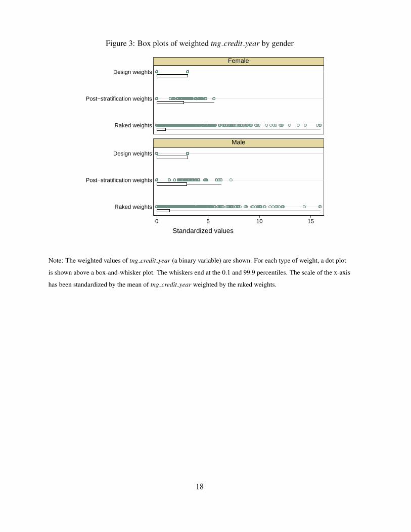
Figure 3: Box plots of weighted tng credit year by gender

Raked weights


Design weights

Raked weights


Design weights

0 5 10 15

Female

Male

Standardized values

Note: The weighted values of tng credit year (a binary variable) are shown. For each type of weight, a dot plot

is shown above a box-and-whisker plot. The whiskers end at the 0.1 and 99.9 percentiles. The scale of the x-axis

has been standardized by the mean of tng credit year weighted by the raked weights.

18

Table 1: 50th and 95th percentiles of weights

Design Weights Post-Stratification Weights Raked Weights

50th 95th 50th 95th 50th 95thOverall 7,235 7,235 7,128 10,395 4,221 25,169GenderFemale 7,235 7,235 7,128 10,395 4,088 23,616Male 7,235 7,235 7,060 11,278 4,365 25,917Age

18–34 7,235 7,235 7,606 14,012 5,173 29,46334–54 7,235 7,235 7,202 9,720 4,311 22,06555+ 7,235 7,235 7,060 9,207 3,520 25,917

Income<$45K 7,235 7,235 7,128 10,197 3,165 21,040

$45K–$85K 7,235 7,235 7,060 10,395 3,917 24,152$85K+ 7,235 7,235 7,202 10,700 7,293 38,298RegionAtlantic 7,235 7,235 7,202 10,700 7,293 38,298Quebec 7,235 7,235 6,616 9,061 3,701 23,849Ontario 7,235 7,235 6,464 10,395 3,789 22,198Prairies 7,235 7,235 7,427 9,872 4,486 26,150

BC 7,235 7,235 7,764 13,407 4,622 29,420PanelCFM 7,235 7,235 7,128 10,197 4,558 29,420

Non-CFM 7,235 7,235 7,128 10,395 4,814 24,180Online 7,235 7,235 7,128 10,395 3,704 22,126

* The panel or subsample refers to the way the respondents were recruited (CFM: recently responded to theCanadian Financial Monitor (CFM) survey and invited by regular mail; Non-CFM: selected from an offlinepanel of potential volunteers and invited by regular mail; Online: selected from an online panel of potentialvolunteers and invited by email).

Note: The 50th and 95th percentiles of design, post-stratification and raked weights are shown. Raked weights

are trimmed at five times their mean during the raking process.

19

Table 2: Total of cash on hand and tng credit year

Linearization Estimates* ResamplingEstimates

DesignWeights

Post-StratificationWeights

RakedWeights

RakedWeights

CASH ON HAND

Total 2.17E+09 1.00 1.02 1.02

Variance No Strata 9.79E+15 1.10 1.67 0.69

Variance Strata 9.67E+15 1.10 1.66 0.65

TNG CREDIT YEAR

Total 9.28E+06 1.02 0.93 0.93

Variance No Strata 4.31E+10 1.12 2.51 1.07

Variance Strata 4.15E+10 1.09 2.54 1.14

* Linearization estimates are produced with the linearization procedure in Stata, which simply assumesa stratified random sample and does not take into account the weighting procedure. Hence all of thelinearization variance estimates (for population totals) are calculated as

∑Lh=1(1−fh) nh

nh−1∑nh

i=1(yhi−yh)2, where L is the number of strata, nh is the number of primary sampling units (PSUs) in stratum h,(1 − fh) is the finite population correction for stratum h, fh is the sampling rate for stratum h, yhi isthe weighted value for PSU (h, i) and yh = 1

nh

∑nh

i=1 yhi (StataCorp 2013).

Note: All columns after the first have been divided by the value in the first column. The rows in italics show the

weighted point estimates, and all other rows show variance estimates. For example, the total cash on hand is

estimated to be 2.17E+09 under the design weights and 1.02*(2.17E+09) under the raked weights. The variance

for this estimate is 9.67E+15 under the design weights with the linearization method, taking into account the

strata, and 0.65*(9.67E+15) under raked weights with the resampling method, taking into account the strata.

Total number of contactless credit adopters is estimated by the weighted total of the binary variable

tng credit year. There are 3,663 respondents to the 2013 MOP survey, out of which 3,651 provided non-missing

data for cash on hand. Among these 3,651 consumers, 1,743 are males and 1,908 are females. There are 3,578

respondents who provided non-missing data for tng credit year. Among these 3,578 consumers, 1,699 are males

and 1,879 are females.

20

Table 3: Mean of cash on hand and tng credit year


DesignWeights


RakedWeights

RakedWeights

CASH ON HAND

Mean 81.96 1.00 1.03 1.03

Variance No Strata 14.02 1.09 1.51 0.85

Variance Strata 13.86 1.10 1.51 0.83

TNG CREDIT YEAR

Proportion 0.36 1.02 0.93 0.93

Variance No Strata 6.43E-05 1.08 2.10 1.24

Variance Strata 6.20E-05 1.09 2.15 1.20


∑Lh=1(1−fh) nh

nh−1∑nh

i=1(yhi−yh)2, where L is the number of strata, nh is the number of PSUs in stratum h, (1 − fh) is the finitepopulation correction for stratum h, fh is the sampling rate for stratum h, yhi is the weighted value forPSU (h, i), and yh = 1

nh

∑nh



weighted point estimates, and all other rows show variance estimates. The proportion of contactless credit

adopters is estimated by the weighted mean of the binary variable tng credit year. There are 3,663 respondents

to the 2013 MOP survey, out of which 3,651 provided non-missing data for cash on hand. Among these 3,651

consumers, 1,743 are males and 1,908 are females. There are 3,578 respondents who provided non-missing data

for tng credit year. Among these 3,578 consumers, 1,699 are males and 1,879 are females.

21

Table 4: Mean of cash on hand and tng credit year, by demographic category


DesignWeights


RakedWeights

RakedWeights

CASH ON HAND

GENDER

Female Mean 69.53 1.02 1.10 1.10


Variance Strata 25.97 1.29 1.65 0.97

Male Mean 95.57 0.98 0.98 0.98


Variance Strata 29.68 0.90 1.37 0.94

AGE

18–34 Mean 58.07 1.03 1.06 1.06


Variance Strata 19.01 1.34 4.96 2.61

34–54 Mean 68.54 1.01 1.02 1.02


Variance Strata 11.29 1.04 1.69 1.21

55+ Mean 112.91 1.00 1.05 1.05


Variance Strata 83.77 1.12 1.00 0.67

INCOME

<$45K Mean 74.99 1.00 1.01 1.01


Variance Strata 47.51 1.17 0.67 0.53

Continued on next page

22

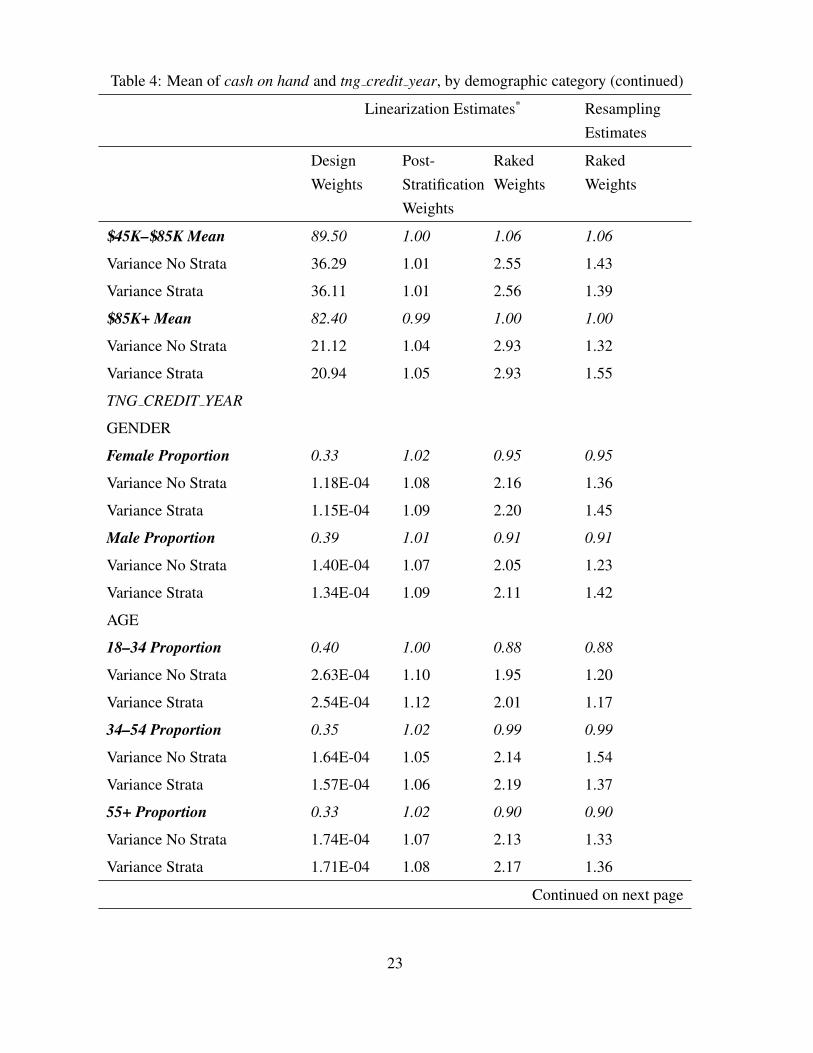
Table 4: Mean of cash on hand and tng credit year, by demographic category (continued)


DesignWeights


RakedWeights

RakedWeights

$45K–$85K Mean 89.50 1.00 1.06 1.06


Variance Strata 36.11 1.01 2.56 1.39

$85K+ Mean 82.40 0.99 1.00 1.00


Variance Strata 20.94 1.05 2.93 1.55

TNG CREDIT YEAR

GENDER

Female Proportion 0.33 1.02 0.95 0.95



Male Proportion 0.39 1.01 0.91 0.91



AGE

18–34 Proportion 0.40 1.00 0.88 0.88



34–54 Proportion 0.35 1.02 0.99 0.99



55+ Proportion 0.33 1.02 0.90 0.90




23

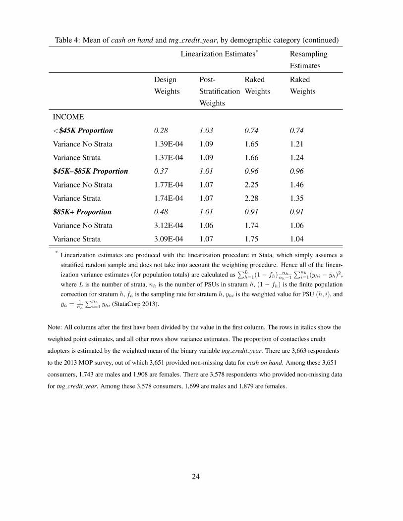
Table 4: Mean of cash on hand and tng credit year, by demographic category (continued)


DesignWeights


RakedWeights

RakedWeights

INCOME

<$45K Proportion 0.28 1.03 0.74 0.74



$45K–$85K Proportion 0.37 1.01 0.96 0.96



$85K+ Proportion 0.48 1.01 0.91 0.91



* Linearization estimates are produced with the linearization procedure in Stata, which simply assumes astratified random sample and does not take into account the weighting procedure. Hence all of the linear-ization variance estimates (for population totals) are calculated as

∑Lh=1(1 − fh) nh

nh−1∑nh

i=1(yhi − yh)2,where L is the number of strata, nh is the number of PSUs in stratum h, (1 − fh) is the finite populationcorrection for stratum h, fh is the sampling rate for stratum h, yhi is the weighted value for PSU (h, i), andyh = 1

nh

∑nh








24

Table 5: Mean of cash on hand and tng credit year, by region


DesignWeights


RakedWeights

RakedWeights

CASH ON HAND

Atlantic Mean 96.30 0.99 0.97 0.97


Variance Strata 418.01 0.92 0.56 0.53

Quebec Mean 85.47 1.02 0.89 0.89


Variance Strata 99.34 1.35 0.31 0.30

Ontario Mean 79.63 0.99 1.12 1.12


Variance Strata 28.38 1.02 3.62 1.84

Prairies Mean 80.74 1.00 1.08 1.08


Variance Strata 20.92 1.30 2.78 1.93

BC Mean 75.27 0.99 1.06 1.06


Variance Strata 24.86 0.99 2.61 1.41

TNG CREDIT YEAR

Atlantic Proportion 0.33 0.97 0.85 0.85



Quebec Proportion 0.26 1.03 0.92 0.92




25

Table 5: Mean of cash on hand and tng credit year, by region (continued)


DesignWeights


RakedWeights

RakedWeights

Ontario Proportion 0.45 1.00 0.94 0.94



Prairies Proportion 0.32 1.05 0.92 0.92



BC Proportion 0.36 1.01 0.91 0.91




∑Lh=1(1−fh) nh

nh−1∑nh


nh

∑nh








26

Table 6: Mean of cash on hand and tng credit year, by subsample


DesignWeights


RakedWeights

RakedWeights

CASH ON HAND

CFM Mean 84.01 1.00 0.99 0.99


Variance Strata 23.46 1.04 1.84 1.10

Non-CFM Mean 92.15 1.02 1.00 1.00


Variance Strata 150.45 1.21 0.39 0.30

Online Mean 75.46 0.99 1.08 1.08


Variance Strata 26.04 0.98 3.03 1.85

TNG CREDIT YEAR

CFM Proportion 0.39 1.01 0.89 0.89



Non-CFM Proportion 0.35 1.03 0.95 0.95



Online Proportion 0.33 1.02 0.95 0.95




∑Lh=1(1−fh) nh

nh−1∑nh


nh

∑nh


27






for tng credit year. Among these 3,578 consumers, 1,699 are males and 1,879 are females. The panel or

sub-sample refers to the way the respondents were recruited (CFM: recently responded to the Canadian Financial

Monitor (CFM) survey and invited by regular mail; Non-CFM: selected from an offline panel of potential

volunteers and invited by regular mail; Online: selected from an online panel of potential volunteers and invited

by email).

28

Appendix A Practical Implementation

We implement variance estimation in Stata, a popular statistical software package. Referringto Kolenikov (2010, 2014), we use the ipfraking and bsweights commands. Stata do-filesfor replicating our process, and results are available upon request. In Table A1, we comparethe Rake command in R with the ipfraking command in Stata so that similar results can bereproduced under R.

Step 1: Compute the initial post-stratification weightFirst, we must specify the strata and the initial weight with which to begin the raking pro-

cedure. The raking procedure will minimize the discrepancy between the raked weights andinitial weights. Here we set the initial weights to be the post-stratification weights basewgt,which equals the population stratum size divided by the number of respondents in the corres-ponding stratum. This basewgt variable will be declared in the argument [pw=varname] in theipfraking command, which generates the raked weights.

The weights are also declared when setting the survey environment in Stata. For example,the Stata output in Figure A1 shows an estimate of the cash on hand variable using the designweights. To obtain this estimate in Stata, we declare the weight variable as well as the strataused in the sampling design, which divide the population based on region, gender, and age.

Figure A2 shows the command for declaring post-stratification weights in Stata. The post-strata variable, strata, contains identifiers for the strata to be used, and the postweight variable,Count, contains the population counts for each stratum. Declaring these two variables is equi-valent to using basewgt, the variable containing the post-stratification weights.

Step 2: Generate the raked weightsNote that raked weights for the entire sample are necessary for generating replicate raking

weights. Besides the initial post-stratification weights, the ipfraking command also requires usto specify the population marginal totals of the control variables. Hence, as mentioned above,we refer to the weighting manual and select the “Econ Plus” set of variables recommendedin Vincent (2015), which are marital status nested within region; age category nested withinmobile phone ownership; age category nested within online purchase; income category nestedwithin education, gender, home ownership; and employment status nested within region.

We trim the weights at five times their mean to avoid extreme weights. Assuming the totalcalculated with the untrimmed weights to be the true value of total cash on hand, we computethe mean squared error (MSE) for weights trimmed at different values. Figure A3 shows theratios of these MSEs to the MSE of the total estimate with untrimmed weights, which is theestimated variance of the untrimmed total estimate for cash on hand. At truncation pointsabove five times the mean, the MSEs are all roughly equal to the MSE for the untrimmed

29

weights, and so trimming at five times the mean does not create a large difference in the MSE.In the ipfraking command, we set the tolerance between raked and control totals to 0.01

and the procedure converges in 11 iterations. The diagnostic plots (Figure A4 bottom panel)show that the discrepancies between weighted totals and control totals decrease rapidly andchange very little beyond the fourth or fifth iteration.

To test for robustness, we also rake with the tolerance at 0.001. In this case, the number ofiterations increases to 25. The weights change slightly but remain very similar to the weightswith tolerance 0.01, given that the correlation between the two sets of weights is about 1.00.The high correlation can be seen in Figure A5, a scatter plot of the weights generated withtolerance 0.01 and 0.001. A scatter plot of the weights generated by Stata and those generatedby R is shown in Figure A6. They are not as highly correlated because of the different ways inwhich trimming is performed in R and Stata (see Table A1).

Figure A7 shows the command used to produce the raked weights for the full data set,which can be divided into three subsamples based on method of recruitment. The rationale forraking after collapsing the subsamples into a single sample is offered in Appendix B. For moredetails on the raking procedure, see Vincent (2015).

Step 3: Generate the replicate raking weights using the bootstrapWe generate the replicate raking weights by calling ipfraking after bsweights

(Kolenikov 2010). Iterative proportional fitting is therefore performed on each bootstrappedsample after all the samples have been generated.

As shown in Figure A8, we specify the strata and initial post-stratification weights beforerunning bsweights so that the resampling procedure mimics stratified random sampling, usingthe same strata as the original survey design.

Figure A9 shows the bsweights command used to create 300 sets of replicate weights, withthe seed set to 2014. We choose to create 300 replicates based on Figure A10, which shows thevariance estimates of the mean of the variable cash on hand varying with respect to differentnumbers of bootstrap replications. Twenty trials were conducted for each replication size from50 to 1,000 in intervals of fifty, and box plots are produced of the resulting variance estimates.The variance estimates are stable with respect to the number of replications, with the medianestimates all approximately 13. Moreover, Figure A11 shows that with 300 replications, theaverage time to compute the variance is roughly 3 seconds.

Step 4: Declare the bootstrap survey environment in StataIn the declaration of survey environment, we specify the bootstrap option (vce[bootstrap])

and the names of the replicate weights (bsrw[bsw final 1-bsw final 300]) so that variances willbe calculated using the replicate raking weights. We then estimate the total value of the cash

on hand variable and its variance under the bootstrap environment (see Figure A12).

30

Figure A1: Estimating total value of cash on hand with strata under design weights

r; t=0.05 14:02:45

. gen simplewgt = 26502410/3663

r; t=0.00 14:02:45

. svyset [pw=simplewgt], strata(strata)

pweight: simplewgt

VCE: linearized

Single unit: missing

Strata 1: strata

SU 1: <observations>

FPC 1: <zero>

r; t=0.02 14:02:45

. svy: total cashonhand_ed

(running total on estimation sample)

Survey: Total estimation

Number of strata = 84 Number of obs = 3651

Number of PSUs = 3651 Population size = 26415588

Design df = 3567

Linearized

Total Std. Err. [95% Conf. Interval]

cashonhand_ed 2.17e+09 9.83e+07 1.97e+09 2.36e+09

r; t=0.08 14:02:45

Note: The total of cash on hand is estimated with design weights (see Step 1). The number of respondents with

non-missing values for cash on hand is 3,651.

31

Figure A2: Setting up a survey environment with post-stratification weights

r; t=0.06 14:02:46

. svyset [pw=simplewgt], strata(strata) poststrata(strata) postweight(Count)

pweight: simplewgt

VCE: linearized

Poststrata: strata

Postweight: Count


Strata 1: strata

SU 1: <observations>

FPC 1: <zero>

r; t=0.02 14:02:46

Note: The variable strata is the post-strata category and the variable Count contains the population size of each

post-stratum (see Step 1).

32

Figure A3: Ratios of mean squared errors for cash on hand using trimmed raked weights

01

23

45

Rat

io o

f mea

n sq

uare

d er

rors

2 4 6 8 10 12Truncation point for raked weights

Note: MSEs are calculated for the cash on hand variable taking the total computed with untrimmed weights to be

the true total (see Step 2). They are then divided by the MSE of the total estimate with untrimmed weights (which

equals the variance of the total estimate with untrimmed weights). The resulting ratios are plotted in Figure A3.

33

Figure A4: Diagnostic graphs for ipfraking with no trimming and optimization tolerance 0.01

01,

000

2,00

0F

requ

ency

0 10 20 30Standardized raked weights

01,

000

2,00

0F

requ

ency

0 5 10 15 20 25Adjustment factor

0.00.51.01.52.02.5

0 5 10Iteration

income_education

gender

home_ownership

employment_region

0.00010.0010.010.1

110

0 5 10Iteration

marital_region

age_mobile

age_online

Note: These graphs show the result of performing raking based on CIUS data (Step 2). Starting from the upper

left corner and moving clockwise, we have a histogram of the raked weights produced, a histogram of the ratio

between the raked weights and intial weights, a plot on a log scale showing the discrepancy with CIUS targets by

the number of iterations, and the same plot on an absolute scale. The scale on the x-axis of the histogram in the

upper left-hand corner has been standardized by the mean of the raked weights.

34

Figure A5: Scatter plot of untrimmed raked weights with tolerance 0.01 and tolerance 0.001

010

2030

Rak

ed w

eigh

ts w

ith to

lera

nce

0.00

1 (s

tand

ardi

zed)

0 10 20 30Raked weights with tolerance 0.01 (standardized)

Note: Both sets of weights have been standardized by the mean of the untrimmed raked weights with

tolerance 0.01 (see Step 2).

35

Figure A6: Scatter plot of trimmed raked weights generated from Stata and R

01

23

45

Trim

med

rak

ed w

eigh

ts fr

om S

tata

(st

anda

rdiz

ed)

0 1 2 3 4 5Trimmed raked weights from R (standardized)

Note: Both sets of weights have been standardized by the mean of the untrimmed raked weights generated from

Stata with tolerance 0.01 (see Step 2).

36

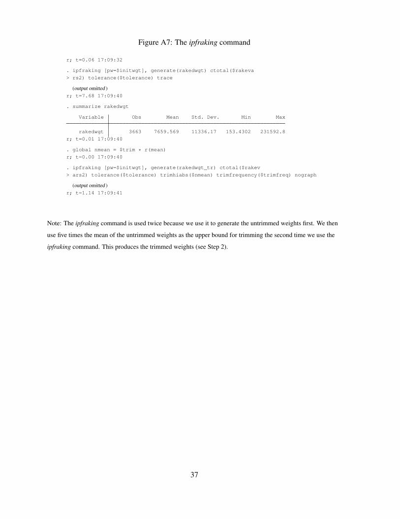
Figure A7: The ipfraking command

r; t=0.06 17:09:32

. ipfraking [pw=$initwgt], generate(rakedwgt) ctotal($rakeva

> rs2) tolerance($tolerance) trace

(output omitted )r; t=7.68 17:09:40

. summarize rakedwgt

Variable Obs Mean Std. Dev. Min Max

rakedwgt 3663 7659.569 11336.17 153.4302 231592.8

r; t=0.01 17:09:40

. global nmean = $trim * r(mean)

r; t=0.00 17:09:40

. ipfraking [pw=$initwgt], generate(rakedwgt_tr) ctotal($rakev

> ars2) tolerance($tolerance) trimhiabs($nmean) trimfrequency($trimfreq) nograph


Note: The ipfraking command is used twice because we use it to generate the untrimmed weights first. We then

use five times the mean of the untrimmed weights as the upper bound for trimming the second time we use the

ipfraking command. This produces the trimmed weights (see Step 2).

37

Figure A8: Specifying initial survey environment for bsweights

r; t=0.06 13:27:36

. svyset [pweight=$initwgt], strata(strata) psu(id)

pweight: basewgt

VCE: linearized


Strata 1: strata

SU 1: id

FPC 1: <zero>

r; t=0.00 13:27:36

Note:initwgt is a placeholder for the initial weight to be used for generating the bootstrap replicate weights

(see Step 3). In this case, it is the post-stratification weights.

38

Figure A9: The bsweights command

r; t=0.05 13:27:36

. set seed 2014

r; t=0.00 13:27:36

. bsweights bsw_, reps(300) n(-1) dots

Warning: the first-order balance was not achieved


. forvalues i=1/300{

2. ipfraking [pw=bsw_ì´], generate(bsw_untr_ì´) nograph

> ctotal($rakevars) tolerance($tolerance)

3. summarize bsw_untr_ì´

4. global nmean = $trim * r(mean)

5. ipfraking [pw=bsw_ì´], generate(bsw_final_ì´) nograph

> ctotal($rakevars) tolerance($tolerance) trimhiabs($nmean) trimfrequency($trimfreq)

6. }

Note: We first produce bootstrap replicate weights using the post-stratification weights as the initial weights.

We then calibrate each of the 300 sets of bootstrap replicate weights using the same raking procedure used for

the complete sample (Step 3).

39

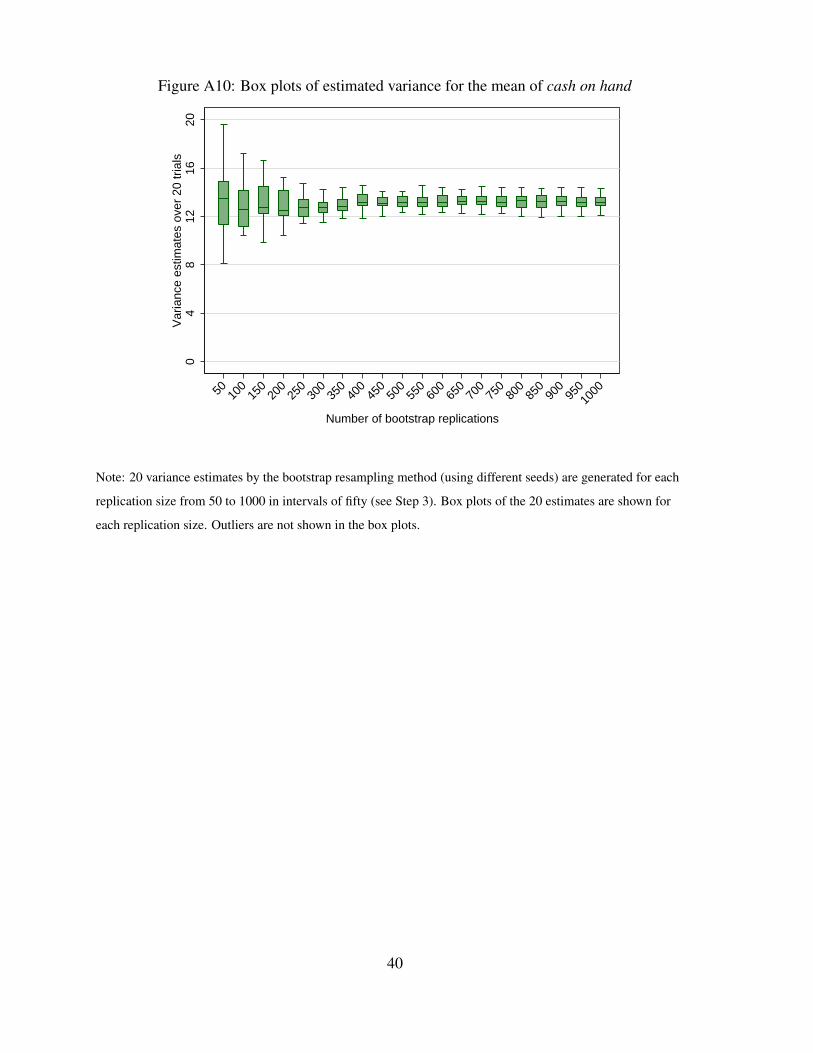
Figure A10: Box plots of estimated variance for the mean of cash on hand

04

812

1620

Var

ianc

e es

timat

es o

ver

20 tr

ials

50 100

150

200

250

300

350

400

450

500

550

600

650

700

750

800

850

900

95010

00

Number of bootstrap replications

Note: 20 variance estimates by the bootstrap resampling method (using different seeds) are generated for each

replication size from 50 to 1000 in intervals of fifty (see Step 3). Box plots of the 20 estimates are shown for

each replication size. Outliers are not shown in the box plots.

40

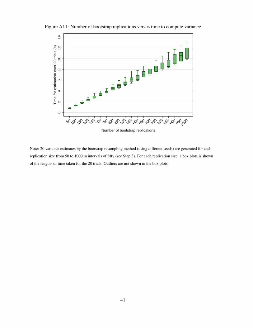
Figure A11: Number of bootstrap replications versus time to compute variance

02

46

810

1214

Tim

e fo

r es

timat

ion

over

20

tria

ls (

s)

50 100

150

200

250

300

350

400

450

500

550

600

650

700

750

800

850

900

95010

00

Number of bootstrap replications

Note: 20 variance estimates by the bootstrap resampling method (using different seeds) are generated for each

replication size from 50 to 1000 in intervals of fifty (see Step 3). For each replication size, a box plots is shown

of the lengths of time taken for the 20 trials. Outliers are not shown in the box plots.

41

Figure A12: Estimating total of cash on hand with replicate weights

r; t=0.05 14:02:46

. svyset [pw=rakedwgt_tr], vce(bootstrap) bsrw(bsw_final_1-bsw

> _final_300) dof(3570)


. svy: total cashonhand_ed

(running total on estimation sample)

Bootstrap replications (300)

1 2 3 4 5

.................................................. 50

.................................................. 100

.................................................. 150

.................................................. 200

.................................................. 250

.................................................. 300

Survey: Total estimation Number of obs = 3651

Population size = 26153773

Replications = 300

Design df = 3570

Observed Bootstrap Normal-based

Total Std. Err. [95% Conf. Interval]

cashonhand_ed 2.21e+09 7.95e+07 2.06e+09 2.37e+09

r; t=2.89 14:02:49

Note: The total of cash on hand is estimated using raked weights and the variance is estimated with the bootstrap

replicate weights (see Step 4). The number of respondents with non-missing values for cash on hand is 3,651.

42

Table A1: Comparison of the raking commands in R and Stata

Rake command in R ipfraking command in Stata

Convergence criteria Based on the followingmetric between suc-cessive iterative weights:maxj∈S |wk,pj /wk−1,pj − 1|,where wk,pj is the jth unitweight at the kth step. Con-vergence is declared whenthe metric falls below auser-specified tolerance level(Lumley 2012).

Similarly based on the iter-ative weights but also allowsuser to specify a tolerancelevel for matching margins.This tolerance level does notaffect convergence, but Stataissues a warning message if itis not satisfied.

Numerical solution Uses the Newton-Raphsonmethod with analytical deriv-atives (Lumley 2012).

Uses the Newton-Raphsonmethod with numerical deriv-atives.

The order of constraints Does not matter if processconverges.

Does not matter if processconverges.

Trimming Different options available:trimming after each iterationor trimming at end of rakingprocess. Does not redistributeweights to untrimmed obser-vations.

Trims at the end of theraking process and redistrib-utes trimmed weights to un-trimmed observations.

Note: The Rake command is from the R package survey written by Thomas Lumley. The ipfraking command is

from the Stata package ipfraking by Stanislav Kolenikov.

43

Appendix B Rationale for Collapsing Three Subsamples

The full 2013 MOP survey sample consists of three distinct subsamples: online (respond-ents selected from an online panel of potential volunteers and invited by email)9, offline CFM(recent participants of the Canadian Financial Monitor survey invited by regular mail), andNon-CFM (respondents selected from an offline panel of potential volunteers and invited byregular mail). In this section, we justify performing calibration on the full combined data setinstead of on the three subsamples separately.

Step 1: We compare both the missing patterns and the distributions of the completed SQquestions for the online, offline CFM, and Non-CFM subsamples, and we find the following:

• For the 2013 MOP survey, the offline CFM and offline Non-CFM respondents have loweritem-response rates than the online respondents. However, among offline respondents,CFM and Non-CFM respondents have similar missing data patterns.

• Regarding the distributions of answers to the survey questions, we find significant differ-ences between the online and offline respondents. Nevertheless, there are few differencesbetween the offline CFM and offline Non-CFM. For the completed survey questions, weconduct the two-sample omnibus test introduced by Epps and Singleton, which usuallyhas greater power and is suitable for both discrete and continuous valued data. How-ever, the Epps-Singleton test may fail when data are heavily concentrated in a singlevalue (almost degenerating to a constant), in which case we conduct the Mann–Whitneyrank-sum (MW) test instead.

Action: Combine the offline CFM and Non-CFM to generate the paper-based frame(to achieve a larger sample size and better MSE performance), while keeping the onlinesubsample as a separate frame.

Step 2: Perform the analysis suggested by Brick et al. (2006) and Young et al. (2012) tocompare the means and variances across different weighting schemes (see below).

• Based on the above discussion, we determine that we have a classical dual-frame sample.In particular, we have a non-overlapping dual-frame sample because panelists can onlybe invited once for the MOP survey, although they are allowed to be in both the paper-based and online subsamples. Ipsos Reid sent invites to the paper-based frame first, then

9 Probability sampling ensures that every possible sample from the population has a known probability of be-ing chosen (Lohr 2010). Because the online panel is not recruited using probability sampling, Bayesian credibilityintervals are usually calculated for estimates based on this panel (Roshwalb, El-Dash and Young 2012). However,in this report, frequentist variance estimation is used to measure the sampling errors for the pseudo-population(Quatember 2016) instead of for the true population.

44

de-duplicated those who had been invited from the paper-based when sending the onlineinvites. The advantage of a non-overlapping dual-frame sample is that we have a simpleway to collapse different frames and do not need to adjust for the composite weights asin an overlapping dual-frame sample (Callegaro et al. 2011).

• Option 1 Only use the design weights without the raking procedure: Obtain designweights for the paper-based frame as WD

P and the online frame as WDO , respectively.

Then merge the two frames with the weights{WDP ,W

DO

}. According to Vincent (2015),

we will produce two sets of design weights, which can be fed into the raking procedure.

• Option 2 Merge and then rake: Rake the combined data set with the initial weights{WD

P , WDO }, and this will generate the raked weights {WR

P , WRO }. A similar method

was implemented for two surveys: (1) Canadian Community Health Survey and (2) theSurvey Data on the Health of New Yorkers.

• Option 3 Rake separately for each frame, then merge: Rake each frame separately, withthe initial weights from Option 1. This will produce the raked weights {WR′

P } and {WR′O }

for the paper-based and online frames. Lastly we merge {WR′P } and {WR′

O } to generatethe merged weights {WR′

P ,WR′O }.

• Option 4 Merge and then rake with an extra Internet access control variable indicatingwhether the panelist has access to the Internet at home. Rake the combined data set withthe initial weights {WD

P , WDO } with an extra Internet access control variable, and this

will generate the raked weights {WRIP , WRI

O }.

• Option 5 Only rake the paper-based frame, producing the raked weights {WR′′P }.

Table B1 shows the means and variances of different weighting schemes with uniformweights as the initial weights for raking, while Table B2 is constructed similarly except usingpost-stratification weights for raking. In terms of weighted mean estimates, differences acrossweighting schemes are less than five percent. The differences between the estimated meansare similar even with different initial weights. As for the variances associated with differentweighting schemes, the variance from Option 2 is the second smallest in Table B1 and thesmallest in Table B2, suggesting that using the raking in the last step is able to reduce thevariance dramatically (D’Arrigo and Skinner 2010).

Action: Choose Option 2, which first merges the two frames and then applies the raking asfor the calibration of a full data set.

45

Table B1: Means and variances of cash on hand using uniform weights in raking

Option 1 (N/n) Option 2 Option 3 Option 4 Option 5

Mean 81.96 77.95 76.94 80.10 79.24

Variance 14.72 7.02 26.08 9.22 6.34

Note: Variance of Option 1 is calculated based on the linearization method, which is the default in Stata, while

variance estimates from Options 2 to 5 are computed based on the bootstrap resampling.

Table B2: Means and variances of cash on hand using post-stratification weights in raking

Option 1 (Nh/nh) Option 2 Option 3 Option 4 Option 5

Mean 81.91 78.27 76.91 79.94 82.25

Variance 16.76 7.13 56.27 9.33 11.78

Note: Variance of Option 1 is calculated based on the linearization method, which is the default in Stata, while

variance estimates from Options 2 to 5 are computed based on the bootstrap resampling.

46

Documents

Variance Estimation for Survey-Weighted Data Using ... · Variance Estimation for Survey-Weighted Data Using Bootstrap Resampling Methods: 2013 Methods-of-Payment Survey ... approximate