Validation of qualitative for discussion June€¦ · validation of qualitative and semi quantitative (screening) methods by collaborative trial: a harmonized protocol) chaired by

1

A PROTOCOL FOR THE VALIDATION OF QUALITATIVE METHODS OF

ANALYSIS

Roy Macarthur

Food and Environment Research Agency, Risk and Numerical Sciences Team, Sand

Hutton, YO41 1LZ York, United Kingdom

Christoph von Holst

European Commission, Joint Research Centre, Institute for Reference Materials and

Measurements (EC-JRC-IRMM), Retieseweg 111, B-2440 Geel, Belgium

2

Abstract

This paper presents a draft protocol for analyzing the results of validation studies for

qualitative methods of analysis which is designed to meet three competing goals: 1)

to give correct answers; 2) have a broad scope of application; and 3) be accessible

to a wide range of users.

The draft protocol can be applied to the validation of methods by collaborative trial or

to single-laboratory studies. The protocol produces an estimate of the probability of a

positive response with a confidence interval within which 95% of laboratories (or

analytical runs) are expected to fall when the method is applied in practice. The

interval is calculated from the observed reproducibility (or within-laboratory

reproducibility) standard deviation. Then a simple plot of confidence intervals for the

probability of detection against the concentration of analyte is used to provide an

estimate of the range of limits of detection and false positive probability that we can

expect to see when the validated method is applied in practice. Use of the draft

protocol is demonstrated using results produced by three collaborative trials. A

simulation study showed that a conclusion that a method is fit for purpose that is

generated by the draft protocol is likely to be safe.

3

Introduction

A qualitative analytical method is one whose response can be interpreted as

“detected” or “not detected”, this may be because a response is inherently

qualitative, or where the response is quantitative it is uncorrelated (or very weakly

correlated with a short range of responses) with the quantity of analyte present in a

sample. Methods that deliver qualitative responses are commonly applied in many

analytical areas. For example rapid test methods, including qualitative tests are used

for the detection of microbiological contaminants, heavy metals, pesticides, foreign

bodies, mycotoxins, allergens and other analytes in food [1]. Their use, and in

particular their use by producers and consumers to test food and other products

against legislative of contractual limits, or by competent authorities for sanitary or

phytosanitray purposes, means that an internationally agreed guideline for validating

the performance of methods is needed. For quantitative methods the

IUPAC/AOAC/ISO Harmonized protocol [2] describes how to run validation studies,

and how to analyze results to describe important aspects of method performance,

although further work to clarify the relation between concentration and performance

may be required to validate methods against the specific requirements of the

decision-makers who use analytical results [3, 4, 5]. No internationally accepted

guidance on the validation of qualitative methods exists.

In 2006 IUPAC initiated a project to develop guidance for the validation of qualitative

methods (IUPAC project 2005-024-2-600 Establishment of guidelines for the

validation of qualitative and semi quantitative (screening) methods by collaborative

trial: a harmonized protocol) chaired by the European Commission’s Institute for

Reference Materials and Measurements. The project became more active from 2008

onwards with the involvement of more experts and the use of real-world validation

studies via co-operation with European projects: (1) Safeedpap (SAFEED-PAP

(FOOD-CT-2006-036221, European Commission), on the “Detection of presence of

species-specific processed animal proteins in animal feed”

http://safeedpap.feedsafety.org/) and (2) MoniQA (Monitoring and Quality Assurance

in the Food Supply Chain, Food-CT-2006-036337, European Commission,

http://www.moniqa.org/). This paper describes a draft protocol for the design of

validation studies and the analysis of results to produce a description of method

performance that directly meet the needs of users and decision-makers.

4

The aim of method validation for qualitative testing

When we use a qualitative method of analysis and we get a positive result we want

to be able to say with confidence that the analyte is present in the sample that we

tested. If we get a negative result then we want to be able to say with confidence that

if the analyte is present at all in the sample we tested then it must be at a

concentration below a specified low level. This is the purpose of qualitative testing.

The goal of validation of an analytical method is to provide assurance that a method

is likely to produce results that are fit for purpose. For qualitative methods two

quantities describe fitness for the purpose described above: 1) the probability that a

sample in which the analyte is absent will generate a negative response, and 2) the

lowest concentration for which the probability of a positive response is sufficiently

high (alternatively, the probability of a positive response for a given target

concentration of analyte). It is worth highlighting a few points about method

validation here:

1) A method validation study provides a prediction about the performance we

can expect to see when a method is applied in practice.

2) Analytical methods with the same probability of detection under the same

conditions are equivalent. For qualitative methods variation in performance

means a difference in the probability of detection.

3) To assess a qualitative method’s fitness for purpose as defined above, the

most generally useful description of the performance is the relationship

between the probability of detection and quantity of analyte.

4) Hence, the goal of method validation can be achieved by producing an

estimate of the probability of detection across a range of quantities of analyte

with a interval that gives a prediction interval within which the probability is

likely to lie when a method is applied in a new laboratory (for multi-laboratory

studies), on a new day or with a new matrix etc. (for single-laboratory studies).

Traditional and standard statistical approaches to validation

A traditional approach to assessing the performance of a qualitative methods is

based on the analysis of samples which are known to be ‘positive’ and samples

which are known to be ‘negative’ and simply reporting the proportion of positive

samples that give positive responses, called the sensitivity of the method (or its

5

inverse the false negative rate), and the proportion of negative samples which give a

negative response, called the specificity of the method (or its inverse the false

positive rate). This approach may be most useful where the target of the analysis

itself is intrinsically qualitative such as disease status or pregnancy. However it does

not meet our needs for validation of a qualitative method of analysis because while

there is no such thing as “a little bit pregnant” a sample may contain “a little bit of a

substance” or it may contain a larger quantity of a substance. Hence, the

performance of qualitative methods used to detect the presence of a substance will

depend upon, and should be considered with, the quantity of analyte in samples.

A standard statistical approach to examining the relationship between a quantity and

a qualitative response (often a biological response) whose probability of occurrence

depends on the quantity is through a regression using a generalized linear model

(GLM), often using a logit or probit link function [6]. There are two significant

challenges for non-statisticians who try to use this approach for the validation of

qualitative methods of analysis. The first challenge is that in general we do not know

the shape of the relationship between the probability of detection and the quantity of

an analyte. This means that the standard statistical approach requires some

exploratory non-linear modeling to identify the right (or good enough) transformation

and link function [6] before it can be applied to a particular set of results. The second

challenge, which is also a challenge for statisticians, is that it is difficult to get to a

prediction interval using these methods. In practice this means that we can use the

standard statistical methods to get an estimate of the relation between the expected

average probability of detection and quantity of analyte, but it is difficult to use them

to get at the range of probabilities of detection that we might see when new

laboratories use a method that has been validated in a collaborative trial, or when we

use a qualitative method tomorrow that was validated in-house today.

Recent approaches to validation

Langton et al introduced the idea of using accordance (the proportion of pairs of

samples give the same response when analyzed under repeatability conditions) and

concordance (the proportion of pairs of samples that give the same response when

analyzed under reproducibility conditions) as measures of variation in qualitative

response [7]. A particular strength of this approach is that it gives an intuitively

graspable feel for how conclusive a single test result is, or whether undertaking more

6

tests might yield more information. The approach was modified by van der Voet and

van Raamsdonk [8].

Wilrich and Wilrich have produced a method which is an example of the GLM-based

standard statistical approach [9]. It is designed to be specifically applicable to

microbiological qualitative tests in which the two sources of variation are the

presence or absence of colony forming units in a test aliquot and variation in the

probability of detection if organism is present which may be related to, for example,

the nature of the matrix. This method allows a relation between the average

probability of detection for each matrix and quantity of colony forming units to be

easily calculated. The size of uncertainty about the average probability of detection

for each matrix is also estimated.

Wilrich has also produced a method for estimating reproducibility and repeatability

standard deviations which treats qualitative results as quantitative results with value

“0” or “1” [10]. An analysis of variance, similar to that used to produce estimates of

reproducibility and repeatability for quantitative analytical results (based on ISO

5725), is then applied to allow three quantities to be estimated: 1) the average

probability of detection, 2) the average repeatability standard deviation of responses

and 3) the between-laboratory standard deviation of responses. Methods for

detecting significant between-laboratory variation and producing an approximate

prediction interval (based on a normal approximation) for the performance of new

laboratories are given. Wilrich remarks that both the observed average probability of

detection and estimated average repeatability standard deviation are artefacts,

because no individual laboratory actually has average performance; the repeatability

standard deviation for each laboratory is a function of the probability of detection for

that laboratory and the number of replicate analyses used to estimate it and that, in

contrast with quantitative analyses, it is difficult for most users to understand what

values of repeatability and reproducibility standard deviation really mean.

Wilrich suggests that it may be fruitful to consider the response of qualitative

methods in a more explicitly quantitative manner as the proportion of a number (he

suggests a minimum of 10) of replicate analyses which give a positive result, i.e. that

we should understand the ‘response’ of qualitative methods as a single observed

probability of detection rather than a set of replicate qualitative individual positive or

negative results. If we use this approach ‘repeatability’ variation is expressed as a

7

quantity which describes uncertainty about our single estimate of the probability of

detection for an individual laboratory and reproducibility standard deviation is

estimated by the observed standard deviation across laboratories which includes

contributions from between-laboratory variation and the uncertainty associated with

the estimated probability of detection in each laboratory.

Wehling et. al. [11] produced a protocol for the validation of qualitative methods

which also includes the application of the “ISO 5725 approach” to qualitative results,

coded as the quantitative results “1” and “0”, to get estimates of average repeatability

standard deviation and reproducibility standard deviation. Methods for producing

confidence intervals for the average probability of detection are based on a modified

Wilson interval (introduced by LaBudde [12]) for single-laboratory data and high and

low probabilities of detection for multi-laboratory data, and a normal approximation

for multi-laboratory data where the estimated probability of detection is closer to

50%. There is a strong focus on the use of the probability of detection to characterize

method performance in place of the traditional measures of qualitative performance,

and the use of graphs of the probability of detection against the quantity of analyte to

aid the interpretation of results.

Some points that we take from our reading of this recent work are:

1) Confirmation that the relation between probability of detection and quantity of

analyte is the most generally useful description of qualitative method

performance.

2) While the calculation of estimates for repeatability and reproducibility standard

deviations is as simple for individual qualitative results as it is for quantitative

results, the use of ‘repeatability standard deviation’ as a measure of method

variation is problematic and the interpretation of what a particular value of

reproducibility standard deviation means is not as intuitive as it is for

quantitative results.

3) There is a lack of harmony about how the effect of between-laboratory

variation should be described. One approach estimates the uncertainty about

the global average probability of detection; another approach estimates an

interval within which we can expect the performance of a high proportion of

individual laboratories to lie.

8

4) Replicate analysis of a set of samples within a laboratory provides a single

estimate of the probability of detection for that laboratory. Hence, a simple

standard deviation, across laboratories, of these estimates will provide an

estimate of the reproducibility standard deviation of the probability of

detection.

5) Using the normal approximation to calculate confidence intervals works best

for probabilities close to 0.5, but will give intervals which are too short at the

lower end for probabilities close to 1 and too short at the upper end for

probabilities close to 0. Because these are precisely the intervals that are of

most relevance to the validation of qualitative methods a more plausible

distribution should be used such as the beta distribution [13].

6) Graphical representations of method performance are much more informative

than estimates of parameters describing method performance for most users.

A standard protocol for qualitative method validation

The protocol presented in this paper is based on the calculation of performance

characteristics as intervals within which we expect the great majority (95%) of

individual laboratory’s performances to lie. This is important for method validation

because we want validated methods to perform well enough, with the claimed limit

of detection, in all laboratories that use them. This is in common with Wilrich[10] and

in contrast to Wehling et. al.[11] which uses estimates of the mean probability of

detection to describe performance.

The aim of this paper is to propose a protocol as a candidate to become a standard

protocol for the validation of qualitative methods of analysis. In common with

standard methods of analysis [5] the features we require of the protocol are that it

provides a way of meeting the goals of validation (gives estimates of 1: the

probability that a sample in which the analyte is absent will generate a negative

response, and 2: the lowest concentration for which the probability of a positive

response is sufficiently high) that is sufficiently robust so that it can be applied in a

wide range of situations, simple enough to be used by everyone who needs to, and

not requiring the use of particular equipment or software. Hence, like all standard

methods, this proposed protocol is a compromise between technical correctness,

wide scope of application and simplicity.

9

The validation protocol is designed to be applied to results generated by

collaborative trial and single-laboratory studies. It provides an estimate of the

relationship between the quantity of analyte and the probability of detection with an

interval within which we can expect the probability to lie when the method is used in

practice. We can then use the resulting graphical probability profile to explore the

relationship between false positive rate and limit of detection, to demonstrate

whether a method is likely to produce results that are fit for purpose, and to consider

the relative contributions to uncertainty made by variation in method performance

and the uncertainty associated with the analysis of a finite number of samples. The

protocol is focused on providing information that is of immediate value to users of

analytical methods for meeting the goals of method validation. An absolute minimum

protocol (smallest number of samples) is also provided. This can be used to test

whether a method meets a fitness for purpose requirement for false positive

probability and limit of detection, but it will not allow users to determine a limit of

detection for a method that narrowly fails to meet the fitness for purpose requirement

nor will it give any indication that a limit of detection is much lower than the required

target.

The candidate protocol

The basic study design and the analysis of results are similar for validation by multi-

laboratory or single laboratory study. The validation study should be preceded by

some preliminary work to give an indication of what kind of design is best (minimum

or larger) and over what kind of concentration range is the study likely to produce

informative results. The validation protocol proceeds as follows:

1) For multi-laboratory studies a set of blind-replicate samples is sent to each

laboratory. Sets of n blind-replicate samples, each set at one of a range of

concentrations between zero to some level above the target limit of detection,

are sent to a number (L) laboratories.

2) Samples are analyzed in each laboratory under repeatability conditions and

the results reported. Where a method gives a quantitative response (e.g.

intensity of color change) this should also be reported.

3) Results are used estimate a prediction interval for the probability of detection

when the method is applied in a new laboratory at each concentration.

10

4) Prediction intervals are plotted to estimate upper and lower limits for the limit

of detection and false positive probability.

5) A method has demonstrated unequivocally that it is very likely to produce fit

for purpose results when upper limits for prediction intervals for false positive

probability and limit of detection are no greater than their target values.

6) Confidence intervals for the probability of detection per laboratory based on

zero between-laboratory variation are estimated. These are used to examine

the relative impact of between-laboratory variation and the limited number of

analyses undertaken per laboratory on the variation of results. This can be

used to consider whether further analyses are likely to improve estimates of

false positive probability and limit of detection.

7) The absolute minimum design requires n blind-replicate samples that do not

contain the analyte, and m blind-replicate samples that contain the analyte at

a concentration no higher than the target limit of detection sent to each of L

laboratories such that nL negative results confirm that the false negative

probability is sufficiently low and mL positive results confirm that the false

negative probability at the limit of detection is sufficiently low.

Each of L laboratories reports the number of positive results xi out of ni tests per

laboratory (i=1,2,…L). Where a detection decision is made by applying a critical

value to a quantitative response, report the critical value and the response for each

test.

Hence at each concentration the estimated probability of detection for each

laboratory �� is given by �� ⁄ and the estimated probability of detection across

laboratories �� is given by

�� ⁄��

��

Equation 1

Calculate the observed standard deviation s across the values of pi (i=1 to L). This

includes the contribution from between laboratory variation in the probability of

detection and uncertainty about the probability of detection in each laboratory which

is associated with the finite number of replicate analyses used to estimate each

probability.

11

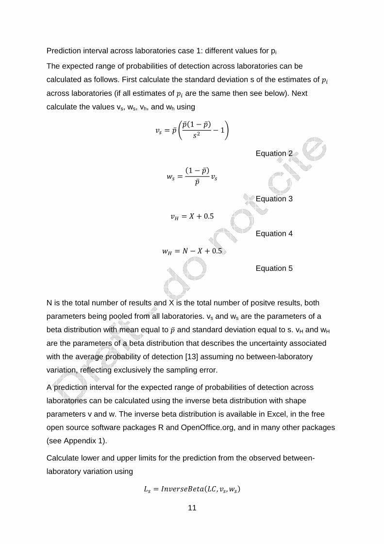
Prediction interval across laboratories case 1: different values for pi

The expected range of probabilities of detection across laboratories can be

calculated as follows. First calculate the standard deviation s of the estimates of �� across laboratories (if all estimates of �� are the same then see below). Next

calculate the values vs, ws, vh, and wh using

� � �� 1 � �� 1�

Equation 2

�� 1 � ��

Equation 3

� � � � 0.5

Equation 4

�� 0.5

Equation 5

N is the total number of results and X is the total number of positve results, both

parameters being pooled from all laboratories. vs and ws are the parameters of a

beta distribution with mean equal to �� and standard deviation equal to s. vH and wH

are the parameters of a beta distribution that describes the uncertainty associated

with the average probability of detection [13] assuming no between-laboratory

variation, reflecting exclusively the sampling error.

A prediction interval for the expected range of probabilities of detection across

laboratories can be calculated using the inverse beta distribution with shape

parameters v and w. The inverse beta distribution is available in Excel, in the free

open source software packages R and OpenOffice.org, and in many other packages

(see Appendix 1).

Calculate lower and upper limits for the prediction from the observed between-

laboratory variation using

� � �� !� " #$�%, �, ��

12

Equation 6

'� � �� !� " #$�'%, �, ��,

Equation 7

and from the pure sampling error using

� � �� !� " #$�%, � , ��

Equation 8

'� � �� !� " #$�'%, �, ��

Equation 9

Where LC is the percentile value of the lower end of a confidence interval (usually

5%) and UC is the percentile value of the upper end of a confidence interval (usually

95%).

and then

()� !(*+*# � +*�*+,+��, ��

Equation 10

,�� !(*+*# � +$�*+,+�'�, '��

Equation 11

Hence upper limits are taken as the maximum of the estimated upper end of the

confidence intervals (equation 7 or 9) for the average probability of detection

calculated by equation 1 and the probability of detection in a single laboratory, lower

limits are taken as the minimum of the estimated lower end of the confidence

intervals (equation 6 or 8) for the average probability of detection and the probability

of detection in a single laboratory.

Range across laboratories case 2: all pi=0 or all pi=1.

All laboratories participating in a trial may achieve 100% positive results for samples

containing higher concentrations of analyte and, for a good method, 100% negative

results for samples that do not contain the analyte. For these sets of results use [13]

13

for �� 1

()� !(*+*# � %- .⁄

Equation 10b

,�� !(*+*# � 1

Equation 11b

for �� 0

()� !(*+*# � 0

Equation 10c

,�� !(*+*# � 1 � �1 � '%�- .⁄

Equation 11c

Plotting the prediction intervals

The performance of the analytical method is described graphically by plotting results,

the limits for probabilities of detection and using these to estimate the values of the

limit of detection and false positive probability, as shown in Figure 1 to 3.

1) For each concentration plot the estimates of the probability of detection in

each laboratory p1, p2,… pL, (Figure 1)

2) plot ��, upperlimit and lowerlimit and join the averages and limits across

concentrations by linear interpolation (Figure 2)

3) The estimated average false positive probability is given by the intercept of

the �� line on the y-axis. The upper 95% confidence for the false positive

probability in an individual line is given by the intercept of the upperlimit line

on the y-intercept (0.032 in Figure 3). The estimated average limit of detection

is given by the concentration at which the �� line crosses the required

probability of detection. For instance, at 95 % confidence level, the estimated

average limit of detection is 0.089 % MBM (Figure 3). The estimated upper

14

95% confidence interval for the limit of detection in an individual laboratory is

given by the concentration at which the lowerlimit line crosses the required

probability of detection. (0.122% MBM in Figure 3)

Assessment of between laboratory variation

4) The variation displayed by estimates of the probability of detection across

laboratories (s) has two sources: between laboratory variation sL and the

binomial sampling variation associated with the finite number of analyses

used to estimate pi (sB). The use of an analysis of variance to test whether

there is significant between-laboratory variation is demonstrated by Wilrich

[10] and Wehling at al [11].

An alternative graphical approach is used here where an interval is plotted

which gives the variation we can expect to see in results if there is no

between-laboratory variation; the probability of variation in all laboratories is

equal to the average probability of detection across laboratories; and the

observed variation in probability of detection is just what we would expect to

see when using a small number of tests to estimate it in each laboratory. The

size of the interval is estimated using the beta-binomial distribution (Appendix

2) which gives estimates of confidence intervals for the number of positive

results xL (lower limit) and xU (upper limit) per laboratory where there is no

between-laboratory variation. Plot �� ⁄ and �/ �⁄ at each concentration level,

where n is the number of analyses per laboratory (Figure 4).

Comparison of the interval given by �� ⁄ and �/ �⁄ and upperlimit and

lowerlimt enables a direct assessment of the contribution to variation in results

made by between-laboratory variation and the study design, and whether

increasing the number of replicates might change the conclusions drawn from

the validation study. For example, where all or much of the variation comes

from the study design, �� ⁄ 0 ()� !(*+*# and �/ �⁄ 0 ,�� !(*+*# and we may

conclude that increasing the number of analyses will lead to better estimates

of the probability of detection.

15

5) Report a) the scope of the validation, b) estimates of likely range of false

positive rates and limits of detection when the method is used in practice c) an

opinion on whether undertaking further analyses is likely to change the

conclusions of the study.

6) For results from an absolute minimum study design calculate the mean upper

(5%) and lower (95%) limits of the prediction interval for the false positive

probability and probability of detection at the target limit of detection using

Equations 1 to 11

Examples

Example 1: Detection of meat and bone meal in animal feed

A collaborative trial (18 laboratories, 20 replicate samples at 7 levels including zero)

of a PCR-based method to detect the presence of meat and bone meal (MBM) in

animal feed yielded the following results (Table 1).

Note that we do not recommend that validation results are reported using the format of Table 1

because information about the performance of individual laboratories is lost. This format is

used here because it is a compact way of giving data which can be reconstituted to allow

readers of this paper to repeat the data analysis methods used in the draft validation protocol.

For example Table 2 gives reconstituted results for results produced by the analysis of

samples containing 0.01% MBM.

Table 2 shows an example of individual test results, reconstituted from Table 1,

which can be used as inputs for the candidate validation protocol.

Table 3 and 4 show the results of applying Equations 1 to 11 from the draft protocol

to results reconstituted from Table 1.

Figures 1 – 3, which we used to illustrate the draft protocol, are based on this

example. Figure 1 shows the observed probabilities of detection for laboratories

across the seven concentrations of MBM used in the validation study. Figure 3

shows that the observed probabilities of detection tell us that we can expect limits of

detection for individual laboratories using this method to be no higher (95%

confidence) than 0.12 % MBM extracted from animal feed and may be as low as

0.036% MBM extracted from animal feed for some laboratories. We can expect that

the false positive probability will be less than 0.032 for 95% of laboratories.

16

Figure 4 shows that there is more variation in results than can be explained by the

uncertainty about the mean probability of detection and binomial sampling variation

associated with 20 replicates per laboratory for samples containing up to 0.1% MBM.

Hence, the size of the interval within which the limit of detection may lie is likely to be

driven by variation in method performance (probability of detection changing

between laboratories) rather than uncertainty about performance that could be

reduced by further measurements.

Example 2: Detection of peanut protein

A collaborative trial (18 laboratories, 5 replicate samples at 7 levels including zero) of

a dipstick to test to an allergen (peanut) in cookies [14] yielded the following results

(Table 5).

Estimates of statistical parameters and prediction intervals for the probability of a

positive response are shown in Tables 6 and 7

Figure 5 shows that the observed probabilities of detection tell us that we can expect

limits of detection for individual laboratories using this method to be no higher (95%

confidence) than 29 mg/kg peanut in cookies, and may be as low as 13 mg/kg in

some laboratories. We can expect that the false positive probability will be less than

0.14 for 95% of laboratories.

Figure 6 shows that a large part of the observed variation can be explained by the

uncertainty about the mean probability of detection and the binomial sampling

variation associated with 5 replicates per laboratory for most concentrations. Hence,

if the uncertainty associated with the estimated limit of detection is too large then

estimates of method performance may be improved by undertaking further studies

using more replicate samples. This might be the case if the target limit of detection

were around 20 mg/kg.

The effect of the low number of replicates is particularly clear for results produced by

the analysis of cookies that did not contain peanut. Here the 2 out of 90 samples

gave a positive response, giving an estimated average false positive probability of

0.022 with a 95% confidence interval of 0.005 to 0.069. The problem is that the

estimated probability of a positive response for those two laboratories that each

produced a single positive response is 0.2, and these high estimates have a big

impact on the upper limit for the estimated probability of detection. In short the

17

results are consistent with a low-between-laboratory-variation false positive

probability of less than 1% (probably good enough for a screening method), or a

much higher (estimated upper 95% interval of 0.14) false positive rate for some

laboratories, and we can’t tell the difference because the number of replicates per

laboratory is low. In order to defend against these kinds of outcomes where

preliminary work leads to the expectation of a few false positive, or false negative

results a larger number of replicate analyses should be undertaken in each

laboratory (see Assessment of draft protocol performance and study design).

Example 3: A collaborative trial for the detection of salmonella in ground beef

A collaborative trial (11 laboratories, 6 replicate samples at 3 levels including zero) of

a method for the detection of salmonella in ground beef [11] yielded the following

results (Table 8), following the removal of results produced by one laboratory whose

performance was judged to be inconsistent with the other laboratories.

Calculation of the upper and lower limits (5 and 95%) for estimated probability of

detection at each concentration is shown in Tables 9 and 10. We were unable to use

the results to provide an estimate of the limit of detection where the mean probability

of detection was 95% or an upper limit for the expected limit of detection when the

method is applied in a new laboratory (Figure 7). We were able to estimate that the

limit of detection, when the method is applied in a new laboratory, can be expected

(95% confidence) to be higher than 8 cfu/25g and that the false positive probability

was likely (95% confidence) to be less than 0.05.

The observed variation between laboratories can be explained by the uncertainty

about the mean probability of detection and the binomial sampling variation

associated with 6 replicates per laboratory for all concentrations (Figure 8). Hence

estimates of method performance may be improved by undertaking further studies

using more replicate samples, possibly including some higher concentration

samples. However, we can’t be confident that this will be fruitful unless a limit of

detection larger than 8 cfu/25g is considered fit for purpose.

18

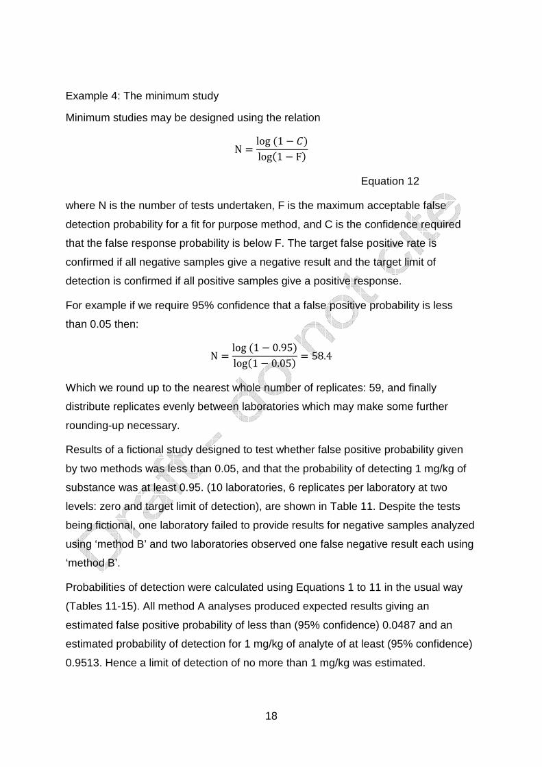
Example 4: The minimum study

Minimum studies may be designed using the relation

N � log �1 � %�log�1 � F�

Equation 12

where N is the number of tests undertaken, F is the maximum acceptable false

detection probability for a fit for purpose method, and C is the confidence required

that the false response probability is below F. The target false positive rate is

confirmed if all negative samples give a negative result and the target limit of

detection is confirmed if all positive samples give a positive response.

For example if we require 95% confidence that a false positive probability is less

than 0.05 then:

N � log �1 � 0.95�log�1 � 0.05� � 58.4

Which we round up to the nearest whole number of replicates: 59, and finally

distribute replicates evenly between laboratories which may make some further

rounding-up necessary.

Results of a fictional study designed to test whether false positive probability given

by two methods was less than 0.05, and that the probability of detecting 1 mg/kg of

substance was at least 0.95. (10 laboratories, 6 replicates per laboratory at two

levels: zero and target limit of detection), are shown in Table 11. Despite the tests

being fictional, one laboratory failed to provide results for negative samples analyzed

using ‘method B’ and two laboratories observed one false negative result each using

‘method B’.

Probabilities of detection were calculated using Equations 1 to 11 in the usual way

(Tables 11-15). All method A analyses produced expected results giving an

estimated false positive probability of less than (95% confidence) 0.0487 and an

estimated probability of detection for 1 mg/kg of analyte of at least (95% confidence)

0.9513. Hence a limit of detection of no more than 1 mg/kg was estimated.

19

The missing results from one laboratory using method B mean that the results do not

confirm that the false positive probability is less than 0.05. Similarly the two negative

responses produced by the analysis of the positive samples have a large effect on

the estimated range of values for the probability of detection that we may expect to

see when the method is used in practice (95% confidence interval 0.82 – 1.00).

Hence the ‘absolute minimum design’ is most useful where both the false positive

probability and false negative probability at the target limit of detection are thought to

be low enough such that one or more unexpected result is unlikely. Low enough

means very-close-to-zero, e.g. less than 0.0005 where 60 samples are analyzed at

the limit of detection and zero concentrations.

Assessment of draft protocol performance and validation study size

We assessed the performance of the draft protocol, and how it is influenced by

validation study size, by examining how well the upper 95% confidence limit of the

estimated probability of a positive response represented the expected 95th percentile

of simulated laboratories. This gave us an estimate of how reliable the upper limit of

the estimated false positive probability would be when assessing the fitness for

purpose of the method. By symmetry, this also gave us an estimate of how reliable

the lower limit of the estimated probability of detection (at high probabilities) would

be when used to estimate an upper limit for the limit of detection.

We used a number of scenarios. Each scenario consisted of an average probability

of a positive response (0.1, 0.05, 0.01) with beta-distributed between-laboratory

variation such that the probability of a positive response at the 95th percentile of

laboratories was at double the average (0.2, 0.1, 0.02). The protocol was applied to

each scenario using a range of numbers of laboratories (5, 10, 15, 20, 30, 50, 100)

and replicate analyses within each laboratory (5, 10, 20, 50, 100). Parameters

describing the scenarios are given in Table 16.

The simulation algorithm was

For each number of laboratories (L=5, 10, 15, 20, 30, 50, 100), number of

replicates per laboratory (n=5, 10, 20, 50, 100), and scenario (��=0.1, 0.05,

0.01)

20

Generate a probability of detection for each laboratory pi (i=1 to L) by

selecting a random value from the beta distribution.

Generate a number of positive and negative responses from n Bernouli

trials per laboratory with probability pi (i=1 to L).

Analyze the responses using the draft protocol

Report the estimated probability of a positive response for the upper

95th percentile of laboratories.

10000 estimates of probability of a positive response for the upper 95th percentile of

laboratories were produced for each scenario and study design, which were

summarized by their mean (solid line) , 5th and 95th percentile (dotted lines). (Figures

9 to 11).

The general pattern is that increasing the number of laboratories and the number of

replicate analyses reduces the size of the variation associated estimates. Also,

estimates of the probability of a positive response for the upper 95th percentile of

laboratories becomes increasingly conservative where low numbers of replicate

analyses are used. For example, for the scenario ��=0.2, 95th percentile of

laboratories at p=0.4, average of the estimates of the 95th percentile of laboratories

lies at approximately 0.60 for 5 replicates per laboratory and at 0.46 for 20 replicates

per laboratory. This is because low numbers of replicates add additional variation to

estimates of the probability of detection.

This means that a finding that a method gives fit for purpose results is likely to be

safe even for studies based on lower numbers replicate analyses and laboratories if

we use the estimated upper limit, at 95% confidence, to assess fitness for purpose of

a method’s false positive probability and the lower limit, at 95% confidence, to

estimate limit of detection. Larger studies (more replicates and laboratories) should

be used to give more assurance that methods which do have fit for purpose

performance will be found to produce fit for purpose results. For example, if we

decide that validation studies should be conservative, but should give results which

demonstrate that a method with an average false response probability (positive at

zero, negative at the limit of detection) of 0.01 with the upper 95th percentile of

laboratories having a false response probability of 0.02 should, on average be

21

expected to provide an estimate of the false response probability at the upper 95th

percentile of laboratories of 0.05, then the 20 replicate analyses per laboratory

analyzed across as many laboratories as can be managed (Figure 12). In general

examining performance where the true value is close to zero or one requires the use

of a larger number of replicates within each laboratory, and then the use of as many

laboratories as can be afforded given the use of approximately 20 replicate samples

per laboratory.

Conclusions

We have presented a draft protocol for the validation of qualitative analytical

methods which can be applied to the validation of methods by collaborative trial or

single-laboratory validation. The analysis of results using the draft protocol is based

on the estimation of the average probability of a positive response and the observed

reproducibility standard deviation. Because a single estimate of the probability of

detection is produced in each laboratory (or in each group in a single laboratory

study) when replicate analyses are undertaken under repeatability conditions an

analysis of variance such as that used in the IUPAC/ISO/AOAC harmonized protocol

for the validation of quantitative methods is not useful. An estimate of the

reproducibility standard deviation is gained by calculating the mean and the standard

deviation of the probabilities of detection across laboratories (or groups for single

laboratory studies). Then a simple plot of confidence intervals for the probability of

detection across laboratories based on the beta distribution against the

concentration of analyte is used to provide an estimate of the range of limits of

detection and false positive probability that we can expect to see when the validated

method is applied in different laboratories.

The draft protocol has been applied to a number of trials based on the analysis of

samples at three to seven levels of analyte concentration, using five to 20 replicate

analyses per laboratory, in 10 to 18 laboratories, for PCR based detection of DNA in

animal feed, ELISA based detection of food allergens and the detection of

salmonella in ground beef.

A simulation study showed that the draft protocol tends to perform conservatively.

This means if this protocol is applied to a study based on a low number of

22

laboratories and replicate analyses and estimates of limit of detection and false

positive probability are sufficiently low, then the conclusion that the method is fit for

purpose is likely to be safe. Increasing study size, in particular by increasing the

number of replicate analyses per laboratory to 20, gives a better chance that good-

enough, methods will give results that lead to a favorable assessment.

Hence, we believe that this protocol strikes the right balance between the three

competing goals for a standard method: to give correct answers; have a broad scope

of application; and be accessible to a wide range of users.

Aknowledgements

We would like to thank Dr Stéphane Pietrevalle for his excellent advice. This

research has been supported by funding from IUPAC (IUPAC project 2005-024-2-

600 Establishment of guidelines for the validation of qualitative and semi quantitative

(screening) methods by collaborative trial: a harmonized protocol) and the EU 6th

Framework Network of Excellence Project ‘MoniQA (Food-CT-2006-036337,

“Monitoring and Quality Assurance in the Food Supply Chain”

http://www.moniqa.org/). Furthermore we are grateful to Gilber Berben, Ollivier

Fumière and Ana Boix for sharing with us the results from a collaborative study for

the validation of a PCR method for the detection of meat and bone meal in

feedingstuffs conducted within the EU 6th Framework project Safeed-PAP (FOOD-

CT-2006-036221, “Detection of presence of species-specific processed animal

proteins in animal feed” http://safeedpap.feedsafety.org).

Appendix 1: Calculating the inverse beta distribution function

Example

The value of the inverse beta distribution at at the 95% percentile with shape

parameters v=10, w=2 is 0.9667.

Excel and OpenOffice

In excel (Excel 2003 onwards) [15] the value of the inverse beta distribution function,

with shape parameters v and w, at probability x is given by

Betainv(x,v,w)

23

For example if cell A1 contains the probability at which the function is to be

evaluated (x), cell B1 contains the shape parameter v and cell C1 contains the shape

parameter w, then use

=BETAINV(A1,B1,C1)

If an error is generated then instead use

=1-BETAINV(A1,C1,B1)

The same function is also available in the ‘Calc’ module of OpenOffice [16]

R

In R (2.8.1 onwards) [17] the value of the inverse beta distribution function, with

shape parameters v and w, at probability x is given by

Qbeta(x,w,w)

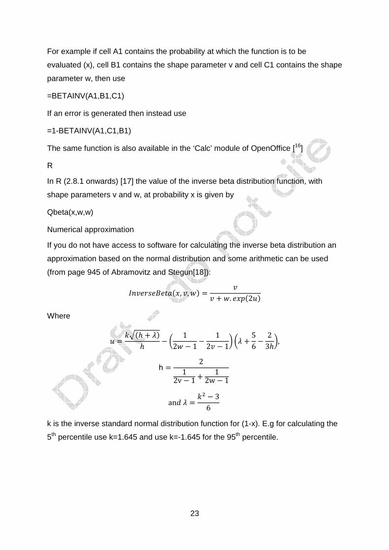
Numerical approximation

If you do not have access to software for calculating the inverse beta distribution an

approximation based on the normal distribution and some arithmetic can be used

(from page 945 of Abramovitz and Stegun[18]):

�� !� " #$��, , �� . ��2,�

Where

, � ;<�= � >�= � ? 1

2� � 1 � 12 � 1@ ?> � 5

6 � 23=@,

h � 212v � 1 � 12w � 1

anG > � ;� � 36

k is the inverse standard normal distribution function for (1-x). E.g for calculating the

5th percentile use k=1.645 and use k=-1.645 for the 95th percentile.

24

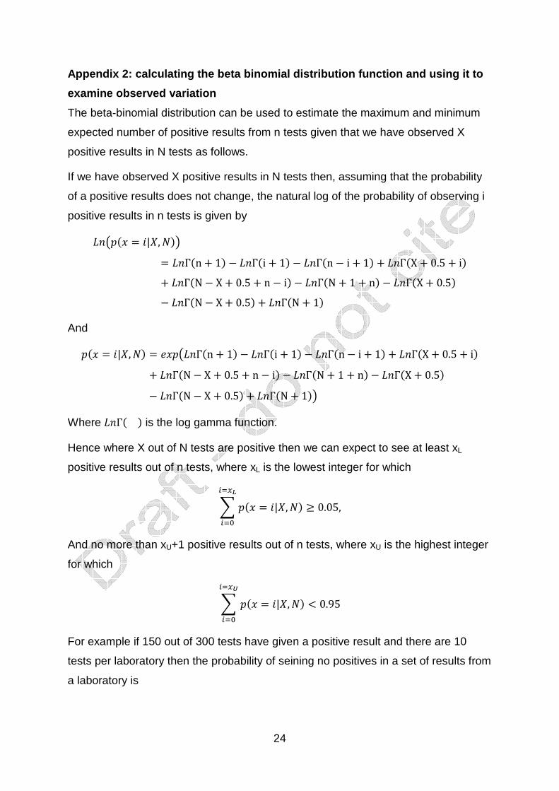
Appendix 2: calculating the beta binomial distribution function and using it to

examine observed variation

The beta-binomial distribution can be used to estimate the maximum and minimum

expected number of positive results from n tests given that we have observed X

positive results in N tests as follows.

If we have observed X positive results in N tests then, assuming that the probability

of a positive results does not change, the natural log of the probability of observing i

positive results in n tests is given by

�H�� *|�, ��J� �Γ�n � 1� � �Γ�i � 1� � �Γ�n � i � 1� � �Γ�X � 0.5 � i�� Γ�N � X � 0.5 � n � i� � �Γ�N � 1 � n� � �Γ�X � 0.5�� Γ�N � X � 0.5� � �Γ�N � 1�

And

�� *|�, �� H�Γ�n � 1� � �Γ�i � 1� � �Γ�n � i � 1� � �Γ�X � 0.5 � i�� Γ�N � X � 0.5 � n � i� � �Γ�N � 1 � n� � �Γ�X � 0.5�� Γ�N � X � 0.5� � �Γ�N � 1�J

Where �Γ� � is the log gamma function.

Hence where X out of N tests are positive then we can expect to see at least xL

positive results out of n tests, where xL is the lowest integer for which

� �� *|�, ��NO

��P 0.05,

And no more than xU+1 positive results out of n tests, where xU is the highest integer

for which

� �� *|�, ��NQ

��R 0.95

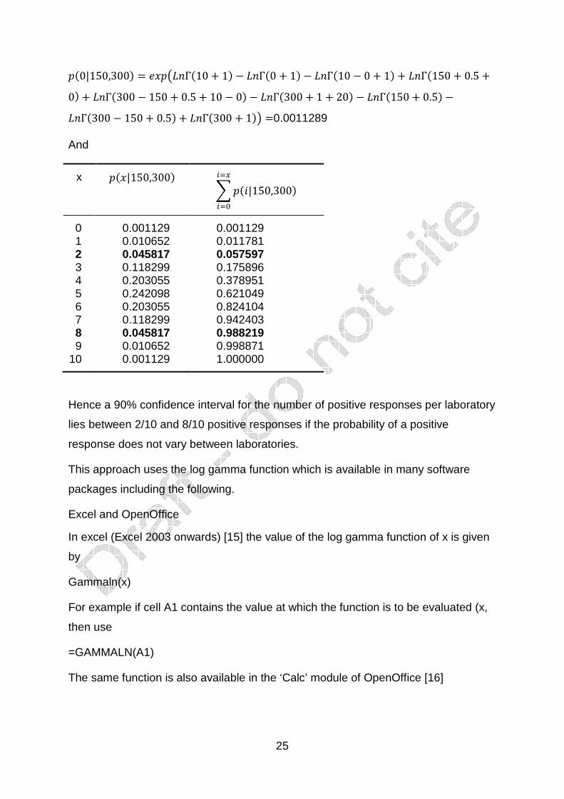
For example if 150 out of 300 tests have given a positive result and there are 10

tests per laboratory then the probability of seining no positives in a set of results from

a laboratory is

25

��0|150,300� � ��H�Γ�10 � 1� � �Γ�0 � 1� � �Γ�10 � 0 � 1� � �Γ�150 � 0.5 �0� � �Γ�300 � 150 � 0.5 � 10 � 0� � �Γ�300 � 1 � 20� � �Γ�150 � 0.5� ��Γ�300 � 150 � 0.5� � �Γ�300 � 1�J �0.0011289

And

x ��|150,300� � ��*|150,300��N

��

0 0.001129 0.001129 1 0.010652 0.011781 2 0.045817 0.057597 3 0.118299 0.175896 4 0.203055 0.378951 5 0.242098 0.621049 6 0.203055 0.824104 7 0.118299 0.942403 8 0.045817 0.988219 9 0.010652 0.998871

10 0.001129 1.000000

Hence a 90% confidence interval for the number of positive responses per laboratory

lies between 2/10 and 8/10 positive responses if the probability of a positive

response does not vary between laboratories.

This approach uses the log gamma function which is available in many software

packages including the following.

Excel and OpenOffice

In excel (Excel 2003 onwards) [15] the value of the log gamma function of x is given

by

Gammaln(x)

For example if cell A1 contains the value at which the function is to be evaluated (x,

then use

=GAMMALN(A1)

The same function is also available in the ‘Calc’ module of OpenOffice [16]

26

R

In R (2.8.1 onwards) [17] the value of the log gamma function of x is given by

lgamma(x)

References

1 Lebesi, D., Dimakou, C., Alldrick, A.J., and Oreopoulou, V.,( 2010), QAS, 2(4),

173–181

2 Horwitz, W., (1995), Pure Appl Chem 67, 331-343

3 EURACHEM (2000) Quantifying Uncertainty in Analytical Measurement, 2nd

Ed., http://www.eurachem.org/

4 Feinberg, M., Boulanger, B., Dewé, W., & Hubert, P. (2004) Anal. Bioanal.

Chem. 380, 502–514

5 Rose M, Poms R, Macarthur R, Pöpping B, Ulberth F, QAS, Accepted for

publication

6 McCullagh P, Nelder J.A., 1989, Generalized Linear Models, Second edition,

Chapman and Hall, London

7 Langton SD, Chevennement R, Nagelkeke N, Lombard B (2002) Int J Food

Microbiol, 79:171–181

8 van der Voet H, van Raamsdonk WD (2004) Int J Food Microbiol 95, 231–234

9 Wilrich C, Wilrich P-T, (2009), JAOAC Int. 92(6), 1763-1772

10 Wilrich, P-T, (2010) Accred Qual Assur (2010) 15, 439–444

11 Wehling, P., Labudde, R.A., Brunelle S.L., Nelson, M.T., (2011), JAOAC Int.,

94(1), 335-347

12 LaBudde, R.A. (2009) Coverage Accuracy for Binomial Proportion 95%

Confidence Intervals for 12 to 100 Replicates, TR297, Least Cost

Formulations, Ltd, Virginia Beach, VA,

27

http://www.lcfltd.com/Documents/tr297%20coverage%20accuracy%20binomi

al%20proportions.pdf

13 Brown L.D., Cai T.T., DasGupta A., (2001), Stat. Sci., 16(2), 101-133

14 van Hengel, A.J., Capelletti C., Brohee, M., Anklam E., (2006), JAOAC Int.

89(2), 462-468

15 Microsoft Excel online Help, http://office.microsoft.com/en-us/excel-

help/betainv-HP005209001.aspx?CTT=1

16 Open Office, http://www.OpenOffice.org

17 The R project for statistical computing, http://www.r-project.org/

18 Abramowitz, M., Stegun, I., (1972), Handbook of Mathematical Functions,

10th edition