Embed Size (px)
Citation preview

i
Rapid On-line Glycogen Measurement and Prediction of
Ultimate pH in Slaughter Beef
Dominic Lomiwes
A thesis submitted to the
Auckland University of Technology
in partial fulfilment of the requirements of the degree of
Master of Applied Science (MAppSc)
May 2008
Faculty of Health and Environmental Sciences
Primary Supervisor: Associate Professor Owen Young

ii
ATTESTATION OF AUTHORSHIP
I hereby declare that this submission is my own work and that, to the best of
my knowledge and belief, it contains no material previously published or written by
another person (except where explicitly defined in the acknowledgements), nor
material which to a substantial extent has been submitted for the award of any other
degree or diploma of a university or other institution of higher learning.
Signed: _______________________________ Date: ___________
Dominic Lomiwes

iii
ACKNOWLEDGEMENTS
I wish to acknowledge the Foundation of Research, Science and Technology for
providing some of the funding that went towards this project. I also acknowledge the
Tertiary Education Commission and AgResearch Limited for their support in granting
me a scholarship to complete this thesis.
Acknowledgements go to Dr Marlon dos Reis and to Dr John Waller for their
assistance in the statistical analyses of the data that were collected.
Thanks go to the staff of PPCS Te Aroha for welcoming us into their plant and
assisting us in the collection of data and samples for this project.
A big thank you goes to my supervisors Dr Owen Young and Dr Eva Wiklund.
Your feedback, guidance and limitless encouragement during the past year are much
appreciated.
My thanks also go to Dr Mike North, Dr Katja Rosenvold, Mr Kevin Taukiri
and the Meat Science team at AgResearch for their support in this project. Thank you
for making a place for me by taking me in as a student. You have all been so
welcoming and I have enjoyed working with you all.
Finally, thanks go to my family. Your support and encouragement has pushed
me to strive to give my best in everything that I do.

iv
CONFIDENTIAL MATERIAL
This thesis is to be examined under confidentiality, and an embargo to be placed
on library access. This work was conducted under a confidentiality agreement with
AgResearch Limited and an embargo of 18 months is to be placed on this thesis from
the time of publishing to allow AgResearch Ltd. the opportunity to protect any
intellectual property.

v
ABSTRACT
The rapid determination of glycogen on indicator muscle immediately after
slaughter is advantageous as it permits the prediction of a muscle‟s ultimate pH (pHu)
and allows the identification of high pHu meat carcasses by extrapolation. This thesis
examines the development of two rapid glycogen determination methods.
The first aim of this thesis was to find a new glucometer to replace the Bayer
ESPRIT™
(Bayer) glucometer currently used in the Rapid pH (RpH) method.
Roche‟s Accuchek® Advantage II (Accuchek) and Abbott‟s Medisense Optium
™
(Medisense) glucometers were compared. Accuchek measurements exhibited a
positive linear relationship in glucose standards made with water, RpH buffer and
glucose spiked meat/buffer slurries ranging from 0 to 500 mg dL-1
(r2 = 0.999, 0.998
and 0.995 respectively). Medisense also exhibited a strong positive relationship for
glucose standards made with water and RpH buffer; however, a non-linear trend in
spiked meat slurries was observed.
The second aim of this thesis was to explore the calibration of the KES K201
(KES Analysis Inc., NY, USA) near-infrared (NIR) diode array spectrometer to
measure glycogen and pH at approximately 45 minutes after slaughter (pH45), and to
predict pHu in pre-rigor M. longissimus dorsi (LD) from beef. This first required
finding a reference method to calibrate against the NIR instrument. The RpH, Iodine
and Bergmeyer methods were compared. Analysis of glycogen in replicate samples
of three beef LD muscles at timepoints post-mortem (1, 4, 9 and 20 hours) was
conducted. No significant difference in glycogen concentration was found between
an enzymatic and an iodine based colorimetric method at each timepoint; however,
the Iodine method was more consistent than the Bergmeyer method at all timepoints.
Glucose measurements from the RpH method were consistent; however the pattern of
glycogen decline at increasing timepoints post-mortem did not correspond with
existing published studies.
NIR spectra (538 to 1677 nm) of LD muscles from steers (n = 47), cows
(n = 28) and bulls (n = 20) routinely slaughtered in a commercial abattoir were
collected on-line approximately 45 minutes after slaughter. Poor results were
obtained for Partial Least Squares (PLS) models generated from the mean reflectance
spectra of each animal to measure glycogen and pH45, and predict pHu (r2 = 0.23, 0.37
vi
and 0.20 respectively). A high mean square error of prediction (MSEP) for glycogen
was also obtained (7.75).
Validation of qualitative models generated with Generalised Partial Least
Squares regression (GPLS) found that the optimum model was able to correctly
categorise only 42% of high pHu samples with the remaining portion being wrongly
classified as normal pHu meat. When the effect of gender was removed, only 21% of
high pHu carcasses were correctly categorised.
Exploratory analysis of the absorbance spectra of the LD muscles showed that a
group composed predominantly of steers had a significantly lower pH45 than other
existing groups. Further work is recommended for NIR to be successfully utilised on-
line to measure glycogen or predict pHu in pre-rigor carcasses.

vii
TABLE OF CONTENTS
Title Page i
Attestation of Authorship ii
Acknowledgements iii
Confidential Material iv
Abstract v
Table of Contents vii
List of Figures xi
List of Tables xiii
1 INTRODUCTION 1
2 LITERATURE REVIEW 3
NEW ZEALAND BEEF 3
INDUSTRIAL PROCESSES IN THE SLAUGHER OF CATTLE 4
Pre-slaughter handling and ante-mortem inspection 5
The slaughter of cattle 5
Electrical stimulation 6
Carcass dressing 7
Carcass boning 7
THE METABOLIC CONVERSION OF MUSCLE TO MEAT 8
The structure of muscle 9
Muscle metabolism in living animals 11
Muscle metabolism post-mortem 12
Changes in muscle structure during ageing 15
MEAT QUALITY 15
Meat colour 16

viii
Meat tenderness 18
Meat flavour 20
Pre-slaughter factors affecting meat quality 21
Post-mortem factors affecting meat quality 22
GLYCOGEN 23
The importance of glycogen for meat quality 24
The importance of determining muscle glycogen content early in the slaughter process 26
METHODS OF MUSCLE GLYCOGEN DETERMINATION 27
Isolation of glycogen from muscle 27
Alkaline extraction 27
Acid extraction 28
Hydrolysis of extracted glycogen 29
Methods of glycogen/glucose measurement 30
Colorimetric assay 30
Enzymatic assay 30
Other methods of measuring glycogen 31
Iodine method 31
Rapid pH method 32
NEAR-INFRARED SPECTROSCOPY 32
Principles of NIR 32
NIR instrumentation 33
NIR calibration and chemometrics 35
Applications of NIR spectroscopy in the Meat Industry 35
RESEARCH AND OBJECTIVES 36
Glucometer calibrations for the RpH method 36
Rapid determination glycogen in slaughter beef using NIR spectroscopy 37
3 MATERIALS AND METHODS 39
CALIBRATION OF ROCHE‟S ACCUCHEK
® ADVANTAGE II AND ABBOTT‟S
MEDISENSE OPTIUM™
FOR RAPID pH MEASUREMENT 39

ix
Chemicals, reagents and equipment 39
Glucometer response to glucose standards made with water and RpH buffer 39
Glucometer response to spiked meat slurries 40
Abattoir practice 40
On-line RpH measurement of beef samples 41
Data analysis for calibration of two new meters against the Bayer glucometer 41
COMPARISON OF THREE METHODS FOR GLYCOGEN DETERMINATION 42
Chemicals reagents and equipment 42
Sample collection and storage 42
Perchloric acid extraction of glycogen from meat 43
Iodine method for glycogen determination 43
Enzymatic method for glycogen determination 43
RpH method for glycogen determination 44
Data analysis 45
NIR CALIBRATION FOR THE QUANTITATIVE DETERMINATION OF
GLYCOGEN IN PRE-RIGOR MUSCLE 45
Chemicals, reagents and equipment 45
NIR scanning of pre-rigor samples 45
Collection and storage of muscle samples 46
Glycogen and ultimate pH measurements of NIR scanned beef samples 46
Principal Component Analysis of NIR spectra to find a representative spectrum for
each animal 47
Development of calibration models to measure glycogen and pH45 and predict pHu in
pre-rigor M. longissimus dorsi 47
Development of classification models to categorise meat into two classes of ultimate
pH 48
Exploratory analysis of NIR spectra to evaluate factors that give differences between
animal classes 49
4 RESULTS AND DISCUSSION – PART I 50
CALIBRATION OF ROCHE‟S ACCUCHEK
® ADVANTAGE II AND MEDISENSE
OPTIUM™
GLUCOMETERS FOR RAPID pH MEASUREMENT 50

x
Glucometer responses to glucose standards in water and RpH buffer 50
Glucometer responses to meat slurries spiked with glucose 51
Comparison of three glucometers in on-line RpH measurement of beef carcasses in a
commercial abattoir 53
Choice of a replacement meter for the Bayer glucometer 55
5 RESULTS AND DISCUSSION – PART II 62
COMPARISON OF THREE GLYCOGEN DETERMINATION METHODS 62
Determination of glycogen in M. longissimus dorsi 62
Final choice of glycogen reference method for NIR calibration 64
NEAR-INFRARED SPECTROPSCOPY 66
Near-infrared scanning of muscle and selection of scans for data analysis 66
Development of calibration models to measure the glycogen concentration and pH45
and predict pHu in pre-rigor muscle 69
Development of classification models to categorise meat into two classes pHu 75
Exploratory analysis to NIR spectra to evaluate factors that give differences between
genders 79
Discussion 84
6 CONCLUSIONS AND RECOMMENDATIONS 89
CONCLUSIONS 89
RECOMMENDATIONS FOR FURTHER RESEARCH 90
REFERENCES 91

xi
LIST OF FIGURES
Figure 1 A diagram of a skeletal muscle fibre. They are unbranched, arranged
longitudinally and bound by sarcolemmas.
10
Figure 2 Diagram of a skeletal muscle and its constituents. 10
Figure 3 Diagrammatic representation of a sarcomere at various stages of contraction. 11
Figure 4 A schematic diagram of the glycolytic pathway and tricarboxylic acid cycle
(TCA).
14
Figure 5 Kinetics of glycogen loss, pH fall and lactate accumulation in longissimus
lumborum muscle from an unstimulated bovine carcass.
14
Figure 6 The myoglobin molecule consists of a helical polypeptide chain and a haem
group within the folded chain. The different forms of the myoglobin
molecule are also shown.
17
Figure 7 The colour of meat at various pH levels. 17
Figure 8 An example of muscle shortening. 19
Figure 9 The relationship of ultimate pH (pHu) to the concentration of glycogen
present in muscle at death.
25
Figure 10 A diagram of a diode-array detector. 34
Figure 11 On-line collection of NIR spectra from a beef carcass. 46
Figure 12 Glucometer readings of a range of glucose concentrations in water and Rapid
pH (RpH) buffer.
52
Figure 13 Glucometer readings from spiked postrigor meat slurries in RpH buffer and
amyloglucosidase.
54
Figure 14 Plots of three glucometer readings from individual animals as a function of
the mean of the three glucometer readings from each animal muscle slurry.
56
Figure 15 Accuchek glucometer readings as a function of Bayer glucometer readings
for each of the 45 muscle slurries.
56

xii
Figure 16 Medisense glucometer readings as a function of Bayer glucometer readings
for each of 45 muscle slurries.
57
Figure 17 Mean glycogen values of longissimus dorsi muscle samples and their
corresponding standard deviations at different time points post-mortem.
63
Figure 18 A typical plot showing the 20 near-infrared spectra collected from prerigor
longissimus dorsi muscle of one animal.
67
Figure 19 Principal Component Analysis of near-infrared spectra showing the 10
selected spectra.
68
Figure 20 Mean Square Error of Prediction (MSEP) and coefficient of determination
(r2) values of Partial Least Squares (PLS) models of the reflectance spectra
(538 to 1677 nm) for the prediction of glycogen in pre-rigor muscle.
71
Figure 21 Mean Square Error of Prediction (MSEP) and coefficient of determination
(r2) values of Partial Least Squares (PLS) models of the reflectance spectra
(538 to 1677 nm) for the prediction of ultimate pH (pHu) in pre-rigor muscle.
73
Figure 22 Mean Square Error of Prediction (MSEP) and coefficient of determination
(r2) values of Partial Least Squares (PLS) models of the reflectance spectra
(538 to 1677 nm) for the prediction of pH45 in pre-rigor muscle.
74
Figure 23 Calibration model and validation of classification models with gender effect
taken into account. Classification was based on the probability of samples
reaching an ultimate pH (pHu) lower than 5.7.
76
Figure 24 Calibration model and validation of classification models after the
subtraction of gender effect.
77
Figure 25 Illustration of the exploratory analysis of a small data set (seven samples
described by two variables).
80
Figure 26 Hierarchical Cluster Analysis of the absorbance spectra (538-1677 nm) of
pre-rigor LD muscle from 96 animals.
82
Figure 27 Average of reference values for similar groups that have been identified after
Hierarchical Cluster Analysis of the absorbance spectra of 96 animals.
83

xiii
LIST OF TABLES
Table 1 Percent variances of glycogen concentration in longissimus dorsi muscle
samples at different timepoints post-mortem as measured by three methods.
64
Table 2 Summary of results for PLS models fitted to predict glycogen, pHu and
pH45 in pre-rigor LD muscle by leave-out-one cross validation.
70
Table 3 Percentage of correct and incorrect classification of calibration and
validation data for GPLS classification models with the inclusion and
exclusion of gender effects.
78

Chapter 1 Introduction
1
CHAPTER 1
INTRODUCTION
The rapid glycogen determination of pre-rigor muscle of freshly slaughtered
beef carcasses is important in the prediction of ultimate pH (pHu). Many quality
attributes are dependent on the meat‟s pHu and meat with the most desirable
properties generally have „normal‟ pHu values ranging from 5.4 to 5.6. In some meat
processing plants, meat with an elevated ultimate pHu of 5.7 to 6.1 and greater than
6.1 are classed as intermediate pHu and high pHu, respectively. Meat with an elevated
pHu is undesirable as a table cut because it is dark in colour, inferior in flavour and
highly susceptible to microbial degradation. For this reason, they meat is usually sold
at a lower price than normal pHu meat.
For muscle to achieve normal pHu, it must contain sufficient concentration of
glycogen at the time of slaughter. When the muscle undergoes anaerobic metabolism
after slaughter, glycogen is converted to lactic acid via the glycolytic pathway. Lactic
acid accumulates in the meat causing the meat pH to fall. If the glycogen
concentration is limited, pH decline is arrested at higher values, frequently resulting in
DFD meat.
The New Zealand pastoral production system generates a range of meat pHu
values. Approximately 70 percent of bulls, 30 percent of cows and 10 percent of
steers yield beef with high pHu values (pHu > 5.8). Due to this high production of
high pHu beef, most beef produced from bulls and cows is sold as frozen
manufacturing commodities at a lower price than beef from steers. In contrast, prime
beef (from steers) are sold as higher value chilled products. This approach leads to
loss in profitability as a significant amount of cows and bulls will yield meat with a
normal pHu that could be sold as higher value chilled products. Conversely, there are
instances where chilled beef designated as „prime‟, is actually high pHu meat, which
leads to customer dissatisfaction.
For processors to optimise profitability from their product, a method of rapidly
identifying carcasses that will yield high pHu meat is required before carcasses are hot
boned and packed. A significant curvilinear relationship exists between the pHu of

Chapter 1 Introduction
2
beef and the glycogen content immediately after slaughter. This means that it is
possible to predict the pHu of muscle if the glycogen content after slaughter is known.
Developments in two on-line methods of rapidly measuring glycogen in pre-
rigor beef muscle are examined in this thesis. The recent discontinuation in
production of Bayer glucometers used for the existing Rapid pH (RpH) method has
seen the need for the calibration of a new glucometer to replace the Bayer model. The
efficacy of near-infrared (NIR) spectroscopy as an on-line instrument to rapidly
measure glycogen in pre-rigor beef was also investigated. Although previous studies
have shown NIR as a spectroscopic tool capable of measuring several meat quality
attributes, its applicability as an on-line tool in commercial abattoirs is largely
unknown. Thus, this thesis explores the efficacy of NIR spectroscopy as an on-line
instrument to rapidly measure glycogen in pre-rigor beef muscle.
Chapter 3 of this thesis details the materials and methods that were used. This is
followed by the presentation of the results and discussions in Chapters 4 and 5 where
results obtained on finding a replacement glucometer for the RpH method are
presented. Finally, the calibration and success of NIR spectroscopy to quantify
glycogen and predict the pHu of pre-rigor beef muscle is discussed.
Conclusions drawn from the results are presented in Chapter 6.
Recommendations for further research with regards to the rapid determination of
glycogen using NIR spectroscopy are also discussed.

Chapter 2 Literature Review
3
CHAPTER 2
LITERATURE REVIEW
NEW ZEALAND BEEF
The agricultural sector is a significant revenue earner to the New Zealand
economy and makes up 6% of the global meat trade ("Meat and Wool New Zealand,"
2007a). In the year ended March 2007, over 360,000 tonnes of beef were exported
earning over $1.8 billion, which is up 5% on the previous year (MAF, 2007).
Cattle, which are all eventually destined for beef production in one form or
another, are predominantly raised in the North Island, accounting for 75 percent of the
4.4 million cattle in New Zealand (Meat and Wool New Zealand, 2007a).
Approximately half of the meat produced from cattle is from steers (male castrates)
and heifers (virgin females), collectively classified as prime, with cows and bulls
making up most of the remaining half (Statistics New Zealand, 2007). Beef cattle
come from a variety of breeds but mainly from Angus, Hereford, Angus Hereford
and Friesian lines.
Up to 80% of beef produced in New Zealand is exported. New Zealand‟s
largest beef market is the United States taking about 50 percent of all New Zealand
beef exports. Most of this beef is frozen manufacturing grade beef from cows and
bulls. North Asia (Japan, South Korea and Taiwan) is the second largest market with
23% of beef produced in 2006 exported to these countries ("Meat and Wool New
Zealand," 2007b). Other major international markets are South Asia and the Pacific
nations.
New Zealand cattle are overwhelmingly pasture-fed, which is a key factor that is
used to differentiate New Zealand beef from many competitors. This is particularly
important in the United States where beef cattle are cereals-finished resulting in meat
with a high intramuscular fat content (marbling) compared with meat from New
Zealand. The difference between the beef produced from both countries is
complementary as they are destined for different food purposes. In the United States,
locally produced beef are destined as higher value cuts whereas beef imported from

Chapter 2 Literature Review
4
New Zealand are intended for manufacturing purposes. This is the driver for New
Zealand‟s strong export trade with the United States.
The success of New Zealand beef exports is also due to the marketing of New
Zealand beef in North Asia. Consistent emphasis is placed on New Zealand beef
cattle as being raised in a „natural‟ free-range environment and claims that New
Zealand beef is a healthier food alternative to grain-finished beef. Emphasis is also
placed in New Zealand beef as a safe, disease-free product. This is particularly
important in the North Asian market where bovine spongiform encephalopathy (BSE)
was detected in American and Canadian beef in 2003. This led to the immediate ban
of North American beef exports between 2003 and 2006 leaving New Zealand and
Australia as the only countries allowed to export beef to Japan and South Korea in
that period (MAF, 2007). In these years, New Zealand‟s beef market share in Japan
quadrupled from 2.1 to 8.5 percent (Meat and Wool New Zealand, 2007b).
Although international prices for New Zealand beef are currently at an all time
high with beef production forecast to increase within the next two years (MAF, 2007),
there are challenges that face the beef industry. The increase in the proportions and
absolute numbers of discerning consumers in key markets has seen increased
emphasis placed on safety, quality and convenience on products that must also be
competitively priced. Innovative research is critical to meet these demands where
new technologies can be applied to cut costs, add value or to ensure that consistent
high quality is achieved.
INDUSTRIAL PROCESSES IN THE SLAUGHTER OF CATTLE
In order to understand the different factors affecting meat quality, it is important
to have an overview of processes involved in the slaughter of animals and the general
handling of the carcass. In New Zealand, strict guidelines dictating the slaughter
process and handling of the carcass revolves around animal welfare and hygiene.
Although exact slaughter processes vary between abattoirs, the method of slaughter
and the subsequent treatment of the carcass are relatively similar.

Chapter 2 Literature Review
5
Pre-slaughter handling and ante-mortem inspection
Animals scheduled for slaughter are held in lairage before slaughter. This
allows animals to be easily directed into laneways that lead to the slaughter line.
Ideally, animals are kept in unmixed groups to avoid undue stress and injuries that
they may acquire from social interaction and fighting with unfamiliar animals.
However, in an abattoir situation, this may not always be the case.
Antemortem examinations of animals are conducted prior to slaughter. At this
stage, animals are individually observed for signs of transmittable diseases or stress
that may produce meat unacceptable for human consumption. After an animal has
passed the inspection, it is cleared for slaughter. Animals that exhibit signs of
sicknesses or other abnormalities are inspected further.
The slaughter of cattle
Stunning is the first step in the slaughter process. The stunning of an animal is
performed to fulfil humane slaughter guidelines that require the animal to be
“rendered insensible to pain prior to being slaughtered by bleeding” (NZFSA, 2002).
There are many methods used to achieve insensibility. In New Zealand, electrical
stunning of cattle is predominantly employed.
Head-only electrical stunning is the most common method of stunning in New
Zealand. It works by passing a current through the animal‟s brain. The current
applied results in an epileptic reaction in the animal where all parts of its brain are
stimulated. This results in the induced unconsciousness and insensibility of the
animal. In a typical stunning system, the current is passed through electrodes behind
the ears and on the nose of the restrained animal. The insensible and relatively
motionless animal is then presented for slaughter.
Sticking is the generic term used to describe the severing of the vessels
supplying blood to the brain. Once sticking has been performed, the animal is
exsanguinated quickly, ultimately leading to the animal‟s death. In New Zealand, two
methods of sticking are used. These are thoracic stick and the halal stick.
In a thoracic stick, an incision is made in the chest of the animal towards the
heart where the branchiocephalic trunk is severed using a knife. The
branchiocephalic trunk gives rise to carotid arteries that supply blood to the brain.
Once the stunned animal has been shackled on a hind leg and hoisted, the stick is then

Chapter 2 Literature Review
6
performed on the thoracic inlet between the first and the second rib of the suspended
animal. This results in rapid exsanguination.
A halal stick is made by an incision in the neck with a knife severing the carotid
arteries and jugular veins, similarly resulting in exsanguination and death (Shragge &
Price, 2004). There are several requirements for the halal slaughter of animals. In
New Zealand, for an abattoir to be halal certified, the person conducting the halal
stick must be Muslim. The name of Allah (God) must be spoken over the animal and
stick must be carried out from the front (chest) of the animal and not from the back. It
is required that the death of the animal results from the stick and subsequent
exsanguination. It is for this reason that electrical stunning is used only to immobilise
animals before slaughter. While electrical stunning induces unconsciousness and
insensibility to animals, it does not kill the animal, and given a few minutes, the
animal can fully recover and live a normal life (Shragge & Price, 2004).
Most cattle in New Zealand are slaughtered according to halal procedures. The
halal slaughter of beef cattle is currently an issue in New Zealand. Beef imports from
New Zealand to Malaysia were banned in 2005 after inspectors decided that halal
procedures were not fully adhered to (NZPA, 2007). By complying with halal
procedures, export meat is accessible by both the Muslim and non-Muslim
communities since the latter have no religious requirements.
Electrical stimulation
The application of low voltage electrical stimulation to a carcass is commonly
applied following exsanguination and death. Low voltage electrical stimulation is
achieved by passing a current through a freshly slaughtered carcass where the current
is applied through the shackled left hind hoof and passes out through an electrode
manually clipped on the nose, head or neck of the carcass (Devine, Hopkins, Hwang,
Ferguson, & Richards, 2004). The application of an electric current causes the
muscles in the carcass to contract increasing the metabolic breakdown of glycogen
and a rapid fall of pH. This has implications in meat quality where the toughness in
meat resulting from a phenomenon known as cold shortening is reduced (Hwang,
Devine, & Hopkins, 2003). This is further discussed later in this chapter in the
MEAT QUALITY section.

Chapter 2 Literature Review
7
Carcass dressing
The dressing of a carcass is carried out from an overhead rail system that
continues the production line from the point of stunning. Over the past decades, the
Zealand meat industry has invested heavily in the mechanisation of the dressing
process to replace as many labour units as possible and to increase process efficiency.
After electrical stimulation, the hooves and head are first removed and the
carcass is prepared for hide stripping. This is achieved using capstans which pull the
hide downward to separate it from the subcutaneous muscles (Belk & Scanga, 2004).
Two operators stand on motorised descending platforms at each side of the carcass
and assist with hide removal using rotating shears (Longdell, 2000).
The evisceration of the carcass then follows where the abdomen is split open
and the viscera (rumen, intestines, liver and spleen) are removed along with other
internal organs. Some organs such as the heart and liver undergo inspection to
determine any abnormalities that may result in the carcass being condemned (Belk &
Scanga, 2004).
Following evisceration, the carcass is halved by sawing it longitudinally from
tail to neck along the vertebral column. It is then quartered between the 12th and 13th
ribs but cutting only through the vertebrae so that the carcass remains as two sides
rather than four pieces. It then progresses to a grading station where the final
inspection for any abnormalities is made and a grade assigned based on weight,
fatness, gender, and other factors depending on the abattoir‟s target market. After
passing the final inspection, the sides are then either moved to a chiller or
immediately hot boned.
Carcass boning
After dressing, the carcass sides are traditionally held in a chiller set between 2
to 4°C for approximately 36 hours before it is boned into commercial cuts (Ockerman
& Basu, 2004). This method is known as cold boning because the carcass had
reached the chiller temperature and rigor mortis is complete during boning (Waylan &
Kastner, 2004). In meat processing plants, cold boning is normally carried out on
prime animals destined for export or animals destined for local consumption.
Alternatively, whole carcasses are also transported in refrigerated trucks to local meat

Chapter 2 Literature Review
8
retailers where the meat may be aged before it is boned and sold as table cuts by the
retailer.
Hot boning is the removal of lean meat and fat from the carcass preceding rigor
mortis. Most hot boned beef processed in New Zealand is exported frozen in plastic-
lined cartons for manufacturing purposes. In contrast to cold boning, hot boning is
carried out while the carcass is still warm, and in New Zealand, this happens
immediately after the grading point, typically within 45 minutes after slaughter. High
value cuts such as striploins (M. longissimus dorsi) and tenderloins (M. psoas major
and minor) are removed, vacuum packed and chilled. The rest of the carcass is boxed
and blast frozen. Hot boned meat from cows and bulls are immediately frozen after
boning as the enduring market perception is that muscles from these animals will
yield meat that is of inferior eating quality.
There are many advantages to hot boning over the conventional cold boning
practice. Hot boning is estimated to save meat processors up to 50 percent of
refrigeration costs and space. Other advantages of hot boning are labour savings,
shorter processing times and lower transport costs of the product (Ockerman & Basu,
2004).
Although hot boning brings many advantages, concerns regarding its effect on
meat quality have been raised. These concerns include the higher microbial
susceptibility of hot boned meat (Taylor, 1995). As hot boning is conducted at higher
temperatures than the conventional cold boning method, there is a higher risk of
bacterial growth on the meat. Although there may be conflicting views on this matter,
research has found that hot boned meat are microbiologically equivalent to cold boned
meat (Bell, Harrison, Moorhead, & Jones, 1998; Waylan & Kastner, 2004) as long as
prescribed hygiene practices are followed. Additional concerns with the hot boning
method are the retention of muscle shape and the increased incidence of
shortening/toughening of the meat that can occur because, unlike the cold boning
method, the muscles are not restrained by the skeleton until rigor mortis is reached.
THE METABOLIC CONVERSION OF MUSCLE TO MEAT
Immediately after slaughter, the transport of nutrients and oxygen to within the
body of the animal is stopped due to the massive loss of blood. This leads to changes

Chapter 2 Literature Review
9
in the metabolic processes within the animal, where aerobic metabolism stops and
anaerobic metabolism takes over. This has implications to the biochemistry and
structure of the muscle as it enters the rigor mortis state to become meat as we know
it.
The structure of muscles
Meat is heterogeneous and is macroscopically composed of contractile tissue
(true muscle), fat, and connective tissue. Skeletal muscle generally represents a bulk
(35 to 65 percent) of the carcass weight of slaughtered animals. Meat also contains
some smooth muscle as a component of blood vessels (Hendrick, Aberle, Forrest,
Judge, & Merkel, 1994). Due to people‟s concept of meat and muscle, the two terms
are sometimes used interchangeably. In this thesis, the term meat is used to describe
muscle that is in rigor.
Skeletal muscle is made up of structural units called muscle fibres (cells) which
are bound together into muscle bundles and are in turn collectively grouped to make
the muscle. Muscle fibres make up 75 to 92 percent of the total muscle volume, with
connective tissues, blood vessels and extracellular fluid accounting for the remaining
volume (Hendrick et al., 1994).
Skeletal muscle fibres from mammals are long, threadlike cells with tapered
ends (Figure 1). Although they may reach lengths of up to several centimetres long,
these unbranched cells usually do not extend the length of the muscle. Muscle fibres
contain all the organelles normally found in living cells within their sarcoplasm
(cytoplasm) and are bound by a collagen-stabilised membrane known as a
sarcolemma. Sarcolemmas have elastic properties, which allows them to endure
considerable distortion during muscle contraction, relaxation and stretching (Hendrick
et al., 1994).
A breakdown of skeletal muscle and its components are shown in Figure 2.
Muscle fibres are unique in that within the sarcoplasm, there is a regular arrangement
of cylindrical myofibrils lying side by side and oriented longitudinally along the entire
length of the cell. Each myofibril is made up of smaller components known as
myofilaments, dominantly comprising of so-called thick and thin filaments. Thick
filaments are composed of the multichained protein myosin. Thick filaments are
organised longitudinally in exact alignment parallel to each other across the myofibril.
Thin filaments, which are made up of actin proteins are also aligned parallel to each

Chapter 2 Literature Review
10
other across the myofibril and are arranged between two sections of thick filaments.
This alternating arrangement of the myofilaments shows up as transverse bands along
the skeletal muscle when observed microscopically. It is for this reason why skeletal
muscle is also referred to as striated muscle (Hendrick et al., 1994).
Myofibrils
NucleiConnective
tissue
Tapered end of
the fibreSarcolemmaMyofibrils
NucleiConnective
tissue
Tapered end of
the fibreSarcolemma
Figure 1: A diagram of a skeletal muscle fibre (Hendrick et al., 1994). They are
unbranched, arranged longitudinally and bound by sarcolemmas. The fibres do
not extend the length of the cell and have tapered ends.
Actin
MyosinZ Lines
Actin
MyosinZ Lines
Figure 2: Diagram of a skeletal muscle and its constituents (Hendrick et
al., 1994). Myofibrils are predominantly composed of myosin (thick
filaments) and actin (thin filaments).

Chapter 2 Literature Review
11
Muscle metabolism in living animals
Muscles cells are developed to convert chemical energy into mechanical energy.
Myofilaments are important as they are involved in the contraction and relaxation of
the muscle in a mechanism known as the sliding filament hypothesis (Huxley, 1969).
During muscle contraction, the thick and thin filaments slide over one another and
become linked by cross bridges formed between actin and myosin proteins (Figure 3).
When they are in this state, their combined configuration is referred to as actomyosin
(Warriss, 2000).
Energy is required to achieve the work of muscle contraction. The energy is
dominantly derived from the nucleotide adenosine triphosphate (ATP) produced by
enzyme systems in the sarcoplasm and mitochondria of the muscle fibres1. Energy
production from ATP needed to fuel muscle contraction is catalysed by a calcium
ATPase where ATP is hydrolysed to adenosine diphosphate (ADP) and inorganic
phosphate. The enzyme system (ATPase) that regulates this reaction is located in the
head of the myosin molecule, whose activity is triggered by the release of calcium
ions (Ca2+
) in the sarcoplasm2. The hydrolysis of ATP and the resulting contraction of
the muscle due to the cross bridges formed between actin and myosin proteins convert
chemical energy into mechanical energy (Hendrick et al., 1994). ATP is also
involved in actomyosin dissociation resulting in muscle relaxation (Davies, 2004).
Figure 3: Diagrammatic representation of a sarcomere at
various stages of contraction (Hendrick et al., 1994).
In the muscle of living animals, fuel for the production of ATP is mainly
sourced from carbohydrates in the blood (mainly glucose), free fatty acids, or
glycogen. These substrates undergo aerobic metabolism. In unstressed animals,
1 Creatine phosphate provides some energy.
2 In this sense myosin is an enzyme, but it is usually referred to as a structural protein of muscle.
Stretched muscle
(at rest)Contracted muscle
Stretched muscle
(at rest)Contracted muscle

Chapter 2 Literature Review
12
glucose is metabolised for ATP production and surplus energy is stored as glycogen
and creatine phosphate in the muscle cells. The production of ATP from glucose
sequentially involves glycolysis, oxidative decarboxylation and oxidative
phosphorylation. On the whole, the production of ATP is a complex process but only
a brief outline is needed for the scope of this thesis.
Glucose in the blood initially undergoes glycolysis where it is broken down to
give two molecules of pyruvate3 (Figure 4). During glycolysis, two ATP molecules
are consumed and four ATP molecules are generated from adenosine diphosphate
(ADP) and phosphate. Thus a net yield of two ATP molecules and four hydrogen
atoms are gained for each glucose molecule converted to pyruvate.
The two pyruvate molecules formed from the glycolysis of glucose then
undergoes decarboxylation. A CO2 molecule is initially lost from pyruvate resulting
in the formation of acetyl coenzyme A (acetyl-CoA). Decarboxylation occurs in a
cycle known as Krebs or tricarboxylic acid (TCA) cycle. During this cycle, pyruvate
loses carbon as CO2 and in the process generate hydrogen atoms carried as nicotine
adenine dinucleotide (NADH) or flavin adenine dinucleotide (FADH2). Ten
hydrogen atoms are generated from each pyruvic acid. Thus a net yield of 20
hydrogen atoms is gained from the decarboxylation of two pyruvate molecules.
The final phase of ATP production from the metabolism of carbohydrate in
muscle is oxidative phosphorylation. Up to this point, a net yield of 24 hydrogen
atoms has been generated from the glycolysis of glucose and oxidative
decarboxylation of the pyruvate molecules in the TCA cycle. Oxidative
phosphorylation occurs in the cytochrome system where a pair of hydrogens enters
the system as NADH. For each two hydrogen, three molecules of ATP are generated.
Thus, 36 ATP molecules are generated from the metabolism of one glucose molecule
in addition to the ATP generated from glycolysis (Warriss, 2000).
Muscle metabolism post-mortem
Muscles do not immediately stop functioning following the death of an animal
as metabolic enzymes controlling glycolysis and ATP production are still active
(Hamm, 1977). However, the activities of these metabolic enzymes are variously lost
within a few hours or days post-mortem due to the cessation of the circulatory system
3 Or more accurately, a mix of pyruvic acid and pyruvate depending on the pH in muscle cells.

Chapter 2 Literature Review
13
which transports oxygen and glucose to the muscle. In the absence of oxygen,
pyruvate can no longer be metabolised via the aerobic TCA cycle, thus it is
anaerobically metabolised to lactic acid. Although much less ATP is produced from
the anaerobic metabolism of glucose than by the complete process to CO2 and water,
it is enough to retain muscle extensibility for some hours. Generation of ATP is an
attempt to maintain the ATP concentrations to preserve muscle homeostasis
(Hendrick et al., 1994).
One significant post-mortem change in muscle due to anaerobic metabolism is
the lowering in the pH of the muscle. During anaerobic metabolism, muscles
preferentially utilise glycogen over free glucose remaining in the muscle. This is
perhaps because glucose has to come in the muscle via the blood stream which is no
longer functioning. Glycogen, however, is in situ. Another proposed reason for the
preferential utilisation of glycogen over glucose for anaerobic metabolism is that the
phosphorylation of glycogen-derived glucose does not require ATP as does
hexokinase-catalysed phosphorylation of glucose. Hence, glycogen derived glucose
is more energy efficient. The generation of ATP through the anaerobic metabolism of
glycogen results in lactic acid as the terminal metabolite (Figure 4). In live animals,
any excess production of lactic acid due to temporary oxygen deprivation is
transported via the circulatory system away from the muscle (Hendrick et al., 1994).
However, in carcasses where the circulatory system has been terminated, lactic acid
necessarily accumulates in the muscle. Glycolysis usually ceases before all glycogen
has been used up. This may be explained by the inactivation of glycolytic enzyme
systems due to the low pH that develops within the muscle. In a well-fed, unstressed
animal the pH fall is typically from 7.2 to an ultimate pH of 5.5 (Warriss, 2000).
ATP is essential in keeping muscle in a relaxed state by preventing the
formation of actomyosin (Warriss, 2000). Muscle shows extensible properties while
ATP is still abundant in the carcass. However, as the pH decreases and the
metabolism of glycogen is halted, ATP concentrations finally fall below a threshold
required to maintain relaxation in muscles (Greaser, 2001). When this occurs, actin
and myosin combine to form permanent cross bridges resulting in rigor mortis where
the muscle tends to shorten and, as the name rigor suggests, extensibility is lost
(Marsh & Carse, 1974). The anaerobic depletion of glycogen and ATP are observed
within a few hours post-mortem. The kinetics of the fall in glycogen concentration,
decrease in pH and increase in lactate are illustrated in Figure 5.

Chapter 2 Literature Review
14
Figure 4: A schematic diagram of the glycolytic pathway and tricarboxylic acid
cycle (TCA). During aerobic metabolism, pyruvic acid is converted to acetyl-CoA
which enters the TCA cycle. However, in the absence of oxygen, pyruvic acid is
converted to lactic acid as the terminal metabolite.
Figure 5: Kinetics of glycogen loss, pH fall and lactate accumulation in longissimus
lumborum muscle from an unstimulated bovine carcass (Young, West, Hart, &
Otterdijk, 2004).
Citric acid
Isocitric acid
a-ketoglutarate
Succinyl-CoA
Succinic acid
Fumaric acid
Malic acid
Oxaloacetic acid
Tricarboxylic Acid Cycle
Fructose-1,6-
phosphate
Glyceraldehyde-3-
phosphate
Glucose
Glucose-6-
phosphate
Glycerol-1,3-phosphate
1,3-diphosphoglyceric
acid
3-phosphoglyceric
acid
Phosphoenol
pyruvic acid
PyruvateGlycogen
Glucose -1-
phosphate
anaerobic aerobic
Lactic acid Acetyl-CoA
Glycolytic Pathway
Time after slaughter, hours
0 5 10 15 20 25
Gly
co
ge
n, m
g/g
2
4
6
8
10
12
14
16
18
pH
5.0
5.5
6.0
6.5
7.0
La
cta
te c
on
cn
.,
mo
le/g
10
30
50
70
90
110
pH
Glycogen
Lactate
Chapter 2 Literature Review
15
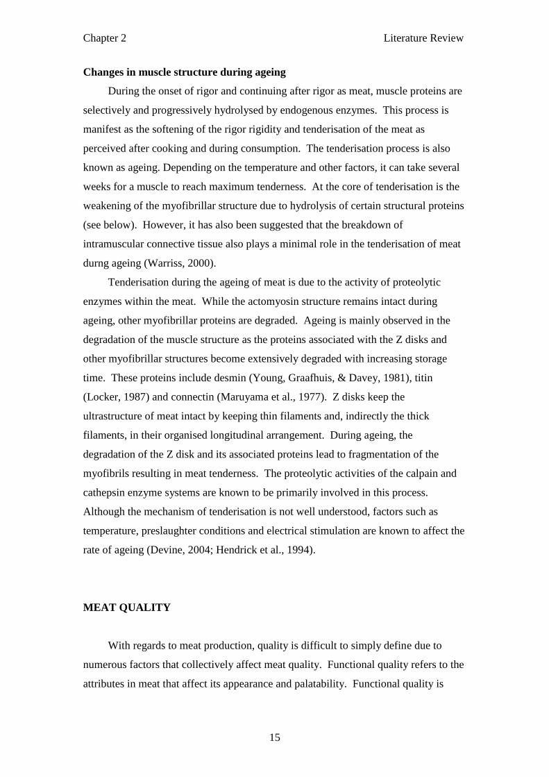
Changes in muscle structure during ageing
During the onset of rigor and continuing after rigor as meat, muscle proteins are
selectively and progressively hydrolysed by endogenous enzymes. This process is
manifest as the softening of the rigor rigidity and tenderisation of the meat as
perceived after cooking and during consumption. The tenderisation process is also
known as ageing. Depending on the temperature and other factors, it can take several
weeks for a muscle to reach maximum tenderness. At the core of tenderisation is the
weakening of the myofibrillar structure due to hydrolysis of certain structural proteins
(see below). However, it has also been suggested that the breakdown of
intramuscular connective tissue also plays a minimal role in the tenderisation of meat
durng ageing (Warriss, 2000).
Tenderisation during the ageing of meat is due to the activity of proteolytic
enzymes within the meat. While the actomyosin structure remains intact during
ageing, other myofibrillar proteins are degraded. Ageing is mainly observed in the
degradation of the muscle structure as the proteins associated with the Z disks and
other myofibrillar structures become extensively degraded with increasing storage
time. These proteins include desmin (Young, Graafhuis, & Davey, 1981), titin
(Locker, 1987) and connectin (Maruyama et al., 1977). Z disks keep the
ultrastructure of meat intact by keeping thin filaments and, indirectly the thick
filaments, in their organised longitudinal arrangement. During ageing, the
degradation of the Z disk and its associated proteins lead to fragmentation of the
myofibrils resulting in meat tenderness. The proteolytic activities of the calpain and
cathepsin enzyme systems are known to be primarily involved in this process.
Although the mechanism of tenderisation is not well understood, factors such as
temperature, preslaughter conditions and electrical stimulation are known to affect the
rate of ageing (Devine, 2004; Hendrick et al., 1994).
MEAT QUALITY
With regards to meat production, quality is difficult to simply define due to
numerous factors that collectively affect meat quality. Functional quality refers to the
attributes in meat that affect its appearance and palatability. Functional quality is

Chapter 2 Literature Review
16
addressed in this section as consumers usually refer to functional quality attributes
when discussing meat quality.
The three dominant attributes by which consumers judge meat quality are
appearance, texture and flavour (Faustman & Cassens, 1990), all of which are sensory
properties. The conformance of these attributes to consumer‟s expectations is
important and deviating from this will affect the product‟s marketability. In this
section, meat colour, tenderness and flavour are addressed. Their importance to meat
quality and factors affecting these attributes are discussed in this section.
Meat colour
The colour of lean meat is critical to the consumer‟s purchase decision as it is
often the only criterion by which a consumer can judge meat quality (Warriss, 2000).
In raw lean beef, a bright cherry red colour is most ideal as consumers perceive this as
an indicator of a fresh, good quality meat. Meat colour is also linked to other meat
quality attributes. Tests conducted on a sensory panel have found that lean colour is
significantly related to the panel‟s tenderness and flavour intensity scores (Viljoen,
Kock, & Webb, 2002).
Myoglobin is the protein largely responsible for the pigmentation of meat
(Figure 6). Meat colour is determined by the proportions of the three forms
myoglobin present in the meat (Tang et al., 2005). Myoglobin is a molecule with a
protein portion (globin) and a non-protein portion known as a haeme ring. Within the
haeme ring is an iron atom. The oxidation state of this atom governs the colour of
meat (Hendrick et al., 1994).
The development of colour in meat is known as blooming. In uncut meat, which
is unexposed to the oxygen in air, myoglobin exists in its reduced ferrous state (Fe2+
)
with no bound oxygen Meat in this state is purple-red. This form of myoglobin is
known as deoxymyoglobin. However, when the meat is exposed to air, through size
reduction by cutting for example, deoxymyoglobin reacts with oxygen to form a
pigment called oxymyoglobin. This red pigment is responsible for the desirable
bright colour in meat.

Chapter 2 Literature Review
17
Figure 6: The myoglobin molecule (left) consists of a helical polypeptide chain and a
haem group within the folded chain (Garret & Grisham, 2005). The different forms of
the myoglobin molecule are shown (right). The colour of meat is regulated by the
oxidation state of iron in the haem group within the molecule.
For chemical reasons beyond the scope of this review, at low but not zero
concentrations of oxygen, oxymyoglobin tends to undergo oxidation (where the Fe2+
in the haem is oxidised to Fe3+
) to form the undesirable brown pigment metmyoglobin
in meat. This problem is particularly prominent in vacuum-packed meat where low
concentrations of air can permeate through the packaging and accelerate
metmyoglobin formation (Hendrick et al., 1994). Metmyoglobin can be
enzymatically reduced back to oxymyoglobin. However, once meat has undergone
conditioning, residual enzymatic activity within the meat has declined and reducing
equivalents are lost, metmyoglobin reduction does not occur and the meat remains
discoloured (O'Keeffe & Hood, 1982).
Figure 7: The colour of meat at various pH levels (MIRINZ Food Technology and
Research, 1999). With the upper control threshold for the ultimate pH at 5.8, meat
with an ultimate pH equal or greater than this is classified as dry, firm and dark
(DFD).

Chapter 2 Literature Review
18
The effect of ultimate pH on the colour of meat is widely known (Figure 7).
Meat with an ultimate pH ranging from 5.4 to 5.6 has the ideal bright cherry red
appearance. Meat exceeding the ultimate pH of 5.8 are categorised as dark, firm, dry
(DFD) meat, referring to the meat‟s qualities. Consumers find the dark colour of
DFD meat unattractive and beef less flavourful than normal pH beef (Dransfield,
1981).
There are two possible reasons for the dark colour in high pH meat. It has been
suggested that the high water holding capacity of DFD meat results in a tighter meat
structure which decreases the rate of oxygen diffusion into the muscle and
consequently the formation of oxymyoglobin (Young & West, 2001). The second
proposed reason for the dark appearance in DFD meat relates to mitochondrial and
respiratory enzyme activity (O'Keeffe & Hood, 1982) confirmed by Zhu and Brewer.
The mitochondrial oxygen consumption in meat has been suggested to enhance the
conversion of oxymyoglobin to deoxymyoglobin (Tang et al., 2005). The enhanced
mitochondrial activity in DFD meat will boost oxygen consumption which maintains
myoglobin as deoxymyoglobin rather than oxymyoglobin (Faustman & Cassens,
1990).
Meat tenderness
Although the purchase decision of raw meat is primarily affected by colour, the
likeability of meat is markedly affected by the tenderness of the cooked product.
Tenderness is also linked to other meat attributes. Only when the tenderness of
cooked meat is acceptable that judgements of flavour and juiciness can be made
(Dumont, 1981). Meat tenderness is not simple to define and is more than just a
measure of biting effort required. The perception of tenderness involves ease of
fragmentation, mealiness, texture and the adhesion of muscle fibres during
mastication (Hendrick et al., 1994).
The tenderness of meat is not always consistent or acceptable following
cooking. This is due to many intrinsic properties of meat that determine tenderness.
These include meat ultimate pH, the occurrence of cold shortening and the effect of
connective tissues in meat (Purchas, 2004).
A significant relationship exists between tenderness and the ultimate pH, but
there are contradicting results regarding the trend of this relationship. One study

Chapter 2 Literature Review
19
demonstrated a linear relationship with minimum tenderness at pH 5.5, the lowest pH
attained (Silva, Patarata, & Martins, 1999), whereas others cited a curvilinear
relationship between ultimate pH and tenderness with minimum tenderness observed
in DFD meat between the intermediate pH values of 5.8 to 6.2 (Devine, 1994;
Jeremiah, Tong, & Gibson, 1991). It has been suggested that between pH 5.8 and 6.2
the calpain and cathepsin enzyme systems are not at their optimum activities resulting
in the decrease in proteolysis and consequently tenderness. The shortening of muscle
fibres at the intermediate pH range has also been associated with the decrease in
tenderness (Purchas & Aungsupakorn, 1993).
A decrease in meat cooked tenderness is observed in a condition known as cold
shortening which occurs when a muscle is cooled below 10°C before the onset of
rigor (Warriss, 2000). This is of particularly relevant to hot boned muscle where
muscle cuts are cooled rapidly before reaching rigor. The low temperature is believed
to stimulate a massive release of calcium ions within the muscle fibre (Greaser, 2001;
Young & Gregory, 2001). Muscle contraction is induced by the increase in the
calcium ATPase activity of myosin. This results in so-called cold shortened meat
where muscle contraction is not followed by relaxation. It does not tenderise during
subsequent storage (Warriss, 2000).
Figure 8: An example of muscle shortening (Hendrick et al., 1994).
A freshly excised muscle (bottom) is compared to an identical muscle
that has been frozen pre-rigor and subsequently thawed.
The abundance of connective tissue surrounding the muscle fibres, bundles and
the entire muscle is an important source of variation in the tenderness of meat

Chapter 2 Literature Review
20
(Purchas, 2004). Although connective tissues are only a minor component of meat,
they have structural, protective and mechanical functions. The proteins collagen and
elastin are of particular interest. Collagen is a protein composed of three polypeptide
chains that form a triple helix. These triple helices align in a staggered and highly
ordered manner with intermolecular cross-linkages between the polypeptide chains of
the helix.
These cross linkages increase and stabilise the molecule as the animal ages,
yielding a decrease in collagen solubility in older animals. The increase in collagen
cross-linking and stability in meat from older animals retards gelatinisation during
cooking resulting in a chewy texture to meat (Purchas, 2004). Elastin is less prevalent
than collagen in muscle. It has elastic properties and is extremely insoluble which
may contribute to meat toughness (Hendrick et al., 1994).
Meat flavour
Flavour is mainly a combination of two sensory responses, taste and smell. The
smell (here called aroma) profile is mainly of interest when discussing meat flavour.
This is because the volatile elements of cooked meat are what is predominantly
perceived as meat flavour (Pegg & Shahidi, 2004). Aroma is perceived as the
detection of volatile substances by olfactory receptors in passages at the back of the
nose (Hendrick et al., 1994; Miller, 2004; Warriss, 2000).
The flavour of meat arises from the interaction of a host of compounds during
cooking. The chemical composition of raw meat is what ultimately gives rise to the
flavour in cooked meat (Pegg & Shahidi, 2004). Raw meat is a heterogeneous matrix
including proteins, fats, vitamins, sugars and nucleotides, which are the flavour
precursors in cooked meat. The interactions between these components and their
degradation products during cooking are responsible for the flavour profile in meat
(Oddy, Harper, Greenwood, & McDonagh, 2001).
Part of the flavour profile of cooked meat can be attributed to compounds
generated by the Maillard reaction. Many of the 900-odd volatile components that
have been identified in cooked meat are the result of the Maillard reaction (Miller,
2004). The Maillard reaction begins when a carbonyl group from a reducing sugar
reacts with an amino group (NH2) of an amino acid or peptide (Warriss, 2000). The
reaction is accelerated by heat during cooking. After this initial reaction, the so-called
Amadori compounds degrade to compounds such as furfurals, furanones and

Chapter 2 Literature Review
21
dicarbonyls. These further react with compounds such as amino acids, aldehydes and
ammonia to generate a host of aroma compounds. Thiamine and sulphur-containing
amino acids have been identified as major contributors to meat flavour compounds
mainly because their Maillard reaction products contain sulphur. Such compounds
have very low odour thresholds (Belitz, Grosch, & Schieberle, 2004).
Another important contributor to cooked meat flavour is oxidative degradation
of fats in meat during cooking. Phospholipids and triacylglycerols are particularly
significant contributors in the generation of meat aroma. Flavour derived from fat is
due largely to a plethora of carbonyl compounds (aldehydes and ketones) generated
from the oxidation of unsaturated fatty acids and the volatilisation of fat soluble
compounds during cooking (Pegg & Shahidi, 2004). Whereas these fat oxidation
products are partly responsible for meat flavour, they are also responsible for
unpleasant aromas when generated in excess (Oddy et al., 2001). This can occur
when meat is stored, chilled or frozen, for long periods but exposed in some way to
air.
The ultimate pH of meat has been found to contribute to the variation of flavour
in meat. For beef, the flavour of normal pH meat is favoured over DFD meat
(Warriss, 2000). It was proposed that the lower concentrations of sugars in DFD meat
consequently reduces the Maillard reaction and leads to poorer flavour (Warriss,
2000). Equally though the Maillard reaction is strongly affected by pH such that one
pH will lead to one profile of aroma compounds and another pH to a markedly
different profile (Martins, Jongen, & Boekel, 2001).
Pre-slaughter factors affecting meat quality
It is clear then that variations in meat colour, tenderness and flavour are affected
by the ultimate pH of meat. At the root of pH is the glycogen concentration (more
commonly called „content‟) in muscle at the moment of slaughter, as discussed in the
earlier section Muscle metabolisn post-mortem. Stress experienced by the animal
prior to slaughter is the foremost contributor high pH meat. This can be caused by
poor lairage conditions, cattle management and handling of the animal prior to
slaughter (Scanga, Belk, Tatum, Grandin, & Smith, 1998). Several studies have also
shown that weather conditions can affect glycogen content and thus ultimate pH
(Scanga et al., 1998). The effects of stress on meat quality are discussed in detail in
the following section.

Chapter 2 Literature Review
22
Many meat quality attributes are also affected by the animal‟s diet. For
instance, meat from animals fed on pasture generally has a more intense flavour than
meat from corn-finished cattle (Warriss, 2000). Studies have found that
supplementing a corn-diet with antioxidants such as selenium (an antioxidant
precursor) and vitamin E increases colour stability in raw meat (Oddy et al., 2001;
Wood et al., 2003). Antioxidants also improve the shelf life of meat by combating fat
oxidation (Geay, Bauchart, Hocquette, & Culioli, 2001). The management of
nutrition before slaughter is critical to maintaining the concentration of stored muscle
glycogen.
Age and gender also affect meat quality attributes. The effect of age is seen in
the tenderness of meat, where a decrease in tenderness is observed in older animals
due to prevalence and stability of collagen cross-links as discussed earlier. Gender
effects on meat quality is evident where higher incidences of DFD meat from bulls
observed (Brown, Bevis, & Warriss, 1990; Graafhuis & Devine, 1994).
Post-mortem factors affecting meat quality
Low voltage electrical stimulation of carcasses immediately after
exsanguination is applied to accelerate the glycolytic processes in muscle by causing
intense muscle contractions. Induced muscle contractions promote the depletion of
ATP and glycogen leading to the early onset of rigor. This is particularly
advantageous in eliminating cold shortening by ensuring that muscle has attained
rigor before it is chilled below 10°C. Along with the prevention of cold shortening,
low voltage stimulation has also been shown to increase tenderness and improve the
appearance of meat (Warriss, 2000; White, O'Sullivan, Troy, & O'Neill, 2006). The
reasons behind this are not completely understood.
The chilling regime of the carcass during conditioning and ageing is important
with regards to the tenderness, appearance, eating quality and shelf life. Studies have
addressed the effect of post-mortem chilling regimes of muscle on the tenderness of
meat. Researchers have recommended electrical stimulation followed by slow
chilling (10°C for 24 hours, then 2°C until 48 hours) or delayed chilling (16°C for 24
hours, then chill down to 2°C) of carcasses as the best chilling regimes to obtain meat
with optimum tenderness (Hwang et al., 2003; Ockerman & Basu, 2004; White et al.,
2006). Slow chilling avoids cold shortening by preventing muscles from cooling
below 10°C before reaching rigor. It is important to note although the chilling regime

Chapter 2 Literature Review
23
of 10°C or higher favour tenderness, the growth of some pathogenic and
psychrophilic spoilage bacteria at these temperatures occurs (Hendrick et al., 1994).
Therefore, hygienic considerations also need to be made when discussing chilling
regimes.
A meat‟s ultimate pH impacts on its colour and cooked flavour and tenderness.
For a muscle to attain optimal meat quality, it needs to reach ultimate pH levels
between 5.2 and 5.6. As established earlier in this thesis, the ultimate pH that a
muscle will reach is dependent on glycogen concentrations in muscle at the time of
slaughter. Thus the glycogen content in muscle early post-mortem is an indicator of
future meat quality.
GLYCOGEN
Glycogen is a polymer of glucose units. Its three dimensional structure
comprises of glucose units forming a helical chain that is linked by α-1,4 acetal
bonds, with α-1,6 bonds present where branches occur in the chain. Structurally
glycogen is very similar to amylopectin in plants, but it is much larger (up to 50,000
glucose units) and more branched (Warriss, 2000). Glycogen functions as an energy
store and is readily available as a source of glucose in the form of glucose-1-
phosphate. In animals, dietary carbohydrates that are not immediately needed are
converted to glycogen and stored in the muscle and the liver. Glycogen is initially
degraded to glucose-1-phospate moieties before it is metabolised to yield ATP.
In situations where animals have been fasted and carbohydrate concentrations in
the blood are low, free fatty acids are metabolised from the fat depots of the body.
However, when the breakdown rates of carbohydrates and free fatty acids are not
sufficient to keep up with the demands of contracting muscles, glycogen is utilised.
This is typically a result of an animal going through long periods with no food
(fasting) or intense physical activity. Glycogen is also immediately metabolised in
response to an external stressor such as fear. Stress releases adrenaline into the
bloodstream which immediately triggers the rapid metabolism of glycogen to energy
for contraction if, for example, the animal needs avoid predation (Warriss, 2000).
Thus physiological and psychological stresses lead to the depletion of glycogen stores
in the muscle.
Chapter 2 Literature Review
24
The importance of glycogen for meat quality
Anaerobic metabolism in muscle results in the accumulation of lactic acid and
therefore a drop in muscle pH. The pH value that the muscle finally attains is referred
to as the ultimate pH. Muscles with adequate glycogen reserves in muscle will yield
normal pH meat, while muscles with depleted glycogen stores will yield high pH,
DFD meat. As noted in previous sections DFD meat is inferior in colour, tenderness,
and flavour and is more prone to microbial contamination. However, due to the high
water holding capacity of DFD meat, it is useful for manufacturing purposes.
A New Zealand survey conducted in 1993 with 540 „prime‟ animals (steers and
heifers) and 770 bulls found that approximately 80% of slaughter bulls and 20% of
primes had an ultimate pH exceeding 5.7, which the researchers chose as the upper
limit of quality LD meat (Graafhuis & Devine, 1994). These results conform with a
more recent survey of approximately 13,700 animals (9,255 primes and 4,463 bulls)
conducted in 1999 which found that 62% of slaughter bulls 19% of prime had an
ultimate pH exceeding 5.7 (Young, Thomson, Merhtens, & Loeffen, 2004).
The incidence of high pH beef has been attributed to the pre-slaughter handling
of animals. Stresses incurred during transport and at lairage collectively contribute to
the depletion of muscle glycogen. To reduce this, the mixing of unfamiliar animals
must be avoided as this will result in stress brought about by aggressive behaviours as
the animals try to establish a social hierarchy within the new group (McVeigh &
Tarrant, 1982; Warriss, Kestin, Brown, & Wilkins, 1984).
Environmental factors in which the animals have been reared has also been
linked to the depletion of muscle glycogen where a significant number of animals
yield DFD meat during periods of extreme weather conditions (Scanga et al., 1998;
Young, Thomson et al., 2004). The glycogen content of animals in winter has also
been found to be significantly lower than in temperate climates. This seasonal effect
may be due to the quality and availability of pasture and the effect of the weather on
the animals‟ metabolism (Brown et al., 1990; Knee, Cummins, Walker, & Warner,
2004).

Chapter 2 Literature Review
25
Figure 9: The relationship of ultimate pH (pHu) to the
concentration of glycogen present in muscle at death (Warriss,
2000).
Cattle weight and age are also potential factors affecting the ultimate pH in
meat. In New Zealand beef, it was observed that the lower the mean carcass weight
of an animal at a given age, the higher the ultimate pH (Graafhuis & Devine, 1994).
Restated by other researchers, with increasing cattle weight, the incidence of DFD
meat decreases (Kreikemeier, Unruh, & Eck, 1998).
Gender effects on meat quality is evident in bulls where the yield of DFD meat
from bulls is higher than those from primes and cows (Brown et al., 1990; Graafhuis
& Devine, 1994). Social interactions between bulls while in lairage explains the
elevated pH of bulls (Graafhuis & Devine, 1994). The effect of breed on glycogen
levels has also been considered, however, some findings show that differences
between breeds and meat quality are not significant and that the inclination of a
particular breed to yield DFD meat is most likely a result of stress rather than breed
(Graafhuis & Devine, 1994; Purchas & Aungsupakorn, 1993; Sanz, Verde, Sáez, &
Sañudo, 1996).

Chapter 2 Literature Review
26
The importance of determining muscle glycogen content early in the
slaughter process
It is important to note that although high pH DFD meat is of inferior quality to
normal pH meat, the meat is not discarded. The high water binding activity of DFD
meat makes them very suitable for manufactured meat products such as emulsion
sausages of all forms. Adding DFD meat to the formulations of these meat products
will lower fluid losses, with additional cohesion and fat emulsifying properties. DFD
meat has also been used in the frozen ready-to-eat dishes, where undesirable colour of
raw DFD meat is not an issue as the product has already been cooked.
In New Zealand high pH, DFD meat affects the industry in two distinct ways.
First, meat from most cows and bulls is generally frozen and sold as manufacturing
grade beef based on the assumption and market perception that the meat is DFD (or
that the meat from older cows is intrinsically tougher due to collagen-related
toughness). The price of manufacturing beef is usually lower than that of prime. This
is disadvantageous as the economic potential from these carcasses is not fully
realised. A significant quantity of bull and cow beef is normal pH meat which could
be sold as higher-priced chilled meat. Second, there are instances where high value
cuts from prime animals sold as table cuts is in fact DFD meat and selling these cuts
will lead to lower prices due to consumer dissatisfaction. In Australia, the economic
losses due to the reduction in the value of DFD carcasses is estimated to be worth
AUD 30 million per year (Gardner, McIntyre, Tudor, & Pethick, 2001).
Although steps can be taken to minimise the occurrence of DFD condition (mob
separation, stress reduction etc.), it is commercially important to be able to isolate
DFD meat from normal pH meat. A statistically significant curvilinear relationship
exists between ultimate pH (pHu) and the glycogen content of muscle immediately
after slaughter (Figure 9). A study conducted on bovine, porcine and ovine muscles
found a negative curvilinear relationship between glycolytic potential in pre-rigor
muscle and pHu (Pryzbylski, Venin, & Monin, 1994). The most important implication
of this curvilinear relationship is that it would be possible to predict the ultimate pH
of a muscle if the glycogen content were known immediately post-mortem. This
would be a huge advantage to processors who can then decide whether a carcass is to
be chilled and sold as table cuts or frozen and packaged as manufacture grade meat.

Chapter 2 Literature Review
27
METHODS OF MUSCLE GLYCOGEN DETERMINATION
In a commercial hot boning environment where the turnover of carcasses is
rapid and where meat is boned out and packed immediately after the carcass weigh
station, there is a need to measure glycogen sometime between the moment of
slaughter and that station. The pH cannot be measured directly in a hot boning
environment as it takes 24 hours or so for muscles to reach their ultimate pH – long
after the meat has been packaged and chilled. Ultimately, an ideal method is one that
is rapid, simple, cheap and applicable to the abattoir environment.
There are numerous methods available to measure glycogen. The progressive
development of several of these methods has made it possible to determine glycogen
content in tissue samples in the laboratory environment relatively quickly and
accurately.
Isolation of glycogen from muscle
As glycogen cannot be measured directly by any known means, existing
methods aim to initially isolate glycogen from the sample matrix then measure it
indirectly by colorimetric or enzymatic methods. It is critical that all glycogen is
extracted from the muscle tissue and recovered for subsequent assays. There are a
number of approaches to isolating glycogen from muscle tissue. These include
alkaline and acid extraction. Several published articles debating the merits and faults
of these methods have been published.
Alkaline extraction
Alkaline extraction of glycogen is based on the classical method of glycogen
determination known as Pflüger‟s method. In this method, glycogen is extracted from
the tissue sample by hydrolysis in concentrated potassium hydroxide (KOH) (Sahyun,
1931). Two volumes of 95% alcohol are then added to the hydrolysate and further
heated. The solution is then cooled allowing extracted glycogen to precipitate from
the solution (Good, Kramer, & Somogyi, 1933).
The glycogen residue is then collected by filtration and the alkali-alcohol
supernatant is discarded. This is followed by the hydrolysis of glycogen to glucose by
heating in concentrated sulphuric followed by neutralisation with an alkali. Glycogen

Chapter 2 Literature Review
28
from the hydrolysate is indirectly quantified by measuring glucose. As glycogen is a
polymer of glucose, the amount of glucose in the hydrolysate is directly proportional
to the glycogen content in the sample. Once the glucose content from the hydrolysate
is known, this value is back calculated to the glycogen content of the sample.
Glucose is quantitatively determined using a colorimetric method described by
Folin and Wu (1920). Glucose from the sample is oxidised by a weakly alkaline
copper tartrate solution. A phenol reagent is then added to the glucose-copper
solution where it develops a blue colour due to the formation of cuprous oxide. The
intensity of the blue colour that develops is directly proportional to the amount of
glucose in the sample.
One concern about Pflüger‟s extraction method is that the precipitation of
glycogen from a strong alkali solution can result in partial losses of glycogen during
the precipitation and filtration of glycogen from the solution (Keppler & Decker,
1974; Sahyun, 1931). However, Sahyun (Sahyun, 1931, 1933) demonstrated that the
use of activated charcoal as a medium for glycogen adsorption during glycogen
precipitation coupled with centrifugation to ensure complete precipitation and
recovery of glycogen. Nonetheless, this method is completely impractical to apply in
an abattoir environment because it is complex and time consuming.
Acid extraction
Using acid is another approach to extract glycogen from muscle. This involves
the dispersion of meat in acid solutions typically between 0.03 and 2 mol L-1
. This
procedure extracts glycogen from the muscle leaving it suspended in the liquid phase.
Glycogen is then either precipitated with alcohol then analysed as described in
Alkaline extraction or the supernatant is immediately assayed for glycogen content.
Acid extraction is less favoured to Pflüger‟s method because it lacks specificity,
where reducing substances not related to glycogen are assumed to be glucose. This
led in the overestimation of glycogen in tissue samples (Good et al., 1933). However,
developments in methods of glycogen measurement have eliminated errors associated
with acid extraction making it a viable method for glycogen extraction. A study
comparing several methods of glycogen extraction found no significant difference in
the recovery of glycogen from muscle using Pflüger‟s method and acid extraction at
room temperature (Fabiansson & Reuterswärd, 1984).

Chapter 2 Literature Review
29
The literature variously recommends different acids. Although hydrochloric
acid (HCl) (Chan & Exton, 1976; Fabiansson & Reuterswärd, 1984; Passonneau &
Lauderdale, 1974) and perchloric acid (Dreiling, Brown, Casale, & Kelly, 1987;
Keppler & Decker, 1974) are more commonly used, sulphuric acid (H2SO4) (J. A.
Johnson, Nash, & Fusaro, 1963) and trichloroacetic acid (TCA) (Roe & Dailey, 1966)
have also been used with mixed success. While there is no standardised acid used for
the acid extraction method, studies have found that some acids have advantages over
others. For instance, perchloric acid was found to yield higher recoveries of glycogen
from muscle as well as precipitating protein bound hexose residues which interfered
with subsequent glycogen assays (Roe & Dailey, 1966).
It is evident that glycogen determination through alkaline and acid extraction is
both time consuming and complex. These methods also use strong acidic and alkaline
solutions which are hazardous. Applying these methods to commercial abattoir is
impractical and unsafe. Enzymatically hydrolysing glycogen from tissue is a method
of extracting glycogen that is simple, safe and rapid.
Hydrolysis of extracted glycogen
Once glycogen has been isolated from the muscle sample, the next step is to
hydrolyse the glycogen into glucose monomers. As glycogen is a polymer of glucose,
the glycogen concentration of a sample can be indirectly quantified by hydrolysing
glycogen into glucose monomers and determining the amount of glucose derived from
glycogen. The most common approaches of glycogen hydrolysis are by acid or
enzymatic hydrolysis. Although there is no significant difference in the results
obtained from either methods (Passonneau & Lauderdale, 1974), enzymatic
hydrolysis is favoured as it is less hazardous and no loss of glycogen is incurred
during hydrolysis (Fabiansson & Reuterswärd, 1984; Keppler & Decker, 1974).
Acid hydrolysis of glycogen typically involves the heating sample in
concentrated or diluted acid in a boiling water bath for up to two hours. While HCl
was used by some studies (D. J. Bell & Young, 1934; Keppler & Decker, 1974;
Passonneau & Lauderdale, 1974; Wagtendonk, Simonsen, & Hackett, 1945), H2SO4 is
also used as an alternative as chlorides that result from using HCl may interfere with
subsequent colorimetric glucose measurement methods (Sahyun, 1931).

Chapter 2 Literature Review
30
Enzymatic hydrolysis employs amyloglucosidase (Chan & Exton, 1976;
Dreiling et al., 1987; Keppler & Decker, 1974; Passonneau & Lauderdale, 1974;
Young, West et al., 2004), because it is able to hydrolyse both the α-D-(1–4) and the
α-D-(1–6) linkages of glycogen. Enzyme hydrolysis is performed by incubating the
glycogen extract with the buffered enzyme solution for several hours at between 37
and 55°C. Incubation is usually ended by the addition of a concentrated acid to lower
the pH and terminate any enzyme activity.
Methods of glycogen/glucose measurement
Once glycogen has been hydrolysed, the resulting glucose is quantified using
colorimetric or enzymatic assays. Traditional glycogen determination methods
employed colorimetric assays to quantify glucose. However, variation in pH due to
the presence of sodium bicarbonate and loss of colour due to the reoxidation of copper
have been shown to give inconsistent results (Folin & Wu, 1920). Due to
inconsistencies experienced with colorimetric assays, enzymatic assays are generally
favoured.
Colorimetric assay
Colorimetric methods involve the addition of an alkaline copper reagent to an
aliquot of the hydrolysed glycogen. Alkaline copper reagents essentially contain
sodium bicarbonate and crystalline copper sulphate. Published literatures cite these
components in varying concentrations along with the addition of other components
(Folin & Wu, 1920; Somogyi, 1926). The solution is then heated in a boiling water
bath where glucose is oxidised by the reducing sugar, in this case glucose, and
cuprous oxide is formed. A solution containing sodium molybdate is then added and
the resulting blue colour is measured.
Enzymatic assay
A conventional enzyme assay for glycogen determination developed by Keppler
and Decker (1974) describes a method where glucose is enzymatically phosphorylated
into glucose-6-phosphate. Glucose-6-phosphate is then oxidised in the presence of
nicotinamide adenine dinucleotide phosphate (NADP+) by the enzyme glucose-6-
phosphate dehydrogenase. This reaction also results in the reduction of NADP+ into

Chapter 2 Literature Review
31
NADPH which is determined at 340 nm. The quantity of glucose liberated from
glycogen is proportional to the change in absorbance at this wavelength.
Enzymatic assays are favoured over colorimetric assays as they are more
consistent with a coefficient of variation reported at 2.5% (Keppler & Decker, 1974)
and are not affected by problems associated with chemical colorimetric assays.
Chemical producers have also translated this method into a commercial assay kit,
which makes this method convenient and rapid.
Other methods of measuring glycogen
Other methods of determining glycogen that exist take a different approach to
the colorimetric and enzymatic assays detailed above. The iodine method directly
measures extracted glycogen without hydrolysis, while the Rapid pH (RpH) method
immediately measures glycogen as glucose after enzymatic hydrolysis.
Iodine method
The iodine method was developed as a rapid colorimetric method of measuring
glycogen at very low levels. It is based on the characteristic amber-brown colour
complex formed when iodine is added to glycogen. The colour intensity is dependent
on the degree of helicity, branching and chain length of the glycogen polymer
(Dreiling et al., 1987; Krisman, 1962). In their development of the iodine method,
van Wagtendonk et al. (1946) dissolved glycogen in water. Lugol‟s reagent (a
solution containing iodine and potassium iodide) was then added and the resulting
amber-brown solution read with a colorimeter. However, a review of this method
found that the colour formed by glycogen with iodine lacked stability, specificity and
sensitivity especially at varying temperatures (Morris, 1946).
In her review of the iodine method, Krisman (1962) proposed the analysis of
glucose samples and standards in saturated calcium chloride as a means of stabilising
the glycogen colour complex. This amendment to the original method was shown to
stabilise the colour at varying temperatures. The modified method also is also
specific to glycogen and eliminated the overestimation of glycogen due to the
interference of other polysaccharides experienced with the original method. A study
conducted on bovine muscle samples has shown the iodine method to be faster and
more consistent than the enzyme assay (Dreiling et al., 1987).

Chapter 2 Literature Review
32
Rapid pH method
The RpH method was developed as a means predicting a carcass‟ ultimate pH
by indirectly determining the glycogen content in pre-rigor longissimus dorsi (LD)
muscle immediately after slaughter. Due to the simplicity of the method, it is
currently the only glycogen measurement method that is applicable to commercial
abattoirs. In the RpH method, pre-rigor LD muscle is hydrolysed by
amyloglucosidase in acetate buffer and the meat slurry is incubated at 55°C for five
minutes. The liberated glucose in the meat slurry is then measured using a diabetic
glucometer (Young, Thomson et al., 2004; Young, West et al., 2004).
Although the RpH method has been successfully applied to the industry,
collective financial costs associated with running this method is a perceived
disadvantage. On the whole, the materials cost averages at $1.50 per carcass tested.
The RpH method is also labour intensive and is best suited for slower processing lines
where one labour unit is sufficient to operate the procedure (Young, Thomson et al.,
2004). However, up to three labour units have been used in abattoirs where the
processing line speed is much faster, adding to the costs of running the method.
NEAR-INFRARED SPECTROSCOPY
Near-infrared (NIR) had been largely ignored since its discovery in 1800 as
spectroscopists could not find any additional information in the NIR spectral region
that the much recognised mid-infrared region already provided (Pasquini, 2003). The
acceptance of NIR as a serious analytical tool was initiated by research conducted by
one Dr Karl Norris in the US Department of Agriculture in the 1960s. Since then,
NIR has expanded beyond the agricultural industry and its application has diversified
into many fields including pharmaceuticals, food processing and remote imaging
spectroscopy (Barton, 2002).
Principles of NIR
NIR spectroscopy is a spectroscopic technique that employs photon (light)
energy corresponding to this wavelength range (Pasquini, 2003). NIR occupies the

Chapter 2 Literature Review
33
high energy side of the infrared spectrum which ranges between 750 and 2500 nm.
NIR spectroscopy aims to obtain qualitative and/or quantitative information from
interactions between NIR electromagnetic waves with the constituents of a given
sample.
In respect of models used to describe to infrared spectroscopy, molecular bonds
are commonly likened to springs where atoms of a molecule vibrate due to the
oscillating action of the bonds. Vibrations are classified as stretching or bending, and
these are further classified into more specific groups. For example, water has three
principle vibrations; symmetric stretch, asymmetric stretch and scissoring of O–H
bonds (Barton, 2002).
Spectra from the infrared region arise from vibrations associated with C–H,
O–H and N–H bonds. At ambient temperature, atoms in a molecule generally remain
in configurations where the kinetic energy of bond vibration is lowest (Pasquini,
2003). When NIR light is absorbed by molecular bonds, the energy is transferred
into mechanical energy. This results in the excitation of the chemical bonds in the
molecule and the promotion of the bonds into a higher vibrational energy level.
However, the NIR frequencies required for bonds to reach a higher vibrational state is
dependent upon the configuration of the vibration of the bonds. This means that when
an organic molecule is exposed to a given NIR wavelength range, some frequencies
will be absorbed while others will not. Other frequencies may also be partially
absorbed. The NIR spectrum arises from this complex association between NIR
frequencies and vibrational configurations of organic molecules in a substance.
NIR instrumentation
NIR spectroscopy is favoured above many analytical methods as it is rapid and
non-invasive. Test samples require little or no preparation (Pasquini, 2003). NIR
spectroscopy normally works by passing a beam of NIR light through a sample.
Tungsten lamps are most commonly employed lights. NIR light interacts with the
molecular bonds in the sample as discussed above and some light is absorbed.
Transmitted light reaches a wavelength selector, which selects a particular wavelength
to be quantified. The selected wavelengths of NIR light strike the detector which
measures the extent to which the sample has absorbed that particular wavelength. The
amount of NIR light absorbed is proportional in some way to the concentration of the
compound of interest (e.g. glycogen) in the sample (Pasquini, 2003).

Chapter 2 Literature Review
34
As a piece of meat is nominally opaque, obtaining an NIR absorbance spectrum
by passing light through it would not be feasible unless a very powerful light source
were used (and this would heat the sample). With a low energy source, all NIR
wavelengths would be obscured by the sample. Diffuse reflectance measurement of
NIR wavelengths is a better approach (Pasquini, 2003). In diffuse reflectance
measurement, NIR light is beamed into a sample where light is scattered and some is
absorbed. Unabsorbed light is reflected back to the surface of the sample where a
detector measures the reflectance of selected wavelengths.
NIR spectrophotometers can be categorised according to the detector installed in
the instrument. A diode-array detector (Figure 10) was the detector present in the
NIR spectrometer used in this thesis. Once light enters a diode array detector, it is
reflected into a grating, which fractionates light into individual wavelengths. These
wavelengths then reach the diode array where the sensors simultaneously measure the
signal of the wavelength range of interest. Diode arrays are obviously favoured over
traditional monochromators which measure only one wavelength at a time.
Figure 10: A diagram of a diode-array detector (courtesy of Ocean
Optics). NIR light from the sample enters through an optical fibre,
and is fractionated into individual NIR wavelengths by the grating;
their signals are simultaneously measured.

Chapter 2 Literature Review
35
NIR calibration and chemometrics
The complexity of NIR reflectance spectra of meat is due to the presence of
several components in meat. A successful approach to determining given components
in meat will require multivariate analysis based on the measurements of multiple
wavelengths where the whole NIR spectrum and not just individual wavelengths is
considered (Small, 2006). In order to extract information from the spectra and
correlate it to the property of interest in the sample, chemometrics is used.
Chemometrics is a discipline which uses mathematical and statistical techniques to
uncover relevant information from analytical data such as the NIR spectral data
(Pasquini, 2003). By partnering NIR spectroscopy with chemometrics, robust
determinative models can be achieved. The most common chemometric techniques
used in NIR spectroscopy are Multiple Linear Regression (MLR), Principle
Components Analysis (PCA) and Partial Least Squares Regression (PLS). All these
techniques assume some linear relationship exists between the spectral data and the
concentration of the component of interest.
Applications of NIR spectroscopy in the meat industry
Extensive research has been conducted on the capability of NIR spectroscopy as
an analytical tool to measure several meat quality attributes. Published research on
the efficacy of NIR to quantify tenderness in post-rigor beef meat has shown
promising results with the r2 of predictive models ranging from 0.55 to 0.67
4 (Byrne,
Downey, Troy, & Buckley, 1998; Liu et al., 2003; Park, Chen, Hruschka,
Shackelford, & Koohmaraie, 1998). When qualitative models were fitted to
categorise meat into tenderness groups, even better models were obtained with up to
96% of meat correctly classified (Liu et al., 2003; Park et al., 1998). Good predictive
NIR models on other attributes such as colour, ultimate pH, and drip loss have also
been reported in both beef (Andrés et al., 2007; Liu et al., 2003) and pork (Andersen,
Borggaard, Rasmussen, & Houmøller, 1999; Hoving-Bolink et al., 2005; Savenije,
Geesink, Palen, & Hemke, 2006).
Although NIR has shown to be a promising analytical tool in the meat industry,
most of the published research in this area was conducted on post-rigor meat where
4 r
2 values are the square of a linear correlation coefficient, and show what fraction of the prediction, 0
to 1, is explained by the fitted model.

Chapter 2 Literature Review
36
NIR scans were collected in a controlled laboratory environment. The capability of
NIR to predict the ultimate outcome of meat quality attributes from scans collected
on-line from pre-rigor carcasses is largely unknown. On-line validation of NIR
spectroscopy is necessary for the potential of this method to be realised in the meat
industry. A recent study aimed to predict the cooked tenderness of aged beef from
NIR scans collected on-line. A low error rate (3.7%) was found when classification
models were fitted to categorise the muscles into their predicted tenderness groups
(Rust et al., 2008).
To date, no research has been published regarding the on-line quantitative
measurement of glycogen or the prediction of pHu using NIR spectroscopy. The
successful on-line calibration of NIR spectroscopy to quantify glycogen or predict
pHu of pre-rigor muscle would capitalise on all the advantages of NIR as a
quantitative technique, while avoiding the disadvantages associated with the Rapid
pH method (RpH).
RESEARCH AIMS AND OBJECTIVES
Glucometer calibrations for the RpH method
The RpH method has been successfully used for several years in three hot
boning processing plants in New Zealand. The Bayer glucometer, a domestic
diabetic‟s meter, is used in this method where the glucose readings are used to predict
the ultimate pH of the muscles in the carcass. Unfortunately, the Bayer glucometers,
which had been specifically calibrated for the RpH method are no longer
manufactured, and the corresponding sensor disks used to detect glucose are slowly
being phased out. This is a problem because meat processors using the RpH method
are heavily dependent on it as a quality control measure to detect carcasses that will
yield high ultimate pH in potential table cuts. Thus arose the need to find a
replacement for the Bayer glucometer.
The first aim of this thesis is to find a glucometer to replace Bayer in the RpH
method. Two glucometers were tested as prospective replacements of the Bayer
glucometer. These were Roche Accuchek® Advantage II (Accuchek) and Medisense
Optium™ (Medisense). Both meters are commercially available at relatively similar
retail prices. Each glucometer‟s response to a range of glucose standards prepared in

Chapter 2 Literature Review
37
water, RpH buffer and spiked meat slurries has been evaluated. Finally, the
glucometers were tested in a commercial abattoir where measurements were taken on
pre-rigor samples. The results obtained were then used to determine whether one or
both of the new meters could be used to replace the existing Bayer ESPRIT®
meter.
Rapid determination of glycogen in slaughter beef using NIR spectroscopy
Looking beyond the wet chemistry method that is RpH, NIR spectroscopy may
be a better alternative to RpH for the following reasons: NIR spectroscopy is non-
destructive in the sense that a sample of meat is not required to be excised from the
carcass; it is less time consuming and can be used on-line on whole carcass muscle; it
requires only one labour unit. The second aim of this thesis was thus to determine the
efficacy of NIR spectroscopy as an on-line instrument to measure glycogen and so
predict ultimate pH.
To achieve this aim first involved finding a reference glycogen method to
calibrate the NIR instrument for glycogen measurement. Three glycogen methods
were compared. First was the Iodine method, which is based on the method originally
developed by Krisman (1962). This method is currently used in the AgResearch
MIRINZ laboratory. The second method was the enzymatic method (Keppler &
Decker, 1974) referred to by some as the „gold standard‟ for glycogen measurement.
Third was the RpH method (Young, West et al., 2004) which is in current commercial
use in some New Zealand abattoirs. Each of the methods was used to determine
glycogen concentration in replicated LD muscles with varying glycogen
concentrations. The results were then statistically analysed and the method with the
best repeatability was used for NIR calibration.
The final aim of this thesis was the calibration of a commercially available NIR
instrument to measure pre-rigor glycogen on-line in a commercial abattoir where hot
boning of beef carcasses is applied. NIR measurements were carried out on cut LD
muscle at the thirteenth rib. The temperature and pH of the LD muscle were recorded
and small samples of the muscle were frozen immediately in liquid nitrogen for
subsequent glycogen and ultimate pH analysis. The reference method chosen from
the previous aim was used to determine the glycogen content of the replicate LD
muscles. All measured glycogen and ultimate pH values were then used for
calibration against the NIR spectra. To obtain the best possible calibration between
the measured ultimate pH and glycogen values and the NIR spectra, samples were

Chapter 2 Literature Review
38
collected from a broad range of animal categories (bulls, cows and prime) and from
animals in varying physical condition as routinely presented in commercial abattoirs.
The next chapter describes in detail the materials and methods used to achieve
the aims of this thesis. The methods used to find a replacement for the Bayer
glucometer is firstly described, followed by the materials and methods used to find a
reference glycogen method. Finally, the methods and chemometric tools used to
calibrate the NIR instrument for glycogen and ultimate pH measurements are
described.

Chapter 3 Materials and Methods
39
CHAPTER 3
MATERIALS AND METHODS
CALIBRATION OF ROCHE’S ACCUCHEK® ADVANTAGE II AND
ABBOTT’S MEDISENSE OPTIUM™
FOR RAPID pH MEASUREMENT
Chemicals, reagents and equipment
The designated Rapid pH (RpH) buffer (Young, West et al., 2004)) was
prepared. Amyloglucosidase reagent was prepared from Aspergillus (Enzidase®
L300) supplied by Zymus International Limited, Auckland. The enzyme was diluted
with RpH buffer to give a final enzyme activity of six glucose activity units mL-1
.
Analytical grade D-glucose purchased from LabServ™ was used as the chemical
standard.
The Bayer ESPRIT™ glucometers and their corresponding test sensors were
provided by a commercial abattoir currently using the RpH method in their on-line
process to predict meat ultimate pH. Roche Accuchek® Advantage II and Medisense
Optium™ glucometers and their corresponding test sensors were purchased from a
local pharmacy.
For experiments carried out in the MIRINZ laboratory, an Ika®
-Labortechnik
(Staufen, Germany) Utra-Turrax T25 was the homogeniser used in this project. The
drive was fitted with a S25 dispersing tool 18 mm in diameter. The homogeniser was
fixed to a retort stand with a clamp.
Glucometer responses to glucose standards made with water and RpH buffer
Two stock glucose standards of 1000 mg dL-1
glucose were prepared. One was
prepared with milli-Q water and the other with RpH buffer. A series of glucose
standards ranging from 50 mg dL-1
to 500 mg dL-1
was then prepared by dispensing
aliquots of the stock water glucose standard into 100 mL volumetric flasks and
making it up to volume with milli-Q water. A second series of glucose standards was
similarly prepared using the RpH buffer glucose stock and made up to volume with

Chapter 3 Materials and Methods
40
RpH buffer. The standards were left to stand overnight at room temperature to allow
the equilibration of α and β-glucose isomers in solution.
One hundred microlitres of each standard (in water and RpH buffer) were
pipetted onto a square piece of Biolab Parafilm and then sampled with a glucometer.
Single readings for all glucometers were obtained for the both series of standards.
Glucometer response to spiked meat slurries
The method used in this section and the following section is based on the
technology developed and described by Young et al. (2004). Post-rigor rump steak
(M. gluteus medius, GM) purchased from a local butcher was used in this experiment.
A mass of 1.5 ±0.05 g of post-rigor meat was weighed accurately into 30 mL
polyethylene centrifuge tubes. Seven millilitres of each of the previously prepared
RpH glucose standards were then pipetted into separate centrifuge tubes followed by
0.5 millilitres of amyloglucosidase reagent 6 units mL-1
. The meat was then dispersed
with an Ultra-Turrax for 20 seconds at 20,000 rpm. This gave a series of meat slurries
with approximately equal meat fragment concentrations and varying glucose
concentrations. The spiked meat slurries were then incubated in a water bath at 55°C
for 5 minutes. One hundred microlitres of each of the spiked meat slurries were then
pipetted onto a square piece of parafilm. The droplet was then sampled with a
glucometer. All spiked meat slurries were measured in triplicate with each of the
three glucometers.
Abattoir practice
The calibration trial took place in a commercial abattoir that slaughters cows,
bulls and prime (steers and heifers) for both domestic and international markets. The
cattle are slaughtered according to New Zealand animal welfare standards (NZFSA,
2002). Animals were immobilised using captive bolt stunning followed by
exsanguination with a thoracic stick. After low voltage electrical stimulation applied
through the shackled hind leg to a nose clip, the hide was removed. At this point
(approximately 10 minutes after slaughter) GM muscle is collected from the right side
of the carcass for RpH analysis. The carcass then goes through normal commercial
abattoir dressing and grading processes after which it is hot-boned and the meat
packed.

Chapter 3 Materials and Methods
41
On-line RpH measurement of beef samples
Forty five beef carcasses were sampled and analysed using the RpH method.
Readings were taken with all three glucometers. Pre-rigor GM muscle was sampled
on-line approximately 10 minutes after slaughter using the designated biopsy tool.
The biopsy tool is useful as it consistently extracts between 1 and 2 g of meat (Young,
West et al., 2004). Sample collection was carried out by piercing GM muscle with the
biopsy tool. The muscle sample was immediately placed in a flat bottom plastic tube
and weighed. RpH buffer (7 mL) warmed to 55°C was dispensed into the tube
followed by 0.5 mL of amyloglucosidase reagent kept at room temperature. This was
followed by dispersing the sample with the abattoir‟s Utra-Turrax at 20,000 rpm for
20 seconds, then placing the tube in a temperature controlled aluminium heating block
set at 55°C and incubating for five minutes. After incubation, 100 μL of the clear
fluid from the meat slurry was pipetted onto Parafilm. The fluid was then sampled
with a glucometer. The fluid was then sampled with the three glucometers.
Data analysis for calibration of two new meters against the Bayer glucometer
All three glucometers have a different dynamic range, with readings outside
these limits giving error reading of LO or HI. The respective dynamic ranges for
Bayer, Accuchek and Medisense glucometers are 10 to 600 mg dL-1
, 11 to
600 mg dL-1
and 20 to 500 mg dL-1
. For the purpose of calibrating a glucometer
against the Bayer glucometer, measurements that returned a LO or HI glucose
readings were discarded as the glucose concentration in these samples could not be
known.
The data collected from the abattoir for the Accuchek and Medisense were
plotted separately against the Bayer data as scatterplots. The correlation coefficients
and resulting regression equation between the new glucometers versus the Bayer were
calculated using the mathematical functions available in SigmaPlot version 9.01. The
regression equation and correlation coefficient were then used to determine the
capability of the new meters as a replacement for the Bayer glucometer in the RpH
method.

Chapter 3 Materials and Methods
42
COMPARISON OF THREE METHODS FOR GLYCOGEN
DETERMINATION
Chemicals, reagents and equipment
All chemicals and reagents were analytical grade. Potassium iodide, calcium
chloride dihydrate, 70% (w/v) perchloric acid, magnesium sulphate and potassium
hydroxide were purchased from BDH Laboratory Supplies (Poole, England). The
Sigma Chemical Company (St. Louis, MO, USA), supplied sodium acetate trihydrate
(102364Q), β-nicotinamide-adenine dinucleotide phosphate disodium salt (β-NADP)
(N-0505), glycogen Type IX from bovine liver (G-0885), adenosine triphosphate
disodium salt (ATP) from equine muscle, glucose-6-phosphate dehydrogenase (G6P-
DH) from baker‟s yeast (G-4134), hexokinase Type VI from baker‟s yeast (H-5375),
and amyloglucosidase from Aspergillus niger (A-7420). Resublimed iodine was
purchased from Hopkin and Williams Ltd. (England), potassium hydrogen carbonate
was purchased from M&B Australia Pty Ltd., 96% (w/v) glacial acetic acid was
sourced from J.T. Baker Chemical Company (Phillipsburg, NJ, USA) and
triethanolamine hydrochloride was purchased from ICN Biomedicals Inc. (Ohio,
USA).
An Ultra-Turrax T25 with the previously-described fittings was the disperser
used in this section. Samples were centrifuged using a Sorvall® (Newtown, PA,
USA) RC-5C+ centrifuge fitted with a Number 5 rotor. Absorbance readings were
primarily measured with a Spectronic Unicam (Cambridge, England) UV300 UV-
Visible spectrophotometer. All samples and chemicals were weighed on a Mettler
Toledo (Switzerland) AB54 analytical balance.
Sample collection and storage
M. longissimus dorsi (LD) from the right side of the carcass from four cows
were collected less than one hour post-mortem from the AgResearch abattoir,
Hamilton, and immediately transported to the MIRINZ site where they were kept in a
5°C chiller. The cows were slaughtered according to approximately the same
methods described in Abattoir practice. Portions of each muscle were sub-sampled
at different time points (1, 4, 9 and 20 hours post-mortem). Subsampling was done by
transversely slicing a steak from the muscle and placing a lean portion of this into an

Chapter 3 Materials and Methods
43
aluminium cap. The samples were then frozen by immersion in liquid nitrogen and
stored in a -80°C freezer for subsequent glycogen extraction.
Perchloric acid extraction of glycogen from meat
The frozen samples were crushed in a vacuum bag with a pestle and
approximately 1 g of each sample was weighed into a 30 mL polyethylene centrifuge
tubes. Care was taken to ensure that the samples did not thaw by keeping them in
liquid nitrogen. Nine millilitres of ice cold 0.6 mol L-1
perchloric acid was
immediately dispensed and the sample dispersed at 20,000 rpm for 20 seconds. The
homogenate was held on ice for 30 minutes followed by centrifugation at 10,000 rpm
(11,953 gravities) for 15 minutes. The supernatant was poured into a 10 mL
centrifuge tubes, capped, and stored in the 5°C chiller for the following enzymatic and
iodine glycogen determinations.
Iodine method for glycogen determination
This method is based on the method developed by Krisman (1962). A
15 mg mL-1
glycogen stock standard was diluted 1:9 in perchloric acid (0.6 mol L-1
).
Aliquots of the stock standard were pipetted and made up to 400 μL with 0.6 mol L-1
perchloric acid to prepare glycogen standards ranging from 0 to 0.2 mg mL-1
.
Standards were made up to 3 mL with Krisman‟s iodine reagent (iodine/potassium
iodide in saturated calcium chloride), vortexed and allowed to stand for 10 minutes,
transferred into a plastic cuvette with a 1 cm pathlength, and their absorbances
measured at 460 nm. The spectrophotometer was zeroed using distilled water.
Glycogen measurements of the samples were carried out by adding 2.6 mL of
iodine reagent into 400 μL of the glycogen extracts in a glass test tubes. After
vortexing, the samples were allowed to stand for 10 minutes, transferred to cuvettes,
and their absorbances measured at 460 nm. The glycogen contents of the samples
were calculated from the standard curve obtained from the absorbances of the
glycogen standards and expressed as mg g-1
of muscle.
Enzymatic method for glycogen determination
This method is based on the method developed by Keppler and Decker (1974).
Aliquots (200 μL) of perchloric glycogen extract were pipetted into 10 mL centrifuge
tubes and neutralised with 100 μL of 1 mol L-1
potassium carbonate and 10 mg mL-1

Chapter 3 Materials and Methods
44
amyloglucosidase and capped. After vortexing, the assays were incubated in a water
bath at set at 40°C. Glycogen hydrolysis was terminated with 1 mL perchloric acid
(0.6 mol L-1
) after two hours.
Fifty microlitres of the hydrolysed sample assays were then pipetted into 1 cm
plastic cuvettes followed by 1 mL of ATP/NADP/G6P-DH solution as defined by
Keppler and Decker (1974). After mixing, the absorbances of the samples were
measured and recorded once the absorbance had stabilised at 340 nm (zeroed against
air). Fifty microlitres of hexokinase was then dispensed into each cuvette and mixed
thoroughly. The absorbance was then measured at 340 nm and recorded once it had
stabilised.
The glycogen contents of the samples were calculated using a given constant
used for glycogen measurements taken at 340 nm. The change in absorbances,
dilutions and samples weights were also taken into account. Glycogen content was
expressed as mg g-1
of muscle.
RpH method for glycogen determination
A series of spiked meat standards at varying glucose concentrations were
prepared as described in Glucometer response to spiked meat slurries. Glucose
measurements of these meat slurries were taken with a Medisense Optium Xceed™
glucometer and a standard curve was obtained.
Approximately 1.5 g of crushed meat samples were weighed into 30 mL
polyethylene centrifuge tubes. Care was taken to ensure that the samples did not thaw
by submerging them in liquid nitrogen. The previously described RpH buffer (7 mL)
and 0.5 mL amyloglucosidase reagent were then dispensed into each tube. The
samples were then dispersed at 20,000 rpm for 20 seconds followed by incubation for
five minutes in a 55°C water bath. Glucose measurement was carried out with a
Medisense glucometer. All glucometer readings were corrected for liquid associated
with meat (assumed to be 78% w/v) and normalised to a glucose value of mg dL-1
per
gram of muscle.
Glycogen concentrations for all samples were calculated using the normalised
standard curve obtained from spiked meat standards. Glycogen content for each
sample was expressed as mg glycogen g-1
of meat.

Chapter 3 Materials and Methods
45
Data analysis
Calculated glycogen data for the three samples at four timepoints from each
method were plotted in scatterplots. In addition to this, one-way analysis of variance
was conducted to determine whether significant differences (p ≤ 0.05) existed
between the glycogen means and values obtained from the three glycogen methods.
Statistical analysis was conducted using mathematical functions available in SPSS
version 15.0 (SPSS Inc., USA).
NIR CALIBRATION FOR THE QUANTITATIVE DETERMINATION OF
GLYCOGEN IN PRE-RIGOR MUSCLE
Chemicals, reagents and equipment
Chemicals and reagents and equipment used for the iodine determination of
glycogen were as described in the section Iodine method for glycogen
determination and purchased from the same source. Ultimate pH measurements
were taken with a Testo®
230 meter (Testo, Germany) with attached temperature and
pH probes. NIR scans were taken with a KES model K201 diode array spectrometer
(KES Analysis Inc., NY, USA) fitted with a 16 mm fibre optic reflectance probe.
NIR scanning of pre-rigor samples
NIR scans, pH and temperature measurements, and samples for glycogen
determination were collected approximately 45 minutes post-mortem from the left LD
muscles of steers (n = 47), bulls (n = 28) and cows (n = 20) that were routinely
slaughtered. To do this the NIR instrument was positioned beside the carcass grading
station. Using a reflectance probe, the NIR spectra of muscle samples were collected
between the wavelengths of 538 to 1677 nm on a freshly cut surface of the LD muscle
(between the 11th
and 12th
rib) just before carcass grading (Figure 11). The detector
had 152 diodes, each programmed to measure the reflectance of the muscle at an
average of 9 nm intervals. Twenty scans were collected at different locations of a
transverse section of the LD muscle and the spectra obtained were saved into the
computer database for further analysis.

Chapter 3 Materials and Methods
46
Collection and storage of muscle samples
The LD muscle was removed from the bone once the carcass had reached the
hot boning area. After the pre-rigor pH (pH45) and temperature at that time of the
striploin had been measured with the Testo® meter, a transverse section of LD was
taken, sliced into small cubes and placed into a labelled aluminium cap before
freezing in liquid nitrogen. The samples were transported to the MIRINZ site and
stored in a -80°C freezer for subsequent glycogen and ultimate pH (pHu)
measurements.
Figure 11: On-line collection of NIR spectra from a beef
carcass. Spectra were collected using a fibre optic reflectance
probe on a freshly cut surface of the LD muscle. (Photograph
courtesy of AgResearch)
Glycogen and ultimate pH measurements of NIR scanned beef samples
The glycogen content of the beef samples from this trial were measured using
the Iodine method.
The ultimate pH measurement method used was based on the MIRINZ protocol
for measuring ultimate pH (MIRINZ). Approximately one gram of frozen beef
muscle crushed under liquid nitrogen was weighed into a 30 mL polyethylene
centrifuge tube. After allowing the sample to thaw to room temperature
(approximately two hours), 8 mL of deionised water was dispensed into the centrifuge
Chapter 3 Materials and Methods
47
tube followed by dispersion of the meat for 20 seconds at 20,000 rpm with the Utra-
Turrax. The ultimate pH of the meat slurry was then measured with the calibrated pH
meter.
Principal Component Analysis of NIR spectra to find a representative spectrum
for each animal
From the 20 scans collected from each animal, the 10 most similar spectra that
were most representative of the muscle were selected using Principal Component
Analysis (PCA). This was achieved by removing one spectrum from the data set and
averaging the remaining 19 spectra. The distance between the removed spectrum and
the mean spectrum of the 19 spectra were then calculated using PCA. This step was
repeated until PCAs for all 20 spectra was completed.
The 10 spectra most representative of the muscle scanned were defined as the
spectra with the least calculated distances from the mean spectrum. Once these were
identified by PCA, they were averaged to give a mean spectrum that was most
representative of the muscle. The mean spectrum from each animal was then used to
develop the following quantitative and qualitative models for the measurement of
glycogen and pH45 and prediction pHu in the beef samples.
Development of calibration models to measure glycogen and pH45 and predict
pHu in pre-rigor M. longissimus dorsi
Partial least squares (PLS) models using leave-one-out cross validation were
fitted to predict the glycogen concentration, pH45 and pHu. Numerous calibration
models were fitted with increasing latent variables (LVs) for these three parameters.
Up to 20 LVs were used. Two PLS models were generated for each of the three
parameters (glycogen, pH45 and pHu); the first was generated using the mean
absorbance spectra, and the second using the mean reflectance spectra.
Validation of each model was conducted using leave-one-out cross validation.
This was achieved by removing one animal‟s (average) spectrum from the data set.
The remaining 94 spectra were then used to construct the PLS model. Finally, the
model was used to measure the missing animal‟s glycogen concentration and pH45
and predict the animal‟s pHu. The error of prediction was subsequently calculated.
This procedure was repeated for every (average) spectrum in the data set for each
model that was fitted. As a result, 1900 trials were required (95 samples 20 LVs)

Chapter 3 Materials and Methods
48
for each parameter. The mean square error of prediction (MSEP) was calculated from
the differences between predicted and actual value for each model. The coefficient of
determination (r2) of predicted values was calculated from the regression plot of
measured values versus predicted values obtained from the model.
PLS models were generated using the statistical package PLS version 2.0.1
available in software R version 6.2.0 (The R Foundation of Statistical Computing,
www.r-project.com).
Development of classification models to categorise meat into two classes of
ultimate pH
Generalised Partial Least Squares (GPLS) models were developed to estimate
the probability that an animal would attain a normal pHu (< 5.7). From this, animals
were then categorised into two groups: animals that would attain a normal pHu (< 5.7)
and animals that would attain a higher pHu (> 5.7). Two models were developed, the
first where gender was taken into account, and the second where the gender effect was
removed.
GPLS models were generated by dividing the data into calibration and
validation sets. The former is used to produce a model to estimate the probability of a
muscle becoming a normal pHu meat. The independent validation set was then fitted
into the model and the model was evaluated through the rate of correct classification
versus incorrect classification.
The gender-into-account model first involved dividing the range of pHu data
from the 95 animals into four groups, with each group comprising 25 percent
(quartiles) of the range of pHu values. The ranges were pHu 5.20 to 5.39, 5.40 to 5.50,
5.51 to 5.77 and 5.78 to 5.85. Then, 75 percent of the bulls, cows and steers from
each quartile were allocated randomly to form the calibration data set. This procedure
ensured that the range the calibration data at each quartile was equally represented by
bulls, cows and steers. The calibration data set was then divided further into two
classes: samples with a pHu > 5.7 and pHu < 5.7.
GPLS was then used to generate a linear model (calibration model) to estimate
the probability that an animal would attain a pHu less than 5.7. The remaining
validation data containing 25 percent of the data set from bulls, cows and steers were
then fitted to the calibration model. The number of latent variables used to fit the
model was progressively increased from 1 to 15, with 20 calibration models generated

Chapter 3 Materials and Methods
49
for each latent variable. As a result, 300 (15 latent variables 20 models) models
were fitted.
For the second model, the gender effect was reduced by splitting spectra in three
subsets (bulls, cows and steers). The average spectra of each subset was calculated
and then subtracted from spectra in the corresponding subset. Seventy-five percent of
the data set in each quartile was randomly allocated to produce the model and the
remaining 25 percent was used for validation. Calibration models were fitted in
exactly the same manner as the first model where 20 models were generated with
increasing latent variables resulting in 300 models fitted.
The mean reflectance spectra from each animal were used to generate both
GPLS models. Models were generated using the statistical package GPLS version
1.3.1 available in software R version 6.2.0 (The R Foundation of Statistical
Computing, www.r-project.com).
Exploratory analysis of NIR spectra to evaluate factors that give differences
between animal classes
Exploratory analysis of the mean absorbance spectra from each animal was
attempted to identify natural groupings within the data. This was conducted by
calculating and comparing the distances between pairs of samples in a data set.
The spectral differences in between pairs of animals were calculated using
Hierarchical Cluster Analysis (HCA). This was achieved by determining the
Euclidean distances between the mean spectra from each animal over a multi-
dimensional plot that can have any number of dimensions. The 9 nm intervals at each
diode were treated as the variables.
When the distance between two animals is small, this implies that their spectra
are relatively similar. Once the distances between animals have been determined with
HCA, spectra were designated into groups, where naturally similar spectra (with small
distances between them) were allocated into the same groups. HCA results are
presented in the form of a dendrogram to facilitate the recognition of groups within
the data and their similarity to other groups.
HCA analysis was conducted using the statistical package Stats version 2.6.0
available in the software R version 6.2.0 (The R Foundation of Statistical Computing,
www.r-project.com).
Chapter 4 Results and Discussion – Part I
50
CHAPTER 4
RESULTS AND DISCUSSION – PART I
CALIBRATION OF ROCHE ACCUCHEK® ADVANTAGE II AND
MEDISENSE OPTIUM™
GLUCOMETERS FOR RAPID pH
MEASUREMENT
Glucometer responses to glucose standards in water and RpH buffer
The likelihood of new glucometers as prospective replacements for the Bayer in
the RpH method were evaluated by testing their response in a series of glucose
standards made with water and RpH buffer. As these glucometers are designed to
measure glucose in human blood, this preliminary check was conducted to determine
whether they would be able to quantitatively determine a range of glucose
concentrations in media other than blood.
Each of the glucometers was able to detect increasing glucose concentrations in
water. Figure 12A shows that for each glucometer, a strong positive correlation exists
between the standard glucose concentrations and corresponding glucometer readings.
No values were obtained for zero glucose concentration because the glucometers
return an error message at very low glucose concentrations. No results were recorded
for the Bayer glucometer between 400 and 500 mg dL-1
because these glucose
concentrations exceeded the upper limit of the dynamic range of that glucometer.
Both the Bayer and Accuchek plots were best described by a linear function,
while a non-linear function best described the Medisense plots. The Medisense plot
showed a curved trend which tended to plateau at higher glucose concentrations.
The three glucometers each returned different values at most glucose
concentrations. Accuchek was the most accurate glucometer, with readings closest to
the actual glucose concentration. The Bayer glucometer tended to overestimate the
glucose concentration of most standards and the Medisense glucometer exhibited a
non-linear trend which overestimated at lower glucose concentrations and
underestimated at higher glucose concentrations.

Chapter 4 Results and Discussion – Part I
51
Although each glucometer responded differently to the glucose standards, the
coefficient of determination (r2) of the fitted regression line for each glucometer
suggested that all three glucometers would be able to accurately predict glucose
concentration in water, using a suitable calibration equation. Moreover, the precision
was very high (all the more remarkable because only single readings were taken). For
the Bayer and Accuchek glucometers greater than 99.9% of the variation in standard
glucose concentrations could be explained by the variation in the glucometer values.
The equivalent value for Medisense was 97.8%.
The RpH method uses acetate buffer adjusted to pH 5.0 rather than water, so
determining the effects this buffer on the glucometer readings was critically
important.
At glucose concentrations equivalent to those shown in Figure 12A, higher
readings were returned in RpH buffer than in water (Figure 12B). Whether this effect
is due to the sodium ions, acetate, acetic acid, or hydrogen ions is not known, nor is it
important in this study. But whatever the cause, the pattern of responses in RpH
buffer was similar to that in water. The Accuchek glucometer returned values closest
to the actual glucose concentration. The Bayer glucometer overestimated values of
glucose and its limited dynamic range could not measure glucose concentrations
above 400 mg dL-1
. A non-linear trend was again observed with the Medisense
glucometer. As with water, nearly all the variation in standard glucose concentrations
in RpH buffer can be explained by the variation in the glucometer values: Bayer
99.3%; Accuchek 99.8%; Medisense 99.7%.
Glucometer responses to meat slurries spiked with glucose
The RpH method involves the determination of glucose (originating from
glycogen) in pre-rigor muscle dispersed in RpH buffer, trivially called meat slurries.
The performance of the three glucometers was tested in meat slurries made from post-
rigor meat spiked with glucose in the concentration range expected for glucose from
glycogen in pre-rigor muscle. (As described in Chapter 1, meat as we know it is post-
rigor muscle, where the glycogen has been largely metabolised to lactate. Residual
glycogen concentrations are low. Thus, addition of glucose to meat slurries simulates
pre-rigor meat treated with an amylolytic enzyme.)

Chapter 4 Results and Discussion – Part I
52
Figure 12: Glucometer readings of a range of glucose concentrations in water (A) and Rapid pH (RpH) buffer (B). Bayer and Accuchek gave
higher readings for standards made in RpH buffer than in water. Medisense exhibited a curved trend in both solvents.
Glucose standard (mg dL-1
)
0 100 200 300 400 500 600
Glu
com
ete
r re
adin
g (
mg d
L-1
)
0
100
200
300
400
500
600
Bayer: r2 = 0.9987
Accuchek: r2 = 0.9986
Medisense: r2 = 0.9778
0 100 200 300 400 500 600
0
100
200
300
400
500
600
Bayer: r2 = 0.9926
Accuchek: r2 = 0.9982
Medisense: r2 = 0.9967
A - water B - RpH buffer
Chapter 4 Results and Discussion – Part I
53
The RpH method – described in detail in Chapter 3 – was simulated such that
post-rigor meat samples (1.5 g ± 0.05 g) were dispersed in 7.0 mL of glucose
standards made up with RpH buffer ranging from 0 to 500 mg dL-1
and 0.5 mL of
amyloglucosidase solution. Triplicate readings were taken at each standard
concentration to check the accuracy and precision of the glucometers in this
chemically messy environment. The responses of the three glucometers were very
similar to the responses previously observed in water and RpH buffer. The Bayer and
Accuchek glucometers showed a positive linear correlation and a non-linear trend was
once again observed for the Medisense glucometer (Figure 13).
Unlike the situation with glucose in water and in RpH buffer, two of the meters,
Bayer and Medisense, returned values at zero glucose addition (Figure 13). During
glycolysis, monomeric glucose is liberated at α-1-6 branch points in glycogen, and
accumulates in meat to a small extent. Moreover, the „industrial grade‟ of
amyloglucoside used in the RpH method contains some residual glucose (O.A.
Young, personal communication). These sources were presumably responsible for the
positive values at zero-added glucose. In the case of Accuchek, an error message was
still returned, showing that the „endogenous‟ glucose concentration was still below the
detection limit for that meter. At the high end of the concentration scale, the Bayer
glucometer was unable to determine glucose at 500 mg dL-1
.
Inspection of the data points in Figure 13Figure 13 shows that in each slurry the
Medisense glucometer readings were the most variable. In other words this meter was
the least precise. However, any of the three glucometers could perform the task
adequately, all other factors being equal. Nearly all the variation in standard glucose
concentrations in meat slurries can be explained by the variation in the glucometer
values as follows: Bayer 99.7%; Accuchek 99.5%; Medisense 99.1%. This suggests
that both Accuchek and Medisense may be viable replacements for Bayer glucometers
for the RpH method.
Comparison of three glucometers in on-line RpH measurement of beef carcasses
in a commercial abattoir
To help ensure that a wide range of glycogen concentrations would be
encountered, the pre-rigor muscle samples were taken from steers, cows and bulls.
Forty-five carcasses were processed at a commercial abattoir and the normal RpH
procedure applied on the pre-rigor gluteus medius samples. From each of the 45

Chapter 4 Results and Discussion – Part I
54
Figure 13: Glucometer readings from spiked postrigor meat slurries in RpH buffer
and amyloglucosidase. Triplicate readings were taken.
slurries, a single glucose reading was taken with each of the three glucometers. The
135 readings were individually normalised to 1.0 g of muscle to compensate for the
variation in the mass of muscle taken from each of the 45 animals. Subsequently the
three normalised values for each animal were averaged, yielding 45 abscissa values.
The individual glucometer readings (3 by 45) were the plotted against the 45 means
(Figure 14). This was conducted to compare individual glucometer performances.
Response patterns observed in simpler mixtures (Figures 12 and 13) were also
evident in Figure 14. Bayer and Accuchek gave linear responses while Medisense
again gave a non-linear response (Figure 14). The Accuchek response to increasing
glycogen concentration had the steepest slope, and up to 200 mg dL-1
, the Medisense
and Bayer readings were closely similar.
When individual-animal, normalised glucometer readings from the Accuchek
and the Medisense glucometers were plotted against the equivalent Bayer data on the
abscissa; two very different graphs (Figures 15, 16) were obtained as might be
expected from close inspection of Figure 14.
Glucose standard (mg dL-1)
0 100 200 300 400 500 600
Glu
com
ete
r re
adin
g (
mg
dL-1
)
0
100
200
300
400
500
600
Bayer: r2 = 0.9967
Accuchek: r2 = 0.9950
Medisense = r2 = 0.9907

Chapter 4 Results and Discussion – Part I
55
A strong positive linear correlation was observed (r2 = 0.95) between Bayer and
Accuchek readings (Figure 13).
Although a quadratic response was observed when the Bayer glucometer
readings were plotted against equivalent Medisense data (Figure 16A), this response
could be linearised by taking the square root of the Bayer data and replotting (Figure
16B). There was a strong linear correlation for which r2 = 0.89.
Collectively the results in Figure 14, 15 and 16 indicate that either the Accuchek
or Medisense glucometer could be a viable replacement for the Bayer glucometer in
the RpH method. The next section discusses the choice of replacement meter.
Choice of a replacement meter for the Bayer glucometer
The Bayer glucometer had been calibrated for its routine operation of the RpH
method in commercial abattoirs. However, the decline and inevitable discontinuation
of the Bayer glucometer and its corresponding test strips saw the need for a
replacement. At the time this project started, there were two commercially available
glucometers in the New Zealand market – Roche‟s Accuchek® Advantage II and
Abbotts‟s Medisense OptiumTM
.
The three glucometers have the same operating principle, based on glucose
determination by amperometry. When a sample is applied to the sample test strip,
glucose from the sample reacts with glucose oxidase incorporated in the test strip.
The products of this reaction generate an electrical current that is measured and is
expressed as glucose concentration by some embedded mathematical function. All
the glucometers have a specified dynamic range beyond which they either return
inaccurate results or error messages.
Studies comparing the accuracy and precision of glucometers with their
intended medium, human blood (Hawkins, 2005; Johnson & Baker, 2001), have
found small differences between several commercial glucometers. The non-linearity
of the Medisense glucometer reported here was also reported by Hawkins (2005),
where the glucometers tended to over-report at low glucose concentrations and under-
report at high glucose concentrations. Johnson and Baker (2001) reported that the
Accuchek glucometer tended to under-report glucose at both low and high
concentrations, with a bias of -1.9%. However, the fact that they are approved for
medical use throughout the world strongly indicates their accuracy and precision are
high enough to be of positive benefit to diabetics.
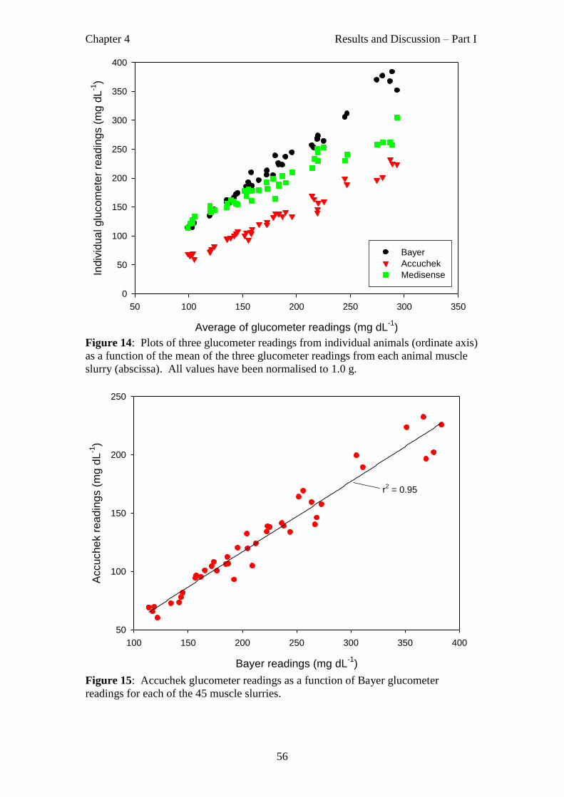
Chapter 4 Results and Discussion – Part I
56
Figure 14: Plots of three glucometer readings from individual animals (ordinate axis)
as a function of the mean of the three glucometer readings from each animal muscle
slurry (abscissa). All values have been normalised to 1.0 g.
Figure 15: Accuchek glucometer readings as a function of Bayer glucometer
readings for each of the 45 muscle slurries.
Average of glucometer readings (mg dL-1
)
50 100 150 200 250 300 350
Ind
ivid
ua
l g
luco
me
ter
rea
din
gs (
mg
dL
-1)
0
50
100
150
200
250
300
350
400
Bayer
Accuchek
Medisense
Bayer readings (mg dL-1
)
100 150 200 250 300 350 400
Accuche
k r
ead
ing
s (
mg
dL
-1)
50
100
150
200
250
r2 = 0.95

Chapter 4 Results and Discussion – Part I
57
Figure 16: Medisense glucometer readings as a function of Bayer glucometer readings for each of 45 muscle slurries. A quadratic curve
described the relationship well (A). This curve could be linearised by taking the square root of the Bayer glucometer data (B).
Bayer readings (mg dL-1
)
100 150 200 250 300 350 400
Me
dis
en
se
rea
din
gs (
mg d
L-1
)
100
150
200
250
300
350
)-1dL (mg Bayer( Bayer
10 12 14 16 18 20
100
150
200
250
300
350
A - unadjusted values B - adjusted values
r2 = 0.89

Chapter 4 Results and Discussion – Part I
58
Inspection of Figures 12, 13 and 14 shows that the three meters do not usually
return accurate values of glucose concentration. Moreover each glucometer behaves
differently in slope and in offset from the origin (e.g. the constant in a linear
equation). Thus they behave differently when the glucose is in a matrix other than
blood. Other researchers have obtained parallel results to those reported here
(Gardner, Moreland, & Thomson, 2004; Young, West, Hart, & Otterdijk, 2004).
There are several possible reasons for why the responses in blood and RpH buffer
could be different. The glucometer sensors are sensitive to liquid viscosity, and it is
likely that the viscosity of the liquid phase of slurry that enters the minute sensor
cavity would be lower than that of blood. The RpH buffer contains high
concentrations of acetate, while the tonicity of blood is that of normal saline.
Moreover, the pH values of blood and RpH buffer are very different, about 7.0 and
5.0 respectively. The temperature within the full sensor chamber is likely to be
slightly different for the two liquids having originated at 37°C (blood) and 55°C (meat
slurries).
Although the responses of glucometers to glucose in RpH buffer and blood are
different, the dynamic responses in RpH buffer and their precisions show that either
the Accuchek or the Medisense glucometer could contend to replace the Bayer
glucometer. Arguably, the linearity or otherwise of glucometer responses is
unimportant because in the practical application of the RpH technology it is only
necessary to determine if the Bayer glucose reading (normalised to 1 g of muscle) is
greater or less than 130 mg dL-1
. Provided the slope of the response curve is
approximately linear around that value, nothing else is important from a commercial
perspective. However, the interests of meat science will be better served with a
glucometer that is linear over a wide dynamic range. There was strong linear
relationship between the Bayer and Accuchek readings (Figure 15). The Medisense
values were closer to those of the Bayer glucometer, especially at lower glucose
concentrations (Figures 12 and 14), but were non-linear. Either glucometer could be
commercially useful, but the linearity of Accuchek glucometer would make it the
meter of choice. But there are other factors to consider. These are ease of use in an
abattoir environment and price.
Bayer glucometers were easy to use in the abattoir because the test strips are
arranged in a sealed carousel disc. One disc was enough for 10 readings (10 animals)
before the disc had to be replaced. Readings take approximately 30 seconds.

Chapter 4 Results and Discussion – Part I
59
The Accuchek glucometer take 20 seconds to return a reading. Test strips are
held in batches of 50 in a cylindrical plastic container, and each test strip has to be
individually inserted into the glucometer for each reading. This consumes time but is
unavoidable. The Medisense glucometer takes only 10 seconds to return a reading,
but test strips are individually wrapped and valuable time would be lost unwrapping
each test strip prior to individual insertion. The 10 second response time of the
Medisense glucometer might seem to be an advantage but in an abattoir environment
that is not the case. The incubation time of the sensor is not dead time because other
activities can be and are done in that window of opportunity.
Comparison of glucometer prices found that Accuchek glucometers are more
expensive than Medisense glucometers. When purchased directly from the suppliers,
the glucometer starter kits retail for $34.95 and $22.17, respectively. However, given
that a meter will last for many months, the difference in price is not important. In
contrast, the price of the test strips is important because each test is a consumable
cost. As quoted by the suppliers in early 2008, Accuchek strips cost $22.50 for a pack
of 50 strips, and Medisense strips cost $22.00. But these quoted values may be
misleading because a better price could probably be negotiated when buying in the
bulk that a beef processing company would consume in a year. (In this respect the
suppliers, Roche and Abbott, are unaware of the comparative data in this thesis and as
such are in a weak bargaining position.) The price of the test strips is very important
because consumables savings mount up in the long run.
Subject to test strip price, Accuchek appears to be the best replacement for the
Bayer glucometer. Gardner et al. (2004) found that Accuchek was able to
qualitatively predict high ultimate pH carcasses with 80% accuracy. Although the
aims of that study were rather different aims of those the present research, that study
indicates that the Accuchek glucometer would be suitable. It also has a higher upper
dynamic range limit than the current Bayer glucometer, which as discussed earlier is
useful from a meat science perspective. At the low concentration end of the dynamic
range the Bayer and Medisense meters are slightly more sensitive than the Accuchek.
This is shown in Figure 13 where an error message was returned by Accuchek at zero
added glucose, but not by the other two meters. However this does not detract from
Accuchek‟s desirability. The normalised quality threshold value used commercially
is 130 mg dL-1
with the Bayer glucometer (Young, Thomson et al., 2004). Inspection
of Figure 15 shows that the equivalent Accuchek result would be approximately

Chapter 4 Results and Discussion – Part I
60
70 mg dL-1
. Accuchek‟s lower detection limit lies somewhere between 0 and 50 mg
spiked glucose dL-1
as displayed by that meter (Figure 13)
In respect of the lower limit of detection, only five samples were identified as
high pH carcasses with Bayer glucose readings below 130 mg dL-1
. It was hoped that
sampling different animal classes (steers, cows and bulls) would capture the whole
spectrum of glucose values observed in beef in New Zealand. This was unfortunate
but nothing can be done about this. With very little data below the quality threshold
value of 130 mg dL-1
(Bayer) in Figure 15, one cannot be certain that data below this
point would still follow the linear correlation between Bayer and Accuchek data
(Figure 15). However, the curves in Figure 12, 13 and 14 strongly support the notion
that linearity continues to low concentrations. With this assumption, the equivalent
Accuchek threshold value was calculated by extrapolating the regression line of
existing between Bayer and Accuchek (Figure 15). The new cut-off value for pre-
rigor muscle using Accuchek glucometers is now set at 74.8 mg dL-1
. This is the
equivalent Accuchek reading for the old Bayer threshold.
For the RpH method to be useful to meat processors, proper training of staff
members who carry out the RpH method is essential. Several visits to commercial
abattoirs that employ the RpH method revealed significant inconsistencies such as
sampling of the wrong muscle, overheating of the meat slurry and the use of a faulty
homogeniser that did not completely disperse the meat sample. These and other
errors give unreliable results rendering the RpH method less useful as a quality
control tool. However, as pointed out by Young et al. (2004), most of the possible
errors in technique yield lower than actual glucose values. In this respect, the method
tends to „fail safe‟ in that low pH animals are more likely to be classed as high pH
animals than the other way around. However, that can adversely affect profit. At all
times the abattoir should aim for an accurate classification.
Although the RpH method is a relatively simple method of rapidly measuring
glycogen in pre-rigor muscle, the inherent cost of applying the method is a perceived
disadvantage. The current trend of glucometer manufacturers replacing old
glucometer models with newer ones (as experienced in this thesis) is also an issue and
recalibrating the RpH method with new glucometer models is costly and inconvenient
to meat processors. Even with the costs taken into account, the RpH method it is still
a worthwhile investment for the meat processors that use it. However, it would be
good to find a method that reduces the cost of the method.

Chapter 4 Results and Discussion – Part I
61
It has been proposed that near infra-red (NIR) spectroscopy could be a cheaper
and more robust method for rapidly measuring glycogen in pre-rigor meat. Although
the initial cost of purchasing a NIR spectrophotometer would be high, NIR
instruments are more cost effective in the long run as they are longer lasting and can
be specifically designed for industrial use. For NIR to be successfully applied on-line
to measure glycogen, calibration and validation steps are required. This firstly
involves finding a reliable reference glycogen determination method. Secondly,
developing predictive models to quantify glycogen in pre-rigor muscle collected on-
line. These are the objectives of the following chapter.

Chapter 5 Results and Discussion – Part II
62
CHAPTER 5
RESULTS AND DISCUSSION – PART II
COMPARISON OF THREE GLYCOGEN DETERMINATION METHODS
With the high collective costs of running the Rapid pH (RpH) method and the
inconvenience experienced by meat processors in calibrating the RpH method with
new glucometer models, it has been proposed that that near infra-red (NIR)
spectroscopy is ultimately a better method of rapidly measuring glycogen in pre-rigor
meat. The overall aim of this chapter is to develop predictive models to quantify
glycogen in M. logissimus dorsi (LD) muscle from NIR spectra collected on-line.
Developing models to measure glycogen first requires a reference glycogen
determination method that is reliable and precise. The first part of this chapter
describes work to find an accurate and consistent reference method from three popular
glycogen determination methods. Once a reference glycogen method has been found,
the final objective is to develop calibration models to measure glycogen concentration
and pH at approximately 45 minutes post-mortem (pH45) and to predict ultimate pH
(pHu) of pre-rigor LD muscles from NIR spectra collected on-line.
Determination of glycogen in M. longissimus dorsi
M. longissimus dorsi (LD) from three cows were collected less than one hour
after slaughter and stored in a 5°C chiller. Portions from each muscle were sub-
sampled at 1, 4, 9 and 20 hours post-mortem. The glycogen content of the LD
samples at each timepoint was then assayed using the Iodine, Bergmeyer and RpH
methods, all described in Chapter 3. The glucose content (originally glycogen) of the
LD samples analysed using the RpH method was calculated in mole terms using the
equation of the standard curve obtained from spiked meat slurries. For reasons
discussed later, the meter used for this technique was the Medisense glucometer. The
Bergmeyer method is similarly an enzymatic method that also expresses glycogen
content as glucose units in mole terms. Glycogen values from the Bergmeyer method
were converted into glycogen content in mass terms using the multiplication factor of

Chapter 5 Results and Discussion – Part II
63
Timepoint (hours postmortem)
0 5 10 15 20 25
Gly
co
ge
n (
mg
g-1
)
0
1
2
3
4
5
6
7
8
Iodine
Bergmeyer
Rapid pH
0.0162 (Keppler & Decker, 1974). The Iodine method expresses glycogen content
directly as glycogen determined by colorimetry based on iodine‟s reaction with
glycogen. Six replicates were conducted for each LD sample at each time point for
each method. Finally glycogen values were expressed as mg g-1
fresh weight of
muscle.
Figure 17 shows that the loss of glycogen by glycolysis during the onset of rigor
was detected by all methods. A major decrease in glycogen concentration was
observed within the first nine hours post-mortem, but less so when measured by the
RpH method. Between nine and 20 hours post-mortem, the changes in glycogen
concentration as measured by each method were essentially unchanging, such that at
20 hours the measured concentration by RpH was about three times higher than for
the other two methods.
Figure 17: Mean glycogen values of longissimus dorsi muscle samples and their
corresponding standard deviations at different time points post-mortem. Three
glycogen determination methods were compared.

Chapter 5 Results and Discussion – Part II
64
The fact that the Iodine and Bergmeyer methods gave similar results, and were
consistent with the known pattern of glycogen depletion after slaughter (Dreiling et
al., 1987; Young, West et al., 2004) suggests that these two methods gave more
believable results. It also implies that one of these is most likely to be the reference
glycogen determination method. However, accuracy is arguably less important than
precision in a reference method, so percent variances were calculated at each time
point (Table 1).
Table 1: Percent variances of glycogen concentration in longissimus dorsi muscle
samples at different timepoints post-mortem as measured by three methods
Timepoint
(hours postmortem) Iodine Bergmeyer Rapid pH
1 9.2 19.3 10.5
4 12.7 27.3 10.5
9 7.2 9 6.3
20 11.4 17.4 6.5
Mean percent variance
± SD
10.1 ± 18.3 ± 8.5 ±
There was no obvious trend in percent variance with time. The Bergmeyer
method yielded the most variable results, with little difference between the Iodine and
RpH methods. At this point the Iodine method appeared to be the method of choice.
Final choice of glycogen reference method for NIR calibration
It is important to reiterate that a new Medisense glucometer (Medisense Optium
Xceed™) was used in this section to determine glucose values through the RpH
method. Although Accuchek was originally suggested to replace Bayer (see previous
section), the manufacturers of Accuchek glucometers announced the replacement of
the recommended model with a newer model just weeks after the glucometer work in
the previous section was completed. Preliminary assessments of the new Accuchek
model found that it was not able to measure glucose in meat slurries at the pH of the
RpH buffer. Coincidentally during this period, a new Medisense model became
commercially available. Although it exhibited the non-linear response in meat
slurries as observed in the older model, it was the only commercial glucometer

Chapter 5 Results and Discussion – Part II
65
available at the time that was able to measure glucose in RpH buffer. It was therefore
the only viable replacement for the Accuchek glucometer recommended in the
previous section.
The purpose of comparing the three glycogen measurement methods was to
determine which method would be able to measure a range of glycogen values most
consistently, and so become the reference glycogen method for the NIR calibration
work (next section). Because glycogen in the muscles of freshly slaughtered
carcasses can be variable depending on the psychological and physiological state of
the animal before and at the time of slaughter, a method that could consistently
quantify glycogen at over a wide range of values was required.
Previous research on glycogen methods support the findings reported in this
section. The depletion of glycogen as monitored by the Iodine and Bergmeyer
methods at increasing timepoints follows the trend reported by Dreiling et al. (1987)
and Young et al. (2004). The glycogen content measured at both 1 hour and 24 hours
post-mortem for the Iodine and Bergmeyer methods also agree with results published
by Fabiansson and Reuterswärd (1984) and Dreiling et al (1987). However, some
studies (Immonen, Kauffman, Schaefer, & Puolanne, 2000; Lahucky et al., 1998;
Young, Thomson et al., 2004) have reported significantly higher levels of glycogen
one hour post-slaughter. This difference may be due to the analysis of a different
muscle, animal variation, variability in sample collection and preparation, or the
particular glycogen method used.
Results from the RpH method show that the glycogen results stabilised at
approximately 3.5 mg g-1
at 10 hours post-mortem. These results do not agree with
previous research that have found glycogen content in muscle from unstressed
animals approximately 24 hours post-mortem to be in the within 1 and 3 mg g-1
(Dreiling et al., 1987; Fabiansson & Reuterswärd, 1984; Lahucky et al., 1998). This
suggests that the RpH method may not give accurate results at low levels of glycogen.
These high readings may be due to errors introduced by the new Medisense
glucometer. The behaviour of this glucometer at low glycogen concentrations in meat
slurry needs to be further evaluated. Because of this uncertainty due to the high
readings at low levels of glycogen obtained, the RpH method was not chosen for the
calibration of the NIR instrument in the next section.
After assessing glycogen determination methods in post-mortem beef muscles,
Fabiansson and Reuterswärd (1984) suggested that enzymatic hydrolysis of glycogen

Chapter 5 Results and Discussion – Part II
66
followed by measurement of glucose by the Bergmeyer method as the best way of
measuring glycogen. However, a later study comparing the reliability of the Iodine
and Bergmeyer methods to measure glycogen in meat samples (Dreiling et al., 1987)
found that the Iodine method gave more consistent results than the Bergmeyer
method. The results reported in this section agree with this study. Although the mean
glycogen measurements for both methods in each timepoint were statistically similar
(p > 0.05), the mean percent variance for the Iodine method was numerically lower
than for the Bergmeyer method (Table 1), but this difference was not statistically
significant ( p = 0.085).
Although there was no statistical significance in the consistency of the Iodine
and Bergmeyer methods, the Iodine method protocol is simpler and less time
consuming than the enzymatic Bergmeyer method. Because of its simplicity and
higher precision, the Iodine method was chosen over the Bergmeyer and RpH
methods as the reference glycogen method to calibrate the NIR instrument for
glycogen determination in pre-rigor muscle.
The following section of this chapter details work to determine the efficacy of
NIR spectroscopy as an on-line method of rapidly measuring glycogen in a
commercial abattoir. The results of this objective are presented in the following
section where the NIR spectra were collected on-line and their glycogen content
subsequently determined using the Iodine method.
NEAR-INFRARED SPECTROSCOPY
Near-infrared scanning of muscles and selection of scans for data analysis
M. longissimus dorsi from 95 animals were scanned. In an effort to ensure that
a wide range of range of glycogen, pH at approximately 45 minutes post-mortem
(pH45) and ultimate pH (pHu) values were represented in the data set, spectra from
three animal classes (steers, bulls and cows) were collected. Twenty near-infrared
(NIR) scans between 538 and 1677 nm were recorded for each animal from a freshly
cut surface of the logissimus dorsi (LD) muscle between the 11th
and 12th
rib using the
reflectance probe described in Chapter 2.

Chapter 5 Results and Discussion – Part II
67
20 40 60 80 100 120 140
0.8
1.0
1.2
1.4
1.6
1.8
Ab
sorb
an
ce (
ab
sorb
an
ce u
nit
s)
Diode
20 40 60 80 100 120 140
0.8
1.0
1.2
1.4
1.6
1.8
Ab
sorb
an
ce (
ab
sorb
an
ce u
nit
s)
Diode
Figure 18: A typical plot showing the 20 near-infrared spectra collected from
prerigor M. longissimus dorsi muscle of one animal. The KES detector contained 152
diodes which covered the spectral range of 538 nm to 1677 nm.
Figure 18 shows there is variation in the spectra at different locations of the
same LD muscle, in this case, from a single animal. This is almost certainly due to
the heterogeneous nature of muscle where components such as collagen, fat and
connective tissue are more or less represented in given sections of the muscle.
Due to the variability of the NIR spectra collected from each animal, it is
important to identify spectra that are most representative of the muscle. As discussed
in Chapter 3, this was achieved by applying Principal Component Analysis (PCA) to
identify the 10 most similar spectra from the 20 collected from each animal. Figure
19A shows the 10 spectra that were selected using PCA. The mean of these spectra
were averaged to give a representative spectrum for the animal (Figure 19B). The 95
mean spectra from each animal were used for the subsequent development of models
to quantify glycogen in pre-rigor muscle, measure pH45 and predict the pHu and of
prerigor LD muscle.

Chapter 5 Results and Discussion – Part II
68
Figure 19: Principal Component Analysis of near-infrared (NIR) spectra showing the
10 selected spectra (A). The selected spectra were then averaged to give a
representative NIR spectrum for the animal.
20 40 60 80 100 120 140
0.8
1.0
1.2
1.4
1.6
1.8
Ab
sorb
ance
(ab
sorb
ance
un
its)
Diode
Selected spectra
Rejected spectra
A – Selected spectra
20 40 60 80 100 120 140
0.8
1.0
1.2
1.4
1.6
1.8
Ab
sorb
ance
(ab
sorb
ance
un
its)
Diode
Selected spectra
Rejected spectra
20 40 60 80 100 120 140
0.8
1.0
1.2
1.4
1.6
1.8
Ab
sorb
ance
(ab
sorb
ance
un
its)
Diode
Selected spectra
Rejected spectra
Selected spectra
Rejected spectra
A – Selected spectra
20 40 60 80 100 120 140
0.8
1.0
1.2
1.4
1.6
1.8
Ab
sorb
ance
(ab
sorb
ance
un
its)
Diode
Selected spectra
Rejected spectra
A – Selected spectra
20 40 60 80 100 120 140
0.8
1.0
1.2
1.4
1.6
1.8
Ab
sorb
ance
(ab
sorb
ance
un
its)
Diode
Selected spectra
Rejected spectra
20 40 60 80 100 120 140
0.8
1.0
1.2
1.4
1.6
1.8
Ab
sorb
ance
(ab
sorb
ance
un
its)
Diode
Selected spectra
Rejected spectra
Selected spectra
Rejected spectra
A – Selected spectra
20 40 60 80 100 120 140
0.8
1.0
1.2
1.4
1.6
1.8
Ab
sorb
ance
(ab
sorb
ance
un
its)
Diode
B – Average of selected spectra
20 40 60 80 100 120 140
0.8
1.0
1.2
1.4
1.6
1.8
Ab
sorb
ance
(ab
sorb
ance
un
its)
Diode
20 40 60 80 100 120 140
0.8
1.0
1.2
1.4
1.6
1.8
Ab
sorb
ance
(ab
sorb
ance
un
its)
Diode
B – Average of selected spectra
20 40 60 80 100 120 140
0.8
1.0
1.2
1.4
1.6
1.8
Ab
sorb
ance
(ab
sorb
ance
un
its)
Diode
B – Average of selected spectra
20 40 60 80 100 120 140
0.8
1.0
1.2
1.4
1.6
1.8
Ab
sorb
ance
(ab
sorb
ance
un
its)
Diode
20 40 60 80 100 120 140
0.8
1.0
1.2
1.4
1.6
1.8
Ab
sorb
ance
(ab
sorb
ance
un
its)
Diode
B – Average of selected spectra
20 40 60 80 100 120 140
0.8
1.0
1.2
1.4
1.6
1.8
Ab
sorb
ance
(ab
sorb
ance
un
its)
Diode
Selected spectra
Rejected spectra
A – Selected spectra
20 40 60 80 100 120 140
0.8
1.0
1.2
1.4
1.6
1.8
Ab
sorb
ance
(ab
sorb
ance
un
its)
Diode
Selected spectra
Rejected spectra
20 40 60 80 100 120 140
0.8
1.0
1.2
1.4
1.6
1.8
Ab
sorb
ance
(ab
sorb
ance
un
its)
Diode
Selected spectra
Rejected spectra
Selected spectra
Rejected spectra
A – Selected spectra
20 40 60 80 100 120 140
0.8
1.0
1.2
1.4
1.6
1.8
Ab
sorb
ance
(ab
sorb
ance
un
its)
Diode
Selected spectra
Rejected spectra
A – Selected spectra
20 40 60 80 100 120 140
0.8
1.0
1.2
1.4
1.6
1.8
Ab
sorb
ance
(ab
sorb
ance
un
its)
Diode
Selected spectra
Rejected spectra
20 40 60 80 100 120 140
0.8
1.0
1.2
1.4
1.6
1.8
Ab
sorb
ance
(ab
sorb
ance
un
its)
Diode
Selected spectra
Rejected spectra
Selected spectra
Rejected spectra
A – Selected spectra
20 40 60 80 100 120 140
0.8
1.0
1.2
1.4
1.6
1.8
Ab
sorb
ance
(ab
sorb
ance
un
its)
Diode
Selected spectra
Rejected spectra
Selected spectra
Rejected spectra
20 40 60 80 100 120 140
0.8
1.0
1.2
1.4
1.6
1.8
Ab
sorb
ance
(ab
sorb
ance
un
its)
Diode
Selected spectra
Rejected spectra
Selected spectra
Rejected spectra
A – Selected spectra
Selected spectra
Rejected spectra
Selected spectra
Rejected spectra
A – Selected spectra
20 40 60 80 100 120 140
0.8
1.0
1.2
1.4
1.6
1.8
Ab
sorb
ance
(ab
sorb
ance
un
its)
Diode
Selected spectra
Rejected spectra
20 40 60 80 100 120 140
0.8
1.0
1.2
1.4
1.6
1.8
Ab
sorb
ance
(ab
sorb
ance
un
its)
Diode
Selected spectra
Rejected spectra
Selected spectra
Rejected spectra
A – Selected spectra
20 40 60 80 100 120 140
0.8
1.0
1.2
1.4
1.6
1.8
Ab
sorb
ance
(ab
sorb
ance
un
its)
Diode
Selected spectra
Rejected spectra
Selected spectra
Rejected spectra
20 40 60 80 100 120 140
0.8
1.0
1.2
1.4
1.6
1.8
Ab
sorb
ance
(ab
sorb
ance
un
its)
Diode
Selected spectra
Rejected spectra
Selected spectra
Rejected spectra
A – Selected spectra
Selected spectra
Rejected spectra
Selected spectra
Rejected spectra
A – Selected spectra
20 40 60 80 100 120 140
0.8
1.0
1.2
1.4
1.6
1.8
Ab
sorb
ance
(ab
sorb
ance
un
its)
Diode
B – Average of selected spectra
20 40 60 80 100 120 140
0.8
1.0
1.2
1.4
1.6
1.8
Ab
sorb
ance
(ab
sorb
ance
un
its)
Diode
20 40 60 80 100 120 140
0.8
1.0
1.2
1.4
1.6
1.8
Ab
sorb
ance
(ab
sorb
ance
un
its)
Diode
B – Average of selected spectra
20 40 60 80 100 120 140
0.8
1.0
1.2
1.4
1.6
1.8
Ab
sorb
ance
(ab
sorb
ance
un
its)
Diode
B – Average of selected spectra
20 40 60 80 100 120 140
0.8
1.0
1.2
1.4
1.6
1.8
Ab
sorb
ance
(ab
sorb
ance
un
its)
Diode
20 40 60 80 100 120 140
0.8
1.0
1.2
1.4
1.6
1.8
Ab
sorb
ance
(ab
sorb
ance
un
its)
Diode
B – Average of selected spectra
20 40 60 80 100 120 140
0.8
1.0
1.2
1.4
1.6
1.8
Ab
sorb
ance
(ab
sorb
ance
un
its)
Diode
B – Average of selected spectra
20 40 60 80 100 120 140
0.8
1.0
1.2
1.4
1.6
1.8
Ab
sorb
ance
(ab
sorb
ance
un
its)
Diode
20 40 60 80 100 120 140
0.8
1.0
1.2
1.4
1.6
1.8
Ab
sorb
ance
(ab
sorb
ance
un
its)
Diode
B – Average of selected spectra
20 40 60 80 100 120 140
0.8
1.0
1.2
1.4
1.6
1.8
Ab
sorb
ance
(ab
sorb
ance
un
its)
Diode
20 40 60 80 100 120 140
0.8
1.0
1.2
1.4
1.6
1.8
Ab
sorb
ance
(ab
sorb
ance
un
its)
Diode
B – Average of selected spectra
20 40 60 80 100 120 140
0.8
1.0
1.2
1.4
1.6
1.8
Ab
sorb
ance
(ab
sorb
ance
un
its)
Diode
20 40 60 80 100 120 140
0.8
1.0
1.2
1.4
1.6
1.8
Ab
sorb
ance
(ab
sorb
ance
un
its)
Diode
B – Average of selected spectra
20 40 60 80 100 120 140
0.8
1.0
1.2
1.4
1.6
1.8
Ab
sorb
ance
(ab
sorb
ance
un
its)
Diode
20 40 60 80 100 120 140
0.8
1.0
1.2
1.4
1.6
1.8
Ab
sorb
ance
(ab
sorb
ance
un
its)
Diode
B – Average of selected spectra
20 40 60 80 100 120 140
0.8
1.0
1.2
1.4
1.6
1.8
Ab
sorb
ance
(ab
sorb
ance
un
its)
Diode
20 40 60 80 100 120 140
0.8
1.0
1.2
1.4
1.6
1.8
Ab
sorb
ance
(ab
sorb
ance
un
its)
Diode
B – Average of selected spectra
20 40 60 80 100 120 140
0.8
1.0
1.2
1.4
1.6
1.8
Ab
sorb
ance
(ab
sorb
ance
un
its)
Diode
20 40 60 80 100 120 140
0.8
1.0
1.2
1.4
1.6
1.8
Ab
sorb
ance
(ab
sorb
ance
un
its)
Diode
B – Average of selected spectra
20 40 60 80 100 120 140
0.8
1.0
1.2
1.4
1.6
1.8
Ab
sorb
ance
(ab
sorb
ance
un
its)
Diode
20 40 60 80 100 120 140
0.8
1.0
1.2
1.4
1.6
1.8
Ab
sorb
ance
(ab
sorb
ance
un
its)
Diode
B – Average of selected spectra

Chapter 5 Results and Discussion – Part II
69
Development of calibration models to measure the glycogen concentration and
pH45 and predict pHu in pre-rigor muscle
Any capability of NIR to quantify glycogen in pre-rigor muscle is based on the
assumption that glycogen affects the scattering and absorption of light in the NIR
region. This would be due to the ability of glycogen, a polymer of glucose, to absorb
or reflect light at particular NIR wavelengths characteristic to the molecule. As light
is beamed into a muscle, it is scattered, and either absorbed or reflected back into the
probe where it reaches the detector to produce a signal. The reflectance spectrum is
proportional in some way to the concentration of glycogen in the muscle. At the same
time, the reflectance spectrum can be used to calculate the NIR light absorbed by the
muscle because the spectral characteristics of the light generated by the probe are
completely known.
Partial least squares (PLS) regression is a statistical technique that assumes a
linear relationship exists between the spectral data and the parameter of interest. In
this thesis, PLS was used to develop linear models that predict glycogen
concentrations, pH45 and pHu in prerigor LD muscle. Successful predictive models
for these parameters rely upon the NIR instrument being able to detect spectral
variation as reference measurements changes from sample to sample.
For models generated using PLS regression, a linear model is applied to identify
if any significant covariation between predicted and measured values exist. This is
achieved by dividing the data into two sets – one set for calibration the other set for
validation. The calibration set is used to generate the model while the validation set
evaluates whether the model can be applied to new samples independent from those
used to construct the model. As outlined in Chapter 3, the capability of the PLS
models that were developed was tested with leave-one-out cross validation.
PLS models are assumed to be directly influenced by a number of latent
variables (LVs). In contrast to measured variables (glycogen, pHu and pH45), latent
variables are not directly observed. Rather, they are underlying variables which are
assumed to be directly related observed variables and NIR spectra. The number of
LVs influencing a model us usually not known, and the aim of PLS is to estimate the
number of LVs that give the optimum predictive model.
The significance of a model is verified mainly by their Mean Square Error of
Prediction (MSEP) and coefficient of determination (r2) values. MSEP is an indicator
of how accurate the model is at predicting the values of independent samples

Chapter 5 Results and Discussion – Part II
70
compared to their reference measurements. The significance of a model is also
indicated by the covariation between the predicted values and measured values. If
significant covariation in a model exists, a high r2 value is attained.
The generated models were verified by plotting „predicted‟ against „measured‟
values. In an accurate model where significant covariation exists, the points in the
plot will form a linear trend and plot over a 45° line. Hence optimum predictive
models are identified by the number of latent variables that have the maximum r2 and
the least MSEP from leave-one-out cross validation predictions.
Predictive models for glycogen measurement were determined from both the
absorbance and reflectance spectra to determine which spectral data generated better
models. Table 2 shows that models generated from reflectance spectra gave better
results for glycogen, pHu, and pH45 and so the reflectance spectra was used to
generate PLS models for their prediction in pre-rigor muscle.
Table 2: Summary of results for PLS models fitted to predict glycogen, pHu and pH45
in pre-rigor LD muscle by leave-out-one cross validation. Models generated
from reflectance spectra gave slightly better models
Spectra (538 to 1677 nm)
Prediction from absorbance Prediction from reflectance
LVa 11 6 10 13 6 0.13
r2b
0.22 0.18 0.31 0.23 0.20 0.37
MSEPc
7.75 0.13 0.04 7.75 0.13 0.04
a LV: Number of latent variables in fitted model
b r
2: coefficient of determination
c MSEP: Mean square error of prediction for cross validation predictions

Chapter 5 Results and Discussion – Part II
71
Figure 20: Mean Square Error of Prediction (MSEP) (A) and coefficient of determination (r2) (B) values of Partial Least Squares (PLS) models
of the reflectance spectra (538 to 1677 nm) for the prediction of glycogen in pre-rigor muscle. Predictions of leave-one-out cross validation are
presented in terms of measured and predicted glycogen values. Thirteen latent variables were used to generate the optimum PLS model.
Latent Variables0 5 10 15 20
r2
0.00
0.05
0.10
0.15
0.20
0.25
B
Latent Variables0 5 10 15 20
MS
EP
7.5
8.0
8.5
9.0
9.5
10.0
10.5
11.0
A
Measured Glycogen (mg g-1
)
0 2 4 6 8 10 12 14
Pre
dic
ted
Gly
co
ge
n (
mg
g-1
)
0
2
4
6
8
10
12
14
Bull
Cow
Steer
C

Chapter 5 Results and Discussion – Part II
72
The PLS calibration models for glycogen determination were poor. The optimal
calibration model from the reflectance spectra had 13 latent variables which gave an
r2 of 0.23 and a large MSEP of 7.75 mg g
-1 (Figure 20). The r
2 value of 0.23 indicates
that the best attainable calibration model for glycogen can explain only 23 percent of
the variation in the predicted glycogen values. The optimal calibration model from
the absorbance spectra was statistically very similar to the reflectance spectra with a
lower r2 of 0.22.
The best calibration model fitted to predict pHu from reflectance spectra was
also very poor. Cross validation predictions yielded a very low r2 of 0.20 with an
MSEP of 0.13. The regression plot (Figure 21C) shows that the pHu of most steers
and cows fall below pH 5.7 with a predicted pHu ranging from approximately pH 5.2
to 6.0. It also shows that the distribution of the pHu of bulls was different from that of
steers and cows. Although the measured pHu of the bulls ranged between pH 5.5 and
6.8, the predicted pHu of most bulls was within the narrow pH range of 5.7 to 6.2.
This suggests that a separate calibration model may need to be fitted for bulls to
predict pHu. Inspection of Figure 20C shows no obvious differences between the
three gender classes that could be exploited in developing gender-specific calibration
models for glycogen prediction. However, the regression plot of predicted pHu from
the reflectance spectra (Figure 21C) show that the bulls, cows and steers each follow a
different trend which suggests that a different model may be required for each animal
class.
PLS models were also developed to predict pH45. Validation was performed to
find the model with the optimum number of latent variables that produced the
maximum r2 and the lowest MSEP (Figure 22). Results from the reflectance spectra
show that the best attainable calibration model was still poor (r2 = 0.37). Although
the MSEP of the model after cross validation was very low (0.039), only 37 percent of
the variation in the pH45 of muscle could be explained by the calibration model.
The regression plot of muscle at pH45 (Figure 22C) show that data tend to be
clustered according to animal class. Most bulls had a measured and predicted pH45
value above 6.5, while almost all steers had measured and predicted pH45 values
ranging from 5.9 to 6.6. Again this suggests that separate models might need to be
fitted to the different animal classes.

Chapter 5 Results and Discussion – Part II
73
Figure 21: Mean Square Error of Prediction (MSEP) (A) and coefficient of determination (r2) (B) values of Partial Least Squares (PLS) models
of the reflectance spectra (538 to 1677 nm) for the prediction of ultimate pH (pHu) in pre-rigor muscle. Predictions of leave-one-out cross
validation are presented in terms of measured and predicted pHu values. Six latent variables were used to generate the optimum PLS model.
Samples for pHu measurements were frozen in liquid nitrogen and the pHu measured a month later.
Latent Variables
0 5 10 15 20
r2
0.00
0.05
0.10
0.15
0.20
0.25
B
Measured pHu
5.0 5.2 5.4 5.6 5.8 6.0 6.2 6.4 6.6 6.8 7.0
Pre
dic
ted p
Hu
5.0
5.2
5.4
5.6
5.8
6.0
6.2
6.4
6.6
6.8
7.0
Bull
Cow
Steer
C
Latent Variables
0 5 10 15 20
MS
EP
0.12
0.13
0.14
0.15
0.16
0.17
0.18
0.19
0.20
A

Chapter 5 Results and Discussion – Part II
74
Figure 22: Mean Square Error of Prediction (MSEP) (A) and coefficient of determination (r2) (B) values of Partial Least Squares (PLS) models
of the reflectance spectra (538 to 1677 nm) for the prediction of pH45 in pre-rigor muscle. Predictions of leave-one-out cross validation are
presented in terms of measured and predicted pH at approximately 45 minutes post-mortem (pH45) values. Thirteen latent variables were used to
generate the optimum PLS model (C). pH45 was measured in the abattoir immediately after near-infrared scanning.
Latent Variables
0 5 10 15 20
r2
0.00
0.05
0.10
0.15
0.20
0.25
0.30
0.35
0.40
B
Latent Variables
0 5 10 15 20
MS
EP
0.036
0.038
0.040
0.042
0.044
0.046
0.048
0.050
0.052
0.054
A
Measured pH45
5.8 6.0 6.2 6.4 6.6 6.8 7.0
Pre
dic
ted p
H4
5
5.8
6.0
6.2
6.4
6.6
6.8
7.0
Bull
Cow
Steer
C

Chapter 5 Results and Discussion – Part II
75
Development of classification models to categorise meat into two classes of pHu
As presented in the previous section, PLS models generated to predict muscle
glycogen were very poor. Determining the glycogen concentration of muscle is
ultimately not useful for meat processors. They only want to know whether a carcass
will be above the acceptable threshold of pHu. Thus the development of models to
classify meat into two pHu categories was attempted in this section.
As discussed in the earlier, Generalised partial least squares (GPLS) was used to
develop classification models to categorise beef carcasses into their predicted pHu.
GPLS is similar to PLS modelling. However, GPLS algorithms are specifically for
constructing classification models and are different from that of PLS.
GPLS classification models were achieved by dividing the reflectance data set
into two sets one for calibration and the other for validation. Seventy-five percent of
the data set (72 animals) was randomly chosen to produce calibration models. The
remaining 24 animals were used as an independent data set for validation.
Two models were developed, the first where gender was taken into account, and
the second where the gender effect was removed.
As described in Chapter 2, the gender-into-account model first involved dividing
the range of pHu data into four groups (quartiles), with 75 percent of the data from
each quartile allocated randomly to form the calibration data set. The calibration data
set was used to fit a linear model to estimate the probability of a sample to have a pHu
greater than 5.7. The independent validation set was then fitted to the model to test
the model‟s accuracy at classifying the pHu of prerigor muscle. Three hundred (15
LVs 20 models) models were fitted. Twenty models were attempted at each LV as
models generated beyond this were not significantly different from the twentieth
model.
For the second model, the gender effect was reduced by splitting spectra in three
subsets (bulls, cows and steers). The average spectra of each subset was calculated
and then subtracted from spectra in the corresponding subset. Calibration and
validation of was carried out as for the gender-into-account model.

Chapter 5 Results and Discussion – Part II
76
Figure 23: Calibration model (A) and validation (B) of classification models with gender effect taken into account. Classification was based on
the probability of samples reaching an ultimate pH (pHu) lower than 5.7. The reflectance spectra were used with nine latent variables giving the
optimum model.
Measured pHu
4.5 5.0 5.5 6.0 6.5 7.0
Pro
ba
bility to b
e <
pH
u 5
.7
0.0
0.2
0.4
0.6
0.8
1.0
Bull
Cow
Steer
A
Measured pHu
4.5 5.0 5.5 6.0 6.5 7.0
0.0
0.2
0.4
0.6
0.8
1.0
Bull
Cow
Steer
B

Chapter 5 Results and Discussion – Part II
77
Figure 24: Calibration model (A) and validation (B) of classification models after ignoring the gender effect. Classification was based on the
probability of samples reaching an ultimate pH (pHu) lower than 5.7. The reflectance spectra were used with nine latent variables giving the
optimum model.
Measured pHu
4.5 5.0 5.5 6.0 6.5 7.0
0.0
0.2
0.4
0.6
0.8
1.0
Bull
Cow
Steer
B
Measured pHu
4.5 5.0 5.5 6.0 6.5 7.0
Pro
bab
ility to b
e <
pH
u 5
.7
0.0
0.2
0.4
0.6
0.8
1.0
Bull
Cow
Steer
A

Chapter 5 Results and Discussion – Part II
78
Table 3: Percentage of correct and incorrect classification of calibration and validation data for GPLS classification models
with the inclusion and exclusion of gender effects. The reflectance data was used with nine LVs giving the optimum
model
Gender effect included Gender effect excluded
Calibration Validation Calibration Validation
Low pH High pH Low pH High pH Low pH High pH Low pH High pH
Correct classification (%) 98 61 83 42 94 39 85 21
Incorrect classification (%) 2 39 17 58 6 61 15 79

Chapter 5 Results and Discussion – Part II
79
Bull data from the calibration and validation GPLS models exhibited a different
trend from steers and cows (Figure 23). Most of the data with measured and predicted
pHu values above 5.7 were predominantly from bulls. This confirms findings from
the previous predictive PLS models for glycogen, pH45 and pHu and suggests that
since the trend and pHu profile of bulls are different, they may require a separate
GPLS model to predict their pHu.
Table 3 shows that the classification models yielded poor results. For the first
model, where gender was taken into account, most of the calibration data with normal
pHu were fitted well by the model: 98% of the calibration data was correctly classified
for all models fitted which suggests that the GPLS calibration model is good at
predicting muscle that will reach a normal pHu correctly. However, a significant
proportion of the calibration data (39%) with a high pHu did not correctly fit the
model. When the independent data (validation) was fitted into the calibration models,
poorer results were obtained. For normal pH samples, 83 percent of the validation
samples were correctly classified as normal pHu. However, at high pH, only 42% of
the validation samples were correctly classified.
When the effect of gender was removed (Figure 24), an even a poorer
classification model was generated. Most of the calibration data fitted correctly into
the model at normal pHu, but only 39% of the calibration model fitted correctly at
high pHu. The poor calibration model resulted in most of the validation data being
classified wrongly at the high pHu range where only 21% of high pHu animals were
classified correctly.
Exploratory analysis of NIR spectra to evaluate factors that give differences
between genders
Attempts to develop models that quantify glycogen in prerigor muscle or predict
pHu of muscle from NIR spectra collected on-line have been unsuccessful thus far. In
order to explain why such poor models were attained, and in an attempt to extract
additional information from the spectra, exploratory analysis of the NIR spectra was
conducted.
The method for exploratory analysis of the NIR spectra using Hierarchical
Cluster Analysis (HCA) was described in Chapter 2. Briefly, HCA is a technique
which primarily aims to present data in a manner which emphasises natural

Chapter 5 Results and Discussion – Part II
80
groupings. The distances between the spectra on a two, three or multi-dimensional
plot were calculated where naturally similar spectra are separated by small distances.
Once the distances between all spectra have been calculated, HCA results are
presented in the form of a dendrogram to facilitate the recognition of groups within
the data (Figure 25).
Figure 25: Illustration of the exploratory analysis of a small data set (seven samples
described by two variables). Three groups are identified and are presented
accordingly in a dendrogram (b). Group 1 (Sample G) is characterised having the
lowest values for both variables. Group 2 (Samples A, C and B) is characterised by
having the highest values of variable 2 (VAR 2) and low values in variable 1 (VAR
1). Group 3 (Samples D, E and F) is characterised by samples with high values in
VAR 1 and low values in VAR 2.
In this thesis, HCA was conducted on the mean absorbance spectra to identify
groups of animals with naturally similar NIR spectra. The absorbance spectra were
chosen for HCA analysis because they were easier to manipulate and gave slightly
better results than the reflectance spectra. The first objective in HCA was to
determine a numerical value for the similarity between the mean absorbance spectra

Chapter 5 Results and Discussion – Part II
81
from each animal. As mentioned in Chapter 2, this was achieved by calculating the
Euclidean distances between pairs of samples. Euclidean distance is simply the
geometric distance between two data points in a space with any number of
dimensions. Once the distances between spectra were determined, spectra were then
divided into groups where the spectra in each group were naturally similar.
Exploratory analysis of the absorbance spectra from the beef samples show that
groups with naturally similar NIR spectra do exist. This is illustrated in the
dendrogram (Figure 26). Five distinct groups of animals were identified. Most of the
data can be distributed among Groups 1, 2 and 3. Although all animal classes are
present in all groups, it is evident that they are each more represented in certain
groups. The majority of Group 1 comprises bulls. Groups 2 and 3 are predominantly
comprised of steers; however, Group Three has a significant proportion of bulls and
cows. As only a few animals were classed into Groups 4 and 5, and both groups have
approximately the same proportion of animals found in Groups 2 and 3, these groups
may not bear the same statistical significance as Groups 1, 2 and 3.
After groups with naturally similar spectra were identified (Figure 26), the
comparison of glycogen, pHu, pH45, and live weight values of the animals within
those groups was conducted, as illustrated in the boxplots (Figure 27).
The results show that all groups have similar glycogen concentration with
approximate means between 6 and 8 mg g-1
. Although Group 1 has a greater range of
pHu values, the pHu average for all groups was approximately pH 5.5. Most groups
also showed similar pH at pH45. An interesting finding was the significantly lower
pH45 of animals in Group 2. The reason why this group, which is predominantly
comprised of steers, has a lower pH45 is unknown. However, the ability of NIR to
detect a difference in this group when the glycogen content and pHu of all groups
were very much the same is interesting.

Chapter 5 Results and Discussion – Part II
82
Figure 26: Hierarchical Cluster Analysis of the absorbance spectra (538 to 1677 nm) of pre-rigor LD muscle from 96 animals. The most
similar groups are arranged closer together. Thus Group 2 is the most similar group to Group 1, whereas Group 5 is the most dissimilar to
Group 1.
2-B
ull
2-C
ow
2-S
teer
2-B
ull 2
-Bull
2-B
ull
2-B
ull
2-S
teer
2-S
teer
2-S
teer
2-S
teer
2-B
ull
2-B
ull
2-B
ull
2-B
ull
2-C
ow
2-S
teer
2-S
teer
2-B
ull
2-B
ull
2-B
ull
2-S
teer
2-B
ull
2-C
ow
2-C
ow
2-B
ull
2-B
ull
2-C
ow
2-B
ull
2-B
ull
2-B
ull
2-B
ull
3-S
teer
3-S
teer
3-S
teer
3-S
teer
3-C
ow
3-C
ow 3
-Ste
er
3-S
teer
3-S
teer
3-S
teer
3-S
teer
3-S
teer
3-S
teer
3-S
teer
3-S
teer
3-S
teer
3-S
teer
3-S
teer
1-B
ull
1-C
ow 1
-Bull
1-C
ow 1-C
ow
1-S
teer
1-S
teer
1-S
teer
1-C
ow
1-S
teer
1-S
teer
1-S
teer
1-S
teer
1-B
ull
1-B
ull
1-S
teer
1-S
teer
1-B
ull
1-S
teer
1-S
teer
1-S
teer
1-S
teer
1-S
teer
1-S
teer
1-S
teer
1-B
ull
1-S
teer
1-B
ull
1-C
ow
1-C
ow 5
-Ste
er
5-C
ow
5-S
teer
5-S
teer
5-C
ow
5-S
teer
5-C
ow
4-C
ow
4-C
ow
4-S
teer
4-B
ull
4-C
ow
4-B
ull
4-S
teer
4-C
ow
Group 1 Group 2 Group 3 Group 4 Group 5
2-B
ull
2-C
ow
2-S
teer
2-B
ull 2
-Bull
2-B
ull
2-B
ull
2-S
teer
2-S
teer
2-S
teer
2-S
teer
2-B
ull
2-B
ull
2-B
ull
2-B
ull
2-C
ow
2-S
teer
2-S
teer
2-B
ull
2-B
ull
2-B
ull
2-S
teer
2-B
ull
2-C
ow
2-C
ow
2-B
ull
2-B
ull
2-C
ow
2-B
ull
2-B
ull
2-B
ull
2-B
ull
3-S
teer
3-S
teer
3-S
teer
3-S
teer
3-C
ow
3-C
ow 3
-Ste
er
3-S
teer
3-S
teer
3-S
teer
3-S
teer
3-S
teer
3-S
teer
3-S
teer
3-S
teer
3-S
teer
3-S
teer
3-S
teer
1-B
ull
1-C
ow 1
-Bull
1-C
ow 1-C
ow
1-S
teer
1-S
teer
1-S
teer
1-C
ow
1-S
teer
1-S
teer
1-S
teer
1-S
teer
1-B
ull
1-B
ull
1-S
teer
1-S
teer
1-B
ull
1-S
teer
1-S
teer
1-S
teer
1-S
teer
1-S
teer
1-S
teer
1-S
teer
1-B
ull
1-S
teer
1-B
ull
1-C
ow
1-C
ow 5
-Ste
er
5-C
ow
5-S
teer
5-S
teer
5-C
ow
5-S
teer
5-C
ow
4-C
ow
4-C
ow
4-S
teer
4-B
ull
4-C
ow
4-B
ull
4-S
teer
4-C
ow
Group 1 Group 2 Group 3 Group 4 Group 5

Chapter 5 Results and Discussion – Part II
83
Figure 27: Means of reference values for similar groups were been identified after Hierarchical Cluster Analysis of the absorbance spectra of 96
animals. Plot A represents glycogen concentration, Plot B ultimate pH, Plot C pH at approximately 45 minutes post-mortem (pH45), and Plot D
liveweight.
Liv
eW
t(K
g)
Liv
eW
t(K
g)
Liv
eW
t(K
g)
1 2 3 4 51 2 3 4 5
350
400
450
500
550
600
650
Groups
D
1 2 3 4 5
02
46
810
12
14
Groups
Gly
cogen(m
g/g
)
1 2 3 4 51 2 3 4 5
02
46
810
12
14
Groups
Gly
cogen(m
g/g
)
A
Ultim
ate
pH
Ultim
ate
pH
1 2 3 4 51 2 3 4 5
5.5
6.0
6.5
Groups
B
pH
45
pH
45
1 2 3 4 51 2 3 4 5
6.0
6.2
6.4
6.6
6.8
7.0
Groups
C

Chapter 5 Results and Discussion – Part II
84
Discussion
Some commercial abattoirs in New Zealand employ the current Rapid pH (RpH)
method as a discriminatory tool used to identify carcasses that will produce high pH
meat. Currently, the cut-off point for normal pH in some meat processing plants is
pH 5.7. Carcasses that are predicted to have an ultimate pH (pHu) greater than 5.7 are
separated and sold as manufacturing grade beef. For a number of technical and
economic reasons discussed in Chapter 1, it was decided to explore the potential for a
relatively non-invasive method of predicting pHu, based on NIR spectroscopy to
replace the RpH method.
A capability of NIR to predict glycogen and the pHu of pre-rigor muscle
assumes that variation in the glycogen concentration, or chemical composition
somehow related to pH in a muscle, can be reproducibly detected by NIR
spectroscopy. If this assumption were true, then the spectra collected from each
animal could be used to produce models that could ultimately predict glycogen and
pHu from a NIR scan taken immediately after slaughter. More formally, a successful
model using PLS and GPLS depends upon the covariation between laboratory
measurements of glycogen and pHu and their corresponding NIR spectra that were
collected on-line.
Two statistical models were developed in this thesis to predict pHu in pre-rigor
beef. These include Partial Least Squares (PLS) and generalised Partial Least Squares
(GPLS), the principles of which were described in Chapter 2 and summarised earlier
in this chapter.
Studies addressing the potential of NIR as a non-destructive method of
measuring pH have reported strong positive correlations between the measured pH
and predicted pH from statistical models generated from NIR specta (Andersen et al.,
1999; Andrés et al., 2007). However at present, there are no reports of the ability of
NIR to predict the pHu of a muscle from spectra collected on-line. Thus, this thesis
addressed the efficacy of a commercially available NIR instrument to quantify
glycogen and to predict the pHu of pre-rigor longissimus dorsi (LD) muscle. NIR
spectra of pre-rigor LD muscles were collected on-line in a commercial abattoir
approximately 45 minutes after slaughter.
Poor calibration models were generated using PLS to predict pre-rigor glycogen,
pH45, and pHu with a high prediction error observed for the glycogen model. A
different model may be needed for each animal class as their trends were distinctly

Chapter 5 Results and Discussion – Part II
85
different. The low r2 observed for steers, bulls and cows for the three attributes
measured after cross validation suggest PLS regression may not be the best approach
to generating a calibration model.
Andersen et al. (1999) and Andrés et al. (2007) have both explored NIR as a
non-invasive method of measuring pH one day after slaughter in pork and beef
respectively. Their calibration models that were generated using PLS had very good
prediction and little error with respective r2 of 0.80 and 0.97, and standard error of
predictions of 0.08 and 0.10 pH units.
Results from this thesis are not consistent with these findings. PLS models
generated from pH45 measurements showed a very weak r2 of 0.37. Even though the
measurements of pH and collection of NIR spectra was not carried out at the exact
timepoint (5 to 10 minutes difference), the capability of NIR to measure pH45 and
predict pHu was still very poor.
It is important to consider that the approaches to NIR pH measurement in this
project and the published studies are different. Published studies primarily focussed
on investigating the capability of NIR to measure meat pH in a controlled laboratory
environment after pHu has been attained. In contrast, the capability of NIR to
measure the pH45 of pre-rigor muscle in a realistic industrial situation was
investigated in this thesis. The superior PLS calibration models reported by Andersen
et al. (1999) and Andrés et al. (2007) are possibly not unexpected because factors that
may contribute to spectral variation can be minimised in a controlled laboratory
environment. However, this is not the case in an industrial environment where
variations in temperature, muscle surface and NIR spectra collection are not easily
controlled.
Also, it must be reiterated that the commercial environment driving the two
approaches is different. In a hot-boning environment, there is no opportunity to
measure pHu, because the dissected meat is packed, chilled and even frozen many
hours before pHu has been attained. The window of opportunity to predict pHu is
between the minutes leading up to slaughter and some point after pelting and before
the hot-boned meat is packed, certainly no more than one hour. In a conventional
cold boning-environment the NIR scans can be taken at the time pHu would otherwise
be measured. Thus the favourable results of Andersen et al. (1999) and Andrés et al.
(2007) are perhaps not surprising.

Chapter 5 Results and Discussion – Part II
86
The failure of PLS calibration models to predict the glycogen content and pHu in
pre-rigor beef muscle demanded another approach to spectral data analysis. As
measurement of glycogen in pre-rigor muscle as an indirect method of predicting the
pHu, classification models were attempted to find the probability of a muscle reaching
a pHu greater than 5.7. Classification models were developed using GPLS. These
models have less complexity than the PLS calibration models and function by simply
classifying samples into two pHu categories – high pHu (> 5.7) or normal pHu (≤ 5.7).
The performances of these qualitative models, which included and excluded gender
effects, were still poor with a significant proportion of samples being classified into
the incorrect pHu category. Poorer models were obtained when the effects of gender
were removed. The incorrect classification of a significant proportion of animals
suggests that NIR is not able differentiate high pHu from normal pHu muscle.
Observations from the PLS and GPLS models showed that the distribution of
glycogen, pH45 and pHu in steers, bulls and cows varied considerably. Hierarchical
Cluster Analysis (HCA) of the NIR absorbance spectra was performed in an attempt
to identify which variables contributed to the differences observed between the animal
classes. The aim of the HCA was to categorise samples with naturally similar spectra
into groups. Five groups with similar spectra were identified. The glycogen values
and the pHu between groups were relatively similar. However for pH45, a group
predominantly consisting of steers was found to have a significantly lower pH.
Further work would be required explain the physicochemical reasons for this
difference.
Collecting NIR spectra from whole LD muscles to quantify glycogen was the
favoured approach as it was efficient, simple and would only require one labour unit
in its commercial execution. However, attempts to predict glycogen in whole pre-
rigor muscles or to classify them into two pHu groups with NIR spectroscopy have
been unsuccessful.
An alternative approach to quantify glycogen using NIR is now suggested. The
current RpH method operates by enzymatically hydrolysing glycogen into glucose in
pre-rigor meat then quantifying glucose using a diabetic glucometer. It is proposed
that NIR could be a replacement for diabetic glucometers in the RpH method.
To determine whether NIR is capable of quantifying glucose in meat slurries,
preliminary tests of NIR response in increasing complex sample matrices would be
required. This could be achieved by initially evaluating whether NIR is able to detect

Chapter 5 Results and Discussion – Part II
87
increasing glucose concentrations in water, RpH buffer and spiked meat slurries. In
this respect, other research (Giangiacomo, 2006; Marquardt, Arnold, & Small, 1993)
have found that NIR can detect increasing concentrations of glucose in water and
protein matrices. However, the capability of NIR to detect glucose in meat slurries
needs to be investigated. If confirmed, NIR calibration for the RpH method could be
carried out by preparing amyloglucosidase-treated meat slurries from muscle
collected on-line using the RpH method and scanning these slurries with the NIR
probe. Predictive models could then be generated from the spectra. The known
glycogen content and pHu of the calibration samples could then be correlated with the
collected spectra to determine whether NIR could replace glucometers in the RpH
method.
One drawback in using NIR in the RpH method is that it would not be available
to measure any other meat quality attributes. The main interest for NIR spectroscopy
in industry is that by using this technique it would be possible to simultaneously
measure several parameters from a single scan. In the meat industry, NIR has the
potential and capability to simultaneously measure attributes including connective
tissue, fat content and protein content. The dispersion and heating of muscle in buffer
during the RpH method would change the composition of the muscle. This would
make it infeasible to simultaneously measure other attributes in the muscle in that
timepoint. However, theoretically another NIR instrument could be used on-line in
the slaughter plant for prediction of other valuable quality attributes.
If the above wet chemistry proposal were to work, or if future NIR work could
develop useful calibrations, NIR equipment would replace glucometers, or the RpH
method in its entirety. Replacement of glucometers with the NIR in the existing RpH
method would probably lower costs. NIR instruments are robust and can be designed
for industrial applications. Although the capital cost of NIR is substantial, in the long
run they are cheap to run. Glucometers by contrast are cheap (less than $60 for a
Medisense glucometer and a packet of 50 test strips), but usually last for a maximum
of two weeks with continuous use, and frequent replacement of these instruments and
the consumables cost of test strips is an on-going expense. NIR instruments are also
less time consuming and give instantaneous results once the spectra have been
collected. Moreover, a minimum of two labour units is required to operate the
existing RpH method. Less work is involved with NIR however applied and it is

Chapter 5 Results and Discussion – Part II
88
likely that only labour unit would be required. Thus the incentive to apply NIR to pH
issues in meat remains strong.

Chapter 6 Conclusions and Recommendations
89
CHAPTER 6
CONCLUSIONS AND RECOMMENDATIONS
CONCLUSIONS
Results reported in this thesis found that Accuchek should be the glucometer of
choice to replace the superseded Bayer glucometer in the RpH method. Trials with
glucose standards in water and RpH buffer showed that Accuchek responded well in
these media with a positive linear correlation. In contrast, Medisense returned a non-
linear response with readings plateauing at higher glucose concentrations. Similar
observations were made when the glucometers were tested on glucose-spiked
meat/buffer slurries, with more variation observed with the Medisense glucometers
when replicate readings were made.
The Iodine method was found to be the optimum reference method to calibrate
the NIR instrument for glycogen measurement. When the Iodine, Bergmeyer and
RpH methods were compared, results obtained from the Iodine and Bergmeyer
methods were comparable with published results. However, the Iodine method was
ultimately the reference method of choice as it was less variable than the Bergmeyer
method and its protocol was simpler and less time consuming to employ.
Using NIR, attempts to quantitatively predict the ultimate pH (pHu) of pre-rigor
longissimus dorsi (LD) or to qualitatively discriminate animals into a high pH or a
normal pH category were both unsuccessful. Predictive models that were developed
using NIR spectra to quantitatively measure glycogen and predict pHu yielded very
poor results with a high prediction error for glycogen predictions. Classification
models that were developed to identify high pHu meat also yielded poor results with a
majority of high pHu meat predicted as normal pHu meat. These results suggest that
NIR was not able to differentiate muscles that are high pHu from normal pH muscles.
HCA analysis of the NIR data found that animals fell naturally into five groups
on the basis of spectra similarity. Although these groups had similar glycogen and
pHu values, a group predominantly composed of steers had lower pH45 values
compared with the other groups. The reason for this is unknown.

Chapter 6 Conclusions and Recommendations
90
RECOMMENDATIONS FOR FURTHER RESEARCH
Although NIR predictive models did not yield good results, PLS and GPLS
models consistently found different trends between animal classes with the majority
of bulls having lower glycogen and higher pHu and pH45 values than for cows and
steers. It is recommended that separate predictive models be generated for bulls,
cows and steers. Although having an NIR predictive model that encompassed all
animal classes would be more useful, results from this thesis suggest that predictive
models for individual animal classes may be more robust and accurate in the
measurement of glycogen or prediction of muscle pHu.
It is also recommended that the possibility of replacing glucometers with NIR
spectroscopy in the existing RpH method be investigated. The current replacement of
older glucometer models has resulted in the inconvenience and added costs of
recalibrating a new glucometer for the RpH method. Previous studies have confirmed
that NIR is able to detect increasing glucose concentrations in water and protein
standards. Successfully implementing NIR technology into the RpH method would
be advantageous as it is more rapid than glucometer determinations, more robust and
less costly in terms of consumables. However, capital costs are much higher, so net
present value calculations would need to be done before decisions were made.
References
91
REFERENCES
Andersen, J. R., Borggaard, C., Rasmussen, A. J., & Houmøller, L. P. (1999). Optical
measurements of pH in meat. Meat Science, 53, 135-141.
Andrés, S., Silva, A., Soares-Pereira, A. L., Martins, C., Bruno-Soares, A. M., &
Murray, I. (2007). The use of visible and near infrared reflectance
spectroscopy to predict beef M. longissimus thoracis et lumborum quality
attributes. Meat Science, doi: 10.1016/j.meatsci.2007.06.019.
Barton, F. E. (2002). Theory and principles of near infrared spectroscopy. NIR
Spectroscopy, 14, 12-18.
Belitz, H.-D., Grosch, W., & Schieberle, P. (2004). Food Chemistry (Third ed.).
Berlin: Springer-Verlag.
Belk, K. E., & Scanga, J. A. (2004). Slaughter-line operation. In W. K. Jensen (Ed.),
Encyclopedia of Meat Sciences (pp. 1237-1242): Elsevier Ltd.
Bell, D. J., & Young, F. G. (1934). Observations on the chemistry of liver glycogen.
The Biochemical Journal, 28(3), 882-889.
Bell, R. G., Harrison, J. C. L., Moorhead, S. M., & Jones, R. J. (1998).
Microbiological quality of cold and hot processed chilled and frozen beef.
Food Research International, 31, 167-174.
Brown, S. N., Bevis, E. A., & Warriss, P. D. (1990). An estimate of the incidence of
dark cutting beef in the United Kingdom. Meat Science, 27, 249-258.
Byrne, C. E., Downey, G., Troy, D. J., & Buckley, D. J. (1998). Non-destructive
prediction of selected quality attributes of beef by infra-red reflectance
spectroscopy between 750 and 1098 nm. Meat Science, 49, 399-409.
Chan, T. M., & Exton, J. H. (1976). A rapid method for the determination of glycogen
content and radioactivity in small quantities of tissue or isolated hepatocytes.
Analytical Biochemistry, 71, 96-105.
Davies, A. S. (2004). Muscle structure and contraction. In W. K. Jensen (Ed.),
Encyclopedia of Meat Sciences (pp. 882-901): Elsevier Ltd.
Devine, C. E. (1994). Incidence of high pH beef and lamb I: Implications for meat
quality. In Twenty-eighth Meat Industry Research Conference (pp. 118-123).
Hamilton: MIRINZ.
Devine, C. E. (2004). Ageing. In W. K. Jensen (Ed.), Encyclopedia of Meat Sciences
(pp. 330-338): Elsevier Ltd.
Devine, C. E., Hopkins, D. L., Hwang, I. H., Ferguson, D. M., & Richards, I. (2004).
Electrical Stimulation. In W. K. Jensen (Ed.), Encyclopedia of Meat Sciences
(pp. 413-423): Elsevier Ltd.
Dransfield, E. (1981). Eating Quality of DFD Beef. In D. E. Hood & P. V. Tarrant
(Eds.), The Problem with Dark-Cutting Beef (pp. 344-358). The Hague:
Martinus Nijhoff.
Dreiling, C. E., Brown, D. E., Casale, L., & Kelly, L. (1987). Muscle glycogen:
Comparison of iodine binding and enzyme digestion assays and application to
meat samples. Meat Science, 20, 167-177.
Dumont, B. L. (1981). Beef quality, marketing and the consumer. In D. E. Hood & P.
V. Tarrant (Eds.), The Problem of Dark-cutting in Beef (pp. 37-57). The
Hague: Martinus Nijhoff.
Fabiansson, S., & Reuterswärd, A. L. (1984). Glycogen determination in post-mortem
beef muscles. Food Chemistry, 15, 269-284.

References
92
Faustman, C., & Cassens, R. G. (1990). The biochemical basis for discoloration in
fresh meat: A review. Journal of Muscle Foods, 1, 217-243.
Folin, O., & Wu, H. (1920). A simplified and improved method for determination of
sugar. The Journal of Biological Chemistry, 13, 367-374.
Gardner, G. E., McIntyre, B. L., Tudor, G. D., & Pethick, D. W. (2001). The impact
of nutrition on bovine muscle glycogen metabolism following exercise.
Australian Journal of Agricultural Research, 52, 461-470.
Garret, R. H., & Grisham, C. M. (2005). Biochemistry (Third ed.). Belmont: Thomson
Brooks/Cole.
Geay, Y., Bauchart, D., Hocquette, J.-F., & Culioli, J. (2001). Effect of nutritional
factors on biochemical, structural and metabolic characteristics of muscles in
ruminants, consequences on dieteic value and sensorial qualities of meat.
Reproduction Nutrition Development, 41, 1-26.
Giangiacomo, R. (2006). Study of water-sugar interactions at increasing sugar
concentrations by NIR spectroscopy. Food Chemistry, 96, 371-379.
Good, C. A., Kramer, H., & Somogyi, M. (1933). The determination of glycogen. The
Journal of Biological Chemistry, 100, 485-491.
Graafhuis, A. E., & Devine, C. E. (1994). Incidence of high pH beef and lamb II:
Results of an ultimate pH survey of beef and sheep plants in New Zealand. In
Twenty-eighth Meat Industry Research Conference. Hamilton: MIRINZ.
Greaser, M. L. (2001). Postmortem Muscle Chemistry. In Y. H. Hui, W.-K. Nip, R.
W. Rogers & O. A. Young (Eds.), Meat Science and Applications (pp. 21-37).
New York: Marcel Dekker, Inc.
Hamm, R. (1977). Postmortem breakdown of ATP and glycogen in ground muscle: A
review. Meat Science, 1, 15-39.
Hawkins, R. C. (2005). Evaluation of Roche Accu-Chek Go and Medisense Optium
blood glucose meters. Clinica Chimica Acta, 353, 127-131.
Hendrick, H. B., Aberle, E. B., Forrest, J. C., Judge, M. D., & Merkel, R. A. (1994).
Principles of Meat Science (Third ed.). Dubuque, Iowa: Kendall/Hunt
Publishing Company.
Hoving-Bolink, A. H., Vedder, H. W., Merks, J. W. M., Klein, W. J. H. d., Reimert,
H. G. M., Frankhuizen, R., et al. (2005). Perspective of NIRS measurements
early post mortem for prediction of pork quality. Meat Science, 69, 417-423.
Huxley, H. E. (1969). The mechanism of muscle contraction. Science, 164, 1356-
1366.
Hwang, I. H., Devine, C. E., & Hopkins, D. L. (2003). The biochemical and physical
effects of electrical stimulation on beef and sheep meat tenderness. Meat
Science, 65, 677-691.
Immonen, K., Kauffman, R. G., Schaefer, D. M., & Puolanne, E. (2000). Glycogen
concentrations in bovine longissimus dorsi muscle. Meat Science, 54, 163-
167.
Jeremiah, L. E., Tong, A. K. W., & Gibson, L. L. (1991). The usefulness of muscle
color and pH for segregating beef carcasses into tenderness groups. Meat
Science, 30, 97-114.
Johnson, J. A., Nash, J. D., & Fusaro, R. M. (1963). An enzymic method for the
quantitative determination of glycogen. Analytical Biochemistry, 5, 379-387.
Johnson, R. N., & Baker, J. R. (2001). Error detection and measurement in glucose
monitors. Clinica Chimica Acta, 307, 61-67.

References
93
Keppler, D., & Decker, K. (1974). Glycogen: Determination with amyloglucosidase.
In H. U. Bergmeyer (Ed.), Methods of enzymatic analysis (Vol. 3, pp. 1127-
1131). Weinheim: Verlag Chemie.
Knee, B. W., Cummins, L. J., Walker, P., & Warner, R. (2004). Seasonal variation in
muscle glycogen in beef steers. Australian Journal of Experimental
Agriculture, 44, 729-734.
Kreikemeier, K. K., Unruh, J. A., & Eck, T. P. (1998). Factors affecting the occurence
of dark-cutting beef and selected carcass traits in finished beef cattle. Journal
of Animal Science, 76, 338-395.
Krisman, C. R. (1962). A method for the colorimetric estimation of glycogen with
iodine. Analytical Biochemistry(4), 17-23.
Lahucky, R., Palanska, O., Mojto, J., Zaujec, K., & Huba, J. (1998). Effect of
preslaughter handling of muscle glycogen level and selected meat quality traits
in beef. Meat Science, 50, 389-393.
Liu, Y., Lyon, B. G., Windham, W. R., Realini, C. E., Pringle, T. D. D., & Duckett, S.
(2003). Prediction of color, texture, and sensory characteristics of beef steaks
by visible and near infrared reflectance spectroscopy. A feasibility study.
Meat Science, 65, 1107-1115.
Locker, R. H. (1987). The non-sliding filaments of the sarcomere. Meat Science, 20,
217-236.
Longdell, G. R. (2000). Meat slaughtering and processing equipment. In F. J. Francis
(Ed.), Encyclopedia of Food Science and Technology (Vol. 3, pp. 1605-1614).
New York: John Wiley and Sons, Inc.
MAF. (2007). Ministry of Agriculture and Forestry, Situation and outlook for New
Zealand agriculture and forestry: August 2007. Wellington: Ministry of
Agriculture and Forestry.
Marquardt, L. A., Arnold, M. A., & Small, G. W. (1993). Near-infrared spectroscopic
measurement of glucose in a protein matrix. Analytical Chemistry, 65, 3271-
3278.
Marsh, B. B., & Carse, W. A. (1974). Meat tenderness and the sliding-filament
hypothesis. Journal of Food Technology, 9, 129-139.
Martins, S. I. F. S., Jongen, W. M. F., & Boekel, M. A. J. S. v. (2001). A review of
Maillard reaction in food and implications to kinetic modelling. Trends in
Food Science and Technology, 11, 364-373.
Maruyama, K., Matsubara, S., Natori, R., Nonomura, Y., Kimura, S., Ohashi, K., et
al. (1977). Connectin, an Elastic Protein of Muscle: Characterization and
Function. The Journal of Biochemistry, 82, 317-337.
McVeigh, J., & Tarrant, P. V. (1982). Mixing young bulls before slaughter leads to
dark-cutting beef. Farm and Food Research, 148-149.
Meat and Wool New Zealand. (2007a). Market services.
Meat and Wool New Zealand. (2007b). Beef Snapshot 2007. Wellington: Meat and
Wool New Zealand.
Miller, R. K. (2004). Chemical and physical characteristics of meat: Palatability. In
W. K. Jensen (Ed.), Encyclopedia of Meat Sciences (pp. 256-266): Elsevier
Ltd.
MIRINZ. Chemical Methods Manual, Glycogen (Perchloric Extraction) (pp. 1-6).
Hamilton.
MIRINZ Food Technology and Research. (1999). Beef quality: Effect of meat pH,
marbling and doneness. Hamilton: MIRINZ Food Technology and Research
Ltd.

References
94
Morris, D. L. (1946). Colorimetric determination of glycogen: Disadvantages of the
iodine method. The Journal of Biological Chemistry, 166, 199-203.
NZFSA. (2002). Industry Standard 5: Slaughter and Dressing. Retrieved 14
September 2007, from
http://www.nzfsa.govt.nz/animalproducts/meat/meatman/is5/is5.pdf
NZPA. (2007, 28 June). Muslims push New Zealand meat off menu. New Zealand
Herald.
http://www.nzherald.co.nz/section/1/story.cfm?c_id=1&objectid=10448320
O'Keeffe, M., & Hood, D. E. (1982). Biochemical factors influencing metmyoglobin
formation on beef from muscles of differing colour stability. Meat Science, 7,
209-228.
Ockerman, H. W., & Basu, L. (2004). Carcass chilling and boning. In W. K. Jensen
(Ed.), Encyclopedia of Meat Sciences (pp. 144-149): Elsevier Ltd.
Oddy, V. H., Harper, G. S., Greenwood, P. L., & McDonagh, M. B. (2001).
Nutritional and developmental effets on the intrinsic properties of muscles as
they relate to the eating quality of beef. Australian Journal of Experimental
Agriculture, 41, 921-942.
Park, B., Chen, Y. R., Hruschka, W. R., Shackelford, S. D., & Koohmaraie, M.
(1998). Near-infrared reflectance analysis for predicting beef longissimus
tenderness. Journal of Animal Science, 76, 2115-2120.
Pasquini, C. (2003). Near infrared spectroscopy: Fundamentals, practical aspects and
analytical applications. Journal of the Brazilian Chemical Society, 14, 198-
219.
Passonneau, J. V., & Lauderdale, V. R. (1974). A comparison of three methods of
glycogen measurement in tissue. Analytical Biochemistry, 60, 405-412.
Pegg, R. B., & Shahidi, F. (2004). Heat effects on meat: Flavour development. In W.
K. Jensen (Ed.), Encyclopedia of Meat Sciences (pp. 570-578): Elsevier Ltd.
Pryzbylski, W., Venin, P., & Monin, G. (1994). Relationship between glycolytic
potential and ultimate pH in bovine, porcine and ovine muscles. Journal of
Muscle Foods, 5, 245-255.
Purchas, R. W. (2004). Tenderness measurement. In W. K. Jensen (Ed.),
Encyclopedia of Meat Sciences (pp. 1370-1377): Elsevier Ltd.
Purchas, R. W., & Aungsupakorn, R. (1993). Further investigations into the
relationship between ultimate pH and tenderness for beef samples from bulls
and steers. Meat Science, 34, 163-178.
Roe, J. H., & Dailey, R. E. (1966). Determination of glycogen with the anthrone
reagent. Analytical Biochemistry, 15, 245-250.
Rust, S. R., Price, D. M., Subbiah, J., Kranzler, G., Hilton, G. G., Vanoverbeke, D. L.,
et al. (2008). Predicting beef tenderness using near-infrared spectroscopy.
Journal of Animal Science, 86, 211-219.
Sahyun, M. (1931). Determination of glycogen in tissues. The Journal of Biological
Chemistry, 93, 227-234.
Sahyun, M. (1933). The determination of glycogen. The Journal of Biological
Chemistry, 103, 203-208.
Sanz, M. C., Verde, M. T., Sáez, T., & Sañudo, C. (1996). Effect of breed on the
muscle glycogen content and dark cutting incidence in stressed young bulls.
Meat Science, 43, 37-42.
Savenije, B., Geesink, G. H., Palen, J. G. P. v. d., & Hemke, G. (2006). Prediction of
pork quality using visible/near-infrared reflectance spectroscopy. Meat
Science, 73, 181-184.

References
95
Scanga, J. A., Belk, K. E., Tatum, J. D., Grandin, T., & Smith, G. C. (1998). Factors
contributing to the incidence of dark cutting beef. Journal of Animal Science,
76, 2040-2047.
Shragge, J. E., & Price, M. A. (2004). Religious slaughter. In W. K. Jensen (Ed.),
Encyclopedia of Meat Sciences (pp. 1162-1167): Elsevier Ltd.
Silva, J. A., Patarata, L., & Martins, C. (1999). Influence of ultimate pH on bovine
meat tenderness during ageing. Meat Science, 52, 453-459.
Small, G. W. (2006). Chemometrics and near-infrared spectroscopy: Avoiding the
pitfalls. Trends in Analytical Chemistry, 25, 1057-1066.
Somogyi, M. (1926). Notes on sugar determination. The Journal of Biological
Chemistry, 70, 599-612.
Statistics New Zealand. (2007). Retrieved 14 September 2007, from
http://www.maf.govt.nz/statistics/
Tang, J., Faustman, C., Hoagland, T. A., Mancini, R. A., Seyfert, M., & Hunt, M. C.
(2005). Postmortem oxygen consumption by mitochondria and its effects on
myoglobin form and stability. Journal of Agricultural and Food Chemistry,
53, 1223-1230.
Taylor, A. A. (1995). Carcass boning. Meat Focus International, 4, 413-419.
Viljoen, H. F., Kock, H. L. d., & Webb, E. C. (2002). Consumer acceptability of dark,
firm and dry (DFD) and normal beef steaks. Meat Science, 61, 181-185.
Wagtendonk, W. J. v., Simonsen, D. H., & Hackett, P. L. (1945). A rapid
mircodetermination of glycogen in tissue slices. The Journal of Biological
Chemistry, 163, 301-306.
Warriss, P. D. (2000). Meat Science: An Introductory Text. Oxon: CABI Publishing.
Warriss, P. D., Kestin, S. C., Brown, S. N., & Wilkins, L. J. (1984). The time required
for recovery from mixing stress in young bulls and the prevention of dark
cutting beef. Meat Science, 10, 53-68.
Waylan, A. T., & Kastner, C. L. (2004). Hot boning and chilling. In W. K. Jensen
(Ed.), Encyclopedia of Meat Sciences (pp. 606-614): Elsevier Ltd.
White, A., O'Sullivan, A., Troy, D. J., & O'Neill, E. E. (2006). Effects of electrical
stimulation, chilling temperatures and hot-boning on the tenderness of bovine
muscles. Meat Science, 73, 196-203.
Wood, J. D., Richardson, R. I., Nute, G. R., Fisher, A. V., Campo, M. M., Kasapidou,
E., et al. (2003). Effects of fatty acids on meat quality: A review. Meat
Science, 66, 21-32.
Young, O. A., Graafhuis, A. E., & Davey, C. L. (1981). Post-mortem changes in
cytoskeletal proteins of muscle. Meat Science, 5, 41-55.
Young, O. A., & Gregory, N. G. (2001). Carcass Processing: Factors Affecting
Quality. In Y. H. Hui, W.-K. Nip, R. W. Rogers & O. A. Young (Eds.), Meat
Science and Applications (pp. 275-318). New York: Marcel Dekker, Inc.
Young, O. A., Thomson, R. D., Merhtens, V. G., & Loeffen, M. P. F. (2004).
Industrial application to cattle of a method for the early determination of meat
ultimate pH. Meat Science, 67, 107-112.
Young, O. A., & West, J. (2001). Meat Colour. In Y. H. Hui, W.-K. Nip, R. W.
Rogers & O. A. Young (Eds.), Meat Science and Applications (pp. 39-69).
New York: Marcel Dekker, Inc.
Young, O. A., West, J., Hart, A. L., & Otterdijk, F. F. H. v. (2004). A method for
early determination of meat ultimate pH. Meat Science, 66, 493-498.