Embed Size (px)
Citation preview

•
W I S C O N SI N
•
FU
SIO
N•
TECHNOLOGY• INS
TIT
UT
E
FUSION TECHNOLOGY INSTITUTE
UNIVERSITY OF WISCONSIN
MADISON WISCONSIN
The Production of 13N from InertialElectrostatic Confinement Fusion
John W. Weidner
June 2003
UWFDM-1210
THE PRODUCTION OF 13N FROM INERTIAL
ELECTROSTATIC CONFINEMENT FUSION
by
John W. Weidner
A thesis submitted in partial fulfillment of the requirements for the degree of
Master of Science (Nuclear Engineering)
at the
UNIVERSITY OF WISCONSIN–MADISON
2003

i
Abstract Accelerators and cyclotrons produce all of the medical radioisotopes with half-lives
less than 30 minutes that are used in positron emission tomography (PET). One of these
radioisotopes, 13N, is used to label ammonia (NH3) in order to detect coronary artery disease.
Because of its 10-minute half-life, 13N must be produced at or very near the location of the
PET scan. This limits the availability of this procedure to those locations with accelerators
or cyclotrons. This thesis describes an alternate method to produce short-lived PET
isotopes. An inertial electrostatic confinement (IEC) fusion chamber using the D-3He fuel
cycle generates 14.7 MeV protons, which are capable of producing 13N and other short-lived
radioisotopes for PET procedures. Moreover, an IEC device can be portably configured and
used to produce radioisotopes at any location.
This thesis describes a proof of principle experiment in which IEC fusion reaction
products are used to produce 13N. Two separate experiments were conducted in which an
estimated 0.20 and 0.12 nCi of 13NH3 were produced in a 1.6 L water target containing 10
millimolar ethyl alcohol. This quantity of water was continually circulated through a
stainless steel containment apparatus inside the IEC vacuum chamber, where it was
irradiated with protons from the D-3He reactions. The 13NH3 was separated from the water
using a DOWEX 50WX8 (100-200) cation exchange resin column. The 13NH3 activity in the
resin column was then counted with a NaI detector. Other than the potential production of
electricity from large, multi-megawatt systems, these initial experiments are believed to be
the first practical use of fusion power ever demonstrated.

ii
Acknowledgements
I could not have completed this experiment without the support and assistance of
many people. First, I wish to thank Professor Gerald L. Kulcinski for allowing me to join
the IEC research team and pursue this work. I hope to emulate his unwavering support and
consummate professionalism in all of my future assignments. Many thanks also go to my
fellow IEC students, including Greg Piefer, Ben Cipiti, Ross Radel, S. Krupakar Murali, Ben
Wolter, Kunihiko “Tommi” Tomiyasu, and Brent Purviance. They spent many evenings and
weekends helping me construct, install and operate my experiment. My sincere thanks also
go to Robert Ashley and Dr. John F. Santarius for their invaluable assistance and advice.
Additionally, I wish to thank Professor Robert J. Nickles for focusing my efforts and
sharing his insights and experience regarding radioisotope production. Acknowledgements
are also due to Dr. Wilson Greatbatch and the David Grainger foundation for their financial
support of IEC research. I’m also grateful to the Department of Physics at the United States
Military Academy at West Point, New York for giving me the opportunity to attend the
University of Wisconsin-Madison and pursue this work. Thanks also to Dr. Harrison
Schmitt for his encouragement and enthusiasm for this experiment.
I deeply appreciate the assistance of the University of Wisconsin Nuclear Reactor
staff, including Robert Agasie, Steve Matusewick and Todd Johnson. They generously
made their detection equipment available whenever requested. I also wish to thank the
Pegasus research team at the University of Wisconsin, especially Greg Winz and Ben Ford,
for providing the machining assistance necessary to fabricate the water containment
apparatus used in this experiment. They also graciously allowed me to use several key

iii
pieces of equipment for my research. Thanks also to Dennis Bruggink for his help with
several computer-related issues. Finally, I wish to thank my wife Michelle for her support
and understanding as I completed this effort. She patiently assumed many additional
responsibilities at home, which enabled me to focus my efforts on conducting this work. As
always, I don’t know how I would have succeeded without her.

iv
Table of Contents
Abstract i
Acknowledgements ii
Table of Contents iv
List of Figures vi
List of Tables ix
Chapter 1 Experimental Objective and Overview of Positron Emission Tomography 1
Section 1.1 Objective of this Work 1
Section 1.2 Introduction to Positron Emission Tomography 2
Section 1.3 The Use of 13N in PET Scans 5
Chapter 2 The University of Wisconsin Inertial Electrostatic Confinement Fusion Device 9
Section 2.1 Overview of Inertial Electrostatic Confinement Fusion 9
Section 2.2 IEC Fuel Cycles 10
Section 2.3 The University of Wisconsin IEC Device 12
Chapter 3 Design of Isotope Production System 17
Section 3.1 Separation of Radioisotope from Water Target 17
Section 3.2 Development of Experimental Apparatus 18
Section 3.3 The Model ALM1 Water Containment Apparatus 23
Section 3.4 The Model ALM2 Water Containment Apparatus 31
Section 3.5 Stainless Steel Water Containment Apparatus 32

v
Chapter 4 Theory of 13N Activation in UW IEC 53
Section 4.1 Theory of Isotope Production in a Pure Thick Target 53
Section 4.2 Modification of Production Yield for Homogeneous Mixtures 57
Section 4.3 Calculation of 13N Yield in Water Target 58
Section 4.4 Determination of Systematic Efficiencies 59
Chapter 5 Experimental Technique and Equipment 71
Section 5.1 Water Target and Ion Exchange Resin Preparation 71
Section 5.2 Production Run Procedure 74
Chapter 6 Experimental Results 86
Section 6.1 February 19th, 2003 Production Run 86
Section 6.2 Predicted 13N Yield for February 19th, 2003 Production Run 89
Section 6.3 February 21st, 2003 Production Run 90
Chapter 7 Discussion of Results 108
Section 7.1 Certainty of Experimental Results 108
Section 7.2 Calibration Factors 110
Section 7.3 Potential Sources of Uncertainty 111
Chapter 8 Conclusions 113
Chapter 9 Suggestions for Future Work 114
References 116
Appendix A Counting Data from February 19th Isotope Production Run 119
Appendix B Counting Data from February 21st Isotope Production Run 124

vi
List of Figures
Figure 1.1 Cross section for 16O(p,�)13N reactions 7
Figure 1.2 Diagram of coincidence detection system 8
Figure 1.3 PET image of damaged and healthy heart 8
Figure 2.1 Fusion fuel cycles used in the UW IEC device 14
Figure 2.2 Schematic diagram of UW IEC fusion chamber 15
Figure 2.3 Photo of UW IEC device in high-pressure operation 16
Figure 3.1 Schematic diagram of isotope production system 38
Figure 3.2 Graph of CSDA range vs. proton energy in water, aluminum and stainless steel 39
Figure 3.3 Schematic diagram of spiraling coil design for water containment apparatus 40
Figure 3.4 Schematic diagram of coiled water containment apparatus 41
Figure 3.5 Schematic diagram of “radiator” design 42
Figure 3.6 Schematic diagram of bar used to flatten aluminum tubes 43
Figure 3.7 Photograph of Model ALM1 apparatus under construction 44
Figure 3.8 Photograph of fully constructed Model ALM1 apparatus 45
Figure 3.9 Photograph of copper plumbing passing through chamber 46
Figure 3.10 Photograph of copper plumbing exiting the chamber 47
Figure 3.11 Photograph of Model ALM1 apparatus mounted inside the UW IEC chamber 48
Figure 3.12 Photograph of electron jet damage to Model ALM1 apparatus 49
Figure 3.13 Photograph of Model ALM2 apparatus 50

vii
Figure 3.14 Photograph of inductive heating circuit used to solder the Model SSM1 and Model SSM2 apparatus together 51
Figure 3.15 Photograph of fully constructed Model SSM2 apparatus 52
Figure 4.1 Schematic diagram illustrating the variation in wall thickness caused by the round geometry of the tubes 69
Figure 4.2 Schematic diagram illustrating the fraction of the projected width of a tube that a proton can impinge upon and still enter the water target with an energy above 6 MeV 69
Figure 4.3 Schematic diagram showing the change in tube wall thickness in the vertical axis 70
Figure 5.1 Exploded view of ion exchange resin column 80
Figure 5.2 Photograph of ion exchange resin inside column 81
Figure 5.3 Photograph of ion exchange resin column mounted on the IEC chamber 82
Figure 5.4 Photograph of valves used to control water flow through isotope production system 83
Figure 5.5 Photograph of resin column on 3 x 3 NaI detector 84
Figure 5.6 Schematic diagram of 3 x 3 NaI detection circuit 85
Figure 6.1 Glowing tip of the stalk during isotope production run 92
Figure 6.2 Photographs contrasting the cathode heating pattern before and after the stalk began to glow 93
Figure 6.3 Graph of total proton current inside IEC during the February 19th, 2003 isotope production run 94
Figure 6.4 Decay curve from February 19th, 2003 isotope production run 97
Figure 6.5 Graph of total proton current inside the IEC during the February 19th, 2003 run using a calibration factor of 2475 100
Figure 6.6 Decay curve for the February 21st, 2003 production run 103

viii
Figure 6.7 Relevant total proton current inside the IEC for the February 21st, 2003 production run 104
Figure 6.8 Graph of total proton current inside the IEC during the February 21st, 2003 run using a calibration factor of 3605 107

ix
List of Tables
Table 1.1 Radioisotopes commonly used in PET scans 6
Table 3.1 Stopping powers of aluminum, copper and stainless steel 21
Table 4.1 Calculation used to approximate the integral in equation (4.9) 66
Table 6.1 Operating conditions for February 19th, 2003 production run 95
Table 6.2 511 keV count data from February 19th, 2003 production run 96
Table 6.3 Total Proton current required inside the IEC to produce the activity of 13N from the February 19th, 2003 production run 98
Table 6.4 Calculation of calibration factor for the February 19th, 2003 production run 99
Table 6.5 Operating conditions for February 21st, 2003 production run 101
Table 6.6 511 keV count data from February 21st, 2003 production run 102
Table 6.7 Total Proton current required inside the IEC to produce the activity of 13N from the February 21st, 2003 production run 105
Table 6.8 Calculation of calibration factor for the February 21st, 2003 production run 106 Table 7.1 Summary of net counting data from February 19th, 2003 run 109
Table 7.2 Summary of net counting data from February 21st, 2003 run 109

1
Chapter 1 Experimental Objective and Overview of Positron Emission Tomography
Section 1.1 Objective of This Work
Since the discovery of fission and the invention of particle accelerators near the
middle of the last century, the science of nuclear medicine has blossomed into a multi-
branched field. Today, the use of radioisotopes has become commonplace across America
and throughout the world. Over the past 20 years, new imaging procedures have enabled
physicians to view the human body in ways unimaginable only a few decades ago. The
large, expensive machines used to produce the radioisotopes for these procedures, however,
have remained essentially unchanged since their invention nearly 60 years ago. This work
seeks to develop a new method of creating a specialized class of radioisotopes for use in
highly advanced imaging procedures.
The purpose of this proof-of-principle experiment is to produce a short-lived
radioisotope utilizing a flux of protons created from fusion reactions. Specifically, the
objective of this experiment is to create 13N, a positron-emitting radionuclide, which has a
10-minute half-life and is used in specialized medical imaging routines known as positron
emission tomography (PET) scans. Early on in this experiment, 13N was chosen as the
radioisotope for production for several reasons.
First, 13N can be created from 16O(p,�)13N reactions in a water target. This is very
attractive due to water’s invariant chemical makeup, common availability, and near-zero
cost even for reverse osmosis, de-ionized (ultra-pure) water.

2
Second, the energy dependent cross sections for 16O(p,�)13N reactions [1] are well
suited to the 14.7 MeV protons from D-3He fusion as shown in figure 1.1.
Third, the 10-minute half-life of 13N makes it an attractive product for portable
isotope production devices. Cyclotrons and linear accelerators produce essentially all
medical PET isotopes with half-lives under a few hours [2]. These machines can cost
millions of dollars and are relatively immobile. Consequently, the isotope delivery range for
these facilities is limited by the half-lives of the radioisotopes they produce; the shorter the
half-life, the shorter the distance it can be delivered and still arrive with the desired activity.
An IEC and all associated equipment, however, could be engineered to fit on a vehicle or
trailer. Such a vehicle could be driven to any remote location to produce short-lived
isotopes on site, greatly expanding the short-lived PET isotope market.
Fourth, the Center for Medicare and Medicaid Services (a branch of the Department
of Health and Human Services) announced on April 16th, 2003 that 13N-ammonia PET scans
for myocardial perfusion will be reimbursed in the future [3]. According to the
announcement, the “national coverage determination will be published in the Medicare
Coverage Issues manual.” The policy change will become effective as of the date listed in
that publication. Considering this decision, the demand for 13N should significantly
increase, which should also increase the demand for portable and inexpensive radioisotope
production facilities. IEC devices may one day be able to fill at least part of that anticipated
demand, and it’s believed that this work marks the first known attempt to purposefully use
fusion reactions for a specific, commercial purpose. The rest of this chapter elaborates on
the medical use of 13N in order to provide the reader with a general introduction to how and
why 13N is used in PET.

3
Section 1.2 Introduction to Positron Emission Tomography
Radioactive materials were put to medical use almost immediately after W. C.
Roentgen’s discovery of the x-ray in 1895. It’s not surprising that many of these early
applications focused on using x-rays to image internal structures of the body such as bones
and teeth; Roentgen discovered x-rays by noting how they were able to develop
photographic film, and later used the level of film exposure to determine the attenuation of
x-rays by various thicknesses of material [4]. By placing a naturally radioactive source over
a patients hand that was on top of a photographic plate, crude but effective images of the
bone structure were made. This was a significant leap forward in the ability to locate broken
bones, remove foreign objects and treat a host of other ailments.
During the first half of the twentieth century, great improvements were made to x-
ray imaging film systems and x-ray tubes. Despite these improvements, the fundamental
shortcoming of x-ray images would never be overcome; X-ray images are two-dimensional
projections of a three-dimensional distribution of objects. For example, when a chest x-ray
is taken of a patient to view the lungs, the resulting image also contains images of the ribs,
heart, spine and other structures overlayed on the image of the lungs. Consequently, a large
portion of the lungs are masked by these structures. During the second half of the century,
however, technological advances in radiation detectors and the creation of new radioisotopes
using particle accelerators and fission reactors led to the development of a new class of
imaging procedures called tomography. Tomographic images are two-dimensional
representations of a thin plane or “slice” in a three-dimensional object. Hence, images can
be made of structures in one plane of a patient without overlap from structures in other
planes. The family of modern tomographic imaging techniques includes single-photon
4
emission computed tomography (SPECT), x-ray computed tomography (x-ray CT),
magnetic resonance imaging (MRI), and positron emission tomography (PET).
Of the tomographic imaging techniques listed above, PET is unique in two respects.
First, unlike CT or MRI that show only body structure, PET provides a real-time visual
image of physiologic processes [5]. This is achieved by incorporating a positron-emitting
radionuclide into a compound that is normally associated with the physiologic processes of
the tissue to be imaged. A PET scan monitors the perfusion and concentration of the tracer
as it is absorbed and diffused throughout the intended tissue. The rate at which the tracer is
absorbed or diffused is visually monitored and indicates if the tissue is healthy, unhealthy or
cancerous. Standard x-ray procedures and other tomographic imaging techniques do not
provide these physiological insights.
The second unique aspect of PET is that it relies on a very special radiation event to
create images. As the name implies, positron emission tomography employs positron-
emitting radionuclides in order to create tomographic images. Positrons are the antiparticle
of electrons; they have the same rest mass (511 keV) but are positively charged. When a
radionuclide emits a positron, the positron will travel through the surrounding media and
continuously lose energy via Coulomb force interactions. In general, the positron will
annihilate with an electron after it has lost essentially all of its linear and angular momentum
[6]. This annihilation event transforms the rest mass of the particles into two oppositely
directed 511 keV photons.
The fact that positron annihilations generate two equal photons emitted in exactly
opposite directions can be utilized to create a specialized photon detection system. These
systems are called coincidence detection systems because they will only register an event if
5
two separate detectors both detect a photon within a very narrow time window [7]; if these
two events occur within the time window, they are said to be in coincidence. It is very
unlikely that two independent radiation events will trigger both detectors within the
coincidence window, which is usually on the order of a few nanoseconds. Therefore, the
coincidence circuit excludes nearly all background radiation events. Moreover, the origin of
a positron annihilation event is confined to the small volume between the two detectors as
shown in figure 1.2. When a ring of coincidence detection circuits is placed around the
patient, the location of the positron-emitting isotope as a function of time can be pinpointed
with great accuracy. In fact, modern PET scanners have a resolution on the order of a few
millimeters. The uptake or diffusion of the tracer over time as seen in the PET image is then
compared with a physiological model to determine the condition of the organ or tissue.
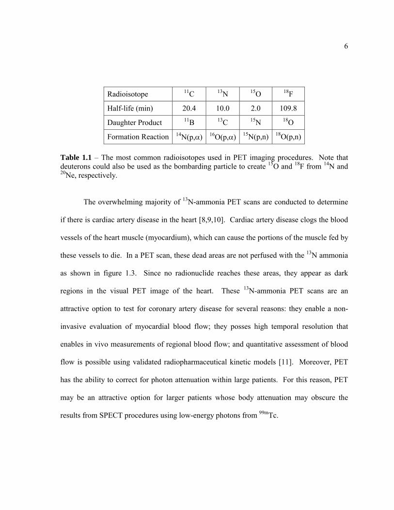
Section 1.3 The Use of 13N in PET Scans
As shown in table 1.1, 13N is one of several radioisotopes used in PET. Cyclotrons
are often used to produce this radioactive isotope of nitrogen from 16O(p,�)13N reactions in a
water target. The individually created 13N atoms bond with hydrogen to form 13NH3
ammonia molecules. The ammonia is separated from the water and injected into the
bloodstream of a patient. The typical activity of 13N-ammonia used for a PET scan is
approximately 20 mCi [8], and the high proton currents available in cyclotrons (~ 100 �A)
enable them to easily generate this 13N activity in water targets [2]. Although this is a rather
large initial activity, the 10-minute half-life results in a total dose to the patient that is
similar to that received from standard x-ray procedures.
6
Radioisotope 11C 13N 15O 18F
Half-life (min) 20.4 10.0 2.0 109.8
Daughter Product 11B 13C 15N 18O
Formation Reaction 14N(p,�) 16O(p,�) 15N(p,n) 18O(p,n) Table 1.1 – The most common radioisotopes used in PET imaging procedures. Note that deuterons could also be used as the bombarding particle to create 15O and 18F from 14N and 20Ne, respectively.
The overwhelming majority of 13N-ammonia PET scans are conducted to determine
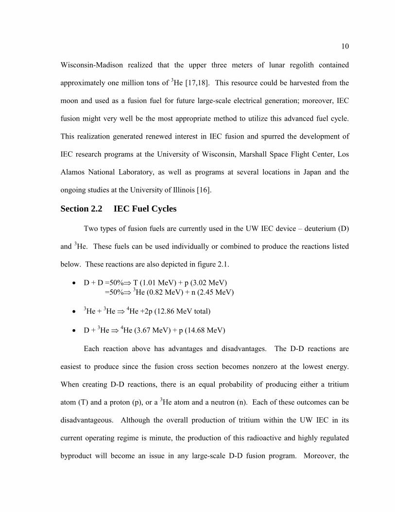
if there is cardiac artery disease in the heart [8,9,10]. Cardiac artery disease clogs the blood
vessels of the heart muscle (myocardium), which can cause the portions of the muscle fed by
these vessels to die. In a PET scan, these dead areas are not perfused with the 13N ammonia
as shown in figure 1.3. Since no radionuclide reaches these areas, they appear as dark
regions in the visual PET image of the heart. These 13N-ammonia PET scans are an
attractive option to test for coronary artery disease for several reasons: they enable a non-
invasive evaluation of myocardial blood flow; they posses high temporal resolution that
enables in vivo measurements of regional blood flow; and quantitative assessment of blood
flow is possible using validated radiopharmaceutical kinetic models [11]. Moreover, PET
has the ability to correct for photon attenuation within large patients. For this reason, PET
may be an attractive option for larger patients whose body attenuation may obscure the
results from SPECT procedures using low-energy photons from 99mTc.

7
Cross Sections for 16O(p,�)13N Reactions
0
40
80
120
160
200
5 7 9 11 13 15
Proton Energy (MeV)
Cro
ss S
ectio
n (m
b)
Figure 1.1 – Cross section for 16O(p,�)13N reactions. The 14.7 MeV protons generated from D-3He fusion are well suited to this reaction. This data was taken from IAEA’s charged particle cross section database for medical radioisotope production [1] at http://www-nds.iaea.or.at/medical/index.html.
8
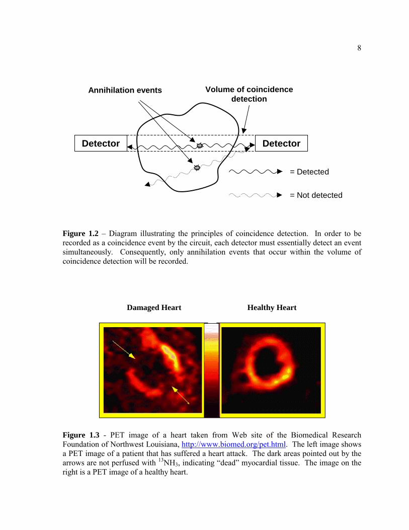
= Not detected
= Detected
Volume of coincidence detection
Annihilation events
Detector Detector
Figure 1.2 – Diagram illustrating the principles of coincidence detection. In order to be recorded as a coincidence event by the circuit, each detector must essentially detect an event simultaneously. Consequently, only annihilation events that occur within the volume of coincidence detection will be recorded.
Damaged Heart Healthy Heart
Figure 1.3 - PET image of a heart taken from Web site of the Biomedical Research Foundation of Northwest Louisiana, http://www.biomed.org/pet.html. The left image shows a PET image of a patient that has suffered a heart attack. The dark areas pointed out by the arrows are not perfused with 13NH3, indicating “dead” myocardial tissue. The image on the right is a PET image of a healthy heart.

9
Chapter 2 The University of Wisconsin Inertial Electrostatic Confinement Fusion Device
Section 2.1 Overview of Inertial Electrostatic Confinement Fusion
In the simplest terms, an inertial electrostatic confinement (IEC) fusion device is a
machine that uses large electrostatic potential differences to accelerate positive isotopic ions,
such as hydrogen or helium, into a central dense core region within a vacuum chamber. If
these ions have enough energy when they reach the dense core, there is a probability that
two ions will fuse together into a single atom, releasing particles and excess energy in the
process. Often designed for spherical symmetry, the ions that don’t fuse during their first
pass through the core may continue to oscillate within the electrostatic potential well and
fuse during later passes through the core. A portion of the ion population is continually
removed during operation by several loss mechanisms, including charge exchange reactions
with the background gas and collisions with the wires of the anode and cathode. However,
the practical simplicity, relatively small size and inexpensive cost make this type of fusion
attractive for many potential applications including isotope production, clandestine material
detection through neutron activation, and possibly even small power production devices.
Although a few IEC research programs, such as at the University of Illinois [12],
have been in place for several decades, few IEC fusion programs existed prior to the 1990s
[13-16]. At that time, IEC fusion seemed to have a very limited future. A discovery in
1987, however, re-ignited interest in IEC fusion and provided an opportunity for this little
talked about form of fusion to make its mark. In that year, researchers at the University of
10
Wisconsin-Madison realized that the upper three meters of lunar regolith contained
approximately one million tons of 3He [17,18]. This resource could be harvested from the
moon and used as a fusion fuel for future large-scale electrical generation; moreover, IEC
fusion might very well be the most appropriate method to utilize this advanced fuel cycle.
This realization generated renewed interest in IEC fusion and spurred the development of
IEC research programs at the University of Wisconsin, Marshall Space Flight Center, Los
Alamos National Laboratory, as well as programs at several locations in Japan and the
ongoing studies at the University of Illinois [16].
Section 2.2 IEC Fuel Cycles
Two types of fusion fuels are currently used in the UW IEC device – deuterium (D)
and 3He. These fuels can be used individually or combined to produce the reactions listed
below. These reactions are also depicted in figure 2.1.
�� D + D =50%� T (1.01 MeV) + p (3.02 MeV) =50%� 3He (0.82 MeV) + n (2.45 MeV)
��3He + 3He � 4He +2p (12.86 MeV total)
�� D + 3He � 4He (3.67 MeV) + p (14.68 MeV)
Each reaction above has advantages and disadvantages. The D-D reactions are
easiest to produce since the fusion cross section becomes nonzero at the lowest energy.
When creating D-D reactions, there is an equal probability of producing either a tritium
atom (T) and a proton (p), or a 3He atom and a neutron (n). Each of these outcomes can be
disadvantageous. Although the overall production of tritium within the UW IEC in its
current operating regime is minute, the production of this radioactive and highly regulated
byproduct will become an issue in any large-scale D-D fusion program. Moreover, the

11
production of tritium may indirectly cause some D-T reactions, which also produce
neutrons. The second reaction branch results in the direct production of fast neutrons, which
can damage the lattice structure of the containing vacuum chamber and cause it to become
radioactive. These neutrons will also interact with nearby equipment, potentially causing
further operational complications. These same neutrons could be put to useful purposes,
however; an IEC machine could be used to purposefully activate materials, such as those
within cargo containers or luggage, in an effort to detect clandestine items [19].
The 3He-3He fusion reaction is very advantageous since it does not produce any
radioactive products or neutrons. If this form of fusion can be achieved on a large scale (>
1015 reactions/sec), then a truly pollution-free source of energy may be attainable [20,21].
Unfortunately, the fusion cross section for 3He ions only becomes significant at very large
center-of-mass energies (applied potentials in excess of –200 kV). This has prevented the
demonstration of 3He fusion in any device to date. Significant research into this reaction is
ongoing at the University of Wisconsin, and a new chamber has been obtained solely for this
purpose.
The third fusion reaction, D-3He, has the very useful result of producing high-energy
protons. Burning deuterium and 3He in the IEC chamber does lead to D-D side reactions
and their associated neutrons; however, the reaction rate of each D-D reaction branch is
small enough at current operating regimes that the damage to and activation of materials is
negligible. This enables the high-energy protons from D-3He fusion reactions to be
beneficially exploited [22,23,24].
As stated, the goal of this proof-of-principle experiment is to produce 13N from the
oxygen atoms in a water target. However, the 14.7 MeV protons from D-3He fusion are
12
energetic enough to produce all of the PET isotopes listed in table 1.1. In fact, the cross
sections for the other reactions are even more favorable than those for 13N. Therefore,
isotope production may serve as an early application for IEC fusion devices en route to a
long-term goal of power production [22].
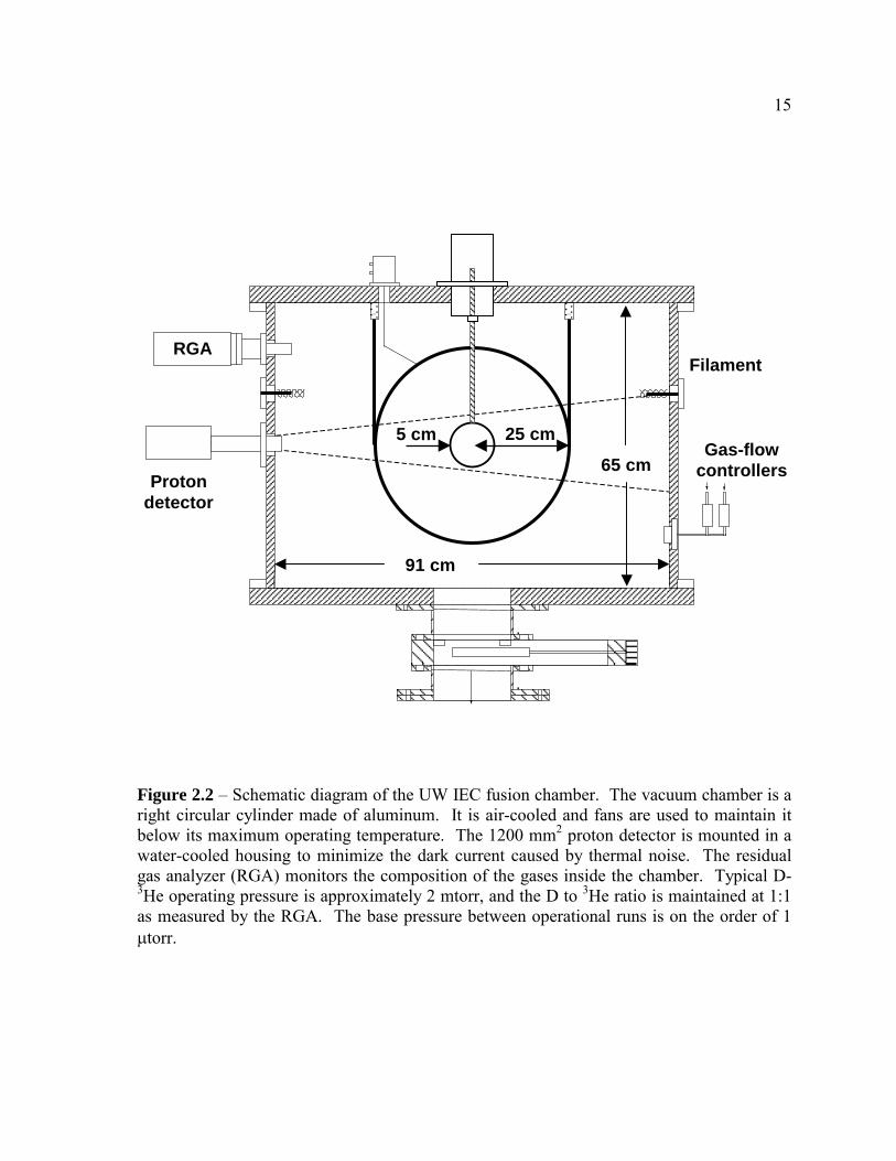
Section 2.3 The University of Wisconsin IEC Device
The UW IEC device is a two-grid, spherically symmetric IEC system contained
within an aluminum vacuum chamber that has the shape of a right circular cylinder. Figure
2.2 shows a schematic diagram of the device, and figure 2.3 shows a photograph of the
chamber while in operation at high pressures (~8 mtorr). The inside of the vacuum chamber
is 65 cm tall and 91 cm in diameter. The two grids of the IEC reside within this volume.
The outer grid, or anode, is made of stainless steel wires that are approximately 2 mm in
diameter. During operation, the anode is either maintained at zero potential via a grounding
connection or biased with a few hundred volts of negative potential. A large negative
potential is then applied to the inner grid, or cathode, which is fabricated from 0.8 mm
diameter tungsten-rhenium wire. For most UW applications, this negative potential ranges
from 40,000 to 160,000 volts, although operations to date have reached 180 kV.
This large negative voltage is generated by a Hipotronics™ DC power supply. The
supply is capable of producing up to 200,000 volts DC, either positive or negative, with up
to 75 mA of current. This electrostatic potential is transferred to the IEC chamber inside an
oil-filled feedthrough container, where it is carried to the cathode along a solid 0.32 cm
molybdenum rod. This rod is seated inside a 1.9 cm diameter boron-nitride stalk to prevent
the large voltage from shorting to the chamber walls and feedthrough. The cathode is
13
mounted directly to the molybdenum rod at the end of the stalk. When properly assembled,
the cathode is centered on the vertical and horizontal axis of the vacuum chamber.
A proton detector is mounted on the horizontal axis of the chamber to monitor the D-
3He reaction rate. This detector was a 1200 mm2, ion-implanted, surface barrier detector
from Ametek Industries, mounted 81 cm from the center of the cathode. The proton detector
only sees a small fraction of the total number of protons produced inside the IEC because is
it located at the end of a tube. This detection volume is approximated in figure 2.2
To ionize the gaseous fuel, three filaments from standard 200-watt light bulbs are
mounted equidistant from each other on the same plane of the vertical chamber walls. As
current is applied to the filaments, they become very hot and emit electrons via thermionic
emission. These electrons ionize a small fraction of the gaseous fuel within the chamber,
causing the now positive ions to be accelerated towards the cathode. The typical operating
pressure inside the chamber is approximately 2 mtorr, and the ratio of D to 3He is
maintained at 1:1 as measured by the residual gas analyzer (RGA).
The projected area of the solid cathode wires comprise only 8% of the surface area of
the cathode, so the cathode is 92% transparent to the ions. Theoretically, the spherical
geometry of the cathode causes the ions to converge at its center, creating a dense core of
ions. In reality, as much as 2/3’s of the D-3He fusion reactions are thought to occur as
embedded reactions approximately one micron deep in the cathode wires [25]. In either
event, the 14.7 MeV protons are isotropically emitted. Hence, the first challenge of this
experiment was to design a water containment system to intercept a portion of these protons
for 13N production.

14
50%
50%Tritium 1.01 MeV
3.02 MeVProton D
D 3He 0.82 MeV
Neutron 2.45 MeV
Proton3He
12.86 MeVTotal
3He 3He
Proton
4He 3.67 MeVD
14.68 MeVProton3He
Figure 2.1 – Fusion cycles used in the UW IEC chamber. No fusion device has yet been able to demonstrate 3He–3He fusion due to the very large electrostatic potentials (> 200 keV) required.
15
Proton detector
Filament
25 cm 5 cm Gas-flow
controllers
RGA
91 cm
65 cm
Figure 2.2 – Schematic diagram of the UW IEC fusion chamber. The vacuum chamber is a right circular cylinder made of aluminum. It is air-cooled and fans are used to maintain it below its maximum operating temperature. The 1200 mm2 proton detector is mounted in a water-cooled housing to minimize the dark current caused by thermal noise. The residual gas analyzer (RGA) monitors the composition of the gases inside the chamber. Typical D-3He operating pressure is approximately 2 mtorr, and the D to 3He ratio is maintained at 1:1 as measured by the RGA. The base pressure between operational runs is on the order of 1 �torr.

16
Figure 2.3 – The UW IEC chamber in operation using deuterium fuel at a pressure of approximately 8 mtorr.

17
Chapter 3 Design of Isotope Production System
Section 3.1 Separation of Radioisotope from Water Target
Shortly after deciding to create 13N using protons from D-3He fusion, a process was
devised that would allow the radioisotope to be separated from the water target in order to
efficiently measure its activity. Fortunately, separating 13N from its water environment is a
rather easy process. In this experiment, the 13N is created monotonically. If one can
manipulate the water environment such that the 13N atoms form a specific compound, these
compounds can easily be separated from the water through basic chemical processes. In
fact, the University of Wisconsin’s Medical Physics department uses this exact methodology
when they produce 13N for PET scans using a cyclotron. By preparing a water target that
contains approximately 10 millimolar of ethyl alcohol, the 13N atoms are driven to form
13NH3+ ammonia ions. These positive ions are then removed from the water target by
flowing the water through a column of ion exchange resin. Ion exchange resins are polymer
compounds possessing numerous ionic sites. Each site can reversibly exchange either
cations or anions (depending upon the resin) with similarly charged ions in the surrounding
solution. Thus, these resins trap compounds without altering their chemical properties [26].
For this experiment, DOWEX 50WX8 (100-200) cation exchange resin is used. The
DOWEX resin employs SO3� ions (covalently bound to the resin polymer) as ionic sites, and
H+ ions (ionically bound to the SO3�) as the vehicles for ion exchange. For this experiment,
the H+ atoms are replaced with Na+ ions by rinsing the resin in a solution of 0.1 molar
NaOH (see Chapter 5, Section 5.1). When the water containing the 13NH3+ ions is passed

18
through a column of DOWEX 50WX8 (100-200) resin, the resin exchanges its Na+ ions for
13NH3+ ions, thereby trapping the 13N in a volume small enough to measure its activity.
A second advantage of promoting the creation of 13NH3+ ammonia atoms is that this
is the form in which 13N is delivered to patients during a PET scan [8,9,10]. Before being
administered, the final solution of 13N ammonia must be sterilized, checked for chemical and
radionuclide purity, and so on. Since the chemical form of the 13N ammonia solution is the
same chemical form in which it will be administered to the patient, it eliminates the need for
intermediate chemical processes.
Section 3.2 Development of Experimental Apparatus
Once the water target was selected and the radioisotope separation method
determined, designing a comprehensive production system was straightforward. The system
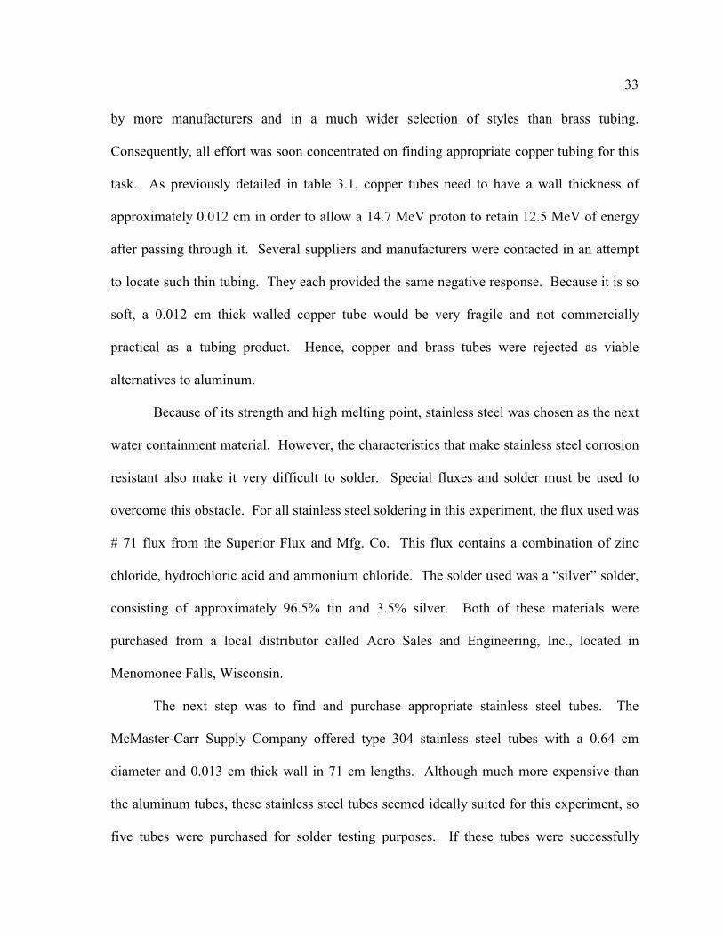
includes the following items:
1) A container placed inside the IEC to hold the water target.
2) A pump to circulate water through the closed system.
3) A heat exchanger to remove heat from the water. The IEC needs to operate in
excess of 140 kV and 30 mA during isotope production runs. These conditions
generate more than 4 kW of power inside the chamber, some of which will be
transferred to the water as heat. This heat must be removed to prevent the formation
of steam that could rupture the tubes and severely damage the vacuum pumps.
4) A water expansion reservoir which allows the volume of water to increase with
temperature. This reservoir also offers an escape for air trapped within the water
circuit.
5) An ion exchange column to separate the 13NH3+ from the water.

19
The above components are arranged in a closed loop isotope production system as shown in
figure 3.1. This circuit continually circulates the same volume of water through the water
containment apparatus within the IEC, where it is irradiated with protons.
The first and obvious challenge in developing a method for producing 13N from a
water target in an IEC chamber is how to contain the water. To efficiently produce isotopes,
the containment material must be thin enough to enable the protons to pass through with as
little energy loss as possible. Moreover, it has to be robust enough to withstand the internal
water pressure, the plasma environment, electron jets and the heat generated inside the IEC
chamber. Since it is used in a vacuum environment, the material can not significantly
outgas, nor can the products used to create joints and connections in the material.
With these characteristics in mind, thin-walled metallic tubing quickly becomes the
only viable alternative. Plastics were judged to be too sensitive to the plasma and electron
jets emanating from the plasma. It was also feared that the poor thermal conductivity of
plastic would not enable the water inside to cool a plastic container well enough to prevent
the development of leaks. Additionally, creating joints with plastic materials requires the
use of glues containing hydrocarbons, which may significantly outgas or react with the
plasma. Hence, plastic was eliminated as a possible water containment material. Glass was
also considered as a possibility, but the expense of creating a thin-walled glass structure, and
the inherent fragility of such a structure, lead to its rejection. Finally, some initial research
concluded that ceramics, carbon fiber objects and other exotic materials would be either too
expensive, too difficult to work with or both. As a result, thin-walled metallic tubing
became the design material for a water containment apparatus.

20
The more energy the protons enter the water target with, the larger the yield of 13N
will be. In order to enable a proton to pass through it and retain a significant fraction of its
original energy, the wall of a metallic tube would need to be very thin indeed. Hence, initial
planning and design efforts focused on finding metallic tubing of a thickness such that the
incident protons only lost approximately 2 MeV in traveling through the tube wall. This
results in the proton entering the water target with approximately 12.5 MeV of energy.
To determine the wall thickness that would enable the protons to retain 12.5 MeV of
energy (assuming they are incident normal to the tube wall), the range and stopping powers
of several materials were investigated. Figure 3.2 plots the continual slowing down
approximation (CSDA) range of protons in aluminum, stainless steel and water [27]. The
range of protons in copper was also examined and found to be so similar to stainless steel
that the two could not be differentiated when plotted together in figure 3.2. Consequently, it
was not included in the graph. Figure 3.2 clearly demonstrates that a 15 MeV proton has
more than twice the range in aluminum than in stainless steel (or copper).
Comparing the stopping powers of these materials for a 14.7 MeV proton also
demonstrates the advantage of aluminum. Table 3.1 lists the stopping power for 14.7 MeV
protons in the three materials, and the thickness of material that would attenuate a 14.7 MeV
proton to 12.5 MeV. This table demonstrates that aluminum tubes could have a wall
thickness more than twice that of copper or stainless steel tubes for the same proton energy
degradation. This fact proved to be an advantage since tubes with a wall thickness as small
as 0.012 cm are difficult to procure.

21
Al Cu SS Stopping Power (MeV /cm) 67.66 181.97 172.23
Wall thickness to slow a proton to 12.5 MeV (cm) 0.0325 0.0121 0.0127
Table 3.1 – Stopping power of various metallic tubing materials and the wall thickness required to slow a 14.7 MeV proton to 12.5 MeV [27].
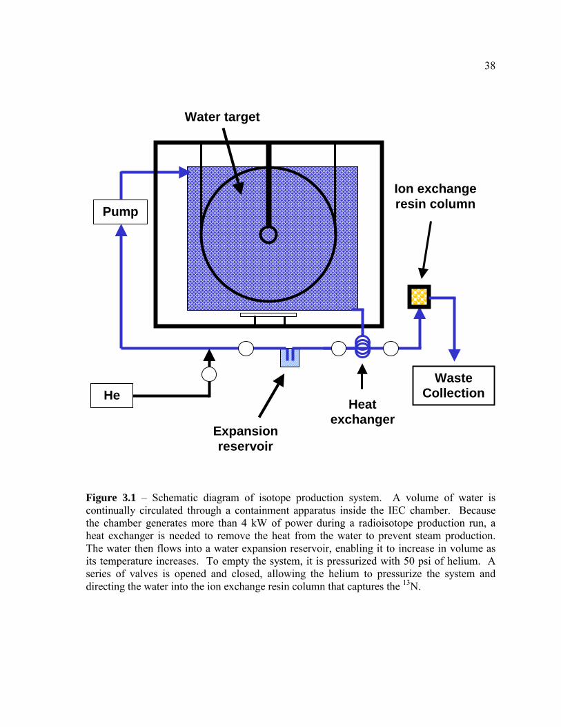
In an attempt to create a simple and adaptable water containment apparatus, initial
designs focused on using coils of thin-walled tubing. One design called for a spiral target
that expanded out from a central water inlet much like an old fashioned children’s lollipop
(figure 3.3). This target could be placed at the bottom of the chamber under the anode and
would intercept a significant portion of the protons produced. A second design (figure 3.4)
specified a coil of tubing that would wind around the inner wall of the IEC chamber. If the
coil covered the height of the IEC chamber wall from top to bottom, this target would
intercept an even larger fraction of the protons produced. Both designs had the benefit of
having only two connections – one on each end of the coil of tube. Fewer connections
obviously reduces the opportunity for leaks to develop at such junctions. Unfortunately, no
commercially manufactured coiled tubing could be found with walls thin enough for this
experiment. Several manufacturers contacted in regard to this coiled tubing stated that such
thin walled tubing was too susceptible to kinking during handling to be a practical
commodity. Therefore, these designs were rejected. If a manufacturer could be found that
would make a coil of thin walled tubing, it’s believed these would be very successful
designs.
After further deliberation, a design was selected that incorporated numerous tubes
closely aligned alongside each other and connected by manifolds at either end. As shown in

22
figure 3.5, this design was very similar to a car radiator; hence, “the radiator” became its
unofficial nickname. Water would flow in one end of a manifold, be distributed among the
approximately 65 tubes, and then flow out the opposite end of the second manifold. The
flow was directed in and out of the “radiator” at opposite corners in order to encourage an
even flow of water through each tube. If sized appropriately (about 60 cm x 60 cm), this
design can either be placed vertically in the IEC chamber between the anode and the
chamber wall, or horizontally between the anode and chamber floor. Assuming an isotropic
distribution of protons from a point source in the center of the cathode, neither location
provides an advantage in terms of the proton flux. There was some concern that a horizontal
orientation might inhibit the outflow of gas through the turbo-pump at the bottom of the
chamber, but later experiments with this orientation did not demonstrate any pumping
restrictions.
Although feasible, this design does have some apparent drawbacks. One concern is
that the flow will not be equally distributed, causing the flow in some tubes to be very slow
relative to the others. The water in these tubes might then become hot enough to turn to
steam and rupture the system. It was felt that this could be overcome by moderating the
flow rate to ensure adequate flow through all tubes, though. Later experiments
demonstrated that a total flow rate of approximately one liter per minute provided adequate
flow through all the tubes. Another concern with this system is the significant number of
joints needed to fabricate this design. Incorporating approximately 65 tubes necessitates 130
joints – two for each tube. Not only does this increase the effort required to fabricate the
apparatus, but these numerous joints may also be a potential source of leaks. This concern
was eventually realized.

23
Section 3.3 The Model ALM1 Water Containment Apparatus
As previously described, aluminum tubing of wall thickness 0.0325 cm reduces the
energy of a 14.7 MeV proton to approximately 12.5 MeV. Moreover, aluminum tubing is
readily available and relatively inexpensive. Hence, the first isotope production system was
built using aluminum tubes as the foundation of the water containment apparatus. Because
it was fabricated from aluminum tubing and was the first model built, this system was
designated the Model ALM1.
The first step in constructing the Model ALM1 apparatus was to obtain the
appropriate tubes. Since the range of a 12.5 MeV proton in water is less than 0.2 cm, the
diameter of the tubes in the Model ALM1 did not need to be very large. For simplicity of
handling and adequate flow capability, however, ¼ inch (0.635 cm) nominal diameter
aluminum tubes were selected. These tubes were purchased from the McMaster-Carr
Supply Company of Chicago, Illinois. Each type 3003 alloy aluminum tube was two-meters
in length and 0.64 cm in diameter with a wall thickness of 0.036 cm. These tubes reduce the
energy of a 14.7 MeV proton to approximately 12.3 MeV.
The two-meter long sections of aluminum tubing were cut to 58 cm lengths by hand
using standard pipe cutters. These cutters severed the tubes cleanly, but care had to be taken
to prevent crushing the tubes by applying too much force with the cutting wheel. Once cut,
the inside of the tubes were cleaned in a four-step process. First, the tubes were cleaned in
hot soapy water using a 223 caliber rifle cleaning kit with copper bore brush. Each tube was
cleaned just as if it were the bore of a rifle. After this was done, the tubes were cleaned in a
similar manner using hot water only. This was done to rinse away the soap. The tubes were

24
then blown dry using compressed air and rinsed with acetone to remove any remaining
traces of grease. Finally, the tubes were rinsed with alcohol to remove the acetone.
The last step in preparing the tubes was to flatten their middle portions. This was
done to provide a flat tube face to the protons incident perpendicularly to the tube’s
projected area. By having a flat face instead of a round face, the wall thickness across the
entire width of the tube would be uniform (see Chapter 4, Section 4.4, Paragraph 5 for
further discussion of this effect). The ends of each tube were not flattened in order to ensure
their original round geometry would fit tightly into the round holes drilled in the manifolds.
Flattening the middle portion of each tube was accomplished using two large metal
bars approximately 10 cm wide, 2.5 cm thick and 45 cm long. Six washers were glued onto
the face of one bar to prevent the face of the second bar from getting closer than about 0.4
cm to the face of the first. Additionally, the edges of each end of the bars were rounded to
provide a smooth transition from the flattened portion of the tube to the round end (see
figure 3.6). A tube was placed on the bar with the washers, and the second bar was placed
on top of the tube sandwiching it between the bars. The bars were then placed in a press and
the top bar was forced down upon the bottom bar, flattening the tube to a thickness of
approximately 0.4 cm in the process.
After flattening several tubes in this manner, it was observed that this process caused
the tubes to take on a “figure 8” shape; the tubes were rounded on the edges with a crease
down the middle of both sides. To flatten the face of the tubes as intended, each tube was
slightly expanded by pressurizing it to approximately 100 psi. This was accomplished by
capping one end of a tube with a Swageloc™ fitting, and using a similar fitting on the other
end to connect it to the regulator of a high-pressure nitrogen tank. This caused the tubes to
25
take on a “pointed oval” shape much like a cat eye. Although requiring considerable time
and effort, the final tube shape presented a much more consistent wall thickness to incident
protons than the original round shape.
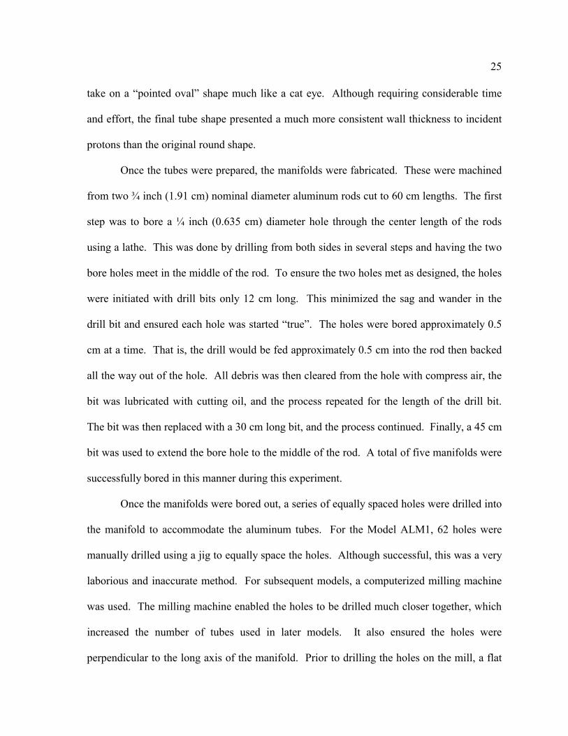
Once the tubes were prepared, the manifolds were fabricated. These were machined
from two ¾ inch (1.91 cm) nominal diameter aluminum rods cut to 60 cm lengths. The first
step was to bore a ¼ inch (0.635 cm) diameter hole through the center length of the rods
using a lathe. This was done by drilling from both sides in several steps and having the two
bore holes meet in the middle of the rod. To ensure the two holes met as designed, the holes
were initiated with drill bits only 12 cm long. This minimized the sag and wander in the
drill bit and ensured each hole was started “true”. The holes were bored approximately 0.5
cm at a time. That is, the drill would be fed approximately 0.5 cm into the rod then backed
all the way out of the hole. All debris was then cleared from the hole with compress air, the
bit was lubricated with cutting oil, and the process repeated for the length of the drill bit.
The bit was then replaced with a 30 cm long bit, and the process continued. Finally, a 45 cm
bit was used to extend the bore hole to the middle of the rod. A total of five manifolds were
successfully bored in this manner during this experiment.
Once the manifolds were bored out, a series of equally spaced holes were drilled into
the manifold to accommodate the aluminum tubes. For the Model ALM1, 62 holes were
manually drilled using a jig to equally space the holes. Although successful, this was a very
laborious and inaccurate method. For subsequent models, a computerized milling machine
was used. The milling machine enabled the holes to be drilled much closer together, which
increased the number of tubes used in later models. It also ensured the holes were
perpendicular to the long axis of the manifold. Prior to drilling the holes on the mill, a flat

26
surface approximately 0.5 cm wide was milled into the round tube. This flat surface
prevented the drill bit from wandering across the round face of the rod and further improved
the precision of the process. The last step in fabricating the manifold was to enlarge the hole
through the rod at each end to a depth of 2 cm to accommodate Swageloc™ fittings. The
associated plumbing that brought the water into and out of the vacuum chamber was
connected to these fittings.
After the manifolds were fabricated, the apparatus was assembled. Creating a leak-
tight joint between aluminum components is, in general, a difficult task. It’s commonly
known that aluminum is very difficult to solder. Soldering the joints together was
investigated, though, to determine if it could be done reliably and repetitively. After
consulting many local welding, plumbing and metal supply companies, it became clear that
soldering aluminum was far too difficult to be relied upon for so many joints. Therefore, the
joints between the aluminum tubes and the manifolds were sealed using a special epoxy
manufactured by Varian Vacuum Technologies.
Named Torr Seal™, it’s a sealant designed specifically for high vacuum applications
and is a two-part epoxy comprised of a resin base and hardener. The two components come
in separate tubes and are mixed together to form the sealing compound. After preparing this
sealant for the Model ALM1 apparatus, the epoxy was heated with a heat gun set to
approximately 200o C. The heating served two purposes. First, when warmed the epoxy
became much thinner in consistency. This aided in spreading and filling the voids of each
joint. This consistency did not last long, however, so several small batches were made
during the assembly process. Second, the Torr Seal™ hardens much faster after its been
heated, enabling the apparatus to be assembled more quickly.

27
Before preparing the epoxy, a manifold was secured in a vice with the series of holes
in its side facing up. A wooden dowel was then placed in the bore of the manifold to
support the tubes as they were inserted into their respective hole. The dowel also assured
that the tubes were not placed too far into their holes, thereby restricting the water flow
through the manifold. Once the epoxy was mixed and heated, it was spread thinly over one
end of a tube. The tube was then inserted into an appropriate hole, then rotated, slightly
withdrawn and reinserted until it rested on the wooden dowel. The process served to
distribute the epoxy through the joint and was found to create the best possible seal. In this
manner, each tube was individually glued into place in one manifold as shown in figure 3.7.
The Torr Seal™ was then allowed to fully harden before completing the assembly.
In order to complete the assembly of the second manifold, a wooden frame was used
to secure the manifolds at the exact distance they needed to be from one another once
assembled. Having been flattened, the ribbon-like tubes were very flexible. Once the
remaining free end of an individual tube was coated in Torr Seal™, the tube was easily
bowed and its end inserted into the second manifold. Since the opposite end of each tube
was already glued into the first manifold, the tubes could not be rotated in order to distribute
the epoxy. If needed, a cotton swab was used to distribute the Torr Seal™ around each joint
to form a thick meniscus of epoxy. Once all tubes were glued into the two manifolds, the
Swageloc™ fittings were sealed in place with Torr Seal™ in a manner similar to that
described for the tubes. After the Torr Seal™ had cured for 24 hours, the Model ALM1
apparatus was placed under vacuum to check the integrity of the joints. Not unexpectedly,
some joints did have leaks. Pressurizing the system and placing it underwater exposed these
immediately; the leaks were easily spotted by the trail of bubbles emanating from them. The

28
leaks were patched with additional Torr Seal™. Prior to placing the Torr Seal™ on the
leaking joint, the ALM1 apparatus was placed under vacuum so that the epoxy would be
drawn into the leak and form a better patch. This method worked very well to patch all
leaks. The completely assembled Model ALM1 apparatus is shown in figure 3.8.
While the Model ALM1 apparatus was under construction, the associated plumbing
to support the apparatus was installed on the chamber. Since this plumbing only served to
carry the water to the ALM1 apparatus and did not play a role in isotope production (did not
need to allow protons to penetrate), it could be made from any material. Two lengths of
copper tubing were used to transport the water in and out of the IEC chamber. This was
done by inserting the copper tube through Swageloc™ fittings threaded into holes of a plate
on the bottom of the chamber as shown in figure 3.9. The Swageloc™ fittings created an
airtight seal around the copper tubes through the use of ferrules. The exterior ends of the
two copper tubes were capped with valves as shown in figure 3.10. Swageloc™ fittings
were placed on the interior ends of the two copper tubes; these fittings would join with those
cemented into the manifolds, thereby connecting the Model ALM1 apparatus inside the
chamber to the outside environment. Figure 3.11 shows the Model ALM1 apparatus
installed in the UW IEC chamber.
As it turns out, the Model ALM1 apparatus developed numerous leaks and could not
be made to work. The best operating conditions achieved were 90 kV and 30 mA. Initially,
the leaks developed at the joints that were cemented with Torr Seal™. These leaks
developed after only a few conditioning runs in the chamber. The water leak was detected
by a significant peak on the residual gas analyzer (RGA) at an atomic weight of 18. The
apparatus was immediately removed and its interior dried. It was then pressurized to locate
29
the leaks (there was no visible evidence of the leaks), then placed under vacuum to patch the
leaks with Torr Seal™. This process repeated itself until the radiator could be proven to be
leak-tight under vacuum and under pressure. The apparatus was then placed back in the
chamber and a series of conditions runs with the IEC were conducted. Invariably, more
leaks would develop and the repair process would begin again. During the conditioning
runs, the water within the apparatus would approach 60o C as measured with a thermocouple
attached to the copper tube carrying water out of the chamber. It was assumed that these
leaks developed due to differences in thermal expansion between the aluminum and the
epoxy. To prevent this from happening, the joints were thermally stressed by heating the
aluminum manifold to 100o C. This did create more leaks, which were then patched. This
process was repeated until the heating did not cause additional leaks. The apparatus was
then placed into the IEC.
During the conditioning runs following the reinstallation of the Model ALM1
apparatus, there was an occasion to operate at high chamber pressure (> 6 mtorr). Water had
not yet been introduced into the isotope production system, but it was filled with air at
atmospheric pressure. It’s not uncommon for electron jets – concentrated beams of
electrons emitted from the cathode – to be observed in the chamber during high-pressure
runs. These jets were known to crack the protective glass coverings of the observation ports
and even to melt the stainless steel wires of the anode. Their destructive power became all
too apparent, though, when a jet was incident upon the ALM1 apparatus during the high
pressure run.
After only a few minutes of operation, an enormous air leaked developed within the
chamber. After shutting down the experiment, a visual inspection of the ALM1 apparatus
30
from an observation port indicated a hole had been burned through a tube in the apparatus.
The apparatus was removed from the chamber and the full extent of the damage was clear.
As shown in figure 3.12, an electron jet burned holes in two tubes adjacent to each other,
and heated a third tube to such an extent that it was permanently warped from the heat.
These tubes were quickly replaced and the chamber was never again operated at high
pressure with the water containment apparatus inside.
Shortly after the ALM1 apparatus was repaired and installed, a series of conditioning
runs were conducted to determine if the chamber could successfully operate at high voltages
with the ALM1 inside. Unfortunately, the apparatus developed leaks almost immediately.
But unlike before, these leaks occurred near the edges of the flattened aluminum tubes and
not in the joints. It’s thought that these leaks were caused by stress fractures induced during
the tube-flattening processes. It’s unclear, however, why these leaks did not express
themselves immediately during the initial leak checks or the previous operational runs.
The leaks on the aluminum tubes were patched using Torr Seal™ in a manner similar
to sealing the joints. When the epoxy was hardened, these areas were wrapped in aluminum
to minimize any interaction between the epoxy and the plasma. Once proven leak-tight
under vacuum using sensitive vacuum gauges and even a helium leak checker, the ALM1
apparatus was placed back into the chamber for a final round of operational tests. After only
a few runs, however, the ALM1 apparatus developed more leaks near the edges of the
flattened aluminum tubes. It was concluded that these “stress” leaks would continue to
develop and that a new apparatus would need to be constructed to resolve the problem.

31
Section 3.4 The Model ALM2 Water Containment Apparatus
The second series of leaks in the Model ALM1 apparatus all developed at the edge of
the aluminum tubes and not in the joints; therefore, it was believed that another water
containment apparatus could be constructed from round (not flattened) aluminum tubes
using Torr Seal™ by thermally stressing the joints.
If the Model ALM1 apparatus could be described as a one panel assembly, then the
Model ALM2 apparatus was a two panel assembly. As shown in figure 3.13, it consisted of
two rows of aluminum tubes mounted perpendicularly to each other in one central manifold,
and two other manifolds mounted on each of the two sets of tubes. This L-shaped assembly
was designed to be placed inside the IEC chamber with one panel in the horizontal plane
below the anode, and the other panel vertically situated between the anode and the chamber
wall. The angle between the two panels was actually slightly more than 90 degrees so that
water would drain to the outer end of the horizontal panel when the vertical panel was
placed at 90 degrees to the chamber floor.
The tubes and manifolds used in the Model ALM2 apparatus were constructed from
the same materials and in the same manner as the ALM1. The joints were sealed with
heated Torr Seal™ as before, and the round tubes were bowed in order to insert them into
the manifolds just as the flattened tubes were. Although the round tubes were not nearly as
flexible as the flattened tubes, the did have enough give to enable them to be bowed and
inserted between two manifolds that were fixed in placed by a wooden frame. The
Swageloc™ fittings were placed in one corner of the vertical panel and in the opposite
corner of the horizontal panel to promote an equal distribution of water flow through all
tubes.

32
When the ALM2 was fully assembled and the epoxy fully cured, the manifolds were
heated to 100o C to thermally stress the epoxy joints. This created numerous leaks in the
joints, but these were easily found and patched. The heating and patching process continued
until no additional leaks were detected. The apparatus was then mounted inside the IEC
chamber, connected to the copper plumbing, and the system filled with water.
After only a few conditioning runs, the ALM2 apparatus developed leaks. After the
apparatus was removed from the IEC chamber, it was determined that the epoxy joints were
leaking. The ALM2 was placed under vacuum and the joints were patched with heated Torr
Seal™. The apparatus was thermally stressed and more leaks were found. This process
continued until the ALM2 was proven leak-tight. It was then placed back into the chamber
for another operational test. Unfortunately, the system again developed leaks after only a
few runs at 80 kV and 30 mA. It seemed as if there were more to the failure of the epoxy
joints than just differences in thermal expansion. Although there was no evidence to
indicate the specific cause of the leaks, it was assumed that the plasma somehow contributed
to the failures and that this problem would not be overcome. Therefore, the Model ALM2
was retired and a new, more robust system was designed.
Section 3.5 Stainless Steel Water Containment Apparatus
The experience with the ALM1 and ALM2 apparatus demonstrate that the joints of
any water containment apparatus need to be as rugged as the tubes themselves. This seemed
to necessitate soldering the joints between the tubes and the manifolds. Aluminum was
determined to be far too difficult to solder successfully, so another tube material would need
to be substituted for aluminum. Copper and brass are very easy to solder and, therefore,
were the first metals investigated. Due to its innumerable uses, copper tubing is fabricated
33
by more manufacturers and in a much wider selection of styles than brass tubing.
Consequently, all effort was soon concentrated on finding appropriate copper tubing for this
task. As previously detailed in table 3.1, copper tubes need to have a wall thickness of
approximately 0.012 cm in order to allow a 14.7 MeV proton to retain 12.5 MeV of energy
after passing through it. Several suppliers and manufacturers were contacted in an attempt
to locate such thin tubing. They each provided the same negative response. Because it is so
soft, a 0.012 cm thick walled copper tube would be very fragile and not commercially
practical as a tubing product. Hence, copper and brass tubes were rejected as viable
alternatives to aluminum.
Because of its strength and high melting point, stainless steel was chosen as the next
water containment material. However, the characteristics that make stainless steel corrosion
resistant also make it very difficult to solder. Special fluxes and solder must be used to
overcome this obstacle. For all stainless steel soldering in this experiment, the flux used was
# 71 flux from the Superior Flux and Mfg. Co. This flux contains a combination of zinc
chloride, hydrochloric acid and ammonium chloride. The solder used was a “silver” solder,
consisting of approximately 96.5% tin and 3.5% silver. Both of these materials were
purchased from a local distributor called Acro Sales and Engineering, Inc., located in
Menomonee Falls, Wisconsin.
The next step was to find and purchase appropriate stainless steel tubes. The
McMaster-Carr Supply Company offered type 304 stainless steel tubes with a 0.64 cm
diameter and 0.013 cm thick wall in 71 cm lengths. Although much more expensive than
the aluminum tubes, these stainless steel tubes seemed ideally suited for this experiment, so
five tubes were purchased for solder testing purposes. If these tubes were successfully

34
soldered to a stainless steel manifold, then a new water containment apparatus would be
constructed from them.
The five stainless steel tubes were each manually cut into four equal lengths using a
small tube cutter. This was much more difficult than anticipated, and it quickly became
apparent that a more robust mechanical method would be needed to cut the large number of
tubes required for a water containment apparatus. A small length of stainless steel tube 1.91
cm in diameter with a wall thickness of 0.32 cm was used to simulate the manifold. Ten
0.64 cm diameter holes were drilled into this tube approximately 0.5 cm apart. Flux was
liberally applied to each hole and to one end of several tubes. Each tube was then inserted
into a hole, and a small oxy-acetylene torch was used to heat the manifold. The thin-walled
tubing heated very quickly and great care had to be taken not to burn a hole through them.
The torch flame was directed at the manifold approximately one centimeter from the joint.
When hot enough, solder was applied to the joints. Because of the poor conductivity of the
stainless steel, the area around each joint had to be heated independently. Moreover, both
sides of the manifold tube had to be heated. All the while, flux was constantly applied to the
joint to ensure the solder bonded to the stainless steel. This process became a juggling act
and it was very difficult to solder the ten tubes, although it was done successfully.
To simplify the soldering process and better control the manifold temperature, an
electrical circuit was employed to heat a second test manifold much like the burner of an
electric stove. A large, 220 volt variable step-down transformer was used to induce a
current in a heavy copper wire attached to each end of the manifold as shown in figure 3.14.
This 4/0 gauge wire was looped through the transformer five times. Solid copper clamps
located at the ends of the wire attached to the manifold much like the terminals of a car

35
battery. When powered, the transformer could be adjusted to control the current through,
and therefore the temperature of, the stainless steel manifold. The resistance of the stainless
steel caused the manifold to quickly heat to temperatures in excess of 230o C, the melting
point of the solder. This technique worked very well and was quite simple. The only
drawback was the enormous cloud of corrosive steam created as the liberally applied flux
began to boil. A tremendous amount of ventilation was needed to control this. Moreover, a
mask, rubber gloves and goggles (not just protective glasses) were needed to prevent the
steam from irritating the nose, throat, hands and eyes.
Once a method was developed and successfully tested to solder together a stainless
steel apparatus, the materials necessary to build the Model SSM1 were obtained. Located in
the glass shop of the UW physics department, a table saw with corundum blade was used to
cut the 70 tubes necessary for the SSM1 design. This was a very fast and efficient process.
A jig ensured each tube was cut to the specified length with millimeter accuracy. Once cut,
the tubes were cleaned in the same four-step manner as the aluminum tubes. The two
stainless steel manifolds did not need to be bored out like the aluminum manifolds, since
they were fabricated from tubing and not bar stock. The computerized milling machine was
used to drill the 70 holes along the length of the tube as previously discussed. These were
drilled using a ¼ inch titanium nitride-tipped drill bit. The ¼ inch nominal diameter tubes
fit snugly into these holes – so snugly, in fact, that when dry-assembled it was rather
difficult to take it apart.
Immediately prior to assembly, each hole in the manifolds and each end of the tubes
were coated with flux. The Model SSM1 apparatus was then pieced together entirely and
the inductive heating circuit was connected to one manifold. The joints were brushed with

36
flux one last time as the transformer began heating the manifold. The ends of the manifold
heated the fastest and reached the highest temperature. When the temperature at the center
of the manifold was hot enough to melt the solder, the transformer was shut off and the
solder wire was run along the manifold across the joints at a quick and steady pace. Only
two passes were made with the solder; it was run up one side of the joints and down the
other. The manifold was visually examined to locate any joints that did not have a meniscus
of solder around the base of its tube. The solder was quickly touched to those areas, and
then the manifold was misted with water to cool it below 230o C and lock the tubes in place.
The copper electrodes were then removed from one manifold and connected to the other.
The same soldering process was employed, and in a matter of minutes all 140 joints were
soldered.
The boiling flux left a thick, tar-like residue on both the inside and outside of the
tubes. This had to be removed in order to minimize the ions released into the water that
would eventually circulated through the apparatus. Before the Swageloc™ fittings were
soldered to the manifolds, the inside and outside of the Model SSM1 was thoroughly rinsed
with an industrial toilet bowl cleaner called Solvit™, which contains 24% hydrochloric acid.
This cleaner quickly removed the residue from the outside of the apparatus, and it appeared
to remove it from the inside as well. Immediately after flushing the bowl cleaner from the
apparatus, it was rinsed repeatedly with hot soapy water. It was then rinsed with hot water,
then acetone and finally alcohol.
After this thorough cleaning, the Swageloc™ fittings were soldered into both ends of
each manifold. This was a slight difference from the Model ALM1 and ALM2 apparatus. It
was done to provide more flexibility for the associated plumbing, and to allow the SSM1 to

37
be connected in series at a later date with similar, additional apparatus if need be. With the
fittings in place, the SSM1 was put under vacuum to test the integrity of the soldered joints.
Surprisingly, this test indicated that many of the tubes themselves each contained numerous
pinholes. After speaking with both the manufacturer and the supplier, it was learned that
this batch of tubes had been improperly manufactured. The manufacturer agreed to
immediately fabricate a new batch of tubes for the experiment.
When the new batch of tubes arrived, they were checked for leaks using a helium
leak checker. No tube from this batch contained a leak. Hence, the Model SSM2 apparatus
was immediately constructed. The cutting, cleaning, soldering and leak checking methods
used for the SSM2 were identical to those described for the SSM1. When the SSM2 was
fully assembled and check for leaks, a few leaks were found in the soldered joints. These
joints were heated with two heat guns from opposing angles and soaked with flux. After a
few minutes of heating by the guns, the area around the joint was hot enough to melt the
solder. The liquid solder was then teased around the joint with a length of stainless steel
wire. This helped ensure a complete meniscus around the tube joint. Unlike patching leaks
in the Models ALM1 and ALM2 apparatus, the SSM2 was not placed under vacuum when
patching its leaks with solder. This is because the molten solder is much more viscous then
the Torr Seal™, and would be drawn completely through the hole without patching it.
Figures 3.15 contain a picture of the fully assembled SSM2 apparatus.
The SSM2 water containment apparatus proved to be a very rugged and successful
design. The IEC was operated at potentials reaching 155 kV, and at lower voltages with
currents of 60 mA, with the apparatus inside. It developed only one minor leak during its
operational lifetime, and that was easily repaired.
38
Water target
Expansion reservoir
He Waste
CollectionHeat
exchanger
Pump
Ion exchange resin column
Figure 3.1 – Schematic diagram of isotope production system. A volume of water is continually circulated through a containment apparatus inside the IEC chamber. Because the chamber generates more than 4 kW of power during a radioisotope production run, a heat exchanger is needed to remove the heat from the water to prevent steam production. The water then flows into a water expansion reservoir, enabling it to increase in volume as its temperature increases. To empty the system, it is pressurized with 50 psi of helium. A series of valves is opened and closed, allowing the helium to pressurize the system and directing the water into the ion exchange resin column that captures the 13N.

39
Proton Energy vs. Range in Aluminum, Stainless Steel & Water
0
500
1000
1500
2000
2500
3000
0 2 4 6 8 10 12 14 16
Proton Energy (MeV)
CSD
A R
ange
( �m
)
Water Aluminum Stainless Steel
Figure 3.2 – Graph of CSDA range vs. proton energy in three materials. The range of protons in copper is very similar to their range in stainless steel. As this graph shows, protons have more than twice the range in aluminum than in stainless steel. This means that an aluminum tube could have more than twice the wall thickness of a stainless steel (or copper) tube for a given proton energy loss in the tube wall.

40
Water outletWater inlet
FigureThis isthe charejectedrequire
Cathode
3.3 – Schematic diagram of spiraling coil design for water containment apparatus. a top view of the UW IEC chamber. The spiral target would rest on the bottom of mber. Water would flow in one end of the spiral and out the other. This design was , however, since no coiled tubing could be found with walls thin enough to meet our
ments.
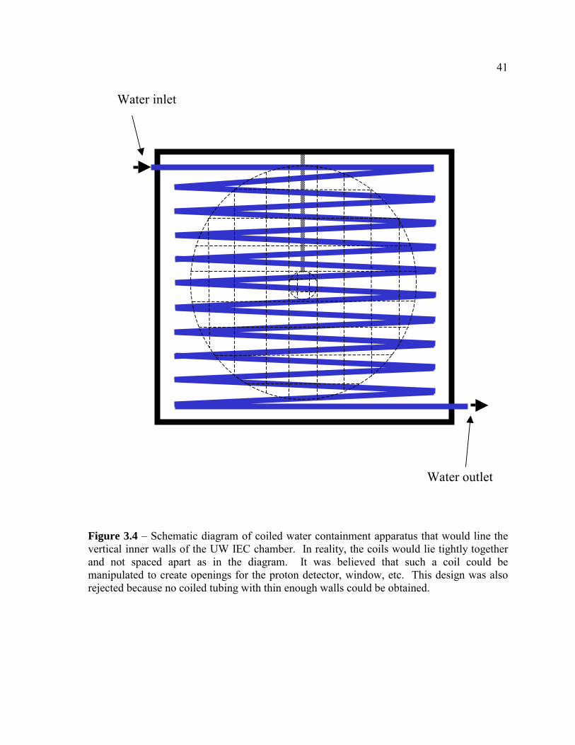
41
Water outlet
Water inlet
Figure 3.4 – Schematic diagram of coiled water containment apparatus that would line the vertical inner walls of the UW IEC chamber. In reality, the coils would lie tightly together and not spaced apart as in the diagram. It was believed that such a coil could be manipulated to create openings for the proton detector, window, etc. This design was also rejected because no coiled tubing with thin enough walls could be obtained.
42
Manifolds
Front View Side View
Figure 3.5 – The “radiator” design incorporating approximately 65 vertical tubes closely aligned alongside each other. A manifold at either end enabled water to be distributed through and collected from each tube.

43
Washers
Rounded edge
Tube to be flattened
10 cm
45 cm
Side View Top View
Figure 3.6 – Schematic diagram of one bar used to flatten the central portion of the aluminum tubes in the Model ALM1 apparatus. A tube was place on this bar, and a press was used to force an identical bar down on top of it. This flattened the aluminum tube between the bars to a thickness of approximately 0.4 cm. The washers glued to one bar prevented the tube from being completely flattened.

44
Torr Seal joints
Figure 3.7 – Model ALM1 apparatus under construction. The joints between the flattened tubes and the manifold were sealed using Torr Seal™, an epoxy by Varian Vacuum Technologies designed specifically for high vacuum environments.

45
Figure 3.8 – Picture of the Model ALM1 water containment apparatus. Note that the vertical tubes have been flattened to present a constant wall thickness to incoming protons.

46
Figure 3.9 – Photograph of plate through which the copper plumbing of the isotope production system passes. The copper tubes are fed through Swageloc™ fittings, which are screwed into the plate and their threads sealed with Torr Seal™. The fittings fix the copper tubes in place and provide a leak-tight seal.

47
Valves
Swageloc fittings
Figure 3.10 – Exterior view of copper plumbing exiting the chamber through Swageloc™ fittings. The ends of the tubes are capped with a valve that controls the flow in and out of the water containment apparatus.
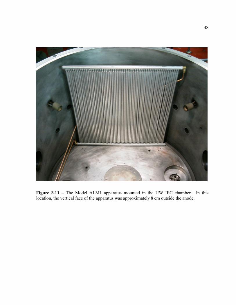
48
Figure 3.11 – The Model ALM1 apparatus mounted in the UW IEC chamber. In this location, the vertical face of the apparatus was approximately 8 cm outside the anode.
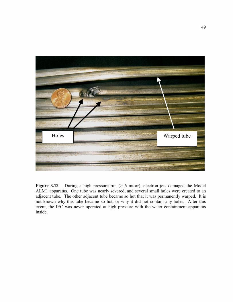
49
Warped tube Holes
Figure 3.12 – During a high pressure run (> 6 mtorr), electron jets damaged the Model ALM1 apparatus. One tube was nearly severed, and several small holes were created to an adjacent tube. The other adjacent tube became so hot that it was permanently warped. It is not known why this tube became so hot, or why it did not contain any holes. After this event, the IEC was never operated at high pressure with the water containment apparatus inside.
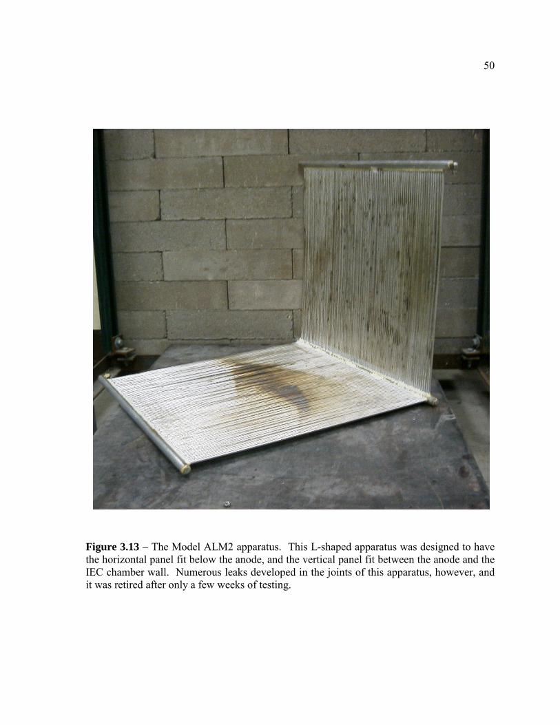
50
Figure 3.13 – The Model ALM2 apparatus. This L-shaped apparatus was designed to have the horizontal panel fit below the anode, and the vertical panel fit between the anode and the IEC chamber wall. Numerous leaks developed in the joints of this apparatus, however, and it was retired after only a few weeks of testing.
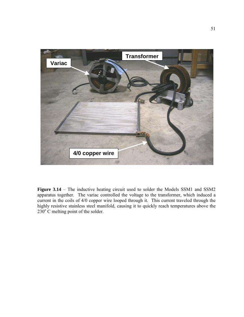
51
4/0 copper wire
TransformerVariac
Figure 3.14 – The inductive heating circuit used to solder the Models SSM1 and SSM2 apparatus together. The variac controlled the voltage to the transformer, which induced a current in the coils of 4/0 copper wire looped through it. This current traveled through the highly resistive stainless steel manifold, causing it to quickly reach temperatures above the 230o C melting point of the solder.
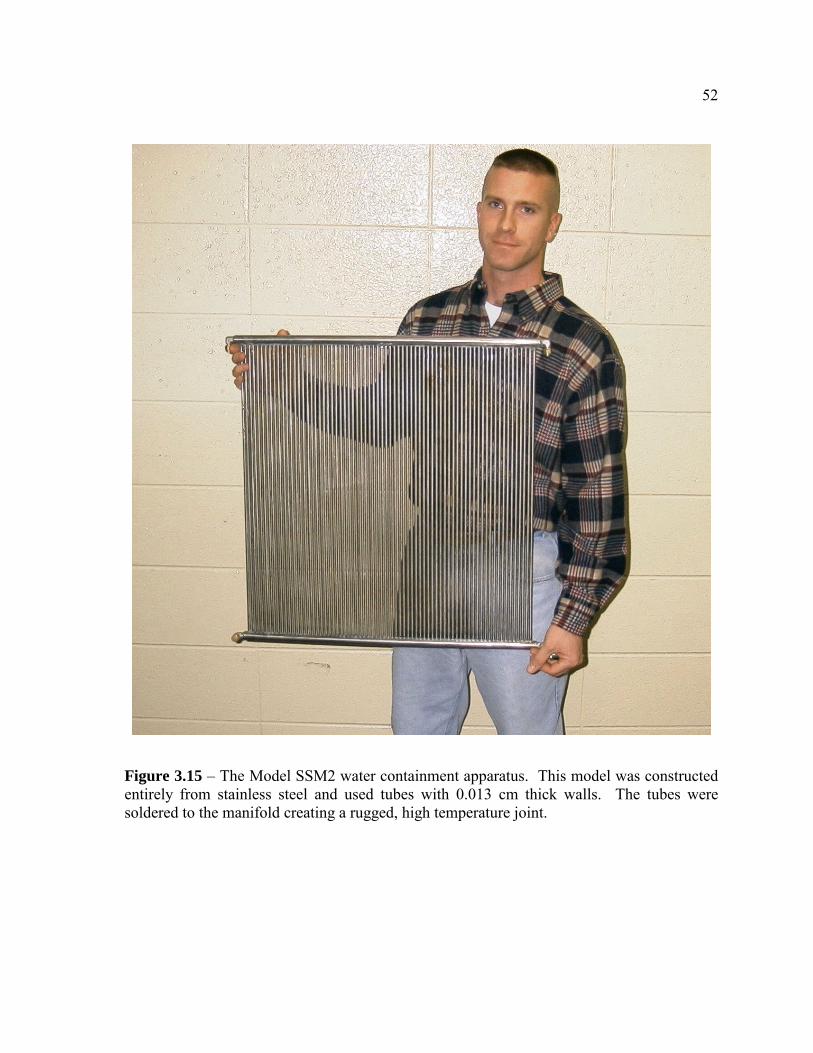
52
Figure 3.15 – The Model SSM2 water containment apparatus. This model was constructed entirely from stainless steel and used tubes with 0.013 cm thick walls. The tubes were soldered to the manifold creating a rugged, high temperature joint.
53
Chapter 4 Theory of 13N Activation in UW IEC
Section 4.1 Theory of Radioisotope Production in a Pure Thick Target
This chapter develops the equations required to predict the quantity of radioisotopes
produced by a proton flux impinging upon a target. The derived expressions are then
compared to experimental values and used to estimate the quantity of 13N that could be
produced by the IEC for specific operating conditions. This development follows that
described by Dr. Hesham Khater in his doctoral thesis completed in 1990 [28]. Several
assumptions are made in developing this theory.
1) The radioisotope is only produced by nuclear interactions between protons and
the parent atoms.
2) The number of parent atoms is not affected by the production of the daughter
radioisotope (i.e., there is no burn up of the parent atoms).
3) The only removal mechanism for the radioactive daughter atoms is radioactive
decay (i.e., the radioactive daughter atoms are not transmutated by the protons)
For a thin target of thickness �x containing only parent atoms, the creation of
radioisotopes and their decay during production is described by a simple balance equation.
For this equation, a thin target is defined to be a target of such thickness that the energy a
proton would lose in passing through it is negligible:
σ x λdN ndt
�� � � N (4.1)
54
where
N = the number of radioactive daughter atoms produced
� (cm2) = the parent atom’s nuclear cross section for proton absorption
n (atoms/g) = the number of parent atoms per gram of target material; the unit of
atoms per gram, rather than atoms per cubic centimeter, is used because the
density (atoms/cm3) of materials has the drawback of being temperature
dependent.
� (protons/s) = the number of protons impinging upon the target per second
�x (g/cm2) = the thickness of the thin target
� (s-1) = the decay constant of the radioisotope produced (= 1/ 2
ln 2T
)
Integrating the above equation yields the following expression, which predicts the number of
radioactive atoms produced during an irradiation of time t in seconds:
1σ x λ
teN n�
��� ��
� � ��
� (4.2)
Since the activity of N radioactive atoms is defined as the product of N and �, the
activity of the thin target can the be rewritten as:
(4.3) λ σ x (1 ) (dps)tA N n e �� �
� � � �
The activity of a thick target, defined as a target in which the proton expends all of
its kinetic energy, can be found by integrating equation (4.3) over the range Rp (g/cm2) of the
proton. This leads to the following relation:
(4.4) λ
0(1 ) σ( ) ( ) (dps)pRtA e n x x dx��
� � �

55
where the zero in the integral represents the target’s surface.
As described in Chapter 3, this experiment uses 14.7 MeV protons created from D-
3He fusion reactions to irradiate a target. It is assumed these protons are emitted from a
point source located in the center of the cathode. Since nuclear cross sections for protons
are generally very small at energies below 40 MeV, it’s assumed that the number of protons
lost due to nuclear reactions within the target is negligibly small [29]. In the case of a point
source of protons, it’s also assumed that the source is far enough away from the target that
the 1/r2 decrease in the flux is negligible over the range of the proton. Hence, the proton
flux is constant for all depths within the target and is redefined as o. It can then be moved
outside the integral, and equation (4.4) can be rewritten as:
(4.5) λ
0(1 ) σ( ) (dps)pRt
oA e n x dx��
� � �
Since cross sections are published as functions of energy rather than depth, the
integral in equation (4.5) is converted to an energy-dependent function by dividing the cross
section by the stopping power of the parent atom, S(E), in units of MeV�g/cm2. The
resulting integral is then evaluated over the energy range of the incident protons, where Ep
(MeV) is the proton’s initial energy:
λ
0
σ( )(1 ) (dps)( )
pEto
EA e n dES E
��
� � � (4.6)
Since accelerators and cyclotrons produce essentially all of the short-lived medical
radioisotopes, it’s convenient to further modify equation (4.6) such that its units reflect those
common to the commercial radioisotope production community. The proton beam in
accelerators and cyclotrons is measured as a current I (�A). If the proton flux in the IEC is
56
measured as a current, and recognizing that 1 �A of proton current is equivalent to 6.25 x
1012 p/s, equation (4.6) becomes
12 λ
0
σ( )6.25 x 10 (1 ) ( ) (dps)( )
pEt EA e I A n dES E
��
� � � (4.7)
The medical isotope community still often measures the activity of radionuclides in
units of Ci or some fraction thereof, rather than the SI standard of Bq. Hence, the units of
equation (4.7) are converted from Bq to mCi:
5 λ
0
σ( )1.689 x 10 (1 ) ( ) (mCi)( )
pEt EA e I A n dES E
��
� � � (4.8)
When evaluated, the integral in equation (4.8) is a constant value for a
monoenergetic proton flux. Hence, the only variables affecting the activity of a target
irradiated with protons of initial energy Ep is the irradiation time t and the proton current I.
If the expressions containing these two variables are removed from the relation, the
remaining value represents the maximum achievable activity for an infinite irradiation time
per unit of incident proton current of energy Ep. This value is known as the saturated yield,
Y, of the target and is given by:
�5
0
σ( )1.689 x 10 mCi µ( )
pE EY n dES E
� � �A (4.9)
Therefore, by substituting the above expression for the yield into equation (4.8), the target
activity can be cleanly written as:
(4.10) (1 ) (mCi)tA Y I e ��� �

57
Section 4.2 Modification of Production Yield for Homogeneous Mixtures
As previously stated, the above derivations apply to a target containing only parent
atoms of interest. In this experiment, however, the target oxygen atoms are contained within
water. Consequently, equation (4.10) must be modified to reflect the concentration of the
oxygen atoms within the water target and the difference in stopping power between oxygen
atoms and water molecules. This is accomplished using the equation [29]:
(4.11) η w O wY Y F�
where
Yw = saturated yield of water target
YO = saturated yield of oxygen target
w = weight concentration of the oxygen atoms in water
F = factor that accounts for the difference in stopping power between oxygen atoms
and water molecules
For water, w = 16/18 = 0.889.
The factor F can be found in at least three ways [30-33]. For this experiment, it is
calculated using the expression:
w
O
RFR
� (4.12)
where
Rw (g/cm2)= range of a proton of energy Ep in water = 0.2444 g/cm2 [27]
RO (g/cm2) = range of a proton of energy Ep in oxygen = 0.2844 g/cm2 [27]
Using the values of Rw and RO listed above, F is calculated to be 0.859.

58
From these values of w and F, the saturated yield of a water target is calculated to
be:
(4.13) (0.889) (0.859) = 0.764 (mCi/µA)w O OY Y Y�
The activity of a water target can then be found from this saturated yield as:
(4.14) 0.764 (1 ) (mCi)tOA Y I e ��
� �
Section 4.3 Calculation of 13N Yield in Water Target
In order to apply equation (4.14), the yield YO must be determined. Solving equation
(4.9) for protons of a specific initial energy accomplishes this. As mentioned in Chapter 3,
the energy of the 14.7 MeV protons from D-3He reactions is reduced by approximately 2.2
MeV as they pass through the 0.013 cm wall of the stainless steel tubing en-route to the
water inside. Hence, their initial energy upon entering the water is considered to be 12.5
MeV. For this initial proton energy, the cross sections [1] and stopping powers [27] are
obtained at 0.1 MeV intervals over the energy range in which the cross section has a non-
zero value (5.8 MeV – 12.5 MeV). These values are listed in table 4.1 at the end of this
chapter. The value of the integral in equation (4.9) is then approximated using the Midpoint
Rule [34]:
1
( ) ( ) nb
iaf E dE f E E� �� � (4.15)
where
�E = b an�
Ei = ½ (Ei-1 + Ei) = midpoint of [Ei-1, Ei]
For this calculation,
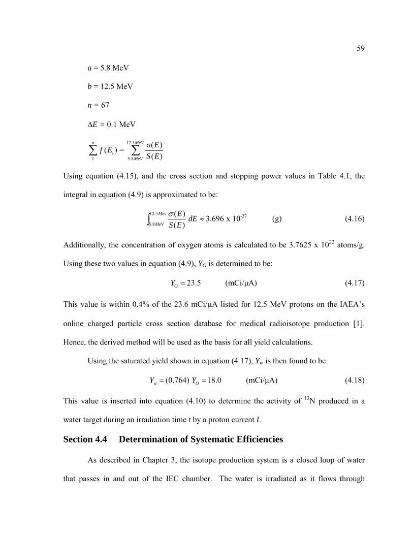
59
a = 5.8 MeV
b = 12.5 MeV
n = 67
�E = 0.1 MeV
12.5
1 5.8
σ( )( ) = ( )
n MeV
iMeV
Ef ES E� �
Using equation (4.15), and the cross section and stopping power values in Table 4.1, the
integral in equation (4.9) is approximated to be:
12.5 -27
5.8
( ) 3.696 x 10 (g)( )
Mev
MeV
E dES E�
�� (4.16)
Additionally, the concentration of oxygen atoms is calculated to be 3.7625 x 10²² atoms/g.
Using these two values in equation (4.9), YO is determined to be:
(4.17) 23.5 (mCi/µA)OY �
This value is within 0.4% of the 23.6 mCi/�A listed for 12.5 MeV protons on the IAEA’s
online charged particle cross section database for medical radioisotope production [1].
Hence, the derived method will be used as the basis for all yield calculations.
Using the saturated yield shown in equation (4.17), Yw is then found to be:
(4.18) (0.764) 18.0 (mCi/µA)w OY Y� �
This value is inserted into equation (4.10) to determine the activity of 13N produced in a
water target during an irradiation time t by a proton current I.
Section 4.4 Determination of Systematic Efficiencies
As described in Chapter 3, the isotope production system is a closed loop of water
that passes in and out of the IEC chamber. The water is irradiated as it flows through

60
numerous round, stainless steel tubes vertically aligned within the chamber. When
irradiation is complete, the water is removed from this system and passed through an ion
exchange resin that traps the 13NH3+ ions.
The physical design of the water containment apparatus degrades the energy of the
protons entering the water target. Moreover, the IEC fusion chamber, the mechanical
methods used to extract the water and the chemical process used to trap the 13NH3+ ions have
an inherent efficiency. Consequently, some 13N atoms will be lost during the production,
removal and capture processes. The energy of the protons entering the water target, as well
as all possible process efficiencies, must be known in order to accurately compare the
measured activity to the predicted activity. Eight isotope production characteristics that
either degrade the protons’ energy or affect the 13N collection efficiency have been
identified and are listed below. The calculated or estimated efficiency for each factor is
listed in parenthesis after it is identified.
1) Solid angle of target (0.10): This efficiency represents the fraction of D-3He
protons created that actually strike the Model SSM2 target. The ratio of the number of
protons impinging upon the water target to the number of D-3He fusion protons created is
determined by the target size. If the target intercepted every proton created within the IEC
chamber, this target would be 100% efficient at intercepting the protons. The model SSM2
target contained 70 tubes; the width of this target, measured from the outer edges of the end
tubes, is 60 cm. The height of the tubes is also 60 cm. Assuming that this area represents a
solid target surface (i.e. no space between the tubes), then the target would have a projected
surface area of 3600 cm2. The model SSM2 target is located approximately 33 cm from the
center of the chamber, and its geometric center is in the same vertical and horizontal plane

61
as the approximated point source of protons. At that location, a solid target of 3600cm2
represents a solid angle of 0.138 (the solid target would intercept 13.8% of the protons
produced at a point source located in the center of the chamber). But the SSM2 target is not
solid – there are small spaces between each pair of vertical tubes. Each tube has a projected
width of 0.64 cm, and a projected height of 60 cm, resulting in a combined cross sectional
surface area of only 2667 cm2 for all 70 tubes. In other words, the actual SSM2 target
surface area is only 74% of the surface area of the solid square target previously assumed.
This leads to an actual solid angle of 0.10. Thus, only about 10% of the protons produced
from a point source in the center of the cathode would actually impinge upon the tubes of
the SSM2 target.
2) Shadow effect of cathode wires (0.5): Current theories regarding D-3He fusion
within the IEC estimate that most D-3He fusion reactions occur within the wires of the
cathode [25]. These embedded reactions occur at sites where 3He ions have been implanted.
Assuming all reactions are embedded, half of the D-3He protons created will travel into the
cathode wire due to their isotropic distribution. These grid wires are much thicker than the
range of a 14.7 MeV proton. Hence, half of the protons produced as a result of embedded
reactions are lost within the cathode.
3) Proton energy loss due to embedded reactions (0.998): This is an extension of the
shadow effect of the cathode grid wires discussed above. The depth of the embedded
reactions is thought to be approximately one micron deep. Depending upon the direction
they are ejected, the protons exiting the cathode wires will travel through varying
thicknesses of material. The resulting proton current will no longer be monoenergetic; the
protons will have a spectrum of energies below 14.7 MeV, which will have the net affect of

62
decreasing the 13N yield. The stopping power of tungsten is 271 MeV/cm [27]. Assuming
pure tungsten cathode wires, an average embedded reaction depth of one micron, and that
the average proton is ejected at an angle of 45o with respect to the normal direction, the
average thickness of material the proton will pass through is about 1.4 microns. A 14.7
MeV proton traveling through 1.4 microns of tungsten will only lose approximately 0.03
MeV, or 0.2 % of its energy. Assuming the yield is affected by this same amount, this factor
is deemed to be 0.998.
4) Cathode transparency (0.96): Based on the projected area of its wires, the
cathode transparency has been calculated to be 0.92 for ions accelerated towards it. During
isotope production, this factor represents the fraction of protons that are not intercepted by
the cathode wires as the protons travel out of the region bounded by the cathode (from
embedded reactions). Only half of the protons directed towards the target will have to exit
the region bounded by the cathode, and thus be attenuated by the cathode wires; those
protons created on the cathode wire surfaces facing outward are already outside the cathode.
Therefore, this efficiency is calculated as (p/2 + 0.92p/2) = 0.96p, where p is the fraction of
protons exiting the region bounded by the cathode.
5) Anode transparency (0.95): Like the cathode, the anode will also intercept a
small percentage of the protons that are traveling towards the water target. The fraction of
protons that are not intercepted by the anode has been calculated to be 0.95 based on the
projected area the wires.
6) Tube geometry (0.60): Because of the round geometry of the tubes in the model
SSM2 target, the wall thickness that a proton would see, if it were incident perpendicularly
to the projected area of the tube, changes as one moves from the center to the lateral edges

63
of the tube. This is illustrated in Figure 4.1 and Figure 4.2. If a proton strikes at a location
75o (5�/12 rad) or greater from the center of the tube with respect to the normal direction,
the wall thickness is so great that the proton’s energy is reduced below the nuclear cross
section threshold (5.8 MeV). Those protons will not create 13N even if they pass through to
the water. Moreover, a proton also experiences different wall thickness depending upon
what angle it strikes the tube with respect to the horizontal plane of the chamber (see Figure
4.3). A proton incident on the vertical center of the tube, which is in the same horizontal
plane as the theoretical point source of protons, would impinge at an angle of zero relative to
the horizontal plane. A proton impinging at either the top or bottom of a tube would be
incident at an angle of approximately 42.3o (0.738 rad) to the horizontal plane for the SSM2
target located 33 cm from the point source with tubes 60 cm tall. The average wall
thickness a proton experiences can be approximated by integrating in both planes as shown
below:
5 0.73812
0 0
12 1 0.0127 cm = 0.0218 cm5 0.738 cos cos
d dT�
� �
� � �� � � (4.19)
In stainless steel, a 14.7 MeV proton experiences a stopping power of 172.2 MeV/cm [27].
Thus, the average wall thickness of 0.0218 cm results in protons with an average energy of
approximately 10.9 MeV – much less than the 12.5 MeV previously assumed. The yield of
a 10.9 MeV proton is calculated using Table 4.1 in the same manner as described in Section
4.3 for 12.5 MeV protons. The resulting yield is 11.2 mCi/�A, which is only 0.62 of the
yield for 12.5 MeV protons. Recall, however, that only those protons striking the tube from
0 to 5�/12 rad have been accounted for. The projected width of the tubes from -5�/12 rad to
64
+5�/12 rad represents 0.966 of the total projected tube width 5πsin12
πsin2
� �� �
� �� �
� . These two
fractions are multiplied to yield the total efficiency due to tube geometry of 0.60.
�
7) Water recovery (0.91): The entire closed loop of the isotope production system
holds approximately 1650 mL of water. When the system is pressurized with helium, only
1500 mL of water is expelled from the system and into the ion exchange resin. Much of the
water remaining in the system (about 100 mL) is contained in the water expansion reservoir
that is in-line with the system but not pressurized when the system is emptied. The other 50
mL of water is assumed to be trapped in the pump and SSM2 target. The 1500 mL of
expelled water represents a 0.91 water recovery efficiency.
8) Resin capture (0.95): The true efficiency of the resin’s ability to capture the 13N
atoms can only be estimated. In order to measure the efficiency, one could measure the
activity of the 13N that passed through the resin and compare that to the activity of the 13N
captured within the resin. The minute quantity of 13N produced in this experiment made it
impossible to accurately measure any 13N activity that may have remained in the
approximately 1.5 liters of water that passed through the resin. The 13N concentration in this
water is simply too low to measure with the equipment available. Moreover, it’s likely that
a small fraction of 13N atoms form 13NH2�, 13NO3
�, and 13NO2� ions, which will not be
trapped by the DOWEX cation exchange resin. To ensure the resin efficiency was
maximized, the amount of ion exchange resin used was larger than that believed necessary.
Additionally, the water contained 10 millimolar ethyl alcohol to promote the production of
13NH3+ ions. Therefore, the resin efficiency is estimated to be 95%.
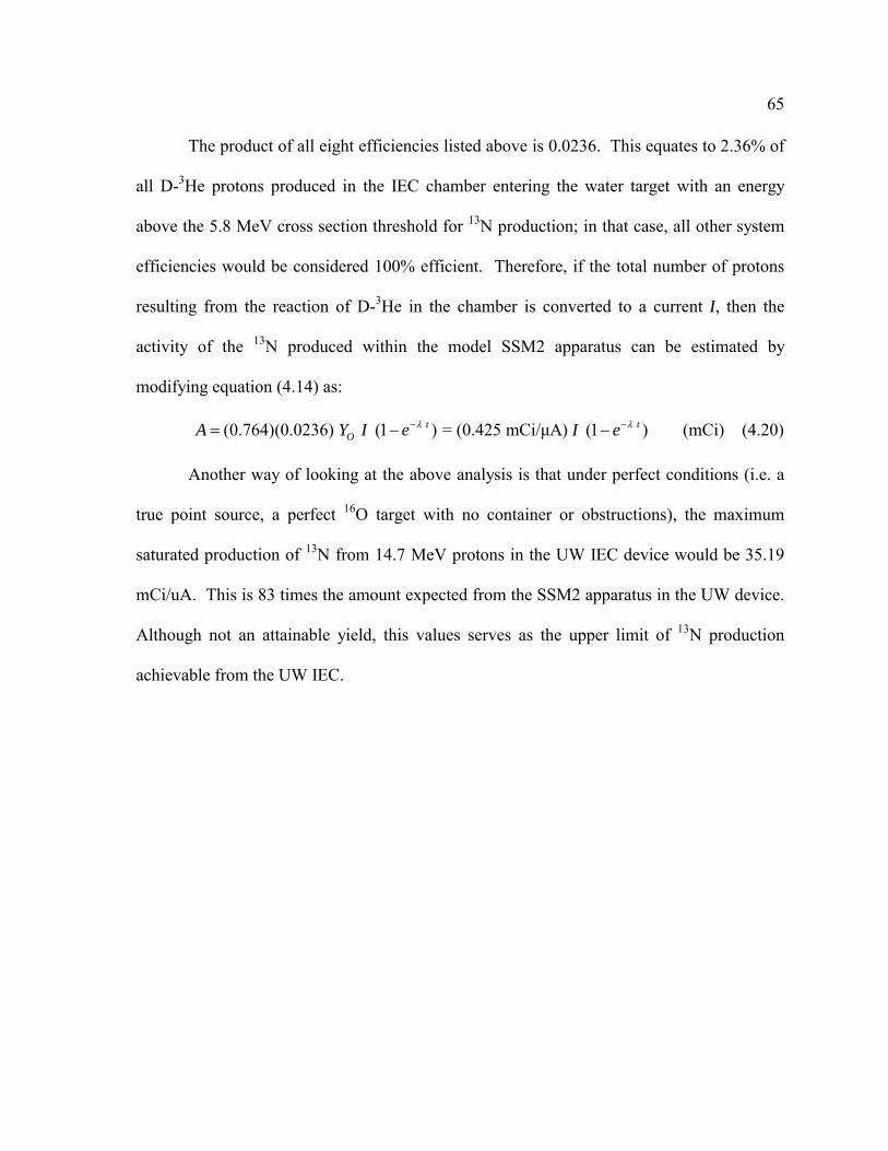
65
The product of all eight efficiencies listed above is 0.0236. This equates to 2.36% of
all D-3He protons produced in the IEC chamber entering the water target with an energy
above the 5.8 MeV cross section threshold for 13N production; in that case, all other system
efficiencies would be considered 100% efficient. Therefore, if the total number of protons
resulting from the reaction of D-3He in the chamber is converted to a current I, then the
activity of the 13N produced within the model SSM2 apparatus can be estimated by
modifying equation (4.14) as:
(4.20) (0.764)(0.0236) (1 ) = (0.425 mCi/µA) (1 ) (mCi)t tOA Y I e I e� �� �
� � �
Another way of looking at the above analysis is that under perfect conditions (i.e. a
true point source, a perfect 16O target with no container or obstructions), the maximum
saturated production of 13N from 14.7 MeV protons in the UW IEC device would be 35.19
mCi/uA. This is 83 times the amount expected from the SSM2 apparatus in the UW device.
Although not an attainable yield, this values serves as the upper limit of 13N production
achievable from the UW IEC.

66
Table 4.1 - This table is used to solve the integral in equation (4.9) using the midpoint rule. Note that the column on the far right provides the solution to the interval forenergy E + 0.5 MeV. The pertinent values in this column are in bold.
E (Mev) ��(mb)
[1] � (cm2)
[27] S (MeV-cm2/g)
��/ S (g/MeV)�
�/S at energy E + 0.05 MeV�
����S from 5.8 MeV to energy E + 0.5 MeV�
5.8 0.0 5.74E-30 60.31 9.52E-32 2.459E-30 2.459E-30 5.9 0.3 2.87E-28 59.52 4.82E-30 7.688E-30 1.015E-29 6.0 0.6 6.20E-28 58.75 1.06E-29 1.347E-29 2.361E-29 6.1 1.0 9.50E-28 58.00 1.64E-29 1.788E-29 4.149E-29 6.2 1.1 1.11E-27 57.28 1.94E-29 1.772E-29 5.921E-29 6.3 0.9 9.09E-28 56.57 1.61E-29 1.197E-29 7.119E-29 6.4 0.4 4.40E-28 55.88 7.87E-30 4.652E-30 7.584E-29 6.5 0.1 7.90E-29 55.21 1.43E-30 8.557E-31 7.669E-29 6.6 0.0 1.53E-29 54.56 2.80E-31 2.282E-30 7.898E-29 6.7 0.2 2.31E-28 53.92 4.28E-30 8.493E-30 8.747E-29 6.8 0.7 6.77E-28 53.30 1.27E-29 1.906E-29 1.065E-28 6.9 1.3 1.34E-27 52.70 2.54E-29 3.411E-29 1.406E-28 7.0 2.2 2.23E-27 52.11 4.28E-29 5.439E-29 1.950E-28 7.1 3.4 3.40E-27 51.53 6.60E-29 8.106E-29 2.761E-28 7.2 4.9 4.90E-27 50.97 9.61E-29 1.153E-28 3.914E-28 7.3 6.8 6.78E-27 50.42 1.34E-28 1.582E-28 5.496E-28 7.4 9.1 9.08E-27 49.89 1.82E-28 2.105E-28 7.602E-28 7.5 11.8 1.18E-26 49.36 2.39E-28 2.690E-28 1.029E-27 7.6 14.6 1.46E-26 48.85 2.99E-28 3.273E-28 1.356E-27 7.7 17.2 1.72E-26 48.36 3.56E-28 3.763E-28 1.733E-27 7.8 19.0 1.90E-26 47.87 3.97E-28 2.099E-27 3.832E-27 7.9 180.1 1.80E-25 47.39 3.80E-27 2.447E-27 6.279E-27 8.0 51.3 5.13E-26 46.93 1.09E-27 9.812E-28 7.260E-27 8.1 40.4 4.04E-26 46.47 8.69E-28 8.443E-28 8.104E-27 8.2 37.7 3.77E-26 46.02 8.19E-28 8.132E-28 8.918E-27 8.3 36.8 3.68E-26 45.59 8.07E-28 8.155E-28 9.733E-27 8.4 37.2 3.72E-26 45.16 8.24E-28 8.515E-28 1.058E-26 8.5 39.3 3.93E-26 44.74 8.79E-28 9.055E-28 1.149E-26 8.6 41.3 4.13E-26 44.33 9.32E-28 7.911E-28 1.228E-26 8.7 28.6 2.86E-26 43.93 6.51E-28 4.592E-28 1.274E-26 8.8 11.7 1.17E-26 43.53 2.68E-28 3.344E-28 1.307E-26 8.9 17.3 1.73E-26 43.14 4.01E-28 2.625E-28 1.334E-26 9.0 5.3 5.30E-27 42.76 1.24E-28 1.231E-28 1.346E-26
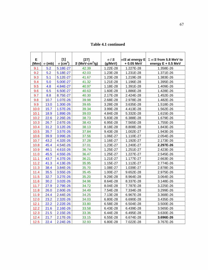
67
Table 4.1 continued
E (Mev) ��(mb)�
[1] � (cm2)
[27] S (MeV-cm2/g)
��/ S (g/MeV)�
�/S at energy E + 0.05 MeV�
����S from 5.8 MeV to energy E + 0.5 MeV�
9.1 5.2 5.18E-27 42.39 1.22E-28 1.227E-28 1.358E-26 9.2 5.2 5.18E-27 42.03 1.23E-28 1.231E-28 1.371E-26 9.3 5.1 5.12E-27 41.67 1.23E-28 1.219E-28 1.383E-26 9.4 5.0 5.00E-27 41.32 1.21E-28 1.196E-28 1.395E-26 9.5 4.8 4.84E-27 40.97 1.18E-28 1.391E-28 1.409E-26 9.6 6.5 6.50E-27 40.63 1.60E-28 1.886E-28 1.428E-26 9.7 8.8 8.75E-27 40.30 2.17E-28 2.424E-28 1.452E-26 9.8 10.7 1.07E-26 39.98 2.68E-28 2.978E-28 1.482E-26 9.9 13.0 1.30E-26 39.65 3.28E-28 3.635E-28 1.518E-26 10.0 15.7 1.57E-26 39.34 3.99E-28 4.413E-28 1.562E-26 10.1 18.9 1.89E-26 39.03 4.84E-28 5.332E-28 1.615E-26 10.2 22.6 2.26E-26 38.73 5.83E-28 6.388E-28 1.679E-26 10.3 26.7 2.67E-26 38.43 6.95E-28 7.565E-28 1.755E-26 10.4 31.2 3.12E-26 38.13 8.18E-28 8.808E-28 1.843E-26 10.5 35.7 3.57E-26 37.84 9.43E-28 1.002E-27 1.943E-26 10.6 39.9 3.99E-26 37.56 1.06E-27 1.110E-27 2.054E-26 10.7 43.2 4.32E-26 37.28 1.16E-27 1.192E-27 2.173E-26 10.8 45.4 4.54E-26 37.01 1.23E-27 1.240E-27 2.297E-26 10.9 46.1 4.61E-26 36.74 1.25E-27 1.251E-27 2.423E-26 11.0 45.5 4.55E-26 36.47 1.25E-27 1.227E-27 2.545E-26 11.1 43.7 4.37E-26 36.21 1.21E-27 1.177E-27 2.663E-26 11.2 41.3 4.13E-26 35.95 1.15E-27 1.112E-27 2.774E-26 11.3 38.4 3.84E-26 35.70 1.08E-27 1.039E-27 2.878E-26 11.4 35.5 3.55E-26 35.45 1.00E-27 9.652E-28 2.975E-26 11.5 32.7 3.27E-26 35.20 9.29E-28 8.964E-28 3.064E-26 11.6 30.2 3.02E-26 34.96 8.64E-28 8.337E-28 3.148E-26 11.7 27.9 2.79E-26 34.72 8.04E-28 7.787E-28 3.225E-26 11.8 26.0 2.60E-26 34.49 7.54E-28 7.334E-28 3.299E-26 11.9 24.4 2.44E-26 34.25 7.13E-28 6.967E-28 3.368E-26 12.0 23.2 2.32E-26 34.03 6.80E-28 6.690E-28 3.435E-26 12.1 22.2 2.22E-26 33.80 6.58E-28 6.504E-28 3.500E-26 12.2 21.6 2.16E-26 33.58 6.43E-28 6.439E-28 3.565E-26 12.3 21.5 2.15E-26 33.36 6.44E-28 6.495E-28 3.630E-26 12.4 21.7 2.17E-26 33.15 6.55E-28 6.674E-28 3.696E-26 12.5 22.4 2.24E-26 32.93 6.80E-28 7.022E-28 3.767E-26

68
Table 4.1 continued
E (Mev) ��(mb)�
[1] � (cm2)
[27] S (MeV-cm2/g)
��/ S (g/MeV)�
�/S at energy E + 0.05 MeV�
����S from 5.8 MeV to energy E + 0.5 MeV�
12.6 23.7 2.37E-26 32.73 7.24E-28 7.480E-28 3.842E-26 12.7 25.1 2.51E-26 32.52 7.72E-28 7.881E-28 3.920E-26 12.8 26.0 2.60E-26 32.32 8.04E-28 7.914E-28 3.999E-26 12.9 25.0 2.50E-26 32.12 7.78E-28 7.338E-28 4.073E-26 13.0 22.0 2.20E-26 31.92 6.89E-28 6.394E-28 4.137E-26 13.1 18.7 1.87E-26 31.72 5.90E-28 5.548E-28 4.192E-26 13.2 16.4 1.64E-26 31.53 5.20E-28 5.042E-28 4.243E-26 13.3 15.3 1.53E-26 31.34 4.88E-28 4.865E-28 4.291E-26 13.4 15.1 1.51E-26 31.15 4.85E-28 4.958E-28 4.341E-26 13.5 15.7 1.57E-26 30.97 5.07E-28 5.295E-28 4.394E-26 13.6 17.0 1.70E-26 30.78 5.52E-28 5.865E-28 4.453E-26 13.7 19.0 1.90E-26 30.60 6.21E-28 6.670E-28 4.519E-26 13.8 21.7 2.17E-26 30.43 7.13E-28 7.747E-28 4.597E-26 13.9 25.3 2.53E-26 30.25 8.36E-28 9.069E-28 4.687E-26 14.0 29.4 2.94E-26 30.08 9.77E-28 1.052E-27 4.793E-26 14.1 33.7 3.37E-26 29.91 1.13E-27 1.185E-27 4.911E-26 14.2 37.0 3.70E-26 29.74 1.24E-27 1.266E-27 5.038E-26 14.3 38.1 3.81E-26 29.57 1.29E-27 1.266E-27 5.164E-26 14.4 36.6 3.66E-26 29.41 1.24E-27 1.195E-27 5.284E-26 14.5 33.5 3.35E-26 29.24 1.15E-27 1.088E-27 5.393E-26 14.6 30.0 3.00E-26 29.08 1.03E-27 9.866E-28 5.491E-26 14.7 27.2 2.72E-26 28.92 9.42E-28 4.708E-28 5.538E-26

69
5 rad12�
� �
B
A 2
1
Figure 4.1 – The thickness of the tube wall of the SSM2 target changes for a proton striking perpendicularly to the cross-sectional plane. Hence, a proton striking at point 2 must travel through more stainless steel than a proton striking at point 1.
2
1
Figure 4.2 – The width of the tube A represents the frontal projected width of a tube in which an incident proton is still capable of undergoing nuclear reactions once it reaches the water. The width B represents the total projected tube width. Width A is 96.6% of the entire tube width B.
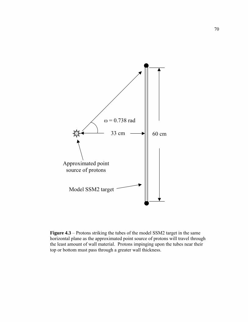
70
Model SSM2 target
Approximated point source of protons
��= 0.738 rad
60 cm33 cm
Figure 4.3 – Protons striking the tubes of the model SSM2 target in the same horizontal plane as the approximated point source of protons will travel through the least amount of wall material. Protons impinging upon the tubes near their top or bottom must pass through a greater wall thickness.
71
Chapter 5 Experimental Technique and Equipment
Section 5.1 Water Target and Ion Exchange Resin Preparation
The two most important items for this experiment are the water target and the ion
exchange resin. To optimize the performance of these two critical items, the same
preparation and experimental procedure was followed for every attempted production run.
As discussed in Chapter 3, the DOWEX 50WX8 (100-200) cation exchange resin will
capture a variety of cations. Moreover, the quantity of ions the resin can hold is limited.
Once all the ionic exchange sites are expended, no additional ions passing through the resin
will be captured. Consequently, the radioisotope production system needed to be as free of
contaminant ions as possible to ensure every 13N atom was captured. During the many
conditioning runs leading up to a production run, reverse osmosis water was used in the
closed-loop production system to keep it as clean as possible. This water was also changed
every day. Prior to a production run, the closed-loop water circuit was rinsed three times
with 18 M�-cm water. For the first rinse, the system was briefly flushed with 18 M�-cm
water. The system was then filled with pure 18 M�-cm water, which was circulated for
approximately 1 hour. It was then flushed a second time with 18 M�-cm water and then
again filled with pure water, which was circulated for approximately 30 minutes. The
system was flushed a third time and filled with 18 M�-cm water, which was circulated for
15 minutes. Finally, the system was filled with 18 M�-cm water containing 10 millimolar
ethyl alcohol to promote the formation of 13NH3+ ions.
A special plastic container was used to transport the 18 M�-cm water. Before it was
filled, it was first rinsed with reverse osmosis water, then with 18 M�-cm water. It was
72
then filled with argon gas to minimize the formation of carbonic acid caused by the
interaction of the pure water with the carbon dioxide in the atmosphere. The 18 M�-cm
water was then poured into the container.
The ion exchange resin also had to be prepared prior to each production run. The
first step was to place approximately 25 grams of DOWEX 50WX8 (100-200) cation
exchange resin into a clean glass beaker. This quantity of resin was chosen because it filled
the column to a height of nearly three inches, which is the width of the NaI crystal used to
count the activity of 13N trapped in the resin. In other words, the column contained the
maximum amount of resin that would fit within the boundaries of the detector face. Next,
100 mL of 0.1 molar NaOH was mixed with the resin for several minutes to recharge the
ionic sites with the Na+ ions in this solution. During the production run, these Na+ ions
would exchange with 13NH3+ ions in the water, capturing the ammonia in the resin in the
same manner as a water softener removes minerals from a household water supply.
The resin column, which was just a 60 cc plastic syringe, was thoroughly rinsed with
18 M�-cm water. A bundle of glass wool was then placed at the bottom of the syringe. The
glass wool served as a filter by allowing the water to easily pass through but retaining the
resin in the syringe. The NaOH and resin solution was then poured into the column
(syringe). To remove the traces of resin remaining in the beaker, it was rinsed several times
with small amounts of 18 M�-cm water, which was also poured into the syringe. As
necessary, the syringe plunger was used to force this solution through the resin and out of
the syringe. Additional 18 M�-cm water was then slowly poured into the syringe and
forced through the resin. This was done approximately 20 times to rinse the NaOH from the

73
resin. It was very important to ensure all NaOH was removed. If some NaOH remained
trapped in the resin, the Na+ ions could exchange with sites containing 13N atoms during a
production run. These 13N atoms might then be lost. After this rinsing cycle, the pH of the
water was measured to ensure that after passing through the resin it was 7. This indicated
that all of the NaOH had been removed.
After flushing the resin column thoroughly, it was connected to the isotope
extraction system with an airtight clamp. An exploded view of the resin column and
clamping mechanism is shown in figure 5.1. Figure 5.2 shows a picture of the column with
the ion exchange resin inside, and a picture of the column fully assembled is shown in figure
5.3. The airtight clamp enabled the column to be pressurized, forcing the water through the
resin without leaks. The wastewater passing through the column was collected in a plastic
container and stored in the control room for several hours after each run. This water was
measured for radioactivity after many production runs, but no activity was ever detected.
Even so, it was stored prior to disposal to ensure any 13N or other short-lived radioisotopes
decayed away.
The last step in preparing the radioisotope production system was connecting a
pressurizing helium line. This helium line was maintained at 50 psi and was separated from
the system by a valve. When the production run was terminated, the valve was opened,
pressurizing the system and quickly forcing the water through the ion exchange resin
column. This process took approximately two minutes to complete. The resin column was
then disconnected from the water circuit, placed in a plastic bag to prevent radioactive
contamination from any water spilled onto its surface, and rushed to the 3 x 3 NaI detector
in the UW nuclear reactor (UWNR) lab, usually arriving within three minutes of shut down.
74
Section 5.2 Production Run Procedure
Once the water and ion exchange column were prepared and the IEC was ready for
an isotope production run, the large fan mounted in the IEC operation room was turned on.
The aluminum IEC chamber relies on air-cooling to dissipate the many kilowatts of power
generated inside. For an isotope production run, the IEC was operated at the highest power
possible, so the additional cooling of the fan was required to keep the rubber seals of the
chamber from exceeding their temperature limits. A second portable fan was placed facing
the side of the IEC opposite the large mounted fan. These two fans kept the surface of the
IEC chamber below 70o C during all production runs.
To help keep the chamber cool as long as possible, the filaments were turned off
several hours before the production run. This enabled the chamber to cool and reach
equilibrium with the surrounding room temperature. Additionally, the voltage and current
were brought to production levels as quickly as possible when the production run began.
Rather than stepping the voltage up in 10 kV increments as was typically done during
conditioning runs, the voltage was steadily increased to 100 kV in approximately one
minute. It was then allowed to operate at this voltage for about one minute, and was then
brought to production levels (~ 140 kV) over the next minute.
The chamber pressure was initial set to approximately 1.4 mtorr during production
runs. Previous pressure scans with D-3He fuel suggested that the reaction rate was
optimized at a pressure near 1.4 mtorr. However, the chamber tended to operate more
smoothly at pressures near 1.8 mtorr. The pressure often increased during any high power
run due to increased outgassing of the chamber as it was heated. The chamber pressure was

75
allowed to reach 1.8 mtorr before the fuel inflow rates were manually reduced to maintain
the pressure below 1.8 mtorr.
The ratio of D to 3He inside the IEC was maintained at 1:1 according to
measurements by the residual gas analyzer (RGA). Equal peaks do not necessarily mean
that the amount of each gas, either by weight or by volume, is equal. The method by which
the RGA analyzes gases can indicate that the peaks are equal even though the amount of
each gas present is not. This is referred to as the cracking pattern of a gas, and the cracking
pattern of many gasses are available in the RGA technical literature. This literature does not
list the cracking pattern for isotopes such as D and 3He, however, so the exact ratio of these
two gases is not precisely known. It was noted in previous IEC experiments that the D-3He
reaction rate was optimized (as measured by the proton detector) when these peaks were
matched on the RGA.
After the production run is terminated, the water circuit of the isotope production
system is pressurized with helium to quickly force it through the ion exchange resin column.
This is done by opening and closing a series of valves as shown in figure 5.4. First, the
water pump is unplugged. The water is forced out of the system in the opposite direction it
was circulated, so the pump must be off to reverse this flow. Next, the two valves
controlling water into and out of the expansion reservoir are closed. Following this, a valve
is opened that enables water to flow into the resin column. Last, a valve is opened that
pressurizes the water circuit with 50 psi helium, forcing the water out of the system and
through the resin column. The water is collected in a container as it passes out of the
column as shown in figure 5.4. The resin column is then detached, the plunger is inserted
into the syringe to compress the resin in as small a volume as possible, and the syringe is

76
placed in a plastic bag. The plastic bag prevents water from leaking out of the syringe and
contaminating the surrounding environment, such as the detector face, with radioactivity.
The activity of the 13N contained in the ion exchange resin was counted using a
single 3 x 3 NaI detector. A thin sheet of plastic is permanently mounted on the face of the
detector to protect it. As shown in figure 5.5, the column was placed on this plastic sheet
with the downstream edge of the resin immediately above the edge of the detector. This was
done assuming that the upstream end would have a higher 13N activity. This end would then
be closer to the middle of the detector, resulting in a higher counting efficiency.
The electronics associated with the detector system are detailed in the schematic
diagram of figure 5.6. The 3 x 3 NaI detector, photomultiplier tube (PMT) and base are
housed in a large lead vault to shield it from background radiation. These components were
manufactured by Teledyne Isotopes. A Canberra Model 3102 high voltage power supply is
used to bias the detector to +600 volts. The detector output is connected directly to the input
of an ORTEC Model 440A selectable active filter amplifier. The amplifier course gain is set
to 32x, the fine gain set to 2.3, and the shaping time set to 1 �s. The amplifier output signal
is fed to a multi-channel analyzer (MCA) installed in a desktop computer.
A region of interest (ROI) was set in the energy spectrum of the MCA. This ROI
extended from 470 keV to 570 keV and was established at either end of a 511 keV
photopeak using a 22Na source. This ROI would be used as the standard energy range with
which to compare the future activity of 13NH3 samples produced in the IEC. The MCA
software provided the gross number (sample plus background) of counts within the ROI. By
subtracting the background activity from the gross activity of the column, one can calculate
the net activity of 13NH3 in the resin.
77
Using the technique described in Chapter 4, the anticipated activity of 13N produced
in the IEC was on the order of 37 Bq (1 nCi). For an activity this small, it was determined
that the sample should be counted in two-minute intervals to provide counting statistics with
95% certainty. Since radioactive decay detection follows a Poisson distribution, the error �
in counting a sample activity is the square root of the number of counts [7]. The desired
statistical certainty can then be used to determine the total number of counts required from:
1NN N
� � � (5.1)
where N is the total detected number of counts. Once the total number of counts required
for a desired level of accuracy is known, the count time (in seconds) is easily determined by
dividing N by the anticipated activity in Bq.
Many two-minute count sequences would be done in order to establish a decay curve
for the radionuclide. The MCA was programmed to count for two minutes; the program did
not automatically log (save) the count data and restart, however, so this was done manually.
In this manner, numerous counts are made. As the activity of the sample decayed, the count
time required to obtain 95% should be increased. The count time was not increased for
these counts, though, for two reasons. First, it was extremely convenient to have the MCA
automatically terminate the count time at some preset length. This count time could not be
programmed for sequencially increasing count times; it could only be set for a single,
constant count time. Resetting the count time for each count interval would consume some
time and also invite errors. Second, it was desired to keep the count time to as small a
fraction of the half-life as possible. In doing this, the activity could be approximated as a
constant during the count time. Hence, each count of the resin column was done over a two-
78
minute interval. As described in Chapter 6, however, the count time was eventually
extended to three-minute intervals when it was determined that the activity of 13N created
was much less than anticipated.
When the counting process for the resin column was completed, a 10-minute
background reading was done. This is accomplished by removing the resin column from the
lead vault and setting the MCA to automatically count for 10 minutes. After adjusting the
background counts measured in 10 minutes to a 2-minute background count, it is subtracted
from the gross activity of the resin column to determine the net activity of the 13N trapped in
the resin.
In order to determine the true activity of the 13N in the column, the detector’s
efficiency at detecting 511 keV photons had to be determined. This was accomplished by
using a calibrated 22Na radiation source. The 22Na emits a positron during 89.9% of its
decays. The positron eventually collides with an electron, emitting two 511 keV gamma
rays in the same manner as 13N. For the detector efficiency measurement, the 22Na source
was not placed on the center of the detector face. Rather, it was located slightly off-center.
This was done to mimic the conditions of counting the resin column. It’s believed that the
upstream end of the resin column contains the highest concentration of 13N activity. Since
this portion of the column is located off center of the detector face as shown in figure 5.5,
the 22Na source was placed in the same area relative to the detector face.
The activity of the calibrated source at the time of the efficiency test was calculated
to be 82.0 nCi. This value is multiplied by 0.899 to account for only those decays that emit
a positron, resulting in an activity of 73.7 nCi or 2,729 Bq. A 300 second count of this
source detected 140,717 counts in the photopeak. This equates to a detected activity of 469
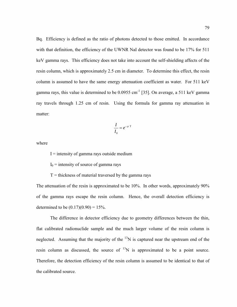
79
Bq. Efficiency is defined as the ratio of photons detected to those emitted. In accordance
with that definition, the efficiency of the UWNR NaI detector was found to be 17% for 511
keV gamma rays. This efficiency does not take into account the self-shielding affects of the
resin column, which is approximately 2.5 cm in diameter. To determine this effect, the resin
column is assumed to have the same energy attenuation coefficient as water. For 511 keV
gamma rays, this value is determined to be 0.0955 cm-1 [35]. On average, a 511 keV gamma
ray travels through 1.25 cm of resin. Using the formula for gamma ray attenuation in
matter:
T
0
I eI
���
where
I = intensity of gamma rays outside medium
I0 = intensity of source of gamma rays
T = thickness of material traversed by the gamma rays
The attenuation of the resin is approximated to be 10%. In other words, approximately 90%
of the gamma rays escape the resin column. Hence, the overall detection efficiency is
determined to be (0.17)(0.90) = 15%.
The difference in detector efficiency due to geometry differences between the thin,
flat calibrated radionuclide sample and the much larger volume of the resin column is
neglected. Assuming that the majority of the 13N is captured near the upstream end of the
resin column as discussed, the source of 13N is approximated to be a point source.
Therefore, the detection efficiency of the resin column is assumed to be identical to that of
the calibrated source.

80
Clamp
O-ring seal Spacer
Support
Column
Cap
Swageloc™ Fitting
Figure 5.1 – Exploded view of ion exchange column. The column is a 60 cc syringe plastic syringe. The syringe was placed in the support, which was mounted to the frame of the IEC chamber. The o-ring seals were used to create the airtight seal between the support and the cap. The clamp holds the entire assembly together. Water enters the column through the Swageloc™ fitting on the top of the cap.
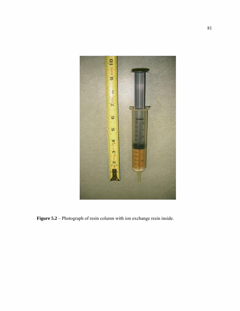
81
Figure 5.2 – Photograph of resin column with ion exchange resin inside.

82
Figure 5.3 – Ion exchange column mounted just below the IEC chamber. The water flows into the column through the plastic tubing at the top of the picture. After the water flows through the resin, it is collected in a waste container.
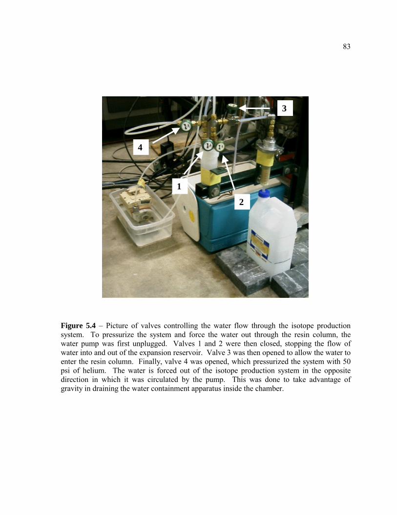
83
3
2
1
4
1
Figure 5.4 – Picture of valves controlling the water flow through the isotope production system. To pressurize the system and force the water out through the resin column, the water pump was first unplugged. Valves 1 and 2 were then closed, stopping the flow of water into and out of the expansion reservoir. Valve 3 was then opened to allow the water to enter the resin column. Finally, valve 4 was opened, which pressurized the system with 50 psi of helium. The water is forced out of the isotope production system in the opposite direction in which it was circulated by the pump. This was done to take advantage of gravity in draining the water containment apparatus inside the chamber.
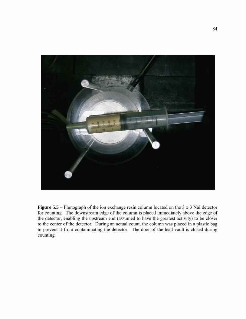
84
Figure 5.5 – Photograph of the ion exchange resin column located on the 3 x 3 NaI detector for counting. The downstream edge of the column is placed immediately above the edge of the detector, enabling the upstream end (assumed to have the greatest activity) to be closer to the center of the detector. During an actual count, the column was placed in a plastic bag to prevent it from contaminating the detector. The door of the lead vault is closed during counting.
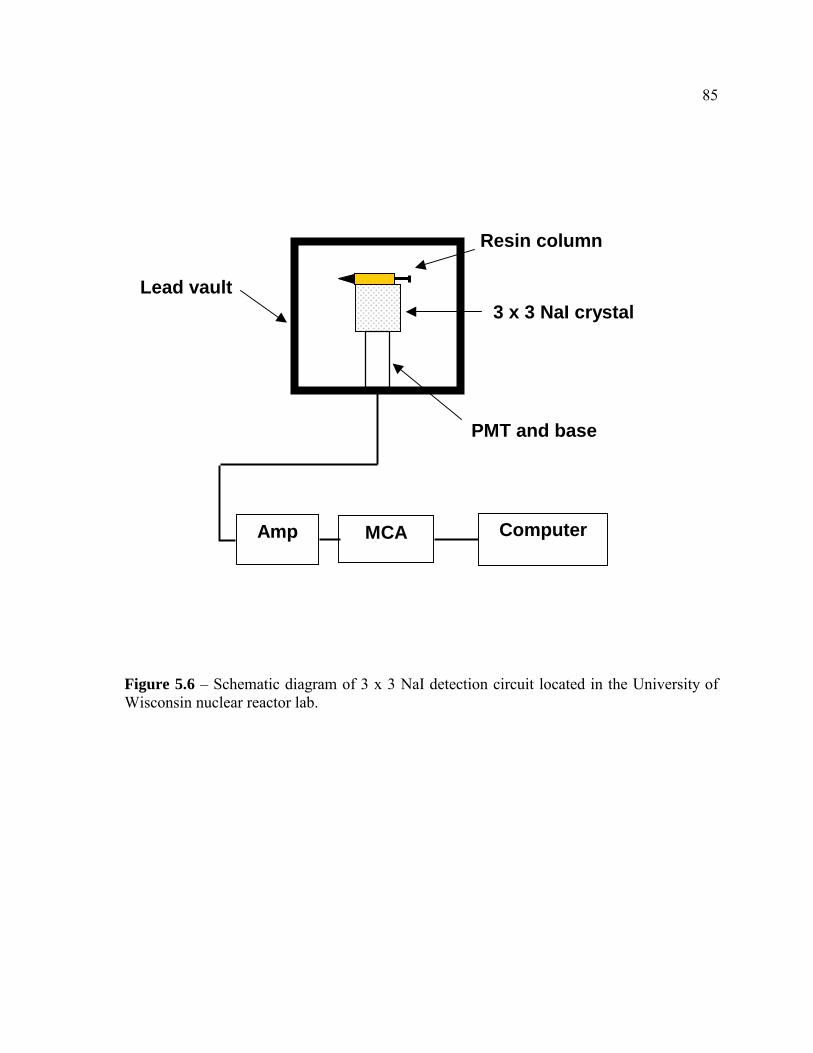
85
Computer MCA
PMT and base
3 x 3 NaI crystal
Resin column
Lead vault
Amp
Figure 5.6 – Schematic diagram of 3 x 3 NaI detection circuit located in the University of Wisconsin nuclear reactor lab.

86
Chapter 6 Experimental Results
Section 6.1 February 19th, 2003 Production Run
During the time window of operation available for this experiment, two successful
13N production runs were conducted. Many partially successful runs were also conducted
prior to and after these runs. The first successful run occurred on February 19th, 2003. For
approximately two weeks prior to this, numerous conditioning runs were done to push the
IEC operating regime to as high a voltage as achievable. During these conditioning runs, the
stalk was observed to glow as conditions approached 130 kV and 30 mA. The glowing
began at the tip of the stalk near the cathode as shown in figure 6.1, and slowly progressed
up the stalk with time. When the glowing began, the D-3He reaction rate, as measured by
the proton detector, was observed to significantly decrease in a linear manner with run time.
The impurities within the chamber significantly increased too, which was attributed to stalk
outgassing. The cathode heating pattern also transitioned from a fairly symmetric glow to a
very asymmetric glow as shown in figure 6.2. It was believed that this particular stalk
became conductive as its temperature increased. Consequently, it was drawing ion current
away from the cathode. These ions deposited their energy into the stalk, further raising the
stalk’s temperature. This increased the stalk’s conductivity, which attracted more ions. The
runaway cycle could not be overcome by manipulating the operating pressure or by reducing
the time to reach 130 kV. Despite these adverse operating characteristics, 13N production
runs were conducted due to the limited time window for experimentation.
The experiment was prepared as described in Chapter 5. The goal of the February
19th run was to operate at 145 kV and 35 mA for 20 minutes (~ two 13N half-lives). This
87
would produce a 13N yield approximately 75% of the saturated activity. If the chamber shut
down during this time, the experiment would be restarted as quickly as possible and the run
extended to reach a total of 20 minutes of proton bombardment. The chamber pressure was
initially set to approximately 1.4 mtorr, but it was expected to rise during the experiment due
to outgassing by the glowing stalk. The pressure would be maintained below 1.8 mtorr
during the experiment by adjusting the flow of D and 3He into the chamber.
For activity calculation purposes, the time equals zero point is defined as the time
when the IEC was turned on. It took approximately three minutes to bring the IEC up to 145
kV and 35 mA. No proton counts were taken during this time so that the software would be
ready to begin counting as soon as those conditions were achieved. The voltage and current
were allowed to vary slightly during the run. No attempt was made to keep the voltage or
current at exactly 145 kV or 30 mA since the reaction rate, not the applied voltage or
current, was the important factor. Moreover, it was felt that continually adjusting the
operating conditions contributed to arcing and other run difficulties.
The IEC ran very well during the first several minutes of the run as shown by a plot
of the raw proton counts in figure 6.3. To prevent the machine from shutting down when
significant arcing occurred, the voltage was reduced approximately 15 kV for several
seconds. Although temporarily decreasing the voltage also temporarily decreased the
reaction rate, this was much preferable to an arc that could shut down the machine for a
minute or more.
After approximately six minutes of bombardment (nine minutes into the experiment),
the stalk began to glow. As expected, the chamber pressure increased so the flow of D and
3He into the chamber was reduced. The cathode began to arc regularly, and approximately

88
10 minutes into the experiment the machine shut down. During the first attempt to start the
machine and quickly bring it back up to 145 kV and 35 mA, it shut down again. The
machine was restarted and brought to operating conditions as quickly as possible, but this
delay lasted approximately three minutes. Furthermore, as soon as the desired operating
conditions were achieved, the stalk immediately started glowing again. The next few proton
counts clearly showed that the reaction rate was steadily decreasing. It was decided to
continue the run until the raw proton counts per minute dropped below 50,000. This
occurred 22 minutes into the run. At that point, the run was manually terminated. A
summary of the operational characteristics for this run is included in table 6.1. The water
target was passed through the ion exchange resin as described in Chapter 5, and the resin
column was brought to the NaI detector in the UW nuclear reactor (UWNR) lab. The first
count of the resin column began approximately two and a half minutes after shut down.
The resin column was counted for five 180-second intervals. The data for each of
these counts is located in Appendix A of this document. Immediately after the five raw
counts were concluded, a 10-minute count of the background activity was taken. The raw
activity of each count was determined, and then the adjusted background activity was
subtracted to yield the net 13N activity. Finally, the net activity was divided by the detection
efficiency, measured to be 15%, to yield the true activity for each counting period. These
results are shown in table 6.2. A plot of the true activity for each count is shown in figure
6.4. The graph in figure 6.4 contains two curves. The black curve represents an exponential
fit of the data done using Microsoft Excel™(tm). As shown on the graph, the data is very
well defined by an exponential equation as indicated by the R2 value of 0.993. The R2 value
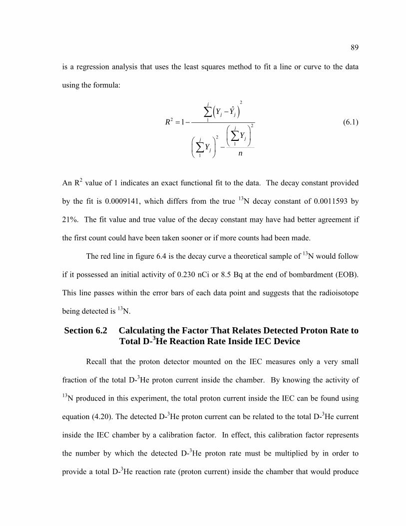
89
is a regression analysis that uses the least squares method to fit a line or curve to the data
using the formula:
� �
2
2 12
21
1
ˆ1
j
j j
j
jj
j
Y YR
YY
n
�
� �� �� �
� � � ��� �� �
�
��
(6.1)
An R2 value of 1 indicates an exact functional fit to the data. The decay constant provided
by the fit is 0.0009141, which differs from the true 13N decay constant of 0.0011593 by
21%. The fit value and true value of the decay constant may have had better agreement if
the first count could have been taken sooner or if more counts had been made.
The red line in figure 6.4 is the decay curve a theoretical sample of 13N would follow
if it possessed an initial activity of 0.230 nCi or 8.5 Bq at the end of bombardment (EOB).
This line passes within the error bars of each data point and suggests that the radioisotope
being detected is 13N.
Section 6.2 Calculating the Factor That Relates Detected Proton Rate to Total D-3He Reaction Rate Inside IEC Device
Recall that the proton detector mounted on the IEC measures only a very small
fraction of the total D-3He proton current inside the chamber. By knowing the activity of
13N produced in this experiment, the total proton current inside the IEC can be found using
equation (4.20). The detected D-3He proton current can be related to the total D-3He current
inside the IEC chamber by a calibration factor. In effect, this calibration factor represents
the number by which the detected D-3He proton rate must be multiplied by in order to
provide a total D-3He reaction rate (proton current) inside the chamber that would produce

90
the quantity of 13N that was measured. This calibration factor is calculated by first
determining the time-dependent proton current required in order to have created the quantity
of 13N produced at the end of bombardment. This is done in table 6.3 and figure 6.5. Once
the time dependent current is determined, the calibration factor relating the detected proton
rate to the total proton current required is straightforward as shown in table 6.4. From these
calculations, the calibration factor is determined to be 2,804. Thus, the number of protons
from D-3He reactions detected by the proton detector must be multiplied by 2,804 to yield
the total proton current within the IEC.
Section 6.3 February 21st, 2003 Production Run
The second successful 13N production run was conducted on February 21st, 2003.
The glowing stalk problem had grown continually worse, and high-power IEC operation was
limited to approximately 10 minutes. Nonetheless, it was believed that a measurable
quantity of 13N could be produced.
The goal of this production run was to operate at 145 kV and 35 mA for 10 minutes.
As with the first production run, the time equal zero point was defined as the moment the
IEC was turned on. The first proton count was started two minutes into the run. Due to
significant arcing, the machine shut down only four minutes into the run. After restarting
the IEC, the arcing persisted. This significantly reduced the detected proton rate between
five and eight minutes into the run as shown in table 6.5. Although the arcing did begin to
subside nearly nine minutes into the experiment, the stalk then began to glow. To minimize
the decrease in the D-3He reaction rate, the current was increased to 35 mA. This did little
to offset the reaction rate falloff, so the voltage was increased to 145 kV, and then to 150 kV

91
a few minutes later. After 10 minutes of continuous operation, the machine was shut down.
The water target was flushed through the resin as before and rushed to the UWNR detector.
The resin column was again counted for five 180-second intervals. The specific data
for each of these counts is located in Appendix B. At the conclusion of these five counts, a
background count was conducted as previously described. Using this data, the net activity
detected for each count was determined. This was then used to calculate the true activity of
13N is the resin by dividing the net activity by the 15% detection efficiency. These
calculations are shown in table 6.6. A plot of the resulting decay curve is shown in figure
6.6. As before, two curves are included in this decay curve. The shorter, black curve is an
exponential fit of the data points using Microsoft Excel™. As noted on the graph, the R2
value of the fit is 0.975, indicating the data is well defined by an exponential equation.
More importantly, the fit yields a decay constant value of 0.0011440. This differs from the
true 13N decay constant of 0.0011593 by only 1.3%. Lastly, the red line is the decay curve a
theoretical sample of 13N would follow if it had an initial activity at EOB of 0.135 nCi. The
fit curve and theoretical decay curves lie on top of each other, providing strong evidence that
13N was created in this experiment.
As with the February 19th production run, a calibration factor is determined that
relates the detected protons current, shown in figure 6.7, to the total proton current inside the
chamber. This is done in the same manner as before, and the calculations are shown in table
6.7 and 6.8 as well as figure 6.8. This experiment yields a calibration factor of 4,088.
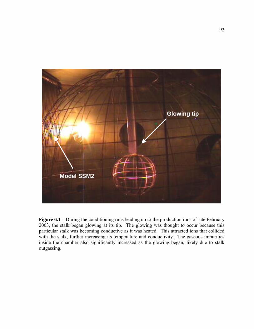
92
Model SSM2
Glowing tip
Figure 6.1 – During the conditioning runs leading up to the production runs of late February 2003, the stalk began glowing at its tip. The glowing was thought to occur because this particular stalk was becoming conductive as it was heated. This attracted ions that collided with the stalk, further increasing its temperature and conductivity. The gaseous impurities inside the chamber also significantly increased as the glowing began, likely due to stalk outgassing.

93
Figure 6.2 – The cathode heating pattern was dramatically altered as the stalk began to glow. The image on the left shows the cathode uniformly heated early in the production run on February 19th, 2003. The image on the right shows asymmetric cathode heating after the stalk began glowing. It’s thought this was caused by the stalk becoming conductive and drawing ion current away from the cathode.

94
Det
ecte
d P
roto
n C
urr
ent
Insi
de
IEC
Ch
amb
er a
s a
Fu
nct
ion
of
Ru
n T
ime
Du
rin
g t
he
Feb
ruar
y 19
th, 2
003
Pro
du
ctio
n R
un
y =
-3.
57E
-11x
+ 9
.08E
-10
R2
= 9
.58E
-01
0.E
+00
1.E
-10
2.E
-10
3.E
-10
4.E
-10
5.E
-10
6.E
-10
03
69
1215
1821
24
Irra
dia
tion
Tim
e (m
in)
Detected Proton Current (�A)
Mea
sure
d D
ata
Ave
rage
of
Dat
aLi
near
Fit
of D
ata
I =
4.6
0 E
-10 �
A
Reg
ion
1R
egio
n 2
Reg
ion
3R
egio
n 4
Figu
re 6
.3–
Plot
of
the
dete
cted
pro
ton
curr
ent a
s a
func
tion
of r
un ti
me
for
prod
uctio
n ru
n co
nduc
ted
Febr
uary
19th
, 200
3 (I
EC r
un 7
90).
The
se c
urre
nts
are
base
d on
the
det
ecte
d pr
oton
rat
e ta
ken
in o
ne-m
inut
e in
terv
als.
The
det
ecte
d pr
oton
cu
rren
t was
div
ided
into
four
regi
ons.
The
pro
ton
curr
ent i
n re
gion
1 a
nd re
gion
3 is
ass
umed
to b
e ze
ro.
The
prot
on c
urre
nt
in r
egio
n 2
is d
efin
ed to
be
a co
nsta
nt e
qual
to th
e av
erag
e of
the
curr
ent r
eadi
ng in
the
regi
on.
The
erro
r in
the
mea
sure
d pr
oton
rate
is ju
dged
to b
e 5%
in th
is re
gion
. In
regi
on 4
, a li
ne fi
t to
the
data
def
ines
the
time
depe
nden
t pro
ton
curr
ent.
The
erro
r in
the
mea
sure
d pr
oton
rate
for t
his r
egio
n is
judg
ed to
be
a co
nsta
nt 0
.5 E
-10 �
A b
ased
on
run
cond
ition
s.

95
Run Time (min)
Voltage (kV)
Current (mA)
Pressure (mtorr)
Measured D-3He
Protons/minWater Temp
(oC) 0 40 30 1.50 0 15 1 100 30 1.60 16 3 140 30 1.68 171171 20 5 145 34 1.78 182160 27 6 145 32 1.77 173589 29 8 145 31 1.80 166878 34
10 145 35 1.85 167860 11 0 0 0 12 0 0 0 13 130 30 14 145 30 1.85 159974 33 16 145 30 1.96 130195 35 17 145 33 1.72 98968 37 19 145 30 1.82 81082 40 21 145 30 1.77 68446 41 22 145 33 1.85 45940 43
Table 6.1 – Operating conditions for February 19th, 2003 isotope production run. Empty positions indicate the data was not measured for that time period. Note that the pressure increased from 1.50 mtorr to nearly 2.0 mtorr. The D and 3He flow rates were then reduced to lower the overall chamber pressure. The IEC shut down approximately 10 minutes into the run due to arcing around the cathode. The tip of the stalk began glowing at 16 minutes. The water temperature was measured using a thermocouple that was thermally cemented to the copper tube carrying the water out of the IEC chamber.

96
Cou
nt
#C
ount
Ti
me
(s)
Cou
nt S
tart
Ti
me
Afte
r EO
B (s
ec)
Gro
ss
Cts
in
180
s�
(cts
)B
kgd
Cts
in
180
s��
(cts
)N
et C
ts��
(cts
)
Net
A
ctiv
ity
(dps
)�
(dps
)Tr
ue
Act
ivity
(d
ps)
� (d
ps)
True
A
ctiv
ity
(nC
i)��(n
Ci)
118
015
626
416
.285
9.2
179
18.7
0.99
0.10
46.
630.
519
0.17
90.
014
218
034
723
415
.385
9.2
149
17.9
0.83
0.09
95.
520.
496
0.14
90.
013
318
055
021
614
.785
9.2
131
17.3
0.73
0.09
64.
850.
482
0.13
10.
013
418
075
519
013
.885
9.2
105
16.6
0.58
0.09
23.
890.
461
0.10
50.
012
518
094
517
113
.185
9.2
8616
.00.
480.
089
3.19
0.44
40.
086
0.01
2
Tab
le6.
2-
Raw
511
keV
gam
ma
ray
coun
tdat
afr
omFe
brua
ry19
thpr
oduc
tion
run.
The
time
that
elap
sed
betw
een
end
ofbo
mba
rdm
ent(
EOB
)an
dth
est
arto
fth
eea
chco
unti
slis
ted
inth
eth
irdco
lum
nfr
omth
ele
ft.Th
ene
tact
ivity
isfo
und
bysu
brac
ting
the
back
grou
ndac
tivity
(obt
aine
dfr
oma
10-m
inut
eco
unta
ndin
terp
olat
edto
a18
0-se
cond
inte
rval
)fro
mth
egr
oss
num
ber o
f cou
nts f
or th
at p
erio
d. T
he tr
ue a
ctiv
ity is
then
obt
aine
d by
div
idin
g th
e ne
t act
ivity
by
the
dete
ctio
n ef
ficie
ncy.
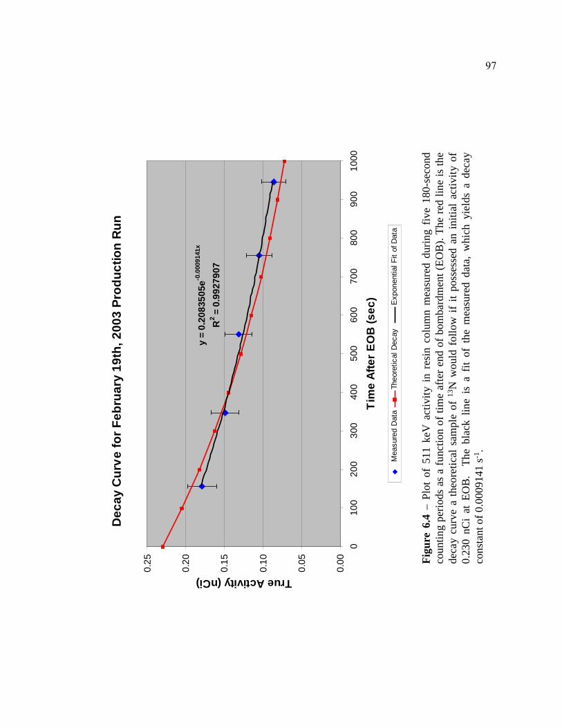
97
Dec
ay C
urve
for F
ebru
ary
19th
, 200
3 Pr
oduc
tion
Run
y =
0.20
8350
5e-0
.000
9141
x
R2 =
0.9
9279
07
0.00
0.05
0.10
0.15
0.20
0.25
010
020
030
040
050
060
070
080
090
010
00
Tim
e Af
ter E
OB
(sec
)
True Activity (nCi)
Mea
sure
d D
ata
Theo
retic
al D
ecay
E
xpon
entia
l Fit
of D
ata
Figu
re 6
.4–
Plot
of
511
keV
activ
ity i
n re
sin
colu
mn
mea
sure
d du
ring
five
180-
seco
nd
coun
ting
perio
ds a
s a
func
tion
of ti
me
afte
r end
of b
omba
rdm
ent (
EOB
). Th
e re
d lin
e is
the
deca
y cu
rve
a th
eore
tical
sam
ple
of 13
N w
ould
fol
low
if it
pos
sess
ed a
n in
itial
act
ivity
of
0.23
0 nC
iat
EO
B.
The
bla
ck l
ine
is a
fit
of t
he m
easu
red
data
, w
hich
yie
lds
a de
cay
cons
tant
of 0
.000
9141
s-1.

98
T I (uA) P (nCi) EOB A (nCi)
3.0 1.289E-06 0.793 0.211 3.5 1.289E-06 0.793 0.219 4.0 1.289E-06 0.793 0.227 4.5 1.289E-06 0.793 0.235 5.0 1.289E-06 0.793 0.243 5.5 1.289E-06 0.793 0.252 6.0 1.289E-06 0.793 0.261 6.5 1.289E-06 0.793 0.270 7.0 1.289E-06 0.793 0.279 7.5 1.289E-06 0.793 0.289 8.0 1.289E-06 0.793 0.299 8.5 1.289E-06 0.793 0.310 9.0 1.289E-06 0.793 0.321 9.5 1.289E-06 0.793 0.332 10.0 1.289E-06 0.793 0.344
14.0 1.146E-06 0.705 0.404 14.5 1.096E-06 0.674 0.400 15.0 1.046E-06 0.643 0.395 15.5 9.956E-07 0.613 0.390 16.0 9.455E-07 0.582 0.383 16.5 8.955E-07 0.551 0.376 17.0 8.454E-07 0.520 0.367 17.5 7.954E-07 0.489 0.358 18.0 7.453E-07 0.459 0.347 18.5 6.953E-07 0.428 0.335 19.0 6.452E-07 0.397 0.322 19.5 5.952E-07 0.366 0.308 20.0 5.451E-07 0.335 0.292 20.5 4.951E-07 0.305 0.274 21.0 4.450E-07 0.274 0.255 21.5 3.950E-07 0.243 0.235 22.0 3.449E-07 0.212 0.212 Potential Activity at EOB (nCi) 9.746
(9.746 nCi)(0.0236) = 0.230 nCi Table 6.3 – Table used to calculate the proton current required to produce an amount of 13N equivalent to the quantity estimated at the end of bombardment (EOB) for the production run conducted February 19th. The proton current for times between 14 and 22 minutes is found from a fit of the detected proton rate in figure 6.5. Using the values for the time-dependent flux in the table above, the potential 13N activity is calculated to be 9.746 nCi. This value is multiplied by the 0.0236 system efficiency to yield a calculated 13N activity of 0.230 nCi, which is the same as the estimated activity at EOB from the measured results in figure 6.4. This proton current then is used to calculate the calibration factor (table 6.4).
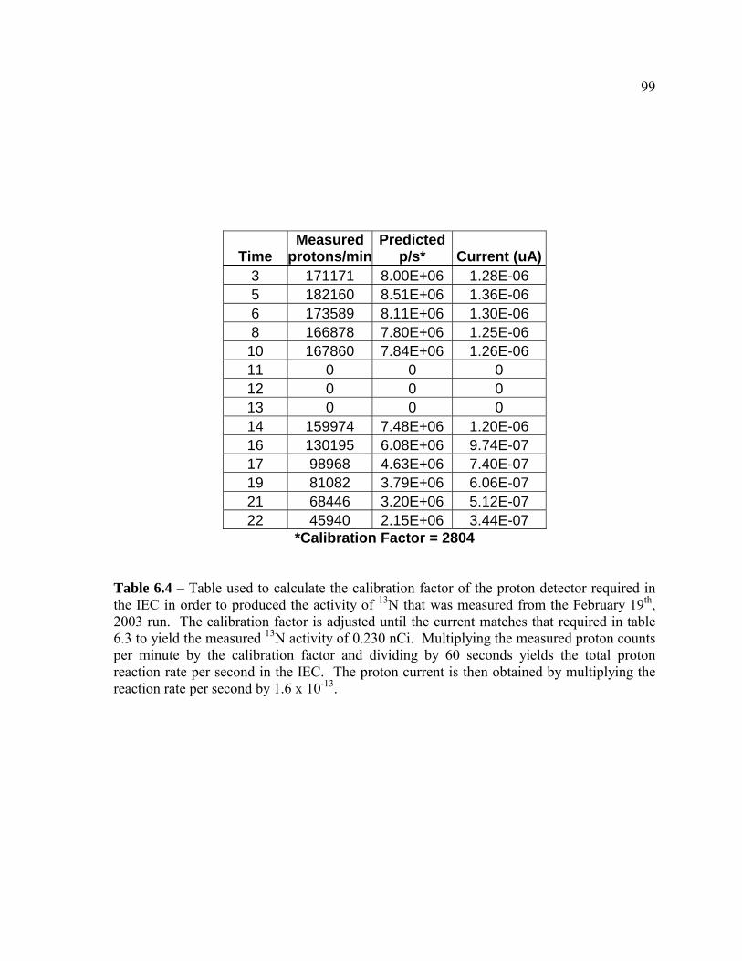
99
Time Measured
protons/minPredicted
p/s* Current (uA) 3 171171 8.00E+06 1.28E-06 5 182160 8.51E+06 1.36E-06 6 173589 8.11E+06 1.30E-06 8 166878 7.80E+06 1.25E-06
10 167860 7.84E+06 1.26E-06 11 0 0 0 12 0 0 0 13 0 0 0 14 159974 7.48E+06 1.20E-06 16 130195 6.08E+06 9.74E-07 17 98968 4.63E+06 7.40E-07 19 81082 3.79E+06 6.06E-07 21 68446 3.20E+06 5.12E-07 22 45940 2.15E+06 3.44E-07
*Calibration Factor = 2804 Table 6.4 – Table used to calculate the calibration factor of the proton detector required in the IEC in order to produced the activity of 13N that was measured from the February 19th, 2003 run. The calibration factor is adjusted until the current matches that required in table 6.3 to yield the measured 13N activity of 0.230 nCi. Multiplying the measured proton counts per minute by the calibration factor and dividing by 60 seconds yields the total proton reaction rate per second in the IEC. The proton current is then obtained by multiplying the reaction rate per second by 1.6 x 10⁻¹³.

100
Tota
l Pro
ton
Cur
rent
Req
uire
d In
side
UW
IEC
to P
rodu
ce th
e A
ctiv
ity o
f 13N
Mea
sure
d fr
om F
ebru
ary
19th
, 200
3 P
rodu
ctio
n R
un
y =
-1.0
00E
-07x
+ 2
.546
E-0
6R
2 = 9
.582
E-0
1
0.0E
+00
2.0E
-07
4.0E
-07
6.0E
-07
8.0E
-07
1.0E
-06
1.2E
-06
1.4E
-06
1.6E
-06
05
1015
2025
Irra
ditio
n T
ime
(min
)
Total Proton Current (uA)
Mea
sure
d D
ata
Ave
rage
or L
inea
r Fit
of D
ata
1.28
9E-6
�A
Figu
re 6
.5–
Plot
of t
otal
pro
ton
curr
ent n
eces
sary
insi
de th
e IE
C to
pro
duce
the
activ
ity o
f 13N
at
the
end
of b
omba
rdm
ent (
EOB
) as
estim
ated
from
figu
re 6
.4 u
sing
the
calib
ratio
n fa
ctor
of 2
,804
fr
om ta
ble
6.5.
The
ave
rage
pro
ton
curr
ent f
rom
3 to
10
min
utes
into
the
run
wou
ld n
eed
to b
e 1.
289
E-6 �
A.
From
14
to 2
2 m
inut
es, t
he p
roto
n cu
rren
t (in
�A
) is
defin
ed b
y th
e fit
equ
atio
n in
th
e fig
ure
abov
e.

101
Run Time (min)
Voltage (kV)
Current (mA)
Pressure (mtorr)
Measured D-3He
Protons/min Water Temp
(oC) 0 40 30 1.49 0 23 1 120 30 1.57 25 2 140 30 1.54 121338 31 4 140 30 1.49 0 5 140 30 1.45 141920 34 8 135 30 1.64 103132 36 9 140 30 1.68 121174 38
10 140 35 1.73 115589 39 12 140 35 1.75 89156 41 14 145 35 1.80 91994 43 15 150 35 1.96 74802 45
Table 6.5 - Operating conditions for February 21st, 2003 isotope production run. Empty positions indicated the data was not measured for that time period. The IEC shut down due to arcing approximately four minutes into the run. The stalk began glowing 10 minutes into the run, and the cathode heating became very asymmetric 12 minutes into the run. For calculation purposes, the activity of 13N created during the brief operational period two minutes into the run is neglected. Table 6.7 shows that the contribution from this brief period is only about 3% of the total 13N produced.

102
Cou
nt
#C
ount
Ti
me
(s)
Cou
nt S
tart
Ti
me
Afte
r EO
B (s
ec)
Gro
ss
Cts
in
180
s�
(cts
)B
kgd
Cts
in
180
s�
(cts
)Net
Cts
� (c
ts)
Net
A
ctiv
ity
(dps
)�
(dps
)Tr
ue
Act
ivity
(d
ps)
� (d
ps)
True
A
ctiv
ity
(nC
i)��(n
Ci)
118
022
520
014
.194
9.7
106
17.1
0.58
90.
095
3.92
60.
635
0.10
60.
017
218
041
517
213
.194
9.7
7816
.30.
433
0.09
12.
889
0.60
40.
078
0.01
63
180
615
166
12.9
949.
772
16.1
0.40
00.
090
2.66
70.
597
0.07
20.
016
418
080
514
612
.194
9.7
5215
.50.
289
0.08
61.
926
0.57
40.
052
0.01
65
180
995
137
11.7
949.
743
15.2
0.23
90.
084
1.59
30.
563
0.04
30.
015
Tab
le6.
6-
Raw
511
keV
gam
ma
ray
coun
tda
tafr
omFe
brua
ry21
stpr
oduc
tion
run.
The
time
that
elap
sed
betw
een
end
ofbo
mba
rdm
ent(
EOB
)an
dth
est
art
ofth
eea
chco
unt
islis
ted
inth
eth
irdco
lum
nfr
omth
ele
ft.Th
ene
tac
tivity
isfo
und
bysu
brac
ting
the
back
grou
ndac
tivity
(obt
aine
dfr
oma
10-m
inut
eco
unta
ndin
terp
olat
edto
a18
0-se
cond
inte
rval
)fro
mth
egr
oss
num
ber o
f cou
nts f
or th
at p
erio
d. T
he tr
ue a
ctiv
ity is
then
obt
aine
d by
div
idin
g th
e ne
t act
ivity
by
the
dete
ctio
n ef
ficie
ncy.
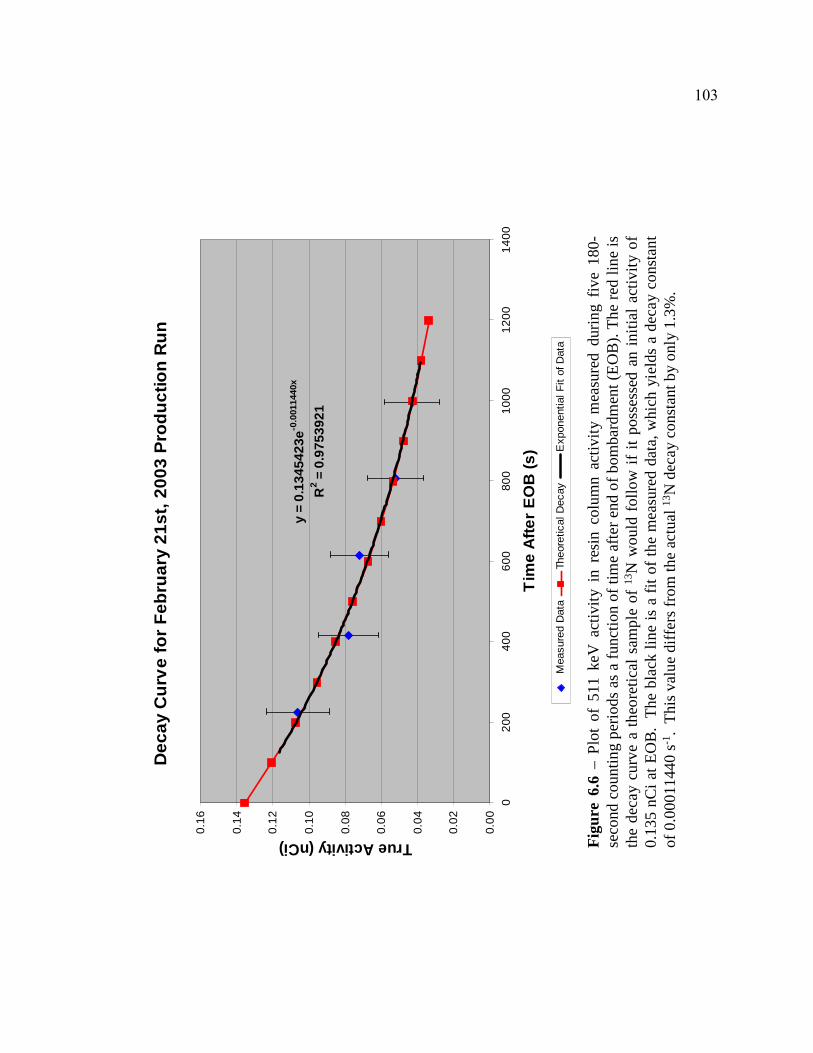
103
Dec
ay C
urve
for F
ebru
ary
21st
, 200
3 Pr
oduc
tion
Run
y =
0.13
4542
3e-0
.001
1440
x
R2 =
0.9
7539
21
0.00
0.02
0.04
0.06
0.08
0.10
0.12
0.14
0.16
020
040
060
080
010
0012
0014
00
Tim
e Af
ter E
OB
(s)
True Activity (nCi)
Mea
sure
d D
ata
Theo
retic
al D
ecay
Exp
onen
tial F
it of
Dat
a
Figu
re 6
.6–
Plot
of
511
keV
activ
ity i
n re
sin
colu
mn
activ
ity m
easu
red
durin
g fiv
e 18
0-se
cond
cou
ntin
g pe
riods
as a
func
tion
of ti
me
afte
r end
of b
omba
rdm
ent (
EOB
). Th
e re
d lin
e is
th
e de
cay
curv
e a
theo
retic
al s
ampl
e of
13N
wou
ld f
ollo
w if
it p
osse
ssed
an
initi
al a
ctiv
ity o
f 0.
135
nCia
t EO
B.
The
blac
k lin
e is
a fi
t of t
he m
easu
red
data
, whi
ch y
ield
s a
deca
y co
nsta
nt
of 0
.000
1144
0 s-1
. Th
is v
alue
diff
ers f
rom
the
actu
al 13
N d
ecay
con
stan
t by
only
1.3
%.
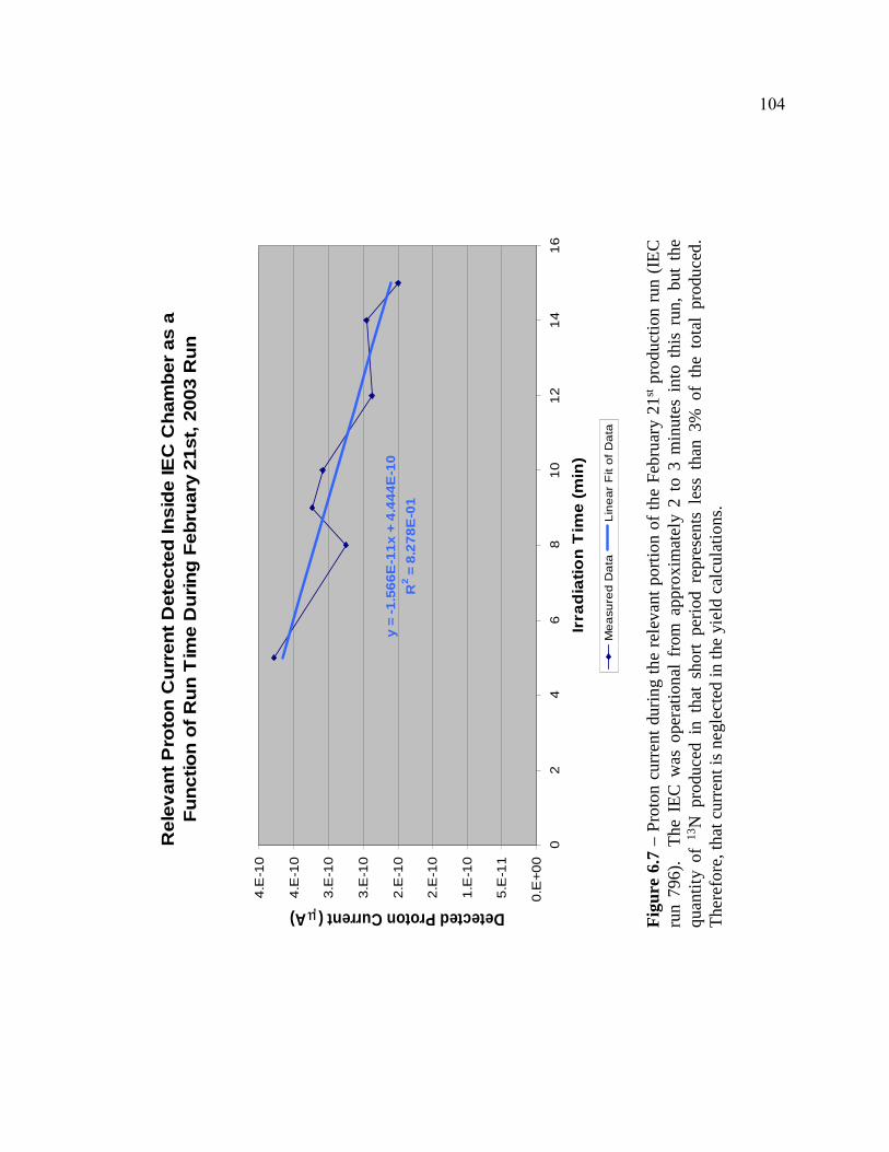
104
Rel
evan
t Pro
ton
Cur
rent
Det
ecte
d In
side
IEC
Cha
mbe
r as
a Fu
nctio
n of
Run
Tim
e D
urin
g Fe
brua
ry 2
1st,
2003
Run
y =
-1.5
66E
-11x
+ 4
.444
E-1
0R
2 = 8
.278
E-0
1
0.E
+00
5.E
-11
1.E
-10
2.E
-10
2.E
-10
3.E
-10
3.E
-10
4.E
-10
4.E
-10
02
46
810
1214
16
Irra
diat
ion
Tim
e (m
in)
Detected Proton Current (�A)
Mea
sure
d D
ata
Line
ar F
it of
Dat
a
Figu
re 6
.7–
Prot
on c
urre
nt d
urin
g th
e re
leva
nt p
ortio
n of
the
Febr
uary
21st
prod
uctio
n ru
n (I
EC
run
796)
. T
he I
EC w
as o
pera
tiona
l fr
om a
ppro
xim
atel
y 2
to 3
min
utes
int
o th
is r
un,
but
the
quan
tity
of 13
N p
rodu
ced
in t
hat
shor
t pe
riod
repr
esen
ts l
ess
than
3%
of
the
tota
l pr
oduc
ed.
Ther
efor
e, th
at c
urre
nt is
neg
lect
ed in
the
yiel
d ca
lcul
atio
ns.
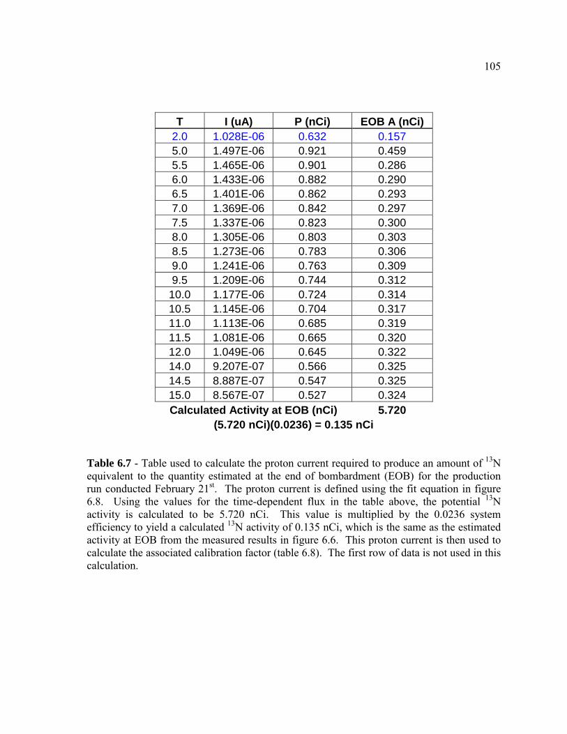
105
T I (uA) P (nCi) EOB A (nCi) 2.0 1.028E-06 0.632 0.157 5.0 1.497E-06 0.921 0.459 5.5 1.465E-06 0.901 0.286 6.0 1.433E-06 0.882 0.290 6.5 1.401E-06 0.862 0.293 7.0 1.369E-06 0.842 0.297 7.5 1.337E-06 0.823 0.300 8.0 1.305E-06 0.803 0.303 8.5 1.273E-06 0.783 0.306 9.0 1.241E-06 0.763 0.309 9.5 1.209E-06 0.744 0.312
10.0 1.177E-06 0.724 0.314 10.5 1.145E-06 0.704 0.317 11.0 1.113E-06 0.685 0.319 11.5 1.081E-06 0.665 0.320 12.0 1.049E-06 0.645 0.322 14.0 9.207E-07 0.566 0.325 14.5 8.887E-07 0.547 0.325 15.0 8.567E-07 0.527 0.324 Calculated Activity at EOB (nCi) 5.720
(5.720 nCi)(0.0236) = 0.135 nCi Table 6.7 - Table used to calculate the proton current required to produce an amount of 13N equivalent to the quantity estimated at the end of bombardment (EOB) for the production run conducted February 21st. The proton current is defined using the fit equation in figure 6.8. Using the values for the time-dependent flux in the table above, the potential 13N activity is calculated to be 5.720 nCi. This value is multiplied by the 0.0236 system efficiency to yield a calculated 13N activity of 0.135 nCi, which is the same as the estimated activity at EOB from the measured results in figure 6.6. This proton current is then used to calculate the associated calibration factor (table 6.8). The first row of data is not used in this calculation.
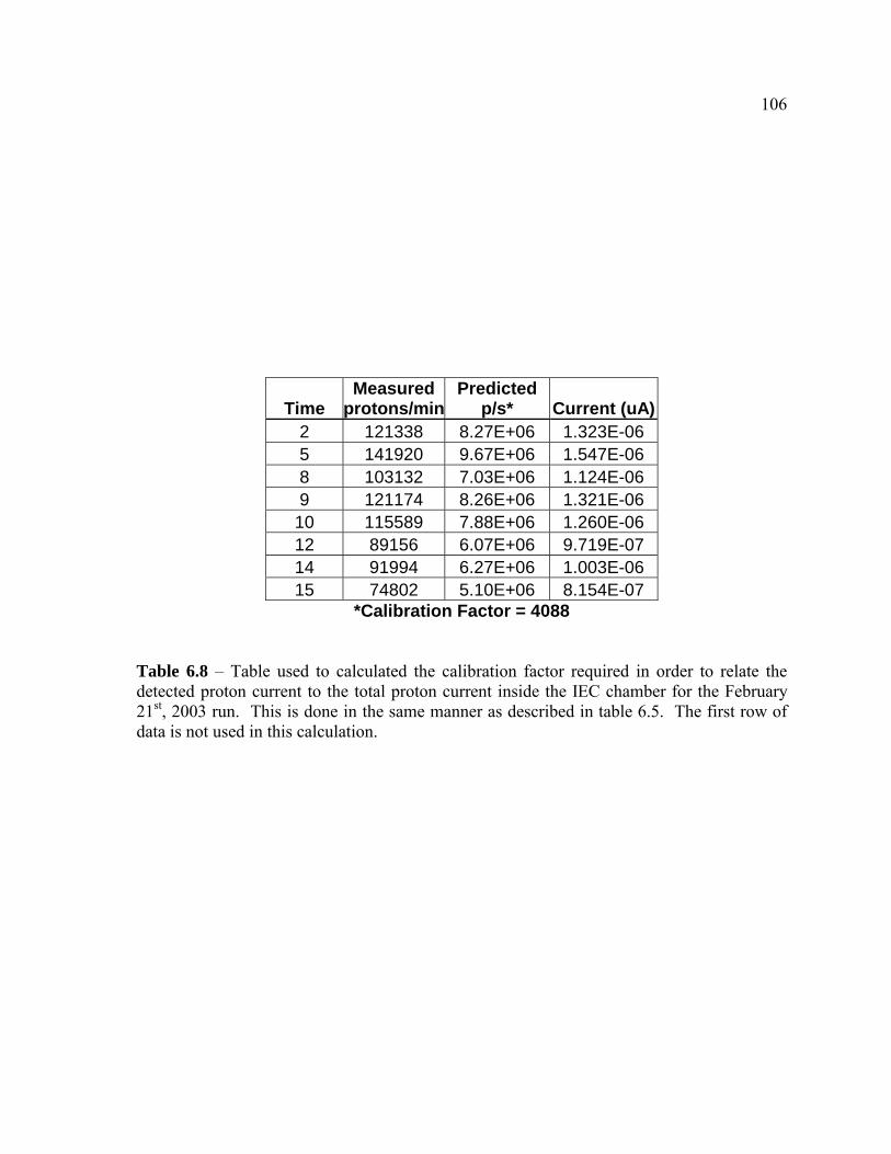
106
Time Measured
protons/minPredicted
p/s* Current (uA) 2 121338 8.27E+06 1.323E-06 5 141920 9.67E+06 1.547E-06 8 103132 7.03E+06 1.124E-06 9 121174 8.26E+06 1.321E-06
10 115589 7.88E+06 1.260E-06 12 89156 6.07E+06 9.719E-07 14 91994 6.27E+06 1.003E-06 15 74802 5.10E+06 8.154E-07
*Calibration Factor = 4088 Table 6.8 – Table used to calculated the calibration factor required in order to relate the detected proton current to the total proton current inside the IEC chamber for the February 21st, 2003 run. This is done in the same manner as described in table 6.5. The first row of data is not used in this calculation.

107
Tota
l Pro
ton
Curr
ent R
equi
red
Insi
de th
e IE
C to
Pro
duce
the
Act
ivity
of 13
N M
easu
red
from
Feb
ruar
y 21
st P
rodu
ctio
n R
un
y =
-5.6
46E-
08x
+ 1.
602E
-06
R2 =
8.2
78E-
01
0.E
+00
2.E
-07
4.E
-07
6.E
-07
8.E
-07
1.E
-06
1.E
-06
1.E
-06
2.E
-06
02
46
810
1214
16
Irrad
iatio
n Ti
me
(min
)
Proton Current (�A)
Mea
sure
d D
ata
Line
ar F
it of
Dat
a
Figu
re 6
.8–
Plot
of t
otal
pro
ton
curr
ent n
eces
sary
insi
de th
e IE
C to
pro
duce
the
activ
ity o
f 13N
at t
he e
nd
of b
omba
rdm
ent (
EOB
) as
estim
ated
from
figu
re 6
.6 u
sing
the
calib
ratio
n fa
ctor
of 4
,088
from
tabl
e 6.
8.
The
time-
depe
nden
t pro
ton
curr
ent i
s giv
en b
y th
e fit
equ
atio
n in
the
char
t abo
ve.

108
Chapter 7 Discussion of Results
Section 7.1 Certainty of Experimental Results
The true importance of the experimental results is whether or not they demonstrate
with reasonable statistical certainty that this experiment created 13N. If so, then the
experimental goal stated at the beginning of Chapter 1 was achieved. To determine this, the
error associated with each data point in figures 6.4 and 6.6 is examined. The February 19th
production run is investigated first.
As shown in table 7.1, the net number of counts detected during each of the five 180-
second count intervals from the February 19th run varies from 179 counts in the first interval
to 86 counts in the fifth interval. Since radioactive decay events follow a Poisson
distribution, the measurement uncertainty in the total net counts is calculated by summing
the uncertainty in the gross number of counts and the uncertainty in the background counts
(from table 6.2) in quadrature [7]. The statistical certainty is one minus the ratio of the
uncertainty in a count interval to the total net counts in that interval (see equation (5.1)). It
is a measure of the probability that the actual total net activity of the sample lies within the
range of the total net counts plus or minus the measurement uncertainty.
The statistical certainties from the February 19th production run range from 89.6% to
81.4%, with an average value of 86.0%. Hence, on average there is a 86% probability that
the true activity of the radioisotope measured in the ion resin lies within the error bars of
figure 6.4. Moreover, the theoretical decay curve shown in figure 6.4 passes through the
error bars of each data point. Combining these two facts creates very compelling evidence
that this experiment produced 13N.
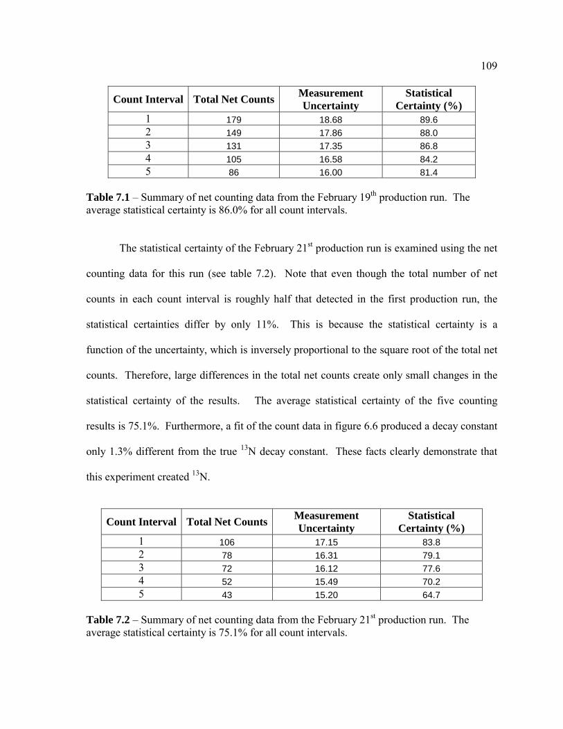
109
Count Interval Total Net Counts Measurement Uncertainty
Statistical Certainty (%)
1 179 18.68 89.6 2 149 17.86 88.0 3 131 17.35 86.8 4 105 16.58 84.2 5 86 16.00 81.4
Table 7.1 – Summary of net counting data from the February 19th production run. The average statistical certainty is 86.0% for all count intervals. The statistical certainty of the February 21st production run is examined using the net
counting data for this run (see table 7.2). Note that even though the total number of net
counts in each count interval is roughly half that detected in the first production run, the
statistical certainties differ by only 11%. This is because the statistical certainty is a
function of the uncertainty, which is inversely proportional to the square root of the total net
counts. Therefore, large differences in the total net counts create only small changes in the
statistical certainty of the results. The average statistical certainty of the five counting
results is 75.1%. Furthermore, a fit of the count data in figure 6.6 produced a decay constant
only 1.3% different from the true 13N decay constant. These facts clearly demonstrate that
this experiment created 13N.
Count Interval Total Net Counts Measurement Uncertainty
Statistical Certainty (%)
1 106 17.15 83.8 2 78 16.31 79.1 3 72 16.12 77.6 4 52 15.49 70.2 5 43 15.20 64.7
Table 7.2 – Summary of net counting data from the February 21st production run. The average statistical certainty is 75.1% for all count intervals.
110
Section 7.2 Calibration Factors
As discussed in Chapter 6, the activity of 13N produced in these two experiments
enabled the calculation of calibration factors that relate the detected D-3He proton current to
the total D-3He proton current required inside the IEC to produce the two activities of 13N
measured. These values were calculated to be 2,804 and 4,088 for the February 19th and 21st
production runs, respectively. The results of the two production experiments are deemed
equally credible, so the overall calibration factor for 13N production in the UW IEC is found
from the average of these to values. Therefore, the total proton current inside the UW IEC
is found to be a factor of 3,446 larger than the proton current measured by the proton
detector.
It is instructive to put this calibration factor into perspective. Consider the 1,200
mm2 (12cm2) surface area of the proton detector, which is located 81 cm from the center of
the cathode. The surface area of a sphere with a radius of 81 cm has a surface area of
82,448 cm2. These two surface areas differ by a factor of 6,871. If all D-3He protons were
emitted from a perfect point source in the center of the cathode and could travel isotropically
81 cm unimpeded, the proton detector would only see , of the number of protons crossing
the surface area of the sphere. The 6,871 calibration factor for this ideal case is a factor of
two larger than the 3,446 calibration factor determined above from the two 13N production
experiments. In reality, however, the D-3He protons are not emitted from an ideal point
source in the center of the cathode. A majority of the reactions likely occur on the surface of
the cathode wires [25]; some likely occur as a result of converged core reactions at the
center of the cathode; and some reactions may even be the result of a volume source

111
stemming from charge-exchange reactions. Considering this variation in the source of
protons, the 3,446 calibration factor is a reasonable value.
Section 7.3 Potential sources of Uncertainty
Throughout this experiment, several assumptions were made to simplify
measurements and calculations. Although it’s felt that these assumptions have only a very
minor effect on the resulting calculations and measurements, it’s important to note them
here for completeness. The assumptions affect two general aspects of this experiment: the
development of the theory predicting the activity of 13N created (Chapter 4), and the
measurement of the 13N activity in the resin column.
The following assumptions were made in developing the theoretical yield equations
and the system efficiencies discussed in Chapter 4. First, it was assumed that the D-3He
protons emanate from an ideal point source located in the center of the cathode. Recent
indications are that most of the D-3He protons originate from the surface of the cathode
wires [25], which span a diameter of 10 cm. Additionally, the distribution of these
embedded D-3He reactions across the length and circumference of the cathode wires is
unknown, but it is unlikely that they are uniformly distributed.
Secondly, the thickness of the stainless steel tubing is assumed to be a constant 0.013
cm. Obviously, this thickness varies within a tube and from tube to tube. The manufacturer
was unable to provide an accurate estimate of the deviation in wall thickness, but estimated
it to be 10%. Third, to determine the saturated yield the average energy lost by a proton
passing through the tube wall was calculated using an average wall thickness. A more
precise method to determine the saturated yield would be to divide the range of wall

112
thicknesses into bins and perform a weighted, numeric calculation to determine the resulting
spectrum of proton energies.
Fourth, no attempt was made to account for the effect of charge exchange reactions.
Charge exchange reactions enable fast, neutral atoms to undergo fusion reactions at
locations other than the cathode. Rather than having a proton current emanating from a
point source as assumed, the fast neutrals can create fusion reactions (and therefore proton
currents) in the volume of the chamber outside the cathode. It’s not clear what fraction of
the total D-3He fusion reactions are caused by these fast neutral atoms, but it’s thought to be
on the order of only a few percent.
Some assumptions were also made in the measurement techniques used to count the
resin column. First, the very small quantity of 13N captured by the resin column is assumed
to be located at roughly a point source near the upstream end of the column. This leads to
the second assumption, which is the detector’s efficiency in detecting the 511 keV gamma
rays from the 13N in the resin column is assumed to be the same as its efficiency in detecting
the 511 gamma rays from the small, thin, calibrated 22Na source. Third, it’s assumed that
13N is the only positron-emitting radionuclide produced in this experiment so that the decay
curve should only reflect the decay of 13N.
In summary, the results of this experiment demonstrate with a high degree of
statistical certainty that a proton current from the inertial electrostatic confinement fusion of
D-3He can repeatedly produce 13N. Moreover, the activities of 13N produced in these
experiments enabled the detected proton current to be related to the total proton current
inside the UW IEC by a factor of 3,446.

113
Chapter 8 Conclusions
The results of this proof-of-principle experiment lead to the development of the
following four major conclusions:
1) First and foremost, this experiment demonstrates that the 14.7 MeV protons
from D-3He fusion reactions in an IEC device can successfully and reproducibly create 13N.
2) Second, D-3He fusion protons from IEC fusion could create a number of
short-lived PET radioisotopes.
3) Thin-walled stainless steel tubes soldered to stainless steel manifolds can be
used to create an effective and durable water containment apparatus. Aluminum tubes do
not work well in the IEC plasma environment since electron jets easily damage them and the
joints between the tubes and manifolds could not be soldered or sealed with epoxy.
4) This experiment demonstrated that the ion exchange resin column was a
simple and efficient method to capture the 13N in a volume small enough for effective
detection.
5) Although the quantity of 13N produced in these experiments was small, this
work represents the first known demonstration of fusion technology for a commercial
purpose.

114
Chapter 9 Suggestions for Future Work
Although the quantity of 13N produced was not important for this proof-of-principle
experiment, the goals of future work in this area will surely include producing larger
activities of 13N. Larger quantities will provide longer counting times, more accurate decay
curves, and better counting statistics. Increased yields will also increase the relevance of
this work. Several improvements can be made to increase the 13N yield of this experiment.
First, the D-3He reaction rate should be increased. The 13N yield is directly
proportional to the proton current incident upon the target. Increasing the reaction rate by a
factor of 1,000 should increase the 13N yield by a factor of 1,000. Currently, the UW IEC
experimental team is developing methods to improve the IEC reaction rate using ions guns.
By using ion guns to inject a current of 3He ions into the cathode, the amount of 3He+ should
be increased. In addition, most of the background gas can be eliminated because the source
of 3He+ is external to the chamber. This will increase the mean free path of the ions and
enable them to attain higher energies within the cathode. Additionally, the research team is
investigating methods to doubly ionize the 3He, which will double its energy. The net result
should be an increase in reaction rates by a factor of 100 or more.
Second, the 13N yield can be increased by a factor of 15 or more by simply
improving the design of the water containment apparatus. If a spherical apparatus were
placed outside the cathode, the protons would strike the walls of the apparatus orthogonally
(assuming a point source of protons located in the center of the chamber). This would
eliminate the system efficiency caused by the round tube geometry. If this apparatus
intercepted 90% of the D-3He protons produced, the efficiency of the isotope production

115
system defined in Chapter 4 would increase from 0.0236 to 0.3727 – nearly a factor of 16
greater.
Third, the proton current must remain constant throughout an isotope production run.
During the two production runs conducted in this experiment, the D-3He reaction rate
decrease in a linear fashion after only a few minutes IEC operation. The proton currents at
the end of the production runs were less than half of their initial value. It’s believed the
stalk caused this phenomenon to occur. Therefore, improvements must be made to the stalk
and, if necessary, the cathode to ensure the IEC can maintain a constant fusion reaction rate
for 15 minutes or more.
Fourth, better detection systems should be used to count the 511 keV gamma
ray activity of the resin column. Although much less efficient, a coincidence detection
system can reduce the background activity by a factor of several hundred. This might allow
small-activity samples to be counted for longer periods of time. Additionally, well counters
should be used in order to vastly improve the detection efficiency.
Finally, a 13C target could be used to create 13N from (p,n) reactions. Although very
expensive (currently ~$250/g), the saturated yield from 13C is approximately seven times
larger than the saturated yield of water. A 13C target also poses the additional problem of
13N extraction, but Dr. Andy Roberts of the University of Wisconsin Department of Medical
Physics has developed techniques to sweep solid carbon targets with hydrogen gas in order
to produce 13N-amonnia. The efficiency of this process is thought to be about 20% and new
methods are being investigated that should further increase this.

116
References [1] IAEA, Charged-particle Cross Section Database for Medical Radioisotope Production
[Electronic version]. IAEA-TECDOC-1211 (May 2001). [2] R.J. Nickles, “The Production of a Broader Palette of PET Tracers,” Journal of
Labelled Compounds and Radiopharmaceuticals 45, 1 (2002). [3] Centers for Medicare and Medicaid Services, Department of Health and Human
Serives, (August 16th, 2003), Retrieved April 29, 2003 from Centers for Medicare and Medicaid Web site: http://www.cms.hhs.gov/ncdr/memo.asp?id=66
[4] K. Becker, Photographic Film Dosimetry: Principles and Methods of Quantitative
Measurement of Radiation by Photographic Means, pp. 13-15, Focal P., London, (1966).
[5] J.A. Sorenson and M.E. Phelps, Physics in Nuclear Medicine, 2nd ed., pp. 434-451,
W.B. Saunders Company, Philadelphia, (1987). [6] R.D. Evans, The Atomic Nucleus, pp. 629-630, McGraw-Hill, New York, (1955). [7] C. Knoll, Radiation Detection and Measurement, 3rd ed., pp. 65-97, 335-341, 668-680,
John Wiley & Sons, Inc., New York, (2000). [8] N. Tamaki, et al., “Dynamic Positron Computed Tomography of the Heart with a High
Sensitivity Positron Camera and Nitrogen-13 Ammonia,” Journal of Nuclear Medicine 26, 567 (1985).
[9] P.V. Harper, et al., “Clinical Feasibility of Myocardial Imaging with 13NH3,” Journal
of Nuclear Medicine 13, 278 (1972). [10] W.G. Kuhle, et al., “Quantification of Regional Myocardial Blood Flow Using 13N
Ammonia and Reoriented Dynamic Positron Emission Tomographic Imaging,” Circulation 86, 1004 (1992).
[11] O. Muzik, et al., “Validation of Nitrogen-13-ammonia Tracer Kinetic Model for
Quantification of Myocardial Blood Flow Using PET,” Journal of Nuclear Medicine, 34, 83 (1993).
[12] G.H. Miley, et al., “Inertial –Electrostatic Confinement: An Approach to Burning
Advanced Fuels,” Fusion Technology 19, 840 (1991) [13] P.T. Farnsworth, “Method and Apparatus for Producting Nuclear-Fusion Reactions,”
U.S. Patent #3,386,883 (1968)

117
[14] R.L. Hirsch, “Inertial-Electrostatic Confinement of Ionized Fuions Gases,” Journal of
Applied Physics 38, 4522 (1967). [15] R.W. Bussard, “Some Phyics Considerations of Magnetic Inertial-Electrostatic
Confinement: A New Concept for Spherical Converging-Flow Fusion,” Fusion Technology 19, 273 (1991)
[16] G.L. Kulcinski, “The United States IEC Program,” Fifth U.S.-Japan Workshop on
Inertial Electrostatic Confinement Fusion, University of Wisconsin – Madison, October 9-10, 2002.
[17] L.J. Wittenberg, J.F. Santarius, and G.L. Kulcinski, “Lunar Sources of 3He for
Commercial Fusion Power,” Fusion Technology 10 2, 167 (1986). [18] K.R. Harris-Kuhlman, “Trapping and Diffusion of Helium in Lunar Materials,” Ph.D.
Thesis, University of Wisconsin – Madison, (1998). [19] G.L. Kulcinski, “Near Term Commercial Opportunities from Long Range Fusion
Research,” Fusion Technology 30, 411 (1996). [20] G.L. Kulcinski, and H.H. Schmitt, “Fusion Power from Lunar Resources,” Fusion
Technology 21, 2221 (1992). [21] G.L. Kulcinski and J.F. Santarius, “New Opportunities for Fusion in the 21st Century –
Advanced Fuels,” Fusion Technology 39, 480 (2001). [22] G.L. Kulcinski, “Non-Electric Applications of Fusion Energy – An Important
Precursor to Commercial Electric Power,” Fusion Technology 34, 477 (1998). [23] G.L. Kulcinski, I.N. Sviatoslavsky, G.A. Emmert, H.M. Attaya, J.F. Santarius, M.E.
Sawan, and Z. Musicki, “The commercial Potential of D-He3 Fusion Reactors,” 12th Symposium on Fusion Engineering, Monterey, CA, IEEE Cat. No. 87CH2507-2, Vol. 1, p. 772 (1987).
[24] R.P. Ashley, G.L. Kulcinski, J.F. Santarius, S. Krupakar Murali, G. Piefer, and R.
Radel, “Steady-State D-3He Proton Production in an IEC Fusion Device,” Fusion Technology 39, (2001).
[25] B.B. Cipiti, and G.L. Kulcinski, “Embedded D-3He Fusion Reactions and Medical
isotope production in an Intertial Electrostatic Confinement Device,” 15th Topical Meeting of Fusion Energy, American Nuclear Society, Washington, D.C., November 17-21, 2002.

118
[26] K. Dorfner, Editor, Ion Exchangers, pp. 14-112, Walter de Gruyter & Co., Berlin, (1990).
[27] National Institute of Standards and Technologies PSTAR program,
http://physics.nist.gov/PhysRefData/Star/Text/PSTAR.html, February, 2002. [28] H.Y. Khater, “Activation and Safety Analysis for Advanced Fuel Fusion Reactors,”
Ph.D. Thesis, University of Wisconsin – Madison, (1990). [29] N.N. Krasnov, “Thick Target Yield,” International Journal of Applied Radiation and
Isotopes 25, 223 (1974). [30] K. Svoboda, “Terms Used in the Production of Radioisotopes by Charged-Particle
Bombardment,” The Use of Cyclotrons in Chemistry, Metallurgy and Biology, p. 383, Butterworths, London (1970).
[31] J. Lange and H. Munzel, “Estimation of Unknown Excitation Functions for (xn),
(pxn), (d,xn) and (p,xn) Reactions,” Kernforschungszentrum Karlsruhe, KFK-767 (May, 1968).
[32] N.N. Krasnov, “Physical Principles of Activation Analysis with Charged Particles,”
Atomnaya Energiya 26, 3 (1969). [33] K.A. Keller, J. Lange and H. Munzel, “Numerical Data and Functional Relationships
in Science and Technology,” Landolt-Bornstein, New Series, Vol I/5C, Springer (1974).
[34] J. Stewart, Calculus: Early Transcendentals, 3rd ed., pp. 340-341, Brooks/Cole, Pacific
Grove, CA., (1995). [35] F.H. Attix, Introduction to Radiological Physics and Radiation Dosimetry, pp. 560,
John Wiley and Sons, New York, (1986).

119
Appendix A Raw Count Data from February 19th, 2003 Isotope Production Run
Raw 511 keV gamma ray measurements of resin column from first 180-second
count. Although the MCA capable of detecting events up to energies of 5 MeV, no
significant number of counts were detected above 1 MeV during these measurement.
Energy (keV) Raw Counts
in 180 s Energy (keV)Raw Counts in
180 s Energy (keV) Raw Counts
in 180 s 0.0 46 327.3 11 663.8 7 0.9 40 337.5 12 674.0 4 11.1 40 347.7 16 684.2 3 21.3 46 357.9 8 694.4 7 31.5 60 368.1 14 704.6 5 41.7 60 378.3 18 714.8 6 51.9 60 388.5 15 725.0 8 62.1 45 398.7 8 735.2 2 72.3 29 408.9 8 745.4 7 82.5 23 419.1 11 755.6 5 92.7 19 429.3 12 765.8 1 102.9 25 439.5 12 776.0 7 113.1 12 449.7 13 786.2 6 123.3 23 459.9 20 796.4 7 133.5 31 470.1 23 806.6 2 143.7 27 480.2 22 816.8 6 153.9 27 490.4 36 827.0 7 164.1 29 500.6 38 837.2 7 174.3 22 510.8 40 847.4 6 184.5 26 521.0 26 857.6 4 194.7 24 531.2 21 867.8 3 204.9 23 541.4 18 878.0 3 215.1 24 551.6 12 888.2 5 225.3 16 561.8 8 898.4 6 235.5 23 572.0 5 908.6 0 245.7 12 582.2 12 918.8 5 255.9 13 592.4 5 929.0 8 266.1 15 602.6 15 939.2 1 276.3 11 612.8 7 949.4 4 286.5 23 623.0 2 959.6 4 296.7 16 633.2 4 969.8 4 306.9 10 643.4 5 980.0 5 317.1 11 653.6 8 990.2 4

120
Raw count data from second 180-second count.
Energy (keV)
Raw Counts in
180 s Energy (keV)
Raw Counts in
180 s Energy (keV)
Raw Counts in
180 s 0.0 46 327.3 14 663.8 7 0.9 36 337.5 13 674.0 7 11.1 42 347.7 11 684.2 12 21.3 45 357.9 12 694.4 6 31.5 52 368.1 9 704.6 6 41.7 57 378.3 19 714.8 9 51.9 51 388.5 12 725.0 5 62.1 46 398.7 12 735.2 7 72.3 32 408.9 10 745.4 2 82.5 19 419.1 15 755.6 12 92.7 15 429.3 8 765.8 8 102.9 13 439.5 14 776.0 6 113.1 12 449.7 14 786.2 4 123.3 20 459.9 19 796.4 3 133.5 22 470.1 22 806.6 5 143.7 27 480.2 21 816.8 4 153.9 21 490.4 33 827.0 4 164.1 18 500.6 35 837.2 5 174.3 20 510.8 33 847.4 3 184.5 18 521.0 26 857.6 6 194.7 20 531.2 21 867.8 3 204.9 20 541.4 12 878.0 3 215.1 28 551.6 6 888.2 5 225.3 18 561.8 6 898.4 5 235.5 22 572.0 13 908.6 6 245.7 18 582.2 10 918.8 7 255.9 15 592.4 4 929.0 2 266.1 23 602.6 10 939.2 4 276.3 25 612.8 9 949.4 2 286.5 10 623.0 11 959.6 5 296.7 14 633.2 10 969.8 6 306.9 12 643.4 9 980.0 5 317.1 13 653.6 3 990.2 3
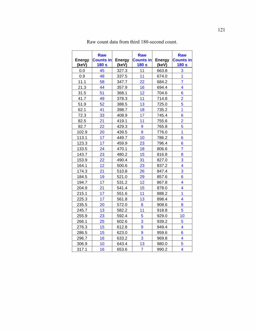
121
Raw count data from third 180-second count.
Energy (keV)
Raw Counts in
180 s Energy (keV)
Raw Counts in
180 s Energy (keV)
Raw Counts in
180 s 0.0 45 327.3 11 663.8 3 0.9 48 337.5 11 674.0 1 11.1 58 347.7 22 684.2 7 21.3 44 357.9 16 694.4 4 31.5 51 368.1 12 704.6 6 41.7 49 378.3 11 714.8 2 51.9 52 388.5 13 725.0 5 62.1 41 398.7 18 735.2 1 72.3 33 408.9 17 745.4 6 82.5 21 419.1 11 755.6 2 92.7 22 429.3 9 765.8 5 102.9 20 439.5 9 776.0 1 113.1 17 449.7 10 786.2 6 123.3 17 459.9 23 796.4 6 133.5 24 470.1 18 806.6 7 143.7 23 480.2 15 816.8 8 153.9 22 490.4 31 827.0 3 164.1 12 500.6 23 837.2 4 174.3 21 510.8 26 847.4 3 184.5 19 521.0 29 857.6 6 194.7 17 531.2 12 867.8 4 204.9 21 541.4 15 878.0 4 215.1 17 551.6 11 888.2 1 225.3 17 561.8 13 898.4 4 235.5 20 572.0 8 908.6 8 245.7 13 582.2 11 918.8 5 255.9 23 592.4 5 929.0 10 266.1 25 602.6 3 939.2 5 276.3 15 612.8 9 949.4 4 286.5 15 623.0 9 959.6 6 296.7 16 633.2 3 969.8 4 306.9 10 643.4 13 980.0 5 317.1 16 653.6 7 990.2 4

122
Raw count data from fourth 180-second count.
Energy (keV)
Raw Counts in
180 s Energy (keV)
Raw Counts in
180 s Energy (keV)
Raw Counts in
180 s 0.0 45 327.3 13 663.8 6 0.9 36 337.5 17 674.0 7 11.1 45 347.7 14 684.2 7 21.3 55 357.9 11 694.4 4 31.5 59 368.1 10 704.6 4 41.7 45 378.3 12 714.8 4 51.9 56 388.5 14 725.0 5 62.1 30 398.7 11 735.2 6 72.3 23 408.9 13 745.4 3 82.5 23 419.1 15 755.6 3 92.7 18 429.3 14 765.8 5 102.9 17 439.5 7 776.0 3 113.1 16 449.7 10 786.2 5 123.3 20 459.9 14 796.4 5 133.5 22 470.1 17 806.6 4 143.7 24 480.2 19 816.8 5 153.9 29 490.4 24 827.0 10 164.1 25 500.6 24 837.2 2 174.3 23 510.8 30 847.4 5 184.5 25 521.0 17 857.6 5 194.7 21 531.2 18 867.8 3 204.9 16 541.4 10 878.0 8 215.1 19 551.6 9 888.2 4 225.3 15 561.8 8 898.4 5 235.5 19 572.0 5 908.6 4 245.7 18 582.2 8 918.8 4 255.9 14 592.4 9 929.0 6 266.1 20 602.6 9 939.2 7 276.3 18 612.8 9 949.4 1 286.5 16 623.0 8 959.6 2 296.7 9 633.2 5 969.8 4 306.9 20 643.4 5 980.0 1 317.1 11 653.6 7 990.2 3

123
Raw count data from fifth 180-second count.
Energy (keV)
Raw Counts in
180 s Energy (keV)
Raw Counts in
180 s Energy (keV)
Raw Counts in
180 s 0.0 30 327.3 18 663.8 4 0.9 46 337.5 10 674.0 3 11.1 45 347.7 19 684.2 7 21.3 48 357.9 16 694.4 2 31.5 52 368.1 11 704.6 5 41.7 48 378.3 11 714.8 6 51.9 52 388.5 13 725.0 3 62.1 38 398.7 9 735.2 6 72.3 20 408.9 9 745.4 5 82.5 21 419.1 19 755.6 4 92.7 18 429.3 7 765.8 8 102.9 20 439.5 12 776.0 4 113.1 19 449.7 18 786.2 3 123.3 21 459.9 17 796.4 6 133.5 19 470.1 16 806.6 4 143.7 20 480.2 13 816.8 4 153.9 27 490.4 13 827.0 5 164.1 29 500.6 30 837.2 4 174.3 24 510.8 20 847.4 2 184.5 19 521.0 15 857.6 4 194.7 22 531.2 17 867.8 3 204.9 12 541.4 5 878.0 3 215.1 19 551.6 16 888.2 6 225.3 24 561.8 9 898.4 4 235.5 14 572.0 13 908.6 4 245.7 21 582.2 3 918.8 2 255.9 11 592.4 8 929.0 5 266.1 11 602.6 11 939.2 2 276.3 11 612.8 9 949.4 5 286.5 11 623.0 8 959.6 7 296.7 13 633.2 4 969.8 3 306.9 8 643.4 8 980.0 5 317.1 15 653.6 8 990.2 9

124
Appendix B Raw Count Data from February 21st, 2003 Isotope Production Run
Raw 511 keV gamma ray measurements of resin column from first 180-second
count. Although the MCA capable of detecting events up to energies of 5 MeV, no
significant number of counts were detected above 1 MeV during these measurement.
Energy (keV)
Raw Counts in
180 s Energy (keV)
Raw Counts in
180 s Energy (keV)
Raw Counts in
180 s 0.0 44 327.3 6 663.8 3 0.9 42 337.5 14 674.0 3 11.1 44 347.7 6 684.2 3 21.3 60 357.9 14 694.4 7 31.5 61 368.1 14 704.6 7 41.7 40 378.3 9 714.8 3 51.9 53 388.5 9 725.0 4 62.1 34 398.7 9 735.2 3 72.3 27 408.9 9 745.4 3 82.5 20 419.1 8 755.6 8 92.7 19 429.3 14 765.8 4 102.9 21 439.5 10 776.0 5 113.1 17 449.7 12 786.2 3 123.3 25 459.9 10 796.4 6 133.5 18 470.1 18 806.6 4 143.7 18 480.2 20 816.8 3 153.9 29 490.4 28 827.0 6 164.1 22 500.6 22 837.2 6 174.3 32 510.8 28 847.4 6 184.5 20 521.0 29 857.6 5 194.7 17 531.2 16 867.8 4 204.9 15 541.4 12 878.0 5 215.1 22 551.6 10 888.2 5 225.3 16 561.8 7 898.4 3 235.5 20 572.0 11 908.6 2 245.7 15 582.2 5 918.8 5 255.9 23 592.4 8 929.0 4 266.1 14 602.6 8 939.2 3 276.3 19 612.8 5 949.4 3 286.5 20 623.0 11 959.6 2 296.7 17 633.2 3 969.8 7 306.9 15 643.4 4 980.0 4 317.1 18 653.6 9 990.2 5
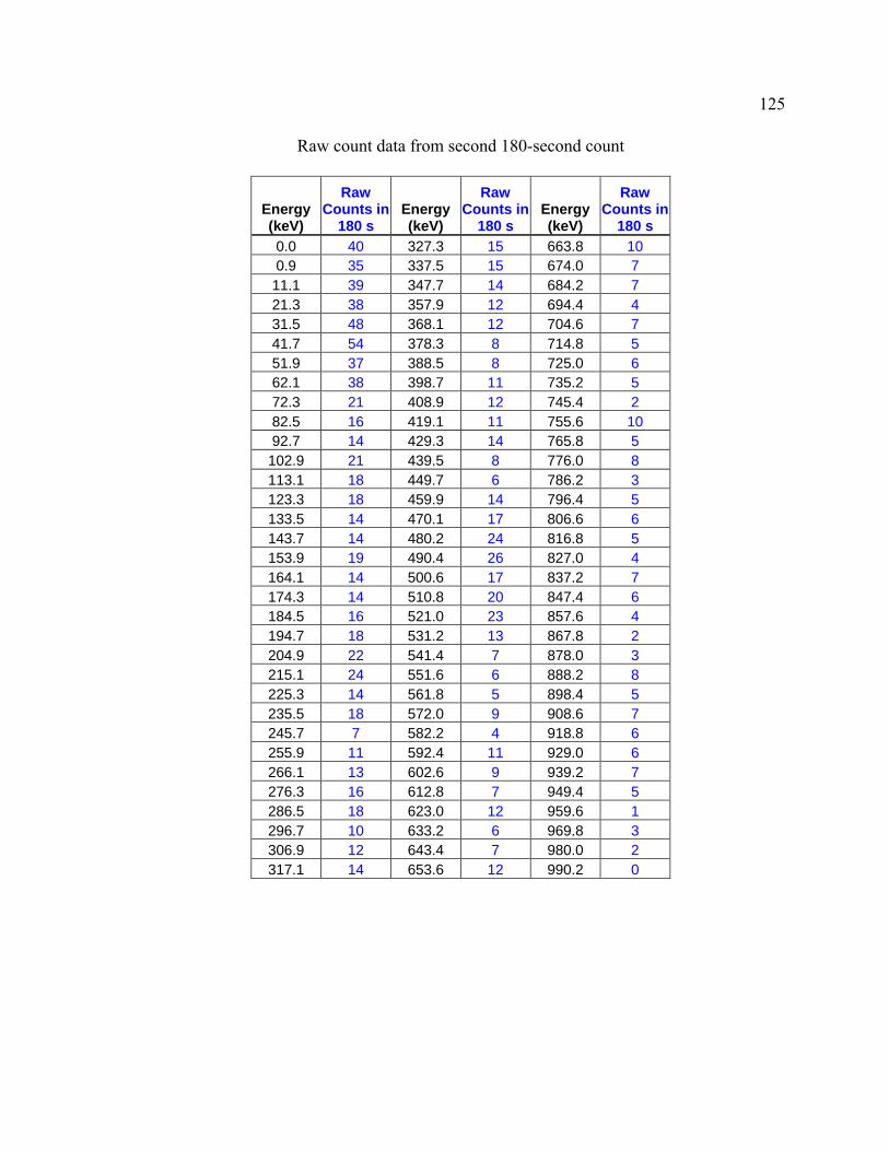
125
Raw count data from second 180-second count
Energy (keV)
Raw Counts in
180 s Energy (keV)
Raw Counts in
180 s Energy (keV)
Raw Counts in
180 s 0.0 40 327.3 15 663.8 10 0.9 35 337.5 15 674.0 7 11.1 39 347.7 14 684.2 7 21.3 38 357.9 12 694.4 4 31.5 48 368.1 12 704.6 7 41.7 54 378.3 8 714.8 5 51.9 37 388.5 8 725.0 6 62.1 38 398.7 11 735.2 5 72.3 21 408.9 12 745.4 2 82.5 16 419.1 11 755.6 10 92.7 14 429.3 14 765.8 5 102.9 21 439.5 8 776.0 8 113.1 18 449.7 6 786.2 3 123.3 18 459.9 14 796.4 5 133.5 14 470.1 17 806.6 6 143.7 14 480.2 24 816.8 5 153.9 19 490.4 26 827.0 4 164.1 14 500.6 17 837.2 7 174.3 14 510.8 20 847.4 6 184.5 16 521.0 23 857.6 4 194.7 18 531.2 13 867.8 2 204.9 22 541.4 7 878.0 3 215.1 24 551.6 6 888.2 8 225.3 14 561.8 5 898.4 5 235.5 18 572.0 9 908.6 7 245.7 7 582.2 4 918.8 6 255.9 11 592.4 11 929.0 6 266.1 13 602.6 9 939.2 7 276.3 16 612.8 7 949.4 5 286.5 18 623.0 12 959.6 1 296.7 10 633.2 6 969.8 3 306.9 12 643.4 7 980.0 2 317.1 14 653.6 12 990.2 0

126
Raw count data from third 180-second count
Energy (keV)
Raw Counts in
180 s Energy (keV)
Raw Counts in
180 s Energy (keV)
Raw Counts in
180 s 0.0 36 327.3 8 663.8 4 0.9 33 337.5 13 674.0 4 11.1 49 347.7 11 684.2 9 21.3 52 357.9 16 694.4 4 31.5 44 368.1 11 704.6 6 41.7 35 378.3 9 714.8 6 51.9 32 388.5 12 725.0 8 62.1 29 398.7 7 735.2 3 72.3 31 408.9 12 745.4 13 82.5 24 419.1 2 755.6 6 92.7 14 429.3 7 765.8 5 102.9 20 439.5 6 776.0 9 113.1 13 449.7 13 786.2 7 123.3 15 459.9 15 796.4 7 133.5 19 470.1 8 806.6 6 143.7 27 480.2 14 816.8 3 153.9 17 490.4 29 827.0 3 164.1 29 500.6 22 837.2 6 174.3 20 510.8 21 847.4 7 184.5 20 521.0 14 857.6 3 194.7 24 531.2 12 867.8 6 204.9 17 541.4 18 878.0 2 215.1 17 551.6 9 888.2 6 225.3 19 561.8 4 898.4 7 235.5 17 572.0 7 908.6 4 245.7 19 582.2 9 918.8 4 255.9 12 592.4 8 929.0 4 266.1 8 602.6 7 939.2 9 276.3 17 612.8 7 949.4 4 286.5 13 623.0 8 959.6 7 296.7 14 633.2 7 969.8 5 306.9 21 643.4 8 980.0 3 317.1 6 653.6 6 990.2 2
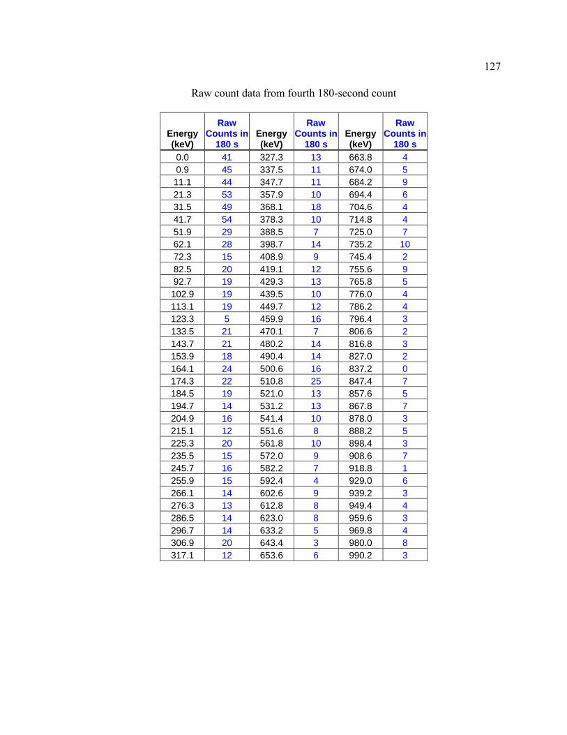
127
Raw count data from fourth 180-second count
Energy (keV)
Raw Counts in
180 s Energy (keV)
Raw Counts in
180 s Energy (keV)
Raw Counts in
180 s 0.0 41 327.3 13 663.8 4 0.9 45 337.5 11 674.0 5 11.1 44 347.7 11 684.2 9 21.3 53 357.9 10 694.4 6 31.5 49 368.1 18 704.6 4 41.7 54 378.3 10 714.8 4 51.9 29 388.5 7 725.0 7 62.1 28 398.7 14 735.2 10 72.3 15 408.9 9 745.4 2 82.5 20 419.1 12 755.6 9 92.7 19 429.3 13 765.8 5 102.9 19 439.5 10 776.0 4 113.1 19 449.7 12 786.2 4 123.3 5 459.9 16 796.4 3 133.5 21 470.1 7 806.6 2 143.7 21 480.2 14 816.8 3 153.9 18 490.4 14 827.0 2 164.1 24 500.6 16 837.2 0 174.3 22 510.8 25 847.4 7 184.5 19 521.0 13 857.6 5 194.7 14 531.2 13 867.8 7 204.9 16 541.4 10 878.0 3 215.1 12 551.6 8 888.2 5 225.3 20 561.8 10 898.4 3 235.5 15 572.0 9 908.6 7 245.7 16 582.2 7 918.8 1 255.9 15 592.4 4 929.0 6 266.1 14 602.6 9 939.2 3 276.3 13 612.8 8 949.4 4 286.5 14 623.0 8 959.6 3 296.7 14 633.2 5 969.8 4 306.9 20 643.4 3 980.0 8 317.1 12 653.6 6 990.2 3
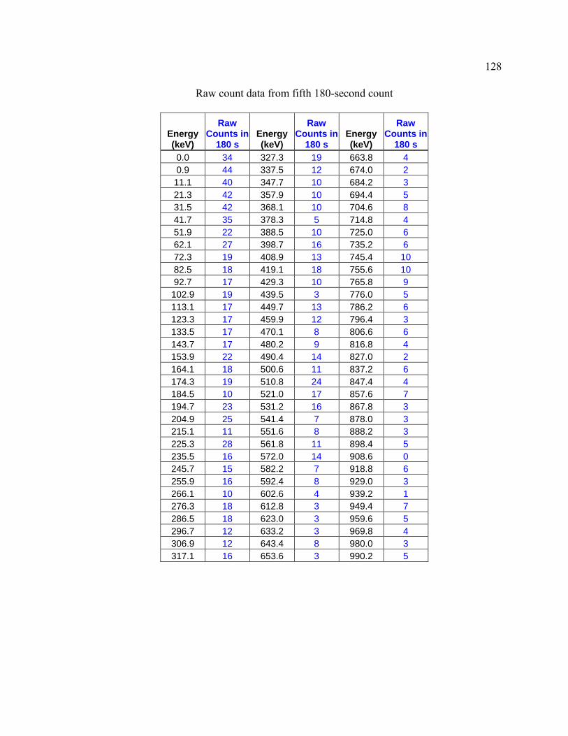
128
Raw count data from fifth 180-second count
Energy (keV)
Raw Counts in
180 s Energy (keV)
Raw Counts in
180 s Energy (keV)
Raw Counts in
180 s 0.0 34 327.3 19 663.8 4 0.9 44 337.5 12 674.0 2 11.1 40 347.7 10 684.2 3 21.3 42 357.9 10 694.4 5 31.5 42 368.1 10 704.6 8 41.7 35 378.3 5 714.8 4 51.9 22 388.5 10 725.0 6 62.1 27 398.7 16 735.2 6 72.3 19 408.9 13 745.4 10 82.5 18 419.1 18 755.6 10 92.7 17 429.3 10 765.8 9 102.9 19 439.5 3 776.0 5 113.1 17 449.7 13 786.2 6 123.3 17 459.9 12 796.4 3 133.5 17 470.1 8 806.6 6 143.7 17 480.2 9 816.8 4 153.9 22 490.4 14 827.0 2 164.1 18 500.6 11 837.2 6 174.3 19 510.8 24 847.4 4 184.5 10 521.0 17 857.6 7 194.7 23 531.2 16 867.8 3 204.9 25 541.4 7 878.0 3 215.1 11 551.6 8 888.2 3 225.3 28 561.8 11 898.4 5 235.5 16 572.0 14 908.6 0 245.7 15 582.2 7 918.8 6 255.9 16 592.4 8 929.0 3 266.1 10 602.6 4 939.2 1 276.3 18 612.8 3 949.4 7 286.5 18 623.0 3 959.6 5 296.7 12 633.2 3 969.8 4 306.9 12 643.4 8 980.0 3 317.1 16 653.6 3 990.2 5