Embed Size (px)
Citation preview
2005/09/23 Oulu, Finland
UWB Double-Directional Channel Sounding
- Why and how? -
Jun-ichi TakadaTokyo Institute of Technology, Japan

Table of Contents
• Background and motivation• Antennas and propagation in UWB• UWB double directional channel sounding
system• Parametric multipath modeling for UWB• ML-based parameter estimation• Examples

UWB Systems
• Low power – Short range
• Location awareness– High resolution in time domain
• Example applications– IEEE 802.15.3a : high speed PAN– IEEE 802.15.4a : low speed and location
aware – Ground penetrating radar
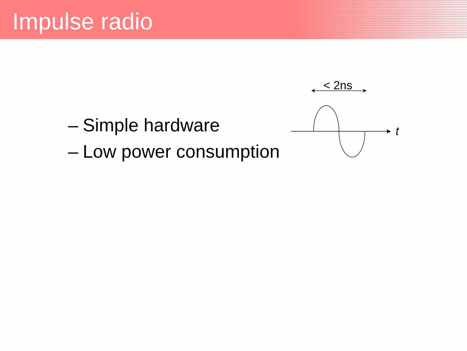
Impulse radio
– Simple hardware– Low power consumption
t
< 2ns

Indoor Multipath Environment
Rx
Rx
Tx
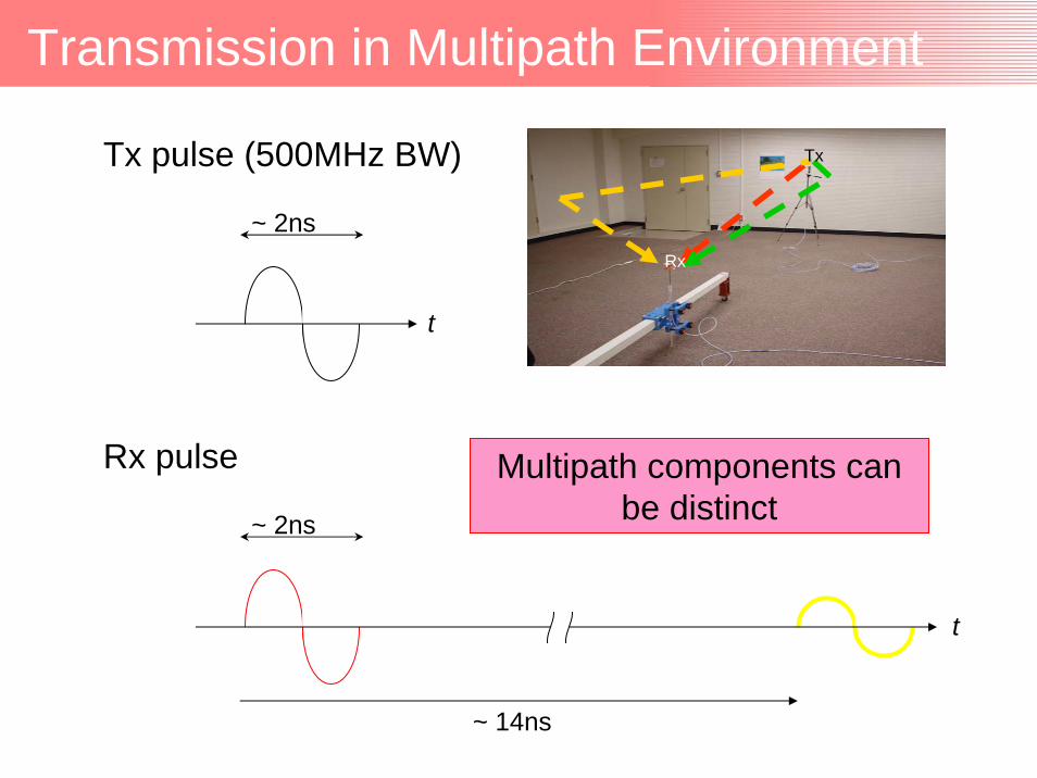
Transmission in Multipath Environment
Rx
Rx
Tx
Rx pulse
t
~ 2ns
Tx pulse (500MHz BW)
t
~ 2ns
~ 14ns
Multipath components can be distinct

Free Space Transfer Function
• Friis’ transmission formula
RxTx
( ) ( ) ( ) ( )RxRxTxTxSpace FreeFriis ,,, ΩHΩH ffdfHfH ⋅=
d
TxΩ RxΩ
f1
∝Normalized by isotropic antenna
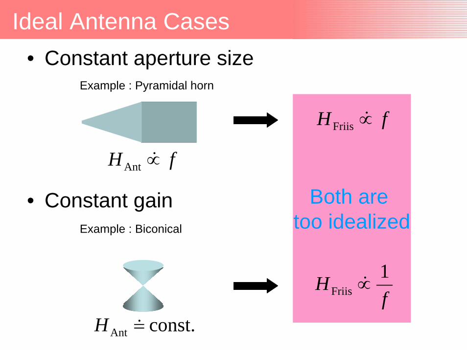
Both are too idealized
• Constant gain
Ideal Antenna Cases
Example : Pyramidal horn
fH ∝Ant
• Constant aperture size
fH ∝Friis
Example : Biconical
const.Ant =Hf
H 1Friis ∝
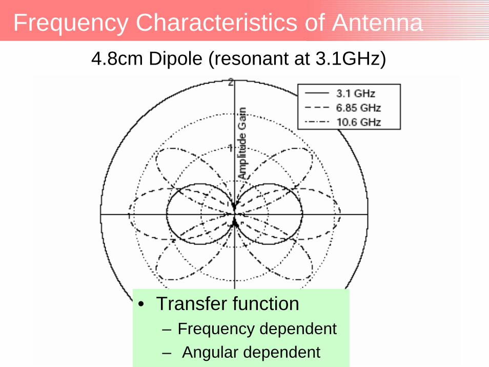
Frequency Characteristics of Antenna4.8cm Dipole (resonant at 3.1GHz)
• Transfer function– Frequency dependent– Angular dependent
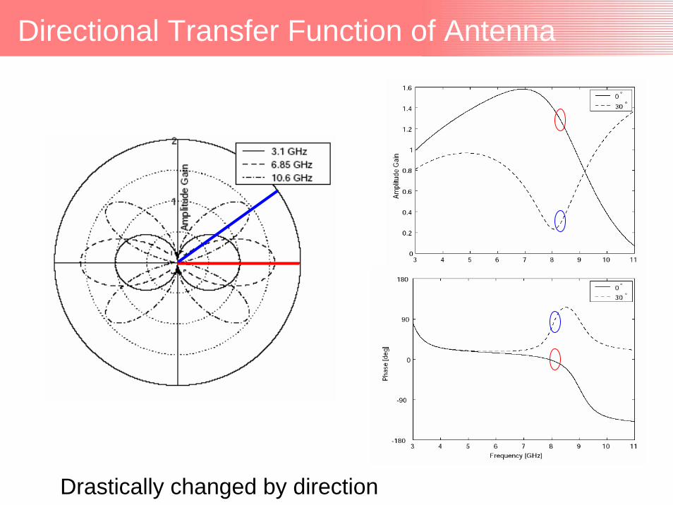
Directional Transfer Function of Antenna
Drastically changed by direction

Directional Impulse Response of Antenna
0.2ns
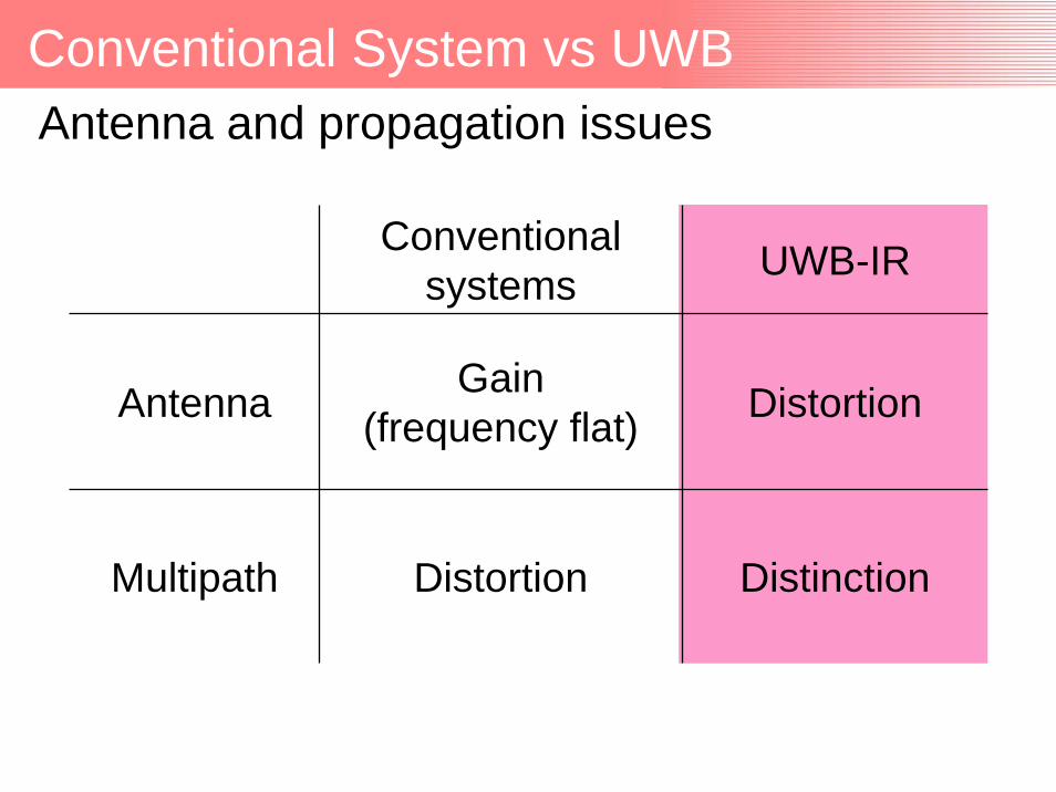
Conventional System vs UWBAntenna and propagation issues
Conventional systems UWB-IR
Antenna Gain(frequency flat) Distortion
Multipath Distortion Distinction

Conventional Channel Model
IEEE 802.15.3a Model
0 20 40 60 80 100 120-1
-0.5
0
0.5
1
1.5Impulse response realizations
Time (nS)
20ns
Channel includes antennas and propagation
Valid only for test antennas (omni) !
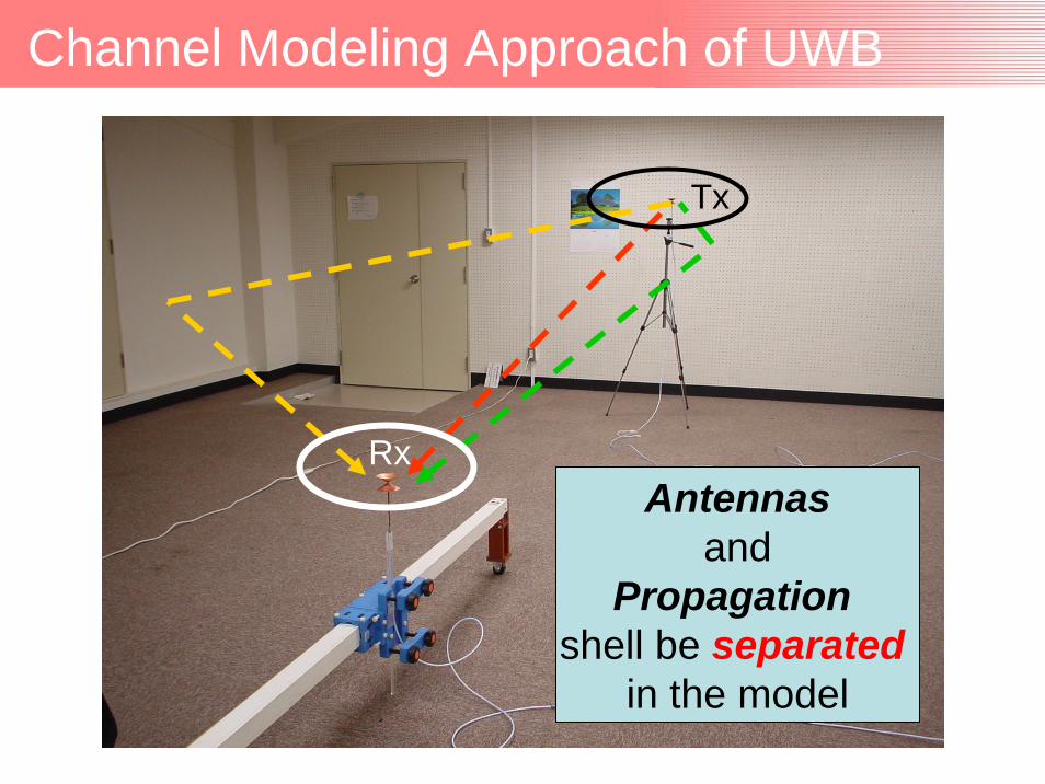
Channel Modeling Approach of UWB
Rx
Rx
Tx
Antennasand
Propagationshell be separated
in the model
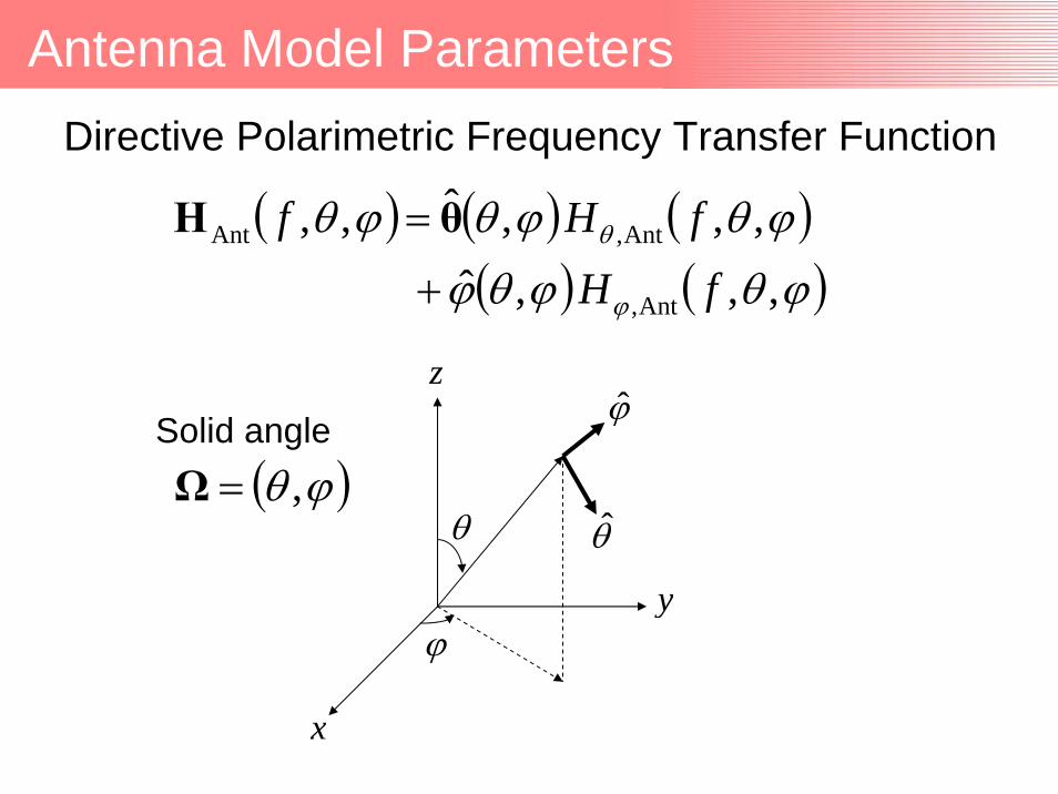
Antenna Model Parameters
( ) ( ) ( )( ) ( )ϕθϕθϕ
ϕθϕθϕθ
ϕ
θ
,,,ˆ,,,ˆ,,
Ant,
Ant,Ant
fHfHf
+
= θH
Directive Polarimetric Frequency Transfer Function
x
y
z
ϕ
θ
ϕ
θ( )ϕθ ,=Ω
Solid angle

How to Get Antenna Model Parameters
• Electromagnetic (EM) wave simulator– MoM (NEC, FEKO, …)– FEM (HFSS, …)– FDTD (XFDTD, …)– …
• Spherical polarimetric measurement– Three antenna method for testing antenna
calibration
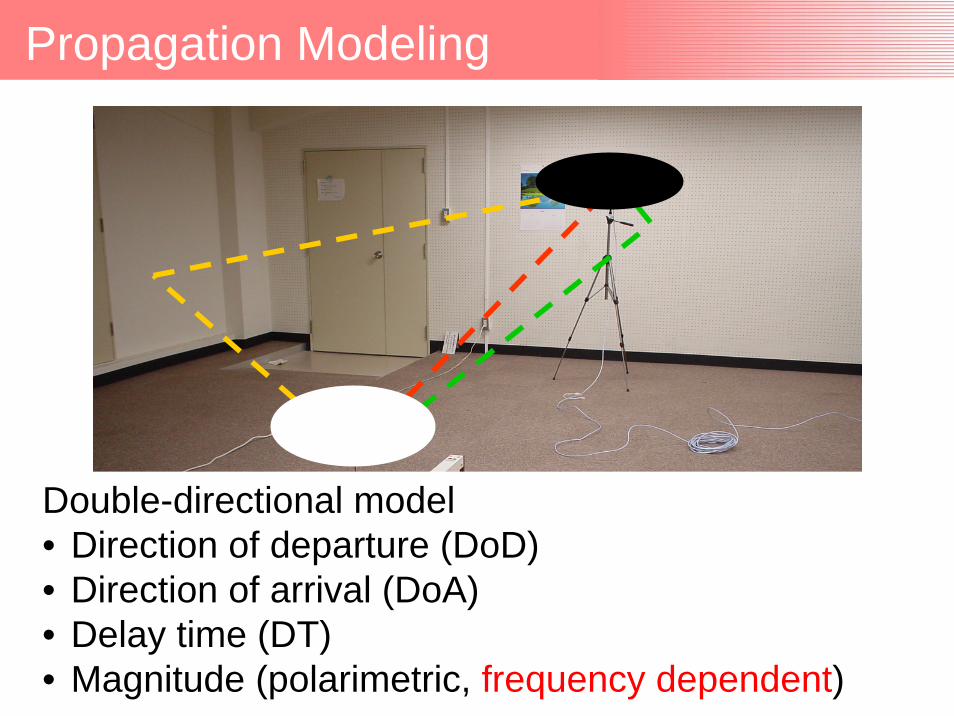
Propagation Modeling
Rx
Rx
Tx
Double-directional model• Direction of departure (DoD)• Direction of arrival (DoA)• Delay time (DT)• Magnitude (polarimetric, frequency dependent)

Double Directional Ray Model
Rx
Rx
Tx
( )
( ) ( ) ( ) ( )∑=
−−−
=L
ll,l,ll ffa
fH
1RxRxTxTx
RxTxMultipath
2jexp
,,
τπδδ ΩΩΩΩ
ΩΩ
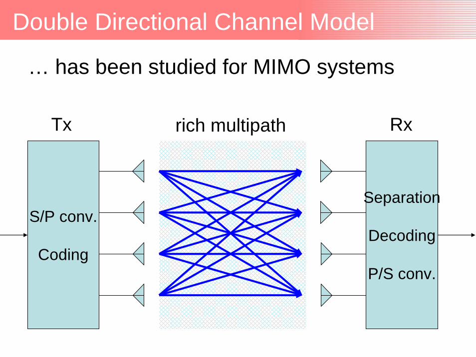
Double Directional Channel Model
… has been studied for MIMO systems
S/P conv.
Coding
Tx
Separation
Decoding
P/S conv.
Rxrich multipath

MIMO Antennas
Design of array antenna is a key issue of MIMO channel capacity.
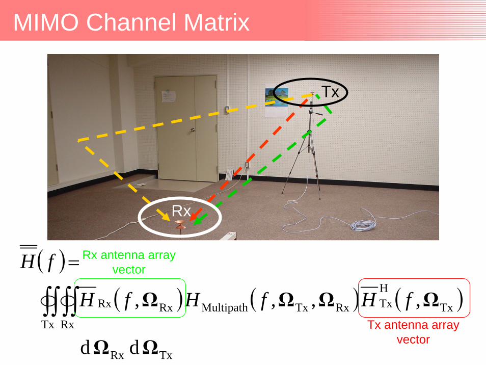
MIMO Channel Matrix
Rx
Rx
Tx
( )( ) ( ) ( )
TxRx
Tx RxTx
HTxRxTxMultipathRxRx
dd
,,,,
ΩΩ
ΩΩΩΩ∫∫ ∫∫=
fHfHfH
fH
Tx antenna arrayvector
Rx antenna arrayvector

MIMO vs UWBAntenna and propagation issues
MIMO UWB-IR
Antenna Array configuration
Frequency distortion
Multipath Double directional
Magnitude Frequency flat Frequency dispersive
Propagation modeling approaches are the same.
Two different aspects of propagation model
• Transmission system design– Stochastic, site generic
• Equipment design and installation– More deterministic, site specific
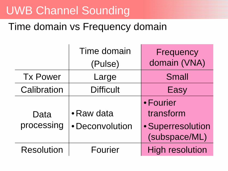
Time domain(Pulse)
Frequency domain (VNA)
Tx Power Large SmallCalibration Difficult Easy
Data processing
• Raw data• Deconvolution
• Fourier transform
• Superresolution(subspace/ML)
Resolution Fourier High resolution
UWB Channel SoundingTime domain vs Frequency domain

UWB Channel SoundingDirective antenna vs Array antenna
Directive antenna
Tx Power Small
Sync. Timing
Data processing
• Raw data• Deconvolution
Resolution Fourier
Array antenna
LargeTiming and
phase• Fourier transform
• Superresolution(subspace/ML)High resolution
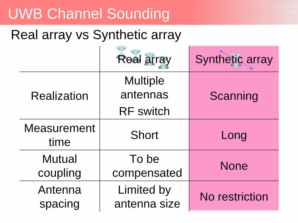
UWB Channel SoundingReal array vs Synthetic array
Real array Synthetic array
RealizationMultiple
antennasRF switch
Scanning
Measurement time Short Long
Mutual coupling
To be compensated None
Antenna spacing
Limited by antenna size No restriction
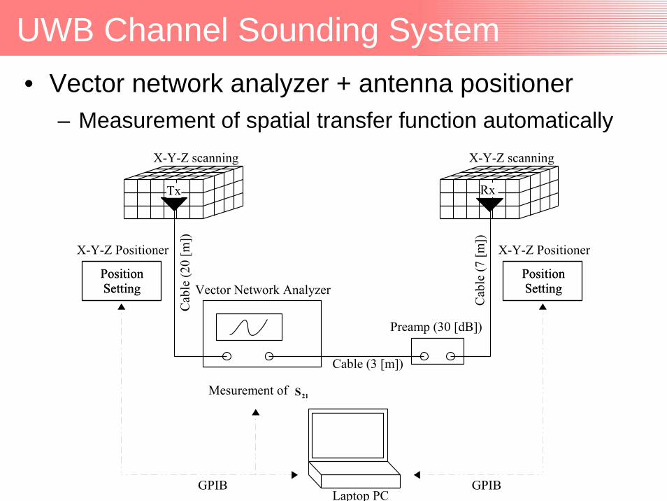
UWB Channel Sounding System • Vector network analyzer + antenna positioner
– Measurement of spatial transfer function automatically

UWB Channel Sounding System
• Pros and Cons– Short range ~ low power handling
• Output power• Cable loss
– Antenna scanning• Static environment• No array calibration
• Architecture– Frequency domain– Synthetic array
– VNA– XY positioner
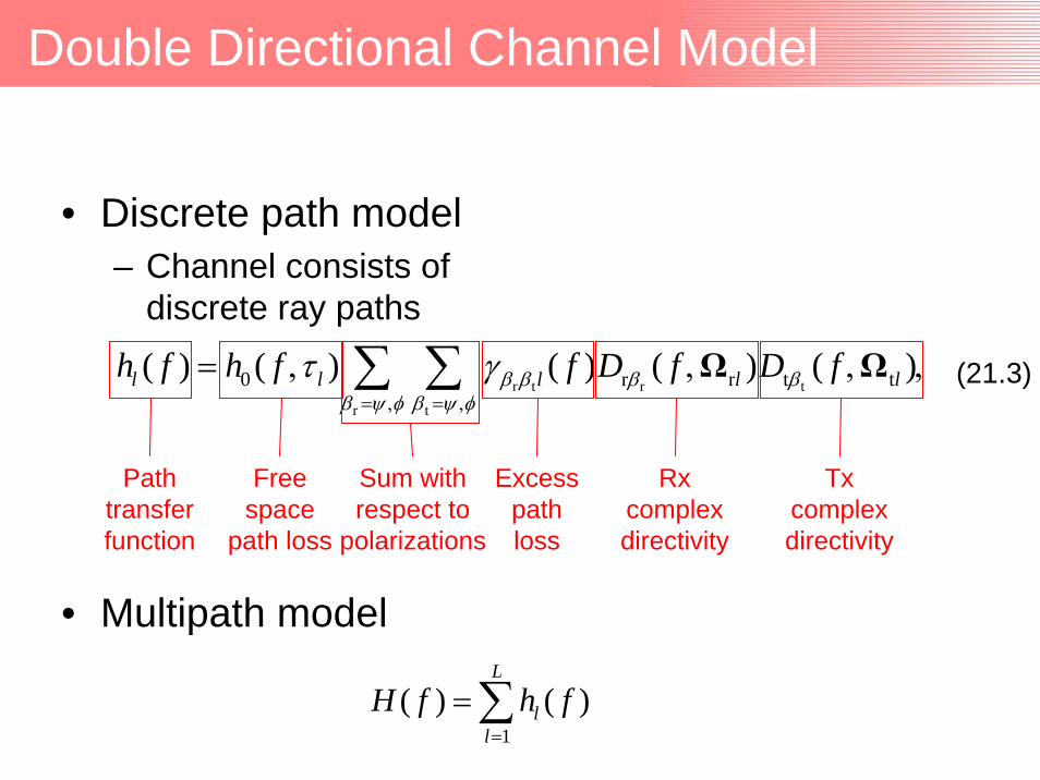
Double Directional Channel Model
• Discrete path model– Channel consists of
discrete ray paths
• Multipath model
r t r t
r t
0 r r t( ) ( ) ( ) ( ) ( )l l l lh f h f f D f D fβ β β ββ ψ φ β ψ φ
τ γ= , = ,
= , , ,t l ,∑ ∑ Ω Ω
Pathtransferfunction
Freespace
path loss
Sum withrespect to
polarizations
Excesspathloss
Rxcomplexdirectivity
Txcomplexdirectivity
1( ) ( )
L
ll
H f h f=
= ∑
(21.3)

Model of Synthetic Array
• Complex gain changes due to position
r r rr r r rˆ ˆ ˆm m m mrx y z= + +r x y z ,
r r rr r r r r2( ) ( ) exp j ˆm m
fD f D fcβ βπ⎛ ⎞, = , ⋅⎜ ⎟
⎝ ⎠Ω Ω r ω
r r r r r rˆ ˆ ˆcos cos cos sin sinˆ
.
ψ φ ψ φ ψ= + + .x y zωPosition vector
Propagation vectorDOA or DOD
x
y
z
φψ
(21.6)
(21.5)
(21.7)

Subband Model
• γ can not be considered as constant over UWB bandwidth.– Piecewise constant
r t r t
r t
0 r r t( ) ( ) ( ) ( ) ( )l l l lh f h f f D f D fβ β β ββ ψ φ β ψ φ
τ γ= , = ,
= , , , ,t l∑ ∑ Ω Ω
f
(21.9)

Spherical Wave Model
• For short range paths, plane wave approximation is not appropriate.– Spherical wave model
Scattering center
Coordinates origin
Spherical wavefront
Rrl
ωrl Direction of propagation can notbe treated as constant.

Spherical Wave Model at Rx Array
t r
r t
0 r r t t
tr r r t
( ) ( ) ( ) ( ) ( )
2 2exp j exp j ˆ
lm m l l l l
ll m l m
h f h f f D f D f
f fRc c
τ γ
π π⎡ ⎤⎛ ⎞⎢ ⎥⎜ ⎟⎢ ⎥⎜ ⎟⎝ ⎠⎢ ⎥⎣ ⎦
= , , ,
⎛ ⎞− − − ⋅⎜ ⎟⎝ ⎠
Ω Ω
R r r ω .
Scattering center
Coordinates origin
Spherical wavefront
Rrl
ωrl
(21.9)
Phase delay correction wrt origin

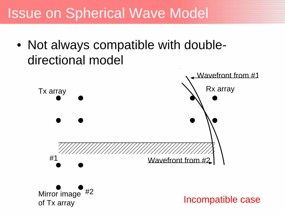
Issue on Spherical Wave Model
• Not always compatible with double-directional model
Rx array
Scattering center seen from Rx
Ray path
Tx array
Wavefront at Tx
Wavefront at Rx
Scattering center seen from Tx
Compatible case
Mirror image of Tx array
Rx arrayTx array
#1
#2
Wavefront from #1
Wavefront from #2
Issue on Spherical Wave Model
• Not always compatible with double-directional model
Incompatible case

Issue on Spherical Wave Model
• SIMO and MISO (single-directional) processing
• Matching by using ray-tracing– Accurate time delay due to UWB
τ1
τ2
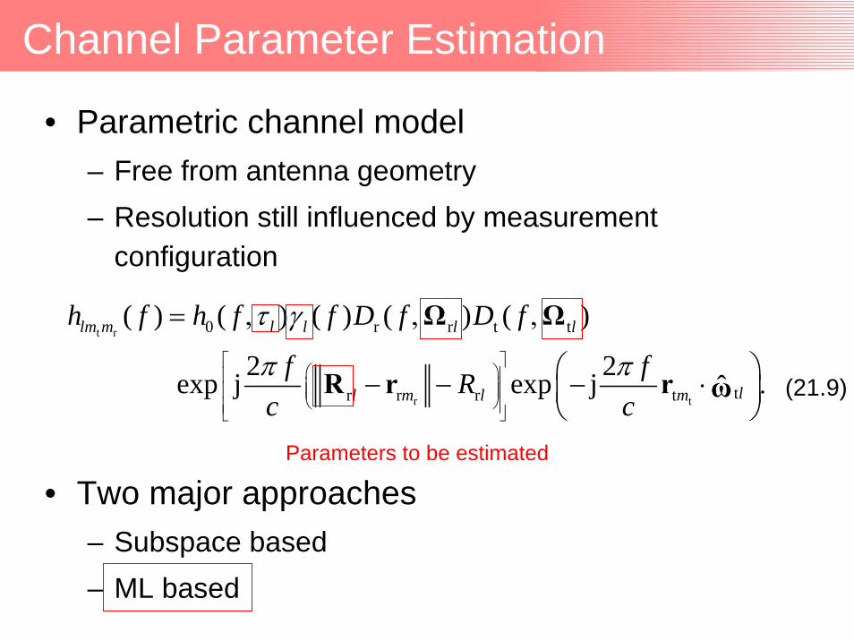
• Parametric channel model– Free from antenna geometry– Resolution still influenced by measurement
configuration
• Two major approaches– Subspace based– ML based
Channel Parameter Estimation
t r
r t
0 r r t t
tr r r t
( ) ( ) ( ) ( ) ( )
2 2exp j exp j ˆ
lm m l l l l
ll m l m
h f h f f D f D f
f fRc c
τ γ
π π⎡ ⎤⎛ ⎞⎢ ⎥⎜ ⎟⎢ ⎥⎜ ⎟⎝ ⎠⎢ ⎥⎣ ⎦
= , , ,
⎛ ⎞− − − ⋅ .⎜ ⎟⎝ ⎠
Ω Ω
R r r ω (21.9)
Parameters to be estimated

Parametric Channel Model
• Measured data contaminated by Gaussian noise
• Parameters to be estimated r r1
Ili l l l ll i
Rγ ψ φ τ⎧ ⎫⎪ ⎪⎨ ⎬
=⎪ ⎪⎩ ⎭= , , , , ,μ
1
L
ll=
= .μ μ∪
r r rm k m k m ky H n= + , (21.11)
r
2var( )m kn σ=
(21.12)
(21.13)
DOA or DOD
x
y
z
φψ
τ1
τ2
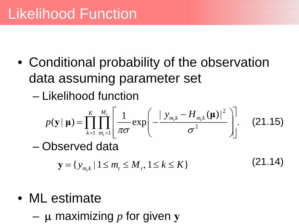
Likelihood Function
• Conditional probability of the observation data assuming parameter set– Likelihood function
– Observed data
• ML estimate– μ maximizing p for given y
r r r 1 1 m ky m M k K= | ≤ ≤ , ≤ ≤y
rr r
r
2
21 1
( )1( ) expMK
m k m k
k m
y Hp
πσ σ= =
⎡ ⎤⎛ ⎞| − || = − .⎢ ⎥⎜ ⎟⎜ ⎟⎢ ⎥⎝ ⎠⎣ ⎦
∏∏μ
y μ (21.15)
(21.14)
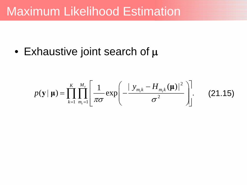
Maximum Likelihood Estimation
• Exhaustive joint search of μ
rr r
r
2
21 1
( )1( ) expMK
m k m k
k m
y Hp
πσ σ= =
⎡ ⎤⎛ ⎞| − || = − .⎢ ⎥⎜ ⎟⎜ ⎟⎢ ⎥⎝ ⎠⎣ ⎦
∏∏μ
y μ (21.15)

Expectation Maximization (EM) Algorithm
• Estimate of “complete data” x from “incomplete data” y (E-step)
• ML applied to “complete data” (M-step)
( )l l lb= + − .x h y H (21.17)
2arg max ( ) arg min ( )l
l l l lp | = − .x μ x h μμμ (21.19)
Least square problemto be solved by matched filtering
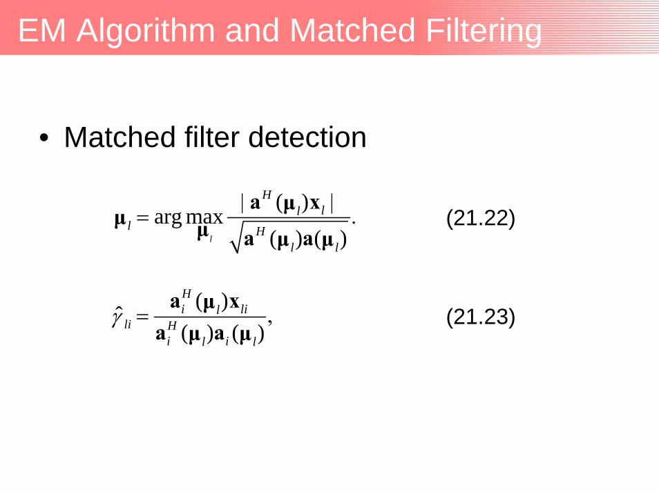
EM Algorithm and Matched Filtering
• Matched filter detection
( )arg max
( ) ( )l
Hll
l Hl l
| |= .
a xμμ μ a aμ μ
(21.22)
( )ˆ( ) ( )
Hi lil
li Hi il l
γ = ,a xμa aμ μ
(21.23)
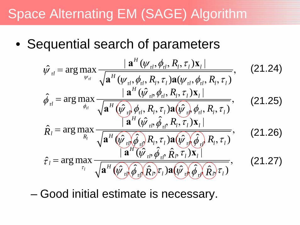
• Sequential search of parameters
– Good initial estimate is necessary.
Space Alternating EM (SAGE) Algorithm
r
r rr
r r r r
( )ˆ arg max( ) ( )l
Hl l l l l
l Hl l l l l l l l
RR Rψ
ψ φ τψ
ψ φ τ ψ φ τ
| , , , |= ,
, , , , , ,
a xa a
r
rrr
r rr r
ˆ( )ˆ arg maxˆ ˆ( ) ( )l
Hl l l ll
l Hl l l l l ll l
R
R Rφ
φ τψφ
φ τ φ τψ ψ
| , , , |= ,
, , , , , ,
a x
a ar r
r rr r
ˆˆ( )ˆ arg max
ˆ ˆˆ ˆ( ) ( )l
Hl l ll l
l HRl l l ll ll l
RR
R R
τψ φτ τψ ψφ φ
| , , , |= ,
, , , , , ,
a x
a ar r
r rr r
ˆˆ ˆ( )arg maxˆ
ˆ ˆˆ ˆ ˆ ˆ( ) ( )l
Hl ll ll
l Hl ll l l ll l
R
R Rτ
τψ φτ
τ τψ ψφ φ
| , , , |= ,
, , , , , ,
a x
a a
(21.24)
(21.25)
(21.26)
(21.27)

Successive Cancellation Approach
l = 1
Rough global search of l-th path
Fine local search of l-th pathby SAGE
Subtraction of l-th path from observation
Convergence? end
l = l + 1No model order estimationIn advance.

Tx (1)
Rx
Rx
Tx
• Measurement site: an empty room
X-Y scanner
Experiment in an Indoor Environment (1)

• Floor plan of the room
Experiment in an Indoor Environment (2)

• Estimated parameters : DoA (Az, El), DT• Measured data :
– Spatially 10 by 10 points at Rx– 801 points frequency sweeping from 3.1 to 10.6
[GHz] (sweeping interval: 10 [MHz])• Antennas : Biconical antennas for Tx and Rx• Calibration : Function of VNA, back-to-back• IF Bandwidth of VNA : 100 [Hz]• Wave polarization : Vertical - Vertical• Bandwidth of each subband : 800 [MHz]
Experiment in an Indoor Environment (3)
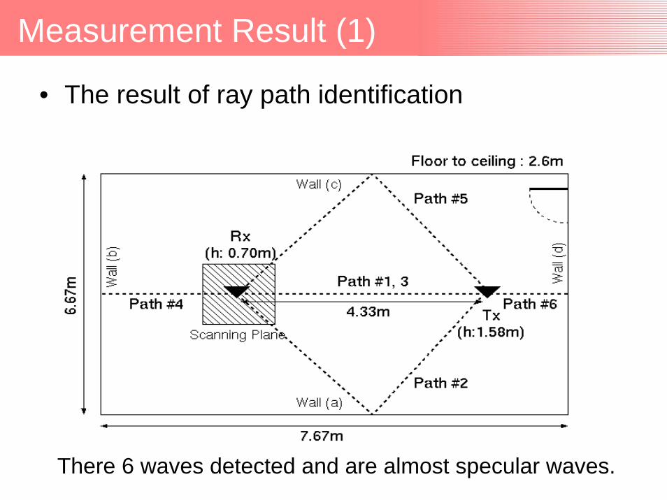
• The result of ray path identification
There 6 waves detected and are almost specular waves.
Measurement Result (1)
Tx (1)
Rx
Rx
Tx
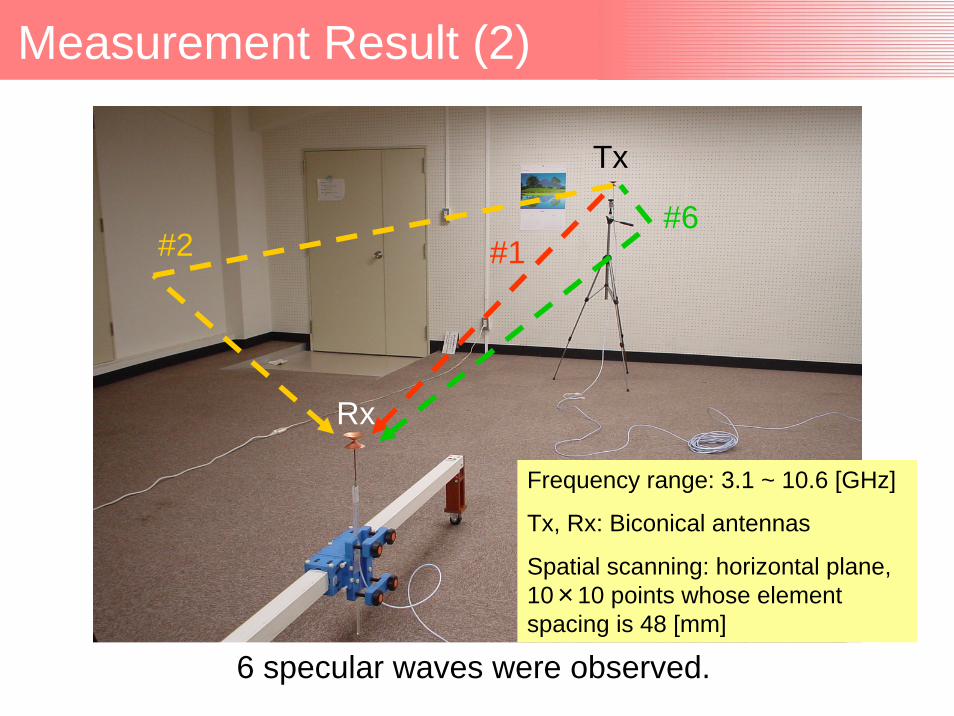
Measurement Result (2)
6 specular waves were observed.
#1#6
#2
Frequency range: 3.1 ~ 10.6 [GHz]
Tx, Rx: Biconical antennas
Spatial scanning: horizontal plane, 10×10 points whose element spacing is 48 [mm]

Tx (1)
Rx
Rx
Tx
#4 is a reflection from the back of Rx
#1
#3
#5
Rx
Tx#4
Tx
Rx#1
Measurement Result (3)

• Extracted spectrum of direct wave
– Transfer functions of antennas are already deconvolved.– The phase component is the deviation from free space
phase rotation (ideally flat).
Measurement Result (4)
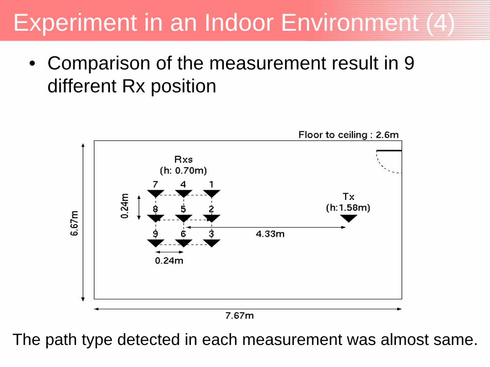
• Comparison of the measurement result in 9 different Rx position
The path type detected in each measurement was almost same.
Experiment in an Indoor Environment (4)
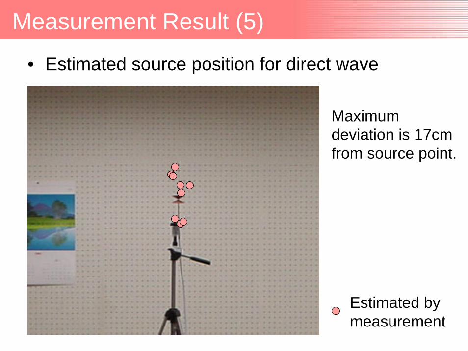
• Estimated source position for direct wave
Estimated by measurement
Maximum deviation is 17cm from source point.
Measurement Result (5)
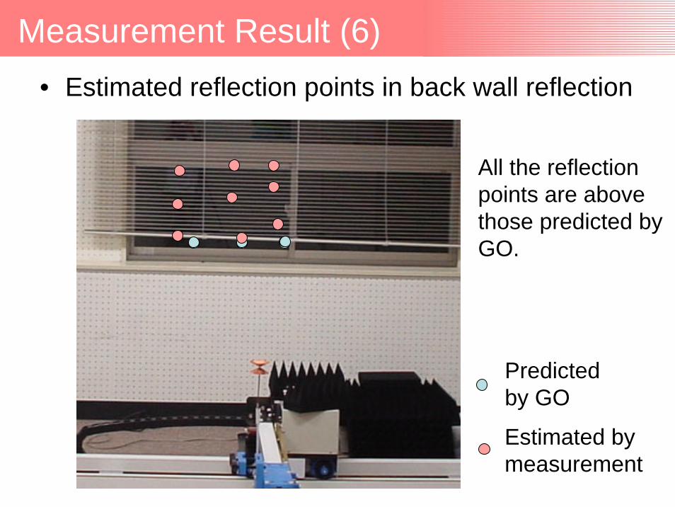
• Estimated reflection points in back wall reflection
Estimated by measurement
Predicted by GO
All the reflection points are above those predicted by GO.
Measurement Result (6)
• Some problems have been appeared.– 2 ~ 4 spurious waves detected during the
estimation of 6 waves– Residual components after removing dominant
paths– Signal model error (plane or spherical)– Estimation error based on inherent resolution of
the algorithm implementation– Many distributed source points (diffuse
scattering)
Discussion
Further investigation in simple environment

Performance Evaluation in Anechoic Chamber
VNA
PC
Synthesized URA
X-Y Scanner
GPIB
Tx2
GPIB
Tx1
3-dB power splitter
Anechoic chamber

Specifications of Experiment
• Frequency : 3.1 ~ 10.6 GHz– 0.13 ns Fourier resolution
• Antenna scanning plane : 432 mm square in horizontal plane– 10 deg Fourier resolution– 48 mm element spacing
(less than half wavelength @ 3.1 GHz)
• Wideband monopole antennas were used– Variation of group delay < 0.1 ns within the
considered bandwidth
• SNR at receiver: About 25 dB

Aim of Anechoic Chamber Test
• Evaluation of spatio-temporal resolution
– Separation and detection of two waves that
• Spatially 10 deg different and same DT
• Temporally 0.67 ns ( = 20 cm ) different and same
DoA

Setup of Experiment
Tx
Rx
X-Y scanner

Spatial Resolution Test (1)
Tx1 Tx2
10 deg
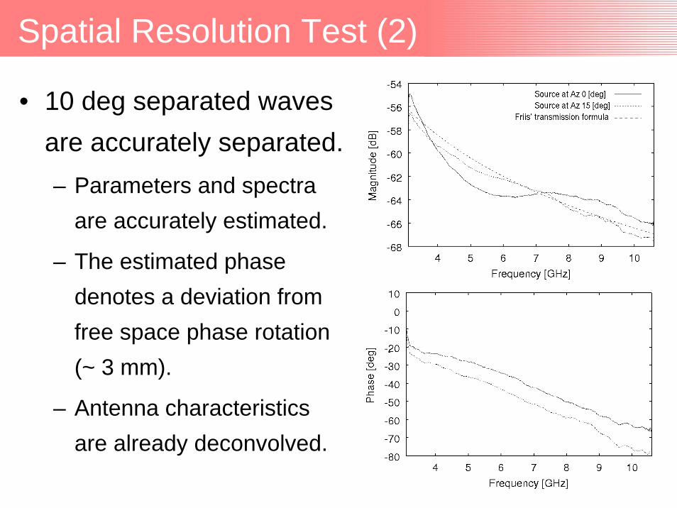
Spatial Resolution Test (2)
• 10 deg separated waves are accurately separated.– Parameters and spectra
are accurately estimated.
– The estimated phase denotes a deviation from free space phase rotation (~ 3 mm).
– Antenna characteristics are already deconvolved.
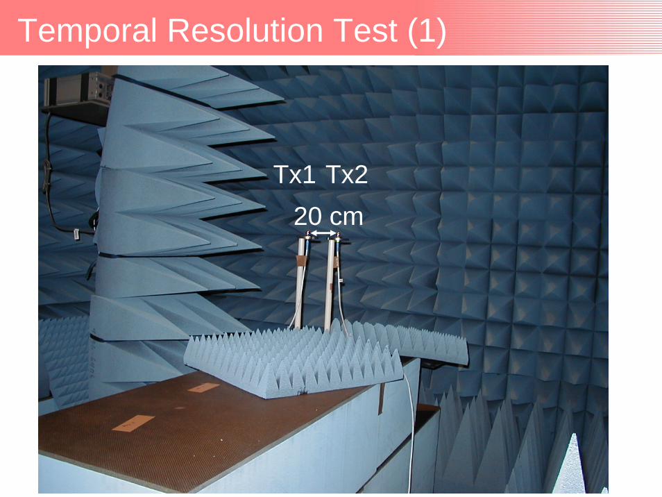
Temporal Resolution Test (1)
Tx1 Tx220 cm
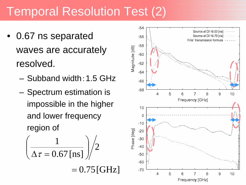
Temporal Resolution Test (2)
• 0.67 ns separated waves are accurately resolved.– Subband width:1.5 GHz
– Spectrum estimation is impossible in the higher and lower frequency region of
2[ns] 67.0
1⎟⎟⎠
⎞⎜⎜⎝
⎛=Δτ
[GHz] 75.0=

Subband Processing (1)• … relieves a bias of parameter estimation due to
amplitude and phase fluctuation within the band • Tradeoff between the resolution and accuracy of
parameter estimation: some optimization is needed !!
Log-
likel
ihoo
d
Frequency
π 0
00
Cancel ?
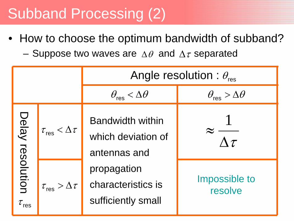
Subband Processing (2)• How to choose the optimum bandwidth of subband?
– Suppose two waves are and separated
Angle resolution :
Delay resolution
Bandwidth within which deviation of antennas and propagation characteristics is sufficiently small
Impossible to resolve
θΔ τΔ
θθ Δ<res
ττ Δ<res
τΔ≈
1
resθ
θθ Δ>res
resτττ Δ>res
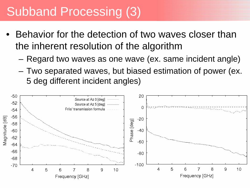
Subband Processing (3)
• Behavior for the detection of two waves closer than the inherent resolution of the algorithm– Regard two waves as one wave (ex. same incident angle)– Two separated waves, but biased estimation of power (ex.
5 deg different incident angles)

Deconvolution of Antenna Patterns
• Deconvolution of antennas
– Construction of channel models independent
of antenna type and antenna configuration
– Deconvolution is post-processing (from the
estimated spectrum by SAGE)
• Simple implementation rather than the
deconvolution during the search

Spherical vs Plane Wave Models (1)
• How these models affect for the accurate estimation?– Spurious (ghost path) and detection of weak paths – Empirical evaluation of model accuracy
Plane wave incidence (far field incidence)
Spherical wave incidence (radiation from point source)

Spherical vs Plane Wave Models (2)• Detection of 20 dB different two waves
– Is a weaker source correctly detected?
#2 = 15 deg20 dB weaker #1 = 0 deg
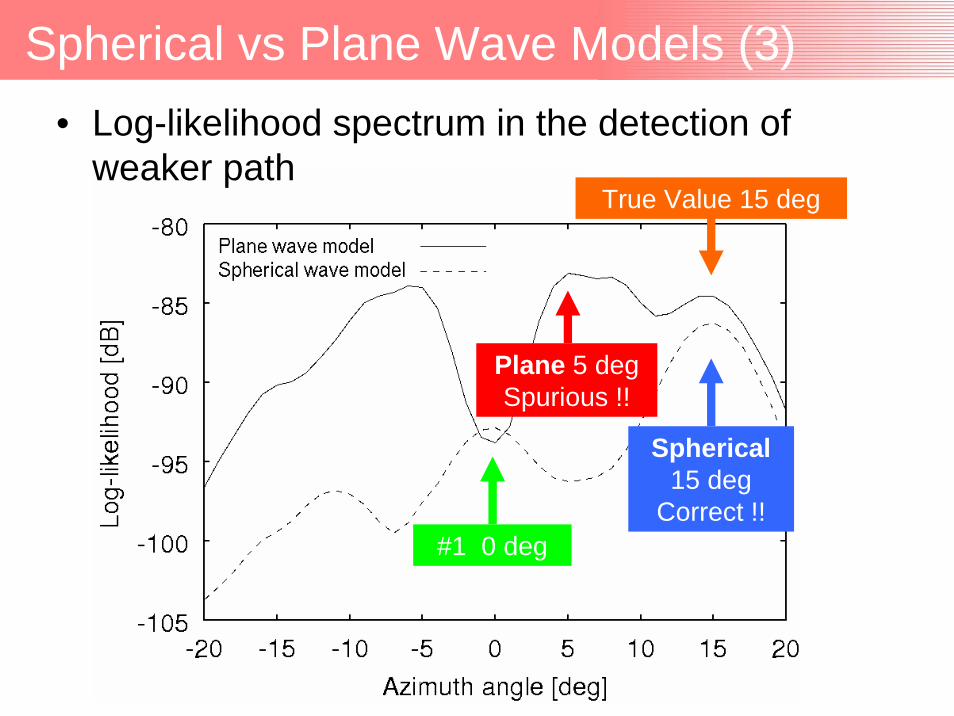
Spherical vs Plane Wave Models (3)
Spherical 15 deg
Correct !!
Plane 5 deg Spurious !!
True Value 15 deg
#1 0 deg
• Log-likelihood spectrum in the detection of weaker path
Summary of Evaluation Works (1)
• Evaluation of the proposed UWB channel
sounding system in an anechoic chamber
– Resolved spatially 10 deg, temporally 0.67 ns
separated waves
– Spectrum estimation is partly impossible in the highest
and lowest frequency regions of .
– The algorithm treats two waves closer than inherent
resolution as one wave, or results in biased power
estimation even if they are separated.
τΔ21

Summary of Evaluation Works (2)
• For reliable UWB channel estimation with SAGE algorithm– An optimum way to choose the bandwidth of subband
– The number of waves estimation is done by SIC- type procedure
• Deconvolution of antennas effects from the results of SAGE– For channel models independent of antennas
Summary of Evaluation Works (3)
• Spherical incident wave model is more robust than plane wave incident model– Spurious reduction is expected
– Effective in the detection of weaker path

Indoor Double Directional Measurement (1)
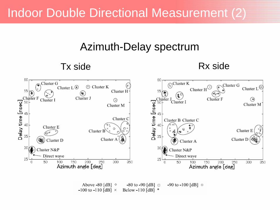
Indoor Double Directional Measurement (2)
Tx side
Azimuth-Delay spectrum
Rx side
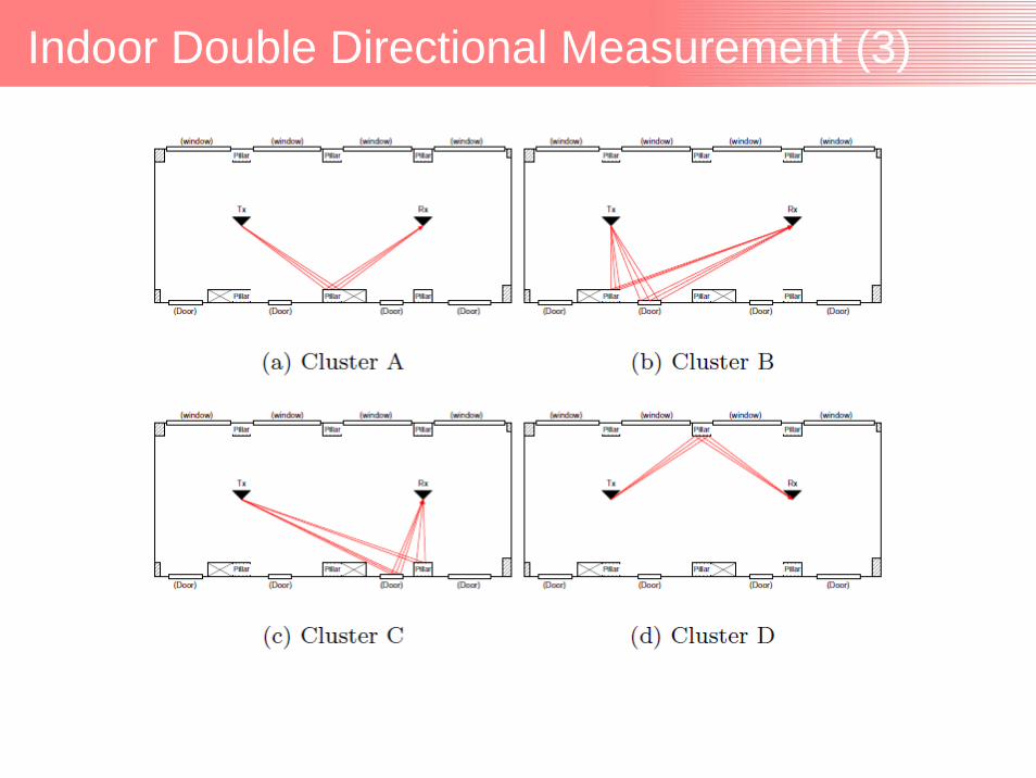
Indoor Double Directional Measurement (3)

Indoor Double Directional Measurement (4)
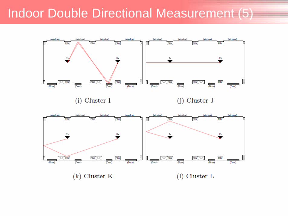
Indoor Double Directional Measurement (5)
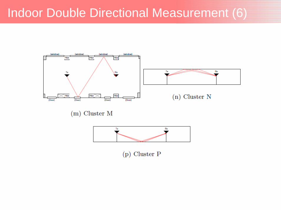
Indoor Double Directional Measurement (6)
Summary
• Background and motivation of double directional sounding
• Antennas and propagation in UWB• UWB double directional channel sounding
system• Parametric multipath modeling for UWB• ML-based parameter estimation• Examples

References
• Jun-ichi Takada, Katsuyuki Haneda, and Hiroaki Tsuchiya, "Joint DOA/DOD/DTOA estimation system for UWB double directional channel modeling," to be published in S. Chandran (eds), "Advances in Direction of Arrival Estimation," to be published from ArtechHouse, Norwood, MA, USA.
• Katsuyuki Haneda, Jun-ichi Takada, and Takehiko Kobayashi, "Experimental Evaluation of a SAGE Algorithm for Ultra Wideband Channel Sounding in an Anechoic Chamber," joint UWBST & IWUWBS 2004 International Workshop on Ultra Wideband Systems Joint with Conference on Ultra Wideband Systems and Technologies (Joint UWBST & IWUWBS 2004), May 2004 (Kyoto, Japan).
• Hiroaki Tsuchiya, Katsuyuki Haneda, and Jun-ichi Takada, "UWB Indoor Double-Directional Channel Sounding for Understanding the Microscopic Propagation Mechanisms," 7th International Symposium on Wireless Personal Multimedia Communications (WPMC 2004), pp. 95-99, Sept. 2004 (Abano Terme, Italy).