Utilizing maximum power point trackers in parallel to maximize the

Calhoun: The NPS Institutional Archive

DSpace Repository

Theses and Dissertations 1. Thesis and Dissertation Collection, all items

2012-12

Utilizing maximum power point trackers in

parallel to maximize the power output of a

solar (photovoltaic) array

Stephenson, Christopher A.

Monterey, California. Naval Postgraduate School

http://hdl.handle.net/10945/27907

Downloaded from NPS Archive: Calhoun

NAVAL

POSTGRADUATE SCHOOL

MONTEREY, CALIFORNIA

THESIS

Approved for public release; distribution is unlimited

UTILIZING MAXIMUM POWER POINT TRACKERS IN PARALLEL TO MAXIMIZE THE POWER OUTPUT OF A

SOLAR (PHOTOVOLTAIC) ARRAY

by

Christopher Alan Stephenson

December 2012

Thesis Advisor: Sherif Michael Second Reader: Robert Ashton

THIS PAGE INTENTIONALLY LEFT BLANK

i

REPORT DOCUMENTATION PAGE Form Approved OMB No. 0704–0188Public reporting burden for this collection of information is estimated to average 1 hour per response, including the time for reviewing instruction, searching existing data sources, gathering and maintaining the data needed, and completing and reviewing the collection of information. Send comments regarding this burden estimate or any other aspect of this collection of information, including suggestions for reducing this burden, to Washington headquarters Services, Directorate for Information Operations and Reports, 1215 Jefferson Davis Highway, Suite 1204, Arlington, VA 22202–4302, and to the Office of Management and Budget, Paperwork Reduction Project (0704–0188) Washington DC 20503. 1. AGENCY USE ONLY (Leave blank)

2. REPORT DATE December 2012

3. REPORT TYPE AND DATES COVERED Master’s Thesis

4. TITLE AND SUBTITLE Utilizing Maximum Power Point Trackers in Parallel to Maximize the Power Output of a Solar (Photovoltaic) Array

5. FUNDING NUMBERS

6. AUTHOR(S) Christopher A. Stephenson 7. PERFORMING ORGANIZATION NAME(S) AND ADDRESS(ES)

Naval Postgraduate School Monterey, CA 93943–5000

8. PERFORMING ORGANIZATION REPORT NUMBER

9. SPONSORING /MONITORING AGENCY NAME(S) AND ADDRESS(ES)

N/A

10. SPONSORING/MONITORING AGENCY REPORT NUMBER

11. SUPPLEMENTARY NOTES The views expressed in this thesis are those of the author and do not reflect the official policy or position of the Department of Defense or the U.S. Government. IRB Protocol number: N/A. 12a. DISTRIBUTION / AVAILABILITY STATEMENT Approved for public release; distribution is unlimited

12b. DISTRIBUTION CODE

13. ABSTRACT (maximum 200 words)

It is common when optimizing a photovoltaic (PV) system to use a maximum power point tracker (MPPT) to increase the power output of the solar array. Currently, most military applications that utilize solar energy omit or use only a single MPPT per PV system. The focus of this research was to quantify the expected benefits of using multiple MPPTs within a PV system based on current technologies and to summarize what may be possible in the near future. In this thesis, the advertised 5–8% gains in efficiency claimed by manufacturers of the multiple MPPT approach were tested and a set of generalized recommendations concerning which applications may benefit from this distributed approach, and which ones may not were sought. The primary benefit of utilizing multiple MPPTs is the concept that independently operating panels within a solar array could increase the overall reliability and resiliency of the entire PV system and potentially allow for solar applications to be used in particularly harsh and dynamic environments with increased confidence. Additionally, using multiple, smaller MPPTs could decrease the overall array dimensions that would save space, reduce weight, and lower costs.

14. SUBJECT TERMS Solar Efficiency, Maximum Power Point Tracker, Micro-inverter, Micro-converter, Power Optimizer, Distributed Solar Array

15. NUMBER OF PAGES

137 16. PRICE CODE

17. SECURITY CLASSIFICATION OF REPORT

Unclassified

18. SECURITY CLASSIFICATION OF THIS PAGE

Unclassified

19. SECURITY CLASSIFICATION OF ABSTRACT

Unclassified

20. LIMITATION OF ABSTRACT

UU NSN 7540–01–280–5500 Standard Form 298 (Rev. 2–89) Prescribed by ANSI Std. 239–18

ii


iii

Approved for public release; distribution is unlimited

UTILIZING MAXIMUM POWER POINT TRACKERS IN PARALLEL TO MAXIMIZE THE POWER OUTPUT OF A SOLAR (PHOTOVOLTAIC) ARRAY

Christopher A. Stephenson Captain, United States Marine Corps

B.A., United States Naval Academy, 2003

Submitted in partial fulfillment of the requirements for the degree of

MASTER OF SCIENCE IN ELECTRICAL ENGINEERING

from the

NAVAL POSTGRADUATE SCHOOL December 2012

Author: Christopher A. Stephenson

Approved by: Sherif Michael Thesis Advisor

Robert Ashton Second Reader

R. Clark Robertson Chair, Department of Electrical and Computer Engineering

iv


v

ABSTRACT

It is common when optimizing a photovoltaic (PV) system to

use a maximum power point tracker (MPPT) to increase the

power output of the solar array. Currently, most military

applications that utilize solar energy omit or use only a

single MPPT per PV system. The focus of this research was

to quantify the expected benefits of using multiple MPPTs

within a PV system based on current technologies and to

summarize what may be possible in the near future. In this

thesis, the advertised 5–8% gains in efficiency claimed by

manufacturers of the multiple MPPT approach were tested and

a set of generalized recommendations concerning which

applications may benefit from this distributed approach,

and which ones may not were sought. The primary benefit of

utilizing multiple MPPTs is the concept that independently

operating panels within a solar array could increase the

overall reliability and resiliency of the entire PV system

and potentially allow for solar applications to be used in

particularly harsh and dynamic environments with increased

confidence. Additionally, using multiple, smaller MPPTs

could decrease the overall array dimensions that would save

space, reduce weight, and lower costs.

vi


vii

TABLE OF CONTENTS

I. INTRODUCTION ............................................1 A. BACKGROUND .........................................1 B. OBJECTIVES .........................................2 C. SCOPE, ORGANIZATION, AND METHODOLOGY ...............2

1. Scope and Organization ........................2 2. Methodology ...................................3 3. Related Work ..................................3

D. EXPECTED BENEFITS ..................................4

II. SOLAR CELL BASICS .......................................7 A. HOW A BASIC SOLAR CELL IS CREATED ..................7

1. The p-Type n-Type (p-n) Junction ..............7 2. Forward Bias ..................................8 3. Solar Radiation to Electric Energy ...........10

B. SOLAR CELL PARAMETERS .............................11 1. Open Circuit Voltage .........................11 2. Short Circuit Current ........................12 3. Efficiency and Fill Factor ...................13

C. SOLAR CELL EFFICIENCY VARIABLES ...................14 1. Irradiance ...................................15 2. Recombination ................................15 3. Temperature ..................................16 4. Reflection ...................................16 5. Electrical Resistance ........................16 6. Material Defects and Self-shading ............17

III. MAXIMUM POWER POINT TRACKERS ...........................19 A. MPPT DESIGN PRINCIPLES ............................19 B. ANALYSIS OF TRACKING ALGORITHMS ...................22

1. Perturb and Observe ..........................22 2. Constant Voltage and Constant Current ........25 3. Pilot Cell ...................................28 4. Incremental Conductance ......................28 5. Model-based Algorithm ........................31 6. Parasitic Capacitance ........................32 7. MPPT Algorithm Performance ...................34

C. ANALOG VERSUS DIGITAL MPPT DESIGN .................36 1. Digital Design ...............................36 2. Analog Design ................................40

a. Analog Perturb and Observe of the Load Current .................................41

b. TEODI .....................................43 D. MPPT CONVERTER TECHNOLOGY .........................46

viii

1. Inductively Fed, Switch-mode DC-DC Converters ...................................46

2. MPPT Converter Design ........................49

IV. POTENTIAL APPLICATIONS .................................51 A. INTRODUCTION ........................................51 B. A CASE FOR MULTIPLE MPPTS ...........................52 C. SPACE APPLICATIONS ..................................57

1. Direct Loading Versus Central Converter Approach .....................................58

2. Micro-converter Approach .....................60 D. MILITARY APPLICATIONS .............................63

1. Tactical Solar Tents and Shelters ............63 2. Unmanned Aerial Vehicles .....................65

V. TEST AND DATA ANALYSIS .................................67 A. INTRODUCTION ........................................67

1. Amprobe Solar 600 Analyzer ...................67 2. Radiant Source Technology (RST) Solar

Simulator ....................................68 3. Fluke 45 Dual Display Multimeter .............69

B. MPPT SELECTION ......................................70 1. STEVAL SPV1020 MPPT with DC-DC Boost

Converter ....................................70 a. STEVAL-ISV009V1 Specifications ..........70 b. ISV009V1 Testing ........................71 c. ISV009V1 Demo Board Test Conclusions ....73

2. Genasun-4 MPPT with DC-DC Buck Converter .....74 a. Genasun-4 Specifications ................75 b. Genasun-4 Testing .......................76 c. Genasun-4 MPPT Test Results .............77

C. SOLAR PANEL SELECTION ...............................78 D. FINAL DESIGN ........................................79 E. DATA ................................................81 F. OBSERVATIONS ........................................84

1. MPPTs Outperform the Direct Loading Approach .84 2. Micro-inverters Versus Central Converter .....84 3. Tracking Accuracy ............................85 4. Bypass Mode ..................................85 5. MPP error during central converter test ......86

VI. CONCLUSIONS ............................................89 A. CONCLUSIONS .........................................90

1. MPPT Versus Direct-Loading ...................90 2. Multiple MPPT Performance ....................91 3. FF Versus MPPT Performance ...................91

B. RECOMMENDATIONS FOR FUTURE WORK .....................92

ix

1. A More Refined Method in Validating the Nultiple MPPT Approach .......................92

2. Design of a “Per Cell” MPPT ..................93 3. Capacitor-Based Converter Technologies .........93

APPENDIX A. STEVAL ISV009V1 SCHEMATIC .......................95

APPENDIX B. AMPROBE SOLAR-600 ANALYSIS EXAMPLE ..............97

APPENDIX C. TEST RESULTS ....................................99

LIST OF REFERENCES .........................................103

INITIAL DISTRIBUTION LIST ..................................107

x


xi

LIST OF FIGURES

Figure 1. A depiction of the p-n junction (After [2])......7 Figure 2. Forward biasing of a p-n Junction (From [2]).....9 Figure 3. The generation of photocurrent in a solar cell

(From [3])......................................11 Figure 4. The p-n junction under open circuit conditions

VOC (From [2]). .................................12 Figure 5. The p-n junction under short circuit current

conditions (From [2])...........................13 Figure 6. A typical I-V curve with MPP depicted (From

[2])............................................14 Figure 7. The operating point of a directly-coupled PV

array and load (From [10])......................20 Figure 8. A PV I-V curve at 40°C for different irradiance

levels (After [10]).............................21 Figure 9. The P-V relationship at different irradiance

levels (From [10])..............................23 Figure 10. An illustration of erratic behavior when the

P&O algorithm is exposed to rapidly increasing irradiance (From [10])..........................24

Figure 11. A flowchart depicting the constant voltage algorithm (From [10])...........................26

Figure 12. VMPP as a percentage of VOC (constant K) as functions of temperature and irradiance (From [10])...........................................27

Figure 13. A flowchart of the incremental conductance algorithm (From [10])...........................31

Figure 14. The circuitry used when implementing the parasitic capacitance algorithm (From [10]).....34

Figure 15. Change of current operating points when the irradiance changes for different adaptive P&O algorithms (From [12])..........................38

Figure 16. A PV System with a load current-based analog MPPT controller (From [13]).....................41

Figure 17. Schematic of a basic analog MPPT controller (After [13])....................................42

Figure 18. Location of TEODI case 2 operating points on a notional P-V curve (From [13])..................44

Figure 19. A typical efficiency curve of an inductively fed, switch-mode DC/DC converter (From [16])....48

Figure 20. The size of an evaluation board containing a 300 watt digital MPPT with boost DC-DC converter.......................................50

xii

Figure 21. An example of a severely obstructed panel. Note the four panels completely unobstructed (From [18])...........................................53

Figure 22. An example of a homogeneous array exposed to similar environmental conditions................56

Figure 23. An image of PANSAT (From [22])..................57 Figure 24. Top view of the PANSAT satellite (From [22])....58 Figure 25. Hypothetical I-V response curve of a PANSAT

satellite wired as a single array...............59 Figure 26. Simulated I-V curve response of a PANSAT

satellite using them micro-inverter approach....61 Figure 27. Simulated P-V curve response of a PANSAT

satellite using the micro-converter approach....62 Figure 28. The Energy Technologies, Inc. Tactical Solar

Tent (From [23])................................64 Figure 29. The AeroVironment Raven RQ-11 UAV

(manufacturer’s image)..........................65 Figure 30. The Amprobe Solar-600 Analyzer (From [24])......68 Figure 31. The RST Solar Simulator (From [25]).............69 Figure 32. The input and output parameters required for

efficiency calculations.........................69 Figure 33. A distributed PV system using multiple MPPTs

(From [26]).....................................70 Figure 34. The actual MPP versus the ISV009V1 MPPT

operating point of the PANSAT array in the RST solar simulator.................................73

Figure 35. Circuit diagram of the Genasun-4 test set-up....75 Figure 36. The Genasun-4 MPPT with DC-DC buck converter

and charge controller...........................76 Figure 37. The methods used to simulate partial and severe

shading of the CIGS array.......................76 Figure 38. The resulting P-V curves of a CIGS array

subjected to varying irradiance levels with MPP and MPPT operating points depicted..............77

Figure 39. Circuit schematic for the direct loading approach........................................79

Figure 40. The circuit schematic for the central converter approach........................................80

Figure 41. The circuit schematic for the micro-converter approach........................................80

Figure 42. The primary equipment used to conduct the tests...........................................81

Figure 43. A visual representation of how a poor FF adversely affects MPPT performance..............94

Figure 44. The I-V curves and operating points for irradiance level 0°/0°..........................99

xiii

Figure 45. The I-V curves and operating points for irradiance level 30°/0°........................100




Figure 49. The I-V curves and operating points for irradiation level 60°/60°......................102

xiv


xv

LIST OF TABLES

Table 1. Comparison of MPPT tracking efficiencies (ηMPPT) among selected algorithms (From [10])...........35

Table 2. A comparative ranking of MPPT algorithms under varying irradiance inputs (From [8])............36

Table 3. Using PANSAT array, the results of a systematic increasing of the load with the ISV009V1 MPPT...72

Table 4. Using the CIGS array, the results of a systematic increasing of the load with the ISV009V1 MPPT...................................74

Table 5. The test results of the Genasun-4 MPPT..........77 Table 6. Data points for the direct load tests...........82 Table 7. Data points for the central converter tests (an

asterisk indicates an error in determining the MPP as discussed in section F.5 of this chapter)........................................82

Table 8. Voltage and current readings for the micro-converter tests (an asterisk indicates a “bypass” mode as discussed in Section F.4 of this chapter)...................................83

Table 9. Power calculations for the micro-converter tests...........................................83

Table 10. A power and overall system efficiency analysis for the three test scenarios (an asterisk indicates an MPP tracking error as discussed in Section F.5 of this chapter)....................84

xvi


xvii

LIST OF ACRONYMS AND ABBREVIATIONS

AC Alternating Current

CCM Continuous Conduction Mode

CMOS Complementary Metal-Oxide Semiconductor

CV Constant Voltage

DC Direct Current

DCM Discontinuous Conduction Mode

DoD Department of Defense

FF Fill Factor

EHP Electron-Hole-Pair

ISC Short Circuit Current

I-V Current Voltage

MPP Maximum Power Point

PIN Input Power

MPPT Maximum Power Point Tracker

PN P-type, N-type

P&O Perturb and Observe

POUT Output Power

PV Photovoltaic

P-V Power Voltage Curve

UAV Unmanned Aerial Vehicle

VO Electric Field

VOC Open Circuit Voltage

xviii


xix

EXECUTIVE SUMMARY

In the past few years, the U.S. Department of Defense (DoD)

has launched numerous initiatives to become more energy

efficient and to rely on alternative energies such as

biomass, hydropower, geothermal, wind, and solar to reduce

their dependence on fossil fuels. In order to set goals and

coordinate energy issues, each branch of the nation’s armed

forces has translated this DoD mandate into formal policies

and working groups to include the Army Energy Security

Implementation Strategy, the Navy’s Task Force Energy, the

Air Force Energy Plan, and the Marine Corps’ Expeditionary

Energy Office [1]. Each service is particularly interested

in using solar energy to extend the operational performance

of tactical electronic systems and to decrease the

military’s reliance on disposable batteries. This is

typically accomplished through the use of photovoltaic (PV)

systems that may include a maximum power point tracker

(MPPT) with power conversion capabilities to further

improve the performance of solar arrays. The focus of this

thesis is on the benefits and limitations of using multiple

MPPTs within a PV system, and general recommendations

regarding the type of DoD applications that would benefit

the most from their use are provided.

In order to achieve a higher efficiency, an MPPT

detects and tracks a solar array’s maximum power point

(MPP). However, the array’s MPP is not constant or easily

known; this is due to the nonlinear relationship between a

cell’s output and input variables (i.e., solar irradiation

and temperature) which results in a unique operating point

xx

along the current-voltage (I-V) curve where maximum power

is delivered [2]. When a PV array is connected directly to

the load, referred to as a directly-coupled system, the

overall operating voltage of the system is determined by

the intersection of the load line and I-V curve and rarely

coincides with the MPP as shown in Figure 1 [3]. An MPPT

ensures the PV system provides maximum power by allowing

the array to operate independently from the load. The MPPT

samples the output and properly loads the array to operate

at the MPP despite fluctuating environmental conditions.

Figure 1. The I-V curve of a PV system with MPP

and direct-loading operating points depicted

(From [4]).

Historically, MPPTs were large and expensive, and

their use was typically limited to large-scale, terrestrial

applications comprised of relatively homogenous panels

being exposed to similar environmental conditions (i.e., a

solar farm). For these reasons, a single MPPT, called a

xxi

central converter/inverter, was placed prior to the load

and controlled the operating point of the entire solar

array. However, within the last few years, numerous

engineering and economic factors have made it possible to

drastically decrease the size and cost of MPPTs while

improving their efficiency. This synchronization of price

and performance has also coincided with a rapid, world-wide

demand for solar energy within the past 10 years. In 2008,

the PV industry began to see companies attempt to market

the multiple MPPT concept by selling small, inexpensive

MPPTs with inverters that are designed to be installed on

each panel of a larger array. Advertised gains in

efficiency are between 5–8% for both direct current

applications (i.e., micro-converters or power optimizers)

and alternating current applications (i.e, micro-inverters)

[5].

In addition to the gain in efficiency, assigning an

MPPT to each panel within an array results in numerous

benefits to include:

Higher reliability–Since micro-converters are not subjected to as high power and heat loads, they last longer. Manufacturers typically offer warranties of 20–25 years for micro-converters and 10–15 years for a larger array converter.

Flexibility in future requirements–Expansion of the micro-converter system is cost effective since each panel operates independently.

Distributed approach–Micro-converters prevent localized disruptions from affecting the entire system. If something is wrong with a solar panel or the corresponding micro-converter, the rest of the system is unaffected.

Safety–Directly-coupled or single MPPT applications typically require higher voltage

xxii

wiring to handle the 300–600 V direct current voltage potential. Micro-converters improve safety by eliminating the need for high voltage wiring since each panel inverts the power, and the output is tied to the commercial grid.

The focus of this research was to quantify the

expected benefits of using multiple MPPTs based on current

technologies and to summarize what may be possible in the

near future. Additionally, a set of generalized

recommendations is desired concerning which applications

may benefit from multiple MPPTs and which ones are better

suited for a central converter or direct loading approach.

The anticipated benefits of utilizing multiple MPPTs

include a decrease in overall array dimensions that would

save space, reduce weight, and lower costs. Additionally,

panels that operate independently could increase the

overall reliability and resiliency of the entire PV system

and potentially allow for solar cells to be used in

particularly harsh and dynamic environments with increased

confidence.

The expected efficiency gains of using multiple MPPTs

were experimentally tested by subjecting a multi-panel

solar array to varying levels of irradiance in different

system configurations. Varying the levels of irradiance was

accomplished by independently tilting the arrays at

approximated angles from the sun. For each irradiance

level, three tests configurations were implemented to

include direct-loading, central converter and micro-

inverter scenarios, and the relevant input and output

voltages and currents were recorded. The results of these

experiments lead to the conclusion that for all irradiance

levels, the central converter and micro-inverter approach

xxiii

outperformed direct-loading. Additionally, it was shown

that the micro-inverter approach excelled when the panels

were exposed to drastically different levels of irradiance.

This is in contrast to when the panels experienced similar

levels of irradiance, and virtually no benefit was found in

using micro-converters vice a central converter. Finally, a

general observation was made that MPPTs are not as

effective when used with lower quality solar cells (i.e.,

those with a poor fill factor) due to the linear nature of

their I-V curves.

Based on the results of these tests, recommendations

about the use of multiple MPPTs can be made to the PV

system designer. First, multiple MPPTs excel when portions

of the array are being subjected to a dynamic range of

input conditions. Second, multiple MPPTs should be used

when a degree of resiliency is desired in the system. In

other words, by operating independently, degradation or

failure of one panel does not disproportionately affect the

performance of the entire array. Finally, multiple MPPTs

should be used when system longevity is a primary concern

or when access to the array is difficult. Smaller MPPTs

typically outlast larger MPPTs and can extend the service

life of specialized applications such as satellite systems.

The Army and the Marine Corps are particularly

interested in lightening the load of the modern soldier.

Each branch of the armed forces would also benefit from a

light-weight and efficient technology that maximizes the

flight time of their small to medium sized unmanned aerial

vehicles. Both of these examples are military applications

xxiv

that experience a dynamic range of environmental conditions

that could possibly benefit from this research.

xxv

EXECUTIVE SUMMARY REFERENCES

[1] DoD’s energy efficiency and renewable energy initiatives, Environmental and Energy Study Institute, Washington, DC 2011 [Online]. Available: http://files.eesi.org/dod_eere_factsheet_072711.pdf. Accessed 19 Novemeber 2012

[2] J. Jiang et al., “Maximum power point tracking for PV power systems,” in Tamkang Journal of Science and Engineering, Vol. 8, No. 2, 2005 pp. 147–153.

[3] D. Hettelsater et al. (2002, May 2). Lab 7: solar

cells [Online]. Available: http://classes.soe.ucsc.edu/ee145/Spring02/EE145Lab7.pdf

[4] A. D. Gleue. (2008, June). The basics of a

photovoltaic solar cell [Online]. Available: http://teachers.usd497.org/agleue/Gratzel_solar_cell%20assets/Basics%20of%20a%20Photovoltaic%20%20Solar%20Cell.htm

[5] ENPHASE. (2012, November 9). Micro-inverter energy

performance analysis [Online]. Available: http://enphase.com/wp-uploads/enphase.com/2011/08/Enphase-Handout-Performance-versus-PVWatts.pdf

xxvi


xxvii

ACKNOWLEDGMENTS

My initial gratitude is extended to my thesis advisor,

Dr. Sherif Michael, for his experience and advice in the

formulation of this topic and the guidance provided

throughout this research. Your enthusiasm for teaching has

made this process an enjoyable experience. Additionally, my

second reader, Dr. Robert Ashton, provided me with the

necessary knowledge to understand converter technologies

and troubleshoot any initial difficulties with the

commercial hardware myself. Although Dr. Ashton’s power

conversion expertise was not utilized to the fullest due to

the goals of this research changing, I appreciate his

willingness to take on the role of second reader.

I would also like to thank Dr. James Calusdian, Mr.

Jeff Knight, and Mr. Warren Rogers for always being

available for advice and helping me complete this research.

I would also like to specifically recognize the

efforts of Mr. Ron Phelps in the Space Systems Academic

Group. Quite simply, the hardware challenges I faced could

not have been solved without his help. The additional hours

spent by Mr. Phelps getting the solar simulator running,

soldering minuscule resistors on to boards, and countless

other activities is deeply appreciated. The fact that he

graciously accepted this increased workload for an out-of-

department student speaks volumes.

My wife gets the final thank you. There were more than

a few long days both in the pursuit of this thesis and

completing the academic workload at NPS. Taking care of two

toddlers all day, every day, is not an easy task. You make

xxviii

it seem effortless and I appreciate your support and

resulting contribution to this endeavor.

1

I. INTRODUCTION

A. BACKGROUND

A maximum power point tracker (MPPT) is an optimizing

circuit that is used in conjunction with photovoltaic (PV)

arrays to achieve the maximum delivery of power from the

array to the load. Modern MPPTs typically include a

microcontroller that is responsible for detecting the

maximum power point (MPP) and a power converter/inverter

that ensures the array output satisfies the load

requirements (i.e., a specific battery charging profile).

The usage of MPPTs has been well established for

large-scale, terrestrial PV applications. The placement of

a single MPPT at the output of a relatively homogeneous PV

system forces the panels to operate near their maximum

power efficiency by matching the impedance of the source

with the load. In other words, the MPPT forces the panel to

operate at a specific voltage and current based on load

requirements with consideration to non-linear input

variables such as solar irradiance levels, angle of

incidence, and temperature. The application of multiple

MPPTs at the individual panel level has typically been

avoided given the size, conversion inefficiencies, and

high-cost of early MPPTs. However, in the last 10 years,

MPPTs with direct current (DC) converters and alternating

current (AC) inverters have become relatively inexpensive

and small in size. This has led to the increased usage of

MPPTs in PV applications where size and weight are of great

concern; specific examples include the military’s interest

in reducing the tactical load and logistical requirements

2

of deployed personnel and the aerospace industry’s desire

to extend the service life of satellites or increase the

range of unmanned aerial vehicles (UAVs).

Commercial vendors are beginning to market the use of

multiple MPPTs as power optimizers or micro-converters for

DC applications and micro-inverters for AC applications.

These two technologies are forecasted to grow rapidly and

will compromise 10% of the inverter market by 2016 with

revenues of nearly $1.5 billion [1].

B. OBJECTIVES

This objective of this research is to quantify the

increase in efficiency of a multiple-panel PV system by

allocating individual MPPTs with DC converters to each

panel. Applications best suited for multiple MPPTs are also

considered and recommendations for usage based on present

and near-future technologies are provided. Finally, the

possibility of integrating MPPTs with converters for each

individual solar cell in a system will be analyzed, and

recommendations to achieve optimal efficiency in a cost-

efficient and realistic manner will be provided.

C. SCOPE, ORGANIZATION, AND METHODOLOGY

1. Scope and Organization

The scope and organization of this research will

include:

Basic overview and history of solar cells.

Basic overview of MPPTs to include various tracking algorithms.

Building the case for the usage of multiple MPPTs.

3

Presentation of the data obtained during the testing of a multiple-panel array with and without MPPTs under varying irradiance conditions.

General observations and conclusions of the data gathered.

Recommendations to the type of environments multiple MPPT technology may be beneficial.

Recommendations for future research.

2. Methodology

The research methodology will consist of:

A literature review of academic publications, trade journals, commercial solutions, relevant research publications, and Internet-based materials.

Experimental testing in a controlled environment of commercially purchased MPPTs that are representative of the current technology available to a PV system engineer.

3. Related Work

Assigning more than one MPPT per PV system is a

relatively new technology for the solar industry. This

statement is not meant to suggest that the concept of using

an MPPT is new. MPPTs have been studied and experimented

with extensively and the benefits are well known, both in

academia and the commercial sector. But as a general rule,

the bulky size and expense of traditional MPPTs have made

them only practical for large-scale, terrestrial

applications. However, within the last few years, numerous

engineering and economic factors have made it possible to

drastically decrease the size and cost of MPPTs while

improving their efficiency. This synchronization of price

and performance has also coincided with a rapid, world-wide

4

demand for solar energy within the past 10 years. In 2008,

the PV industry began to see companies attempt to market

the micro-inverter concept by selling small, inexpensive

MPPTs with inverters that are designed to be installed on

each panel of a larger array.

There is very little independent validation that the

use of more than one MPPT per array is beneficial.

Companies that sell micro-inverters claim that for a

relatively nominal cost, customers can expect between five

and 25% improvements in output power depending on numerous

variables. This statement is quite significant considering

improvements in solar cell technology is usually minor and

typically comes at a considerable expense. The “numerous

variables” that affect the power output of an array using

multiple MPPTs will also be further explored.

D. EXPECTED BENEFITS

In an ideal PV system, each individual solar cell

should have an MPPT assigned to it that compensates for the

numerous factors that degrade overall system performance.

These factors could include quality-control challenges that

result from the mass-manufacturing process of solar cells,

environmental conditions such as changing irradiance levels

while deployed, or cell failure/degradation due to physical

damage or age. This ideal, per-cell application of MPPTs

must be balanced with the reality that additional

components increases cost, occupies space, adds weight,

introduces reliability concerns, and often requires power

to operate. The focus of this research is to quantify the

expected benefits of using multiple MPPTs based on current

technologies and summarize what may be possible in the near

5

future. Specifically, the point of diminishing return will

be related to certain PV applications in order to provide a

generalized set of recommendations in the implementation of

this concept. The anticipated benefits of maximizing the

solar power output of an array include a decrease in

overall array dimensions that would save space, reduce

weight, and lower costs. Additionally, panels that operate

independently could increase the overall reliability and

resiliency of the entire PV system and potentially allow

for solar cells to be used in particularly harsh and

dynamic environments with increased confidence. The

emergence of small, power efficient MPPTs are a relatively

new technology and may significantly change how the solar

industry currently employs them. A better understanding of

relevant solar applications that could benefit the most

from their use will be provided by this research.

6


7

II. SOLAR CELL BASICS

A. HOW A BASIC SOLAR CELL IS CREATED

1. The p-Type n-Type (p-n) Junction

A solar cell, or p-n junction, is created when two

semi-conductor materials with opposing charges are brought

in contact with each other. One side, designated as a p-

type semiconductor (p for positive), has an excess of holes.

The other side has an excess number of electrons and is

designated as the n-type semiconductor (n for negative).

When the two materials are brought into contact, the excess

holes begin to diffuse toward the n-side, and the excess

electrons diffuse to the p-side. Eventually, the diffusion

of holes and electrons reaches an equilibrium point, and a

charge-free region vacant of any electrons and holes is

formed between the two semi-conductors. This region is

referred to as the depletion region and consists of ionized

acceptor atoms on the p-side and donors on the n-side.

Figure 1 is an illustration of a typical p-n junction and

the resulting electric field Vo that is created by the

depletion region.

A depiction of the p-n junction (After [2]).

Vo

8

The presence of the electric field causes the

electrons and holes to experience an opposing electrical

force called drift current. Equilibrium occurs when the

drift current JDrift is equal to the diffusion current JDiff

which results in a net current flow of zero. The total

current density for the electrons or holes is described by

nTotal nDrift nDiff

pTotal pDrift pDiff

J J J

J J J

(2–1)

where JTotal is the summation of the drift and diffusion

currents. The individual current densities are given by

( )

( )

n n n

p p p

dn xJ qnu E qD

dxdn x

J qpu E qDdx

(2–2)

where n and p are electron and hole concentrations, µ is

the drift mobility, E is the electric field, and Dn,p are the

diffusion coefficients [2].

2. Forward Bias

Applying a positive voltage to the p-type

semiconductor causes a net current flow in the positive

direction. A p-n junction under forward bias conditions is

depicted in Figure 2.

9

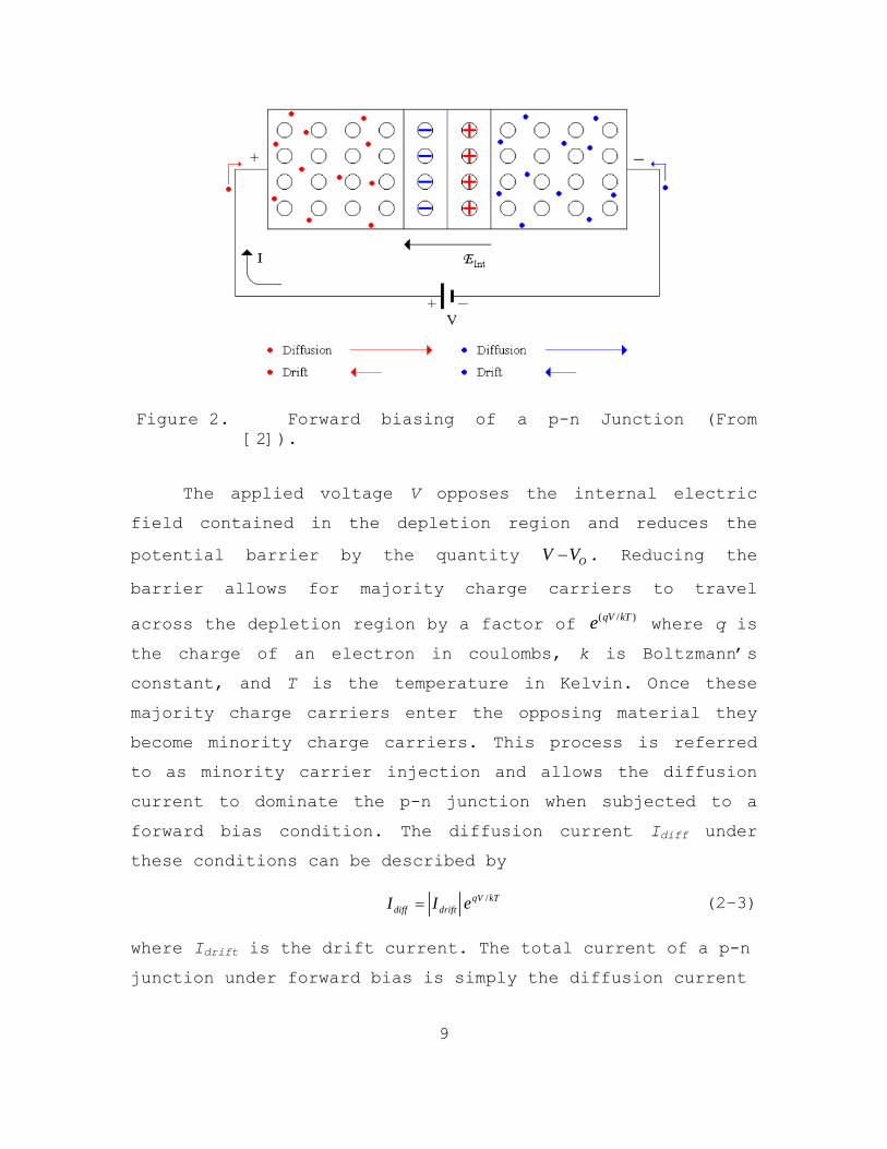
Figure 2. Forward biasing of a p-n Junction (From [2]).

The applied voltage V opposes the internal electric

field contained in the depletion region and reduces the

potential barrier by the quantity OV V . Reducing the

barrier allows for majority charge carriers to travel

across the depletion region by a factor of ( / )qV kTe where q is

the charge of an electron in coulombs, k is Boltzmann’s

constant, and T is the temperature in Kelvin. Once these

majority charge carriers enter the opposing material they

become minority charge carriers. This process is referred

to as minority carrier injection and allows the diffusion

current to dominate the p-n junction when subjected to a

forward bias condition. The diffusion current Idiff under

these conditions can be described by

/qV kTdiff driftI I e (2–3)

where Idrift is the drift current. The total current of a p-n

junction under forward bias is simply the diffusion current

10

minus the absolute value of the opposing drift current I0.

The total current I is given by

/0 1qV kTI I e (2–4)

which is also known as the ideal diode equation. Finally, a

more accurate diode equation can be found by substituting

the individual diffusion currents into Equation (2–4) and

solving for the minority injection currents to give

/ 1p qV kTnn p

p n

D DI qA p n e

L L

(2–5)

where Lp,n are the diffusion lengths of the holes and

electrons, pn and np are the minority charge concentrations,

and A is the area of the device.

3. Solar Radiation to Electric Energy

Each light photon that is absorbed by a semiconductor

that exceeds the material’s band gap has the potential to

generate an electron-hole pair (EHP). If the minority

carrier that results from an EHP diffuses towards the

depletion region, it will be swept to the opposite side by

the internal field. This will cause the drift current to

increase and a build-up of holes on the p-type

semiconductor and electrons on the n-type semiconductor.

This results in a forward bias condition for the p-n

junction, and the same diode current equations described in

Equations (2–4) and (2–5) can be used. The excess majority

charge carriers diffuse away from the depletion region and

oppose the diode current. The diffusion current is now

referred to as the photogeneration current IPh, and if an

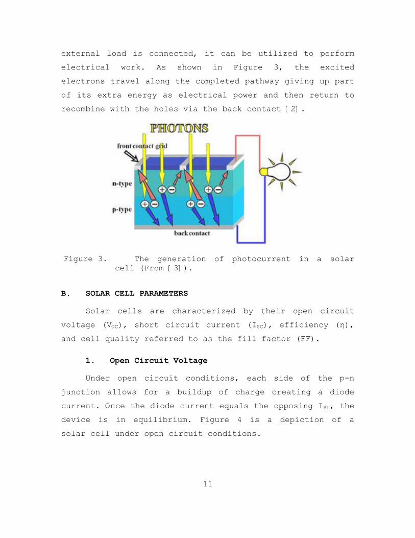
11

external load is connected, it can be utilized to perform

electrical work. As shown in Figure 3, the excited

electrons travel along the completed pathway giving up part

of its extra energy as electrical power and then return to

recombine with the holes via the back contact [2].

Figure 3. The generation of photocurrent in a solar cell (From [3]).

B. SOLAR CELL PARAMETERS

Solar cells are characterized by their open circuit

voltage (VOC), short circuit current (ISC), efficiency (η),

and cell quality referred to as the fill factor (FF).

1. Open Circuit Voltage

Under open circuit conditions, each side of the p-n

junction allows for a buildup of charge creating a diode

current. Once the diode current equals the opposing IPh, the

device is in equilibrium. Figure 4 is a depiction of a

solar cell under open circuit conditions.

12

Figure 4. The p-n junction under open circuit conditions VOC (From [2]).

2. Short Circuit Current

Under short circuit conditions, IPh is able to operate

at a maximum since there is no opposing diode current. The

IPh is proportional to the intensity of the sunlight that is

creating minority carriers from the EHPs. The ISC is at a

theoretical maximum when the cell is subjected to an ideal

solar intensity that only exists on the outside boundary of

the earth’s atmosphere. However, since solar cells are

predominantly used in less than ideal environments, a

practical ISC maximum is achieved during direct sunlight

conditions. Figure 5 is a depiction of a solar cell during

short circuit conditions.

13

Figure 5. The p-n junction under short circuit current conditions (From [2]).

The total current I of a solar cell is defined as the

diode current minus IPh and is described by

/0 ( )qv kT

PhI I e I . (2–6)

3. Efficiency and Fill Factor

The maximum output power Pout of a solar cell related

to the input power Pin that is generated by the photons

incident on a cell is a measure of its efficiency and is

described by

out

in

P

P . (2–7)

As described by

M M

SC OC

I VFF

I V , (2–8)

14

the FF is a measure of the quality of the solar cell and is

the ratio of the product of the maximum voltage VM and

current IM operating points that yield the maximum amount of

power to the product of VOC and ISC. Figure 6 is a depiction

of a current-voltage (I-V) curve for a solar cell. The

closer the I-V curve approaches the shape of a rectangle,

the higher the fill factor. Typical FFs for high quality

cells range from 0.75 to 0.85.

Figure 6. A typical I-V curve with MPP depicted (From [2]).

C. SOLAR CELL EFFICIENCY VARIABLES

A majority of the energy obtained from sunlight is

exhausted prior to ever reaching a PV cell by both internal

and external factors. These factors directly affect the

efficiency of the solar cell by governing how much solar

energy is actually converted into electrical energy.

15

1. Irradiance

Irradiance is defined as the amount of solar radiation

received per unit area on a particular surface [4].

Irradiance varies based the seasonal location of the earth

with respect to the sun, the position of sun in the sky

throughout a given day, and the weather [5]. The irradiance

of the sun at the boundary of our atmosphere is

approximately 1.360 kW/m2 and is referred to as the solar

constant, or air mass zero (AM0) [6]. The standard spectrum

of sunlight available at the earth’s surface in the

equatorial and tropical regions when the sun is directly

overhead is described as air mass one (AM1). Due to a

majority of the world’s population living at higher

latitudes than the equator and atmospheric attenuation

variables, the solar industry has agreed upon a standard

solar intensity of 1000 kW/m2, or AM1.5, to classify and

test solar panels [7].

2. Recombination

Direct and indirect internal recombination is the

elimination of charge carriers, both electrons and electron

holes, which occurs at the surface of the semiconductor, in

the bulk of the solar cell, and to a lesser extent, in the

depletion region. When recombination occurs at the surface

of the semiconductor, energy may be transferred into the

band gap causing electrons to fall back into the valence

band and recombine with holes. The effects of recombination

at the semiconductor surface can be mitigated by using

purer semiconductor materials. The other primary source of

electron-hole recombination occurs in the bulk of the

16

substrate and is caused by Auger recombination, Shockley-

Read-Hall recombination, and radiative recombination [7].

3. Temperature

Low energy photons (i.e., less than 1.1 electron volt

for silicon) will create heat that may lower cell

efficiency. Additionally, photons with too much energy will

create an EHP but will also increase cell temperature.

Lattice vibrations due to high or low temperatures

interfere with the flow of charges and results in non-

optimal operation. For silicon cells, there is an

approximate 2.3 mV per cell decrease in open-circuit

voltage when the temperature raises one Celsius [7]. In an

average solar cell, only 45% of incident photons are

converted to electrical energy. The remaining is dissipated

in the form of heat or pass through the material completely

[7].

4. Reflection

Reflection of light off the cell surface can be as

high as 36% for an untreated surface. The reflection

percentage can be reduced to around five percent through

the use of antireflection coatings (i.e., silicone oxide)

and surface texturing [7].

5. Electrical Resistance

There is resistance to charge and current flow in the

bulk of the case, in the surface, and at the contact

junction. Additionally, there is ohmic resistance in the

metal contacts that provide access to the p-n junction [7].

17

6. Material Defects and Self-shading

Dangling bonds from impurities and nonperfect crystal

structure causes recombination problems. Self-shading from

the top electric conductors causes photon reflection off

the top electrical grid and can result in losses up to

eight percent [7].

18


19

III. MAXIMUM POWER POINT TRAEQUATION CHAPTER (NEXT) SECTION 1CKERS

A. MPPT DESIGN PRINCIPLES

The wide-spread adoption of the utilization of solar

energy as a renewable resource is severely limited by the

relatively low conversion efficiency from solar to

electrical power. A general guideline for most PV systems

corresponds to an overall efficiency of less than 17% and

is significantly less under low irradiation conditions [8].

This low conversion attribute requires an almost

disproportionate quantity of solar cells to generate a

modest amount of useful electrical power. Therefore, any

device, technique, or advance in technology that increases

the energy conversion efficiency of a PV system by even a

small amount has a large impact in reducing the quantity of

cells and the physical size of the array. Other benefits of

optimizing the conversion efficiency include a significant

reduction in cost or a substantial increase in the power

available to the user.

A common method of maximizing the efficiency of a PV

system is the detection and tracking of an array’s MPP

under varying conditions. The MPP is not constant or easily

known; this is due to the nonlinear relationship between a

cell’s output and input variables (i.e., solar irradiation

and temperature) which results in a unique operating point

along the I-V curve where maximum power is delivered [9].

When a PV array is connected directly to the load, referred

to as a directly-coupled system, the overall operating

20

voltage of the system is determined by the intersection of

the load line and I-V curve as shown in Figure 7 [10].

Figure 7. The operating point of a directly-coupled PV

array and load (From [10]).

A fluctuating level of irradiance is one of the many

nonlinear variables that influence the I-V curve of a PV

array. As shown in Figure 8, the intersection of the load

line and varying I-V curves due to fluctuating irradiance

levels significantly impacts the operating voltage and

power output available to the load. The typical solution to

account for this nonlinear relationship is to oversize the

PV array to ensure the load’s power requirements are always

met.

21

Figure 8. A PV I-V curve at 40°C for different

irradiance levels (After [10]).

Although the cost per watt of solar energy has dropped

considerably, oversizing an array to account for the worst

case I-V curve is cost prohibitive for most applications.

An MPPT specifically addresses this scenario and provides a

cost effective solution. Simply put, an MPPT is a switch-

mode power converter that decouples the array from the load

to independently control the array’s voltage and current

[10]. A modern MPPT uses a micro-controller or analog

methods to locate the MPP by using calculation models or

more commonly, search algorithms. The proper names of these

methods include perturb and observe, incremental

conductance, fractional short circuit, fractional open

circuit voltage, fuzzy logic, neural networks, pilot cells,

and digital signal processor based implementations. Each of

these tracking algorithms has been written about

DC Load Line

22

extensively in the literature with varying levels of

effectiveness [8]. The more commonly used designs found in

commercial applications are summarized in this chapter.

B. ANALYSIS OF TRACKING ALGORITHMS

1. Perturb and Observe

The most common MPPT algorithm utilized is the perturb

and observe (P&O); this is due to its simplicity and ease

of implementation [10]. The basic premise behind P&O is the

algorithm’s constant comparison of the array’s output power

after a small, deliberate perturbation in the array’s

operating voltage is applied. If the output power is

increased after the perturbation, then the array’s

operating point is now closer to the MPP, and the algorithm

continues to “climb the hill” towards the MPP. If the power

is decreased, then the operating point is further from the

MPP, and the algorithm reverses the algebraic sign of the

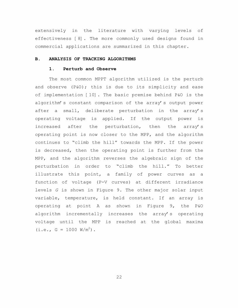
perturbation in order to “climb the hill.” To better

illustrate this point, a family of power curves as a

function of voltage (P-V curves) at different irradiance

levels G is shown in Figure 9. The other major solar input

variable, temperature, is held constant. If an array is

operating at point A as shown in Figure 9, the P&O

algorithm incrementally increases the array’s operating

voltage until the MPP is reached at the global maxima

(i.e., G = 1000 W/m2).

23

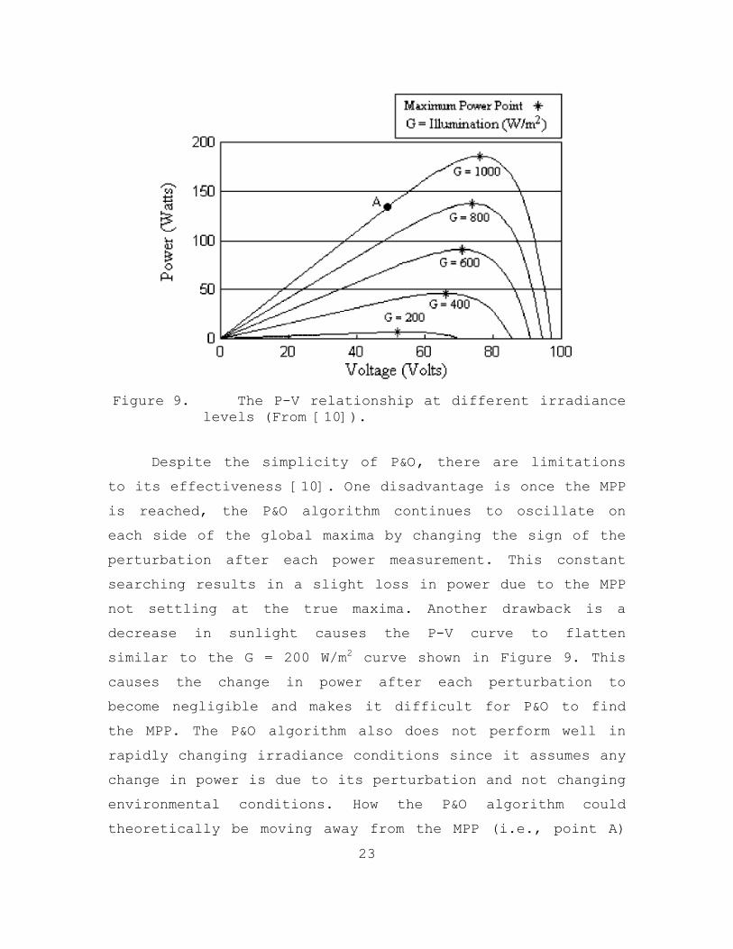
Figure 9. The P-V relationship at different irradiance

levels (From [10]).

Despite the simplicity of P&O, there are limitations

to its effectiveness [10]. One disadvantage is once the MPP

is reached, the P&O algorithm continues to oscillate on

each side of the global maxima by changing the sign of the

perturbation after each power measurement. This constant

searching results in a slight loss in power due to the MPP

not settling at the true maxima. Another drawback is a

decrease in sunlight causes the P-V curve to flatten

similar to the G = 200 W/m2 curve shown in Figure 9. This

causes the change in power after each perturbation to

become negligible and makes it difficult for P&O to find

the MPP. The P&O algorithm also does not perform well in

rapidly changing irradiance conditions since it assumes any

change in power is due to its perturbation and not changing

environmental conditions. How the P&O algorithm could

theoretically be moving away from the MPP (i.e., point A)

24

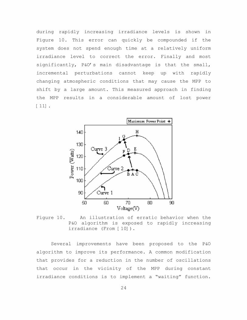
during rapidly increasing irradiance levels is shown in

Figure 10. This error can quickly be compounded if the

system does not spend enough time at a relatively uniform

irradiance level to correct the error. Finally and most

significantly, P&O’s main disadvantage is that the small,

incremental perturbations cannot keep up with rapidly

changing atmospheric conditions that may cause the MPP to

shift by a large amount. This measured approach in finding

the MPP results in a considerable amount of lost power

[11].

Figure 10. An illustration of erratic behavior when the

P&O algorithm is exposed to rapidly increasing irradiance (From [10]).

Several improvements have been proposed to the P&O

algorithm to improve its performance. A common modification

that provides for a reduction in the number of oscillations

that occur in the vicinity of the MPP during constant

irradiance conditions is to implement a “waiting” function.

25

A waiting function identifies when the algebraic sign of

the perturbation is reversed multiple times in a row. If

this condition is satisfied, the controller assumes it is

at the MPP and delays the perturbation process for a

defined period of time. This improves the efficiency of the

P&O controller during constant irradiance but also makes it

slow to respond when conditions do change [10]. Another

improvement takes two measurements that compare the array’s

power at a defined operating point separated by a time

interval; any change in the power indicates a fluctuating

level of irradiance and can be accounted for during the

perturbation process. However, these additional

measurements add complexity to the algorithm and make the

controller less responsive [10]. In summary, the operating

environment of the PV panel must be evaluated before any

modification to the original P&O algorithm is considered.

Each modification brings specific advantages that may or

may not offset any degradation to the overall system

efficiency.

2. Constant Voltage and Constant Current

The constant voltage (CV) algorithm is based on the

general observation that an array’s voltage at the maximum

power point VMPP compared to its open circuit voltage VOC can

be approximated based upon

1MPP

OC

VK

V (3–1)

where K is the predetermined value for the ratio [10]. The

flow chart in Figure 11 depicts the constant voltage

algorithm. In order to measure the open circuit voltage,

the solar array is temporarily isolated from the MPPT.

26

Given Equation (3–1) and the predetermined value K, the

MPPT adjusts the array’s voltage until VMPP is obtained.

This simple method is repeated periodically in order to

recalculate the VMPP and ensures the solar panel is

operating near its MPP.

Figure 11. A flowchart depicting the constant voltage

algorithm (From [10]).

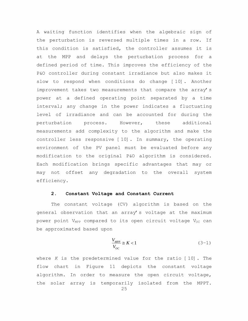
Literature recommends that the value for K should

range from 0.73 to 0.80. However, if the panel is exposed

to a range of temperatures (i.e., 0 to 60 C) and subjected

to varying irradiance levels (i.e., 200 to 1000 W/m2), it

becomes apparent that these variables affect the location

of the MPP, and the fixed ratio K is unable to adjust the

array’s VMPP. It can be seen in Figure 12 that K, depicted

on the y-axis, is dependent on environmental conditions.

Since K is a fixed, predetermined value, the error can

reach as high as eight percent in response to the

irradiance and temperature fluctuating [10].

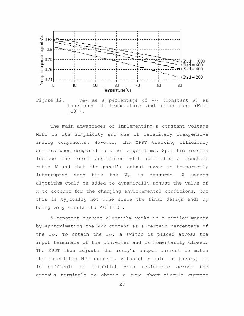
27

Figure 12. VMPP as a percentage of VOC (constant K) as

functions of temperature and irradiance (From [10]).

The main advantages of implementing a constant voltage

MPPT is its simplicity and use of relatively inexpensive

analog components. However, the MPPT tracking efficiency

suffers when compared to other algorithms. Specific reasons

include the error associated with selecting a constant

ratio K and that the panel’s output power is temporarily

interrupted each time the VOC is measured. A search

algorithm could be added to dynamically adjust the value of

K to account for the changing environmental conditions, but

this is typically not done since the final design ends up

being very similar to P&O [10].

A constant current algorithm works in a similar manner

by approximating the MPP current as a certain percentage of

the ISC. To obtain the ISC, a switch is placed across the

input terminals of the converter and is momentarily closed.

The MPPT then adjusts the array’s output current to match

the calculated MPP current. Although simple in theory, it

is difficult to establish zero resistance across the

array’s terminals to obtain a true short-circuit current

28

measurement. Thus, constant voltage MPPTs are preferred due

to the relative ease of measuring voltages vice short

circuit currents [10].

3. Pilot Cell

A pilot cell MPPT algorithm utilizes a small solar

cell called a pilot cell that has the same characteristics

as a larger PV array. The constant voltage or current

method is applied to the pilot cell in order to obtain the

VOC or ISC measurement. The calculated MPP can then be

applied to the larger array without the loss of power that

occurs during the VOC or ISC measurement. Disadvantages to

this method include utilizing a constant K that does not

adjust for temperature and irradiance fluctuations.

Additionally, the initial cost of the system is increased

due to the requirement that the characteristics of the

pilot cell must be calibrated to match the larger array

[10].

4. Incremental Conductance

The incremental conductance algorithm differentiates

the PV array power with respect to the voltage /dP dV and

then sets the result equal to zero [10]. If the PV array is

at the MPP, then the algorithm can be summarized by

( )

0dP d VI dI

I VdV dV dV

(3–2)

which can be rearranged to give

I dI

V dV (3–3)

29

where /dI dV is the current differentiated with respect to

the voltage. It is important to relate Equation (3–3) to

the incremental conductance algorithm. The left-hand side

of Equation (3–3) represents the array’s instantaneous

conductance, while the right-hand side represents the

incremental conductance [10]. At the MPP, these quantities

are equal to zero but contain the opposite sign. As the

array operating point moves away from the MPP, the set of

equalities given by

; 0dI I dP

dV V dV

(3–4)

; 0dI I dP

dV V dV

(3–5)

; 0dI I dP

dV V dV

(3–6)

can be used to define if the array is above or below the

operating point. Note that Equation (3–4) is the same as

Equation (3–3) but is repeated to signify the equilibrium

point of the algorithm (i.e., the MPP). Equations (3–5) and

(3–6) are used to determine the direction of the

perturbation to reach the equilibrium point. Once Equation

(3–4) is satisfied, the MPPT operates at this point until a

change of current is detected that is caused by a change in

the irradiance [10]. If 0dV and 0dI , then no

environmental changes have been detected and the MPPT is

operating at the MPP. If 0dV and the irradiance

increases, causing 0dI , then the MPP voltage also

increases. The MPPT will then increase the array’s

operating voltage to follow the rising MPP. If the

irradiance decreases, then 0dI , and the MPP voltage is

30

lowered causing the MPPT to decrease the array’s operating

point. Equations (3–5) and (3–6) are additionally used to

determine the direction of the voltage to reach the MPP if

the changes in the voltage and current are not zero. For

example, if / /dI dV I V , then / 0dP dV , and the operating

point is to the left of the MPP on the power versus voltage

curve. This will cause the MPPT to increase the array’s

operating voltage to reach the MPP. If / /dI dV I V , then

/ 0dP dV , and the operating point is now to the right of

the MPP on the power versus voltage curve. The MPPT will

reduce the array’s operating voltage to track the MPP. To

summarize, the incremental conductance algorithm can be

tedious due to its ability to adjust the array’s operating

point based on changes in the dV , /dI dV , or dI values.

This algorithm is depicted graphically using a flowchart as

shown in Figure 13.

The primary advantage of using incremental conductance

vice a P&O algorithm is its ability to calculate the

direction of the perturbation to reach the MPP and its

ability to determine when it actually reaches the MPP. This

characteristic is particularly useful during rapidly

changing irradiance conditions because incremental

conductance, unlike P&O, does not track in the wrong

direction and does not oscillate once it has arrived at the

MPP [10].

31

Figure 13. A flowchart of the incremental conductance

algorithm (From [10]).

5. Model-based Algorithm

A model-based algorithm can be utilized if the solar

cell parameters listed in the equation

exp 1L OSB

qI I I V IR

Ak T

(3–7)

are known. Equation (3–7) is referred to as the Shockley

equation for an illuminated p-n junction where A is the

diode ideality factor, q is the charge on an electron, and

R is the array’s series resistance. Additionally, IL is the

light-generated current as a function of G in W/m2, and IOS

is a function of the reference reverse saturation current.

If these values are known, then the solar cell’s current

and voltage can be calculated by measuring the value of

incident light and the temperature of the solar cell. Then

32

the VMPP can be calculated and set equal to the array’s

operating voltage. Although this algorithm is relatively

simple, its implementation is not realistic due to unknown

cell parameters that can change significantly with each

production run. Additionally, the light sensor (i.e.,

pyranometer) required to accurately measure the level of

irradiance causes model-based MPPT algorithms to be cost

prohibitive [10].

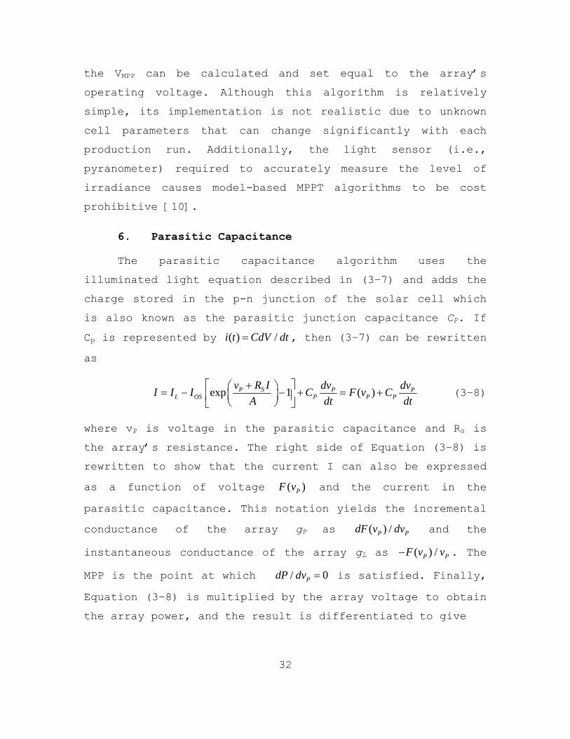
6. Parasitic Capacitance

The parasitic capacitance algorithm uses the

illuminated light equation described in (3–7) and adds the

charge stored in the p-n junction of the solar cell which

is also known as the parasitic junction capacitance CP. If

Cp is represented by ( ) /i t CdV dt , then (3–7) can be rewritten

as

exp 1 ( )P S P PL OS P P P

v R I dv dvI I I C F v C

A dt dt

(3–8)

where vP is voltage in the parasitic capacitance and Rs is

the array’s resistance. The right side of Equation (3–8) is

rewritten to show that the current I can also be expressed

as a function of voltage ( )PF v and the current in the

parasitic capacitance. This notation yields the incremental

conductance of the array gP as ( ) /P PdF v dv and the

instantaneous conductance of the array gL as ( ) /P PF v v . The

MPP is the point at which / 0PdP dv is satisfied. Finally,

Equation (3–8) is multiplied by the array voltage to obtain

the array power, and the result is differentiated to give

33

( ) ( )

0P PP

P P

dF V F VV VC

dV V V V

(3–9)

which represents the array’s power at the MPP. The

individual terms in Equation (3–9) represent the

instantaneous conductance, the incremental conductance, and

the ripple from the parasitic capacitance. Also note that

the first and second derivatives of the array voltage

encompass the AC ripple components generated by the

converter. It is important to note that if CP is equal to

zero, then the equation becomes synonymous with the

equation used for the incremental conductance algorithm.

Additionally, since Cp is modeled as a capacitor in parallel

with the individual cells, adding additional cells in

parallel will increase the capacitance as seen by the MPPT.

This translates to a significant difference in MPPT

efficiency between the parasitic capacitance and

incremental conductance algorithms when utilized in high-

power solar arrays with many modules [10].

In order to find the array’s conductance, a ratio is

established between instantaneous array current to the

instantaneous array voltage. Although more difficult, the

equation

1

2 2 2

1

12

12

i v i vn n n nn

GPP

v vOn nn

a a b bPg

V a b

(3–10)

can be used to obtain the array’s differential conductance

where GPP is the average ripple power, OV is the magnitude

of the voltage ripple, and , , , i v i vn n n na a b b are the coefficients

of the Fourier series of the PV array and current ripple

34

[10]. A circuit configuration as shown in Figure 14 can be

used to obtain the output values of GPP and 2OV , while the

inputs to the circuit are the array’s current and voltage.

The DC component of the array voltage is removed with the

high-pass filters, and the two multipliers create the AC

2OV ,or ( )ov t , and the AC GPP , or ( )GPp t , which are subsequently

filtered by the low pass filters to yield the DC components

of 2OV and GPP . From Equation (3–10), the ratio of these two

values is defined as the array’s conductance. The algorithm

then adjusts the array’s operating point until the array’s

conductance and differential conductance is equal.

Figure 14. The circuitry used when implementing the

parasitic capacitance algorithm (From [10]).

7. MPPT Algorithm Performance

Given the diversity of the various algorithms

described thus far, it is difficult to ascertain which

method is the best for maximizing an array’s output power.

Although a certain characteristic of one algorithm might

justify its exclusive use, most users of PV arrays are

concerned with the efficiency of the integrated system.

Therefore, a practical starting point would be to compare

35

the power output of an MPPT with the actual MPP of an array

that is being exposed to a constant temperature and level

of irradiance. A comparative study was conducted by [10] in

order to calculate the efficiency of a micro-controller

based MPPT using the following algorithms: P&O, incremental

conductance, and CV. The algorithms were loaded on

identical micro-controllers, optimized, and tested on

standardized hardware. It can be seen in Table 1 that the

efficiency of the P&O and incremental conductance Inc

algorithms are extremely high. As discussed previously, the

CV algorithm is the simplest to implement, but also results

in the lowest efficiency.

Table 1. Comparison of MPPT tracking efficiencies (ηMPPT) among selected algorithms (From [10]).

An updated and more in-depth study compared classical

P&O (P&Oa), modified P&O (P&Ob), three point weight

comparison P&O (P&Oc), CV, incremental conductance (IC),

open circuit voltage (OV), and short-current pulse (SC)

[8]. It is important to note that the different variations

of P&O all operate in a similar manner to the P&O algorithm

described in detail thus far. The minor modification among

them is in regards to their perturbation step-size. The

step-sizes are either constant (P&Oa), proportional to the

36

change in power (P&Ob), or averaged among three

perturbations (P&Oc). The experiment subjected the

different algorithms to changing irradiance levels of

either two levels (Case 1) or three levels (Case 2), and

the power output was captured once steady-state conditions

were reached. As shown in Table 2, the P&Ob algorithm

(i.e., a step-size proportional to the change in power)

provided the highest amount of energy output in Joules. It

is also important to note that classic P&O with a constant

step-size, defined as P&Oa, still produced acceptable

results [8].

Table 2. A comparative ranking of MPPT algorithms under varying irradiance inputs (From [8]).

C. ANALOG VERSUS DIGITAL MPPT DESIGN

1. Digital Design

Modern power management and renewable energy systems

are comprised of multiple subsystems that include power

sources, loads, power buses, and converter modules. The use

of MPPTs with digital algorithms offers many advantages

when interfacing with these subsystems. Digital methods

provide for data storage and transmission capabilities that

can help system maintenance and debugging. Additionally,

37

the degradation of components due to age or as a result

being exposed to harsh environments can lead to a loss of

accuracy for analog controllers [12]. On the complex end of

the digital design spectrum, implementing intelligent

algorithms such as fuzzy logic and neural networks allow

for adaptive control that provides for a responsive

controller but results in a cost-prohibitive commercial

application due to the additional hardware and computing

requirements. In order to realistically integrate digital

control into low-cost systems, most digital MPPT

controllers utilize a single, closed control loop that

manipulates the array input voltage in response to varying

environmental conditions. The P&O algorithm is by far the

most popular digital option due to its ease of

implementation and relatively good performance. Two

examples of digital P&O algorithms, classic and adaptive,

are compared in this section. However, classic P&O is not

explained in detail due to it being discussed at length

previously in this chapter. As a summary and a baseline for

the new method, classic P&O measures the change in power

via a closed control loop that uses a defined step-size to

perturb the duty cycle of the controller that results in a

small change in the operating point of the array. The

primary disadvantages to classic P&O are its slow and

possibly incorrect tracking direction when a rapid change

in the luminosity occurs [12]. To address the problem of

responsiveness, an adaptive P&O control strategy can be

implemented to speed up the tracking process. This ability

to easily modify microprocessor-based algorithms emphasizes

one of the strongest advantages of choosing digital control

over analog.

38

Adaptive P&O modifies the perturbation step-size so

that when the difference between the operating point and

the MPP is large, the step-size is also large. As the

algorithm starts to approach the MPP, it adjusts the step-

size to become very small [12]. While this method improves

upon the classic P&O approach, the adaptive P&O algorithm

can easily be modified to use two, independent control

loops to provide even more responsiveness to changing

environmental conditions. To better understand the

ingenuity of this approach, the concept of dual-control

loops will be explored and built upon.

The use of both a power control loop combined with a

voltage control loop keeps the adaptive P&O algorithm at a

fixed voltage during a rapid change in irradiance. This is

illustrated in Figure 15 by comparing the response of a

single, power control loop P&O algorithm (point A to B) to

the dual-control loop P&O approach (point A to C).

Figure 15. Change of current operating points when the

irradiance changes for different adaptive P&O algorithms (From [12]).

39

By preventing the MPPT from jumping to a greater

voltage and current (i.e., point B), the dual-control loop

algorithm holds the voltage constant and allows for a

change in the current in the same direction that the change

in irradiance occurred. The result is that point C is much

closer than point B, and the algorithm has less distance to

travel to reach the actual MPP (i.e., point D).

To address the problem of possibly tracking in the

wrong direction in response to a rapid luminosity change,

the dual-control loop P&O strategy can be slightly

modified. Instead of monitoring the voltage, the second

control loop now tracks the average solar panel input

current. In addition to increasing the tracking accuracy of

the MPPT, the average current control method produces three

other significant advantages:

The DC-DC converter acts as a current source, and the output is immune to voltage perturbations.

The current capability of the output can be increased by paralleling multiple converters.

Short-circuit protection is realized with the current loop [12].

Finally, a novel improvement to this approach combines

the average current control method with a variable step-

size algorithm that uses a hybrid of the fixed P&O and the

three-point P&O methods. As a side note, the three-point

method takes the average of three perturbations and adjusts

the step-size accordingly. The main advantage to using this

hybrid approach is that the complex calculation of

computing the slope of the P-V curve is not required in

order to determine the magnitude of the step-size. This

independence from the /dP dV calculation allows for this

40

scheme to be used with any solar panel without the

requirement to adjust the gain of the current and voltage

sensors [12]. Experiments for this novel adaptive P&O

algorithm show changes in irradiance resulted in the new

MPP being reached in 1.2 seconds [12]. Compared to classic

P&O, this adaptive approach provides for a faster transient

response time, and the overall time to converge at the MPP

is reduced by a factor of two.

The primary conclusion from this section is the

performance characteristics of a modern, digital P&O

controller that significantly improved upon most of the

disadvantages of classic P&O (i.e., response time and

tracking error). The 1.2 seconds it takes to reach the MPP

represents the best response time of current P&O algorithms

and should be used as a general reference during system

design.

2. Analog Design

Analog MPPT control strategies are enjoying a

reemergence in popularity due to their simplicity, cost

effectiveness, and low power requirements. A common

strategy when designing an analog MPPT is to utilize a

comparator to detect changes in the load current. An analog

controller utilizing a load current-based control strategy

can be easily integrated into the power converter circuitry

as shown in the block diagram of Figure 16. The DC-DC

converter regulates the voltage and current of the PV panel

and, therefore, controls the output power. The analog MPPT

controller continuously adjusts the duty cycle of the power

converter to ensure the MPP of each panel/cell is achieved

[13]. Although the analog algorithms described in this

41

section each track the MPP in a different manner, they are

all comprised entirely of analog components and are

dependent on comparing changes in the load current after an

input variable is modified. Two examples of analog control

are explained in further detail below and were chosen due

to their popularity and ingenuity, respectively.

Figure 16. A PV System with a load current-based analog

MPPT controller (From [13]).

a. Analog Perturb and Observe of the Load Current

Forced changes in the load current are caused by

a P&O control strategy that continuously adjusts the duty

cycle of the controller while observing the output current.

As long as the output current increases due to the

disturbance, the next disturbance should be in the same

direction. A simulation of a simple P&O analog controller

has successfully demonstrated load current comparison by

increasing the load current (i.e., delivering more power to

the load) as the PV panel generates more power due to

increasing irradiance levels [13]. The simplicity and the

relatively few components required to implement a load

current based control strategy for an analog MPPT is shown

in Figure 17.

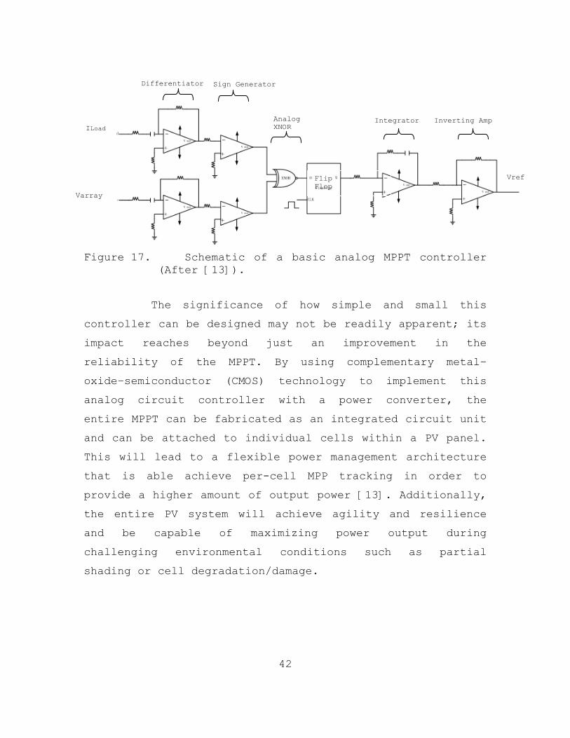
42

Figure 17. Schematic of a basic analog MPPT controller

(After [13]).

The significance of how simple and small this

controller can be designed may not be readily apparent; its

impact reaches beyond just an improvement in the

reliability of the MPPT. By using complementary metal–

oxide–semiconductor (CMOS) technology to implement this

analog circuit controller with a power converter, the

entire MPPT can be fabricated as an integrated circuit unit

and can be attached to individual cells within a PV panel.

This will lead to a flexible power management architecture

that is able achieve per-cell MPP tracking in order to

provide a higher amount of output power [13]. Additionally,

the entire PV system will achieve agility and resilience

and be capable of maximizing power output during

challenging environmental conditions such as partial

shading or cell degradation/damage.

Differentiator

Analog XNOR

Sign Generator

Integrator Inverting Amp

Flip Flop

Vref

ILoad

Varray

43

b. TEODI

Technique based on Equalization of the Output

operating points in correspondence of the forced

Displacement of the Input operating points of two identical

systems (TEODI) is a newer analog MPPT technique that is

simpler than digital methods, requires no memory and

multiplication operations, and still provides a high level

of efficiency when compared to P&O methods. The main

advantages of utilizing TEODI to detect the MPP are the

following [14]:

Implementation is simple and there is no need for a digital microprocessor.

It does not require a measurement of the PV panel’s current and voltage.

Since the PV panel’s power output is not tracked, this leads to a simpler controller design with fewer components. Less components increase reliability.

It can be used with any type of power converter technology.

A very high efficiency can be achieved since there are no fluctuations at the PV operating point.

When connecting to the power grid, the 60 Hz disturbances that may cause a failure in the P&O algorithm are avoided when using TEODI.

TEODI is applicable to distributed MPPT operations.

TEODI was originally designed for applications

that utilize two identical PV modules operating under the

same levels of irradiance and temperature [14]. The optimal

application of TEODI is when a PV module is divided into

identical submodules that share a single integrated MPPT

44

controller. However, although an integrated MPPT controller

is used, each submodule has its own DC-DC converter. The

TEODI approach forces the submodules to operate at the same

output voltage since they are operating in parallel with

respect to the load. The basic principle behind TEODI is

that since the output voltages are the same and the

currents produced by the submodules are also identical due

to the irradiance and temperature being uniform for both

sub modules, the input power of the two DC-DC converters

must also be the same value. This can only occur in two

cases:

Case 1) if the input operating voltages of the

two submodules are the same value

or

Case 2) if the two sub modules are producing the

same power, but the input operating voltages vA1 and vB1

are located at opposite sides of the MPP as shown in Figure

18 [14].

Figure 18. Location of TEODI case 2 operating points on

a notional P-V curve (From [13]).

45

TEODI is able to track and operate at the MPP by

ensuring the PV system always operates in the second

condition stated above. The TEODI tracking algorithm

constantly samples the power output of the submodules and

makes adjustments to the input voltage operating points

until equalization of the output power is achieved.

Although the voltage operating points of the submodules are

exaggerated in Figure 18 to illustrate a point, they are in

actuality very close to the MPP which results in a high

overall system efficiency. Comparing TEODI to an optimized

P&O algorithm results in a nearly identical power output at

steady state, but it can be shown that a higher tracking

speed is achieved using TEODI [14].

In order to achieve the highest efficiency, TEODI

requires the differences between the power and voltage

characteristics of the submodules to be negligible [14].

The obvious problem with this requirement is that

manufacturing identical sub modules that are simultaneously

exposed to the same irradiance and temperature is nearly

impossible to achieve in practical applications. However, a

small modification to the original TEODI design will allow

for the algorithm to account for mismatched operating

conditions. This is accomplished by the addition of a peak

detector that compares the magnitude of the individual

output currents and forces the system to operate at the MPP

regardless of fluctuating input variables. The addition of

a peak detector is inexpensive and requires few analog

components; thus, the simplicity and reliability of TEODI

is maintained [14].

46

D. MPPT CONVERTER TECHNOLOGY

The theory behind power conversion is quite varied and

can be extremely complex depending on the requirements of

the application. The approach required to boost AC voltage

in preparation for its journey across hundreds of miles of

transmission lines is quite different than the switch-mode

inductor converters found in modern, battery-operated

electronics. This section purposely avoids a lengthy review

of the numerous types of power conversion techniques and

the theory behind them. Additionally, although the use of

inverters are an important component of large-scale PV

systems that directly feed the commercial grid, most users

rely on a DC storage element to provide flexibility and

control when the PV power is utilized. Therefore, the goal

of this section is to focus primarily on inductively fed,

switch-mode converters in order to familiarize the reader

with the principal DC-DC converter technology used in

modern PV system design.

1. Inductively Fed, Switch-mode DC-DC Converters

Inductively fed, switch-mode DC-DC converters are used

almost exclusively in portable devices where system size

and efficiency are the primary design factors. Size and

efficiency also govern the use of multiple MPPTs at the

sub-panel level and is instrumental in the ultimate

realization of assigning an MPPT to each individual solar

cell within a PV system. Although numerous DC-DC converter

methods are available, switch-mode converters are primarily

discussed due to their almost exclusive use in commercially

available MPPTs.

47

Regardless of whether the input DC voltage is being

increased (i.e., boost converter) or decreased (i.e., buck

converter), the mechanisms responsible for the energy

losses in a switch-mode converter are the same. They

include the components responsible for conduction,

capacitor-drive, and quiescent power [15]. The primary

problem with reducing the physical size of a CMOS based

switch-mode converter is the resulting decrease in

efficiency. However, advances in finer CMOS technologies

that capitalize on shorter minimum channel lengths, higher

oxide capacitance, and lower breakdown voltages have

resulted in a promising potential for reducing the size of

switch-mode converters. For example, a study of CMOS buck

converters demonstrated that when varying channel lengths

of 0.18 µm, 0.35 µm, and 0.50 µm were optimized, they

yielded efficiencies of 93%, 89%, and 79%, respectively.

Additionally, this was independent of the converter’s

operation whether in a continuous conduction mode CCM or a

discontinuous conduction mode DCM. This study concluded

that finer pitched technologies yielded higher efficiency

as long as leakage current, which often increases with

reductions in pitch, does not become a significant portion

of the load [15].

This study allows us to assume that improved

manufacturing processes will provide a path forward for

switch-mode converters to maintain high efficiencies (i.e.,

greater than 90%) as they shrink. Compared to linear

converters, switch-mode converters also maintain a

relatively high efficiency when a large voltage

differential exists between the input and output. However,

as shown by the efficiency curve in Figure 19, this

48

characteristic does not apply to operating the converter at

low or high loads [16]. While industry has created a “soft

switching” technique to improve the performance at low

loads (i.e., a standby or sleep state), the PV system

designer is mostly concerned with maximizing the power from

a solar array. Therefore, MPPT applications require a

switch-mode converter that is rated at a higher current

capacity than necessary to avoid the decrease in efficiency

when the converter is heavily loaded. Due to the inductor

being the most expensive, largest, and heaviest component

of an inductively fed, switch-mode converter, this creates

a design tradeoff of gaining improvements in efficiency at

the expense of cost, weight, and size.

Figure 19. A typical efficiency curve of an inductively

fed, switch-mode DC/DC converter (From [16]).

As a possible solution to problem, recent research

indicates that integrated, capacitively fed switch-mode

converter can achieve respectable performance compared to

an inductively fed switch-mode converter of similar

capability. This capacitive switch-mode converter operates

very similarly and is able to offer both high efficiency

and high power density while avoiding the use of thick

49

metals and magnetic materials that an inductively fed

converter must rely on. Due to the savings in weight and

size, these advances in capacitor-based converters are of

particular interest to integrating MPPTs at the individual

solar cell level. The study concluded that capacitor

converters had a “bright future” for high power density

integrated DC-DC converters [17].

2. MPPT Converter Design

For purposes of PV system design, it is important to

gain a perspective on the size of current converter

technology. A 300 watt digital P&O MPPT with an inductively

fed, switch-mode boost converter is shown in Figure 20. The

reader should note that:

This is a demonstration board provided by the manufacturer and could be shrunk considerably if produced commercially.

It is capable of 300 watts where per cell applications of MPPTs would only require a few watts.

As discussed previously, overall MPPT size is primarily determined by the switch-mode converter. This is validated by finding the inductors labeled L1-L4, which also happen to be the largest components on the board.

Using the size of this MPPT and its intended use for

larger-scale PV system applications as a reference, we see

that it is well within reason to assume that foreseeable

advances in DC-DC converter technology will allow for the

assignment of an MPPT to each individual cell without

significantly impeding the surface area of the array. An

ideal example of this per cell application would be if a

simple analog MPPT controller and converter was placed

directly the beneath solar cell and the electrical

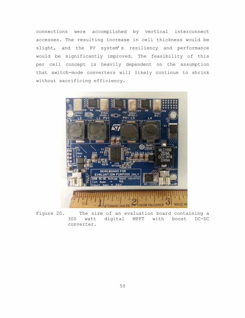
50

connections were accomplished by vertical interconnect

accesses. The resulting increase in cell thickness would be

slight, and the PV system’s resiliency and performance

would be significantly improved. The feasibility of this

per cell concept is heavily dependent on the assumption

that switch-mode converters will likely continue to shrink

without sacrificing efficiency.

Figure 20. The size of an evaluation board containing a

300 watt digital MPPT with boost DC-DC converter.

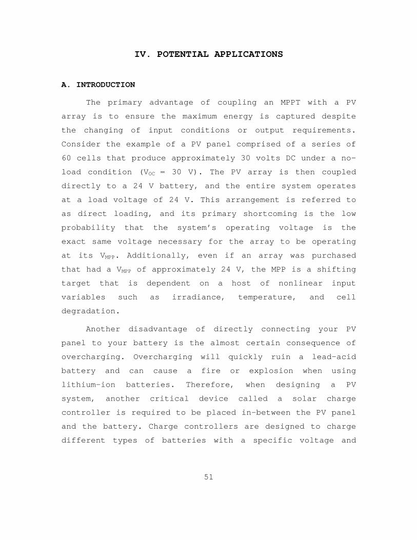
51

IV. POTENTIAL APPLICATIONS

A. INTRODUCTION

The primary advantage of coupling an MPPT with a PV

array is to ensure the maximum energy is captured despite

the changing of input conditions or output requirements.

Consider the example of a PV panel comprised of a series of

60 cells that produce approximately 30 volts DC under a no-

load condition (VOC = 30 V). The PV array is then coupled

directly to a 24 V battery, and the entire system operates

at a load voltage of 24 V. This arrangement is referred to

as direct loading, and its primary shortcoming is the low

probability that the system’s operating voltage is the

exact same voltage necessary for the array to be operating

at its VMPP. Additionally, even if an array was purchased

that had a VMPP of approximately 24 V, the MPP is a shifting

target that is dependent on a host of nonlinear input

variables such as irradiance, temperature, and cell

degradation.

Another disadvantage of directly connecting your PV

panel to your battery is the almost certain consequence of

overcharging. Overcharging will quickly ruin a lead-acid

battery and can cause a fire or explosion when using

lithium-ion batteries. Therefore, when designing a PV

system, another critical device called a solar charge

controller is required to be placed in-between the PV panel

and the battery. Charge controllers are designed to charge

different types of batteries with a specific voltage and

52

current profile that prevents damage and improves the

performance of the energy storage system.

The three components described thus far are simple,

relatively inexpensive, and reliable. It is no surprise

that they comprise a majority of the PV systems in use

today. Unfortunately, these same PV arrays either fail to

operate at their maximum potential or as a deliberate work-

around, the arrays are oversized in order to guarantee a

certain amount of power is delivered to the load. However,

oversizing an array is an expensive solution when using

high quality solar cells or may be impossible with respect

to applications that have limited surface area (i.e.,

satellites). Thus, when designing a more sophisticated PV

system, the motivation for using an MPPT reaches beyond

just the extra power that is gained when the array is

forced to operate at its true potential. A relatively

inexpensive MPPT can save thousands of dollars when large

arrays are built or can make the difference between a

sensor being included on a satellite or not. Modern MPPTs

are small, efficient, and are becoming so inexpensive the

PV industry is not just using one MPPT per array but

assigning an MPPT to each sub-panel within an array.

B. A CASE FOR MULTIPLE MPPTS

Consider the 30 V DC panel mentioned previously is now

connected in series to other panels to effectively create a

single array capable of producing an output rating of 300 V

DC. This array is connected to an MPPT, and its output is

run through an inverter which converts it to standard AC

voltage for household use. Arranging the PV system in this

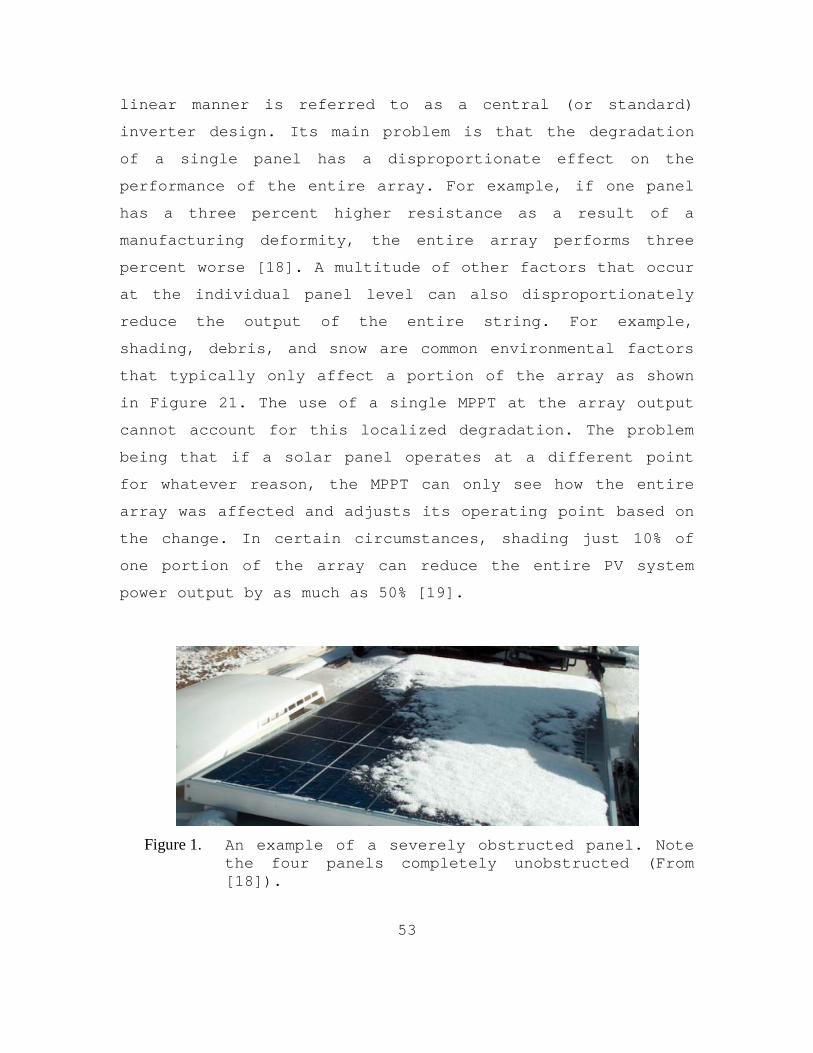
53

linear manner is referred to as a central (or standard)

inverter design. Its main problem is that the degradation

of a single panel has a disproportionate effect on the

performance of the entire array. For example, if one panel

has a three percent higher resistance as a result of a

manufacturing deformity, the entire array performs three

percent worse [18]. A multitude of other factors that occur

at the individual panel level can also disproportionately

reduce the output of the entire string. For example,

shading, debris, and snow are common environmental factors

that typically only affect a portion of the array as shown

in Figure 21. The use of a single MPPT at the array output

cannot account for this localized degradation. The problem

being that if a solar panel operates at a different point

for whatever reason, the MPPT can only see how the entire

array was affected and adjusts its operating point based on

the change. In certain circumstances, shading just 10% of

one portion of the array can reduce the entire PV system

power output by as much as 50% [19].

Figure 1. An example of a severely obstructed panel. Note the four panels completely unobstructed (From [18]).

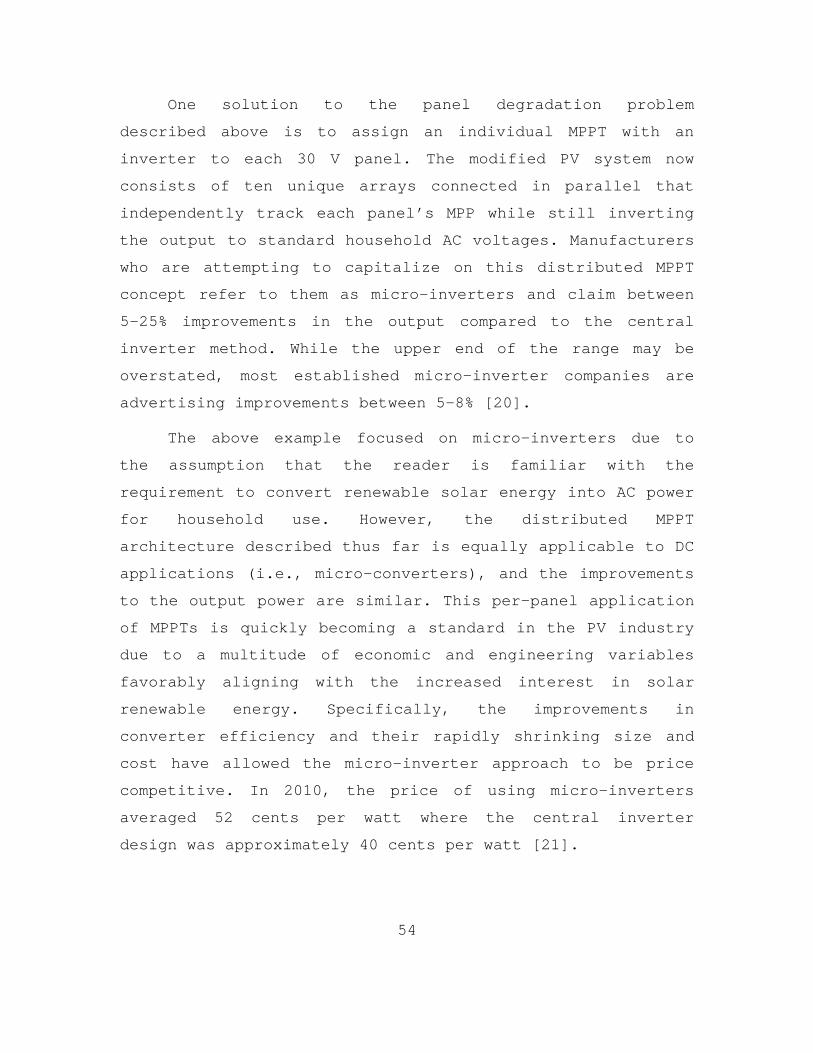
54

One solution to the panel degradation problem

described above is to assign an individual MPPT with an

inverter to each 30 V panel. The modified PV system now

consists of ten unique arrays connected in parallel that

independently track each panel’s MPP while still inverting

the output to standard household AC voltages. Manufacturers

who are attempting to capitalize on this distributed MPPT

concept refer to them as micro-inverters and claim between

5–25% improvements in the output compared to the central

inverter method. While the upper end of the range may be

overstated, most established micro-inverter companies are

advertising improvements between 5–8% [20].

The above example focused on micro-inverters due to

the assumption that the reader is familiar with the

requirement to convert renewable solar energy into AC power

for household use. However, the distributed MPPT

architecture described thus far is equally applicable to DC

applications (i.e., micro-converters), and the improvements

to the output power are similar. This per-panel application

of MPPTs is quickly becoming a standard in the PV industry

due to a multitude of economic and engineering variables

favorably aligning with the increased interest in solar

renewable energy. Specifically, the improvements in

converter efficiency and their rapidly shrinking size and

cost have allowed the micro-inverter approach to be price

competitive. In 2010, the price of using micro-inverters

averaged 52 cents per watt where the central inverter

design was approximately 40 cents per watt [21].

55

Although a higher price per watt is a significant

disadvantage to the micro-inverter approach, additional

benefits may make up the difference. They include:

• Higher reliability–Since micro-inverters are not subjected to as high power and heat loads, they last longer. Manufacturers typically offer warranties of 20–25 years for micro inverters and 10–15 years for central inverters.

• Flexibility in future requirements–Expansion of the micro-inverter system is cost effective since each panel operates independently. Central inverters would require a second large inverter to be installed and possibly the rewiring of the existing panels.

• Distributed approach–Micro-inverters prevent localized disruptions from affecting the entire system. If something is wrong with a solar panel or the corresponding micro-inverter, the rest of the system is unaffected.

• Safety–Central inverters typically require higher voltage wiring to handle the 300–600 V DC voltage potential that results from connecting panels in series. Micro-inverters improve safety by eliminating the need for high voltage wiring since each panel is inverted and directly tied to the AC grid.

• Noise–Central inverters may require active cooling (i.e., fans) to dissipate large amounts of heat. Micro-inverters utilize passive-cooling.

Despite these numerous benefits, some applications

still do not justify the added expense. For example,

consider the case of a homogeneous PV system (i.e., similar

panels) that is equally subjected to the same input

conditions as shown in Figure 22. Although minor

degradations would still be present between each panel,

most of the system would operate at a similar MPP. While

some advantages of the micro-inverter method are still

56

relevant, the resulting power output between the two

approaches would be very similar, making the decision to

use a central or micro-inverter approach much less

straightforward.

Figure 2. An example of a homogeneous array exposed to similar environmental conditions.

Keeping this example in mind, generalized

recommendations about the use of micro-inverters can be

made to the PV system designer. First, micro-inverters

excel when portions of the array are being subjected to a

dynamic range of input conditions. Second, micro-inverters

should be used when a degree of resiliency is desired in

the system. In other words, by operating independently,

degradation or failure of one panel does not

disproportionately affect the performance of the entire

array. Finally, micro-inverters should be used when system

longevity is a primary concern or when access to the array

is difficult. Micro-inverters typically outlast large

central inverters and can extend the service life of

specialized applications such as satellite systems. The

57

examples outlined in the remaining sections of this chapter

are hypothetical scenarios that the author suggests could

benefit from the use of multiple MPPTs.

C. SPACE APPLICATIONS

The Petite Amateur Navy Satellite PANSAT was a

“tumbler” satellite designed and built at the Navy

Postgraduate School with the aim of providing a small, low-

cost, spread spectrum communication satellite for message

relay. The satellite was launched by the space shuttle in

1988, and an image of the satellite is shown in Figure 23.

Its power system specifications include:

• 17 panels available (total area of 1209 cm2).

• Each panel has 32 silicon cells connected in series for primary power. A minimum efficiency of 14.5% at AM0 and 28C is required.

• Nickel-cadmium batteries for eclipse power.

• 12 V DC bus voltage.

• 10 W end-of-life power requirement.

Figure 3. An image of PANSAT (From [22]).

58

Although this satellite is in constant rotation once

deployed, this example focuses on the power available at a

specific moment in time. For the following calculations,

the top of the satellite is normal to the sun as depicted

in Figure 24. In this orientation, the center panel

receives the full irradiance available from the sun, while

the four surrounding panels are situated at a 45⁰ angle. As

a general rule, if a surface is not normal to the sun, the

solar irradiance falling on it will be reduced by the

cosine of the angle between the surface normal and the

incident ray.

Figure 4. Top view of the PANSAT satellite (From [22]).

1. Direct Loading Versus Central Converter Approach

The performance of the five panels wired together in

parallel (i.e., a single array) can be represented by the

hypothetical I-V curve shown in Figure 25.

59

Figure 25. Hypothetical I-V response curve of a PANSAT

satellite wired as a single array.

When the single array configuration is subjected to

direct loading, the power delivered is approximated by

outP ( )( ) (12 )(0.86 ) 10.32Load LoadV I V A W (4–1)

where the operating voltage VLoad and current ILoad are

obtained by identifying where the 12 V load line intersects

the I-V curve as seen in Figure 25. When the system is

configured for use with a single MPPT that has an

efficiency of approximately 94%, the power delivered is

approximated by

out .P ( )( ) 0.94 (13.2 )(0.80 ) 9.93conv MPP MPPV I V A W (4–2)

where the values are obtained by multiplying the efficiency

of the MPPT by the MPP of the array.

60

Clearly, the use of a single MPPT, or central

converter, is not feasible since the minimum end-of-life

power requirement of 10 W is not met. While this example is

extremely limited in its scope, the designers of PANSAT

purposely designed their array to deliver a MPP around the

expected 12 V load requirement. When using a single MPPT,

the approximate six percent loss that results from the

algorithm tracking error and DC-DC conversion process is

greater than the minor loss of power that results from

operating the array near, but not at, the VMPP under the

direct loading method. However, recall that a single MPPT

cannot identify localized problems within the array. In

most instances, it only takes one moderately degraded panel

to disproportionately affect the entire system. In an

attempt to lessen the effects of dissimilar irradiance

levels, in the next section the use of micro-converters to

treat each panel separately in order to outperform the

direct loading method is considered.

2. Micro-converter Approach

The effects of treating each panel separately can be

represented by the hypothetical I-V curves shown in Figure

26. Note that the solid curved line represents the top

panel that is normal to the source, while the dotted curve

line represents the four offset panels being exposed to

uniformly smaller irradiance levels (i.e., the dotted line

is actually four overlapping lines). It can be seen that

the MPP of the top panel is 12.7 V which is relatively

close to the load voltage of 12 V. However, the four offset

panels have a MPP of 14.1 V and are operating 2.1 V below

their true potential under the direct loading method.

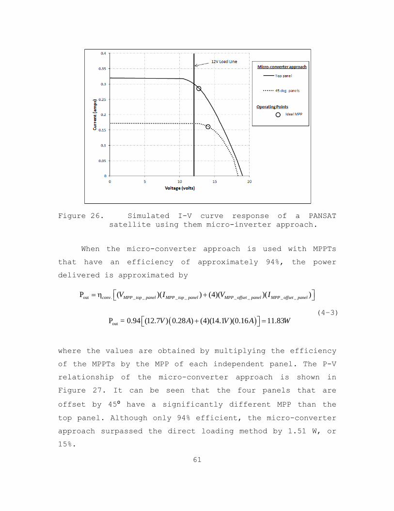
61

Figure 26. Simulated I-V curve response of a PANSAT

satellite using them micro-inverter approach.

When the micro-converter approach is used with MPPTs

that have an efficiency of approximately 94%, the power

delivered is approximated by

out . _ _ _ _ _ _ _ _

out

P ( )( ) (4)( )( )

P = 0.94 (12.7 ) 0.28 ) (4)(14.1 )(0.16 11.83

conv MPP top panel MPP top panel MPP offset panel MPP offset panelV I V I

V A V A W

(4–3)

where the values are obtained by multiplying the efficiency

of the MPPTs by the MPP of each independent panel. The P-V

relationship of the micro-converter approach is shown in

Figure 27. It can be seen that the four panels that are

offset by 45⁰ have a significantly different MPP than the

top panel. Although only 94% efficient, the micro-converter

approach surpassed the direct loading method by 1.51 W, or

15%.

62

Figure 27. Simulated P-V curve response of a PANSAT

satellite using the micro-converter approach.

The purpose of this example was to provide a practical

demonstration of using the multiple MPPT approach. The

PANSAT satellite is an ideal illustration of individual

panels being exposed to drastically different input

conditions. However, for simplicity’s sake, this example

infers the use of certain ideal characteristics of MPPTs

and ignores the rotating aspect of PANSAT. When designing

with MPPTs, each tracking algorithm and conversion method

has its disadvantages that may render the use of MPPTs

impractical. Applying this logic to PANSAT, we see that

using a P&O MPPT that has a relatively slow tracking

algorithm may not be beneficial if the rotating “tumbler”

satellite exceeds the MPPT’s tracking capabilities.

However, innovations and decreasing prices in the solar

63

industry is enabling a revolution in the type of

applications suitable for solar cells. No longer is the use

of solar cells reserved for highly specialized applications

where solar power is the only practical long-term energy

solution. As outlined in the next section, solar cells are

currently being used in applications that just a few years

ago would have been impossible due to the cost and weight

of traditional silicone cells. Thus, it is expected that

the traditional use of MPPTs will also evolve and their

strengths and weaknesses must be considered to ensure

desired performance is met.

D. MILITARY APPLICATIONS

Two current examples of military applications where

using multiple MPPTs may be beneficial are presented in

this section. Recall, the multiple MPPT design principles

suggested in Chapter III are still applicable.

Specifically, the micro-converter approach excels when

portions of the array are subjected to significantly

different input conditions and/or when a high degree of

system resiliency is desired.

1. Tactical Solar Tents and Shelters

Until recently, traditional solar panels were

comprised of crystalline silicone cells that are housed in

a metal frame and protected with a glass cover. These

traditional solar panels were rigid, expensive, and heavy.

However, recent advances in amorphous silicon cells,

otherwise known as thin film technology, has increased the

efficiency of flexible cells from approximately six percent

to 14% [23]. This large increase in efficiency has provided

64

for the development of numerous thin-cell applications that

meet the military’s requirements for ruggedness and power

output. For example, the Tactical Solar Tent from Energy

Technologies, Incorporated, shown in Figure 28, can provide

up to 190 watts of solar power for each 8’ x 9’ shelter

section. However, similar to the 45° offset panels on

PANSAT, the solar panels on the tent that are not normal to

the sun disproportionately reduce the performance of the

entire PV system. It is safe to assume that real-world

applications of tactical solar blankets and tents will

result in non-ideal PV array configurations such as

depicted in Figure 28. Additionally, tactical applications

are especially vulnerable to localized disruptions such as

shading or cell damage due to the dynamic environment they

will be operating in. The micro-converter approach would be

beneficial by allowing each panel to operate at its MPP

while providing a greater degree of reliability and

durability.

Figure 28. The Energy Technologies, Inc. Tactical Solar

Tent (From [23]).

65

2. Unmanned Aerial Vehicles

The same advances in thin film solar cells that have

made tactical solar blankets and tents practical can also

be used in other military applications. For example, the

military and other government agencies have bought tens of

thousands of unmanned aerial vehicles UAVs of varying sizes

in the past ten years. A significant disadvantage to UAVs,

particularly smaller platforms, is their short flight time

due to a lack of a lightweight, high-capacity energy

source. The AeroVironment Raven RQ-11 platform shown in

Figure 29 is an example of a smaller UAV that has

approximately 60–90 minutes of flight endurance before its

batteries are exhausted.

Figure 29. The AeroVironment Raven RQ-11 UAV

(manufacturer’s image).

Experiments have shown that the flight endurance of

the Raven RQ-11 can be dramatically increased with the

addition of copper indium gallium selenide (CIGS) solar

cells [24]. However, these experiments placed CIGS cells

only on the top surface of the main wing assembly. This was

primarily due to the fact that the top of the main wing

assembly presents the only large surface area that is

66

exposed to relatively uniform irradiance conditions. Thus,

placing CIGS cells on smaller, shaded areas of the UAV

(i.e., the vertical stabilizer) could significantly

decrease the performance of the main wing array. Similar to

previous examples, the micro-converter approach would be

particularly useful due to the different surfaces of the

UAV being exposed to a dynamic range of irradiance levels.

This is further complicated by the constant banking and

turning that occurs in flight. The use of micro-converters

would allow for almost every square inch of the Raven to be

covered in thin film cells resulting in multiple panels. In

addition to each panel tracking its MPP independently, each

DC converter could be customized to allow for greater

flexibility in meeting the Raven’s charging requirement of

approximately 25 V. This is especially applicable to

smaller areas of the Raven where arranging 48 cells in

series (VOC > 25 V) is not practical.

67

V. TEST AND DATA ANALYSIS

A. INTRODUCTION

This primary goal of testing is to evaluate the

multiple MPPT approach and to validate an increase in the

efficiency compared to direct loading or a central

converter. The individual MPPT and solar panel selection

process that was conducted prior to integrating the final

PV system for testing is discussed in this chapter. Once

the system was integrated, tests were carried out to

evaluate the performance of the system during varying

levels of irradiance under direct loading, central-

converter, and micro-converter arrangements. Finally, the

data was analyzed and general observations were made about

the use of multiple MPPTs.

General equipment utilized throughout testing are

discussed in the following subsections.

1. Amprobe Solar 600 Analyzer

The I-V and P-V characteristics of the solar panels

are obtained with the Amprobe Solar-600 analyzer. This

analyzer, shown in Figure 30, is a high-quality diagnostic

device capable of testing and determining the operating

characteristics of solar panels [24]. The solar panel being

analyzed is subjected to VOC, ISC, and numerous operating

points in between to create an exportable spread sheet of

data that can be used to plot the I-V and P-V

relationships. Additionally, the VMPP of the panel is

identified which can be used to determine if the MPPT is

68

properly tracking the MPP. An example of the data exported

from the Solar-600 is shown in Appendix B.

Figure 30. The Amprobe Solar-600 Analyzer (From [24]).

2. Radiant Source Technology (RST) Solar Simulator

The RST Solar Simulator is a light source for use in

the testing of solar cells, sun sensors, and other small

devices. The simulator, shown in Figure 31, has the

following output capabilities [25]:

Output Beam: 12” x 12”

Lamp Power: 3000 W

Air Mass Capability: AM0

Cooling: Forced air

Classification: ABA ASTM E927

Spectral match, class A, 0.75–1.25

Non-uniformity of irradiance, class B, ≤5%

Temporal instability, class A, ≤2%

69

Figure 31. The RST Solar Simulator (From [25]).

3. Fluke 45 Dual Display Multimeter

The Fluke 45 is a dual-display meter that is able to

display two properties of an input signal simultaneously

(i.e., AC voltage and frequency). It also has the ability

to sample both the voltage and current of DC signal if

wired appropriately. As shown by the circuit diagram in

Figure 32, two Fluke 45s were used to simultaneously

monitor the input voltage and current and the output

voltage and current for efficiency calculations.

Figure 32. The input and output parameters required for

efficiency calculations.

70

B. MPPT SELECTION

1. STEVAL SPV1020 MPPT with DC-DC Boost Converter

The STEVAL SPV1020 MPPT with a boost converter, shown

in Figure 20, was initially chosen due to its advertised

high efficiency (up to 98%) and its wide input voltage

range (6.5 V to 45 V). It contains a modified switch-mode

DC-DC boost converter, and the duty cycle is controlled by

a digital P&O MPPT algorithm. Three demonstration boards

(STEVAL ISV009V1) based on the SPV1020 were purchased from

the manufacturer in order to design and test a distributed

PV architecture similar to the set-up shown in Figure 33.

An example of the external components that are required

when using the SPV1020 can be found by referencing the

ISV009V1 design schematic contained in Appendix A.

Figure 33. A distributed PV system using multiple MPPTs

(From [26]).

a. STEVAL-ISV009V1 Specifications

Additional features of the ISV009V1 include:

300 W converter with a maximum input current of 9 A.

71

Pulse-width modulation mode DC-DC boost converter with imbedded power metal–oxide–semiconductor field-effect transistors for active switches and synchronous rectification.

Operating voltage range 6.5 V to 40 V.

Overvoltage, overcurrent, and over temperature protection.

Duty cycle controlled by MPPT algorithm with 0.2% accuracy.

b. ISV009V1 Testing

In order to utilize the ISV009V1 demonstration

board with the available PV arrays, the input and output

voltage settings were modified with the help of Mr. Ron

Phelps, an electronics engineer in the Space Systems

Academic Group at NPS. Specific changes included the input

voltage of the ISV009V1 demonstration board (30 V) being

reduced to match the approximate output voltage of the

PANSAT panel (VOC ≈ 19 V). This was accomplished by

modifying the input voltage divider comprised of

resistances R1 and R2. Additionally, the voltage output of

the demonstration board was changed from 36 V to 25.2 V by

modifying the output voltage divider comprised of

resistances R3 and R4. The equations that are necessary to

tailor the SPV1020 to a specific application can be found

in the manufacturer’s AN3272 Application Note.

Once the ISV009V1 demonstration board was

modified, an initial test was conducted to verify input and

output voltages and check for proper MPPT algorithm

functionality. The PANSAT panel, the ISV009V1 MPPT, and a

fixed load were tested using the RST solar simulator. To

control for the temperature effects on the PANSAT panel,

72

all tests were conducted by opening the shutter on the

solar simulator, measuring the relevant input and output

readings, and then closing the shutter which kept the solar

panel near room temperature (~72 F).

The characteristic I-V curve of the PANSAT panel is

shown in Figure 34, and a VMPP of 11.97 V was identified

using the Solar-600 analyzer. As shown in Table 3, the load

on the system was systematically increased until the

efficiency of the system reached 76%. Any attempts to

increase the load past this point resulted in the ISV009V1

MPPT producing erratic, fluctuating voltage levels on both

the input and output. Prior to reaching this point of

instability, the MPPT operating point was constantly 2 V

higher than the VMPP, and the output voltage remained within

1.3 V of the desired 25.2 V output. All three demonstration

boards displayed similar erratic behavior once the 76%

efficiency threshold was exceeded.

Table 3. Using PANSAT array, the results of a systematic increasing of the load with the ISV009V1 MPPT.

Resistance (Ω) VMPPT (V) IMPPT (mA) Vload (V) Iload (mA) η488 16.6 97.7 24.8 49.4 75.9%377 14.3 168.3 26.43 67.9 74.7%300 -----------------UNSTABLE----------------

The test was repeated outside with a CIGS array that

produces approximately 8 W compared to the PANSAT’s 2.5 W.

Although a minimum power input is not mentioned in the data

sheet, a larger array was chosen to ensure there is not a

minimum wattage rating for the ISV009V1 MPPT that may have

caused the instability. The VMPP of the CIGS array is 8.25 V

as determined by the Solar-600 analyzer. As shown in Table

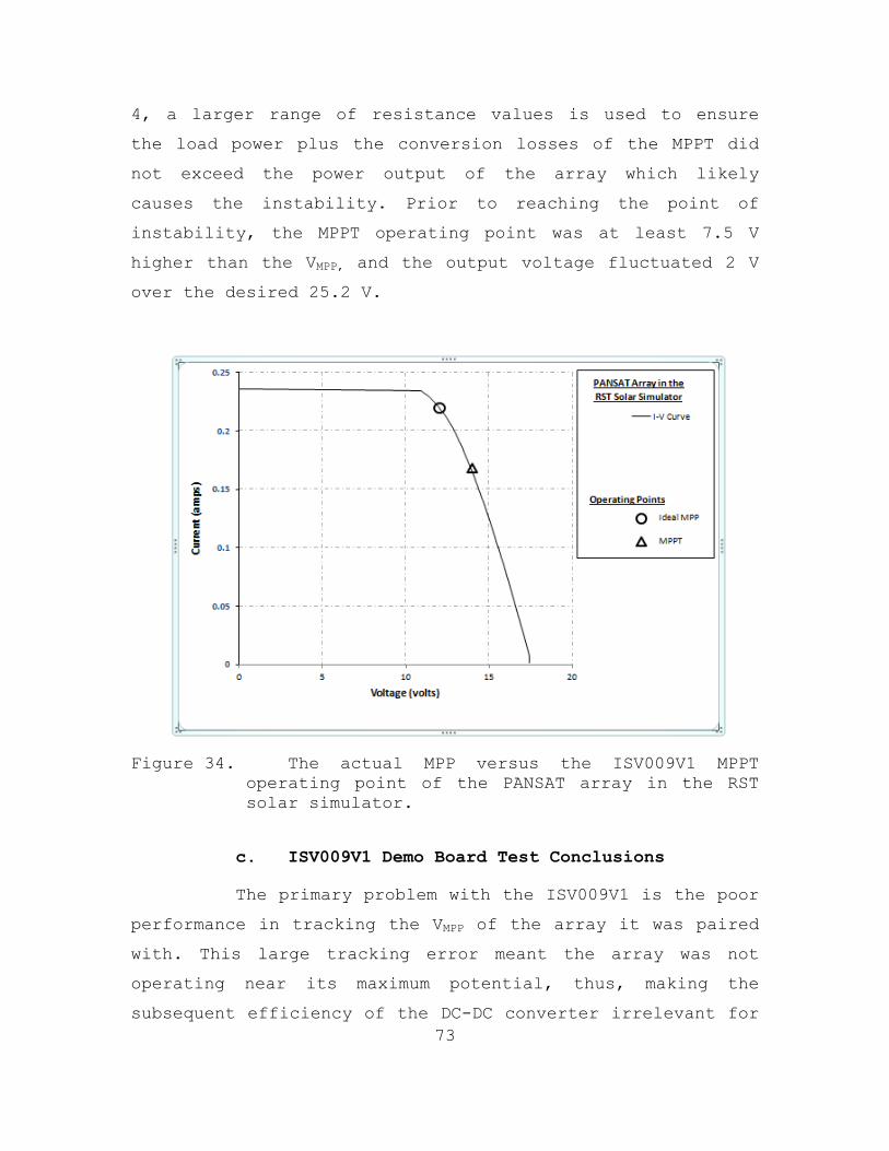
73

4, a larger range of resistance values is used to ensure

the load power plus the conversion losses of the MPPT did

not exceed the power output of the array which likely

causes the instability. Prior to reaching the point of

instability, the MPPT operating point was at least 7.5 V

higher than the VMPP, and the output voltage fluctuated 2 V

over the desired 25.2 V.

Figure 34. The actual MPP versus the ISV009V1 MPPT

operating point of the PANSAT array in the RST solar simulator.

c. ISV009V1 Demo Board Test Conclusions

The primary problem with the ISV009V1 is the poor

performance in tracking the VMPP of the array it was paired

with. This large tracking error meant the array was not

operating near its maximum potential, thus, making the

subsequent efficiency of the DC-DC converter irrelevant for

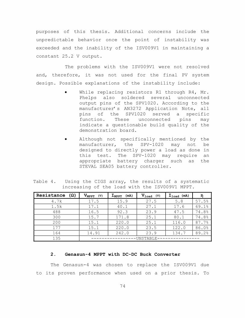
74

purposes of this thesis. Additional concerns include the

unpredictable behavior once the point of instability was

exceeded and the inability of the ISV009V1 in maintaining a

constant 25.2 V output.

The problems with the ISV009V1 were not resolved

and, therefore, it was not used for the final PV system

design. Possible explanations of the instability include:

While replacing resistors R1 through R4, Mr. Phelps also soldered several unconnected output pins of the SPV1020. According to the manufacturer’s AN3272 Application Note, all pins of the SPV1020 served a specific function. These unconnected pins may indicate a questionable build quality of the demonstration board.

Although not specifically mentioned by the manufacturer, the SPV-1020 may not be designed to directly power a load as done in this test. The SPV-1020 may require an appropriate battery charger such as the STEVAL SEA05 battery controller.

Table 4. Using the CIGS array, the results of a systematic increasing of the load with the ISV009V1 MPPT.

Resistance (Ω) VMPPT (V) IMPPT (mA) Vload (V) Iload (mA) η4.7k 17.5 15.9 27.5 5.8 57.5%1.5k 17.1 40.1 27.1 17.6 69.1%488 16.5 92.3 23.9 47.5 74.8%300 15.7 171.8 25.1 80.1 74.8%200 15.1 220.0 25.1 116.0 87.7%177 15.1 220.0 23.5 122.0 86.0%164 14.91 242.0 23.9 134.7 89.2%135 -----------------UNSTABLE----------------

2. Genasun-4 MPPT with DC-DC Buck Converter

The Genasun-4 was chosen to replace the ISV009V1 due

to its proven performance when used on a prior thesis. To

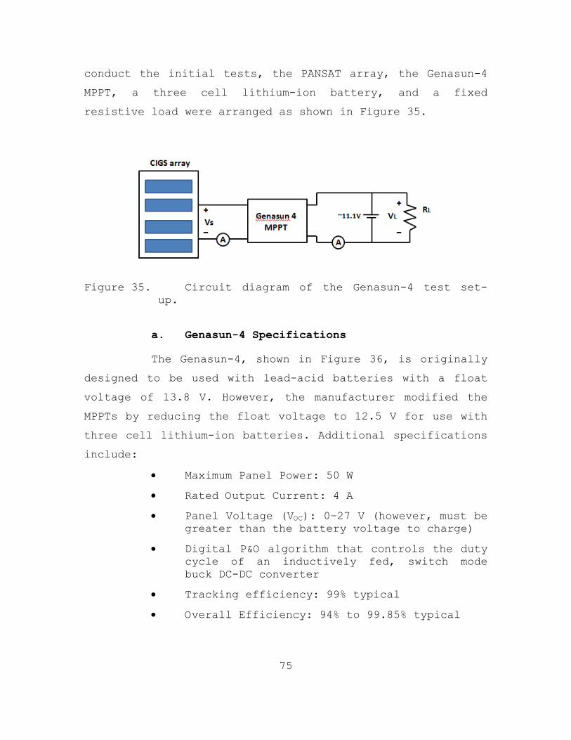
75

conduct the initial tests, the PANSAT array, the Genasun-4

MPPT, a three cell lithium-ion battery, and a fixed

resistive load were arranged as shown in Figure 35.

Figure 35. Circuit diagram of the Genasun-4 test set-

up.

a. Genasun-4 Specifications

The Genasun-4, shown in Figure 36, is originally

designed to be used with lead-acid batteries with a float

voltage of 13.8 V. However, the manufacturer modified the

MPPTs by reducing the float voltage to 12.5 V for use with

three cell lithium-ion batteries. Additional specifications

include:

Maximum Panel Power: 50 W

Rated Output Current: 4 A

Panel Voltage (VOC): 0–27 V (however, must be greater than the battery voltage to charge)

Digital P&O algorithm that controls the duty cycle of an inductively fed, switch mode buck DC-DC converter

Tracking efficiency: 99% typical

Overall Efficiency: 94% to 99.85% typical

76

Figure 36. The Genasun-4 MPPT with DC-DC buck converter

and charge controller.

b. Genasun-4 Testing

The Genasun-4 was paired with a CIGS array and

tested outdoors. Full irradiance and two degradations of

irradiance were tested by shading six of the 48 cells

within the array as shown in Figure 37. The effects of

temperature were reasonably controlled by allowing the

array to reach a relatively constant temperature of 105 F.

The goal of testing was to verify the effectiveness of the

P&O algorithm and calculate the MPPT’s efficiency.

Figure 37. The methods used to simulate partial and

severe shading of the CIGS array.

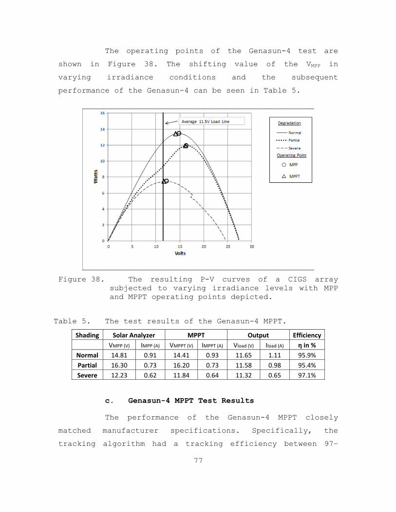
77

The operating points of the Genasun-4 test are

shown in Figure 38. The shifting value of the VMPP in

varying irradiance conditions and the subsequent

performance of the Genasun-4 can be seen in Table 5.

Figure 38. The resulting P-V curves of a CIGS array

subjected to varying irradiance levels with MPP and MPPT operating points depicted.

Table 5. The test results of the Genasun-4 MPPT.

Shading Solar Analyzer MPPT Output Efficiency

VMPP (V) IMPP (A) VMPPT (V) IMPPT (A) Vload (V) Iload (A) η in %

Normal 14.81 0.91 14.41 0.93 11.65 1.11 95.9%

Partial 16.30 0.73 16.20 0.73 11.58 0.98 95.4%

Severe 12.23 0.62 11.84 0.64 11.32 0.65 97.1%

c. Genasun-4 MPPT Test Results

The performance of the Genasun-4 MPPT closely

matched manufacturer specifications. Specifically, the

tracking algorithm had a tracking efficiency between 97–

78

99%. The total conversion efficiency (i.e., the tracking

error and DC-DC conversion losses are subtracted) ranged

between 95–97%. The load voltage averaged 11.52 V with

fluctuations less than 0.2 V. Due to the accuracy of the

MPPT algorithm and the high overall system efficiency, the

Genasun-4 was selected for use in the final system design.

C. SOLAR PANEL SELECTION

The selection of the two solar panels was primarily

influenced by the Genasun-4 MPPT specifications. The array

requirements that must be satisfied include:

VOC cannot exceed 27 V.

The power of all panels combined cannot exceed 50 W.

The charging voltage must always exceed the battery voltage.

The first panel that met most of the requirements was

the PANSAT panel. However, during the ISV00091 MPPT

testing, we discovered that the PANSAT panel has a VMPP of

11.97 V as depicted in Figure 34. This was determined to be

a problem since the test plan called for significantly

degrading the irradiance levels which causes the VMPP to

drop. Since the battery voltage range is between 8.1 to

12.5 V, the MPPT algorithm will not track the MPP once the

VMPP of the array drops below the battery voltage. To ensure

the VMPP would always exceed the battery float voltage of

12.5 V, a DC voltage source of 5.0 V was placed in series

with the PANSAT panel, and new VMPP of 16.97 V was obtained.

This technique maintains the shape of the characteristic I-

V curve with the exception of shifting it to the right by

5.0 V.

79

The second panel that was used for testing included

two strings of the degraded CIGS array (i.e., 32 cells in

series). Only two strings were selected to prevent the VOC

of the CIGS array from exceeding the Genasun’s maximum

input voltage of 27 V. The CIGS panel had a VMPP of 6.6 V,

which is well below the battery voltage range. Thus, for

similar VMPP concerns previously mentioned with the PANSAT

panel, a DC voltage source of 9.8 V was placed in series

with the CIGS panel to give a new VMPP of approximately 16.4

V.

D. FINAL DESIGN

The final design of the solar panels and MPPTs

supported three test scenarios. First, the panels would be

tested in the direct loading approach as shown in Figure

39.

Figure 39. Circuit schematic for the direct loading

approach.

80

Then, the central converter approach would be tested

as shown in Figure 40.

Figure 40. The circuit schematic for the central

converter approach.

Finally, the micro-converter approach would be tested

as shown in Figure 41.

Figure 41. The circuit schematic for the micro-

converter approach.

81

An image of the actual equipment used is shown in

Figure 42.

Figure 42. The primary equipment used to conduct the

tests.

E. DATA

Varying the levels of irradiance was accomplished by

independently tilting the arrays at approximated angles

from the sun. For example, the 0°/30° position means the

CIGS wing was normal to the sun, and the PANSAT was offset

by approximately 30 degrees. For each position, the three

test scenarios were implemented, and the relevant voltage

and current values were recorded. The I-V curves for each

array configuration and the operating points of the direct

loading, central converter, and micro-converter tests are

graphically depicted in Appendix C. Although the individual

test data points in Appendix C and the following tables are

relevant, a summary of the power delivered to the loads and

MPPT efficiency is shown in Table 10 and can be used as the

primary reference when drawing conclusions.

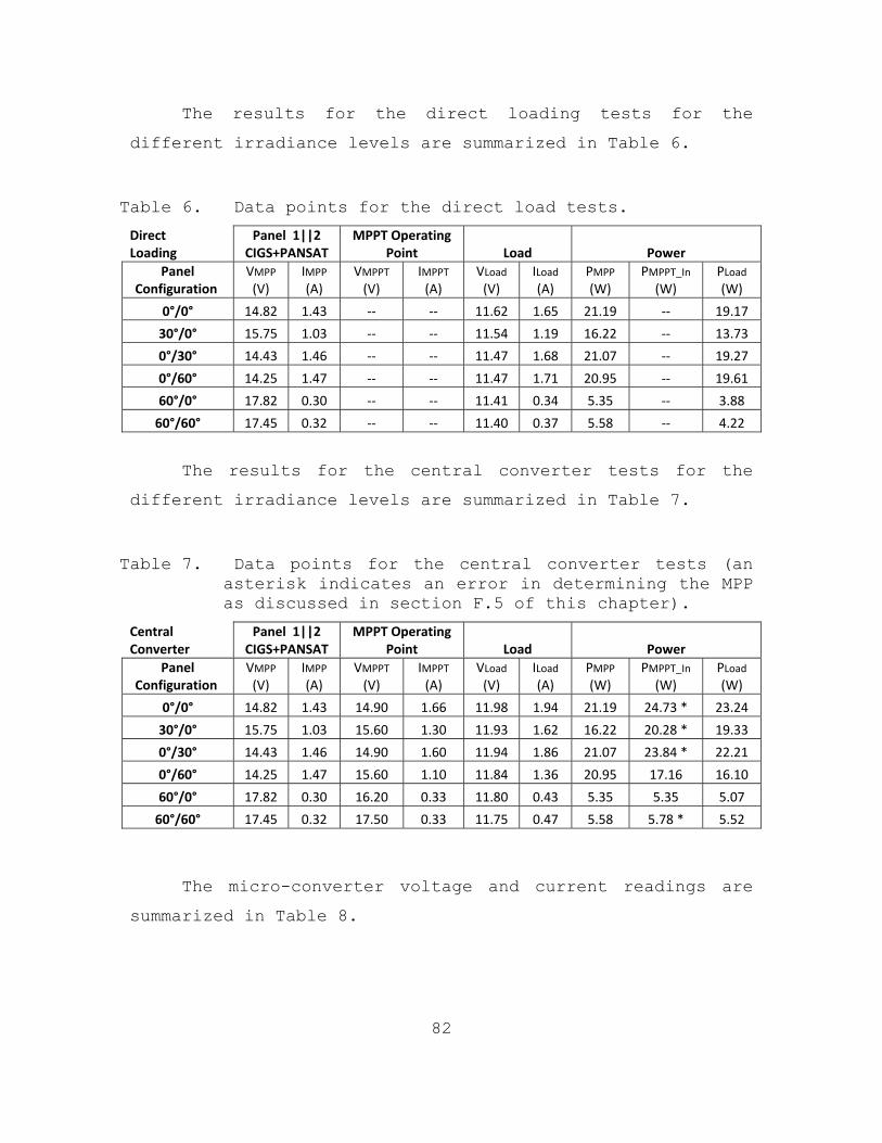
82

The results for the direct loading tests for the

different irradiance levels are summarized in Table 6.

Table 6. Data points for the direct load tests.

Direct Loading

Panel 1||2 CIGS+PANSAT

MPPT Operating Point Load Power

Panel Configuration

VMPP (V)

IMPP (A)

VMPPT

(V) IMPPT

(A) VLoad(V)

ILoad(A)

PMPP

(W) PMPPT_In

(W) PLoad (W)

0°/0° 14.82 1.43 ‐‐ ‐‐ 11.62 1.65 21.19 ‐‐ 19.17

30°/0° 15.75 1.03 ‐‐ ‐‐ 11.54 1.19 16.22 ‐‐ 13.73

0°/30° 14.43 1.46 ‐‐ ‐‐ 11.47 1.68 21.07 ‐‐ 19.27

0°/60° 14.25 1.47 ‐‐ ‐‐ 11.47 1.71 20.95 ‐‐ 19.61

60°/0° 17.82 0.30 ‐‐ ‐‐ 11.41 0.34 5.35 ‐‐ 3.88

60°/60° 17.45 0.32 ‐‐ ‐‐ 11.40 0.37 5.58 ‐‐ 4.22

The results for the central converter tests for the

different irradiance levels are summarized in Table 7.

Table 7. Data points for the central converter tests (an asterisk indicates an error in determining the MPP as discussed in section F.5 of this chapter).

Central Converter

Panel 1||2 CIGS+PANSAT

MPPT Operating Point Load Power

Panel Configuration

VMPP (V)

IMPP (A)

VMPPT

(V) IMPPT

(A) VLoad(V)

ILoad(A)

PMPP

(W) PMPPT_In

(W) PLoad (W)

0°/0° 14.82 1.43 14.90 1.66 11.98 1.94 21.19 24.73 * 23.24

30°/0° 15.75 1.03 15.60 1.30 11.93 1.62 16.22 20.28 * 19.33

0°/30° 14.43 1.46 14.90 1.60 11.94 1.86 21.07 23.84 * 22.21

0°/60° 14.25 1.47 15.60 1.10 11.84 1.36 20.95 17.16 16.10

60°/0° 17.82 0.30 16.20 0.33 11.80 0.43 5.35 5.35 5.07

60°/60° 17.45 0.32 17.50 0.33 11.75 0.47 5.58 5.78 * 5.52

The micro-converter voltage and current readings are

summarized in Table 8.

83

Table 8. Voltage and current readings for the micro-converter tests (an asterisk indicates a “bypass” mode as discussed in Section F.4 of this chapter).

Micro‐converter

MPP Panel 1 (CIGS)

MPPT 1 Operating Point Load 1

MPP Panel 2 (PANSAT)

MPPT 2 Operating Point Load 2

Panel Configuration

VMPP

(V)

IMPP (A)

VMPPT (V)

IMPPT

(A)

VLoad

(V)

ILoad

(A)

VMPP

(V)

IMPP

(A)

VMPPT

(V) IMPPT (A) VLoad (V) ILoad (A)

0°/0° 15.15 1.34 14.75 1.33 11.9 1.58 16.44 0.25 16.56 0.24 11.9 0.31

30°/0° 16.27 0.97 16.00 0.98 11.90 1.25 16.44 0.25 16.47 0.24 11.9 0.31

0°/30° 15.15 1.34 14.9 1.36 11.83 1.58 17.24 0.17 17.30 0.17 11.8 0.21

0°/60° 15.15 1.34 15.2 1.37 11.84 1.63 17.26 0.03 11.8* 0.04 11.8 0.04

60°/0° 18.24 0.32 17.9 0.31 11.74 0.44 16.08 0.24 15.93 0.24 11.7 0.30

60°/60° 18.24 0.32 17.9 0.32 11.70 0.46 17.26 0.03 11.7* 0.04 11.7 0.04

The micro-converter power calculations are contained in

Table 9.

Table 9. Power calculations for the micro-converter tests.

Micro‐converter Power

Panel Configuration PMPP (W) PMPPT_In (W) PLoad (W)

0°/0° 24.33 23.61 22.54

30°/0° 19.81 19.70 18.61

0°/30° 23.25 23.21 21.18

0°/60° 20.89 21.27 19.73

60°/0° 9.75 9.37 8.69

60°/60° 6.46 6.16 5.80

84

Table 10. A power and overall system efficiency analysis for the three test scenarios (an asterisk indicates an MPP tracking error as discussed in Section F.5 of this chapter).

Power Delivered/Overall Efficiency Power (W) / (Efficiency %)

Panel Configuration Direct Loading Central Converter Micro‐inverter

0°/0° 19.17 / (n/a) 23.24 / (94 % *) 22.54 / (93%)

30°/0° 13.73 / (n/a) 19.33 / (95% *) 18.61 / (94%)

0°/30° 19.27 / (n/a) 22.21 / (93% *) 21.18 / (91%)

0°/60° 19.61 / (n/a) 16.10 / (94% ) 19.73 / (94%)

60°/0° 3.88 / (n/a) 5.07 / (95%) 8.69 / (89%)

60°/60° 4.22 / (n/a) 5.52 / (99 % *) 5.80 / (90%)

F. OBSERVATIONS

1. MPPTs Outperform the Direct Loading Approach

As shown in Table 10, the power delivered to the load

when using either one or two MPPTs almost always exceeded

the direct loading method. The one abnormality occurred in

the 0⁰/60⁰ test between the direct loading and central

converter methods. Possible explanations include operator

error or equipment malfunction.

2. Micro-inverters Versus Central Converter

The primary advantage of using micro-inverters vice a

central converter is apparent when the arrays encountered

extreme differences in the levels of irradiance. This

observation can be seen by referring to Table 10 and

comparing the power delivered when the difference in

irradiance levels was relatively similar (i.e., 30⁰ or less)

and when they were drastically different (i.e., 60⁰ between

arrays). The micro-converter approach delivered

significantly more power than the central converter method

in both the 0⁰/60⁰ and 60⁰/0⁰ tests. However, when the micro-

85

converter method is compared to direct loading in the 0⁰/60⁰

test, the minor gain in power delivered would appear to

contradict this observation. This incongruity is a result

or a more linear I-V curve that is caused by using a

degraded CIGS array. The relationship between an array’s FF

and the use of MPPTs is discussed further in the final

chapter.

A disadvantage to using micro-inverters versus a

central converter can be seen in Table 10 by comparing the

power delivered when the arrays experienced similar

irradiance conditions. In the 0°/0°, 30°/0°, and the 0°/30°

configurations, the power delivered to the load was

significantly less than the central converter method.

3. Tracking Accuracy

The P&O algorithm took approximately five seconds to

transition from VOC operating point to its self-calculated

VMPPT. When calculating the tracking accuracy, the two severe

degradations of the PANSAT panel (i.e., the 0°/60° and

60°/60° configurations) in the micro-converter tests were

omitted due to a “bypass” mode being triggered by the

Genasun-4. Excluding those two test points, the Genasun-4

averaged a 98% tracking accuracy.

4. Bypass Mode

The bypass mode can be identified when the Genasun’s

input operating points mirror the load voltage and current.

In other words, the MPPT appears to recognize when certain

design limitations have been reached and allows array

output power to be directly delivered to the load by

passing through the MPPT. This mode is indicated by the use

86

of asterisks in Table 8. The pass-through mode can be

identified by comparing the voltage and current values when

the PANSAT array is severely degraded (i.e., the 60⁰

position). These two specific scenarios appear to activate

the bypass mode for different reasons. The first scenario

is when the current level is such a small value that

perturbations in the operating point yield no measurable

gain or loss in the array’s power. This would mean the P&O

tracking algorithm has difficulty in locating the VMPP due

to a flattened P-V curve. In the second scenario, the MPPT

activates the bypass mode when the VMPP drops below the

charging voltage. As stated in the product specifications,

the array voltage must be higher than the battery voltage

in order to charge.

While the bypass mode may not be as significant to

some applications, this design feature increased the power

delivered to the load by approximately 2.5% in these two

scenarios. The manufacturer’s decision to include a bypass

mode vice shutting down the MPPT when certain design

limitations have been exceeded is a desirable attribute. On

a side note, the manufacturer does not specifically mention

this mode of operation, thus, the term “bypass” is used for

lack of a more proper term.

5. MPP error during central converter test

As shown by the use of asterisks in Table 7 during the

central converter tests, the MPPT operating point during

four of the six irradiance configurations resulted in a

power calculation that far exceeded the MPP as measured by

the Solar-600 analyzer. The central converter tests were

the only time during testing the MPPT produced more power

87

than the Solar-600 analyzer’s estimation of the actual MPP.

Reasons for this error are not understood.

88


89

VI. CONCLUSIONS

The PV system designer has many options available if

they choose to build their own MPPT. However, the decision

to utilize a commercially available MPPT will most likely

result in a digital microprocessor with a P&O or slightly

modified P&O algorithm. These commercial P&O MPPTs are

efficient, reliable, and becoming extremely affordable.

However, their primary disadvantage resides in the P&O

tracking algorithm. Depending on how far the MPP shifts due

to changing environmental conditions, the P&O algorithm can

take up to 2.6 seconds or longer to successfully change the

array’s operating point to the new MPP. It is this author’s

opinion that the digital P&O MPPTs currently available in

the commercial market will successfully meet the

performance specifications of most Department of Defense

(DoD) solar applications. A slight increase in expense

might be encountered in order to meet the reliability and

durability requirements of the military. However, the

dynamic environment that the military operates is where

this research has concluded the multiple MPPT approach

works best and a slight expense may be worthwhile.

For specialized applications that require a faster

tracking response time (i.e., a rotating satellite), the PV

system designer should consider more advanced algorithms

such as fuzzy logic and neural networks. While not

discussed in depth in this research, these advanced

algorithms can learn from past behavior and are able to

effectively respond to nonlinear inputs such as rapidly

changing environmental conditions. However, these advanced

90

algorithms require more processing power to implement and

are cost prohibitive for most commercial applications.

Finally, the emergence of efficient analog MPPT

algorithms combined with the promising research into

capacitively fed, switch-mode converter technologies

presents the best option for realizing the ideal, per cell

application of MPPTs. This distributed PV architecture

would be extremely beneficial as each cell could be

optimized to perform at the MPP despite manufacturing

irregularities, local environmental degradations, or cell

damage.

The remaining sections in this chapter are a summary

of primary conclusions that resulted from this research and

recommendations are made for future work.

A. CONCLUSIONS

1. MPPT Versus Direct-Loading

The results showed that in every test configuration,

the central converter and micro-converter approach

outperformed direct loading. Although this conclusion might

be considered predictable due to numerous academic studies

and a successful MPPT commercial market, the author found

that DoD solar applications typically rely on direct-

loading vice using MPPTs. The reason behind this has its

advantages; a well-designed, directly-loaded PV system will

have a MPP near or slightly above the load voltage. This

results in a simple, reliable, and for most applications, a

cost-effective PV system. However, as validated in this

research, a slight shift in the MPP due to environmental

conditions has a substantial effect on the power output of

91

the array. With consideration to the reliability and

affordability of modern MPPTs, there should be at a minimum

of one MPPT per PV system for DoD applications that are

subjected to dynamic operating conditions (i.e., solar

blankets or UAVs).

2. Multiple MPPT Performance

The multiple MPPT approach provided the most benefit

when the two panels experienced drastically different

irradiance levels (i.e, 60⁰ of tilt). This research mirrored

the advertised claims of the micro-inverter manufacturers.

In particular, it was seen that localized disruptions

disproportionately affect the output power of the entire

array. However, it was also noticed that the micro-

converter approach was on par with the central converter

configuration when the PV system experienced slight

variations of irradiance (i.e., 30⁰ or less). Thus, the term

“localized disruption” is ambiguous, and the factors that

determine at which point the micro-converter approach

outperforms the central converter configuration was not

resolved with this research.

3. FF Versus MPPT Performance

Arrays with a poor FF are not a great candidate for

MPPTs. This conclusion was first noticed when analyzing the

results from the initial Genasun-4 MPPT testing. According

to the Solar-600 analyzer, the degraded CIGS array had a

very low fill factor (i.e., approximately 38%). Due to the

linear I-V curve that results from a poor FF, changes in

the operating point yield nominal increases or decreases in

power. This can be graphically depicted in Figure 43 where

92

the I-V curves of a degraded CIGS array, a newer CIGS

array, and a traditional silicone array is compared. It can

be seen that for the same 3.0 V shift towards the MPP that

is applied to both the degraded CIGS (i.e., point A to B)

and the silicon panel (i.e., point C to D), a drastically

different power output is achieved. This can be seen

graphically by comparing the size of the rectangles that

exist between the two operating points for each I-V curve.

The power represented by the rectangles at point A and B

are approximately equal in size. Thus, due to the linear I-

V curve caused by the poor FF of the degraded CIGS array,

shifting the operating point only yielded a gain of 12%.

However, the same 3.0 V shift with the silicon array yields

a significant increase (i.e., approximately 50%) in power

as graphically depicted by the larger rectangle created by

operating at point D vice point C.

Common explanations for a poor FF include inferior

quality, degradation due to age, or cell damage. Regardless

of the reason, this research has concluded that cells with

a poor FF will see at best, a slight increase in output

power when paired with one or multiple MPPTs. In

particularly low FF arrays (i.e., less than 40%), the

increase was relatively insignificant.

B. RECOMMENDATIONS FOR FUTURE WORK

1. A More Refined Method in Validating the Nultiple MPPT Approach

The ability to precisely control the changes in

environmental conditions would provide for a more accurate

performance characterization for all three test

configurations (i.e., direct-loading, central-converter,

93

and micro-converter). Recommendations include modeling the

system and/or ensuring the PV panels utilized can fit

inside the solar simulator. Additionally, a more

sophisticated PV system that is comprised of more than two

panels could provide further insight into how the system

behaves when exposed to a wider range of environmental

conditions.

2. Design of a “Per Cell” MPPT

With the recent advances in tracking algorithms that

require relatively few parts (i.e., analog TEODI or small

microprocessors) combined with highly efficient and

increasingly smaller converters, an MPPT could be designed

to be applied to each individual cell within an array. This

research would be challenging due to the lack of space

available on solar arrays. However, the recent advancements

in MPPT technology has made this concept worth further

investigation.

3. Capacitor-Based Converter Technologies

Relatively heavy, switch-mode converters are used in

almost all portable electronics. Research into a lighter

and smaller technology that replaces inductively fed

converters would have benefits that extend well beyond

MPPTs.

94

Figure 43. A visual representation of how a poor FF

adversely affects MPPT performance.

Point A to B yields +0.20 W

A

B

C

D

Point C to D yields +1.40 W

MPP

MPP

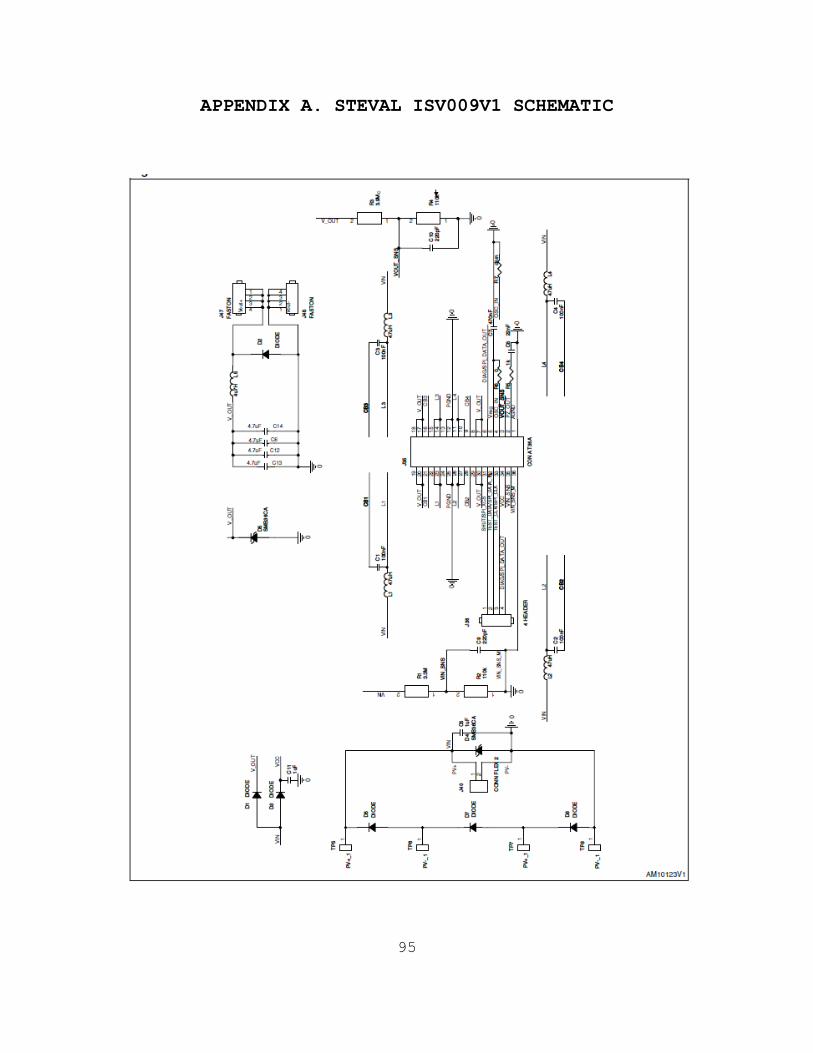
95

APPENDIX A. STEVAL ISV009V1 SCHEMATIC

96


97

APPENDIX B. AMPROBE SOLAR-600 ANALYSIS EXAMPLE

Sample No. 48

PANSAT Silicon

Date & Time ‐‐

Vopen (V) 19.43

Ishort (A) 0.265

Vmaxp (V) 13.54

Imaxp (A) 0.247

Pmax (W) 3.357

V (V) I (A) P (W)

19.454 0.0016 0.031126

19.45 0.0034 0.06613

19.447 0.0052 0.101124

19.446 0.007 0.136122

19.417 0.0088 0.17087

19.382 0.0106 0.205449

19.348 0.0122 0.236046

19.315 0.014 0.27041

19.275 0.0158 0.304545

19.241 0.0176 0.338642

19.206 0.0194 0.372596

19.174 0.0212 0.406489

19.136 0.023 0.440128

19.106 0.0246 0.470008

19.07 0.0264 0.503448

19.037 0.0282 0.536843

18.999 0.03 0.56997

18.966 0.0318 0.603119

18.933 0.0336 0.636149

18.902 0.0354 0.669131

18.868 0.037 0.698116

18.835 0.0388 0.730798

18.802 0.0406 0.763361

18.768 0.0424 0.795763

18.736 0.0442 0.828131

18.698 0.046 0.860108

V (V) I (A) P (W)

18.665 0.0478 0.892187

18.631 0.0494 0.920371

18.597 0.0512 0.952166

18.563 0.053 0.983839

18.53 0.0548 1.015444

18.497 0.0566 1.04693

18.462 0.0584 1.078181

18.424 0.0602 1.109125

18.389 0.0618 1.13644

18.359 0.0636 1.167632

18.326 0.0654 1.19852

18.295 0.0672 1.229424

18.261 0.069 1.260009

18.228 0.0708 1.290542

18.194 0.0724 1.317246

18.161 0.0742 1.347546

18.123 0.076 1.377348

18.087 0.0778 1.407169

18.046 0.0796 1.436462

18.01 0.0814 1.466014

17.972 0.0832 1.49527

17.938 0.0848 1.521142

17.902 0.0866 1.550313

17.866 0.0884 1.579354

17.828 0.0902 1.608086

17.794 0.092 1.637048

17.758 0.0938 1.6657

17.723 0.0956 1.694319

17.684 0.0972 1.718885

17.648 0.099 1.747152

17.612 0.1008 1.77529

17.578 0.1026 1.803503

17.539 0.1044 1.831072

17.504 0.1062 1.858925

17.468 0.108 1.886544

17.434 0.1096 1.910766

V (V) I (A) P (W)

17.395 0.1114 1.937803

17.358 0.1132 1.964926

17.322 0.115 1.99203

17.284 0.1168 2.018771

17.244 0.1186 2.045138

17.207 0.1204 2.071723

17.169 0.122 2.094618

17.134 0.1238 2.121189

17.092 0.1256 2.146755

17.059 0.1274 2.173317

17.021 0.1292 2.199113

16.985 0.131 2.225035

16.942 0.1328 2.249898

16.904 0.1344 2.271898

16.862 0.1362 2.296604

16.824 0.138 2.321712

16.786 0.1398 2.346683

16.746 0.1416 2.371234

16.707 0.1434 2.395784

16.669 0.145 2.417005

16.627 0.1468 2.440844

16.588 0.1486 2.464977

16.548 0.1504 2.488819

16.509 0.1522 2.51267

16.472 0.154 2.536688

16.428 0.1558 2.559482

16.39 0.1574 2.579786

16.347 0.1592 2.602442

16.308 0.161 2.625588

16.264 0.1628 2.647779

16.223 0.1646 2.670306

16.181 0.1664 2.692518

16.138 0.1682 2.714412

16.096 0.1698 2.733101

16.05 0.1716 2.75418

16.008 0.1734 2.775787

98

V (V) I (A) P (W)

15.966 0.1752 2.797243

15.919 0.177 2.817663

15.877 0.1788 2.838808

15.833 0.1806 2.85944

15.788 0.1822 2.876574

15.739 0.184 2.895976

15.684 0.1858 2.914087

15.638 0.1876 2.933689

15.595 0.1894 2.953693

15.551 0.1912 2.973351

15.504 0.193 2.992272

15.459 0.1946 3.008321

15.412 0.1964 3.026917

15.364 0.1982 3.045145

15.314 0.2 3.0628

15.262 0.2018 3.079872

15.212 0.2036 3.097163

15.163 0.2052 3.111448

V (V) I (A) P (W)

15.11 0.207 3.12777

15.055 0.2088 3.143484

15.035 0.2106 3.166371

14.985 0.2124 3.182814

14.928 0.2142 3.197578

14.867 0.216 3.211272

14.81 0.2176 3.222656

14.748 0.2194 3.235711

14.687 0.2212 3.248764

14.618 0.223 3.259814

14.555 0.2248 3.271964

14.49 0.2266 3.283434

14.422 0.2284 3.293985

14.356 0.23 3.30188

14.284 0.2318 3.311031

14.212 0.2336 3.319923

14.149 0.2354 3.330675

14.075 0.2372 3.33859

V (V) I (A) P (W)

13.988 0.239 3.343132

13.902 0.2408 3.347602

13.823 0.2424 3.350695

13.736 0.2442 3.354331

13.64 0.246 3.35544

13.548 0.2478 3.357194

13.428 0.2496 3.351629

13.325 0.2514 3.349905

13.212 0.2532 3.345278

13.095 0.2548 3.336606

12.955 0.2566 3.324253

12.815 0.2584 3.311396

12.672 0.2602 3.297254

12.48 0.262 3.26976

12.241 0.2638 3.229176

0 0.2656 0

99

APPENDIX C. TEST RESULTS

The following figures are a graphical representation

of the data obtained by the Solar-600 analyzer for the

three different test configurations under varying levels of

irradiance. The results for the 0°/0° irradiance level are

shown in Figure 44. The results for the 30°/0° irradiance

level are shown in Figure 45. The results for the 0°/30°

irradiance level are shown in Figure 46. The results for

the 0°/60° irradiance level are shown in Figure 47. The

results for the 60°/0° irradiance level are shown in Figure

48. The results for the 60°/60° irradiance level are shown

in Figure 49.

Figure 44. The I-V curves and operating points for

irradiance level 0°/0°.

100





101





102


irradiation level 60°/60°.

103

LIST OF REFERENCES

[1] B. Betz. (2012, September 5). PV microinverters and power optimizers set for significant growth [PV Magazine Online]. Available: http://www.pv-magazine.com/news/details/beitrag/pv-microinverters-and-power-optimizers-set-for-significant-growth_100008296/#axzz26lVQcSs7

[2] D. Hettelsater, et al. (2002, May 2). Lab 7: solar

cells [Online]. Available: http://classes.soe.ucsc.edu/ee145/Spring02/EE145Lab7.pdf

[3] A. D. Gleue. (2008, June). The basics of a

photovoltaic solar cell [Online]. Available: http://teachers.usd497.org/agleue/Gratzel_solar_cell%20assets/Basics%20of%20a%20Photovoltaic%20%20Solar%20Cell.htm

[4] R. M. Fernadez, Jr., “A novel photovoltaic power

converter for military and space applications,” M.S. thesis, Dept. Electron. Eng., Naval Postgraduate School, Monterey, California, 2005.

[5] Solar Electricity Handbook: Solar Irradiance.

Greenstream Publishing, Warwickshire, United Kingdom, 2009 [Online]. Available: http://solarelectricityhandbook.com/solar-irradiance.html

[6] G. Kopp and J. Lean. (2011, January 14). “A new, lower

value of total solar irradiance: evidence and climate significance,” in Geophysical Research Letters [Online], vol. 38, L01706. Available: http://www.agu.org/pubs/crossref/2011/2010GL045777.shtml

[7] S. Michael, “Solar cell basics notes for EC3230 (Space

Power and Radiation Effects),” unpublished, Naval Postgraduate School, Monterey, California.

[8] M. Berrera et al., “Experimental test of seven widely-

adopted MPPT algorithms,” in IEEE Power Tech Conf., Budapest, Hungary, 2009.

104

[9] J.Jiang et al., “Maximum power point tracking for PV power systems,” in Tamkang Journal of Science and Engineering, Vol. 8, No. 2, 2005 pp. 147–153.

[10] D. P. Hohm and M. E. Ropp, “Comparative study of

maximum power point tracking algorithms,” in Progress in Photovoltaics: Research and Applications, Vol. 11, Issue 1, 2003, pp. 47–62.

[11] J. Ahmad, “A fractional open circuit voltage based

MPPT for PV arrays,” in IEEE 2nd Int. Conf. on Software Technology and Engineering, Ansan, South Korea, 2010.

[12] D. Petreus et al., “A novel implementation of a

maximum power point tracking system with digital control,” in IEEE Int. Sym. on Industrial Electronics, Cluj-Napoca, Romania, 2011.

[13] Y. Jiang et al., “Load current based analog MPPT

controller for PV systems,” in 27th Annual Applied Power Electronics Conf. and Expo., Tuscaloosa, AL, 2012.

[14] N. Femia et al., “A new analog MPPT technique: TEODI,”

in IEEE Progress in Photovoltaics: Research and Applications, Vol. 18, 2010, pp.28–41.

[15] S. Kim and G. Rincon-Mora, “Efficiency of switched-

inductor dc-dc converter ICs across process technologies,” in IEEE Explore, 2012 [Online]. Available: http://ieeexplore.ieee.org/stamp/stamp.jsp?arnumber=06272064

[16] S. Keeping. (2012, July). Techniques to limit

switching dc/dc converter inefficiency during low loads [Electronic Products Online]. Available: http://www.digikey.com/us/en/techzone/power/resources/articles/techniques-to-limit-switching-dc-dc-inefficiency.html

[17] M. Seeman et al., “A comparative analysis of switched-

capacitor and inductor-based dc-Dc conversion Technologies,” in IEEE 12th Workshop on Control and Modeling for Power Electronics, Urbana, IL, 2010.

105

[18] Wikipedia. (2012, November 8). PV microinverters [Online]. Available: http://en.wikipedia.org/wiki/Solar_micro-inverter

[19] R. Muenster. (2009, February 2). Shade happens

[National Semiconductor Online]. Available: http://www.renewableenergyworld.com/rea/news/article/2009/02/shade-happens-54551

[20] ENPHASE. (2012, November 9). Micro-inverter energy

performance analysis [Online]. Available: http://enphase.com/wp-uploads/enphase.com/2011/08/Enphase-Handout-Performance-versus-PVWatts.pdf

[21] K. Dolan, “Enphase’s rooftop solar revolution,” in

Forbes Magazine, November 2010. [22] S. Michael, “Satellite configuration notes for EC3230

(space power and radiation effects)” unpublished, Naval Postgraduate School, Monterey, California.

[23] H. Kenyon, “Off-the-shelf gear strengthens Marine

operations,” in Signal Magazine, April 2010. [24] C. Chin, “Extending the endurance, missions and

capabilities of most UAVs, using advanced flexible/ridged solar cells and using new high power density batteries technology,” M.S. thesis, Dept. Electron. Eng., Naval Postgraduate School, Monterey, California, 2011.

[25] R. Phelps, “Safe operation of RST solar simulator,

version 2,” unpublished, Space Systems Academic Group, Naval Postgraduate School, Monterey, California.

[26] Designing with the SPV1020, an interleaved boost

converter with MPPT algorithm, Steval USA, Boca Raton, FL, 2012.

106


107

INITIAL DISTRIBUTION LIST

1. Defense Technical Information Center Ft. Belvoir, Virginia 2. Dudley Knox Library Naval Postgraduate School Monterey, California 3. Marine Corps Representative Naval Postgraduate School Monterey, California 4. Professor Clark Robertson, Chairman Department of Electrical and Computer Engineering Naval Postgraduate School Monterey, California 5. Professor Sherif Michael Department of Electrical and Computer Engineering Naval Postgraduate School Monterey, California 6. Professor Robert Ashton Department of Electrical and Computer Engineering Naval Postgraduate School Monterey, California 7. Director, Training and Education, MCCDC, Code C46 Quantico, Virginia 8. Director, Marine Corps Research Center, MCCDC, Code C40RC Quantico, Virginia 9. Marine Corps Tactical Systems Support Activity (Attn: Operations Officer) Camp Pendleton, California 10. Christopher Stephenson Murfreesboro, Tennessee

Documents

Utilizing maximum power point trackers in parallel to maximize the