Embed Size (px)
Citation preview
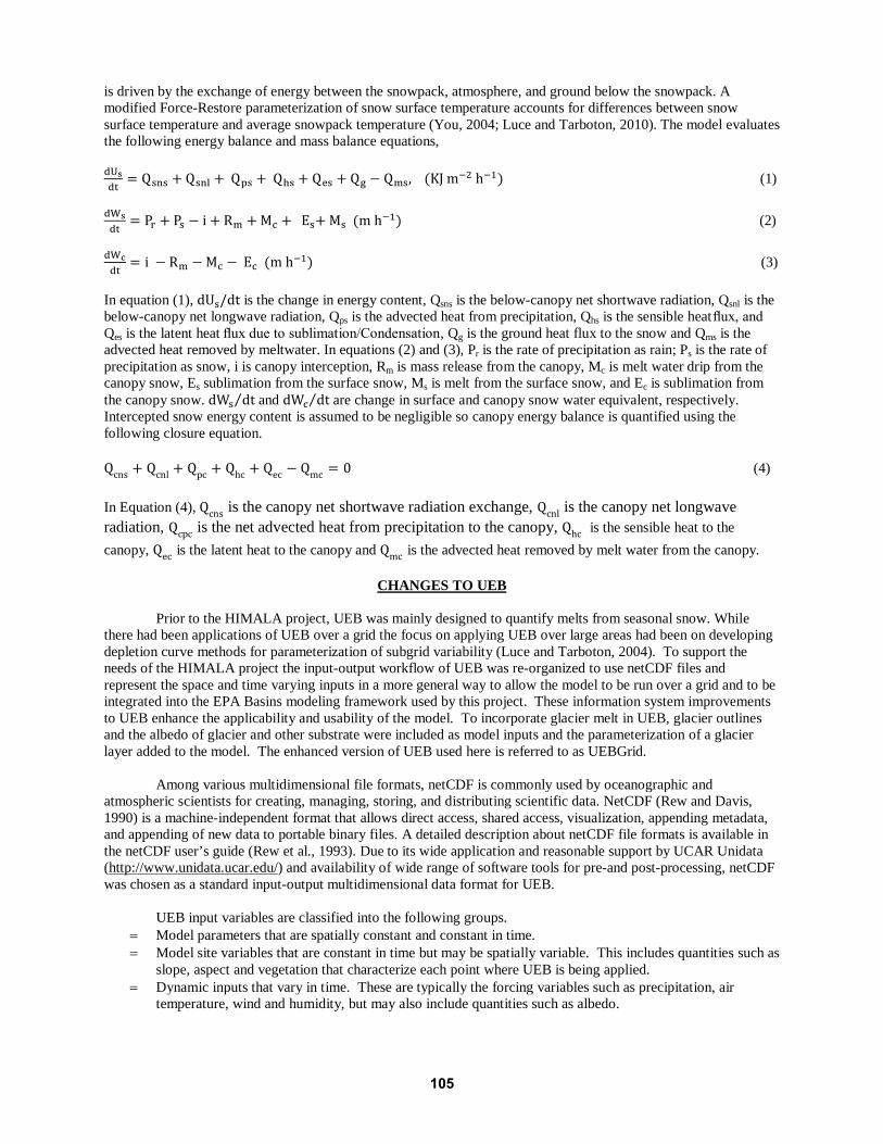
USING THE UTAH ENERGY BALANCE SNOW MELT MODEL TO QUANTIFY SNOW AND GLACIER MELT IN THE HIMALAYAN REGION
Avirup Sen Gupta1 and David G. Tarboton1
ABSTRACT
Quantification of the melting of glaciers in the Hindu-Kush Himalayan (HKH) region is important for decision making in water sensitive sectors, and for water resources management and flood protection. Access to and monitoring of the glaciers and their melt outflow is challenging, thus modeling based on remote sensing offers the potential for providing information to improve water resources decision making and management. In this paper we report on a distributed version of the Utah Energy Balance (UEB) snowmelt model, referred to as UEBGrid, which was adapted to quantify the melting of glaciers taking advantage of NASA remote sensing and earth science data products such as, satellite data, reanalysis data and climate model outputs. The representations of surface energy balance fluxes in the UEB snowmelt model have been extended to include the capability to quantify glacier melt. To account for clean and debris covered glaciers, substrate albedo determined from remote sensing, and glacier mapping is taken as an input. Representation of glaciers within the model involves inclusion of glacier ice as a substrate and generation of melt from the ice substrate when seasonal snow has melted. In UEBGrid, a watershed is divided into a mesh of grid cells and the model runs individually for each grid cell. Users have control to provide separate inputs for each grid cell, or spatially constant inputs for the entire domain. Therefore, regional variability in snow and glacier melting is computed. Outflow can be aggregated over subwatersheds defined, for example, from a digital elevation model, and input into other hydrologic models. UEBGrid was tested using weather, climate and hydrologic data at Langtang Khola Watershed, Nepal. UEBGrid is being included into the EPA BASINS software to facilitate linking to other models and to take advantage of BASINS’s capability to manage input data and visualize results. This capability for using gridded NASA Earth Science data, and the associated data model and workflow for storage and processing of data into and out of models linked in BASINS advances hydrologic information science. The capability for estimating the melt from glaciers and snow in a data sparse region will help water managers in decision making and management of water resources in areas impacted by glacier and snow melt. (KEYWORDS: glacier and snow melt, Energy balance, model, remote sensing)
INTRODUCTION
Countries in Hindu Kush-Himalayan (HKH) region are highly disaster prone and have wide variety of water resources problems. Bangladesh, for example, because of its geographical location, is affected by both seasonal droughts and floods and is vulnerable to water insecurity (Rahaman, 2002). Glaciers are headwater for many large river systems in Asia, including Ganges-Brahmaputra, Indus and Yellow rivers. Millions of people in the South Asian region depend on the fresh water generated from snow-and glacier-melting (Kehrwald et al., 2008) and are also at risk due to snow- and glacier-melt floods. South Asian countries face water insecurity due to high population and economic growth. Climate change disrupts the hydrological balance of those rivers that are mostly fed by snow and glacier melting (Barnett et al., 2005). Retreat of glaciers due to recent warming is shifting the hydrologic equilibrium and is a major social concern (Kehrwald et al., 2008). Although there is a prevalent consensus among researchers about changes in potential water sources (i.e. precipitation and glacier) due to changing climate (Vörösmarty et al., 2000); limited research has been conducted to quantify the relative contribution of these sources in discharge at watershed scale. Decision-making in water-sensitive sectors in both the short- and long-term largely depends on accurate prediction of timing and volume of discharge. The primary objective of this work is to develop a hydrological tool that includes modeling of both snow and glacier-melt water contributions to river flow in the Himalayan region. While statistics-based “lumped models” may provide satisfactory results for watershed with less hydrologic _______________________________________ Paper presented Western Snow Conference 2013 1 Avirup Sen Gupta, Utah Water Research Laboratory, Utah State University, Logan, UT. [email protected] 1 David Tarboton, Utah Water Research Laboratory, Utah State University, Logan, UT. [email protected]
103

complexity, watersheds in HKH require distributed models that capture complex topographic and hydrological phenomena and quantify the dynamic nature of water sources (Lamadrid and MacClune, 2010). However, only a limited number of studies in this region, to our best knowledge, use distributed hydrologic models, the most significant barrier to distributed modeling being data availability. Because of extreme topography and lack of financial support, in general, HKH region is not data rich. Remote sensing data has been used for various hydrological and meteorological studies such as; estimating snowmelt runoff (Thapa, 1993), characterizing glaciers (Racoviteanu et al., 2008), estimating melt and the thickness of debris-covers on glaciers. In this study, we use remote sensing data, along with reanalysis climate products and ground-based observations to model snow and glacier melt for a watershed in HKH. Our goal is to improve streamflow prediction by taking the advantage of modern remote sensing and high resolution climate data products to compensate for the scarcity of ground-based observation data. A spatially distributed version of the UEB snowmelt model (Tarboton et al., 1995; Mahat and Tarboton, 2012; Mahat et al., 2013) was enhanced as a part of the HIMALA project (Brown et al., 2010) to estimate snow- and glacier-melt and outflow on grid distributed over a watershed. The model enhancements retained the process physics of the previous version of UEB and added a new approach to represent glacier as a substrate layer and compute melt from glacier substrate when seasonal snow has melted. Glacier outlines and albedo of snow, glacier and debris covered glaciers are used as input to the model. The distribution of snow and its temporal-spatial pattern has been of great interest in the scientific community. The development of remote sensing technologies, especially after the launching of MODIS at the end of 1999, has enabled our ability to continuously monitor snow-cover (Hall et al., 2002). Using remote sensing images, the extent of the snow covered area can be measured; however, remote sensing is not able to measure the depth of snow. On the other hand, Snow water equivalent (SWE) is one of the many outputs of the UEB model. UEB estimates SWE at the end of each time step. A grid cell is implied as snow-covered if its SWE is higher than zero and the value of SWE is a measure of amount of snow accumulated on surface. The presence of cloud may introduce some uncertainty and gaps in MODIS snow cover maps (Hall et al., 2002). UEB outputs do not suffer from these problems, but are subject to model uncertainties. Therefore UEB and MODIS can be used to complement each other in the estimation of snow cover maps. The reminder of this paper is organized as follows. The next section provides a brief description of the processes used in the UEB snow melt model. Then we describe changes introduced to accommodate glacier melting and covert UEB from a point-based model to a fully distributed model. We then describe the Langtang Khola watershed and data sources and various assumption associated with data preparation for application of UEB to this watershed. In the results section, the relative contribution of three melt components; namely, rain, snow and glacier is shown. In this section, we also examine mass balance and the seasonal variability of snow cover. Finally, this paper ends with discussion of the findings from examination of the results, limitations of UEB and issues and ideas for consideration in future work.
DESCRIPTION OF UEB SNOWMELT MODEL Prior to the start of the HIMALA project, UEB was configured as a point model to produce outputs of snowmelt at a point driven by the inputs at that point. UEB (Tarboton et al., 1995; Tarboton et al., 1996; Tarboton and Luce, 1996; You, 2004; Luce and Tarboton, 2010) is physically-based and tracks point energy and mass balances to model snow accumulation and melt. Recently, to enhance the capability of UEB to quantify snow processes in a forest covered area, Mahat and Tarboton (2012) developed a two stream radiation transfer model that explicitly accounts for canopy scattering, absorption and refection. They also added the capability to represent turbulent exchanges within and above a forest canopy (Mahat et al., 2013) and to model snow interception (Mahat, 2011). The most recent version of UEB with forest canopy additions has four state variables; namely, surface snow water equivalent, Ws (m), surface snow and substrate energy content, Us (kJ m-2), the dimensionless age of the snow surface and the snow water equivalent of canopy intercepted snow, Wc, (m). The model is driven by inputs of air temperature, precipitation, wind speed, relative humidity and incoming shortwave and longwave radiation at time steps (typically less than six hours) sufficient to resolve the diurnal cycle. UEB models the surface snowpack a single layer to avoid complexity of over-parameterization. The amount of melt from the snowpack at each time step
104
is driven by the exchange of energy between the snowpack, atmosphere, and ground below the snowpack. A modified Force-Restore parameterization of snow surface temperature accounts for differences between snow surface temperature and average snowpack temperature (You, 2004; Luce and Tarboton, 2010). The model evaluates the following energy balance and mass balance equations, dUsdt
= Qsns + Qsnl + Qps + Qhs + Qes + Qg − Qms, (KJ m−2 h−1) (1) dWsdt
= Pr + Ps − i + Rm + Mc + Es+ Ms (m h−1) (2) dWcdt
= i − Rm − Mc − Ec (m h−1) (3) In equation (1), dUs/dt is the change in energy content, Qsns is the below-canopy net shortwave radiation, Qsnl is the below-canopy net longwave radiation, Qps is the advected heat from precipitation, Qhs is the sensible heat flux, and Qes is the latent heat flux due to sublimation/Condensation, Qg is the ground heat flux to the snow and Qms is the advected heat removed by meltwater. In equations (2) and (3), Pr is the rate of precipitation as rain; Ps is the rate of precipitation as snow, i is canopy interception, Rm is mass release from the canopy, Mc is melt water drip from the canopy snow, Es sublimation from the surface snow, Ms is melt from the surface snow, and Ec is sublimation from the canopy snow. dWs dt⁄ and dWc dt⁄ are change in surface and canopy snow water equivalent, respectively. Intercepted snow energy content is assumed to be negligible so canopy energy balance is quantified using the following closure equation. Qcns + Qcnl + Qpc + Qhc + Qec − Qmc = 0 (4) In Equation (4), Qcns is the canopy net shortwave radiation exchange, Qcnl is the canopy net longwave radiation, Qcpc is the net advected heat from precipitation to the canopy, Qhc is the sensible heat to the canopy, Qec is the latent heat to the canopy and Qmc is the advected heat removed by melt water from the canopy.
CHANGES TO UEB Prior to the HIMALA project, UEB was mainly designed to quantify melts from seasonal snow. While there had been applications of UEB over a grid the focus on applying UEB over large areas had been on developing depletion curve methods for parameterization of subgrid variability (Luce and Tarboton, 2004). To support the needs of the HIMALA project the input-output workflow of UEB was re-organized to use netCDF files and represent the space and time varying inputs in a more general way to allow the model to be run over a grid and to be integrated into the EPA Basins modeling framework used by this project. These information system improvements to UEB enhance the applicability and usability of the model. To incorporate glacier melt in UEB, glacier outlines and the albedo of glacier and other substrate were included as model inputs and the parameterization of a glacier layer added to the model. The enhanced version of UEB used here is referred to as UEBGrid. Among various multidimensional file formats, netCDF is commonly used by oceanographic and atmospheric scientists for creating, managing, storing, and distributing scientific data. NetCDF (Rew and Davis, 1990) is a machine-independent format that allows direct access, shared access, visualization, appending metadata, and appending of new data to portable binary files. A detailed description about netCDF file formats is available in the netCDF user’s guide (Rew et al., 1993). Due to its wide application and reasonable support by UCAR Unidata (http://www.unidata.ucar.edu/) and availability of wide range of software tools for pre-and post-processing, netCDF was chosen as a standard input-output multidimensional data format for UEB. UEB input variables are classified into the following groups.
= Model parameters that are spatially constant and constant in time. = Model site variables that are constant in time but may be spatially variable. This includes quantities such as
slope, aspect and vegetation that characterize each point where UEB is being applied. = Dynamic inputs that vary in time. These are typically the forcing variables such as precipitation, air
temperature, wind and humidity, but may also include quantities such as albedo.
105
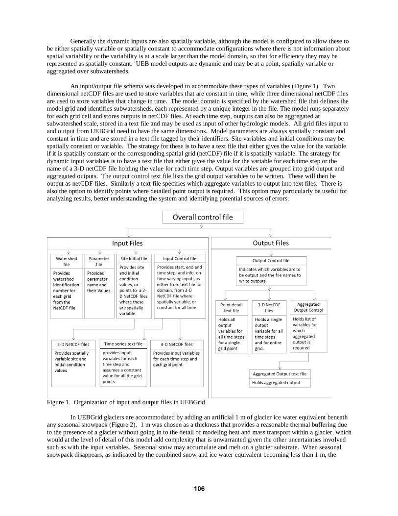
Generally the dynamic inputs are also spatially variable, although the model is configured to allow these to be either spatially variable or spatially constant to accommodate configurations where there is not information about spatial variability or the variability is at a scale larger than the model domain, so that for efficiency they may be represented as spatially constant. UEB model outputs are dynamic and may be at a point, spatially variable or aggregated over subwatersheds. An input/output file schema was developed to accommodate these types of variables (Figure 1). Two dimensional netCDF files are used to store variables that are constant in time, while three dimensional netCDF files are used to store variables that change in time. The model domain is specified by the watershed file that defines the model grid and identifies subwatersheds, each represented by a unique integer in the file. The model runs separately for each grid cell and stores outputs in netCDF files. At each time step, outputs can also be aggregated at subwatershed scale, stored in a text file and may be used as input of other hydrologic models. All grid files input to and output from UEBGrid need to have the same dimensions. Model parameters are always spatially constant and constant in time and are stored in a text file tagged by their identifiers. Site variables and initial conditions may be spatially constant or variable. The strategy for these is to have a text file that either gives the value for the variable if it is spatially constant or the corresponding spatial grid (netCDF) file if it is spatially variable. The strategy for dynamic input variables is to have a text file that either gives the value for the variable for each time step or the name of a 3-D netCDF file holding the value for each time step. Output variables are grouped into grid output and aggregated outputs. The output control text file lists the grid output variables to be written. These will then be output as netCDF files. Similarly a text file specifies which aggregate variables to output into text files. There is also the option to identify points where detailed point output is required. This option may particularly be useful for analyzing results, better understanding the system and identifying potential sources of errors.
Figure 1. Organization of input and output files in UEBGrid In UEBGrid glaciers are accommodated by adding an artificial 1 m of glacier ice water equivalent beneath any seasonal snowpack (Figure 2). 1 m was chosen as a thickness that provides a reasonable thermal buffering due to the presence of a glacier without going in to the detail of modeling heat and mass transport within a glacier, which would at the level of detail of this model add complexity that is unwarranted given the other uncertainties involved such as with the input variables. Seasonal snow may accumulate and melt on a glacier substrate. When seasonal snowpack disappears, as indicated by the combined snow and ice water equivalent becoming less than 1 m, the
106
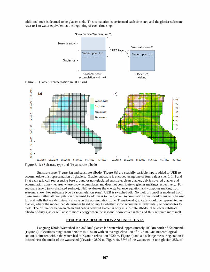
additional melt is deemed to be glacier melt. This calculation is performed each time step and the glacier substrate reset to 1 m water equivalent at the beginning of each time step.
Figure 2. Glacier representation in UEBGrid
Figure 3. (a) Substrate type and (b) substrate albedo Substrate type (Figure 3a) and substrate albedo (Figure 3b) are spatially variable inputs added to UEB to accommodate this representation of glaciers. Glacier substrate is encoded using one of four values (i.e. 0, 1, 2 and 3) at each grid cell representing bare ground or non-glaciated substrate, clean glacier, debris covered glacier and accumulation zone (i.e. area where snow accumulates and does not contribute to glacier melting) respectively. For substrate type 0 (non-glaciated surface), UEB evaluates the energy balance equation and computes melting from seasonal snow. For substrate type 3 (accumulation zone), UEB is switched off. No melt or runoff is modeled from these areas, rather all precipitation presumed to add mass to the glacier. Accumulation zone should thus only be used for grid cells that are definitively always in the accumulation zone. Transitional grid cells should be represented as glacier, where the model then determines based on inputs whether snow accumulates indefinitely or contributes to melt. The difference between clean and debris covered glacier is only in substrate albedo. The lower substrate albedo of dirty glacier will absorb more energy when the seasonal snow cover is thin and thus generate more melt.
STUDY AREA DESCRIPTION AND INPUT DATA Langtang Khola Watershed is a 363 km2 glacier fed watershed, approximately 100 km north of Kathmandu (Figure 4). Elevations range from 3700 m to 7184 m with an average elevation of 5176 m. One meteorological station is situated within the watershed at Kyanjin (elevation 3920 m, Figure 4) and a discharge measuring station is located near the outlet of the watershed (elevation 3800 m, Figure 4). 57% of the watershed in non-glacier, 35% of
107

area is occupied by clean glacier and 8% of area is covered by dirty or debris-cover glacier. Glacier outline maps for Langang Khola watershed were derived from Advanced Spaceborne Thermal Emission and Reflection Radiometer (ASTER) images from October 2003, ortho-rectified products (ASTDMO14). The scenes had high contrast over glaciers, minimal cloud cover, and were acquired at the end of the ablation season (for minimal seasonal snow), and hence are suitable for glacier mapping. Substrate albedo was derived from the atmospherically corrected surface reflectance product (AST_07XT). Elevation, slope and aspect was derived from Shuttle Radar Topography Mission (SRTM) digital elevation model data. The watershed is divided into grids with resolution of 0.0008333̊ .
Figure 4. Langtang Khola Watershed. Subwatershed shown in hatched area is used as an example to illustrate substrate type and substrate albedo representation in Figure 2. A three-hour time step was used. Six-hourly temperature and daily precipitation from the metrological station at Kyanjin (Figure 4) is used in this simulation. Three-hourly temperature data was derived using linear interpolation of six-hourly data and daily precipitation was uniformly divided into eight three hourly time steps to obtained three-hourly precipitation. A vertical lapse rate was applied to both precipitation and temperature. Our examination of the literature did not identify a definitive way to select lapse rates to use in the HKH region. Immerzeel et al. (2012) used temperature lapse rate of 6.3 ˚C/km in their study of hydrological responses of Langtang watershed in a changing climate. Kayastha et al. (1999) used 6 ˚C/km in a water balance model in this region. Fujita and Sakai (1996) conducted a study to observe the lapse rate in Langtang Valley over the time period of May to Oct, 1996. Data was collected at three different locations in their study, (1) Base house as reference site (3878 m a. s. l.), (2) Lirung Glacier (5350 m a. s. l.), and (3) Lirung Glacier (4153 m a. s. l.). Estimates for the two glaciers differed due to their topography. Although daily mean lapse rate for those glaciers was close (i.e. 5.1 ˚C/km for Lirung and 5.4 ̊ C/km for Yala), the lapse rate at Ligung glacier had a much more distinct diurnal and seasonal pattern than Yala. Yala is located on an open slope and had relatively less fluctuation of lapse rate. Lirung glacier, located at the bottom of a deep valley, consists of heterogeneous debris topology. Relatively high fluctuation in both seasonal and diurnal lapse rate was observed at Lirung. Fujita and Sakai concluded that spatial variation for this region cannot be represented by a simple constant lapse rate. Nevertheless we decided to use a constant lapse rate of 6.0 ˚C/km for this study because we did not have sufficient information to do anything more elaborate. Precipitation also generally varies with topography. Ageta et al. (1980) and Kayastha et al. (1999) found negligible variation in precipitation distribution due to change in elevation in this region. However in a more recent
108
study Immerzeel et al. (2012) suggested a vertical precipitation lapse rate of 0.04 percent/m increase. We used this value. Relative humidity and wind speed used in this study were obtained from NASA Modern-Era Retrospective Analysis for Research and Applications (MERRA) ½° latitude × ⅔° longitude data (Rienecker et al., 2011). This was downscaled using methods based on MicroMet (Liston and Elder, 2006). Incoming shortwave radiation was calculated within UEB using diurnal temperature range, time of day, date, slope and aspect. Incoming longwave radiation was also computed in the model using air temperature, air vapor pressure and cloudiness fraction.
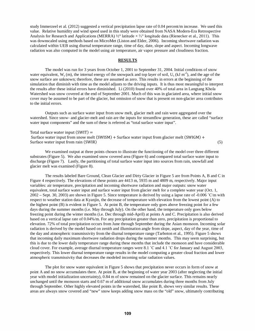
RESULTS The model was run for 3 years from October 1, 2001 to September 31, 2004. Initial conditions of snow water equivalent, Ws (m), the internal energy of the snowpack and top layer of soil, Us (kJ m-2), and the age of the snow surface are unknown; therefore, these are assumed as zero. This results in errors at the beginning of the simulation that diminish with time as the model adjusts to the driving inputs. It is thus most meaningful to interpret the results after these initial errors have diminished. Li (2010) found over 40% of total area in Langtang Khola Watershed was snow covered at the end of September 2001. Much of this was in glaciated area, where initial snow cover may be assumed to be part of the glacier, but omission of snow that is present on non-glacier area contributes to the initial errors. Outputs such as surface water input from snow melt, glacier melt and rain were aggregated over the watershed. Since snow- and glacier-melt and rain are the inputs for streamflow generation, these are called “surface water input components” and the sum of these is referred as “total surface water input”. Total surface water input (SWIT) = Surface water input from snow melt (SWISM) + Surface water input from glacier melt (SWIGM) +Surface water input from rain (SWIR) (5) We examined output at three points chosen to illustrate the functioning of the model over three different substrates (Figure 5). We also examined snow covered area (Figure 6) and compared total surface water input to discharge (Figure 7). Lastly, the partitioning of total surface water input into sources from rain, snowfall and glacier melt was examined (Figure 8). The results labeled Bare Ground, Clean Glacier and Dirty Glacier in Figure 5 are from Points A, B and C in Figure 4 respectively. The elevations of these points are 4413 m, 5935 m and 4809 m, respectively. Major input variables: air temperature, precipitation and incoming shortwave radiation and major outputs: snow water equivalent, total surface water input and surface water input from glacier melt for a complete water year (Oct. 1, 2002 – Sept. 30, 2003) are shown in Figure 5. Since temperature is derived by using a lapse rate of -0.006 ˚C/m with respect to weather station data at Kyanjin, the decrease of temperature with elevation from the lowest point (A) to the highest point (B) is evident in Figure 5. At point B, the temperature only goes above freezing point for a few days during the summer months (i.e. May through July). On the other hand, the temperature only goes below freezing point during the winter months (i.e. Dec through mid-April) at points A and C. Precipitation is also derived based on a vertical lapse rate of 0.04%/m. For any precipitation greater than zero, precipitation is proportional to elevation. 72% of total precipitation occurs from June through September during the Asian monsoon. Incoming solar radiation is derived by the model based on zenith and illumination angle from slope, aspect, day of the year, time of the day and atmospheric transmissivity from the diurnal temperature range (Tarboton et al., 1995). Figure 5 shows that incoming daily maximum shortwave radiation drops during the summer months. This may seem surprising, but this is due to the lower daily temperature range during these months that include the monsoon and have considerable cloud cover. For example, average diurnal temperature ranges were 8.1 ˚C and 4.1 ˚C for January and August 2003, respectively. This lower diurnal temperature range results in the model computing a greater cloud fraction and lower atmospheric transmissivity that decreases the modeled incoming solar radiation values. The plot for snow water equivalent in Figure 5 shows that precipitation never occurs in form of snow at point A and no snow accumulates there. At point B, at the beginning of water year 2003 (after neglecting the initial year with model initialization uncertainty), 0.84 m of snow remained on the glacier surface. This remains nearly unchanged until the monsoon starts and 0.67 m of additional snow accumulates during three months from July through September. Other highly elevated points in the watershed, like point B, shows very similar results. These areas are always snow covered and “new” snow keeps adding snow mass on the “old” snow, ultimately contributing
109
input to the glaciers. No melt was modeled to occur at point B (Figure 5, Total surface water input). At point A, precipitation throughout the year generated surface water input, with a concentration during the monsoon season (Figure 5, Total surface water input). At Point C, on the other hand, total surface water input was generated from all three possible sources, namely rain, snow and glacier melt. Snow accumulates from February to mid-April and then melts away by mid-May. Precipitation occurs in form of rain mostly during the monsoon and a large amount of glacier also melts during the same season. Thus, we can conclude that during the monsoon large amounts of surface water input are from the combination of rain, snow- and glacier-melting at lower elevations, while at high elevations the monsoon snow accumulates and adds to glacier ice. Although the temperature is below freezing over the majority of the watershed during winter, due to sparse precipitation, snow accumulation is relatively small.
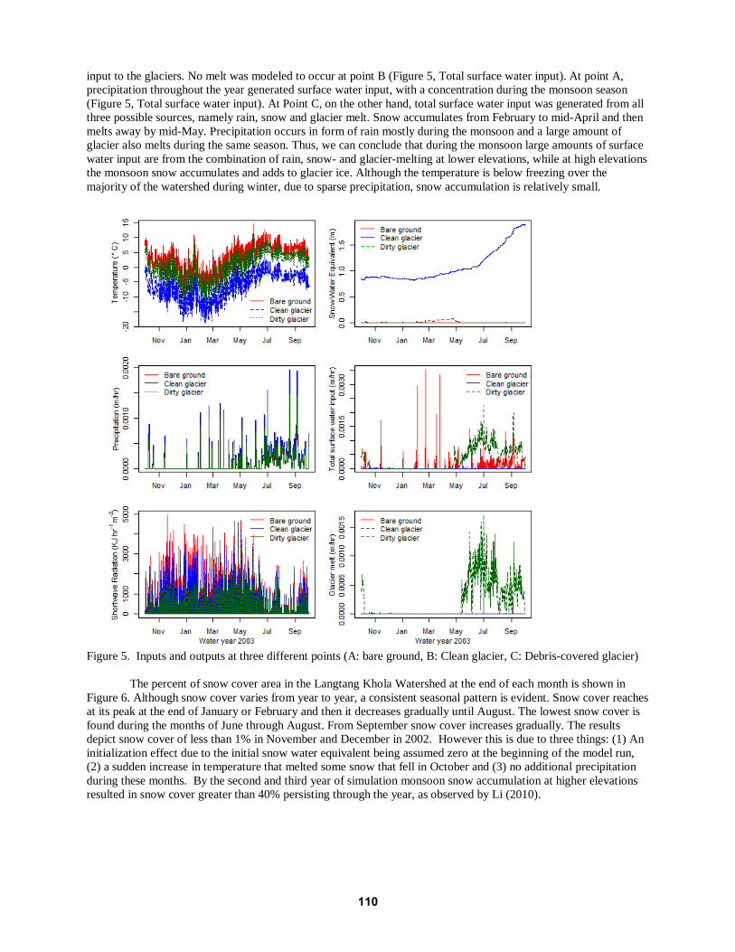
Figure 5. Inputs and outputs at three different points (A: bare ground, B: Clean glacier, C: Debris-covered glacier) The percent of snow cover area in the Langtang Khola Watershed at the end of each month is shown in Figure 6. Although snow cover varies from year to year, a consistent seasonal pattern is evident. Snow cover reaches at its peak at the end of January or February and then it decreases gradually until August. The lowest snow cover is found during the months of June through August. From September snow cover increases gradually. The results depict snow cover of less than 1% in November and December in 2002. However this is due to three things: (1) An initialization effect due to the initial snow water equivalent being assumed zero at the beginning of the model run, (2) a sudden increase in temperature that melted some snow that fell in October and (3) no additional precipitation during these months. By the second and third year of simulation monsoon snow accumulation at higher elevations resulted in snow cover greater than 40% persisting through the year, as observed by Li (2010).
110
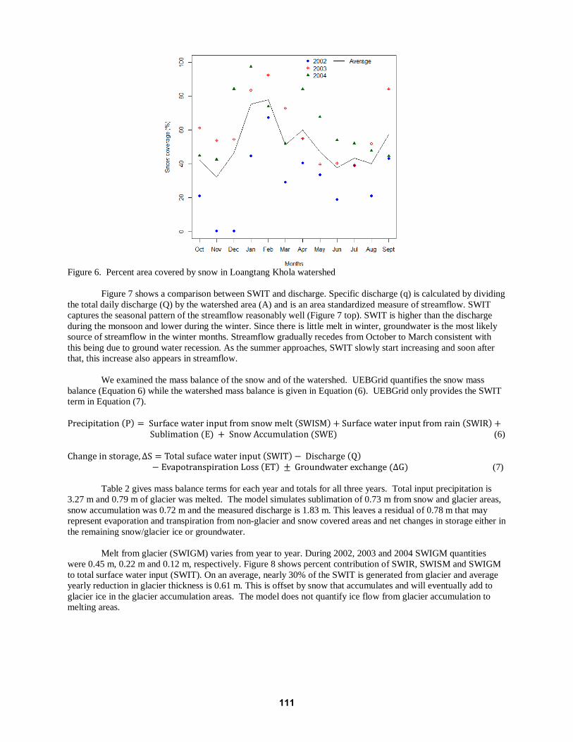
Figure 6. Percent area covered by snow in Loangtang Khola watershed Figure 7 shows a comparison between SWIT and discharge. Specific discharge (q) is calculated by dividing the total daily discharge (Q) by the watershed area (A) and is an area standardized measure of streamflow. SWIT captures the seasonal pattern of the streamflow reasonably well (Figure 7 top). SWIT is higher than the discharge during the monsoon and lower during the winter. Since there is little melt in winter, groundwater is the most likely source of streamflow in the winter months. Streamflow gradually recedes from October to March consistent with this being due to ground water recession. As the summer approaches, SWIT slowly start increasing and soon after that, this increase also appears in streamflow. We examined the mass balance of the snow and of the watershed. UEBGrid quantifies the snow mass balance (Equation 6) while the watershed mass balance is given in Equation (6). UEBGrid only provides the SWIT term in Equation (7). Precipitation (P) = Surface water input from snow melt (SWISM) + Surface water input from rain (SWIR) + Sublimation (E) + Snow Accumulation (SWE) (6) Change in storage,ΔS = Total suface water input (SWIT)− Discharge (Q) − Evapotranspiration Loss (ET) ± Groundwater exchange (ΔG) (7) Table 2 gives mass balance terms for each year and totals for all three years. Total input precipitation is 3.27 m and 0.79 m of glacier was melted. The model simulates sublimation of 0.73 m from snow and glacier areas, snow accumulation was 0.72 m and the measured discharge is 1.83 m. This leaves a residual of 0.78 m that may represent evaporation and transpiration from non-glacier and snow covered areas and net changes in storage either in the remaining snow/glacier ice or groundwater. Melt from glacier (SWIGM) varies from year to year. During 2002, 2003 and 2004 SWIGM quantities were 0.45 m, 0.22 m and 0.12 m, respectively. Figure 8 shows percent contribution of SWIR, SWISM and SWIGM to total surface water input (SWIT). On an average, nearly 30% of the SWIT is generated from glacier and average yearly reduction in glacier thickness is 0.61 m. This is offset by snow that accumulates and will eventually add to glacier ice in the glacier accumulation areas. The model does not quantify ice flow from glacier accumulation to melting areas.
111

Figure 7. Comparison between melt estimated by UEBGrid and specific discharged measured at Kyangjin hydrologic station. Table 2: Mass balance quantities Year Specific
discharge, q (m)
Precipitation, P (m)
Surface water input from snow melt, SWISM (m)
Surface water input from rain, SWIR (m)
Snow water equivalent, SWE (m)
Sublimation, E (m)
2002 0.63 1.13 0.30 0.48 0.17 0.21 2003 0.59 1.10 0.35 0.24 0.26 0.26 2004 0.61 1.04 0.29 0.19 0.31 0.26 Total 1.83 3.27 0.94 0.91 0.72 0.73
DISCUSSION AND CONCLUSION The Utah Energy Balance Snowmelt model has been extended to in a simple way calculate the melting of glaciers as well as accumulation and melting of snow. It has been refactored so that it can be applied over a grid using netCDF files to manage input-output workflow and data storage. This refactoring provides the capability to drive the model using NASA remote sensing and earth science data products. In the current study, wind speed and relative humidity data were obtained from downscaled Modern-Era Retrospective Analysis for Research and Applications (MERRA), while air temperature and precipitation were derived from observation data at Kyanjin weather station using vertical lapse rate. Incoming short and longwave radiation were calculated by UEBGrid. In future work we plan to evaluate the use of MERRA data as a source for all these variables so as to extend the application of the model to locations where this ground based data is not available. UEBGrid introduces a simple way to represent glaciers using glacier outline and albedo maps. The model estimates an average of 0.61 m/year of glacier melting over the glacier area within the Langtang Khola Watershed for the 3 year study period (water years 2002-2004). Melt from debris-covered glacier is a complicated process. Melt from the debris-covered glaciers may be over-estimated due to debris inhibiting the surface energy exchanges where there is a thick debris-layer present on glacier (Brock et al., 2010). On the other hand, presence of a thin debris layer may increase the melt, as debris-
112

cover has low albedo (Kayastha et al., 2000). Due to lack of observation data on debris thickness we were unable to include debris thickness into the model. Lack of ability to quantify these effects introduces additional uncertainty to the melt from debris-covered glaciers. Quantification of debris thickness is considered to be an important step towards better prediction of melt from debris-covered glaciers.
Figure 8. Contribution from rain, snow and glacier in Total Surface Water Input (SWIT)
ACKNOWLEDGEMENTS
This research was supported by NASA award NNX11AK036. The authors are especially thankful to Adina Racoviteanu from Laboratoire de Glaciologie et Géophysique de l'Environnement for providing glacier mapping and substrate albedo data. Authors would also like to thank Dr. Mandira Shrestha from ICIMOD for proving streamflow data.
REFERENCES Ageta, Y., Ohata, T., Tanaka, Y., Ikegami, K. and Higuchi, K. 1980. Mass balances of Glacier AX010, in Shorong Himal during the summer monsoon season, East Nepal. In: Higuchi, K., Hakajima, C. and Kusunoki, K., eds. Glaicers and Climates of Nepal Himalayas. Report of the Glaciological Expedition to Nepal: Part 4. Seppyo, Special Issue, no. 41: 34-41. Barnett, T. P., J. C. Adam and D. P. Lettenmaier, (2005), Potential impacts of a warming climate on water availability in snow-dominated regions, Nature, 438(7066): 303-309. Brock, B. W., C. Mihalcea, M. P. Kirkbride, G. Diolaiuti, M. E. Cutler and C. Smiraglia, (2010), Meteorology and surface energy fluxes in the 2005–2007 ablation seasons at the Miage debris‐covered glacier, Mont Blanc Massif, Italian Alps, Journal of Geophysical Research: Atmospheres (1984–2012), 115(D9). Brown, M. E., H. Ouyang, S. Habib, B. Shrestha, M. Shrestha, P. Panday, M. Tzortziou, F. Policelli, G. Artan and A. Giriraj, (2010), HIMALA: Climate Impacts on Glaciers, Snow, and Hydrology in the Himalayan Region, Mountain Research and Development, 30(4): 401-404. Hall, D. K., G. A. Riggs, V. V. Salomonson, N. E. DiGirolamo and K. J. Bayr, (2002), MODIS snow-cover products, Remote sensing of Environment, 83(1): 181-194. Immerzeel, W. W., L. Van Beek, M. Konz, A. Shrestha and M. Bierkens, (2012), Hydrological response to climate change in a glacierized catchment in the Himalayas, Climatic Change, 110(3-4): 721-736.
113
Kayastha, R. B., Y. Takeuchi, M. Nakawo and Y. Ageta, (2000), Practical prediction of ice melting beneath various thickness of debris cover on Khumbu Glacier, Nepal, using a positive degree-day factor, IAHS PUBLICATION: 71-82. Kehrwald, N. M., L. G. Thompson, Y. Tandong, E. Mosley‐Thompson, U. Schotterer, V. Alfimov, J. Beer, J. Eikenberg and M. E. Davis. 2008. Mass loss on Himalayan glacier endangers water resources, Geophysical Research Letters, 35(22). Lamadrid, A. J. and K. L. MacClune. 2010. Climate and hydrological modeling in the Hindu-Kush Himalaya region., http://www.i-s-e-t.org/images/pdfs/climate%20and%20hydrological%20modeling%20in%20the%20hindu-kush.pdf. Li, X. 2010. Mountainous snow cover monitoring and snowmelt runoff discharge modeling in the Langtang Khola catchment. Liston, G. E. and K. Elder, (2006), A meteorological distribution system for high-resolution terrestrial modeling (MicroMet), Journal of Hydrometeorology, 7(2): 217-234. Luce, C. H. and D. G. Tarboton, (2004), The Application of Depletion Curves for Parameterization of Subgrid Variability of Snow, Hydrological Processes, 18: 1409-1422, DOI: 10.1002/hyp.1420. Luce, C. H. and D. G. Tarboton, (2010), Evaluation of alternative formulae for calculation of surface temperature in snowmelt models using frequency analysis of temperature observations, Hydrol. Earth Syst. Sci., 14(3): 535-543, http://www.hydrol-earth-syst-sci.net/14/535/2010/. Mahat, V., (2011), Effect of Vegetation on the Accumulation and Melting of Snow at the TW Daniels Experimental Forest, Ph.D. Thesis, Civil and Env.t'l Eng., Utah State Univ., http://digitalcommons.usu.edu/etd/1078, 181 pp. Mahat, V. and D. G. Tarboton. 2012. Canopy radiation transmission for an energy balance snowmelt model, Water Resour. Res., 48: W01534, http://dx.doi.org/10.1029/2011WR010438. Mahat, V., D.G. Tarboton, and N.P. Molotch, (2013), Testing above and below canopy representations of turbulent fluxes in an energy balance snowmelt model, Water Resources Res., 49(2): 1107-1122, http://dx.doi.org/10.1002/wrcr.20073. Racoviteanu, A. E., M. W. Williams and R. G. Barry. 2008. Optical remote sensing of glacier characteristics: a review with focus on the Himalaya, Sensors, 8(5): 3355-3383. Rahaman, M.M. 2002. Bangladesh–from a country of flood to a country of water scarcity–sustainable perspectives for solution, Ratio: 2. Rew, R. and G. Davis, (1990), NetCDF: an interface for scientific data access, Computer Graphics and App., IEEE, 10(4): 76-82. Rew, R., G. Davis, S. Emmerson, H. Davies and E. Hartnett. 1993. NetCDF User's Guide, Unidata Program Center, Boulder, CO. Rienecker, M.M., M.J. Suarez, R. Gelaro, R. Todling, J. Bacmeister, E. Liu, M.G. Bosilovich, S.D. Schubert, L. Takacs and G.K. Kim. 2011. MERRA: NASA's modern-era retrospective analysis for research and applications, J. of Climate, 24(14): 3624-3648. Tarboton, D. G., T. G. Chowdhury and T. H. Jackson. 1995. A Spatially Distributed Energy Balance Snowmelt Model, in Biogeochemistry of Seasonally Snow-Covered Catchments (Proc. of a Boulder Symposium, July 1995), Ed. by K. A. Tonnessen, M. W. Williams and M. Tranter, IAHS Publ. no. 228, Wallingford, p.141-155, http://iahs.info/redbooks/a228/iahs_228_0141.pdf. Tarboton, D. G. and C. H. Luce. 1996. Utah Energy Balance Snow Accumulation and Melt Model (UEB), Computer model technical description and users guide, Utah Water Research Laboratory and USDA Forest Service Intermountain Research Station (http://www.engineering.usu.edu/dtarb/), Logan, Utah, 64 p. Tarboton, D. G., K. Williams and C. Luce, (1996), Development and Testing of a Parsimonious Energy Balance Snowmelt Model, Eos Trans. AGU, 77(46): AGU Fall Meeting Suppl., F219, Invited present. at American Geophys. Union Fall Meeting. Thapa, K., (1993), Estimation of snowmelt runoff in Himalayan catchments incorporating remote sensing data, IAHS Publications-Publications of the International Association of Hydrological Sciences, 218: 69-74. Vörösmarty, C. J., P. Green, J. Salisbury and R. B. Lammers. 2000. Global Water Resources: Vulnerability from Climate Change and Population Growth, Science, 289(5477): 284-288, http://dx.doi.org/10.1126/science.289.5477.284. You, J. 2004. Snow Hydrology: The Parameterization of Subgrid Processes within a Physically Based Snow Energy and Mass Balance Model, PhD Thesis, Civil and Environmental Engineering, Utah State University.
114