USING THE ECOSYSTEM SERVICE VALUE OF HABITAT AREAS FOR WILDLIFE

CONSERVATION:

IMPLICATIONS OF CARBON-RICH PEATSWAMP FORESTS FOR THE

BORNEAN ORANG-UTAN, Pongo pygmaeus

by

Megan Cattau

Dr. Dean Urban, Advisor

May 2010

Masters project submitted in partial fulfillment of the

requirements for the Master of Environmental Management degree in

the Nicholas School of the Environment of

Duke University

2010

i

Abstract

Forest fragmentation and degradation of lowland tropical peatswamp forests in Borneo pose a serious threat to the endangered Bornean orang-utan, whose decreasing population trends are attributed primarily to habitat loss. The orang-utan is projected to be extinct by 2020 unless existing populations can be connected and new conservation areas established, which is not currently economically viable. However, peatswamp forests, on which orang-utans can be found at their greatest densities, have a large capacity for carbon sequestration and storage and, thus, a high potential value on the carbon market. Unfortunately, as these wetlands are being deforested, drained, and burned for development, the peat soil is decomposing, emitting CO2 into the atmosphere, and impacting global climate change. This project is a spatially explicit analysis of an area of fragmented peatswamp forest in Central Kalimantan, Indonesia that explores how the conservation targets of ape preservation and carbon sequestration and storage can be mutually satisfied through land management strategies. First, I prioritized intact peatswamp forest patches for conservation based on orang-utan presence and patch geometry metrics. To do this, I surveyed line transects in the study area, Block C of the Former Mega Rice Project, for orang-utan sleeping nests and produced a regional density estimate of 2.517 individuals / km2. I identified patches greater than 350 ha from Landsat 7 TM data and then calculated the number of individuals and patch geometry metrics for each patch. I found the total population on Block C to be 2,161 individuals, only 1,146 of which are located in forest fragments with a population size large enough to be considered viable. I generated a model of habitat suitability for the orang-utan using maximum entropy methods. Then, I proposed corridors through degraded areas between the six priority patches of intact forest using least-cost path methods. The corridors included areas of high habitat suitability and also areas of high carbon value, and would increase the viable population size of orang-utans to 1,788 individuals. This project demonstrates how the incentive of carbon financing can make possible wildlife protection strategies, and how we might begin to use spatial planning to maximize biodiversity and ecosystem service benefits on the landscape.

Keywords: Borneo, carbon market, conservation planning, habitat corridor, orang-utan, peat

ii

Acknowledgements

This project could not have taken place without the generous support of several people. I would like to first thank my advisor, Dr. Dean Urban, who offered his expertise, patience, and advice through the entire process, and Dr. Jennifer Swenson, who is an expert in all things geospatial.

I would like to thank Orang-utan Tropical Peatland Project for offering support

during the field study portion of this project. In particular, I would like to thank Dr. Susan Cheyne, who provided continued support and advice in the field, and Simon Husson, who offered his expertise concerning orang-utan density analysis. I would like to thank my field assistants who made data collection possible. I would especially like to thank my field assistants Hedri, Ari, and Juliansya, who were with me through the entire data collection process, not only offering research support, but also their humor, kindness, and wilderness survival skills.

I would also like to acknowledge the financial support of the Kuzmier-Lee-

Nikitine Endowment Fund, the SIDG-Lazar Foundation, the Nicholas School International Internship Fund, and the Orang-utan Foundation, without which this research could not have been possible.

iii

Table of Contents ABSTRACT ................................................................................................................... I ACKNOWLEDGEMENTS ...............................................................................................II LIST OF FIGURES ........................................................................................................ IV ABBREVIATIONS........................................................................................................ IV INTRODUCTION .......................................................................................................... 1 PEATSWAMP FOREST DEGRADATION AND THE ORANG-UTAN ...................................................... 1 PEATLAND DEGRADATION AND CLIMATE ................................................................................ 3 CLEAN DEVELOPMENT MECHANISM (CDM) AND REDUCING EMISSIONS FROM DEFORESTATION AND

DEGRADATION (REDD) AS CONSERVATION MECHANISMS .............................................. 4 STUDY AREA: BLOCK C OF THE FORMER MEGA RICE PROJECT ...................................................... 6 OBJECTIVES .................................................................................................................... 9 METHODS ................................................................................................................... 9 2.1 PATCH PRIORITIZATION .............................................................................................. 10 LAND USE / LAND COVER CLASSIFICATION, ORANG-UTAN HABITAT PATCH IDENTIFICATION, AND PATCH

GEOMETRY ............................................................................................................... 10 ORANG-UTAN PRESENCE ......................................................................................................... 14 2.2 CORRIDOR IDENTIFICATION ......................................................................................... 20 SPECIES DISTRIBUTION MODEL ................................................................................................. 21 CORRIDORS ........................................................................................................................... 24 RESULTS.................................................................................................................... 27 3.1 PATCH PRIORITIZATION .............................................................................................. 27 LAND USE / LAND COVER CLASSIFICATION, ORANG-UTAN HABITAT PATCH IDENTIFICATION, AND PATCH

GEOMETRY ............................................................................................................... 27 ORANG-UTAN PRESENCE ......................................................................................................... 33 3.2 CORRIDOR IDENTIFICATION ......................................................................................... 37 SPECIES DISTRIBUTION MODEL ................................................................................................. 37 CORRIDORS ........................................................................................................................... 41 DISCUSSION .............................................................................................................. 43 LITERATURE CITED .................................................................................................... 48 APPENDIX A: RADIOMETRIC AND ATMOSPHERIC CORRECTION OF SATELLITE DATA ... 52 APPENDIX B: VARIABLES USED IN MAXENT DISTRIBUTION MODEL ............................ 54

iv

List of Figures

Figure 1. Study Area: Block C of the former Mega Rice Project in Central Kalimantan, Indonesia (Borneo). ................................................................................................ 8

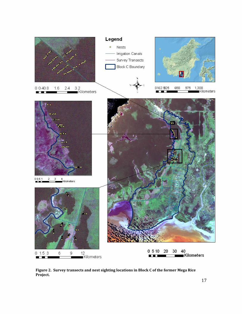
Figure 2. Survey transects and nest sighting locations in Block C of the former Mega Rice Project. .................................................................................................................. 17

Figure 3. Cost Surfaces for corridor paths consisting of the maxent species distribution model, aboveground and belowground carbon stock, and a combined surface. 26

Figure 4. Land cover classes and orang-utan habitat patches in Block C of the Mega-Rice Project ................................................................................................................... 28

Figure 5. Patch Geometry Metrics computed for the orang-utan habitat patches: area, patch thickness, shape index, and core-area ratio. .............................................. 31

Figure 6. Patch prioritization of orang-utan habitat patches based solely on patch geometry metrics. ................................................................................................. 32

Figure 7. Orang-utan density and number of orang-utan individuals by patch. ............. 35 Figure 8. Priority patches based on patch geometry metrics and orang-utan presence. 36 Figure 9. Jackknife test of variable importance produced by Maxent . .......................... 39 Figure 10. Maxent Species Distribution Model. .............................................................. 40 Figure 11. Corridor Paths between habitat patches without and with carbon value

considered. ............................................................................................................ 42 Figure 12. Six of the predictor variables entered into the Maxent model. ..................... 54 Figure 13. Five of the predictor variables entered into the Maxent model. ................... 55

Abbreviations

CDM Clean Development Mechanism CIMTROP Centre for International Cooperation in the Sustainable

Management of Tropical Peatland COP Conference of the Parties LULC Land Use / Land Cover OuTROP Orang-utan Tropical Peatland Project PSF Peatswamp Forest REDD Reduced Emissions from avoided Degradation and Deforestation UNFCC United Nations Framework Convention on Climate Change

1

Introduction

The lowland peatswamp forests in Kalimantan, Indonesia, provide invaluable

ecosystem services to the nearby human populations, as they buffer saltwater intrusion

(Boehm and Siegert, 1999), prevent flooding problems downstream, and resist large-

scale fires (Yule, 2010). Additionally, of great importance to the international

community, peatlands have a large capacity for belowground carbon sequestration and

storage and, thus, a high potential to slow global climate change. They are also rich in

endemic flora and fauna (Yule, 2010). However, peatland areas all over Southeast Asia

are being degraded and fragmented due, in large part, to the development of oil palm

and timber plantations, agriculture, and logging (Hoojier et al. 2006). The lowland areas

are being targeted for agricultural development primarily because they are more

accessible and thus easier to cultivate than mountainous areas. In recent years, large,

monoculture oil palm (Elaeis guineensis) plantations in particular have expanded rapidly

in response to international demand for the various products that are manufactured

from the palm’s oil. In fact, between 1984 and 2003, the area planted with oil palm on

Borneo increased from 2,000 km² to 27,000 km², about 10,000 km² of which is located

in Kalimantan (Ancrenaz et al., 2008).

Peatswamp Forest Degradation and The Orang-utan

As these lowland peatswamp forest fragments become sparser and more

fragmented, species that depend on these wetlands for habitat or breeding are

2

dwindling. Of particular note are the Bornean and Sumatran orang-utans. The orang-

utan, the only great ape in Asia, can be found solely on the Indonesian island of Sumatra

and on the Malaysian and Indonesian areas of the island of Borneo, with separate

species on each island. The Bornean orang-utan (Pongo pygmaeus) is currently

classified an endangered by The International Union for Conservation of Nature (IUCN),

and the Sumatran orang-utan (Pongo abelii) is classified as critically endangered. Both

species have decreasing population trends, attributed primarily to forest loss due to

conversion of forest to agriculture and to forest fires (Ancrenaz et al., 2008). The

majority of the animals are living outside of protected areas in forests that are being

converted to agriculture and that are vulnerable to timber harvesting. A study by

Goossens et al. (2006) in which the largest-yet genetic sample of wild orang-utan

populations was used, demonstrates a recent demographic collapse of orang-utans in

North Eastern Borneo. This study quantifies the effects of anthropogenic deforestation

and habitat fragmentation on the apes and supports the need for major conservation

efforts for the genetic viability of the species. In fact, it is predicted that the orang-utan

will be completely extinct by the second decade of this century unless drastic

conservation actions are taken, including establishing new conservation areas and

expanding and connecting existing ones (Rijksen and Meijaard, 1999).

The orang-utan, one of four great apes in the same taxonomic group as our

species (Homo sapiens) has been historically viewed as a human relative, and is often

protected out of respect for its intrinsic value (Rijksen and Meijaard 1999). Thus, their

3

appeal to human empathy can make them an umbrella species for conservation efforts

in their habitat area. Additionally, the very health of the rainforests, which provide

ecosystem services to human beings, are dependent on the orang-utan, as these apes

play an essential role in seed dispersal, particularly for large seeds that are not

dispersed by smaller animals (Ancrenaz et al. 2006). Orang-utans favor the lowlands,

namely alluvial flood plains, peatswamp forests, and valleys (Rijksen and Meijaard

1999), with the greatest density occurring in peatswamp forests. The animals are found

in greater densities in the lowlands because these areas produce more regular and

larger fruit crops than dry dipterocarp forests (Ancrenaz et al. 2005). Thus, there is

conservation reciprocity between the peatswamp forest and the orang-utan, with the

peatswamp forests providing necessary habitat for the orang-utan, and the orang-utan

providing seed-dispersing services for the peatswamp forest.

Peatland Degradation and Climate

For agricultural use, the peatlands must first be deforested, drained, and burned.

Draining peat soils precludes them from being a further carbon sink, as this impedes

their ability to accumulate additional organic matter, but it also releases the carbon

already stored in them. As the soils are drained, the resulting aeration and

decomposition of the peat leads to oxidation and, thus, CO2 emission (Hooijer et al.

2006). In a project titled the Peat-CO2 project, emissions caused by the decomposition

of drained peatlands were estimated based on data of peat depth and extent, present

and projected land use and water management practice, decomposition rates, and fire

4

emissions. Emissions were determined to be 632 Megatonnes/year (Mt/y) as of 2006.

An additional 1400 Mt/y in CO2 emissions was attributed to peatland fires. This some

2000 Mt/y (over 90% of which comes from Indonesia) accounts for nearly 8% of global

emissions from fossil fuel burning. Additionally, it is projected that emissions will

increase if current land management practices remain the same (Hooijer et al. 2006).

Peat fires pose an additional threat to the available carbon stock in peatlands.

As the soil is aerated from forest clearing or irrigation canals, the peat is much more

susceptible to ignition. Peat fires typically burn aboveground and belowground not only

directly affecting individual tree species, but also destroying the seedbank and the peat,

which may take thousands of years to replace (Yeager, 1999). Fires are a major threat

to the continued existence of the endangered orang-utan (Yeager and Fredriksson,

1999).

Clean Development Mechanism (CDM) and Reducing Emissions from

Deforestation and Degradation (REDD) as Conservation Mechanisms

In light of the global implications of climate change, there is a clear need for an

economically viable way for Indonesia to reduce its greenhouse gas emissions through

land and water management practices, specifically through peatland forest preservation

and restoration. The carbon market may provide opportunities for this to be possible.

The Kyoto Protocol, adopted by Conference of the Parties (COP) 3 in 1997, is the

main mechanism guiding greenhouse gas emissions reductions worldwide. Under the

Kyoto Protocol, Annex I countries, or industrialized countries, that have ratified the

5

protocol have committed themselves to reducing their emissions by a target percentage

from the 1990 baseline by 2012. Several flexible mechanisms were approved by the

United Nations Framework Convention on Climate Change (UNFCCC) that allow Annex I

countries to meet their emissions reductions goals, including International Emissions

Trading (EIT), the Clean Development Mechanism (CDM), and Joint Implementation (JI).

The CDM and JI are project-based emissions reduction mechanisms, in which Annex I

countries can fund projects in non-Annex I or Annex I countries, respectively, that

produce emissions reductions. Credits are given for the emissions that are avoided

compared to a baseline of emissions in the absence of the project. Currently, under

CDM, carbon credits can be awarded for reforestation and aforestation projects, but

forest conservation and avoided deforestation are excluded. However, carbon

emissions from deforestation represent 18-25% of all emissions (Stern, 2006).

As the role that intact forests play in the carbon cycle gains increasing exposure,

more interest is being directed toward the possibility of a carbon trading system that

credits reducing emissions from deforestation and degradation (REDD) (Murray et al.

2009). The REDD protocol would allow for forest conservation projects to qualify under

the CDM. According to the Copenhagen Accord from COP 15, a REDD or REDD-plus

mechanism will likely be agreed upon by the end of 2010 if a wider climate agreement

can be reached (2009).

Although CDM and REDD projects do not necessarily benefit biodiversity,

particularly if they target only the most cost-effective areas for reducing carbon

6

emissions (Miles and Kapos, 2008; Venter et al., 2009a), there is a great potential for

these projects to be used as a conservation mechanism. In fact, unique approaches to

the issue of land conservation in this Indonesia are already being developed. For

example, the Provincial government of Aceh, Fauna & Flora International, and Carbon

Conservation Pty Ltd are conducting a joint project (the Ulu Masen Project) in the Aceh

Province of Sumatra that uses the incentive of carbon financing to make possible

community livelihood and forest protection strategies, while maintaining biodiversity

values (Provincial, 2007).

This project will examine how two carbon market mechanisms, CDM and REDD,

might be used in tandem to satisfy both climate mitigation and biological conservation

objectives by making possible the preservation and restoration of targeted peatswamp

forest areas in Indonesia.

Study Area: Block C of the Former Mega Rice Project

The Mega Rice Project in Central Kalimantan, Indonesia was initiated in 1996

with the goal of turning one million hectares of unproductive and sparsely populated

lowland peat swamp forest in into rice paddies in an effort to alleviate Indonesia's

growing food shortage (Boehm and Siegert, 1999). The Indonesian government made a

large investment in constructing irrigation canals and removing trees, but the project

did not succeed because rice could not be cultivated in the acidic soil. It was eventually

abandoned after causing considerable damage to the forest (Aldhous, 2004). The

former Mega Rice Project is part of a stretch of forested peatland that covers almost the

7

entire lowland river plains of southern Borneo. Although the stretch was once

connected, it is now highly fragmented, hosting only patchy populations of orang-utan,

the genetic viability of which will be in question if further fragmentation continues.

The study area for this project is Block C, one of the five blocks A-E that comprise

the entire Mega Rice Project (Figure 1). It is bounded by the Kahayan River to the east,

the Sabangau River to the west, the Java Sea to the south, and the main Palangkaraya-

Sampit road to the north. Block C and the adjacent Sabangau National Forest make up

the Sabangau basin and are divided by the black water Sabangau River. The Sabangau

basin is home to an estimated 7,000 orang-utans, the largest known Bornean orang-

utan population in the world (Ancrenaz et al., 2008). In Block C, drainage canals were

built throughout the area, but the forest was never cleared and rice never planted.

Nevertheless, Block C is heavily fragmented as a result of the aeration and fires that

resulted from the drainage canals, and nearly all the land is currently fallow.

Additionally, Block C is currently designated for agriculture, although no effort has been

made for agricultural development in the area since the failed Mega Rice Project. All of

the fragmented forest blocks in Block C are reported to contain orang-utans.

8

Figure 1. Study Area: Block C of the former Mega Rice Project in Central Kalimantan, Indonesia (Borneo).

9

Objectives

In order to increase habitat connectivity necessary for the survival of orang-

utans in Block C, orang-utan subpopulation locations need to be identified, and broad

corridors between existing subpopulations should be established through degraded

areas. Additionally, financial incentive needs to be provided for this land conservation

and restoration to be economically viable. This study takes into account not only the

suitability of the land as orang-utan habitat, but also its potential for carbon

sequestration and, thus, potential value on the carbon market. This spatially-explicit,

landscape-scale analysis of Block C explores how the conservation objectives of ape

preservation and carbon sequestration and storage can be mutually satisfied through

land management strategies.

Specifically, the objectives of this study were to prioritize intact forest patches

for conservation based on orang-utan presence and potential to support orang-utan

subpopulations and to identify corridors through degraded areas that take into

consideration the value of the land both in terms of potential to enhance orang-utan

population viability and to sequester carbon.

Methods

In order to construct a land management strategy that benefits orang-utan

viability and carbon storage potential on Block C, I prioritized intact forest patches for

conservation and identified corridors through degraded areas that would connect

10

priority patches. I first identified intact habitat patches from satellite imagery and then

prioritized these patches for conservation based on their patch geometry metrics and on

orang-utan presence as determined by direct field surveys. Then, I created a species

distribution model (SDM) and prioritized areas for restoration based on habitat

suitability as indicated by the SDM and on potential carbon value.

2.1 Patch Prioritization

Land Use / Land Cover Classification, Orang-utan Habitat Patch

Identification, and Patch Geometry

The following data was provided by Simon Husson of the University of

Cambridge and the Orang-utan Tropical Peatland Project (OuTrop) in L1G format:

Landsat 7 TM Imagery, acquisition date 5 August 2007, UTM Zone 49S, WGS 1984. L1G

products are geometrically corrected, and geometric accuracy should be within 250

meters for low-relief areas at sea level, such as the study site.

I conducted radiometric and atmospheric correction in ERDAS Imagine 9.3

(Appendix A), and then masked the image to represent Block C of the Mega Rice project

with a shapefile provided by Agata Hoscilo of Leichester University. I excluded the

thermal band, band 6, from the analysis and created a layerstack of bands 1, 2, 3, 4, 5,

and 7. In order to mask out the clouds from the image, I created tasseled cap index

from the layerstack, because the clouds were easily distinguishable from other land

cover classes in the tasseled cap index. In a remotely sensed dataset, the samples can

11

be plotted in multi-dimensional space along axes composed of the spectral bands. Each

sample point, then, can be defined as its coordinate point on each of the axes. For a

more informative and clear interpretation of the samples, the axes can be realigned so

that they emphasize the structure in the data (Crist and Kauth, 1986). In this way, the

Tasseled Cap Index describes that data in terms of brightness, greenness, and wetness

along axis 1, 2 and 3, respectively. I ran an Iterative Self-Organizing Data Analysis

Technique (ISODATA) unsupervised classification of the tasseled cap image in Erdas

IMAGINE, and identified classes that appeared to represent clouds, cloud shadow, and

error, and masked these areas out of the image.

I computed a Principle Components Analysis (PCA) and a Normalized Difference

Vegetation Index (NDVI). PCA is similar to the Tasseled Cap Index in that it is a method

of realigning the data along different axes in order to better describe it. In PCA, the

matrix of samples is multiplied by a transformation matrix, and the data is essentially

reprojected along new axes. The aim of PCA is to find this transformation matrix by

analyzing a secondary matrix derived from the primary matrix. To do this, the dataset is

basically regressed on itself. The first principal component is fitted by least-squares, and

it captures maximum sample variability in the dataset along its axis. Each subsequent

component drawn orthogonal to the first principal component and is fitted to the

residuals. In doing this, PCA reduces a dataset of p variables to a smaller number of

fabricated variables that more succinctly capture most of the information present in the

dataset (McCune and Grace, 2002).

12

NDVI is a commonly used vegetation index that can be calculated as:

(Near Infrared - Red) / (Near infrared + Red).

The premise is that vegetation reflects the near infrared portion of the

electromagnetic spectrum and absorbs the red portion. Thus, this index is successful at

differentiating vegetation from background soil. The output is normalized from -1 to 1,

with 1 representing areas that are highly vegetated.

I determined which bands should be used in the final, supervised classification by

exploring which combinations of bands would best enable me to distinguish between

land cover classes. To do this, I created layerstacks of various combinations of bands

from the original Landsat TM 7 bands, PCA, NDVI, and tasseled cap index, and ran

unsupervised classifications of those layerstacks. The most successful layerstack

included Landsat TM 7 Bands 2- 5 and PCA Bands 1 and 2, and so this was used for the

supervised classification. Training sites for spectral signatures were selected from this

image based on on-the-ground knowledge of the study area. Distinct training sites were

created for the following LULC categories: barren or recently burned, grassland or

shrubland, water or inundated, PSF, and degraded or secondary PSF. I evaluated the

signatures by viewing the band-by-band histograms of the selected signatures, by

plotting the signatures in feature space in separate viewers using Landsat TM Band 4

(near infrared) and Landsat TM Band 3 (red), and by viewing a contingency matrix,

which displayed how many pixels in each training sample were assigned to each class.

13

Once I finalized the signatures, a supervised classification was then run using the

Minimum Distance decision rule.

This classified image was imported into ArcGIS v.9.3 (ESRI, 2008), and irrigation

canals were incorporated into the image based on locations provided by Agata Hoscilo.

Agricultural areas were often confused with other LULC classes because the agricultural

plots were comprised of a combination of dry soil, sparsely vegetated areas, and crops.

However, agricultural areas were easy to distinguish with the naked eye due to visible

fine-scale irrigation canals running throughout, and so I hand-digitized the agricultural

areas in Block C.

In order to identify patches of suitable orang-utan habitat, I masked out

unsuitable LULC types and retained just the PSF and degraded / secondary PSF land

cover types. I then bundled the clusters of pixels designated as habitat into distinct

patches. Then, I selected a minimum patch size of 350 hectares, considered the

minimum patch size required to support one female orang-utan (Galdikas, 1988). All

patches smaller than 350 hectares were masked out. Mangrove areas were easily

confused with PSF areas, and so habitat patches consisting of mangrove swamp were

masked out and excluded from the analysis.

I computed patch geometry metrics on the habitat patches in order to prioritize

them for conservation. Patch geometry metrics have their roots in island biogeography

theory, and are one method of identifying which patches might be most suitable to

support species. I computed area, thickness, core-area ratio, and shape index for each

14

patch. Thickness is the maximum patch width, and shape Index was calculated using the

following formula:

Shape Index = Patch Perimeter / (4 * sqrt(PatchArea)).

For core-area ratio, core was defined as peatland area at least 200m from any

non-habitat. In this case, degraded and secondary PSF areas were considered non-

habitat so that the area defined as core only included intact PSF with a buffer of intact

PSF.

I then reclassified the values for each of the metrics patch area, core-area ratio,

patch thickness and shape index to a common scale and summed the values of all of the

metrics for each patch. I highlighted the importance of patch area by giving it a 67%

influence. The other three metrics received an 11% influence. I specified this

distribution of influence for each patch metric because, although patch area is

important to consider when estimating the habitat suitability of a patch, it is essential to

consider the quality of the patch as well. For example, if a patch is large but

“sprawling,” it may not be as valuable as a large, condensed patch.

Orang-utan Presence

Field surveys were conducted in June and July 2009 through the Orang-utan

Tropical Peatland Research Project (OuTrop), a project of the Center for International

Cooperation in the Sustainable Management of Tropical Peatland (CIMTROP) of the

University of Palangkaraya, Central Kalimantan, Indonesia. Line transects were hand-cut

through six forested patches on Block C (Figure 2). In the northernmost survey area,

15

eight transects were cut perpendicular to an irrigation canal that intersects the study

area into two forest fragments. Three transects were cut on the eastern patch at 50

degrees, and five were cut on the western patch at 230 degrees. The northernmost

transect on the western side of the canal was a previously-existing research transect. In

the central study area, nine transects were surveyed. These transects were cut

perpendicular to the Sabangau River going due east. In the southern part of the study

area, eleven transects were cut in four forest blocks. Because the forest patches were

narrower than 1km in width in some places, the transects were cut at various angles to

minimize the likelihood of reaching the forest edge before completing the entire

transect. Imagery from Google Earth was used as a reference.

Each transect was intended to be 1km in length and cut in a single direction.

However, some of the transects reached the forest edge before they were 1km in

length. In these cases, the transect was continued at a different angle whenever

possible and was truncated whenever continuing in a different angle was not possible.

A total of 28 transects were completed, totaling 26.32 kilometers surveyed. Each

transect was marked at 25m intervals using a measuring tape. Observers walked slowly

along the transects, looking in all directions for orang-utan sleeping nests as a proxy for

orang-utan sightings. For each nest sighting, the distance along the transect was

estimated, the perpendicular distance from the transect was measured, the nest height

was estimated at 5m increments, and the nest size was estimated at .5m increments.

The nest decay stage was also classified as one of the following categories: A: New,

16

leaves still green, B: Older, nest still in original shape, with brown leaves attached, C:

Old, holes in the nest, or D: Very old, nest no longer in original shape, but some twigs

and branches still present. Survey data is available upon request.

17

Figure 2. Survey transects and nest sighting locations in Block C of the former Mega Rice Project.

18

The software program DISTANCE 3.5 (Thomas et al., 1998) was used to produce

an orang-utan nest density estimate for the blocks that were surveyed. This program

uses the distance sampling methods described by Buckland et al. (1993). In this case,

the data entered included total transect length of each transect (in kilometers), the

number of nests observed, the patch in which the transect was cut, perpendicular

distance from the transect for each nest observed (in meters), and patch size (in

kilometers, as determined by the LULC classification). The software fits several possible

robust, semi-parametric models to the data to determine the probability of detection as

a function of the distance of the observed nest from the transect, thus estimating an

effective strip width (ESW). So, the detection function describes the probability of

detecting a nest given it is x distance away from the transect. ESW was estimated

regionally (Block C).

I first truncated the data at 30m based on the boxplots, and ran this truncated

dataset using the following key function/series expansion combinations: Half-normal +

cosine, uniform + cosine, hazard-rate + simple polynomial, half-normal + hermite

polynomial, uniform + simple polynomial, and hazard-rate + cosine. The models were

evaluated based on the lowest AIC, and the Half-normal + cosine model was selected

(AIC = 4038.73). This was divided into ten intervals to smooth the histogram. The

resulting model produced an AIC of 2620.34 and the probability of a greater Chi-square

goodness of fit value, P = 0.19053. The model estimated the effective strip width at

13.09m.

19

Nest density was estimated locally (per patch) using the following formula (S.

Husson, pers. comm.):

Nest density = N / L x 2w,

where N is the number of observed nests per patch, taking into account the

truncation; L is the sum of the lengths of the transects in km per patch; and w is the

effective strip width in km. Because transects were completed in only 6 of the 24

patches, the regional nest density estimate, 944.765 nests / km2, was used for the 18

patches without direct measurements.

To estimate population densities of orang-utans based nest observations, I used

the following formula (Morrogh-Bernard et al., 2003):

D = N / (p * r * t),

in which D is orang-utan density (animals/km2), N is nest density, p is the proportion of

nest builders in the population, r is the rate at which nests are produced

(n/day/individual), and t is the decay rate of nests, or time during which a nest remains

viable (days).

Accuracy of the values used for the parameters p, r, and t are vital for producing

accurate orang-utan density estimates. However, these values can vary considerably

between field sites, and measuring them directly would require intensive field survey

(Morrogh-Bernard et al., 2003). Therefore, I used values designated in Husson et al.

(2008) for the adjacent catchment, the Sabangau catchment, to estimate the

parameters. The climatic and ape behavioral variables are similar between the

20

Sabangau catchment and Block C, and so estimations of p, r, and t for the Sabangau

catchment are appropriate for Block C as well. The authors found that the proportion of

nest builders in the population (p) is similar for sites across Borneo and Sumatra, and

estimated this number at 0.89 for Sabangau. The rate at which nests are produced (r),

1.17, was derived from studies of direct observation in Sabangau. The decay rate of the

nests (t), or time for which the nest remains visible is highly variable between sites

across Borneo and Sumatra, and an accurate model for t is yet to be developed. This

parameter is likely to be heavily dependent on climatic factors (humidity, temperature,

rainfall), building time and complexity (day nest versus night nest), and wood density of

the parent tree. t was estimated at 365 days for Sabangau based on studies

documenting the observed time in days from construction to complete degradation for

a group of nests.

I estimated orang-utan numbers for each forest patch based on estimated orang-

utan density and patch size. For patches that were not directly surveyed, the regional

density was used.

2.2 Corridor Identification

The datasets described below were prepared by the World Resources Institute

for use in the Interactive Atlas of Indonesia's Forests (Minnemeyer et al., 2009):

Rivers: This data displays the rivers of South East Asia, originally produced by

Bakosurtanal, the Indonesian National Coordinating Agency for Surveys and

Mapping.

21

Roads: This dataset displays detailed roads for Indonesia. It comes from the

basemaps of Indonesia, developed by Bakosurtanal. The time period

corresponds to the 2003 situation of roads including logging roads.

Fire Locations, 2003-2007: This data displays fire occurrences (active fires

detected) in 2003, 2004, 2005, 2006, and 2007 in Indonesia and was produced by

the University of Maryland (UMD) Fire Information for Resource Management

System. The data are active fire locations detected by the MODIS sensor on

board the Terra and Aqua satellites.

Peat Depth: This data displays the peat lands of Indonesia. It was digitized by

Sekala (a local non-profit organization), from 3 atlases of peat land distribution in

Sumatra, Kalimantan, and Papua (Wetlands International - Indonesia Program &

Wildlife Habitat Canada, 2003, 2004, and 2001).

Carbon: This data displays the carbon stock of above/below ground biomass

(Tier-1 IPCC GPG-LULUCF) generated from the Joint Research Centre's GLC2000

Landcover dataset. Pixel value = Carbon density (TC/Ha).

Species Distribution Model

The maximum entropy method (maxent) of predictive modeling was used to

create the orang-utan distribution model. Maxent is a method of estimating the

probability distribution of observed samples. The model sets the constraint that the

mean of the distribution for each variable must match the mean of the observed data.

Thus, the model fits the available data distribution as loosely as possible, or the

22

distribution can approach disorder (maximum entropy) (Phillips et al., 2006). It aims to

describe the data accurately while assuming nothing about what is unknown (Jaynes,

1990). In the context of modeling for species geographic distributions, the model

considers the characteristics of a site in which a species was observed, but does not

assume anything about the sites in which the species was not observed. Thus, maxent is

a generative modeling approach which aims to describe “habitat,” as opposed to a

discriminative approach which aims to separate “habitat” from “non-habitat.” Because

the model uses presence-only data to predict habitat, this approach is particularly useful

in this circumstances such as this in which absence data are not available (Elith et al.,

2006).

I used the Maxent 3.3.2 software program (Phillips et al., 2006) to predict the

habitat preferences of the Bornean orang-utan. This software uses a maximum entropy

method of modeling. The presence-only data was entered into maxent along with the

environmental variables to fit the model. The output included graphic displays of the

response curve of each environmental variable, a graphic display of the jack-knife test of

variable importance, estimates of the explanatory power of each variable, suggested

cut-off values for model tuning, and a tuning tool that is similar to a ROC curve. The

jack-knifing procedure run by maxent estimates the explanatory power that each

variable contributes when considered in isolation and the explanatory power when all

variables except for one are considered.

23

Maxent was used for model tuning. Because maxent uses presence-only data,

the ROC curve produced by maxent can accurately represent true positives, but it must

estimate negatives. It does this by calculating the proportion of the background cases

that are predicted to be habitat. Thus, tuning with the maxent-derived ROC involves

maximizing the presence samples predicted to be habitat while minimizing the total

area predicted to be habitat.

The following metrics were gathered or computed and entered into the maxent model:

1. Euclidean distance to nearest river. Distance to rivers is a proxy for forest

productivity, as it is higher at the river's edge, with additional nutrient and light

inputs. (Figure 12 in Appendix B)

2. Euclidean distance to nearest canal (Figure 12 in Appendix B)

3. Euclidean distance to nearest road (Figure 12 in Appendix B)

4. Euclidean distance to Agriculture (Figure 12 in Appendix B)

5. Euclidean distance from the nearest 2003 fire (Figure 13 in Appendix B)

6. Euclidean distance from the nearest 2004 fire (Figure 13 in Appendix B)

7. Euclidean distance from the nearest 2005 fire (Figure 13 in Appendix B)

8. Euclidean distance from the nearest 2006 fire (Figure 13 in Appendix B)

9. Euclidean distance from the nearest 2007 fire (Figure 13 in Appendix B)

10. LULC (Figure 3)

11. CA_Ha_ton (soil carbon) (Figure 12 in Appendix B)

12. Peat depth (thickness in cm) (Figure 12 in Appendix B)

24

Because LULC had a dominating effect on the model, it was removed for the

second run, and the following variables were added (Figure 4):

1. Patch Area

2. Patch Shape Index

3. Patch Core-Area Ratio

4. Patch Thickness

Corridors

I used a least-cost corridor method of identifying the ideal connection locations

between the priority patches. In this method, the output from the species distribution

model was used as the cost surface, which indicates how taxing the landscape is to

traverse for an orang-utan (Figure 3). To specify, areas that the SDM designated as low

quality habitat are considered taxing and high quality habitat areas are not. I calculated

the accumulative cost of traveling away from a designated patch as a function of the

distance from that patch for each of the priority patches. To find the lowest-cost

corridor from one patch to another, these accumulative cost layers were added

together for each patch pair and thresholded at 15%.

I then identified corridors between priority habitat patches that consider not

only habitat suitability, but also the carbon value of the land. The output of the SDM

and the carbon dataset described above were reweighted to a common scale and added

together to create the cost surface (Figure 3). In this case, areas of high carbon value

and high habitat suitability were considered low-cost, and areas of low carbon value and

25

low habitat suitability were considered high-cost. The corridor analysis was repeated,

again identifying the lowest-cost corridors between priority patches. GIS models are

available upon request.

26

Figure 3. Cost Surfaces for corridor paths consisting of the maxent species distribution model, aboveground and belowground carbon stock, and a combined surface.

27

Results

3.1 Patch Prioritization

Land Use / Land Cover Classification, Orang-utan Habitat Patch

Identification, and Patch Geometry

The LULC classification indicated that about 40% of the area in Block C is

shrubland / grassland land cover type (Figure 4 and Table 1). Intact PSF makes up only

about 20% of the area, and this area increases to 30% if degraded or secondary PSF is

included. Most of the area devoted to agriculture appears to be along the eastern side

of Block C, and this area is also largely devoid of habitat patches. The barren and

burned areas appear to be somewhat concentrated along the irrigation canals. I

identified 24 habitat patches larger than 350 hectares in Block C.

Table 1: Land cover type occurrence in hectares and percent cover in Block C of the Mega Rice

catchment with agriculture hand-digitized

Landcover Type Area (hectares) % Cover

Shrubland / Grassland 186,345 41.51

Peatswamp Forest 87,315 19.45

Barren / Burned 55,743 12.42

Degraded or secondary peatswamp forest 38,074 8.48

Water / Inundated 19,401 4.32

Agriculture 59,802 13.32

Canals 2,240 0.50

28

Figure 4. Land cover classes and orang-utan habitat patches in Block C of the Mega-Rice Project

29

The area of the patches ranges from 408 hectares to 22,653 hectares, the

thickness from 105 to 3,485 meters, the core-area ratio from 0 to 84, and the shape

index from 3.2 to 79.6 (Table 2 and Figure 5). The five patches with the highest

conservation priority include patch 2, 3, 6, 13, and 24 (Figures 6 and 8). The patch with

the highest relative conservation value is Patch 3. Patch 3 is the second-largest patch,

has the highest core-area ratio and thickness and a relatively low shape index. Patch 2,

which is adjacent to Patch 3, is not one of the largest patches, but it has one of the

largest thickness measurements and the second-highest core-area ratio. Although this

was not considered in the prioritization, its close proximity to Patch 3 also makes it an

attractive candidate to reconnect to other patches, as it could be relatively easy to do.

Patch 6 is relatively large and thick, and Patch 13 is somewhat large and thick with a low

shape index. Patch 24, which is located in the southernmost part of Block C, is the

largest patch. However, it also has the highest shape index, indicating that this patch is

not condensed. Therefore, although this patch is quite valuable due to its large area, its

relative conservation value is decreased somewhat by its shape.

30

Table 2: Patch metrics of orang-utan habitat patches in Block C of the Mega Rice catchment

Patch Area (hectares) Thickness (meters)

Core-Area Ratio

Shape Index

Relative Conservation Priority

1 456 153.63 0.00 12.04 22

2 4433 1663.17 0.55 7.24 2

3 13851 3485.13 0.84 3.62 1

4 2842 495.00 0.00 13.88 12

5 420 453.63 0.00 4.49 18

6 9669 1666.05 0.25 31.47 4

7 2075 1641.39 0.45 6.41 6

8 3548 1274.13 0.23 13.12 8

9 912 762.99 0.43 3.28 14

10 3088 676.05 0.00 19.97 10

11 3053 1376.55 0.45 8.16 7

12 408 285.00 0.00 17.61 22

13 4440 1404.45 0.09 8.46 3

14 653 141.21 0.00 25.02 24

15 1700 538.47 0.02 11.85 13

16 3852 729.93 0.00 33.73 9

17 1324 1454.13 0.43 3.17 10

18 991 408.15 0.00 16.77 17

19 640 358.47 0.00 9.03 21

20 1086 405.00 0.00 13.74 16

21 412 460.89 0.00 5.90 18

22 1552 475.41 0.00 17.26 15

23 752 105.00 0.00 32.95 20

24 22653 628.47 0.04 79.61 4

31

Figure 5. Patch Geometry Metrics computed for the orang-utan habitat patches: area, patch

thickness, shape index, and core-area ratio.

32

Figure 6. Patch prioritization of orang-utan habitat patches based solely on patch geometry metrics.

33

Orang-utan Presence

The DISTANCE analysis indicated that the survey had an effective strip width of

13.09 meters, and that the nest density estimate for the surveyed area is 944.765 nests

/ km2 (analytic coefficient of variance: 0.109). The regional density estimate of orang-

utans in the survey area is 2.517 individuals / km2. This is relatively dense, compared to

the density estimate of the adjacent Sabangau area of 1.93 individuals / km2 (Husson et

al., 2008). The population size over the entire Block C is 2,161 individuals (Table 3 and

Figure 7). However, the proposed minimum viable population size is 250 individuals

(Singleton et al., 2004), and only three of these forest patches supports 250 individuals

or greater when considered in isolation: Patch 3 with 271 individuals, Patch 6 with 311,

and highly-patchy Patch 24 with 563 (in bold in Table 3). Therefore, if the habitat

patches are entirely isolated, then the viable population size of the entire Block C is

reduced to 1,146 individuals. This fact highlights the importance of orang-utan habitat

connectivity in Block C.

The five patches that contain the greatest estimated number of individuals

include patches 3, 6, 8, 13, and 24. The five patches with the highest value based on the

patch geometry metrics include patch 2, 3, 6, 13 and 24. Thus, the final six priority

patches for conservation include patches 2, 3, 6, 8, 13, and 24 (Figure 8). It is

recommended that these patches be connected to increase orang-utan viability.

34

Table 3: Nest density, orang-utan density, and number of orang-utan individuals in each patch in

Block C of the Mega Rice catchment

Patch Nest Density (nests / km2)

OU Density (individuals / km2)

Orang-utan Individuals

Relative Conservation Priority

1 944.765 2.486 11 21

2 611.154 1.608 71 9

3 744.911 1.960 271 3

4 944.765 2.486 71 9

5 944.765 2.486 10 22

6 1222.307 3.216 311 2

7 1098.167 2.889 60 11

8 1757.006 4.623 164 4

9 1359.073 3.576 33 14

10 944.765 2.486 77 7

11 944.765 2.486 76 8

12 944.765 2.486 10 22

13 944.765 2.486 110 5

14 944.765 2.486 16 19

15 944.765 2.486 42 12

16 944.765 2.486 96 6

17 944.765 2.486 33 14

18 944.765 2.486 25 17

19 944.765 2.486 16 19

20 944.765 2.486 27 16

21 944.765 2.486 10 22

22 944.765 2.486 39 13

23 944.765 2.486 19 18

24 944.765 2.486 563 1

Total 2,161

* Estimates of orang-utan individuals based on the regional nest density estimate are shown in italics

35

Figure 7. Orang-utan density and number of orang-utan individuals by patch.

36

Figure 8. Priority patches based on patch geometry metrics and orang-utan presence.

37

3.2 Corridor Identification

Species Distribution Model

The variables that contribute most to the species distribution model (10%

contribution or more) include (Table 4): LULC, Distance to 2007 fires, and Distance to

Rivers. The jack-knifing procedure run by Maxent shows that Distance to 2007 fire

contributes the most gain when considered in isolation, so it has the most information

by itself. The variable that decreases the gain most when omitted is LULC, so it has the

most information that is not present in other variables.

Table 4: Relative explanatory power of each predictor variable with greater than 1% contribution as determined by Maxent

Variable Percent contribution

Land use / land cover 35.3

Distance to 2007 Fire 26.8

Distance to Rivers 23.1

Distance to Canals 4.7

Distance to 2004 Fire 4.2

Distance to Agriculture 3.3

Because the variable LULC dominates the model with 35% contribution, and

because it is well-understood that land cover is the predominant factor in orang-utan

nesting site choice (they will not nest in non-forested areas), the variable was removed

from the model. The second run, without LULC and with the patch metrics included

indicates that the variables that contribute most to the model (10% contribution or

more) include: Distance to 2007 fires, Patch Core-Area Ratio, Distance to Rivers, and

Distance to canals (Table 5). These variables were present in this order of percent

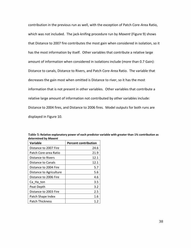
38

contribution in the previous run as well, with the exception of Patch Core-Area Ratio,

which was not included. The jack-knifing procedure run by Maxent (Figure 9) shows

that Distance to 2007 fire contributes the most gain when considered in isolation, so it

has the most information by itself. Other variables that contribute a relative large

amount of information when considered in isolations include (more than 0.7 Gain):

Distance to canals, Distance to Rivers, and Patch Core-Area Ratio. The variable that

decreases the gain most when omitted is Distance to river, so it has the most

information that is not present in other variables. Other variables that contribute a

relative large amount of information not contributed by other variables include:

Distance to 2004 fires, and Distance to 2006 fires. Model outputs for both runs are

displayed in Figure 10.

Table 5: Relative explanatory power of each predictor variable with greater than 1% contribution as determined by Maxent

Variable Percent contribution

Distance to 2007 Fire 24.6

Patch Core-area Ratio 21.9

Distance to Rivers 12.1

Distance to Canals 12.1

Distance to 2004 Fire 5.7

Distance to Agriculture 5.6

Distance to 2006 Fire 4.6

Ca_Ha_ton 3.5

Peat Depth 3.2

Distance to 2003 Fire 2.5

Patch Shape Index 1.6

Patch Thickness 1.2

39

Figure 9. Jackknife test of variable importance produced by Maxent .

40

Figure 10. Maxent Species Distribution Model.

41

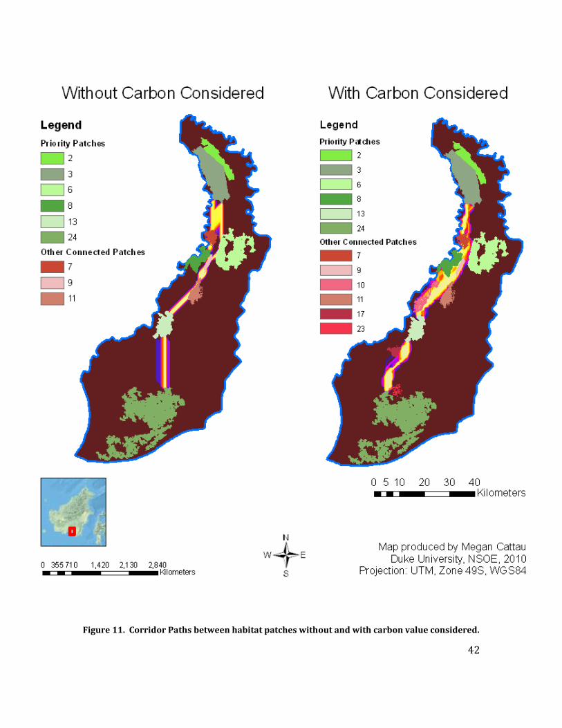
Corridors

The ideal corridor path identified between patches 3 and 13 using the SDM as

the cost surface also included priority patches 6 and 8, as well as patches 7, 9, and 11

(Figure 11). The corridor path between patches 13 and 24 did not include any other

patches. If we consider patch 2 to be connected to patch 3, these corridors would allow

patches 9 patches to be functionally connected in terms of orang-utan dispersal,

increasing the viable population size on Block C from 1,146 individuals to 1,660.

The corridor path identified between patches 3 and 13 using the combined SDM

and carbon value as the cost surface included priority patches 6 and 8 and patches 7, 9,

and 11, just as the analysis completed with the SDM cost surface. However, because

the corridor path followed high-carbon value areas further to the west, it also included

patch 10. Likewise, the corridor path between patches 13 and 24 was located more to

the west than the path found using the SDM cost surface, and so it included two

additional patches, patches 17 and 23. With these three additional patches included in

the functional network, the viable population size on Block C is further increased to

1,788 individuals if the carbon value is considered.

42

Figure 11. Corridor Paths between habitat patches without and with carbon value considered.

43

Discussion

The density, distribution, and abundance of Bornean orang-utans on Block C of

the Former Mega Rice Project was formerly unknown. This information, produced in

this project, will contribute to the body of knowledge concerning this understudied

population and will allow for more accurately focused conservation efforts for these

orang-utans. Additionally, I have identified which existing fragments of habitat are most

vital for the population of orang-utans on Block C and highlighted potential corridor

paths between priority habitat patches. Efforts are currently being made to restore

degraded hydrology and forest on Block C, which will prevent further peatland

oxidation, increase the land’s ability to sequester carbon, retard the detrimental

peatland fires that have been occurring there since the 1990s, and increase the quality

of the forest for the resident population of orang-utans. The analyses completed in this

study will increase the chances that conservation and restoration activities currently

being undertaken on Block C will actually benefit the viability of the orang-utan

population living there by forming a functional network for the population. Additionally,

the incorporation of the carbon value of the land into this study allows for orang-utan

conservation plans that are more economically feasible in this area.

Some additional information would greatly benefit the accuracy of the study.

First, Boehm and Siegert (1999) indicate that intensive ground truth checking is

necessary for an accurate impression of a landscape from satellite data. However, in

this case, I was not able to obtain many ground truth points or an accurate map against

44

which to compare the data that I classified. Additionally, some of the southern area is

distorted by cloud shadow that could not be masked out and, thus, may be incorrectly

classified. However, those details are somewhat negligible in this case, as I was

analyzing peatforest fragments, whose spectral signature was significantly easier to

discern than that of the other land cover classes. Thus, even without ground data or an

accuracy assessment, I feel fairly confident with my success in isolating PSF from other

land cover types. Although the largest fragment, patch 24, was somewhat distorted by

clouds, this did not have a significant effect on the analysis. The masked-out clouds

covering this patch would make the patch appear less condensed than it may be in

reality, but it was still considered one of the priority patches despite this potential

distortion.

Additionally, some of the thresholds chosen for the analysis were somewhat

subjective. For example, the 350 ha threshold selected for minimum orang-utan habitat

patch sizes, although based on range requirements for female orang-utans, did not

consider several additional factors. Specifically, male orang-utan ranges are noted to be

several times larger than female home ranges, but little data is available on the actual

area required. Male ranges are also not exclusive or stable (van Schaik & van Hooff,

1996). Thus, the connectivity of habitat patches becomes especially important for male

dispersal and the resulting genetic variation in individuals and metapopulations across

the landscape. Also, the weighting of the patches based on patch geometry metrics is a

source of uncertainty. Little data is available concerning the response of orang-utan

45

populations to the patch geometry metrics calculated. Patch area was given the most

importance because most conservation planners appreciate the relative importance of

patch area for species protection (Margules and Pressey, 2000). However, other metrics

have been shown to be important determinants of species presence (Helzer and Jelinski,

1999). More research is required in this regard.

If the trends of lowland peatswamp forest loss in Indonesia continue, then the

ability of the area to support orang-utans and other species or to mitigate global climate

change does not appear hopeful. A report by the Indonesian Ministry of Forestry in co-

operation with the European Union states that the world demand for palm oil is

projected to increase twofold by 2020, and that they predict “that by far the largest slice

of this new land will come from within Indonesia where labour and land remain

plentiful. It is inevitable that most new oil palm will be in the wetlands, as the more

'desirable' dry lands of the island are now occupied,” (Sargeant, 2001). If the

agricultural development pressures promised above by this report come to pass, then

the fate of peatswamp forests all over Indonesia appears grim. However, I believe that

the incorporation of the carbon value of the land into land management decisions could

change that. Additionally, in terms of orang-utan conservation specifically, I expect that

the land most suitable for orang-utans will also have the highest value on the carbon

market, as both orang-utan densities and carbon storage are high in areas of deep peat.

This has great implications for the economic feasibility of orang-utan

conservation through the preservation of intact habitat patches and through the

46

establishment of corridors that connect existing populations. More research is needed

concerning the potential to incorporate carbon value into land management decisions

and protection area establishment throughout tropical peatswamp forest areas. Just as

spatially explicit analysis is required for effective species conservation planning, sight-

specific economic valuation of the opportunity cost of conservation will also be

required. Venter et al. (2009b) estimate that payments for REDD at USD 10-33 per

tonne of CO2 (USD 2-16 per tonne if cost-efficient areas are targeted) could feasibly

offset the opportunity costs of forest protection in Kalimantan, Indonesia. On the other

hand, Butler et al. (2009) argue that REDD will not be able to compete with clearing land

for palm oil in Indonesia unless it is incorporated into the compliance market, which

would boost the profitability of forest conservation. Over the next 25 years, 3,750–

5,400 tonnes of CO2 will be emitted for each hectare of peatland developed for oil palm

(Pearce, 2007). Also, if the oil palm is used for biofuel, this will result in 25–36 times

more CO2 emitted from the peatland as would be saved from vehicle emissions (Yule,

2010). There is hope for inaccessible areas like the former Mega-Rice project in

particular, where opportunity costs of conservation still remain relatively low.

Putz and Redfore (2009) mention concerns about carbon-based conservation,

stating that silvicultural interventions intended to boost carbon stock could have

adverse effects on biodiversity. Because biodiversity and other ecosystem services will

not automatically and collaterally benefit from REDD and its preservation of carbon

stocks, it is important to prioritize areas that can have multiple benefits on the ground

47

(Miles and Kapos, 2008). This project has demonstrated how carbon projects can be

planned so that co-benefits are explicitly targeted and benefits are maximized on the

landscape (Venter et al., 2009a). However, for this to be successfully reproduced in

other areas, planning will necessarily be site-specific and spatially explicit.

Additionally, one of the greatest challenges in implementing a biodiversity-

centered approach to carbon market projects will be institutional capacity. There will

need to be support on the regional and national level to ensure that biodiversity is

considered in carbon projects intended for the compliance market. Currently, under the

voluntary framework, CCB Standards and similar standards ensure that the biodiversity

and community livelihood co-benefits are present in a project. For example, the first

REDD project that met the CCBS was the Ulu Masen Project, which protected a large

area of peatswamp forest in Sumatra from being converted into palm oil, while

protecting biodiversity and promoting the livelihood of local communities. To ensure

net positive biodiversity benefits for climate mitigation projects in the compliance

market, this will likely need to be incentivized or required.

This project demonstrates how we might use carbon financing to make possible

not just forest preservation and restoration, but also wildlife protection strategies. The

carbon funding mechanisms of REDD and CDM could be successfully used to preserve

and connect intact forest fragments in single-species or biodiversity conservation

strategies if the co-benefits of carbon projects are appropriately valued.

48

Literature Cited

Aldhous, P. 2004. Land remediation: Borneo is burning. Nature. 432: 144-146. Ancrenaz, M., Gimenez, O., Ambu, L., Ancrenaz, K., Andau, P., Goossens, B., Payne, J.,

Tuuga, A., and Lackman-Ancrenaz, I. 2005. Aerial surveys give new estimates for orang-utans in Sabah, Malaysia. Public Library of Science Biology. 3(1): 30-37.

Ancrenaz, M., Lackman-Ancrenaz, I. and Elahan, H. 2006. Seed spitting and seed

swallowing by wild orang-utans (Pongo pygmaeus morio) in Sabah, Malaysia. Journal of Tropical Biology and Conservation. 2(1): 65-7.

Ancrenaz, M., Marshall, A., Goossens, B., van Schaik, C., Sugardjito, J., Gumal, M. and

Wich, S. 2008. Pongo pygmaeus. In: IUCN 2010. IUCN Red List of Threatened Species. Version 2010.1. <www.iucnredlist.org>. Downloaded on 25 February 2010.

Boehm, H. D. V., and Siegert, F. 1999. Application of Remote Sensing and GIS to survey

and evaluate tropical peat. Kalteng Consultants. International Conference and Workshop on Tropical Peat Swamps, Safeguarding a Global Natural Resource. 27-29 July 1999. Penang, Malaysia.

Buckland, S.T., Anderson, D.R., Burnham, K.P., and Laake, J.L. 1993. Distance

Sampling—Estimating Abundance of Biological Populations. Chapman and Hall, London.

Butler R. A., Koh L. P. and Ghazoul J. 2009. REDD in the red: palm oil could undermine

carbon payment schemes. Conservation Letters. 2: 67-73. Copenhagen Accord, Draft decision. 2009. Conference of the Parties, Fifteenth Session.

1-5. Copenhagen: United Nations Framework Convention on Climate Change.

Crist, E.P. and Kauth, R.J. 1986. The tasseled cap de-mystified. PEERS 52(1):81-86. Elith, J., Graham, C.H., Anderson, R.P., Dudik, M., Ferrier, S., Guisan, A., Hijmans, R.J.,

Huettmann, F., Leathwick, J.R., Lehmann, A., Li, J., Lohmann, L., Loiselle, B.A., Manion, G., Moritz, C., Nakamura, M., Nakazawa, Y., Overton, J.M., Peterson, A.T., Phillips, S., Richardson, K., Schachetti Pereira, R., Schapire, R.E., Soberón, J., Williams, S.E., Wisz, M. and Zimmermann, N.E. 2006. Novel methods improve predictions of species’ distributions from occurrence data. Ecography. 29 (2): 129–151.

49

ESRI. 2008. ArcGIS v.9.3. Redlands, CA. Galdikas, B. M. F. 1988. Orang-utan diet, range and activity at Tanjung Putting, Central

Borneo. International Journal of Primatology. 9:1-35. Goossens, B., Chikhi, L., Ancrenaz, M., Lackman-Ancrenaz, I., Andau, P., and Bruford,

M.W. 2006. Genetic Signature of Anthropogenic Population Collapse in Orang-utans. PLoS Biol 4(2): e25 doi:10.1371/journal.pbio.0040025.

Helzer, C. and Jelinski, D. E. 1999. The Relative Importance of Patch Area and

Perimeter-Area Ratio to Grassland Breeding Birds. Ecological Applications. 9(4): 1448-1458.

Hooijer, A., Silvius, M., Wösten, H. and Page, S. 2006. PEAT-CO2, Assessment of CO2

emissions from drained peatlands in SE Asia. Delft Hydraulics report Q3943. Husson, S. J., Wich, S. A., Marshall, A. J., Dennis, R. D., Ancrenaz, M., Brassey, R., gumal,

M., Hearn, A. J., Meijaard, E., Simorangkir, T., and Singleton, I. 2008. Chapter 6, Orang-utan distribution, density, abundance and impacts of disturbance. In S Wich, S. A., Utami Atmoko, S. S., and Setia, T. M. Orang-utans. 77-97. Oxford Scholarship Online Monographs.

Jaynes, E. T., 1990. Notes on present status and future prospects. In: Grandy Jr., W.T.,

Schick, L.H. (Eds.), Maximum Entropy and Bayesian Methods. Kluwer, Dordrecht, The Netherlands, 1–13.

Margules, C. R. and Pressey, R. L. 2000. Systematic conservation planning. Nature.

405: 243-253.

McCune, B., and Grace, J. B. 2002. Analysis of ecological communities. MjM Software Design, Gleneden Beach, Oregon.

Miles, L. and Kapos, V. 2008. Reducing Greenhouse Gas Emissions from Deforestation

and Forest Degradation: Global Land-Use Implications. Science. 320: 1454-1455. Minnemeyer, S., Boisrobert, L., Stolle, Muliastra, F., Y. I. K. D., Hansen, M., Arunarwati,

B., Prawijiwuri, G., Purwanto, J., and Awaliyan, R. 2009. Interactive Atlas of Indonesia's Forests (CD-ROM). World Resources Institute: Washington, DC.

Morrogh-Bernard, H., Husson, S., Page, S. E., and Rieley, J.O. 2003. Population status of

the Bornean orang-utan (Pongo pygmaeus) in the Sebangau peat swamp forest, Central Kalimantan, Indonesia. Biological Conservation. 110: 141-152.

50

Murray, B., Lubowski, R., and Sohngen, B. 2009. Including International Forest Carbon Incentives in Climate Policy: Understanding the Economics. Duke University and the Nicholas Institute for Environmental Policy Solutions. Durham, NC: Nicholas Institute.

Pearce, F. 2007. Bog barons: Indonesia’s carbon catastrophe. New Scientist. 2632:50–

53. Phillips, S. J., Anderson, R. P., and Schapire, R. E. 2006. Maximum entropy modeling of

species geographic distributions. Ecological Modeling. 190: 231-259. The Provincial Government of Nanggroe Aceh Darussalam, Fauna & Flora International

(FFI), and Carbon Conservation Pty. Ltd. 2007. Reducing Carbon Emissions from Deforestation in the Ulu Masen Ecosystem, Aceh, Indonesia (A Triple-Benefit Project Design Note for CCBA Audit).

Putz, F.E. and Redfore, K.H. 2009. Dangers of carbon-based conservation. Global

Environmental Change. 19: 400-401. Rijksen, H.D. and Meijaard, E. 1999. Our Vanishing Relative: The Status of Wild Orang-

utans at the Close of the Twentieth Century. Dordrecht: Kluwer Academic Publishers.

Sargeant, H.J. 2001. Oil palm agriculture in the wetlands of Sumatra: destruction or

development? Report, Forest fire prevention and control project; Government of Indonesia Ministry of Forestry & European Union.

Singleton I., Wich S. A., Husson S., Stephens S., Utami-Atmoro S. S., Leighton M., Rosen

N., Traylor-Holzer K., Lacy R. C. and Byers O. 2004. Orang-utan Population and Habitat Viability Assessment: Final Report. IUCN/SSC Conservation Breeding Specialist Group. Apple Valley, MN.

Stern, N. 2006. Stern Review of the Economics of Climate Change. Thomas, L., Laake, J.L., Derry, J.F., Buckland, S.T., Borchers, D.L., Burnham, K.P.,

Strindberg, S., Hedley, S.L., Burt, M.L., Marques, F., Pollard, J.H., and Fewster, R.M. 1998. DISTANCE 3.5. Research Unit for Wildlife Population Assessment, University of St Andrews, UK.

van Schaik, C. P. and van Hooff, J.A.R.A.M. 1996. Toward an understanding of the

orang-utan’s social system. From Great Ape Societies. McGrew, W. C., Merchant, L. F., and Nishida, T., eds.

51

Venter, O., Laurance, W.F., Iwamura, T., Wilson, K.A., Fuller, R. A., and Possingham, H.P. 2009a. Harnessing Carbon Payments to Protect Biodiversity. Science. 326: 1368.

Venter O., Meijaard E., Possingham H., Dennis R., Sheil D., Wich S., Hovani L. and Wilson

K. 2009b. Carbon payments as safeguard for threatened tropical mammals Conservation Letters. 2:123-129.

Yeager, C.P. 1999. Fire impacts on vegetational diversity and abundance in Kalimantan,

Indonesia during 1997/1998. WWF-Indonesia report, Jakarta. Yeager, C.P. and Fredriksson, G. 1999. Fire impacts on Primates and other wildlife in

Kalimantan, Indonesia during 1997/1998. WWF-Indonesia report, Jakarta. WWF-Indonesia report, Jakarta.

Yule, C.M. 2010. Loss of biodiversity and ecosystem functioning in Indo-Malayan peat

swamp forests. Biodiversity and Conservation. 19:393-409.

52

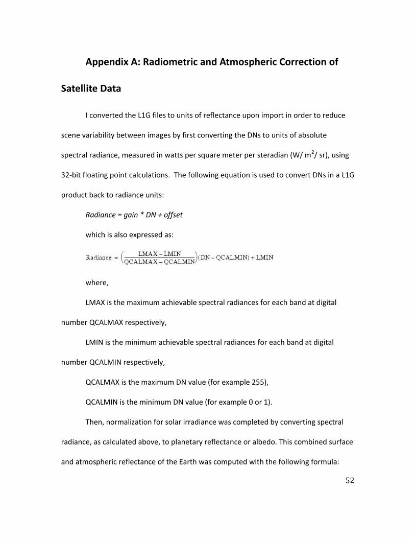
Appendix A: Radiometric and Atmospheric Correction of

Satellite Data

I converted the L1G files to units of reflectance upon import in order to reduce

scene variability between images by first converting the DNs to units of absolute

spectral radiance, measured in watts per square meter per steradian (W/ m2/ sr), using

32-bit floating point calculations. The following equation is used to convert DNs in a L1G

product back to radiance units:

Radiance = gain * DN + offset

which is also expressed as:

where,

LMAX is the maximum achievable spectral radiances for each band at digital

number QCALMAX respectively,

LMIN is the minimum achievable spectral radiances for each band at digital

number QCALMIN respectively,

QCALMAX is the maximum DN value (for example 255),

QCALMIN is the minimum DN value (for example 0 or 1).

Then, normalization for solar irradiance was completed by converting spectral

radiance, as calculated above, to planetary reflectance or albedo. This combined surface

and atmospheric reflectance of the Earth was computed with the following formula:

53

where,

= unitless effect planetary reflectance

= spectral radiance at the sensor's aperture

= Earth-Sun distance in astronomical units

= Mean solar exoatmospheric irradiances

= Solar zenith angle

Current values for are specified in the SUN_ELEVATION record, which was

found in the LPGS_Metadata file.

The value for is calculated by the formula:

54

Appendix B: Variables Used in Maxent Distribution Model

Figure 12. Six of the predictor variables entered into the Maxent model.

55

Figure 13. Five of the predictor variables entered into the Maxent model.