Using Robust Queueing to Expose the Impact of Dependence ...ww2040/WY18OR.pdf · WhittandYou: Dependence in Single-Server Queues OperationsResearch,2018,vol.66,no.1,pp.184–199,©2017INFORMS

This article was downloaded by: [160.39.21.161] On: 04 October 2018, At: 11:40Publisher: Institute for Operations Research and the Management Sciences (INFORMS)INFORMS is located in Maryland, USA

Operations Research

Publication details, including instructions for authors and subscription information:http://pubsonline.informs.org

Using Robust Queueing to Expose the Impact ofDependence in Single-Server QueuesWard Whitt, Wei You

To cite this article:Ward Whitt, Wei You (2018) Using Robust Queueing to Expose the Impact of Dependence in Single-Server Queues. OperationsResearch 66(1):184-199. https://doi.org/10.1287/opre.2017.1649

Full terms and conditions of use: http://pubsonline.informs.org/page/terms-and-conditions

This article may be used only for the purposes of research, teaching, and/or private study. Commercial useor systematic downloading (by robots or other automatic processes) is prohibited without explicit Publisherapproval, unless otherwise noted. For more information, contact [email protected].

The Publisher does not warrant or guarantee the article’s accuracy, completeness, merchantability, fitnessfor a particular purpose, or non-infringement. Descriptions of, or references to, products or publications, orinclusion of an advertisement in this article, neither constitutes nor implies a guarantee, endorsement, orsupport of claims made of that product, publication, or service.

Copyright © 2017, INFORMS

Please scroll down for article—it is on subsequent pages

INFORMS is the largest professional society in the world for professionals in the fields of operations research, managementscience, and analytics.For more information on INFORMS, its publications, membership, or meetings visit http://www.informs.org

http://pubsonline.informs.org

https://doi.org/10.1287/opre.2017.1649

http://pubsonline.informs.org/page/terms-and-conditions

http://www.informs.org

OPERATIONS RESEARCHVol. 66, No. 1, January–February 2018, pp. 184–199

http://pubsonline.informs.org/journal/opre/ ISSN 0030-364X (print), ISSN 1526-5463 (online)

Using Robust Queueing to Expose the Impact of Dependence inSingle-Server QueuesWard Whitt,a Wei Youa

aDepartment of Industrial Engineering and Operations Research, Columbia University, New York, New York 10027Contact: [email protected], http://orcid.org/0000-0003-4298-9964 (WW); [email protected],

http://orcid.org/0000-0003-0844-4194 (WY)

Received: March 4, 2016Revised: October 10, 2016; March 11, 2017Accepted: May 3, 2017Published Online in Articles in Advance:July 31, 2017

Subject Classifications: queues:approximations, networks, algorithmsArea of Review: Stochastic Models


Copyright: © 2017 INFORMS

Abstract. Queueing applications are often complicated by dependence among interar-rival times and service times. Such dependence is common in networks of queues, wherearrivals are departures from other queues or superpositions of such complicated pro-cesses, especially when there are multiple customer classes with class-dependent service-time distributions. We show that the robust queueing approach for single-server queuesproposed in the literature can be extended to yield improved steady-state performanceapproximations in the standard stochastic setting that includes dependence among inter-arrival times and service times.We propose a new functional robust queueing formulationfor the steady-state workload that is exact for the steady-state mean in the M/GI/1 modeland is asymptotically correct in both heavy traffic and light traffic. Simulation experimentsshow that it is effective more generally.

Funding: Support was received from the National Science Foundation [Grants CMMI 1265070 and1634133].

Supplemental Material: The online appendix is available at https://doi.org/10.1287/opre.2017.1649.

Keywords: robust queueing • queueing approximations • dependence among interarrival times and service times • indices of dispersion • heavytraffic • queueing network analyzer

1. IntroductionRobust optimization is proving to be a useful approachto complex optimization problems involving signifi-cant uncertainty; e.g., see Bandi and Bertsimas (2012),Bertsimas et al. (2011), and references therein. In thatcontext, the primary goal is to create an efficient algo-rithm to produce useful, practical solutions that appro-priately capture the essential features of the uncer-tainty. Bandi et al. (2015) have applied this approachto create a robust queueing (RQ) theory, which canbe used to generate performance predictions in com-plex queueing systems, including networks of queuesas well as single queues. Indeed, they construct a fullrobust queueing analyzer (RQNA) to develop rela-tively simple performance descriptions such as those inthe queueing network analyzer (QNA) in Whitt (1983).Our goal in this paper is to make further progress

in the same direction. We do so by introducing newRQ formulations and evaluating their performance.Wetoo want to obtain useful performance descriptions forcomplex queueing networks, but here we only con-sider a single queue. We judge our RQ formulations bytheir ability to efficiently generate useful performanceapproximations for the given stochastic model, whichso far has been mostly intractable.

As emphasized in Bandi and Bertsimas (2012), theintractability is usually due to high dimension, buthigh dimensionality can occur in many different ways.

The RQ in Bandi et al. (2015) emphasizes the highdimension arising when we consider a network ofqueues instead of a single queue. Instead, in this paperwe focus on the high dimension that occurs in a sin-gle queue when there is complex stochastic depen-dence over time in the arrival and service processes.In a sequel, Whitt and You (2016), we focus on thehigh dimension that occurs in a single queue when thedeterministic arrival-rate function is time varying. Forboth problems, we find that the robust optimizationapproach is remarkably effective. Here, we show that,with an appropriate choice of parameters, all our newRQ solutions are asymptotically correct in the heavy-traffic limit. Our most promising new RQ solutionsin (18) and (28) are asymptotically correct in both lighttraffic and heavy traffic. Our simulation experimentsshow that the newRQ solutions provide useful approx-imations more generally.

1.1. Dependence Among Interarrival Times andService Times

Even thoughwe only focus on one single-server queue,ultimately we also want to develop methods that applyto complex networks of queues. We view the presentpaper as an important step in that direction, becauseexperience from applications of QNA has shown that amajor shortcoming is its inability to adequately capturethe dependence among interarrival times and service

184

http://pubsonline.informs.org/journal/opre/

mailto:[email protected]

http://orcid.org/0000-0003-4298-9964

mailto:[email protected]

http://orcid.org/0000-0003-0844-4194


Whitt and You: Dependence in Single-Server QueuesOperations Research, 2018, vol. 66, no. 1, pp. 184–199, ©2017 INFORMS 185

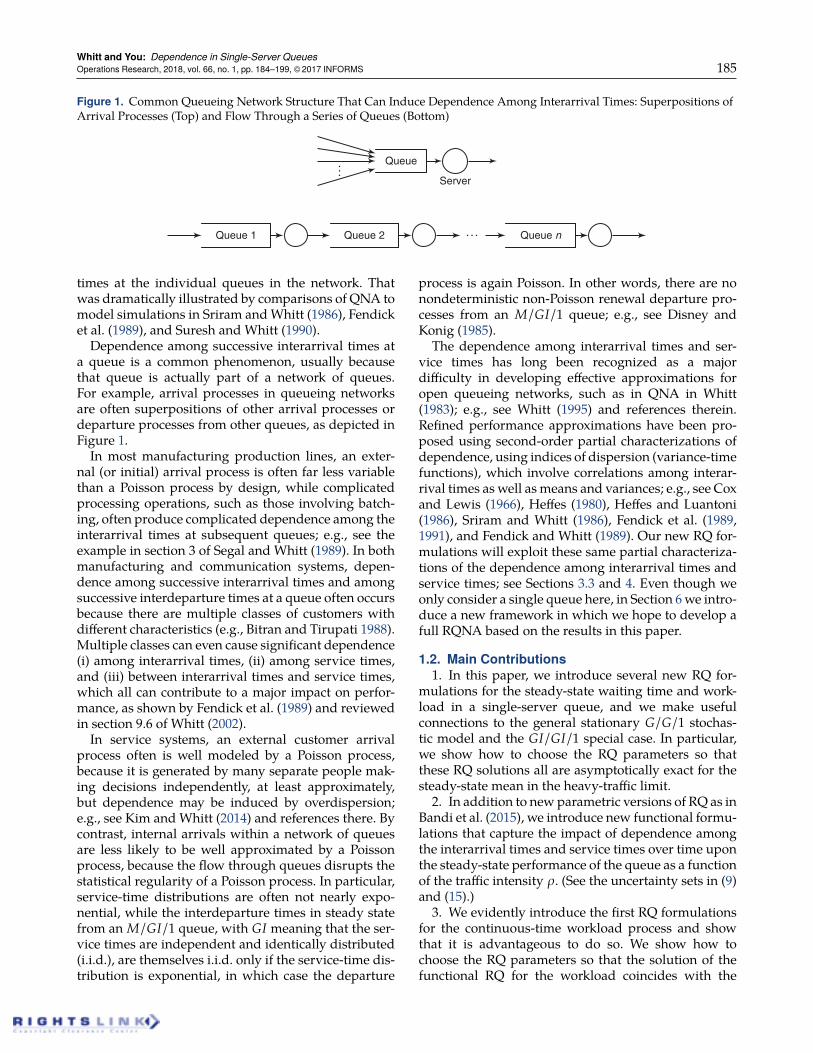
Figure 1. Common Queueing Network Structure That Can Induce Dependence Among Interarrival Times: Superpositions ofArrival Processes (Top) and Flow Through a Series of Queues (Bottom)

Queue

…

Server

Queue 1 Queue 2 Queue n…

times at the individual queues in the network. Thatwas dramatically illustrated by comparisons of QNA tomodel simulations in Sriram andWhitt (1986), Fendicket al. (1989), and Suresh and Whitt (1990).Dependence among successive interarrival times at

a queue is a common phenomenon, usually becausethat queue is actually part of a network of queues.For example, arrival processes in queueing networksare often superpositions of other arrival processes ordeparture processes from other queues, as depicted inFigure 1.

In most manufacturing production lines, an exter-nal (or initial) arrival process is often far less variablethan a Poisson process by design, while complicatedprocessing operations, such as those involving batch-ing, often produce complicated dependence among theinterarrival times at subsequent queues; e.g., see theexample in section 3 of Segal and Whitt (1989). In bothmanufacturing and communication systems, depen-dence among successive interarrival times and amongsuccessive interdeparture times at a queue often occursbecause there are multiple classes of customers withdifferent characteristics (e.g., Bitran and Tirupati 1988).Multiple classes can even cause significant dependence(i) among interarrival times, (ii) among service times,and (iii) between interarrival times and service times,which all can contribute to a major impact on perfor-mance, as shown by Fendick et al. (1989) and reviewedin section 9.6 of Whitt (2002).

In service systems, an external customer arrivalprocess often is well modeled by a Poisson process,because it is generated by many separate people mak-ing decisions independently, at least approximately,but dependence may be induced by overdispersion;e.g., see Kim and Whitt (2014) and references there. Bycontrast, internal arrivals within a network of queuesare less likely to be well approximated by a Poissonprocess, because the flow through queues disrupts thestatistical regularity of a Poisson process. In particular,service-time distributions are often not nearly expo-nential, while the interdeparture times in steady statefrom an M/GI/1 queue, with GI meaning that the ser-vice times are independent and identically distributed(i.i.d.), are themselves i.i.d. only if the service-time dis-tribution is exponential, in which case the departure

process is again Poisson. In other words, there are nonondeterministic non-Poisson renewal departure pro-cesses from an M/GI/1 queue; e.g., see Disney andKonig (1985).

The dependence among interarrival times and ser-vice times has long been recognized as a majordifficulty in developing effective approximations foropen queueing networks, such as in QNA in Whitt(1983); e.g., see Whitt (1995) and references therein.Refined performance approximations have been pro-posed using second-order partial characterizations ofdependence, using indices of dispersion (variance-timefunctions), which involve correlations among interar-rival times as well as means and variances; e.g., see Coxand Lewis (1966), Heffes (1980), Heffes and Luantoni(1986), Sriram and Whitt (1986), Fendick et al. (1989,1991), and Fendick and Whitt (1989). Our new RQ for-mulations will exploit these same partial characteriza-tions of the dependence among interarrival times andservice times; see Sections 3.3 and 4. Even though weonly consider a single queue here, in Section 6we intro-duce a new framework in which we hope to develop afull RQNA based on the results in this paper.

1.2. Main Contributions1. In this paper, we introduce several new RQ for-

mulations for the steady-state waiting time and work-load in a single-server queue, and we make usefulconnections to the general stationary G/G/1 stochas-tic model and the GI/GI/1 special case. In particular,we show how to choose the RQ parameters so thatthese RQ solutions all are asymptotically exact for thesteady-state mean in the heavy-traffic limit.

2. In addition to new parametric versions of RQ as inBandi et al. (2015), we introduce new functional formu-lations that capture the impact of dependence amongthe interarrival times and service times over time uponthe steady-state performance of the queue as a functionof the traffic intensity ρ. (See the uncertainty sets in (9)and (15).)

3. We evidently introduce the first RQ formulationsfor the continuous-time workload process and showthat it is advantageous to do so. We show how tochoose the RQ parameters so that the solution of thefunctional RQ for the workload coincides with the

Whitt and You: Dependence in Single-Server Queues186 Operations Research, 2018, vol. 66, no. 1, pp. 184–199, ©2017 INFORMS

steady-state mean in the M/GI/1 model for all trafficintensities and is simultaneously asymptotically cor-rect in both heavy traffic and light traffic for the generalG/G/1 model, including the dependence.4. We conduct simulation experiments showing that

the new functional RQ for the workload is effectivein exposing the impact of the dependence among theinterarrival times and service times over time upon themean steady-state workload as a function of the trafficintensity.

5. We provide a road map for the application to net-works of queues by introducing a new framework foran RQNAbased on indices of dispersion.We show thatsuch an RQNA is feasible and provide support with asimulation comparison for a series queue network.

1.3. More Related LiteratureMamani et al. (2016) also incorporated dependencewithin a robust optimization formulation for a problemin inventory management (which we might call RI),but otherwise, there is relatively little overlap withthis paper; we discuss the connection in Remark 4.Mamani et al. (2016) point to early RI work by Scarf(1958) and thenMoon and Gallego (1994). The new RQwork is also related to Whitt (1984a), which used opti-mization to study performance approximations usedin QNA. In particular, Whitt (1984a) studied the rangeof possible values for the mean steady-state num-ber in a GI/M/1 queue subject to specified first andsecond moments of the interarrival-time distribution.Klincewicz and Whitt (1984) and Whitt (1984b) con-struct tighter bounds based on additional constraints toenforce a realistic shape on the underlying interarrival-time distribution. This work showed that we can hopeto obtain useful accuracy such as 20% relative error,but that we cannot hope to obtain extraordinarily highaccuracy, such as an only 5% error, given the usual par-tial information based on the first two moments. Andthat is not yet considering the dependence. Ignoringthe dependence can lead to much bigger errors, as inFendick et al. (1989) and section 9.6 of Whitt (2002).

1.4. Organization of the PaperIn Section 2, after reviewing RQ for the steady-statewaiting time in the single-server queue from sections 2and 3.1 of Bandi et al. (2015), we develop an alter-native formulation whose solution coincides with theKingman (1962) bound and is asymptotically correct inheavy traffic. In Section 3 we introduce new parametricand functional RQ formulations for the continuous-timeworkload process and characterize their solutions.In Section 4 we introduce the index of dispersion forwork (IDW) and incorporate it in the RQ. We developclosed-form RQ solutions and show that the func-tional RQ is asymptotically correct in both heavy andlight traffic. In Section 5 we conduct simulation exper-iments for the two network structures in Figure 1.

These experiments demonstrate (i) the strong impactof dependence upon performance and (ii) the valueof the new RQ in capturing the impact of that depen-dence. Finally, in Section 6 we introduce a new frame-work for applying the results in this paper to develop anew RQNA that better captures the dependence. Addi-tional supporting material appears in the e-companion(EC)—in particular, (i) a short summary of the mainpaper; (ii) additional discussion; (iii) additional theo-retical support, including central limit theorems andheavy-traffic limit theorems; (iv) more results for thediscrete-time waiting time and indices of dispersion;and (v) more simulation examples.

2. Robust Queueing for the Steady-StateWaiting Time

We start by reviewing the RQ developed in sections 2and 3.1 of Bandi et al. (2015), which involves sepa-rate uncertainty sets for the arrival times and servicetimes. We then construct an alternative formulationwith a single uncertainty set and show, for the GI/GI/1queue, that a natural version of the RQ solution coin-cides with the Kingman (1962) bound and so is asymp-totically correct in the heavy-traffic limit. We show thatboth formulations provide insight into the relaxationtime for the GI/GI/1 queue, the approximate timerequired to reach steady state.

We use the representation of thewaiting time (beforereceiving service) in a general single-server queuewith unlimited waiting space and the first-come first-served (FCFS) service discipline, without imposing anystochastic assumptions. The waiting time of arrival nsatisfies the Lindley (1952) recursion

Wn � (Wn−1 +Vn−1 −Un−1)+

≡max{Wn−1 +Vn−1 −Un−1 , 0}, (1)

where Vn−1 is the service time of arrival n − 1, Un−1is the interarrival time between arrivals n − 1 and n,and ≡ denotes equality by definition. If we initializethe system by having an arrival 0 finding an emptysystem, then Wn can be represented as the maximumof a sequence of partial sums, using the Loynes (1962)reverse-time construction; i.e.,

Wn � Mn ≡max06k6n

{Sk}, n > 1, (2)

using reverse-time indexing with Sk ≡X1 + · · ·+Xk andXk ≡ Vn−k − Un−k , 1 6 k 6 n, and S0 ≡ 0. (Bandi et al.2015 actually look at the system time, which is the sumof an arrival’s waiting time and service time. Theserepresentations are essentially equivalent.)

If we extend the reverse-time construction indefi-nitely into the past from a fixed present state, then Wn ↑W ≡ supk>0 {Sk} with probability 1 as n→∞, allowing


for the possibility that W might be infinite. For the sta-ble stationary G/G/1 stochastic model with E[Uk]<∞,E[Vk] <∞ and ρ ≡ E[Vk]/E[Uk] < 1, P(W <∞)� 1; e.g.,see Loynes (1962) or section 6.2 of Sigman (1995).Bandi et al. (2015) propose an RQ approximation

for the steady-state waiting time W by performing adeterministic optimization in (2) subject to determinis-tic constraints, where we can ignore the time reversal.Treating the partial sums Sa

k of the interarrival timesUk and the partial sums Ss

k of the service times Vk sep-arately leads to the two uncertainty sets (for W):

Ua ≡ {U ∈ �∞: Sak > kma − ba

√k , k > 0} and

Us� {V ∈ �∞: Ss

k 6 kms + bs

√k , k > 0},

(3)

where U ≡ {Uk : k > 1} and V ≡ {Vk : k > 1} are arbitrarysequences of real numbers in �∞; Sa

k ≡U1 + · · ·+Uk andSs

k ≡ V1 + · · · + Vk , k > 1; S0 ≡ 0; and ma , ms , ba , and bsare parameters to be specified. The constraints in (3)are one-sided because that is what is required to boundthe waiting times above, as we can see from (1) and (2).Thus, the RQ optimization can be expressed as

W ∗ ≡ supU∈Ua

supV∈Us

supk>0{Ss

k − Sak}, (4)

where Sak (Ss

k) is a function of U (V) specified above.Versions of this formulation in (4) and others in thispaper also apply to the transient waiting time Wn , butwe will focus on the steady-state waiting time.Thinking of the general stationary G/G/1 stochas-

tic model, where the distributions of Uk and Vk areindependent of k (but stochastic independence is notassumed), Bandi et al. (2015) assume that ma ≡ E[Uk]and ms ≡ E[Vk] and assume that ma > ms , so that ρ ≡ms/ma < 1. The square-root terms in the constraintsin (3) are motivated by the central limit theorem (CLT).Thinking of the GI/GI/1 model in which the interar-rival timesUk and service timesVk come from indepen-dent sequences of i.i.d. random variables with finitevariances σ2

a and σ2s , the CLT suggests that ba � βaσa and

bs � βsσs for some positive constants βa and βs , perhapswith β� βa � βs .With this choice, these newparametersmeasure the number of standard deviations away fromthe mean in a Gaussian approximation. Bandi et al.(2015) also provide an extension to cover the heavy-tailed case, where finite variances might not exist; then√

k in (3) is replaced by k1/α for 0 < α 6 2, as we wouldexpect from sections 4.5, 8.5, and 9.7 of Whitt (2002),but we will not discuss that extension here.From (1), it is evident that the waiting times depend

on the service times and interarrival times onlythrough their difference Xn . Thus, instead of the twouncertainty sets in (3), we propose the single uncer-tainty set (for each n)

Ux ≡ {X ∈ �∞: Sxk 6 −mk + bx

√k , k > 0}, (5)

where X ≡ {Xk : k > 1} ∈ �∞, Sxk ≡ X1 + · · · + Xk , k > 1,

and S0 ≡ 0, while m and bx are constant parameters tobe specified. To avoid excessively strong constraints forsmall values of k, not justified by the CLT, we couldreplace k in the constraint bounds on the right in (5) bymax {k , kL}, but that lower bound kL has no impact ifchosen appropriately. Combining (2) and (5), we obtainthe alternative RQ optimization

W ∗ ≡ supX∈Ux

supk>0{Sx

k }, (6)

where Sxk is the function of X specified above. The RQ

formulations in (4) and (6) are attractive because theoptimization problems have simple solutions in whichall constraints are satisfied as equalities. That followseasily from the fact that Wn is a nondecreasing (nonin-creasing) function of Vk (of Uk) for all k and n. The sim-ple closed-form solution follows from the triangularstructure of the equations; see section 3.1 of Bandi et al.(2015). The following is a direct extension of theorem 2of Bandi et al. (2015) to include the new RQ formula-tion in (6). The final statement involves an interchangeof suprema, which is justified by Lemma EC.1.

Theorem 1 (RQ Solutions for the Steady-State WaitingTime). The RQ optimizations (4) with ma > ms > 0 and (6)with m > 0 have the solution

W ∗� sup

k>0{−mk + b

√k} 6 sup

x>0{−mx + b

√x}

�−mx∗ + b√

x∗ �b2

4mfor x∗ �

b2

4m2 , (7)

where m � ma −ms > 0. For (4), b ≡ bs + ba; for (6), b ≡ bx .In (7), W ∗ is maximized at one of the integers immediatelyabove or below x∗.

We now establish implications for the GI/GI/1 andgeneral stationary G/G/1 models. To discuss heavy-traffic limits, it is convenient to introduce the trafficintensity ρ as a scaling factor applied to the interar-rival times. Hence, we start with a sequence {(Uk ,Vk)}where E[Uk] � E[Vk] � 1 for all k. Then in model ρ welet the interarrival times be ρ−1Uk , where 0 < ρ < 1.Thus, ms � 1 and ma � ρ

−1, so that m ≡ (1 − ρ)/ρ andW ∗ � b2ρ/4(1− ρ) in (7).Since the CLT underlies the heavy-traffic limit theory

as well as the RQ formulation, it should not be sur-prising that we can make strong connections to heavy-traffic approximations. The new formulation in (6) isattractive because, with a natural choice of the con-stant bx there, it matches the Kingman (1962) boundfor the mean steady-state wait E[W] in the GI/GI/1stochastic model and so is asymptotically correct inheavy traffic, whereas that is not the case for (4) with anatural choice of b. To quantify the variability indepen-dent of the scale, let c2

s ≡Var(V1)/(E[V1])2 �Var(V1) and


c2a ≡Var(U1)/(E[U1])2 � ρ2Var(U1) be the squared coeffi-cients of variation (scvs). Let ≈ denote approximatelyequal, without any precise asymptotic meaning.

Corollary 1 (RQYields the KingmanBound for GI/GI/1).In the setting of (6), if we let bx ≡ β

√Var(X1) and β ≡

√2,

then bx �√

2(c2s + ρ

−2c2a) for the GI/GI/1 model with traffic

intensity ρ, so that

W ∗ ≡W ∗(ρ)� Var(X1)2|E[X1]|

�ρ(c2

s + ρ−2c2

a)2(1− ρ) , (8)

which is the upper bound for E[W] in Theorem 2 of King-man (1962), so that (1 − ρ)W ∗(ρ) → (c2

a + c2s )/2 as ρ ↑ 1,

which supports the heavy-traffic approximation W ∗(ρ) ≈ρ(c2

a + c2s )/2(1−ρ), just as for E[W] in the stochastic model.

On the other hand, in the setting of (4), if we let bs ≡β√Var(V1) and ba ≡ β

√Var(U1), then we obtain b � bs +

ba � β(cs + ρ−1ca) instead of b �

√b2

s + b2a � β

√c2

s + ρ−2c2

a ,as needed.

Remark 1 (The Significance for Approximations). The dif-ference between the RQ solutions for (4) and (6) men-tioned at the end of Corollary 1 can have serious impli-cations for approximations; e.g., if c2

a � c2s � x, then

(c2a + c2

s )/2 � x, while (ca + cs)2/2 � 2x, a factor of 2larger. Hence, if we apply (4) with ba � bs to the simpleM/M/1 queue, one is forced to have a 100% error inheavy traffic. These two coincide onlywhen at least oneof ba and bs is 0 (i.e., in D/GI/1 or GI/D/1 models),and the percentage error is the largest when servicetimes and arrival times have the same variability. For-tunately, robust optimization has flexibility that makesit possible to circumvent the difficulties in the form ofthe optimization in (4). For example, Bandi et al. (2015)use statistical regression in their section 7 to refine theirsolution to (4). Of course, such refinements complicatealgorithms.

These RQ formulations provide insight into the rateof approach to steady state for the GI/GI/1 model, ascaptured by the relaxation time; see section III.7.3 ofCohen (1982) and section XIII.2 of Asmussen (2003).For RQ, steady state is achieved at a fixed time,whereasin the stochastic model, steady state is approachedgradually, with the error |E[Wn]−E[W]| typically beingof order O(n−3/2e−n/r) as n→∞, where r ≡ r(ρ) is calledthe relaxation time. As usual, we say f (t) is O(g(t)) ast→∞, where f and g are positive real-valued func-tions, if f (t)/g(t)→ c as t→∞, where 0 < c <∞.

Corollary 2 (Relaxation Time for the GI/GI/1 Queue).With both (4) and (6), the place where the RQ supremum isattained is x∗(ρ) � O((1− ρ)−2) as ρ ↑ 1, which is the sameorder as the relaxation time in the GI/GI/1 model.

Remark 2 (A Functional RQ to Expose the Impact ofDependence in the G/G/1 Model). The RQ problems

in (4) and (6) can be considered instances of a para-metric RQ, because they depend on the stochasticmodel only through a few parameters—in particular,(ma ,ms , ba , bs) in (4) and (m , bx) in (6). We can exposethe impact of dependence among the interarrival timesand service times on the steady-state waiting time inthe general stationary G/G/1model as a function of thetraffic intensity ρ by introducing a new functional RQformulation. (With the G/G/1 model, we assume sta-tionarity, so that there is awell-defined steady state, butwe allow dependence among the interarrival times andservice times.) To treat the G/G/1 model, we replacethe uncertainty set in (6) by

Uxf ≡ {X: Sx

k 6 E[Sxk ]+ b′x

√Var(Sx

k ), k > 0}. (9)

and similarly for the two constraints in (4). For theGI/GI/1 model, the new uncertainty set (9) is essen-tially equivalent to the previous one in (5), but theycan be very different with dependence. It is significantthat there are CLTs to motivate the form of the con-straints in (9), just as there are in the i.i.d. case under-lying (5). These supporting CLTs are reviewed here inSection EC.5. The CLT supports the spatial scaling by√Var(Sk) instead of

√k, as we show in Section EC.5.3.

Of course, the functional RQ produces a more compli-cated optimization problem, but it is potentially moreuseful, in part because it too can be analyzed. Forbrevity, we discuss this functional RQ for the wait-ing time in the EC because we will next develop sucha functional RQ formulation for the continuous-timeworkload. As discovered in Fendick and Whitt (1989),it is convenient to focus on the steady-state workloadwhen we want to expose the performance impact ofthe dependence among interarrival times and servicetimes.

Remark 3 (Asymptotically Correct in Heavy Traffic for theG/G/1 Model). In Section EC.6.2 we observe that Corol-lary 1 can be extended, with the aid of Sections EC.5and EC.6, to show that both the new parametric RQin (6) and the new functional RQ with uncertainty setin (9) are asymptotically correct in heavy traffic forthe more general stationary G/G/1 model, where weregard {(Uk ,Vk)} as a stationary sequence with thesame mean values, including E[Vk] � 1 and E[Uk] �ρ−1 > 1 for all k. Now we must choose the param-eter bx appropriately to account for the dependenceamong the interarrival times and service times. Justas before, that can be motivated by the CLT, but nowwe need a CLT that accounts for the dependence, asin theorem 4.4.1 and section 9.6 of Whitt (2002); seeSection EC.5.

Remark 4 (Connection to Mamani et al. 2016). At firstglance, the connection to Mamani et al. (2016) may notbe obvious, because we have introduced no explicit


covariances, like what appears in uncertainty set (6) intheir section 2.5. The Lindley recursion in (1) here leadsdirectly to the expression for the steady-state waitingtime in terms of the partial sums Sk in (2), so it isnatural for us to focus on the variances Var(Sk). How-ever, the variances Var(Sk) in our uncertainty set (9)are variances of sums of random variables, which in-cludes covariances of the summands X j when thesesummands are not required to be independent. Asindicated above, our uncertainty sets are motivatedby CLTs, but CLTs without the usual independenceassumption. The second paragraph of section 2.5 inMamani et al. (2016) also mentions CLTs for depen-dent random variables but seems to be suggesting thatthe conditions are too restrictive to be useful. UnlikeMamani et al. (2016), the CLT and the heavy-traffic the-ory play a big role here to expose what properties ofthe model have the greatest impact upon the queueperformance; see Section EC.5.

3. Robust Queueing for theContinuous-Time Workload

We now develop RQ formulations for the continuous-time workload in the single-server queue. We developboth a parametric RQ paralleling (6) and a functionalRQ with an uncertainty set paralleling (9) in Remark 2.

The workload at time t is the amount of unfinishedwork in the system at time t; it is also called the virtualwaiting time because it represents the waiting time ahypothetical arrival would experience at time t. Theworkload is more general than the virtual waiting timebecause it applies to any work-conserving service dis-cipline. We consider the workload primarily because itcan serve as a convenient, more tractable alternative tothe waiting time.We start by developing a reverse-time representa-

tion of the workload process paralleling (2). Then wedevelop both parametric and functional RQ formula-tions and give their solutions, which closely parallelsTheorem 1. We then show that natural versions of bothRQ formulations for the workload are exact for theM/GI/1 model and are asymptotically correct in bothlight traffic and heavy traffic for the general stationaryG/G/1 model.

3.1. The Workload Process and Its Reverse-TimeRepresentation

As before, we start with a sequence {(Uk ,Vk)} of inter-arrival times and service times. The arrival countingprocess can be defined by

A(t) ≡max {k > 1: U1 + · · ·+Uk 6 t} for t >U1 (10)

and A(t) ≡ 0 for 06 t <U1, while the total input of workover [0, t] and the net-input process are, respectively,

Y(t) ≡A(t)∑k�1

Vk and N(t) ≡ Y(t) − t , t > 0, (11)

while the workload (the remainingworkload) at time t,starting empty at time 0, is the reflection map Ψapplied to N ; i.e.,

Z(t)�Ψ(N)(t) ≡N(t) − inf06s6t{N(s)}, t > 0. (12)

As in section 6.3 of Sigman (1995), we again use areverse-time construction to represent the workload ina single-server queue as a supremum, so that the RQoptimization problem becomes a maximization overconstraints expressed in an uncertainty set, just asbefore, but now it is a continuous optimization prob-lem. Using the same notation, but with a new mean-ing, let Z(t) be the workload at time 0 of a systemthat started empty at time −t. Then Z(t) can be repre-sented as

Z(t) ≡ sup06s6t{N(s)}, t > 0, (13)

where N is defined in terms of Y as before, but Y isinterpreted as the total work in service time to enterover the interval [−s , 0]. That is achieved by lettingVk be the kth service time indexed going backwardsfrom time 0 and A(s) counting the number of arrivalsin the interval [−s , 0]. Paralleling the waiting time inSection 2, Z(t) increases monotonically to Z as t→∞.For the stable stationary G/G/1 stochastic queue, Zcorresponds to the steady-state workload and satisfiesP(Z <∞)� 1; see section 6.3 of Sigman (1995).

3.2. Parametric and Functional RQ for theSteady-State Workload

Just as in Section 2, to create appropriate RQ formu-lations for the steady-state workload, it is helpful tohave a reference stochastic model, which can be the sta-ble stationary G/G/1 model, where such a steady-stateworkload is well defined. In discrete time, our formula-tion can be developed by scaling the interarrival times,assuming that E[Vk] � E[Uk] � 1 for all k for a basestationary sequence {(Uk ,Vk)} and introducing ρ byletting the interarrival times be ρ−1Uk when the trafficintensity is ρ, 0 < ρ < 1. (That was done in Section 2,right after Theorem 1.) Now, in continuous time, we doessentially the same, but now we need to work withcontinuous-time stationarity instead of discrete-timestationarity; e.g., see Sigman (1995). Hence, we assumethat there is a base stationary process {(A(t),Y(t)):t > 0} with E[A(t)] � E[Y(t)] � t for all t > 0 and intro-duce ρ by simple scaling via

Aρ(t) ≡A(ρt) and Yρ(t) ≡ Y(ρt),t > 0 and 0 < ρ < 1, (14)

which implies that E[Aρ(t)]�E[Yρ(t)]� ρt for all t > 0.Then Nρ(t) ≡ Yρ(t) − t and Zρ(t) �Ψ(Yρ)(t), t > 0, justas in (11) and (12). With the reverse-time construction,


Zρ(t) can be expressed as a supremumover the interval[0, t], just as in (13).Within that scaling framework, the natural paramet-

ric and functional (see Remark 2) uncertainty sets forthe steady-state workload are, respectively,

Upρ≡{Nρ: �+→�: Nρ(s)6−(1−ρ)s+bp

√s , s>0} and

Uρ≡Ufρ≡

{Nρ: �+→�: Nρ(s)6E[Nρ(s)]

+b f

√Var(Nρ(s)), s>0

},

�{

Nρ: �+→�: Nρ(s)6−(1−ρ)s+b f

√Var(Nρ(s)), s>0

},(15)

where we regard Nρ ≡ {Nρ(s): 0 6 s 6 t} as an arbi-trary real-valued function on �+ ≡ [0,∞), while weregard {Nρ(s): s > 0} as the underlying stochastic pro-cess and {Var(Nρ(s)): s > 0} � {Var(Yρ(s)): s > 0} as itsvariance-time function, which can be either calculatedfor a stochastic model or estimated from simulationor system data; see Section 4.3. In (15), bp and b f areparameters to be specified.

Remark 5 (Choosing the Parameters bp and b f ). The pa-rameters bp and b f in (15) add a degree of freedomin the algorithm, but some choices lead to asymptoti-cally correct values of the steady-state mean workload,while others do not. On the basis of Corollary 3 below,we will let b �

√2 after this section.

Paralleling Section 2, the associated parametric andfunctional RQ formulations are ,

Z∗p , ρ ≡ supNρ∈U

pρ

sups>0{Nρ(t)},

Z∗ρ ≡ Z∗f , ρ ≡ supNρ∈U

fρ

sups>0{Nρ(t)}.

(16)

As in Section 2, our RQ formulations in (16) are moti-vated by a CLT but here for Yρ(t) (which implies anassociated CLT for Nρ(t)), which we review in Sec-tion EC.5; in particular, see (EC.14) and (EC.16). Thesame reasoning as before yields the following analogof Theorem 1. The proof can be found in Section EC.7.

Theorem 2 (RQSolutions for theWorkload).The solutionsof the RQ optimization problems in (16) are

Z∗p , ρ �−(1− ρ)x∗ + bp

√x∗ �

b2p

4|1− ρ |

for x∗ ≡ x∗(ρ)�b2

p

4(1− ρ)2 (17)

and

Z∗ρ ≡ Z∗f , ρ � sups>0

{− (1− ρ)s + b f

√Var(Yρ(s))

}. (18)

We immediately obtain the following corollary,which states that the RQ formulation in (16) yieldsthe exact mean steady-state workload for the M/GI/1model.

Corollary 3 (Exact for M/GI/1). For the M/GI/1 model,the total input process {Yρ(t): t > 0} in (14) is a com-pound Poisson process with E[Yρ(t)]� ρt and Var(Yρ(t))�ρt(c2

s + 1), so that Z∗f , ρ � Z∗p , ρ if b2p � b2

f ρ(c2s + c2

a). If, inaddition, b f ≡

√2, then

Z∗p , ρ � Z∗f , ρ �ρ(c2

s + c2a)

2(1− ρ) � E[Zρ], (19)

where E[Zρ] is the mean steady-state workload in theM/GI/1 model with traffic intensity ρ.

This corollary suggests a natural choice of b f in (15).From now on, we assume that b f �

√2 unless otherwise

stated.

3.3. The Variance-Time Function for theTotal Input Process

For further progress, we focus on the variance-timefunction Var(Yρ(t)) in (18). As regularity conditions forY(t), we assume that V(t) ≡ Vρ(t) ≡ Var(Yρ(t)) is dif-ferentiable with derivative ÛV(t) having finite positivelimits as t→∞ and t→ 0; i.e.,

ÛV(t)→ σ2Y as t→∞ and

ÛV(t)→ ÛV(0) > 0 as t→ 0(20)

for an appropriate constant σ2Y . These assumptions are

known to be reasonable; see section 4.5 of Cox andLewis (1966), Fendick andWhitt (1989), and Section 4.3.

A common case in models for applications is to havepositive dependence in the input process Y, whichholds if

Cov(Y(t2) −Y(t1),Y(t4) −Y(t3)) > 0for all 0 6 t1 < t2 6 t3 < t4. (21)

Negative dependence holds if the inequality is re-versed. These are strict if the inequality is a strictinequality. From (17) and (18) of section 4.5 in Coxand Lewis (1966), which is restated in (48) and (49)of Fendick and Whitt (1989), with positive (negative)dependence, under appropriate regularity conditions,ÛV(t) > 0 and ÜV(t) > (6)0.Remark 6 (Example of Negative Dependence).Negativedependence in Y occurs if greater input in one inter-val tends to imply less input in another interval. Suchnegative dependence occurs when there is a specifiednumber of arrivals in a long time interval, as in the∆(i)/GI/1 model, where the arrival times (not interar-rival times) are i.i.d. over an interval; see Honnappaet al. (2015). This phenomenon can also occur in


queues with arrivals by appointment, where thereare i.i.d. deviations about deterministic appointmenttimes; e.g., see Kim et al. (2017).

Theorem 3 (RQ Exposing the Impact of the Depen-dence). Consider the functional RQ optimization for thesteady-state workload in the general stationary G/G/1 queuewith ρ < 1 formulated in (16) and solved in (18). Assumethat (20) holds for the variance-time function V(t) ≡Vρ(t) ≡Var(Yρ(t)).(a) For each ρ, 0 < ρ < 1, there exists (possibly not

unique) x∗ ≡ x∗(ρ), such that a finite maximum is attainedat x∗ for all t > x∗. In addition, 0 < x∗ <∞ and x∗ satisfiesthe equation

(1− ρ)� Ûh(x), where h(x) ≡ b′z√

V(x). (22)

The time x∗ is unique if h(x) is strictly concave orstrictly convex—i.e., if Ûh(x) is strictly increasing or strictlydecreasing.(b) If there is positive (negative) dependence, as in (21)

(with sign reversed), the variance function V(x) is convex(concave), so that the function h(x) ≡

√V(x) is concave.

Moreover, a strict inequality is inherited. Thus, there existsa unique solution to the RQ if there is strict positive depen-dence or strict negative dependence. Moreover, the optimaltime x∗(ρ) is strictly increasing in ρ, approaching 1 as ρ ↑1,so that Z∗ρ→ ÛV(∞)� Iw(∞)� σ2

Y as ρ ↑ 1.

Proof. The inequalities can be satisfied as equalitiesjust as before. There are finite values s0 such that√

V(s)6√

2σ2Y s for all s > s0 by virtue of the limit in (20).

(Also see (EC.1) and (EC.12).) That shows that the opti-mization can be regarded as being over closed boundedintervals. The assumed differentiability of V impliesthat it is continuous, which implies that the supremumis attained over the compact interval. Because ÛV(x) →ÛV(0) > 0, we see that there exists a small s′ such that

−(1− ρ)s + b′z√

V(s) > −(1− ρ)s + b′z√

s ÛV(0)/2 > 0for all s 6 s′.

As a consequence, themaximum in (18)must be strictlypositive andmust be attained at a strictly positive time.The results for

√V(x) with positive dependence fol-

low from convexity properties of compositions. First,with positive dependence, −

√V(x) is a convex func-

tion of an increasing convex function and thus convexso that

√V(x) is concave. Second, with negative depen-

dence, we have V > 0, ÛV(t) > 0 and ÜV(t) 6 (6)0. Thus,by direct differentiation,

Üh(x)� 1√V(x)

( ÜV(x)2 −

ÛV(x)4V(x)

)6 0,

with strictness implying a strict inequality. �

4. The Indices of Dispersion forCounts and Work

The workload process is convenient not only becauseit leads to the continuous RQ optimization problemin (16) with a solution in (18) but also because thework-load process scales with ρ in a more elementary waythan the waiting times, as indicated in (14). By con-trast, the scaling of the waiting times (specified in thefirst paragraph after Theorem 1) is more complicatedbecause the interarrival times are scaled with ρ but theservice times are not.

It is also convenient to relate the variances of thearrival counting process A(s) and the cumulativework input process Y(s) to associated continuous-timeindices of dispersion, studied in Fendick and Whitt(1989) and Fendick et al. (1991). We define the indexof dispersion for counts (IDC) associated with the rate-1arrival process A as in section 4.5 of Cox and Lewis(1966) by

Ia(t) ≡Var(A(t))E[A(t)] �

Var(A(t))t

, t > 0 (23)

and the index of dispersion for work (IDW) associatedwith the rate 1 cumulative input process Y by

Iw(t) ≡Var(Y(t))

E[V1]E[Y(t)]�

V(t)t, t > 0. (24)

Clearly, these indices of dispersion are just scaled ver-sions of the associated variance functions, but they areimportant for understanding because they expose thevariability over time, independent of the scale. The rea-son for using these indices of dispersion is just likethe reason for using the scvs (introduced before Corol-lary 1) instead of the variances. More generally, thisis consistent with the well-established practice of care-fully focusing on units in physics and engineering.

Fendick and Whitt (1989) show that the IDW Iw isintimately related to a scaled mean workload c2

Z(ρ),which can be defined by comparing to what it wouldbe in the associated M/D/1 model; i.e.,

c2Z(ρ) ≡

E[Zρ]E[Zρ; M/D/1] �

2(1− ρ)E[Zρ]E[V1]ρ

�2(1− ρ)E[Zρ]

ρ. (25)

The normalization in (25) exposes the impact of vari-ability separately from the traffic intensity. Hence, itshould not be surprising that c2

Z(ρ) should be relatedto the IDW. Indeed, under regularity conditions (seeSection EC.5.5), the following finite positive limits existand are equal:

limt→∞{Iw(t)} ≡ Iw(∞)� σ2

Y � c2Z(1)≡ lim

ρ→1{c2

Z(ρ)}, and

limt→0{Iw(t)} ≡ Iw(0)�1+ c2

s � c2Z(0)≡ lim

ρ→0{c2

Z(ρ)}(26)


for c2s ≡Var(V1)/E[V1]2 and c2

Y in (20) and (EC.7). Thelimits for Iw above and the differentiability of Iw followfrom the assumed differentiability for V(t) and limitsin (20). For t→0 and ρ→0, see section IV.A of Fendickand Whitt (1989).The challenge is to relate c2

Z(ρ) to the IDW Iw(t) for0< ρ < 1 and t > 0. As observed by Fendick and Whitt(1989), a simple connection would be c2

Z(ρ) ≈ Iw(tρ)for some increasing function tρ, reflecting that the im-pact of the dependence among the interarrival timesand service times has impact on the performance of aqueue over some time interval [0, tρ], where tρ shouldincrease as ρ increases. The extreme cases are sup-ported by (26), but we want more information aboutthe cases in between.

4.1. Robust Queueing with the IDWTo obtain more information, RQ can help. As a firststep, we express the solution in (18) as

Z∗ρ � sups>0

{−(1−ρ)s + b f

√Var(Yρ(s))

}� sup

s>0

{−(1−ρ)s + b f

√ρsIw(ρs)

}, (27)

using (24). Making the change of variables x ≡ ρs, wecan write

Z∗ρ � supx>0

{−(1−ρ)x/ρ+ b f

√xIw(x)

}. (28)

Clearly, from an algorithmic perspective, (28) is essen-tially the same as (18) and (27), but (28) is helpfulfor developing approximations and insights, includ-ing supporting theory. Our algorithm will exploit theone-dimensional optimization problem in (28), whichis easy to solve given the IDW Iw(x). We will discussmethods of estimating and calculating IDW in Sec-tions 4.3 and 6.To further relate the RQ solution in (28) to the steady-

state workload in the G/G/1 queue, we define an RQanalog of the normalized mean workload in (25)—inparticular,

c2Z∗(ρ)≡

2(1−ρ)Z∗ρρ

. (29)

The RQ approach allows us to establish versions of thevariability fixed-point equation suggested in (9), (15),and (127) of Fendick and Whitt (1989).

Theorem 4 (Restatement of Theorem 2 in Terms of theIDW). Any optimal solution of the RQ in (28) is attained ats∗(ρ)≡ x∗/ρ, where x∗≡ x∗(ρ) satisfies the equation

x∗�b2

f ρ2Iw(x∗)

4(1−ρ)2

(1+

x∗ ÛIw(x∗)Iw(x∗)

)2

(30)

for b f in (18). The associated RQ optimal workload in (28)can be expressed as

Z∗ρ �b2

f ρIw(x∗)4(1−ρ)

(1−

(x∗ ÛIw(x∗)Iw(x∗)

)2), (31)

which is a valid nonnegative solution provided thatx∗ ÛIw(x∗)6 Iw(x∗). If b f �

√2, then the associated scaled RQ

workload satisfies

c2Z∗(ρ)� Iw(x∗)

(1−

(x∗ ÛIw(x∗)Iw(x∗)

)2). (32)

Proof. Note that xIw(x) � V(x). Because we haveassumed that V(x) is differentiable, so too is Iw . Weobtain (30) by differentiating with respect to x in (28)and setting the derivative equal to 0. After substitut-ing (30) into (28), algebra yields (31). The limits in (20)imply that x∗ ÛIw(x∗)→0 and Iw(x∗)→ Iw(∞) as ρ→1. �

Given that x ÛIw(x)→ 0 as x→∞, if b f �√

2, then it isnatural to consider the approximation

x∗(ρ)≈ρ2

2(1−ρ)2 Iw(x∗(ρ)) so that

Z∗ρ ≈ρIw(x∗(ρ))

2(1−ρ) and c2Z∗(ρ)� Iw(x∗(ρ)).

(33)

The first equation in (33) is a variability fixed-pointequation of the form in suggested in (15) of Fendickand Whitt (1989).

4.2. Heavy-Traffic and Light-Traffic LimitsThe following result shows the great advantage ofdoing RQ with (i) the continuous-time workload and(ii) the functional version of the RQ in (28). A proof isgiven in Section EC.7.

Theorem 5 (Heavy-Traffic and Light-Traffic Limits). Underthe regularity conditions assumed for the IDW Iw(t), if b f ≡√

2, then the functional RQ solution in (28) is an asymptot-ically correct characterization of steady-state mean workloadboth in heavy traffic (as ρ ↑ 1) and light traffic (as ρ ↓ 0).Specifically, we have the following supplement to (26):

limρ↑1

c2Z∗(ρ)� Iw(∞)� lim

ρ↑1c2

Z(ρ) and

limρ↓0

c2Z∗(ρ)� Iw(0)� lim

ρ↓0c2

Z(ρ).(34)

Remark 7. Theorem 5 greatly generalizes results inTheorem 3(b) with both light and heavy traffic ad-dressed in the general case beyond positive or negativecorrelations. We also note that the parametric RQ solu-tion can be made correct in heavy traffic or in lighttraffic, as above, by choosing the parameter bp appro-priately, but both cannot be achieved simultaneouslyunless Iw(∞)� Iw(0).


4.3. Estimating and Calculating the IDWFor applications, it is significant that the IDW Iw(t)used in Section 4 can readily be estimated from datafrom system measurements or simulation and calcu-lated in a wide class of stochastic models. The time-dependent variance functions can be estimated fromthe time-dependent first and second moment func-tions, as discussed in section III.B of Fendick et al.(1991). Calculation depends on the specific modelstructure.4.3.1. The G/GI/1 Model. If the service times are i.i.d.with a general distribution having mean τ and scv c2

sand are independent of a general stationary arrival pro-cess, then as indicated in (58) and (59) in section III.Eof Fendick and Whitt (1989),

Iw(t)� c2s + Ia(t), t > 0, (35)

where c2s is the scv of a service time and Ia is the IDC

of the general arrival process.4.3.2. TheMulticlass

∑i(Gi/Gi)/1 Model. As indicated

in (56) and (57) in section III.E of Fendick and Whitt(1989), if the input comes from independent sources,each with their own arrival process and service times,then the overall IDC and IDW are revealing functionsof the component ones. Let λi be the arrival rate, letτi be the mean service time of class i, and let ρi ≡λiτi be the traffic intensity for class i with λ ≡∑

i λi ,τ ≡ ∑

i(λi/λ)τi � 1 so that ρ � λ. With our scalingconventions,

Ia(λt)≡Var(A(t))E[A(t)] �

∑i Var(Ai(t))

λt�∑

i

λi

λIa , i(λi t) (36)

and

Iw(λt)≡ Var(X(t))τE[X(t)] �

∑i Vi(t)ρt

�∑

i

ρiτi

ρτIw , i(λi t)

for all t > 0. (37)

From (36) and (37), we see that Ia and Iw are convexcombinations of the component Ia , i and Iw , i modifiedby additional time scaling.4.3.3. TheMulticlass

∑i Gi/GI/1 Model. An important

special case of Section 4.3.2 arising in open queueingnetworks is the ∑

i Gi/GI/1 model in which there aremultiple general arrival streams coming to a queuewhere all arrivals experience common i.i.d. servicetimes. We can combine (35) and (36) to get the expres-sion for the IDW,

Iw(λt)≡ Ia(λt)+ c2s , t > 0, (38)

where Ia(λt) is given by (36). Of course, if all thecomponent arrival streams are Poisson processes, thenIa(λt)�1 for all t > 0, but otherwise, the IDC Ia(λt) canbe quite complicated.

4.3.4. The Balanced∑

i Gi/GI/1 Model. An importantspecial case of Section 4.3.3 is the balanced ∑

i Gi/GI/1model in which the arrival process is the superposi-tion of n i.i.d. non-Poisson processes each with rateρ/n, so that the overall arrival rate is ρ, and asymptoticvariability parameter is c2

a . From the results above, weobtain

Ia ,n(ρt)� Ia ,1(ρt/n) and Iw ,n(ρt)� Iw ,1(ρt/n),t > 0, (39)

so that the superposition IDI and IDWdiffer from thoseof a single-component process only by the time scaling,but that time scaling involves both n and ρ.As discussed in section 9.8 of Whitt (2002), this

model is known to have complex behavior as a func-tion of n and ρ, so that RQ may be helpful. In partic-ular, under regularity conditions, (i) the superpositionarrival process is known to be non-Poisson and nonre-newal, unless the component arrival streams are Pois-son. (ii) If we let n→∞ but keep the total rate fixed,then the superposition process approaches a Poissonprocess. (iii) However, for any n, no matter how large,if we let t→∞, then the superposition process obeysthe same CLT as a single component arrival processand so has asymptotic variability parameter c2

a . Thus,we have Ia(0)�1 and Ia(∞)� c2

a , but Ia(t) depends on nand ρ in a complicated way for 0< t <∞.

As shown in Whitt (1985), important insight can begained by considering the joint limit as n ↑∞ and ρ↑1.It turns out the asymptotic behavior depends on thelimit of n(1−ρ)2. The separate limits occur if that limitis either infinite or zero. A complex interaction occursat finite limits. We will show that RQ provides impor-tant insight when we conduct simulation experimentsfor this model in Section 5.1.4.3.5. The IDCs for Common Arrival Processes. Thetwo previous subsections show that for a large class ofmodels the main complicating feature is the IDC of thearrival process from a single source. The only reallysimple case is a Poisson arrival process with rate λ.Then Ia(t)�1 for all t > 0. A compound (batch) Poissonprocess is also elementary because the process Y hasindependent increments; then the arrival process itselfis equivalent to M/GI source. However, for a large classofmodels, the variance Var(A(t)) and thus the IDC Ia(t)can either be calculated directly or be characterized viatheir Laplace transforms and thus calculated by invert-ing those transforms and approximated by performingasymptotic analysis. For all models, we assume that theprocesses A and Y have stationary increments.

An important case for A is the renewal process; tohave stationary increments, we assume that it is theequilibrium renewal process, as in section 3.5 of Ross(1996). Then Var(A(t)) can be expressed in terms ofthe renewal function, which in turn can be related


to the interarrival-time distribution and its transform.The explicit formulas for renewal processes appear in(14), (16), and (18) in section 4.5 of Cox (1962). Therequired numerical transform inversion for the renewalfunction is discussed in section 13 of Abate and Whitt(1992). The hyperexponential (H2) and Erlang (E2) spe-cial cases are described in section III.G of Fendick andWhitt (1989).It is also possible to carry out similar analyses for

muchmore complicated arrival processes. Neuts (1989)applies matrix-analytic methods to give explicit rep-resentations of the variance Var(A(t)) for the versatileMarkovian point process or Neuts process; see sec-tion 5.4, especially theorem 5.4.1. Explicit formulas forthe Markov-modulated Poisson process are given onpages 287–289.All of these explicit formulas above have the asymp-

totic form

Var(A(t))� σ2At + ζ+O(e−γt) as t→∞.

5. Simulation ComparisonsWe illustrate how the new RQ approach can be usedwith system data from queueing networks by apply-ing simulation to analyze two common but challeng-ing network structures in Figure 1: (i) a queue with asuperposition arrival process and (ii) several queuesin series. The specific examples are chosen to capturea known source of difficulty: there is complex depen-dence in the arrival process to the queue, so that therelevant variability parameter of the arrival process atthe queue can depend strongly on the traffic inten-sity of that queue, as discussed in Whitt (1995). OurRQ approximations are obtained by applying (28) afterestimating the IDC and applying (35).

Figure 2. (Color online) Left: A Comparison Between Simulation Estimates of the Normalized Mean Workload c2Z(ρ) in (25)

and Its Approximation c2Z∗ (ρ) in (29) as a Function of ρ for the ∑n

i GIi/H2/1 Model with c2s �2 and a Superposition of n i.i.d.

Lognormal Renewal Arrival Processes for n �10 and c2a �10; Right: Graphical RQ Solution Showing h(x)≡

√2xIw(x) and the

Tangent Line with Slope (1−ρ)/ρ at x∗≈482 for ρ�0.9 and at x∗≈17 for 0.7, as Dictated by (22)

Traffic intensity

0

2

4

6

8

10

12

Nor

mal

ized

wor

kloa

d

RQSimulation

0 0.2 0.4 0.6 0.8 1.0 0 100 200 300 400 500 600

Time

0

20

40

60

80

100

120

h(x)

� = 0.7� = 0.9

5.1. A Queue with a Superposition Arrival ProcessWe start by looking at an example of a balanced∑

i Gi/GI/1 model from Section 4.3.4, where (39) can beapplied. Let the rate 1 arrival process A be the superpo-sition of n � 10 i.i.d. renewal processes, each with rate1/n, where the times between renewals have a lognor-mal distribution with mean n and scv c2

a � 10. Let theservice-time distribution be hyperexponential (H2), amixture of two exponential distributions with mean 1,c2

s � 2, and balanced means as on page 137 of Whitt(1982). Then (39) and (26) imply that the IDW has lim-its Iw(0)� 1+ c2

s � 3 and Iw(∞)� c2a + c2

s � 12, so that theIDW is not nearly constant.

The left panel of Figure 2 shows a comparison be-tween the simulation estimate of the normalized work-load c2

Z(ρ) in (25) and the approximation c2Z∗(ρ) in (29)

for this example. We make two important observa-tions: (i) the normalized mean workload c2

Z(ρ) in (25)as a function of ρ is not nearly constant, and (ii) thereis a close agreement between the RQ approximationc2

Z∗(ρ) in (29) and the direct simulation estimate; theclose agreement for all traffic intensities is striking. It isimportant to note that the parametric RQ approxima-tions produce constant approximations and so cannotbe simultaneously good for all traffic intensities.

For this example, we see that c2Z(ρ) ≈ 3 for ρ 6 0.5,

which is consistent with the Poisson approximation forthe arrival process and the associated M/G/1 queue,where c2

Z(ρ)�3 for all ρ, but the normalized workloadincreases steadily to 12 after ρ � 0.5, as explained insection 9.8 of Whitt (2002).

The estimates for Figure 2 were obtained for ρ over agrid of 99 values, evenly spaced between 0.01 and 0.99.Similarly, the RQ optimization was performed using(28) with a discrete-time estimate of the IDW. By doing


multiple runs, we ensured that the statistical variationwas not an issue. For the main simulation of the arrivalprocess and the queuewe used 5×106 replications, dis-carding a large initial portion of the workload processto ensure that the system is approximately in steadystate. (The component renewal arrival processes thuscan be regarded as equilibrium renewal processes, asin section 3.5 of Ross 1996.) We let the run length andamount discarded be increasing in ρ, as dictated byWhitt (1989). We provide additional details about oursimulation methodology in the appendix.

5.2. A Series of Ten QueuesThis second example is a variant of examples in SureshandWhitt (1990), exposing the complex impact of vari-ability on performance in a series of queues if theexternal arrival process and service times at a pre-vious queue have very different levels of variability.This example has 10 single-server queues in series.The external arrival process is a rate 1 renewal pro-cess with H2 interarrival times having c2

a � 5. The firstnine queues all have Erlang service times with c2

a � 0.5denoted by E2, i.e., the sum of two i.i.d. exponentialrandom variables. The first eight queues have meanservice time and thus traffic intensity 0.6, while theninth queue has mean service time and thus trafficintensity 0.95. The last (10th) queue has an exponentialservice-time distribution with mean and traffic inten-sity ρ; we explore the impact of ρ on the performanceof that last queue.The Erlang services act to smooth the arrival pro-

cess at the last queue. Thus, for sufficiently low trafficintensities ρ at the last queue, the last queue shouldbehave essentially the same as a E2/M/1 queue, whichhas c2

a �0.5, but as ρ increases, the arrival process at the

Figure 3. (Color online) A Comparison Between Simulation Estimates of the Normalized Mean Workload c2Z(ρ) in (25) at the

Last Queue of the 10 Queues in Series with Highly Variable External Arrival Process, but Low-Variability Service Times, as aFunction of the Mean Service Time and Traffic Intensity ρ There with the Corresponding Value in the E2/M/1 Queue (Left)and with the RQ Approximation c2

Z∗ (ρ) in (29) (Right)

0

1

2

3

4

5

6

Nor

mal

ized

wor

kloa

d

0

1

2

3

4

5

6

Nor

mal

ized

wor

kloa

d

Queues in seriesE2/M/1

RQSimulation

Traffic intensity

0 0.2 0.4 0.6 0.8 1.0

Traffic intensity

0 0.2 0.4 0.6 0.8 1.0

last queue should inherit the variability of the externalarrival process and behave like an H2/M/1 queue withscv c2

a � 5. This behavior is substantiated by Figure 3,which compares simulation estimates of the normal-ized mean workload c2

Z(ρ) in (25) at the last queue of10 queues in series as a function of the mean servicetime and traffic intensity ρ there with the correspond-ing values in the E2/M/1 queue (left panel) and withthe RQ approximation c2

Z∗(ρ) in (29) (right panel). Theleft panel of Figure 3 shows that the last queue behaveslike a E2/M/1 queue for all traffic intensities 6 0.8 butthen starts behavingmore like an H2/M/1 queue as thetraffic intensity approaches the value 0.95 at the ninthqueue. The right panel of Figure 3 shows that RQ suc-cessfully captures this phenomenon and provides anaccurate approximation for all ρ.

To elaborate on this series-queue example, we showthe IDW for the last queue in Figure 4. The plotshows the IDW assuming continuous-time stationar-ity (which we use) together with the plot using thediscrete-time Palm stationarity (see Sigman 1995) overthe long interval [10−2 ,105] in log scale. The good per-formance in Figure 3 for small values of ρ depends onusing the proper (continuous-time) version.

We conclude this example by illustrating the dis-crete-time approach for approximating the expectedsteady-state waiting time E[W] using the RQ optimiza-tion in (6) with uncertainty set in (9). Figure 5 is the dis-crete analog of Figure 3. Figure 5 compares simulationestimates of the normalized mean waiting time c2

W (ρ),defined just as in (25), at the last queue of 10 queues inseries as a function of the mean service time and traf-fic intensity ρ there with the corresponding values inthe E2/M/1 queue (left) and with the RQ approxima-tion c2

W∗(ρ), defined just as in (29). Figures 5 and 3 look


Figure 4. (Color online) The IDW at the Last Queue Overthe Interval [10−2 ,105] in Log Scale

10–2 100 102 104

Time

0

1

2

3

4

5

6

IDW

PalmStationary

Note. The continuous-time stationary version used for RQ with theworkload is contrasted with the discrete-time Palm version.

similar, except that there is a significant difference forsmall values of ρ. In general, we do not expect RQ tobe effective for extremely low ρ because (i) the CLT isnot appropriate for only a few summands, and (ii) themean waiting time is known to depend on other fac-tors when ρ is small. The mean waiting time and meanworkload actually are quite different in light traffic; seesection IV.A of Fendick andWhitt (1989). As explainedthere, the mean workload tends to be more robust tomodel detail.

Figure 5. (Color online) Contrasting the Discrete-Time and Continuous-Time Views: The Analog of Figure 3 for the WaitingTime

0

1

2

3

4

5

6

Nor

mal

ized

wai

ting

time

0

1

2

3

4

5

6

Nor

mal

ized

wai

ting

time

Traffic intensity

0 0.2 0.4 0.6 0.8 1.0

Traffic intensity

0 0.2 0.4 0.6 0.8 1.0

Queues in seriesE2/M/1

RQSimulation

Note. Simulation estimates of the normalized mean waiting time c2W (ρ), defined as in (25), at the last queue of the 10 queues in series with

highly variable external arrival process, but low-variability service times, as a function of the mean service time and traffic intensity ρ therewith the corresponding value in the E2/M/1 queue (left) and with the RQ approximation c2

W∗ (ρ), defined as in (29) (right).

6. An IDC Framework for a New RQNAA main contribution of Bandi et al. (2015) was todevelop a full RQNA. While we have established goodRQ results for one single-server queue, it still remainsto develop a full RQNA exploiting the indices of dis-persion and the results in the previous sections. To con-clude this paper, we propose a candidate framework inwhich we hope to develop an initial IDC-based RQNA.

To start, we make several simplifying assumptions:(i) all queues are single-server queues with unlimitedwaiting space and the FCFS discipline; (ii) with mqueues, the service times at these queues come fromm independent sequences of i.i.d. random variables,independent of all the external arrival processes, wherethese service times have finite means and variances;(iii) each queue has its own external arrival process(which may be null), assuming that each is a generalstationary point process; (iv) these m external arrivalprocesses are mutually independent and exogenous,each having a finite arrival rate, with the arrival pro-cess satisfying a functional central limit theorem witha Brownian motion limit; (v) as in the basic form ofQNA in Whitt (1983), we let departures be routed toother queues or out of the network by Markovian rout-ing, independent of the rest of the model history; and(vi) given that the traffic-rate equations are used tofind the net arrival rate at each queue, as in section 4.1of Whitt (1983), the resulting traffic intensities satisfyρi < 1 for all i, so that the final open network produces astable general stationary (G/GI/1)m stochastic networkmodel, which has a proper steady-state distribution.

As discussed in section 2.3 of Whitt (1983) and Segaland Whitt (1989), practical applications require much


more complicated models—e.g., including multiserverqueues, non-FCFS disciplines and, as in section 2.3 ofWhitt (1983), input by classes with basic routes thatmust be converted into the framework above—but herewe suggest the (G/GI/1)m model above as a candi-date reference stochastic model in which we want todevelop an initial RQNA.We propose going beyond QNA by letting the vari-

ability of each arrival process, external or internal, bepartially characterized by its rate and IDC. Let the netarrival process at queue i have rate λi and IDC Ia , i(t).We let the service-time cumulative distribution func-tion (cdf) Gi at queue i be partially characterized by itsmean τi and scv c2

s , but we might use the full cdf Gi .By (35), the associated IDW is then Iw , i(t) � Ia , i(t) +c2

s , i , t > 0. Thus, we can approximate the mean steady-state workload at queue i, E[Zi(ρi)] for each i, bysolving the one-dimensional RQ optimization problemin (28). We consider that as the initial objective, eventhough we want to extend the algorithm to develop afull performance description. As a first cut to describenetwork performance, we would follow section VI ofWhitt (1983).For the (G/GI/1)m model introduced above, we spec-

ify the service time at queue i by itsmean τi and scv c2s , i ,

as in QNA, but nowwe specify the external arrival pro-cess at queue i by its rate λo , i and IDC {Ia , o , i(t):t > 0},with o designated from outside. Paralleling QNA, theIDC-based RQNA would apply the familiar traffic-rateequations to determine the net arrival rate λi at queue ifor each i, just as in section 4.1 ofWhitt (1983), and asso-ciated traffic variability equations, based on a networkcalculus for the three operations—(i) superposition ormerging, (ii) splitting, and (iii) flow through a queueor departure—to determine the final net IDC Ia , i(t) atqueue i for each i.

With the framework above, it suffices to specify andapply a network calculus to determine the IDC of thenet arrival process to each queue. The difficult super-position operation (for component streams assumed tobe mutually independent) is already covered by Sec-tion 4.3.3 here and has shown to be effective for approx-imating the mean workload in Section 5.1.

For splitting, as in QNA we assume independentsplitting, with each customer routed in a given direc-tion according to independent Bernoulli random vari-ables. For independent splitting, we can express thesplit counting process B(t) given the original countingprocess A(t) by the random sum

B(t)�A(t)∑i�1

Xi , (40)

where {Xi} is i.i.d. and independent of A(t) withP(Xi �1)� p�1−P(Xi �0). Under those regularity con-ditions, we can apply the conditional variance formula

to show that the IDC of the split stream can be repre-sented exactly by

IB(t)� pIA(t)+1− p , t > 0, (41)

which is analogous to (36) in Whitt (1983).Finally, it remains to treat the flow through a G/GI/1

queue. Of course, the rate out is just the rate in, soit suffices to calculate the IDC Id(t) for the departureprocess. We propose a candidate approximation thatcan serve as a basis for a full RQNA, but it remainsto be more thoroughly tested and refined. In particu-lar, a candidate approximation for the IDC Id(t) of thedeparture process from a G/GI/1 queue is

Id , ρ(t)≈wρ(t)Ia(t)+ (1−wρ(t))Is(t), (42)

where Is(t) is the IDC of the equilibrium renewal pro-cess with specified service-time distribution, wρ(t), 06wρ(t) 6 1, is a weight function, which depends on thetraffic intensity ρ. Preliminary study indicates that theweight function might be

wρ(t)≡w(c(1−ρ)2t), t > 0, where w(t)≡1− e−√

t (43)

and c is a properly chosen scale parameter; here, c ischosen to be 0.25. The component IDCs Ia(t) and Is(t)in (42) can readily be estimated from simulations orcalculated, as indicated in Section 4.3.5. The IDC ofthe equilibrium renewal process Is(t) can be obtainedfrom the associated variance function via Is(t)�V(t)/t,assuming that it has rate 1. In turn, the variance func-tion of the rate 1 equilibrium renewal process is

V(t)�∫ t

0(1+2m(u)−2u)du , (44)

where m(t) is the renewal function (mean function ofthe standard renewal process), which can be calculatedby numerical transform inversion, given the Laplacetransform of the service-time distribution, as discussedin section 13 of Abate and Whitt (1992).

To show that this approach for approximating theIDC Id(t) has promise, we apply it to the series queueexample in Section 5.2. Recall that the arrival processis an H2 renewal process, while the service distributionat the first eight nodes is Erlang E2 with traffic intensity0.6 and the ninth node has a traffic intensity of 0.95. TheIDCs for H2 and E2 are given in examples 3.1 and 3.2 ofFendick and Whitt (1989).

From (42), we iteratively obtain the approximationfor the IDC of the departures from the ninth queue

I9, d , ρ(t)≈w8ρ1(t)wρ9

(t)Ia(t)+ (1−w8ρ1(t)wρ9

(t))Is(t). (45)

This framework decomposes the IDC of the departurefrom the ninth queue into combinations of the IDC


Figure 6. (Color online) Left: Contrasting the IDW of Departure Process from the Ninth Queue from Simulation and the IDWApproximation Obtained from the Candidate RQNA Framework for the Example in Section 5.2; Right: Simulation Estimationof the Steady-State Mean Workload, the RQ Approximation in Section 5.2, and the RQNA Approximation

0

1

2

3

4

5

6

IDW

SimulationRQNA approximation

0

1

2

3

4

5

6

Nor

mal

ized

wor

kloa

d

RQRQNA approximationSimulation

10–2 100 102 104

Time Time

0 0.2 0.4 0.6 0.8 1.0

of the external arrival process and the IDC of the ser-vice renewal process. Figure 6 reports the approxima-tion obtained from the RQNA framework for the IDWat the last queue in contrast with the one obtainedfrom simulation, as well as the RQNA approximationof the steady-state mean workload at the last queueas a function of traffic intensity. Work is under wayto develop and test the approximation for the IDCof the stationary departure process from a G/GI/1queue and a full IDC-based RQNA for the (G/GI/1)mmodel.

ReferencesAbate J, Whitt W (1992) The Fourier-series method for invert-

ing transforms of probability distributions. Queueing Systems10(1–2):5–88.

Asmussen S (2003) Applied Probability and Queues, 2nd ed. (Springer,New York).

Bandi C, Bertsimas D (2012) Tractable stochastic analysis in highdimensions via robust optimization. Math. Programming 134(1):23–70.

Bandi C, Bertsimas D, Youssef N (2015) Robust queueing theory.Oper. Res. 63(3):676–700.

BertsimasD, BrownDB, Caramanis C (2011) Theory and applicationsof robust optimization. SIAM Rev. 53(3):464–501.

Bitran GR, Tirupati D (1988) Multiproduct queueing networks withdeterministic routing: Decomposition approach and the notionof interference. Management Sci. 34(1):75–100.

Cohen JW (1982) The Single Server Queue, 2nd ed. (North-Holland,Amsterdam).

Cox DR (1962) Renewal Theory (Methuen, London).Cox DR, Lewis PAW (1966) The Statistical Analysis of Series of Events

(Methuen, London).Disney RL, Konig D (1985) Queueing networks: A survey of their

random processes. SIAM Rev. 27(3):335–403.Fendick KW, Whitt W (1989) Measurements and approximations to

describe the offered traffic and predict the average workload ina single-server queue. Proc. IEEE 77(1):171–194.

Fendick KW, Saksena V, Whitt W (1989) Dependence in packetqueues. IEEE Trans. Comm. 37(11):1173–1183.

Fendick KW, Saksena V, Whitt W (1991) Investigating dependence inpacket queues with the index of dispersion for work. IEEE TransComm. 39(8):1231–1244.

Heffes H (1980) A class of data traffic processes-covariance functioncharacterization and related queueing results. Bell System Tech.J. 59(6):897–929.

Heffes H, Luantoni D (1986) A Markov-modulated characterizationof packetized voice and data traffic and related statistical multi-plexer performance. IEEE J. Selected Areas Comm. 4(6):856–868.

Honnappa H, Jain R, Ward A (2015) A queueing model with inde-pendent arrivals, and its fluid and diffusion limits. QueueingSystems 80(1–2):71–103.

Kim S, Whitt W (2014) Are call center and hospital arrivals wellmodeled by nonhomogeneous Poisson processes? Manufactur-ing Service Oper. Management 16(3):464–480.

Kim S, Whitt W, Cha WC (2017) A data-driven model of anappointment-generated arrival processes at an outpatient clinic.INFORMS J. Comput. Forthcoming.

Kingman JFC (1962) Inequalities for the queue GI/G/1. Biometrika49(3/4):315–324.

Klincewicz J, Whitt W (1984) On approximations for queues, II:Shape constraints. AT&T Bell Laboratories Tech. J. 63(1):115–138.

Lindley DV (1952) The theory of queues with a single server. Math.Proc. Cambridge Philos. Soc. 48(2):277–289.

Loynes RM (1962) The stability of a queue with non-independentinter-arrival and service times.Math. Proc. Cambridge Philos. Soc.58(3):497–520.

Mamani H, Nassiri S, Wagner MR (2016) Closed-form solutions forrobust inventory management. Management Sci. 62(3):1–20.

Moon I, Gallego G (1994) Distribution free procedures for someinventory models. J. Oper. Res. Soc. 45(6):651–658.

Neuts MF (1989) Structured Stochastic Matrices of M/G/1 Type andTheir Application (Marcel Dekker, New York).

Ross SM (1996) Stochastic Processes, 2nd ed. (John Wiley & Sons,New York).

Scarf H (1958) Amin-max solution of an inventory problem. Karlin S,Arrow K, Scarf H, eds. Studies in the Mathematical Theory of Inven-tory and Production (Stanford University Press, Stanford, CA),201–209.

Segal M, Whitt W (1989) A queueing network analyzer for manu-facturing. Bonatti M, ed. Proc. 12th Internat. Teletraffic Congress(Elsevier, Amsterdam), 1146–1152.

Sigman K (1995) Stationary Marked Point Processes: An IntuitiveApproach (Chapman & Hall/CRC, New York).


Sriram K, Whitt W (1986) Characterizing superposition arrival pro-cesses in packet multiplexers for voice and data. IEEE J. SelectedAreas Comm. 4(6):833–846.

Suresh S, Whitt W (1990) The heavy-traffic bottleneck phenomenonin open queueing networks. Oper. Res. Lett. 9(6):355–362.

Whitt W (1982) Approximating a point process by a renewal process:Two basic methods. Oper. Res. 30(1):125–147.

Whitt W (1983) The queueing network analyzer. Bell LaboratoriesTech. J. 62(9):2779–2815.

Whitt W (1984a) On approximations for queues, I. AT&T Bell Labora-tories Tech. J. 63(1):115–137.

Whitt W (1984b) On approximations for queues, III: Mixtures ofexponential distributions. AT&T Bell Laboratories Tech. J. 63(1):163–175.

WhittW (1985)Queueswith superposition arrival processes in heavytraffic. Stochastic Processes Their Appl. 21(1):81–91.

Whitt W (1989) Planning queueing simulations. Management Sci.35(11):1341–1366.

Whitt W (1995) Variability functions for parametric-decompositionapproximations of queueing networks. Management Sci. 41(10):1704–1715.

Whitt W (2002) Stochastic-Process Limits (Springer, New York).Whitt W, You W (2016) Time-varying robust queueing. Working

paper, Columbia University, New York.

Ward Whitt is a professor in the Industrial Engineeringand Operations Research Department at Columbia Univer-sity. A major focus of his early work was the Queueing Net-work Analyzer performance analysis software tool, which isdescribed in a 1983 paper in the Bell Labs Technical Journal.His new research explores ways to develop more effectiveapproximations, drawing on new robust optimization meth-ods as well as previous heavy-traffic limits and indices ofdispersion.

Wei You is a doctoral student in the Industrial Engineer-ing and Operations Research Department at Columbia Uni-versity. His primary research focus is on queueing theory,applied probability, and their applications to service systemsusing stochastic modeling, optimization, and simulation.

Documents

Using Robust Queueing to Expose the Impact of Dependence ...ww2040/WY18OR.pdf · WhittandYou: Dependence in Single-Server Queues OperationsResearch,2018,vol.66,no.1,pp.184–199,©2017INFORMS