USING GRACE TO DETECT GROUNDWATER STORAGE VARIATIONS: THE ... · using grace to detect groundwater storage variations: the cases of canning ... detect groundwater storage variations:

USING GRACE TO DETECT GROUNDWATER

STORAGE VARIATIONS: THE CASES OF CANNING

BASIN AND GUARANI AQUIFER SYSTEM

Simon Munier, Melanie Becker, Philippe Maisongrande, Anny Cazenave

To cite this version:

Simon Munier, Melanie Becker, Philippe Maisongrande, Anny Cazenave. USING GRACE TODETECT GROUNDWATER STORAGE VARIATIONS: THE CASES OF CANNING BASINAND GUARANI AQUIFER SYSTEM. International Water Technology Journal, 2012, 2, pp.2-13. <hal-01162472>

HAL Id: hal-01162472

https://hal.archives-ouvertes.fr/hal-01162472

Submitted on 10 Jun 2015

HAL is a multi-disciplinary open accessarchive for the deposit and dissemination of sci-entific research documents, whether they are pub-lished or not. The documents may come fromteaching and research institutions in France orabroad, or from public or private research centers.

L’archive ouverte pluridisciplinaire HAL, estdestinee au depot et a la diffusion de documentsscientifiques de niveau recherche, publies ou non,emanant des etablissements d’enseignement et derecherche francais ou etrangers, des laboratoirespublics ou prives.

https://hal.archives-ouvertes.fr

https://hal.archives-ouvertes.fr/hal-01162472

International Water Technology Journal, IWTJ Vol. 2 – No.1, March 2012

USING GRACE TO DETECT GROUNDWATER STORAGE VARIATIONS:THE CASES OF CANNING BASIN AND GUARANI AQUIFER SYSTEM

Munier S., Becker M., Maisongrande P., Cazenave A.

LEGOS/CNES/CNRS/IRD/UPS, 16 avenue Edouard Belin, 31400 Toulouse, FranceEmail: [email protected]

ABSTRACT

Monitoring groundwater resource is today challenging because of very scarce in situmeasurement networks. Here we combine 7 years (2003-2009) of data from the Gravity Recoveryand Climate Experiment (GRACE) satellite mission with outputs of four Land Surface Models todetect Groundwater Storage (GWS, water stored below the 1-10 m upper layers) variations. Themethod is applied on two great aquifers with different climatic regime and anthropogenicforcing: the Guarani Aquifer System (South America) and the Canning Aquifer (Australia). Forthe former, we find groundwater depletion at a rate of 8 km3/year in the southern part. At theaquifer scale, this depletion is compensated by a GWS increase at a similar rate in the northernpart. At this scale, despite increasing development in groundwater use, GWS variations duringthe studied time span may be considered as negligible compared to the hydrological variability.The negative trend seen by GRACE over the Guarani Aquifer can be mainly explained by changein water storage of the upper soil layers. On the contrary, in the Canning Basin, results show animportant groundwater depletion (after accounting for the upper soil layer component)corresponding to a water volume loss of almost 80 km3 for the whole study period. Sincegroundwater pumping is little developed in this arid region, the depletion rather reflects climate-related variability in deep water storage due to a return to normal or even dry conditions inrecent years after a particularly wet period, as confirmed by precipitation, evapotranspirationand Normalized Difference Vegetation Index (NDVI) data analysis.

Keywords: Groundwater, GRACE, Land Surface Model, Hydrology, Canning Basin,Guarani Aquifer

1. INTRODUCTION

Aquifers are permeable geologic formations that can store and transmit water. In arid orsemi-arid regions where little surface water is available or in regions where intensiveagriculture is practised, groundwater stored in aquifers is often seen as a crucial andunlimited resource. In the context of climate change and increasing anthropogenic stress,identifying the causes of hydrological variations for managing water resource becomesvital to ensure water sustainability and avoid groundwater depletion. Unfortunately,monitoring groundwater resources is today challenging, essentially because of veryscarce measurement networks and uncertainties associated with geological complexity ofaquifer systems, abstraction amounts, soil characteristics, etc. Since a few years, GravityRecovery and Climate Experiment (GRACE) (Tapley et al., 2004; Wahr et al., 2004)


observations have been combined with Land Surface Models (LSMs) or in situmeasurements to provide estimations of groundwater storage (GWS) variations in a fewselected regions: Mississippi River basin (USA) (Rodell et al., 2007; Zaitchik et al.,2008), Murray-Darling Basin (Australia) (Leblanc et al., 2009), Ganges Basin (India)(Rodell et al., 2009; Tiwari et al., 2009), East African Lake region (Becker et al., 2010),La Plata Basin (Chen et al., 2010) and California's Central Valley (USA) (Famiglietti etal., 2011). In these studies, the use of GRACE space gravimetry data was justifiedbecause most LSMs do not account for the groundwater component, thus ignore deepaquifer dynamics and, where appropriate, human-related water extraction.

Here we combine GRACE data over a 7 years time span (January 2003 to December2009) with four LSMs outputs over two great aquifers with different climate regimes andgroundwater extraction practises (see contours in Fig. 1). The first one is the GuaraniAquifer System (GAS, 1,200,000 km2). It is located in South America and ischaracterised by a humid sub-tropical climate. In this aquifer, groundwater extraction isestimated at a rate of about 1 km3/year, essentially for public water supply and industrialuse (Foster et al., 2009). The second studied aquifer is underlying the Canning Basin(430,000 km2), located North-West of Australia in a semi-arid region with a climatedominated by the monsoon. The basin is sparsely populated and groundwater extractionis very low (less than 0.1 km3/year), essentially for pastoral purposes[http://www.water.gov.au]. The choice of these two aquifers was essentially motivated bythe great negative trends observed by GRACE in the recent years (see thereafter), and thefact that they are known to have a significant development potential for future domesticand irrigation use. In these regions, models and remote sensing data are of particularinterest since no in situ groundwater data are available. As in the previous GRACE-basedstudies mentioned above, we investigate the hydrological variability of the two regionsusing in synergy GRACE and LSM outputs and try to attribute observed variations eitherto the upper layers or to the groundwater component. We also investigate whether theobserved groundwater trends can be explained by hydrometeorology only or if ananthropogenic component needs to be invoked. For the GAS, our study is an extension ofthe study from Chen et al. (2010) in which GRACE data over the La Plata basin is usedto quantify the consequences of recent drought conditions. Although the authors used asimilar methodology as in the present study, they did not specifically consider theGuarani aquifer but the whole La Plata basin. Their GWS estimate mostly concerned aregion where groundwater data was available but this region is located outside theaquifer, with only a small overlap in the southern part of the aquifer with our studiedregion.

Section 2 presents the data sets used in this study (LSMs, meteorological data andGRACE data). Section 3 compares GRACE-based and LSM water storage in terms oftrends and spatial mean. Validation of the results is presented in section 4 by solving thewater balance equation using different data sets than in the LSMs in the studied regions.An analysis of the Normalized Difference Vegetation Index (NDVI) and a briefdiscussion are provided in section 5.

2. DATA AND MODELS


2.1 GRACE

The GRACE space gravimetry mission provides observations of Total Water Storage(TWS) which can be interpreted as the vertically integrated water storage. Here, we useGRACE products (release 2) for the period 2003-2009 (with missing data for June 2003),computed by the Groupe de Recherche de Geodesie Spatiale (GRGS) (Bruinsma et al.,2010). It consists of monthly 1°x1° gridded time series of TWS, expressed in terms ofEquivalent Water Height (EWH). At each grid mesh, the TWS anomalies are obtained byremoving the temporal mean. The GRGS data are of particular interest since they havebeen stabilised during the generation process so that no smoothing or filtering isnecessary. For comparison, we also use the CSR RL4.0 GRACE products computed bythe Center for Space Research and available at [http://grace.jpl.nasa.gov] (Swenson &Wahr, 2006).

TWS derived from GRGS data is obtained from the spherical harmonic (SH) expansionof the gravity field truncated at degree and order 50, corresponding to a spatial resolutionof about 400 km on the surface of the Earth. Note that such a spatial resolution allows toconsider only basins with an area higher than 1.6 105 km2, which is 3 and 8 times lowerthan the Canning Basin and GAS areas, respectively.

We corrected the GRACE EWH for the so-called leakage effects due to leaking signalfrom outside the studied region (a consequence of the low GRACE spatial resolution).For that purpose, we used the approach developed by Longuevergne et al. (2010) andBecker et al. (2011). Outputs from the Global Land Data Assimilation System (GLDAS-NOAH, Rodell et al.,2004) has been considered as an a priori information to compute the leakage error overthe period 2003-2009. We found that in the two studied regions, the leakage error doesnot exceed 5 % on interannual time scale. As proposed by Chen et al. (2009), errors inGRACE-based TWS may be estimated from the Root Mean Square (RMS) of theGRACE signal over a portion of ocean at a similar latitude. In this study, we prefer toestimate this error by measuring RMS over the Sahara desert since less TWS variabilityis observed in this region. The temporal mean of RMS over the Sahara desert is of thesame order as over ocean (about 2 cmEWH).

Note that we applied the same SH truncation to LSM outputs for a relevant comparison(as suggested by many authors, e.g. Longuevergne et al., 2010).

2.2 Land Surface Models

LSMs use solar radiation and meteorological forcing to compute energy and massexchange between the lower atmosphere and the land surface as well as water storagechange in soil reservoirs and vertical and horizontal water fluxes (for a comparison ofdifferent commonly used LSMs, see Dirmeyer et al., 2006). Depending on the model,different layers are represented, such as surface water, soil moisture, snow, vegetation orgroundwater. Nevertheless, in most LSMs, only the soil layers that determine the


exchange with atmosphere are considered (i.e. 1 m to 10 m depending on the model). Forthis reason, the total water storage computed by LSMs at each grid cell (sum of waterstored in the different layers) is called Top-Layers Storage (TLS) in the following. TLScan be interpreted as TWS minus GWS.

Here we use monthly gridded outputs of three different LSMs: (1) the NOAH modelincluded in the NASA Global Land Data Assimilation System (GLDAS, Rodell et al.,2004); (2) the WaterGAP Global Hydrology Model (WGHM, Doll et al., 2003); (3) theInteractions between Soil, Biosphere and Atmosphere - Total Runoff IntegratingPathways model (ISBA-TRIP, Alkama et al., 2010; Decharme et al., 2010). For theCanning Basin, a fourth model implemented over Australia is considered: the WaterDynmodel used as a reference in the Australian Water Availability Project (AWAP, Raupachet al., 2009). GLDAS and AWAP models are available for the period 2003-2009 whereasWGHM and ISBA time series end in 2008. Discrepancies between TLS derived from thedifferent LSMs may come from differences of the numerical schemes and meteorologicalforcing. As proposed by Syed et al. (2008), discrepancies between models outputsprovide an estimation of the model uncertainties.

2.3 Hydrometeorological data

For validation purposes, we used precipitation, evapotranspiration and NDVI data.Precipitations were obtained from multiple climate data sets at a monthly time scale:Global Precipitation Climatology Project (GPCP, Adler et al., 2003), Global PreciptiationClimatology Centre (GPCC, Schneider et al., 2008), Climatic Research Unit (CRU,available online at [http://badc.nerc.ac.uk/data/cru/]) and Climate Prediction Center(CPC) Merged Analysis of Precipitation (CMAP, Xie & Arkin, 1997). GPCP and CMAPare both given at a 2.5° resolution for the period 1979-2009 from merged satellites andgauges products. GPCC and CRU are obtained only from gauge stations at a spatialresolution of 1° and 0.5°, respectively. The available period is 1951-2009 for GPCC and1950-2006 for CRU.

At the global scale, evapotranspiration cannot be directly measured and is generallycomputed from meteorological and radiative forcing. The data used in this study werederived from the Surface Radiation Budget (SRB) and the International Satellite CloudClimatology Project (ISCCP) forcing. Moreover, three different algorithms were used:the Surface Energy Balance System (SEBS) model, the Penman-Monteith approach andthe Priestley-Taylor approach. This evaporation data set was kindly provided to us by E.Wood (personal communication) as monthly 1°x1° gridded time series for the period2003-2007.

Finally, we used monthly gridded NDVI time series derived from the ModerateResolution Imaging Spectroradiometer (MODIS) space sensor (NASA's EarthObservatory Team and MODIS Land Science Team; [http://neo.sci.gsfc.nasa.gov]).NDVI informs on the "greenness" of Earth's landscapes and, as shown by many authors(see e.g. Chen et al., 2010; Jin et al., 2011, and references therein), it may provide


qualitative information about dry/wet conditions and thus may be related toevapotranspiration.

3. RESULTS3.1. GRACE trends

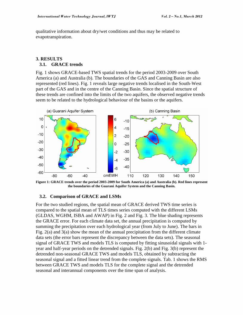
Fig. 1 shows GRACE-based TWS spatial trends for the period 2003-2009 over SouthAmerica (a) and Australia (b). The boundaries of the GAS and Canning Basin are alsorepresented (red lines). Fig. 1 reveals large negative trends localised in the South-Westpart of the GAS and in the centre of the Canning Basin. Since the spatial structure ofthese trends are confined into the limits of the two aquifers, the observed negative trendsseem to be related to the hydrological behaviour of the basins or the aquifers.

Figure 1: GRACE trends over the period 2003-2009 for South America (a) and Australia (b). Red lines representthe boundaries of the Guarani Aquifer System and the Canning Basin.

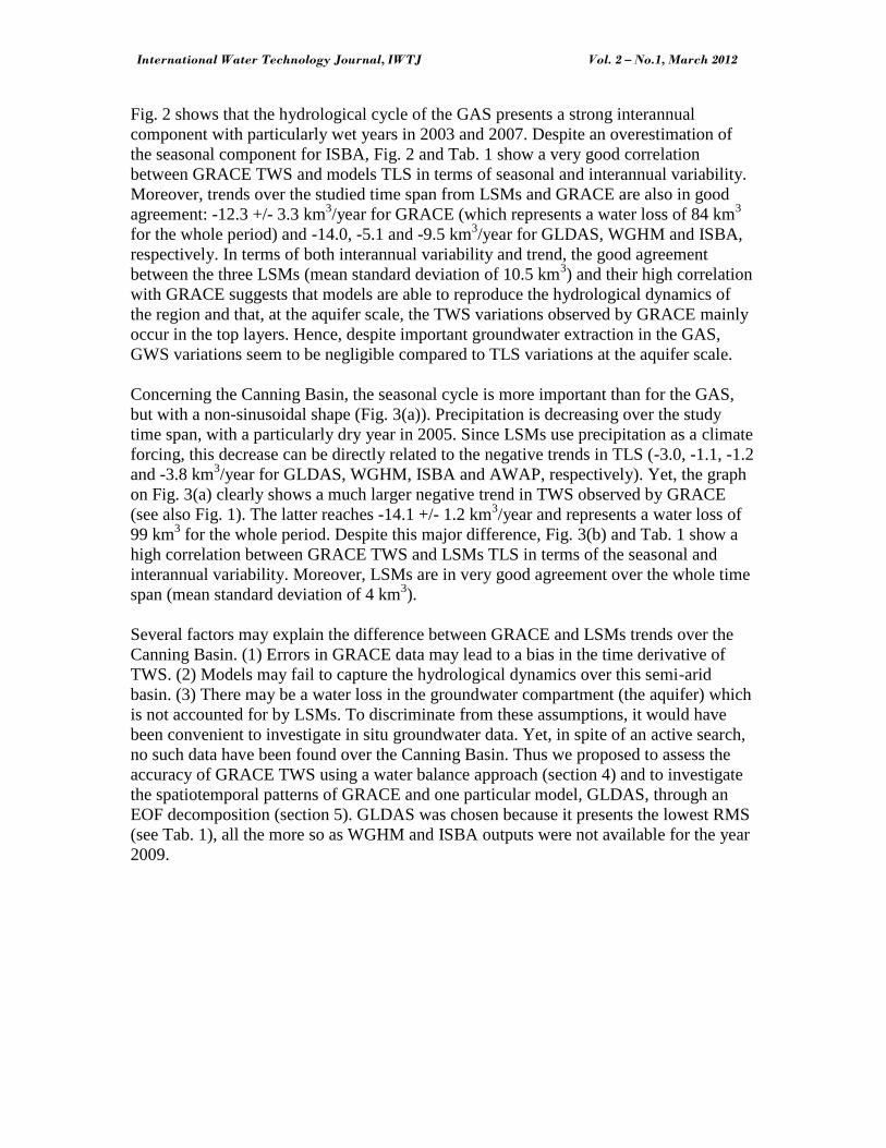
3.2. Comparison of GRACE and LSMs

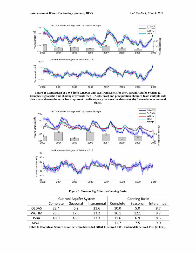
For the two studied regions, the spatial mean of GRACE derived TWS time series iscompared to the spatial mean of TLS times series computed with the different LSMs(GLDAS, WGHM, ISBA and AWAP) in Fig. 2 and Fig. 3. The blue shading representsthe GRACE error. For each climate data set, the annual precipitation is computed bysumming the precipitation over each hydrological year (from July to June). The bars inFig. 2(a) and 3(a) show the mean of the annual precipitation from the different climatedata sets (the error bars represent the discrepancy between the data sets). The seasonalsignal of GRACE TWS and models TLS is computed by fitting sinusoidal signals with 1-year and half-year periods on the detrended signals. Fig. 2(b) and Fig. 3(b) represent thedetrended non-seasonal GRACE TWS and models TLS, obtained by subtracting theseasonal signal and a fitted linear trend from the complete signals. Tab. 1 shows the RMSbetween GRACE TWS and models TLS for the complete signal and the detrendedseasonal and interannual components over the time span of analysis.


Fig. 2 shows that the hydrological cycle of the GAS presents a strong interannualcomponent with particularly wet years in 2003 and 2007. Despite an overestimation ofthe seasonal component for ISBA, Fig. 2 and Tab. 1 show a very good correlationbetween GRACE TWS and models TLS in terms of seasonal and interannual variability.Moreover, trends over the studied time span from LSMs and GRACE are also in goodagreement: -12.3 +/- 3.3 km3/year for GRACE (which represents a water loss of 84 km3

for the whole period) and -14.0, -5.1 and -9.5 km3/year for GLDAS, WGHM and ISBA,respectively. In terms of both interannual variability and trend, the good agreementbetween the three LSMs (mean standard deviation of 10.5 km3) and their high correlationwith GRACE suggests that models are able to reproduce the hydrological dynamics ofthe region and that, at the aquifer scale, the TWS variations observed by GRACE mainlyoccur in the top layers. Hence, despite important groundwater extraction in the GAS,GWS variations seem to be negligible compared to TLS variations at the aquifer scale.

Concerning the Canning Basin, the seasonal cycle is more important than for the GAS,but with a non-sinusoidal shape (Fig. 3(a)). Precipitation is decreasing over the studytime span, with a particularly dry year in 2005. Since LSMs use precipitation as a climateforcing, this decrease can be directly related to the negative trends in TLS (-3.0, -1.1, -1.2and -3.8 km3/year for GLDAS, WGHM, ISBA and AWAP, respectively). Yet, the graphon Fig. 3(a) clearly shows a much larger negative trend in TWS observed by GRACE(see also Fig. 1). The latter reaches -14.1 +/- 1.2 km3/year and represents a water loss of99 km3 for the whole period. Despite this major difference, Fig. 3(b) and Tab. 1 show ahigh correlation between GRACE TWS and LSMs TLS in terms of the seasonal andinterannual variability. Moreover, LSMs are in very good agreement over the whole timespan (mean standard deviation of 4 km3).

Several factors may explain the difference between GRACE and LSMs trends over theCanning Basin. (1) Errors in GRACE data may lead to a bias in the time derivative ofTWS. (2) Models may fail to capture the hydrological dynamics over this semi-aridbasin. (3) There may be a water loss in the groundwater compartment (the aquifer) whichis not accounted for by LSMs. To discriminate from these assumptions, it would havebeen convenient to investigate in situ groundwater data. Yet, in spite of an active search,no such data have been found over the Canning Basin. Thus we proposed to assess theaccuracy of GRACE TWS using a water balance approach (section 4) and to investigatethe spatiotemporal patterns of GRACE and one particular model, GLDAS, through anEOF decomposition (section 5). GLDAS was chosen because it presents the lowest RMS(see Tab. 1), all the more so as WGHM and ISBA outputs were not available for the year2009.


Figure 2: Comparison of TWS from GRACE and TLS from LSMs for the Guarani Aquifer System. (a)Complete signal (the blue shading represents the GRACE error) and precipitation obtained from multiple datasets is also shown (the error bars represent the discrepancy between the data sets). (b) Detrended non seasonal

signal.

Figure 3: Same as Fig. 2 for the Canning Basin.

Guarani Aquifer System Canning BasinComplete Seasonal Interannual Complete Seasonal Interannual

GLDAS 22.4 6.2 21.6 10.0 5.0 8.7WGHM 25.5 17.5 23.2 16.1 12.1 9.7

ISBA 48.0 46.3 27.3 11.6 6.9 8.5AWAP 11.7 7.5 9.0

Table 1: Root Mean Square Error between detrended GRACE derived TWS and models derived TLS (in km3).


4. VALIDATION OF THE GRACE-BASED TWS VARIATIONS OVER THE

CANNING BASIN

As done by Famiglietti et al. (2011), we validated the GRACE results by computing thewater budget given by Eq. (1) using essentially independent observations:

REPdt

d

TWS(1)

where P is the precipitation, E the evapotranspiration and R the runoff. Since the CanningBasin is located in a semi-arid region, the mean annual runoff may be neglected[http://www.anra.gov.au/topics/water/overview/wa/basin-sandy-desert.html] and thewater budget is essentially driven by P and E. We computed dTWS/dt for the GRGS andthe CSR GRACE solutions and P-E using the independent climate data sets presented insection 2.3. For the latter we computed independently the means of P and E beforecalculating the difference P-E. Besides, we associated an error from the dispersion ofindividual values around the mean. The mean uncertainty of P-E equals 3.0 km3/month.

Fig. 4 compares dTWS/dt with P-E. The blue and green shaded zones represent GRACEerrors, while the red shaded zone represents the uncertainties in P and E. First, thecomparison between the GRGS and the CSR solutions shows that both solutions agreewell within their respective error bars. The second graph also shows a good agreementbetween dTWS/dt and P-E. Namely, the temporal means over the common time period(2003-2007) are -1.7 and -2.0 km3/month for dTWS/dt and P-E, respectively (thus insidethe P-E uncertainty), which gives confidence in the TWS trend observed by GRACE overthe region. The good agreement between the different curves leads to the followingconclusions: (1) the GRACE data processing has a little effect on TWS in this region, and(2) GRACE well captures the hydrological dynamics over the basin.

Figure 4: Comparison of the time derivative of GRACE TWS from GRGS with the one from CSR (a) and withthe water budget estimate (b) for the Canning Basin. Blue and green shading represent the GRACE error while

red shading represents the water budget uncertainties.


5. SPATIAL AND TEMPORAL PATTERNS

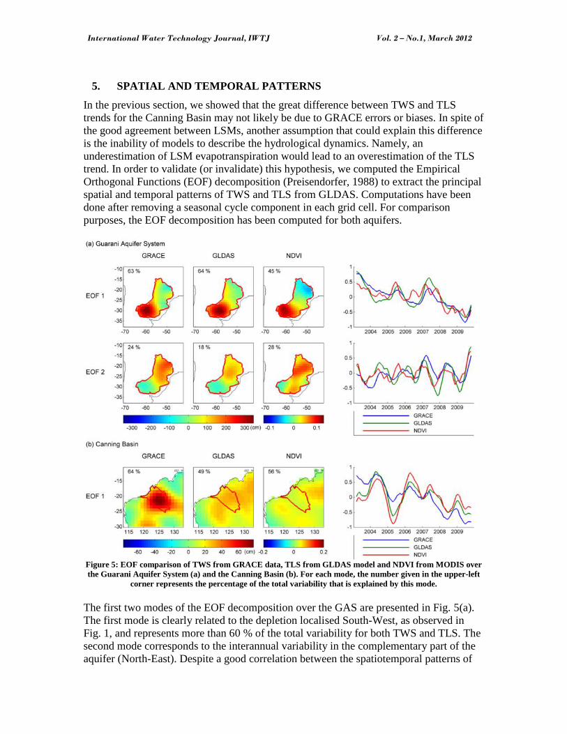
In the previous section, we showed that the great difference between TWS and TLStrends for the Canning Basin may not likely be due to GRACE errors or biases. In spite ofthe good agreement between LSMs, another assumption that could explain this differenceis the inability of models to describe the hydrological dynamics. Namely, anunderestimation of LSM evapotranspiration would lead to an overestimation of the TLStrend. In order to validate (or invalidate) this hypothesis, we computed the EmpiricalOrthogonal Functions (EOF) decomposition (Preisendorfer, 1988) to extract the principalspatial and temporal patterns of TWS and TLS from GLDAS. Computations have beendone after removing a seasonal cycle component in each grid cell. For comparisonpurposes, the EOF decomposition has been computed for both aquifers.

Figure 5: EOF comparison of TWS from GRACE data, TLS from GLDAS model and NDVI from MODIS overthe Guarani Aquifer System (a) and the Canning Basin (b). For each mode, the number given in the upper-left

corner represents the percentage of the total variability that is explained by this mode.

The first two modes of the EOF decomposition over the GAS are presented in Fig. 5(a).The first mode is clearly related to the depletion localised South-West, as observed inFig. 1, and represents more than 60 % of the total variability for both TWS and TLS. Thesecond mode corresponds to the interannual variability in the complementary part of theaquifer (North-East). Despite a good correlation between the spatiotemporal patterns of


GRACE TWS and GLDAS TLS for both modes, the graphs suggest a small difference inthe long-term trends of TWS and TLS: the GRACE trend seems to be lower (higher) thanthe GLDAS trend for the first (second) mode. Since the first (second) mode is related tothe southern (northern) part of the aquifer, we computed the TWS and TLS trends forthese two parts separately. In the northern part, TWS is increasing at a rate of 2.0km3/year whereas TLS is decreasing at a rate of 5.9 km3/year. In the southern part, TWSand TLS are decreasing at a rate of 36.2 and 27.9 km3/year, respectively. This resultssuggest that GWS is increasing in the northern part at a rate of 7.9 km3/year anddecreasing in the southern part at a rate of 8.3 km3/year. The groundwater depletion in thesouthern La Plata basin shown by Chen et al. (2010) with a similar methodology wasconfirmed by in situ data. Although these data concerned a region outside of the aquifer,their conclusion is in agreement with ours. Nevertheless, we showed in this study that thisdepletion is compensated, at the aquifer scale, by an increase in the northern part. Hence,at the aquifer scale, the main TWS variability corresponds to the top layers hydrologicalvariability.

Fig. 5(b) shows the first mode of the EOF decomposition over the region surrounding theCanning Basin. For GRACE TWS, a strong signal is centred over the basin (64 % of thesignal) and GLDAS TLS presents a quite similar but more diffuse spatial pattern (49 %of the signal). Both signals have a similar temporal evolution corresponding to negativetrends as shown in Fig. 3. The second mode presents a spatial pattern localised outsidethe basin, over the Kimberley Basin (North-East), and is therefore not presented here.

As written previously, NDVI informs on the "greenness" of Earth's landscapes. Highvalues represent lands covered by green, leafy vegetation and low values show lands withlittle or no vegetation. Since the vegetation development is directly related to theevapotranspiration, NDVI should be helpful to infer the ability of LSMs to well estimateevapotranspiration, especially during particularly dry of wet seasons when the vegetationdevelopment largely differs from normal conditions. Contrarily to Chen et al. (2010),who used this index for January 2009 as another proof of dry conditions in the lower LaPlata basin in early 2009, we used gridded time series of NDVI for a spatiotemporalpatterns comparison with GLDAS. To that purpose, we performed an EOFdecomposition of NDVI anomalies over the two regions. Corresponding leading modesare shown in Fig. 5.

The very good correlation between spatial and temporal patterns of the different signalsover the GAS (Fig. 5(a)) shows the relevance of the comparison with NDVI. Inparticular, NDVI very well captured the drought shown by GRACE and GLDAS in thesouthern part (likely responsible for a decrease in the vegetation development), as well asthe interannual hydrological variability of the northern part. For the Canning Basin (Fig.5(b)), NDVI presents a temporal pattern highly correlated to GLDAS TLS and to thedetrended GRACE TWS. Concerning the spatial pattern, NDVI is quite similar toGLDAS, with no strong signal centred over the basin. This suggests that the vegetationdevelopment decreased over the time span in the surrounding region (see the negativetrend on the temporal pattern), but not specifically over the Canning Basin, which is inagreement with the GLDAS analysis. Hence, the great negative trend of GRACE TWS


seems to be more likely due to a decreasing GWS at a rate of about 11 km3/year(difference between GRACE TWS and GLDAS TLS trends), representing a totalgroundwater loss of almost 80 km3 for the whole study period.

6. CONCLUSION AND DISCUSSION

In this paper, we used GRACE estimations of the Total Water Storage combined withLSM outputs to detect groundwater storage variations. The method was applied on twogreat aquifers with different climatic and anthropogenic characteristics, but both knownto have a high potential for domestic or irrigation use.

For the Guarani Aquifer System, no significant GWS variations were estimated at theaquifer scale, which means that (1) the main part of the hydrological dynamics (on a fewyears time scale) seems to occur mainly in the top layers and (2) groundwater extractionis currently negligible compared to the hydrological variability. However, the EOFdecomposition showed that a groundwater depletion at a rate of 8 km3/year may haveoccurred in the southern part of the aquifer and that this depletion have been compensatedat the aquifer scale by a GWS increase at the same rate in the northern part.

On the contrary, the important decrease in TWS (14 km3/year) observed in the CanningBasin seems to be mainly due to a groundwater depletion at a constant rate of 11km3/year (total water loss of almost 80 km3 for the whole study period). To assess this,the GRACE accuracy over the region has been inferred through a water balance approachand the model ability to well reproduce evapotranspiration has been validated by aspatiotemporal analysis and the comparison with NDVI. Since water use remains verylow in this sparsely populated region [http://www.water.gov.au], the observed depletionis certainly due to climate variability, i.e. sustained seasonal rainfall decrease over the lastfew years. This assertion is supported by Fig. 6 which shows the cumulative annualprecipitation in the Canning Basin over a longer time span (since 1950). First, the regionexperienced particularly wet seasons over the period 1995-2005, providing a large GWSsurplus. Then, the graph depicts a steady decrease in precipitation during the last decade,leading to a decrease in the aquifer recharge. This suggests that the decrease in GWScould be explained by a return to normal or even dry conditions. This result is inagreement with the interpretation given by van Dijk et al. (2011) who investigatedGRACE TWS retrievals over the whole Australian continent.

Figure 6: Long term annual precipitation over the Canning since 1950. The red curve shows the 7-years movingaverage and the green curve shows the temporal mean. The grey zone represents the period 2003-2009

considered in this study.


Despite different climate forcing and modelling schemes used by LSMs, the goodcorrelations between models for the two study cases provides a certain confidence in theirability to represent TLS. Consequently, this kind of study may be used to supportgroundwater management, especially in poorly monitored regions where no other data isavailable. As a perspective, GRACE gravity data may be used to improve hydrologicalmodels, namely by integrating relevant groundwater reservoirs (Ngo-Duc et al., 2007;Niu et al., 2007) or by assimilating GRACE data into models (Zaitchik et al., 2008).

ACKNOWLEDGEMENTS

We would like to acknowledge Markus Zaepke (BGR, Germany) for providing thecontours of both aquifers. We are grateful to Andreas Güntner (GFZ German ResearchCentre for Geosciences), Bertrand Decharme (CNRM, MeteoFrance) and Peter Briggs(CSIRO, Australia) for sharing WGHM, ISBA and AWAP outputs, respectively. We arevery grateful to Eric Wood (Princeton University, USA) for providing us withevapotranspiration data. We also thank Jean-Michel Lemoine (GRGS/CNES, France) forthe method to compute GRACE errors. M. Becker is financed by the ANR CECILEproject and S. Munier received a grant from the Centre National d'Etudes Spatiales(CNES, France).

REFERENCES

[1] Adler, R.F., Huffman, G.J., Chang, A., Ferraro, R., Xie, P.P., Janowiak, J., Rudolf, B.,Schneider, U., Curtis, S., Bolvin, D., Gruber, A., Susskind, J., Arkin, P., & Nelkin, E.,2003, The version-2 global precipitation climatology project (GPCP) monthlyprecipitation analysis (1979-present), Journal of Hydrometeorology, 4, 1147-1167, 2003.

[2] Alkama, R., Decharme, B., Douville, H., Becker, M., Cazenave, A., Sheffield, J.,Voldoire, A., Tyteca, S., & Le Moigne, P., Global Evaluation of the ISBA-TRIPContinental Hydrological System. Part I: Comparison to GRACE TerrestrialWaterStorage Estimates and In Situ River Discharges, Journal of Hydrometeorology, 11, 583-600, 2010.

[3] Becker, M., LLovel, W., Cazenave, A., Guntner A., & Cretaux, J.F., Recenthydrological behavior of the East African great lakes region inferred from GRACE,satellite altimetry and rainfall observations, Comptes Rendus Geoscience, 342, 223-233,2010.

[4] Becker, M., Meyssignac, B., Xavier, L., Cazenave, A., Alkama, R., & Decharme, B.,Past terrestrial water storage (19802008) in the Amazon Basin reconstructed fromGRACE and in situ river gauging data, Hydrology and Earth System Sciences, 15, 1607-7938, 2010.


[5] Bruinsma, S., Lemoine, J.M., Biancale, R., & Vales, N., CNES/GRGS 10-day gravityfield models (release 2) and their evaluation, Advances In Space Research, 45, 587-601,2010.

[6] Chen, J.L., Wilson, C.R., Tapley, B.D., Yang, Z.L., & Niu, G.Y., 2009 drought eventin the Amazon River basin as measured by GRACE and estimated by climate models,Journal of Geophysical Research, 114, B05404, 2005.

[7] Chen, J.L., Wilson, C.R., Tapley, B.D., Longuevergne L., Yang, Z.L., & Scanlon,B.R., Recent La Plata basin drought conditions observed by satellite gravimetry, Journalof Geophysical Research, 115, D22108, 2010.

[8] Decharme, B., Alkama, R., Douville, H., Becker, M., & Cazenave, A., GlobalEvaluation of the ISBA-TRIP Continental Hydrological System. Part II: Uncertainties inRiver Routing Simulation Related to Flow Velocity and Groundwater Storage, Journal ofHydrometeorology, 11, 601-617, 2010.

[9] Dirmeyer, P.A., Gao, X., Zhao, M., Guo, Z., Oki, T., & Hanasaki, N., GSWP-2:Multimodel Analysis and Implications for Our Perception of the Land Surface, Bulletinof the American Meteorological Society, 87, 1381-1397, 2006.

[10] Doll, P., Kaspar, F., & Lehner, B., A global hydrological model for deriving wateravailability indicators: model tuning and validation, Journal of Hydrology, 270, 105-134,2003.

[11] Famiglietti, J.S., Lo, M., Ho, S.L., Bethune, J., Anderson, K.J., Syed, T.H.,Swenson, S.C., de Linage, C.R., & Rodell, M., Satellites measure recent rates ofgroundwater depletion in California’s Central Valley, Geophysical Research Letters, 38,L03403, 2011.

[12] Foster, S., Hirata, R., Vidal, A., Schmidt, G., & Gardu˜no, H., The Guarani Aquiferinitiative: towards realistic groundwater management in a transboundary context,Technical report, Washington, D.C.: World Bank, 2009.

[13] Jin, Y., Randerson, J.T., & Goulden, M.L., Continental-scale net radiation andevapotranspiration estimated using MODIS satellite observations, Remote Sensing ofEnvironment, 115, 2302-2319, 2011.

[14] Leblanc, M.J., Tregoning, P., Ramillien, G., Tweed, S.O., & Fakes, A., Basinscale,integrated observations of the early 21st century multiyear drought in southeast Australia,Water Resources Research, 45, W04408, 2009.

[15] Longuevergne, L., Scanlon, B.R., & Wilson, C.R., GRACE Hydrological estimatesfor small basins: Evaluating processing approaches on the High Plains Aquifer, USA,Water Resources Research, 46, W11517, 2010.


[16] Ngo-Duc, T., Laval, K., Ramillien, G., Polcher, J., & Cazenave, A., Validation ofthe land water storage simulated by Organising Carbon and Hydrology in DynamicEcosystems (ORCHIDEE) with Gravity Recovery and Climate Experiment (GRACE)data, Water Resources Research, 43, W04427, 2007.

[17] Niu, G.Y., Yang, Z.L., Dickinson, R.E., Gulden, L.E., & Su, H., Development of asimple groundwater model for use in climate models and evaluation with GravityRecovery and Climate Experiment data, Journal of Geophysical Research, 112, D07103,2007.

[18] Preisendorfer, R.W., Principal Component Analysis in Meteorology andOceanography, New York, 1988.

[19] Raupach, M.R., Briggs, P.R., Haverd, V., King, E.A., Paget M., & Trudinger, C.M.,Australian Water Availability Project (AWAP): Final Report for Phase 3, CAWCRTechnical Report No. 013, Centre for Australian Weather and Climate Research (Bureauof Meteorology and CSIRO), Melbourne, Australia, 67 pp., 2009.

[20] Rodell, M., Houser, P.R., Jambor, U., Gottschalck, J., Mitchell, K., Meng, C.J.,Arsenault, K., Cosgrove, B., Radakovich, J., Bosilovich, M., Entin, J.K., Walker, J.P.,Lohmann, D., & Toll, D., The global land data assimilation system, Bulletin of theAmerican Meteorological Society, 85, 381-394, 2004.

[21] Rodell, M., Velicogna, I., & Famiglietti, J.S., Satellite-based estimates ofgroundwater depletion in India, Nature, 460, 999-U80, 2009.

[22] Rodell, M., Chen, J., Kato, H., Famiglietti, J., Nigro, J., & Wilson, C., Estimatinggroundwater storage changes in the Mississippi River basin (USA) using GRACE,Hydrogeology Journal, 15, 159-166, 2007.

[23] Schneider, U., Fuchs, T., Meyer-Christoffer, A., & Rudolf, B., Global PrecipitationAnalysis Products of the GPCC, Global Precipitation Climatology Centre (GPCC),DWD, Internet Publication, available online at: http://www.dwd.de, 112, 2008.

[24] Swenson, S.C., & Wahr, J., Post-processing removal of correlated errors in GRACEdata, Geophysical Research Letters, 33, L08402, 2006. Syed, T.H., Famiglietti, J.S.,Rodell, M., Chen, J., & Wilson, C.R., Analysis of terrestrial water storage changes fromGRACE and GLDAS, Water Resources Research, 44, W02433, 2008.

[25] Tapley, B.D., Bettadpur, S., Ries, J.C., Thompson, P.F., & Watkins, M.M., GRACEmeasurements of mass variability in the Earth system, Science, 305, 503-505, 2004.

[26] Tiwari, V.M., Wahr, J., & Swenson, S., Dwindling groundwater resources innorthern India, from satellite gravity observations, Geophysical Research Letters, 36,L18401, 2009.


[27] van Dijk, A.I.J.M., Renzullo, L.J. and Rodell, M., Use of Gravity Recovery andClimate Experiment terrestrial water storage retrievals to evaluate model estimates by theAustralian water resources assessment system, Water Resources Research, 47, W11524,2011.

[28] Wahr, J., Swenson, S., Zlotnicki, V., & Velicogna, I., Time-variable gravity fromGRACE: First results, Geophysical Research Letters, 31, L11501, 2004.

[29] Xie, P.P., & Arkin, P.A., Global precipitation: A 17-year monthly analysis based ongauge observations, satellite estimates, and numerical model outputs, Bulletin of theAmerican Meteorological Society, 78, 2539-2558, 1997.

[30] Zaitchik, B.F., Rodell, M., & Reichle, R.H., Assimilation of GRACE terrestrialwater storage data into a Land Surface Model: Results for the Mississippi River basin,Journal of Hydrometeorology, 9, 535-548, 2008.

Documents

USING GRACE TO DETECT GROUNDWATER STORAGE VARIATIONS: THE ... · using grace to detect groundwater storage variations: the cases of canning ... detect groundwater storage variations: