Using Gaussian Windows to Explore a

Multivariate Data Set

Louis A. Jaeckel

RIACS Technical Report 91.22

December 1991

https://ntrs.nasa.gov/search.jsp?R=19920019863 2020-05-12T14:31:50+00:00Z

Using Gaussian Windows to Explore aMultivariate Data Set

RIACS Technical Report 91.22December 1991

Louis A. Jaeckel

Work reported herein was supported in part by Cooperative Agreements

NCC 2-408 and NCC 2-387, between the National Aeronautics and Space

Administration (NASA) and the Universities Space Research Association (USRA).

Using Gaussian Windows to Explore a Multivariate Data Set

Louie A. Jaeckel

Research Institute for Advanced Computer ScienceNASA Ames Research Center

Moffett Field, CA 94035-1000

RIACS Technical Report 91.22December 1991

Abstract: This paper is a sequel to an earlier paper, in which I introduced themethod of "Gaussian windows" as a way of interactively exploring a set of quanti-tative multivariate data, in order to estimate the shape of the underlying densityfunction. In thispaper I recount an exploratory analysis, using Gaussian windows,of a data set derived from the Infrared Astronomical Satellite. My goals are todevelop strategies for finding structural features in a data set in a many-dimensionalspace, and to find ways to describe the shape of such a data set. After a brief reviewof Gaussian windows, I describe the current implementation of the method. I givesome ways of describing features that we might find in the data, such as clusters andsaddle points, and also extended structures such as a "bar", which is an essentiallyone-dimensional concentration of data points. I then define a distance function,which I use to determine which data points are "associated" with a feature. Datapoints not associated with any feature are called "outliers". I then explore the dataset, giving the strategies that I used and quantitative descriptions of the features thatI found, including clusters, bars, and a saddle point. I tried to use strategies and pro-cedures that could, in principle, be used in any number of dimensions

USING GAUSSIAN WINDOWS TO EXPLORE A A_ULTIVARIATEDATA SET

I. INTRODUCTION

This paper is a sequel to my earlier paper, "Gaussian windows:

A tool for exploring multivariate data" (Jaeckel, 1990). In that

paper I introduced the method of Gaussia, wi,do$s as a way of

interactively exploring a set of quantitative multivariate data, in

order to estimate the shape of the underlying density function.

The idea of the method is to examine the local structure of the

data in a given region by viewing the data through a Gaussian

window. If we assume that the density function in the window

region has a relatively simple form, we can find a local estimate

of the density function based on the eigenvalues and eigenvectors

of a matrix, as in the method of principal components. We can then

use our geometrical intuition to think about and describe the

features we find in the data. The method can be used to find and

describe structural features such as clusters (local maxima in the

density function), valleys, and saddle points, and also extended

structures such as a bar, which is an essentially one-dimensional

structure, or concentration of data points, consisting of data

points lying near a ce,ter li,e, but scattered about it in all

directions. By moving around in the space and taking many local

views of the data, we can form an idea of the structure of the data

2

set. The method is applicable in any number of dimensions. Since

the computations are relatively simple, the method can be

implemented on a small computer.

In this paper I will recount an exploratory analysis, using

Ganssian windows, of a data set derived from data gathered by the

Infrared Astronomical Satellite (I_AS). See IRAS Catalogs and

Atlases (1985) and Soifer et al. (1989). My purpose in performing

this analysis is twofold: first, to develop strategies for using

Ganssian windows to find local structural features in a real data

set; and second, to address the more general question of how to

comprehend and describe the shape of a data set in a many-

dimensional space, given that we have a method for estimating the

local shape of the data in any region. I will not attempt to do a

complete analysis of this data set.

I will begin in Section 2 with a very brief review of the

method. (A simi]ar brief review is given in Jaeckel, 1991.) Then,

in Section 3, I will describe the current implementation of the

method, which consists of a program written in BASIC. To explore a

set of data, the user can enter the parameters for a Ganssian

window, and the program will compute a variety of estimates based

on the data in the window region. This version of the program

restricts the user to spherical windows, rather than permitting

windows of any ellipsoidal shape. The program allows the user to

shift the window center along one or more of the eigenvectors just

found. This is useful for moving toward the center of an apparent

cluster or toward other features that may appear in a window. The

program can also do a cross-tab, that is, a kind of projection of

3

the data onto a two-dimensional subspace. It is often useful to

have a picture to look at, as long as we bear in mind that such a

projection may obscure important aspects of the structure of the

data.

In Section 4 I will give a way of describing features such as

clusters and bars, and a way to determine which data points are

associated with each feature. When a cluster, which appears as a

local maximum in the density function, is found, we can estimate

the density function (that is, the structure of the data) near the

ee,ter poi,t of the cluster. We can then compute the Mahala,obis

distaace of any data point from that center point. See Morrison

(1990). This is a distance function that is based on the shape of

the cluster. If the distance is small, then the data point can be

thought of as associated with the cluster. Note that since

features in the data may overlap, a data point may be associated

with more than one feature. In those cases I will not try to

decide which of those features a data point "really" belongs to; I

will just say that it could be part of any of them. If we find a

bar, that is, an essentially one-dimensional structure extending

for some distance through the space, we can describe it by choosing

a sequence of representative ce.ter poi,ts along the estimated

center line of the bar and by computing the estimated density

function near each of these center points. By using a somewhat

different definition of the Hahalanobis distance, we can measure

the distance of a data point from the estimated center line of the

bar, and we can then determine which data points are associated

with the bar. Those data points that are not associated with any

4

structural feature will be called outliers.

In Section 5 I will describe, in narrative form, my

exploration of the IRAS data set. I will discuss various

strategies for navigating in a many-dimensional space and

identifying features in the data, in the context of my analysis of

the data set. I worked with a random sample of 634 data points

drawn from the data set. There are four variables, or coordinates,

for each data point. After computing some standard overall

statistics, I looked at a cross-tab of the data (Figure 1), which

shows two apparent local maxima, or concentrations of data points.

For each cluster I found the estimated location of the center of

the cluster (the local maximum of the density function), the

estimated density at that point, an estimate of the proportion of

the data points that are part of the cluster, and the estimated

shape of the cluster.

It should be noted that all of the numerical estimates are

"soft" estimates, because they depend on the window size. Since

the clusters and other features we find do not have exact Ganssian

shapes, and since they often overlap, using windows with different

sizes gives different results. Choosing a window size means

choosing a scale, or level of resolution, at which to view the

data. This is because the quantities we compute are overall, or

summary, statistics for the data as seen through the window. Thus,

when we look at the data at different scales, we may see different

things. For example, in Figure 2, which shows the data on the

right side of Figure 1 from a different perspective, there seems to

be a narrow, dense cluster embedded in a broader cluster. Viewing

that part of the data with a large window shows the broad cluster,

while using a smaller window allows us to focus on the small inner

region where the data points have a much higher density. On the

other hand, if the estimated parameters of a feature are relatively

insensitive to small changes in the window size, I will consider

the feature to be "real". Since there is no absolute rule for

choosing a "best" window size, it is often helpful to experiment

with varying the window size to see how that affects the results.

Between the two main clusters visible in Figure 1 is a broad

region where the data points seem to have a lower density. If we

treat the complex cluster on the right as one peak, we can describe

the data in the central region as a bar running from one peak to

the other; that is, we can find a curved line about which the data

points are somewhat concentrated. We would expect to find

something like this when we have two overlapping clusters. If we

follow along the center line of this bar, we find a point where the

estimated density along the center line is minimized. This point

should be a saddle point in the estimated density function

(although for the data in Section 5 the saddle point and the point

of minimum density are slightly different). It is a useful element

of our description of the data set. I will describe the curved bar

by choosing a sequence of representative center points along the

estimated center line of the bar.

I said earlier that for each structural feature we find, such

as a cluster or a bar, we can determine which data points are

associated with that feature. After we have found a number of

features in the data, we can look for apparent outliers, that is,

data points that are not associated with any of the features found

so far. If there are groupings of points among these outliers,

they may indicate the presence of features we have not yet found.

If we then find more features, we can add them to our description

of the data set. After finding the features in the data mentioned

above, I searched through the data for outliers, and then I looked

at various cross-tabs of the outliers. I found a grouping of data

points that resembled a "finger" protruding from one of the

clusters, and another small group of points far off to one side. I

added these two features to the description of the data set, and I

repeated the search through the data for outliers. This time there

were no noticeable groupings among the outliers. About 5Z of the

data points were classified as outliers.

The final description of the data set consists of listing the

features found, with their descriptions. In this case I found some

clusters, a saddle point, and some bars. The clusters are each

described by the location of the center point, together with the

estimated parameters for that point. The saddle point is described

similarly. Each bar is described by a list of representative

center points, with the estimated parameters for each center point.

We could also list the outliers.

After I explored this random sample drawn from the data set, I

chose a second random sample in order to get an idea of the

variability of the estimates due to sampling error. The results

for the second sample are generally in agreement with the results

for the first sample.

Throughout my exploration of the data set, I tried to use

strategies and procedures that could be used in any number of

dimensions, at least in principle.

2. BRIEF REVIEW OF GAUSSIAN WINDOWS

Suppose that we are given a large set of quantitative

multivariate data, say, N data points xi in a p-dimensional

space, and that we want to explore the structure of the data. (For

the data set explored in Section 5, N = 634 and p = 4.) That

is, we want to find the shape of the underlying density function,

by looking for concentrations of data points. We will assume that

the density function is more or less smooth, but we will not make

any more specific assumptions about its structure. To explore the

data, we need a way to look at the local structure of the data in a

limited region. So we will examine the data in a given region by

viewing the data through a Gaussia_ wisdom, whose location and

shape are chosen by the user. We will describe the local structure

of the data by a method similar to the method of principal

components. We will then be able to find and describe simple

structural features in the data in any number of dimensions. By

taking many local views of the data, that is, by exploring the data

interactively, we can build up a description of the structure of

the data set.

Some examples of the kinds of structural features that we can

find and describe are the following: A peak, or relative maximum,

in the density function, which would appear as a cluster of data

points; a valley, or relative minimum; and a saddle point, where

the density function would be concave upward in some directions,

and downward in others. We can also find extended structures such

as a bar in the data, which is an essentially one-dimensional

structure, or concentration of data points, consisting of data

points lying near a ce,ter li,e but scattered about it in all

directions. Only a part of such an extended structure will be

visible in a single window. In a case like this we can tell that

we are looking at a structure that extends beyond the window, and

we can estimate the shape of the part of the structure that lies in

the window region. We can then follow along it and map out its

extent and shape. Similarly, we might find an essentially

k-dimensional structure in a p-dimensional space, for any k < p.

The approach here is different from that in the many graphical

methods that involve projecting the data onto a space of lower

dimension. See for example Chambers et al. (1983) and Cleveland

and McGill (1988). While these methods are often useful, such

projections may obscure some features in the data. However,

graphical methods can be used in conjunction with the method

described here, and I will often use cross-tabs, a kind of

two-dimensional projection of the data, to give me a picture of

part of the data.

I will use the notation used in Jaeckel (1990). That paper

gives complete derivations of the results outlined here.

To focus on a limited region in the space, we use a window. A

Gaussia. wi.dow is defined by choosing a center point a and a

nonnegative definite symmetric matrix V to describe its size and

shape. Let

t

- a)'V(x - a)w(x) = e _

where x is a p-vector and "prime" means "transpose". The matrix

V is analogous to the inverse of a covariance matrix. Each data

point x i is given the weight wi = w(xi). Note that w(a) = 1,

that w(x) _< 1 for all x, and that w(x) decreases as x moves

away from a. Thus we have defined a window with "fuzzy"

boundaries, rather than an ordinary window, for which each data

point would be either inside of the window or outside of it. The

function w(x) may be thought of as the relative transparency of

the window at x. That is, if each data point x i is a small

point of light with intensity 1, then, when viewed through the

window, it appears as a point of light with intensity wi. In

other words, the weight wi is somewhat like a "relative

probability" attached to the point. It can be shown that the shape

of the set of data points x i with weights wi attached resembles

the shape of the (improper) density function w(x)f(x), from which

it follows that if we do computations with the weighted xi, the

results will be somewhat as if we were working with an unweighted

random sample from w(x)f(x).

After choosing a window, we compute the weighted sample mean

vector,

= 1 Ewixi ,

and the weighted sample covaria.ee matriz,

Sw : 1-LEwi(xi - _w)(xi - _w)'Ewi

I0

We also compute _ Zwi. These quantities are the simplest things

to compute, especially in a high-dimensional space. They describe

the overall shape of the weighted data in the "window region" (the

region vaguely defined as the region where w(x) is "not small").

The estimated shape of the density function in the window region

will be based on these quantities. Note that these quantities are

overall statistics; any "fine structure" in the region is smeared

out. To look for finer details, we would use smaller windows.

Suppose first that in the region of a window, the density

function has approximately a multivariate Ganssian shape:

I -½(x- -

f(x) = c (2_)P/2]Zi1/2 e

where #, Z, and c are all unknown parameters. That is, we have

a single peak (or cluster of data points) in the window region.

The vector # is the center point of this part of the density.

The symmetric matrix Z is its covariance matrix. The constant c

represents the proportion of the entire data set that is contained

in the cluster; I will call this quantity the cluster mass.

Estimates of these parameters are derived in Jaeckel (1990), p. 29.

These estimates give us an estimate of the shape of the density

function in the window region.

If we find a cluster in a window, we can describe its shape

using the method of principal components. See Morrison (1990). To

do this we find the eigenvalues and corresponding eigenvectors of

Z, the estimate of Z. (I will use a _ above a parameter to

indicate its estimate.) The estimated shape of the cluster is a

11

p-dimensional ellipsoidal shape centered at _. The principal axes

of the ellipsoid are parallel to the eigenvectors. The estimated

density function can be expressed as a product of p univariate

Ganssian (normal) densities, each lying along a principal axis.

The standard deviation of each of these densities is the square

root of the corresponding eigenvalue (all of which are positive in

this case). Thus we have a way of thinking about the shape of the

cluster in any number of dimensions.

Note that we could do this analysis based on the matrix B,

defined below, which is the inverse of E. These two matrices have

the same eigenvectors, and the eigenvalues of B are the

reciprocals of those of _. It follows that a large positive

eigenvalue of B indicates that the data points are tightly

concentrated along the corresponding direction, while an eigenvalue

near 0 indicates a structure that may extend beyond the window

region. When we deal with more general structures, we will analyze

their shape by looking at the eigenvalues and eigenvectors of B.

The analysis above also applies if the shape of the density

function in the window region is like a valley or a saddle point.

In these cases all or some of the eigenvalues of B will be

negative. A negative eigenvalue indicates that, in the window

region, the density function is concave upward along the direction

of the corresponding eigenvector.

I will now give a more general formulation that will include

the examples above and also extended structures such as a bar.

Assume that in the window region the density function can be

approximated by

12

1f(x) = h e-_ x'Bx ÷ r'x ,

where h, r, and the symmetric matrix B are unknown parameters.

The exponent is a general polynomial of degree two in the

coordinates of the vector x. (Any constant term is absorbed in

h.) I will assume for simplicity that ,, the window center, is

0. The constant h = f(O) is the density at the window center.

The symmetric matrix B may or may not be positive definite, and

it may or may not be nonsingular. If B is positive definite,

then f(x) describes a cluster with a multivariate Gaussian shape,

for which B is the inverse of the covariance matrix. In this

case f(x) can be expressed in the form given earlier. For other

features, such as a saddle point or a bar, B might have some

eigenvalues that are negative or zero.

We compute _w' Sw, and _£w i, and we estimate the

parameters B, r, and h based on these quantities. The

estimates are derived in Jaeckel (1990), p. 36. Let A = B + V.

It turns out that Sw, the weighted sample covariance matrix, is an

estimate of A-1 so we can estimate A

-1 = _ = _ ÷ V. So we can estimate BSw

= Sw-1 - V .

by

by

Sw-1, and we have

We then find the eigenvalues and eigenvectors of B, and we use

these quantities to describe the shape of the estimated density

function in the window region. The method is analogous to the

method of principal components, except that B plays the role of

the inverse of a covariance matrix. The interpretation of the

13

eigenvalues of B is as stated above. As in principal components

analysis, we can express the estimated density function as a

product of p functions of one variable each.

Let _1' _2' "" ' _p be the eigenvalues of B, and let z 1,

z2, ... , Zp be a set of eigenvectors corresponding to the _j,

chosen so that they are mutually orthogonal and each of unit

length. (The zj are not uniquely determined by these conditions,

but that does not matter.) Let Z be the orthogonal matrix whose

columns are the zj. We will now make a change of coordinates so

that the zj form an orthonormal basis for the new coordinate

system. A vector x in the original coordinate system is

represented by y = Z'x in the new coordinate system; that is, the

jth coordinate of the point x in the new coordinate system is

yj = zj'x. In this coordinate system B becomes

matrix. If we let tj = zj'Sw -1 _w' then we can writediagonala

the estimated density function as

_I x'Bx + f'x _ 1f(x) = h e _ = h e-_ _jyj2 + tjyj ,

where the yj are the variables in the new coordinate system. See

Jaeckel (1990), pp. 37-38. Note that the computations involved are

simple matrix operations.

The estimated density function is now a product of p

functions of one variable each, where each of these functions is

14

either an ordinary univariate Gaussian function if _j > O, or a

"concave Ganssian" function if ]j < O. If _j = O, the function

is an exponential function or a constant. If _j > O, then 2j-1

is the variance of the Ganssian shape, and _j-1/2 is its standard

deviation. If _j < O, we can interpret (_]j)-l/2 as a scale

parameter analogous to the standard deviation. In each case, _j

is related to the curvature of the function.

For any j for which _j _ O, we can complete the square for

the expression in the exponent for that j:

"7 _jyj2 + tjyj = -7 Yj - +

If we let yj = _., that is, if we move along the axis vector zjJ

t.

for a distance of _, we come to the "center" of the function ofJ

yj along that direction. At this point we have either a maximum

or a minimum of the jth function in the product above, depending

t.

on the sign of Aj. It follows that the point _j zj is the

nearest point to the origin for which that function is maximized or

minimized. If Aj is near O, then instead of completing the

square along the direction of zj, we may want to assume that we

have, approximately, an exponential function or a constant in that

direction. Geometrically, this amounts to concluding that, along

this direction, we are looking at part of a large structure, such

as a ridge or a gradual slope, that extends beyond the window

region. If none of the Aj is 0, so that _-I exists and _, the

center of the estimated density function, is defined, then the

15

t°

point _j zj is the projection of _ on the line generated by

zj. Also, note that tj is the first partial (or directional)

derivative of log f(x) with respect to yj at the window center.

We can now handle the case of an extended structural feature,

such as a bar of data points, that passes through a window and

extends beyond it. In this case B will have some eigenvalues

very near O. Since B is like an estimated inverse covariance

matrix, an eigenvalue near 0 indicates that the data in the window

region appear to have an essentially "infinite" variance in the

direction of the corresponding eigenvector. In the case of a bar,

which is an essentially one-dimensional concentration of data

points, B will have one eigenvalue very near O, and the

corresponding eigenvector will be parallel to the estimated center

line of the bar. Since a structure like this does not have a

center point, as a cluster does, we will not try to estimate a

center point here. Instead, we will estimate the location of the

center line of the bar, as in Jaeckel (1990), pp. 51-52. We can

also use the p - 1 remaining eigenvalues and eigenvectors to

estimate the shape of the (p-1)-dimensional cross section of the

bar orthogonal to the center line. If we find a bar in the data,

we can then move the window center to the nearest point on the

estimated center line and try another window. Then we can follow

along the bar by moving the window center along the estimated

center line. By continuing in this way we can map out the extent

and shape of the bar. An essentially k-dimensional structure, or

concentration of data points, can be treated in a similar way.

16

Since the method is interactive, it is flexible and

open-ended. It can be used (in principle) in any number of

dimensions. Few assumptions are made about the data. We can

search for structural features by trying many different windows,

and we can describe the features we find. Then we can put together

what we have found into an overall description of the data. The

method can be used in conjunction with other methods, such as

graphical methods and automatic clustering algorithms. Note that

with this method ue can find structural features other than

clusters. Since the computations are relatively simple, the method

can easily be implemented on a small computer. Any standard

algorithms for inverting a matrix and for finding the eigenvalues

and eigenvectors of a symmetric matrix can be used. Most

importantly, we can apply our geometrical intuition to the features

we find in the data, so that we can think about and describe the

structure of a set of data in any number of dimensions.

3. IMPLEMENTATION OF GAUSSIAN WINDOWS

_y current implementation of the method is a program vritten

in BASIC that runs on an IBM PS/2 with the DOS 3.3 operating

system. This implementation permits only spherical windows, rather

than windows of any ellipsoidal shape. This restriction allows the

computations to be somewhat simpler than in the general case.

To define a window, the user chooses a p-vector a to be the

window center, and a positive number to be the windo¢ sta,dard

deviatio,, or WSD. The matrix V defining the shape of the

17

spherical window is

where v = 1/(WSD) 2

V=vI ,

Thus V is a multiple of the identity

matrix, and the window is spherical because w(x) is a function of

the Euclidean distance between a and x. If we think of V-1 as

the "covariance matrix" of the window, then every vector is an

eigenvector and the WSD is the common standard deviation along

every direction. Since the WSD acts as a scale factor, it is easy

for the user to think about the size of the window in terms of this

parameter. (If we want V = O, that is, a window with "infinite"

standard deviation, in which case w(x) = 1 for all x, then we

enter 0 for the WSD.)

The program then makes one pass through the data set and

computes the summary statistics _w' Sw, and Ewi, based on the

weights assigned to the data points. In the general case, where

the window could have any ellipsoidal shape, the next step would be

to invert Sw. However, if the data points in the window region

lie in or near a linear manifold, then Sw will be singular or

nearly singular, and attempting to invert it could cause numerical

problems. For this reason I assumed in Jaeckel (1990), p. 25, that

the data points do not lie in a linear manifold. It can be shown

that if we use only spherical windows, we do not have to invert Sw

m although my program does it anyway D and we will not have to

make the above assumption. The quantities that we want to estimate

can be computed from the eigenvalues and eigenvectors of Sw,

although some of them will be undefined if Sw cannot be inverted.

The next step in the general case would be to compute the

18

= Sw-I - V, the estimate of the matrix B that definesmatrix

the shape of f(x) in the window region. Ne would then find the

But if V =

Sw-I

Ul, "" ,

are the

eigenvalues _j and a set of eigenvectors zj of B.

vI, we can do the following: Note first that Sw and

(assuming it exists) have the same eigenvectors, and if

Up are the eigenvalues of Sw, then Ul-I, ... , Up-I

eigenvalues of Sw-I. Also, uj _ 0. I will now show that

Sw-I - vI has the same eigenvectors as Sw and Sw-1. If

an eigenvector of Sw, then

Bzj : Sw-lzj - vIzj : uj-lzj - vzj = (uj-I - v)zj

zj

Thus zj is an eigenvector of

is

and the corresponding eigenvalue

So, instead of working with B, the program finds a set of

eigenvectors and eigenvalues for Sw, and then, for each positive

uj, it uses the formula above to compute _j. (If uj is very

close to 0, then _j is considered to be "infinite". This would

occur if the data lie very near a linear manifold.)

Some of the computations involve _j-1 It can happen that

is 0 or very close to 0, in which case _j-1 would be infiniteAj

or very large. This would occur if, in the window region, the

shape of f(x) along the direction of the corresponding

eigenvector zj is nearly constant or exponential. Such a shape

would appear to extend beyond the window region along zj. In this

the program sets Aj-I to some arbitrary very large number;case

is

1 - u.v

_j = uj-I - v = ujJ

19

its exact value does not matter. By working with Sw instead of

B, the program avoids some numerical problems that might occur when

_j is near 0 or near infinity.

The program has a number of features for handling the data,

displaying the results of using a window, moving the window center

to a new point, saving certain information, and displaying two-

dimensional projections of the data. After doing the computations

for a window, the program displays the eigenvalues and eigenvectors

and the estimated density at the window center. If all of the ]j

are positive, in which case we have an apparent cluster, the

program computes the estimated cluster mass, defined in Section 2.

The program also displays the standard deviation along each

principal axis (or the analogous quantity for a negative _j), thet.

first partial derivatives t j, the distance 1_. along each axis toJ

the maximum or minimum in that direction, and the same distance in

"standard units" (the distance divided by the standard deviation).

To shift the window center to a new location based on the

results of the current window, the program allows the user to move

the window center any desired distance along any of the

eigenvectors. This is useful for climbing toward a local maximum

or toward the center line of a bar, and also for moving along the

estimated center line of a bar. See Jaeckel (1990), pp. 50-53.

The program can display a cross-tab of the data, constructed

as follows: The user enters two vectors, or the program uses the

first two eigenvectors found for the current window. The data

points will be projected onto the plane generated by those vectors.

20

The user also enters a minimum and a maximum value for each

coordinate in that plane. These values define a rectangle in the

plane, which is divided into a 16-by-16 array of "bins" of equal

size. The program counts the number of data points whose

projection falls into each bin and displays the results, as in

Figures I and 2. (The rest of the plane is divided into semi-

infinite rectangles by extending the lines defining the bins; the

program also displays the numbers of data points in those regions,

although they are not shown in the two figures.)

The program can also perform the operations discussed in the

next section.

4. DESCRIBING _TIATl_EFIND IN ThE DATA

Perhaps the most fundamental issue in exploring a data set is

how to describe what we find in the data, so that we can develop an

understanding of the structure of the data set. In this section I

will give a simple way to describe clusters and bars. I will then

define a distance function which I will use to determine which data

points are associated with a feature. Those data points that are

not associated with any features will be called o,tliers.

Suppose that we find a peak, or local maximum, in the

estimated density function, that is, the center of an apparent

cluster of data points. When I find an apparent peak in a window

region, I try another window centered at that point, and I repeat

this process a few times until the window center converges to the

local maximum. If we try a Gaussian window centered at the local

21

maximum, with a WSD chosen so that a large part of the cluster

appears in the window region, and if no other significant features

appear in the window region, then all of the Aj will be positive,

the first partial derivatives tj will be very near O, and the

standard deviations along the eigenvectors will all be less than

about one or two times the WSD. I will call this local maximum a

ce,ter poi,t, since it is the apparent center of a cluster. (The

program can save the following information about each center point

for later use: its location, the eigenvectors and eigenvalues of

B, and the WSD of the window used to find this information.) There

are some other numbers that we can include in a quantitative

description of the cluster. First, we can estimate the density --

the value of f(x) --at the peak. This estimate is useful for

purposes of comparison. We can also ask how much of the data is

contained in the cluster. We must be careful with our terms here,

since a cluster may have some overlap with other clusters or with

other features. One quantity we can estimate is the cluster mass,

based on the assumption that the cluster has a multivariate

Gaussian shape. This was defined in Section 2 as the proportion of

the data that is contained in the cluster. I have found that the

estimated cluster mass must be used with care, since if any of the

standard deviations is large, which would mean that a substantial

part of the apparent cluster is outside of the window region, then

the estimate may be very unstable numerically, and not very

meaningful anyway. As a general rule, the estimated quantities are

meaningful (and numerically stable if they are based on a

reasonable amount of data) only if they refer to some geometrical

22

property of the data in the window region.

We can also ask which of the data points belong to a cluster

in some sense. I will say that a data point is associated with a

cluster if it is near the center point in the sense defined below.

Note that by this definition a data point may be associated with

more than one cluster or other feature. For example, we might find

two local maxima not very far apart from each other, which would

suggest that we have two overlapping clusters, in which case some

of the data points would be associated with both clusters. I will

not try to draw a boundary between two such clusters, or to

determine a quantitative "relative likelihood" that a point belongs

to one cluster or to the other. Any such computations would be

dependent on making rather specific assumptions about the shapes of

the clusters, which I do not want to make. Instead, I will just

let the description of features like this be "two overlapping

clusters", or "a shape like a dumbbell", and I will consider some

data points to be associated with both clusters.

t/hen we find two peaks, it may be useful to search for a bar

leading from one peak to the other (like a ridge joining two

hills), and to look for a saddle point along the bar, which would

represent a point of minimum density along the center line of the

bar. Comparing this minimum density along the bar with the

densities at the peaks will give us an idea of the nature of the

overlap, or connection, between the two clusters. We will see an

example of this later.

I will now define a measure of distance in terms of the shape

of a cluster. Suppose we have found a cluster with estimated

23

center _ and estimated inverse covariance matrix B. Then, for

any point x, let

D2 = (x - _)'B(x - _)

The quantity D is known as the iahalaBobis distance between x

and _. See Horrison (1990). I will call it the I-distasce. It

is sometimes used for classifying points as belonging to one of

several populations. Since the estimated density function for the

cluster is a function of D2, the set of points for which D2 is a

given constant is an ellipsoidal shell about _, on which the

estimated density is a constant. We can transform the expression

above by using the coordinate system with origin at _ and with

basis vectors the eigenvectors zj of B. Then, in that

coordinate system, x - _ becomes y = Z'(x - _) and B becomes

L = Z'B Z, where L is the diagonal matrix defined in Section 2,

whose entries along the main diagonal are the _j. Then

P

D2 = (x - _)'B(x - _) = y'Z'B Zy = y'Ly = _ ]jyj2

j=l

If we assume that a cluster has a multivariate Ganssian shape,

then the proportion of the cluster that lies within one of these

ellipsoidal shells may be found from the chi-square distribution

with p degrees of freedom. For example, if p = 4, then 95Z of

the mass of the cluster will lie in the region defined by D_ <

9.488, which is the upper 5Z point of the chi-square distribution

with 4 degrees of freedom. That is, a point chosen at random from

a Gaussian cluster would have a 95Z chance of lying in this region.

Using this value as a cutoff value, I will say that a data point

24

xi is associated at She 957, level with the cluster if D2 < 9.488

for that x i. We can then compute D_ for each data point to see

which ones are associated with the cluster, by this definition.

Approximately 95Z of the data points that "should be" considered

part of the cluster will pass this test. Thus, for a Ganssian

cluster, the proportion of the data points that are associated with

the cluster should be roughly 95_ of the estimated cluster mass.

Suppose that we find a bar, that is, an essentially one-

dimensional structure, in a _indo_ region. We can move the _indo_

center to a point on the center line of the bar, and then move

along the bar, to trace out its extent and shape. See Jaeckel

(1990), pp. 50-53. A simple way to describe a bar is to choose a

sequence of representative ee_ler poinSs _k along the estimated

center line of the bar, and, for each such point, to record its

location, the estimated density there, the eigenvectors and

eigenvalues describing the shape of the bar, and also the WSD of

the window used to find these estimates. (The window used for

computing these estimates would be centered at the center point.)

The WSD gives us some idea of the region in which these estimates

might be valid. The chosen center points should be close enough to

one another so that the window regions overlap. We can then be

confident that we are following a continuous bar, and that we have

reasonable estimates of its shape all along it.

In some cases it may be desirable to fit a curve of some sort

to this sequence of center points, so that we have a smoother

description of the bar, but I will not do that here. To keep the

description simple, I will just describe the bar by listing the

25

sequence of center points with their estimated parameters. By

looking at this sequence, we can get a sense of where the bar is

and how it is shaped.

We will now define the distance from a data point to the

estimated center line of a bar, by a method similar to the one we

used above for clusters. Let x be a point in the space. I want

to define a distance, analogous to the M-distance defined above,

from x to the estimated center line, rather than from x to any

one of the chosen center points. Let _k be one of the

representative center points we have chosen along the estimated

center line. Since we have a bar, one of the eigenvalues computed

at _k' say _p, will be near O. Let Zp be the corresponding

eigenvector. The estimated center line, at least in the region

near _k' is the line through _k generated by Zp. If we project

x onto this line, we will find a point x*, which is the point on

the line closest to x. The line segment from x to x* is

orthogonal to Zp; that is, the segment lies within a slice through

the bar orthogonal to Zp. We can therefore define a length for it

based on the estimated shape of the (p-1)-dimensional cross section

of the bar. Expressed in the coordinate system generated by the

zj, the (p-l)-dime,sio,al I-dista,ce from x to x*, the nearest

point on the estimated center line, is the square root of:

p-1

D2 = _ Ajyj2

j=l

In other words, we took the (p-1)-dimensional slice through the bar

containing x and we found the M-distance, within that cross

26

section, from x to x*, the point on the center line.

Note that for a given x this computation can be carried out

for any of the center points _k" But we should not use this

distance formula if x* is far from _k' because the bar might

curve or change its shape or even disappear as we move along it.

That is, the estimates of the center line and the shape of the

cross section at each _k are local estimates, and they may not be

valid outside of the region of the window on which they are based.

As a rule of thumb, I consider the (p-1)-dimensional M-distance to

the estimated center line to be meaningful only if the (Euclidean)

distance between x* and _k is less than the WSD of the window

used to find the estimates at _k"

_e can now determine which data points are associated with the

bar. If we choose a cutoff value for D2, say the upper 57 point

of the chi-square distribution with p - 1 degrees of freedom, we

can then say that a data point x i is associated at the 957. level

with the bar if, for at least one of the _k:

1) the (p-1)-dimensional M-distance from x i to the

estimated center line is less than the cutoff value; and

2) the corresponding x* is within one WSD of that _k"

For example, if p = 4, then the criterion for the three-

dimensional M-distance would be D_ < 7.815. Roughly 95_ of the

data points that "should be" considered part of the bar will pass

this test. Note that a data point may satisfy this twofold test

for more than one of the _k" The region that would contain data

points associated with the part of the bar represented by a

particular _k is shaped like a segment of a cylinder, whose cross

27

section is a (p-1)-dimensional ellipsoid. If the chosen center

points _k are not too far apart, these cylindrical segments will

have enough overlap so that even if the center line is curving,

most of the bar will be included in one or more of the segments.

(These segments might also overlap with other features.) This

union of cylindrical segments is somewhat crude, but it gives us a

general description of the part of the space that is occupied by

the bar.

_y reason for using cutoff values based on the chi-square

distribution is this: Granted that the cutoff values for D2 are

arbitrary, I wanted to use values that had equivalent meanings in

different numbers of dimensions. If we use the upper 5Z point with

p degrees of freedom for clusters and the corresponding point with

p - 1 degrees of freedom for cross sections of bars, and if these

features are truly Gaussian in shape, then in each case about 95Z

of the data points that are part of these features will be

classified as associated with the features.

After we have found some structural features in the data, we

can look for outliers, that is, data points that are not associated

with any of the features found so far. Some of these apparent

outliers may belong to features that we have not yet found, and

some of them may be true outliers, belonging to no identifiable

feature or concentration of data points. By examining some of

these outliers, either with Ganssian windows or simply by looking

for groupings of points in cross-tabs or other pictures of the

outliers, we may be able to locate new features in the data and add

them to our description of the data set. A grouping of outliers

28

might turn out to be an appendage of a previously found feature;

for example, we might find a bump protruding from the side of a

cluster, or the shape of a cluster might deviate from an ellipsoid

in some other way. Such features can be accounted for in our

description of the data set by adding one or more center points to

our list, together with the relevant parameters. Since I am freely

allowing features to overlap, without trying to decide which

feature each data point belongs to, we can include as many items in

our description as we think are needed to cover most of the data

points. Ne can continue this process until the remaining outliers

no longer appear to contain any features.

5. EXPLORING THE IRAS DATA SET

In order to experiment with Gaussian windows on a real data

set, I obtained a set of astronomical data from Peter Cheeseman of

the Research Institute for Advanced Computer Science at the NASA

Ames Research Center. The Infrared Astronomical Satellite (IRAS),

launched by NASA in 1983, found several thousand objects that emit

infrared radiation at various wavelengths.

Atlases (1985) and Soifer et al. (1989).

the data using a program called AUTOCLASS.

(1988).

See IRAS Catalogs and

Cheeseman has analyzed

See Cheeseman et al.

The data set that I will explore, and that I will refer to as

the "IRAS data set", was derived from da_a gathered by the

satellite. It consists of measurements on 6338 point-source

infrared emitters. For each source there are four variables

29

representing radiation intensity at various infrared wavelengths,

together with the galactic longitude and latitude of the source,

and various other information. The four infrared variables are

described as:

1. Flux magnitude for 12 microns

2. Difference of 12 and 25 micron flux magnitudes

3. Difference of 25 and 60 micron flux magnitudes

4. Difference of 60 and 100 micron flux magnitudes.

(I have been told that these "differences" are actually ratios, but

for my purposes it does not matter; I assume that the data have

been transformed in a way that is meaningful to astronomers.) In

my analysis I used only these four variables, without considering

the other information about the sources.

I should emphasize that I am not attempting to give a

definitive analysis of this data set. Instead, I am using the data

set to gain experience in using Gaussian windows, to experiment

with various strategies for exploring large data sets, and to try

out various enhancements to my computer program. Rather than

trying to give any substantive interpretations to the features that

I find in the data, I will treat the data as a set of points that

may have some internal structure, and my main goal will be to try

to discover and describe some of that structure. In a more

real-life situation the researcher would be guided in part by his

or her substantive knowledge about the data, including any

assumptions, hypotheses, or guesses about how the variables might

be related, and by whatever the researcher considered to be

significant.

3O

Since my program in written in BASIC and it runs on a small

computer, it runs relatively slowly and has limited memory

capacity. So I decided to work with a subset of the entire data

set. I chose a systematic random sample by selecting every tenth

data point, beginning with the third. The number of data points in

my sample is N = 634. Since I am using only the four variables

above, p = 4.

I began by computing some simple statistics to get an overall

picture of the data set. I computed the means, standard

deviations, minimum values, and maximum values for each of the four

variables. The results are as follows:

Variable Mean Standard Dev. Minimum Maximum

1 2.31 2.12 -5.65 5.51

2 2.00 1.13 -.03 6.29

3 3.07 1.83 -.78 6.25

4 1.88 1.03 -.59 4.36

At this point I considered whether to "normalize" the data,

that is, separately for each variable, to subtract the mean and

divide by the standard deviation. Since the standard deviations of

the variables are not that different from each other, I decided not

to normalize the data, but to work with the numbers as they are.

It should be noted that the results of the Gaussian windows

computations, which are based on the eigenvalues and eigenvectors

of B, are not invariant under scale changes applied to the

variables, just as the method of principal components is not

invariant under such scale changes. See Norrison (1990).

31

I then did a principal components analysis; that is, I ran the

Ganssian windows program using a window of "infinite" radius

(v = 0), so that the data points were given equal weight. (Any

point can be used as the window center in this case.) The

eigenvector corresponding to the largest eigenvalue of the sample

covariance matrix, normalized to have unit length, is z 1 =

(.73, .19, .60, .26). The line through the sample mean generated

by z 1 is the longest principal axis of the cloud of data points.

If we project the data points onto this line, the resulting set of

points on the line comprises the first principal component of the

data. The standard deviation of these values is 2.70, the square

root of the largest eigenvalue of the sample covariance matrix.

The first principal component accounts for 71Z of the total

variance in the data.

To obtain a first graphical view of the data, I did a

cross-tab that consisted of projecting the data onto the two-

dimensional subspace generated by z 1 and z2, the eigenvectors

corresponding to the two largest eigenvalues of the sample

covariance matrix. A part of the plane is divided into squares, as

described in Section 3, and the number of data points falling in

each square is tabulated. The result is shown in Figure 1.

(Projecting onto this plane preserves more of the total variance

than projecting onto any other plane. This does not mean, of

course, that this projection is the most informative one to use.

But it is a place to start.) As can be seen from the picture, the

data points do not form an ellipsoidal cloud, as is sometimes

tacitly assumed when doing principal components analyses. There

32

seem to be two distinct peaks, with a large area around and between

the peaks where many data points are spread out at a lower density.

There could be other features in the data that are obscured by this

two-dimensional projection. _e will use Gaussian windows to

explore the features in the data in more detail, and to describe

them quantitatively.

8ne of the quantities we will estimate is the value of the

density function at various key points. To obtain a benchmark

value for purposes of comparison, imagine that the cloud of data

points has a multivariate Gaussian density function whose

parameters are given by the overall sample mean and sample

covariance matrix computed above. If we use that density function

to give us an estimate of the density at the sample mean, the point

at which that density function is maximized, we obtain an estimate

of .013. Since we clearly do not have an ellipsoidal shape, this

value is not a meaningf,1 estimate of the density at the sample

mean. In fact, we will see that there are points at which the

estimated density is much greater than .013. Thus we could not

adequately describe the data set by any method that was based

solely on the overall sample mean and sample covariance matrix.

THE CLUSTERON THE RIGHT

Now we will begin using Gaussian windows.

I decided first to locate the apparent peak, or local maximum,

in the density toward the right side of Figure 1. Based on the

cross-tab and the information on the principal components, I began

at the sample mean and I moved from there along the first

33

eigenvector a distance of 2 in the positive direction. I tried a

Gaussian windowusing that point as the window center, and a WSDof

2, so that a large amount of the data in the right side of the

cross-tab would be in the window region. A local maximumappeared

in the window region; that is, all four _j were positive and the

distance along each eigenvector to the apparent maximum in that

direction was not large, compared to the WSD. This local maximum

is of course not our final estimate; it is just the first step. I

then moved toward the peak in several steps, as described below,

until I had a window for which the estimated peak was at the window

center. I usually proceed conservatively, making relatively small

changes in the window center and/or size at each step. (This is

why it is desirable to have a procedure for which the computations

are simple.) Since it seemed that with WSD = 2, too much weight

is given to data points that are not part of the cluster, I

gradually reduced the window size. After trying the first window I

moved the window center to the apparent local maximum as seen in

that window and I reduced the WSD to 1.5, still a fairly broad

window. A new peak appeared in this window, not far from the

previous one. I then moved the window center to that point and

kept the WSD at 1.5. After another one or two windows with WSD =

1.5 and small changes in the window center to bring it to the

local maximum, I determined that there is a local maximum at

(3.61, 2.21, 4.25, 2.30). (These estimated coordinates are

actually "soft" numbers, because they depend on the choice of the

WSD. I will return to this issue below.) At that point the first

partial derivatives tj are all essentially zero, all of the Aj

34

are positive, and none of the standard deviations along the

eigenvectors is large compared to the WSD.

The eigenvectors and the corresponding standard deviations,

which describe the shape of the cluster around this point, are:

Eigenvector Standard Deviat ion

( .80, -.49, .04, .35) 1.32

(-.50, -.48, .59, .41) 1.02

( .34, .46, .80, -.21) .88

( .00, .57, -.11, .82) .42

The estimated density at this peak is .036, almost three times the

fictitious density estimate we found earlier for the sample mean.

The estimated cluster mass for the cluster about this peak is .72;

that is, about 72% of the data should belong to this cluster. The

number of data points associated uith this cluster at the 95_ level

(see Section 4) is 401 out of 634, or 63%. To compare this figure

to the estimated cluster mass of 72_, recall that these 401 points

are those that fall within the ellipsoidal inner 95_ of the

cluster; therefore, based on the estimated cluster mass, we should

expect to find 95_ of 72_ of the data points in that inner region,

that is, 68%. This is not far from the 63% we actually find there.

I used a WSD of 1.5 because that value seemed to give a window

region that included the cluster as it appeared in the cross-tab

and tended to cut out much of the rest of the data. Since I made

this choice intuitively, we can ask whether the results would be

much different if we used a different WSD. So I tried varying the

_SD up and doun by IOZ. hen I reduced the WSD to 1.35, the local

35

maximum moved to (3.67, 2.19, 4.31, 2.32), not far from the point

given above. Similarly, when I increased the WSD to 1.65, the

results did not change much. (The reason that the estimates change

when we vary the WSD is that the cloud of data points does not have

an exact multivariate Ganssian shape.) So we can be confident that

we have found something real in the data; that is, even though

there is no single correct WSD to use, and therefore there is no

single correct location for the local maximum, we can conclude that

we have a cluster in this part of the space, and we can use the

results obtained above as an inexact description of the location,

size, and shape of the cluster. In other words, even though the

estimates are "soft", there is some stability, or insensitivity to

window size, in our observation of a cluster here, at least when

the WSD is in the vicinity of 1.5. However, we will see that for

much smaller values of the WSD, the picture will be different.

THE NARROW CLUSTER

Going back to the Gaussian window centered at the local

maximum above, with WSD = 1.5, we can construct a cross-tab of the

data in this part of the space by projecting onto the plane

generated by the two eigenvectors of B corresponding to the

largest standard deviations. The cross-tab is shown in Figure 2.

It is centered at the local maximum found above. We see that the

cluster appears to contain a narrow, high plateau located somewhat

to the right of the center of the cluster as estimated above,

surrounded by a broad region of lower density. Thus the shape of

the cloud of data points in this region is not Ganssian. We will

36

track down the location and shape of this narrow peak by using

Gaussian windows with smaller WSDs. Note that this discovery does

not invalidate our estimates above of the location and shape of the

broader cluster. Those estimates were derived by a&gregating the

data based on the weighting scheme defined by the relatively large

window with WSD = 1.5. In other words, that is what we see when

we view the data at a certain scale, or level of resolution. When

we look at the data at a smaller scale, we will be able to resolve

smaller features, such as the narrow peak that we seem to see in

the cross-tab.

To look for the narrow peak, I chose a window center near the

local maximum we found above, based on looking at the cross-tab in

Figure 2. From the peak found above, I moved a distance of 1 along

the first eigenvector, and I reduced the _SD, first to 1, then to

.8, and gradually to values as small as .25. At each step, if the

window appeared to COntain a peak, I moved the window center to

that local maximum. When the WSD was .4 or greater, each window

showed a local maximum. But when the WSD was smaller than .4,

negative eigenvalues began to appear. Looking at cross-tabs at

various scales suggested that the center of the narrow peak might

actually consist of two local maxima very near each other, but that

the amount of data in this central region is so small that no firm

conclusions can be drawn. In other words, there is not enough data

in my subset to determine the structure of the narrow cluster at

such a fine degree of resolution. So I will consider this narrow

cluster to have a single local maximum. To describe the narrow

cluster with numerical estimates, we must choose a WSD, that is, a

37

scale at which to view the data. Since the narrow cluster seems to

be embedded in, or at least attached to, the broader cluster,

different WSDs will give different results. I used windows with

WSD = .5, and after a few iterations to center the window at the

estimated local maximum, I found the maximum to be at the point

(4.11, 1.94, 4.53, 2.51), a moderate distance from the peak of the

broad cluster we found earlier with WSD = 1.5.

The eigenvectors and the corresponding standard deviations for

the shape of the narrow cluster are:

Eigenvector Standard Deviation

( .90, -.04, -.42, .06) .87

( .06, -.45, .28, .85) .81

( .42, .22, .86, -.20) .49

(-.03, .87, -.09, .49) .34

Note that the long axis of the cluster is nearly parallel to the

first coordinate axis of the space. In fact, there is some

tendency for each of the eigenvectors to line up with one of the

coordinate axes. This suggests that, within this cluster, the four

infrared variables are not very correlated with each other. In the

next cluster we find, this tendency will be even more pronounced.

The four eigenvectors found here are somewhat different from those

found for the broad cluster, although there is a resemblance, and

the standard deviations are smaller, indicating that the shape of

the narrow cluster is different from the shape of the broad

cluster. The estimated density at this narrow peak is .089,

considerably higher than the value of .036 given above. The

38

estimated cluster mass of this cluster is .41; that is, about 41%

of the data should be contained in this cluster. The number of

data points associated at the 95% level with the narrow cluster is

232 out of 634, or 37%. Since this is the proportion of data

points that fall in the inner 95% of the cluster, we can compare it

to 95% of the estimated cluster mass of 41%, which is 39%. This is

not far from the 37% we actually find there. Even though the two

clusters found so far overlap, numbers such as these are useful for

describing them.

I chose to use the results above, obtained from a Gaussian

window with WSD = .5, to describe the narrow cluster. The results

obtained by using windows with WSD = .6, and then with WSD = .4,

were very similar to the results for WSD = .5. This gives me some

confidence that I am observing a real structural feature at this

scale. But the question remains, how should we choose a useful (if

not a "true") representation or description of a feature in the

data? I did not choose the results for WSD = .4 because for

values of the WSD smaller than that, the picture seemed to fall

apart; that is, there were some negative eigenvalues and other

signs of instability in the results. Even for WSD = .4, some

changes were beginning to appear. The results for WSD = .5 and

WSD = .6 were very similar. I chose the smaller of these values

because the smaller window should give a little less weight to the

data points that are not part of the narrow cluster, and because

with WSD = .5 the estimated density at the peak is slightly

higher and the largest standard deviation is slightly smaller,

suggesting a more compact cluster.

39

Bow is this narrow cluster related to the broad cluster? We

cannot tell from Figure 2 whether the narrow cluster is embedded in

the broad cluster, or whether it protrudes from the side of the

broad cluster like a peninsula, or whether the two clusters are

completely detached. Since we only have four dimensions here, we

might be able to answer this question by taking several different

two-dimensional views of the data, with the hope that one of them

would show how the clusters are related. However, since I am

trying to develop methods that (in principle) should work in any

number of dimensions, I will approach the question in a different

way. In Section 4 I defined the M-distance of a point from the

center of a cluster, based on the shape of the cluster. Since we

have two clusters here, and each cluster has its own distance

function, we can compute the respective H-distance of each data

point from the center of each cluster, and compare the results. It

turns out that every data point that is associated at the 95_ level

with the narrow cluster is also associated at that level with the

broad cluster. This shows that the narrow, dense cluster is

embedded within the broad cluster. Otherwise, we would find some

data points that were close to the narrow peak but far from the

broad peak. Note that this approach could be used in any number of

dimensions. Finally, I should point out that there are not really

two distinct peaks, or local maxima, in this part of the data. The

data in this region can be thought of as a mountain having a broad

base and a high, narrow peak that is somewhat off-center. The two

points that I called "local maxima" above are the center points of

the two clusters that appear when we view the data at different

4O

levels of resolution.

It might be of interest to note that if we look at the

galactic latitudes of the data points, most of the points

associated with the narrow cluster are concentrated near the

galactic equator, while the points in the broad cluster are more

spread out in latitude. There does not seem to be any such

correlation with galactic longitude.

ThE CLUSTER 8N THE LEFT

We now go back to the first cross-tab, shown in Figure 1,

where we see another apparent cluster toward the left. To find

this cluster, we need to choose a starting point. One way to

choose a first window is to begin at the unweighted sample mean, as

we did before, and to move from that point some distance along the

main eigenvector in the negative direction. So I moved a distance

of -4 along the first eigenvector and I used that point as the

window center. For the WSD, I chose a value of 2, so that the

window would cover much of the data on the left side of the

cross-tab. The data as viewed through this window looked somewhat

like a bar, so I moved to the estimated center line of the bar and

I reduced the WSD to 1.8. A cross-tab suggested that the cluster I

was looking for was to the "left", so I moved a distance of -1

along the first eigenvector and I tried a smaller window. After a

few more windows, with the WSD reduced to 1.4, a fairly clear local

maximum appeared at (-.67, .83, .12, .39), with an estimated

density of .031 at that point. Another cross-tab of the region

suggested that the cluster on the left was more compact than was

41

indicated by the results so far, and that the window included a

group of data points like a bar attached to the cluster. So I

tried smaller windows. After a few more windows I settled on the

results I found using a window with WSD = .85. The local maximum

for this window size is at (-.87, .79, .01, .17), not very

different from the point given above. But with a window centered

at this point, and with WSD = .85, the estimated density at the

point is .085, much larger than the value above. I chose to use

these results to represent the cluster, rather than to go on to

even smaller values of the WSD, because the largest standard

deviation along an eigenvector was 1.28, somewhat larger than the

WSD. Also, the cross-tab based on the window region for WSD = .85

seemed to show a well-defined cluster.

The eigenvectors defining the principal axes of this cluster,

and the standard deviations along each axis, are:

Eigenvector Standard Deviation

( .96, .07, .08, .26) 1.28

( .01, .96, -.03, -.29) .43

(-.27, .28, .04, .92) .35

(-.06, .02, .995, -.07) .26

Since the first standard deviation is relatively large, we have a

somewhat cigar-shaped cluster. Note that each eigenvector is very

close to being parallel to one of the original coordinate axes of

the space; this means that for the data points in this cluster, the

four infrared variables are nearly uncorrelated. I do not know if

there is a physical explanation for this absence of correlation,

42

but I think that it is real, rather than an artifact of the data.

The estimated cluster mass of this cluster is .17, or 17Z of the

data. The number of data points associated with the cluster at the

95Z level is 93 out of 634, or 15Z. Since this is the proportion

of data points in the inner 95Z of the cluster, we can compare it

to 95Z of the estimated cluster mass of 17Z, which is 16Z. This is

close to the 15Z we actually find there. If we look at the

galactic latitudes of these data points, we see that they do not

tend to lie near the galactic equator.

I said above that I found a somewhat different local maximum

using a window with WSD = 1.4. So we might want to describe the

situation here as I did with the data on the right side of Figure

I, where I said we had a narrow cluster embedded in a broad one. I

did not choose to do that here, however, because the two possible

peaks are close to each other, and the ratio of the two WSDs used

here (1.4 and .85) is not very great. The ratio of the two WSDs

used for the clusters on the right (1.5 and .5) was much greater.

THE SADDLE POINT

Ne can now ask how this cluster is related to the rest of the

data, in particular to the wide central region in Figure I where

the data seem to have a relatively low density. Is the cluster

isolated from the rest of the data, is it embedded in a wider

region, or does it protrude from a wider region like a peninsula?

If we are in a many-dimensional space it is hard to make these

distinctions based on projections onto subspaces of low dimension.

As a first step, I will look for a saddle point between the

43

cluster on the left in Figure 1 and the complex cluster on the

right. If the clusters tend to overlap, we may find a sort of bar

of data points joining them, and somewhere along the center line of

that bar we may find a point of mimimum density. That point would

be a main saddle point in the data; its location and an estimate of

the density function near that point would be a useful addition to

our description of the data set. If we find such a point, we will

then be able to trace the center line of the bar from the saddle

point to the peaks in both directions. First I chose, somewhat

arbitrarily, to use windows with WSD = I. I used this value

because it is in between the values of the WSD that I have used so

far. Then, to obtain a single point to represent the two peaks on

the right, I found the local maximum as it appears in a window with

WSD = I. That peak is about midway between the two peaks we found

on the right. (It is the first entry in Table I below.) I then

considered the line segment from this new peak on the right to the

peak on the left, and I moved along it in increments of one tenth

of its length, beginning at the peak on the right. (We should not

expect this line segment to be the center line of the bar we are

looking for, but it is a place to begin.) As I moved toward the

midpoint of the segment, using windows with WSD = I, the estimated

density decreased steadily, and after a few steps some negative

eigenvalues began to appear. When the window center was six tenths

of the way to the peak on the left, at which point the estimated

density was very small and there was one negative eigenvalue, the

results suggested that I was near the edge of a bar, or possibly a

pancake-like structure. I decided to move from there in the

44

direction of higher density, to try to find the center line of the

apparent bar. After a series of about twelve small moves, during

which I tried both to move toward the apparent center line of the

bar (toward higher density), and also to follow along the bar

toward the apparent saddle point (toward somewhat lower density), I

found a saddle point at (2.07, .94, 1.31, 2.42). I used the

estimates based on the window centered at this point, with WSD =

1, to describe the saddle point. At this point the first partial

derivatives are all very near O. The estimated density here is

.0038, about 4_ of the density at the two peaks above with highest

density. One eigenvalue is negative and three are positive, as we

would expect; the density function is somewhat concave upward along

the estimated center line of the bar. The eigenvector giving the

direction of the estimated center line is (.68, .10, .69, .22).

The other three eigenvectors and the corresponding eigenvalues

describe the shape of the cross section of the bar. The three

standard deviations within the cross section at this point are

1.19, .79, and .62.

Since this saddle point is some distance from the six-tenths

point where I started, I tried searching for it again, beginning at

the point four tenths of the way from the peak on the right to the

peak on the left. After trying several windows I came to the same

saddle point as above. I also tried varying the WSD to see how

sensitive the saddle point was to the choice of the WSD. Using

windows with WSD = 1.2 and WSD = .85 caused some changes in the

location and the other parameters of the saddle point, but the

differences were not great. As before, our estimates are "soft" in

45

the sense that they depend on the WSD, but we can be confident that

there is a saddle point somewhere near here, and that it fits our

description of it, at least roughly. I should also mention that at

one of the center points included in Table 1, the estimated density

is slightly lower than that at the saddle point, even though the

saddle point is supposed to be the point of minimum density along

the center line of the bar. This seems to be due to the irregular

shape of the bar and to the relatively small number of data points

in the region.

THE BAR

We can now trace the center line of the bar from the saddle

point toward each peak. Note that I am beginning at the saddle

point rather than at a peak. T_hen we are at a local maximum, we

have an estimate of the shape of the cluster around the peak,

assuming it is ellipsoidal, and we have no direct way of telling

where a bar or other grouping of data points might be attached to

the central part of the cluster. On the other hand, if we start at

the saddle point, where the density function is like a bar, we can

follow the bar toward a peak until it merges with the peak and

loses its identity. Beginning at the saddle point, I moved toward

the peak on the right a distance of .5 along the estimated center

line and I tried a Ganssian window at that point. All of the

windows I used in tracing the center line had a _SD of 1. I

repeated this process several times, each time moving .5 along the

current local estimate of the center line. At each stage I

"corrected" the window center, if necessary, to move it back to the

46

center line, and I tried another window to make sure I was on the

estimated center line. These corrections were needed because the

center line was curving. In this way I found a sequence of several

representative center points lying along the estimated center line

from the saddle point to the peak on the right. I saved the

locations of these points and some of their estimated parameters so

that I would have a description of the bar in the form discussed in

Section 4. Since I had to "correct" the points, consecutive points

in the sequence are not exactly a distance of .5 apart. The last

point I tried was close to the peak on the right, and the shape of

the estimated density function at that point was not like the bar

had been up to that point, so I did not include it in the list of

representative center points.

The sequence of center points representing this part of the

center line, beginning with the point nearest to the peak on the

right, is given in the first half of Table 1. The saddle point is

one of the representative center points, and is marked "SP" in the

table. Also shown is the eigenvector giving the direction of the

estimated center line at each point, from which we can see how the

center line curves, and the estimated density at each point. With

the exception mentioned above, the estimated density increases

steadily as we move from the saddle point toward the peak. The

table also gives the center points of the clusters on the right

(WSD = 1) and on the left (WSD = .85), marked "R" and "U'. The

eigenvector shown for each of these points gives the direction of

the longest principal axis of the cluster. (These two points are

not representative center points for the bar.)

47

I then went back to the saddle point and moved toward the left

in steps of .5 along the estimated center line, "correcting" the

points if necessary to move back to the center line. After several

steps I came to a point close to the peak on the left, which I did

not include in the list of representative center points. The

sequence of representative center points from the saddle point to

the point nearest to the peak on the left is given in the second

half of Table 1. The estimated density increases steadily as we

move toward the peak on the left.

By scanning down the columns in the table, we can see how the

center line curves in various directions as we follow it through

the space. At the beginning of the table, the direction of the bar

is very different from the direction of the long axis of the

cluster on the right. At the other end, the bar seems to be

curving smoothly into the long axis of the cluster on the left, as

if the cluster is a continuation of the bar. This long list of

center points might give the impression that the bar is long and

thin; however, if we look at the estimated cross sections of the

bar at these points, we see that the bar is fairly wide, compared

to its length. The table contains more center points than we

really need, since the windows with WSD = I and centered at these

points have large overlaps. But there is no harm in using extra

points.

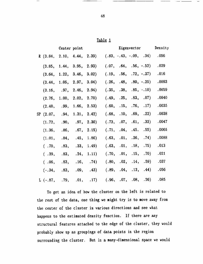
48

R (3.84,

(3.85,

(3.64,

(3.44,

(3.16,

(2.76,

(2.40,

SP (2.07,

(1.72,

(1.36,

(1.01,

( .70,

( .39,

( .06,

(-.34,

L (-.87,

Table 1

Center point Eigenvector Density

2.10, 4.44, 2.39) (.83, -.43, -.09, .34) .056

1.44, 3.95, 2.93) (.07, .64, .56, -.52) .029

1.22, 3.46, 3.02) (.19, .56, .72, -.37) .016

1.05, 2.97, 3.04) (.26, .48, .80, -.25) .0093

.97, 2.46, 2.94) (.35, .38, .85, -.10) .0059

1.00, 2.02, 2.70) (.49, .25, .83, .07) .0040

.99, 1.66, 2.53) (.60, .15, .76, .17) .0035

.94, 1.31, 2.42) (.68, .I0, .69, .22) .0038

.90, .97, 2.30) (.72, .07, .61, .32) .0047

.86, .67, 2.15) (.71, .04, .45..55) .0065

.84, .45, 1.86) (.63, .01, .26, .74) .0088

.83, .33, 1.49) (.63, .01, .18, .75) .013

.83, .24, I.II) (.70, .01, .15, .70) .021

.83, .16, .74) (.80, .02, .14, .59) .037

.83, .09, .43) (.89, .04, .12, .44) .056

.79, .01, .17) (.96, .07, .08, .26) .085

To get an idea of how the cluster on the left is related to

the rest of the data, one thing we might try is to move away from

the center of the cluster in various directions and see what

happens to the estimated density function. If there are any

structural features attached to the edge of the cluster, they would

probably show up as groupings of data points in the region

surrounding the cluster. But in a many-dimensional space we would

49

have to try a large number of directions in order that every

possible direction from the peak would be near one of the

directions we tried. Instead of trying to cover all possible

directions from the peak, we can use the data as a guide; that is,

we can look for data points on the fringe of the cluster, and

restrict our attention to the regions around those points. So I

computed the M-distance of each data point from the center of the

cluster, and I singled out those data points whose M-distance from

the center was between 3 and 4. These points would be on the

fringe of the cluster. I found 15 data points in this ellipsoidal

shell surrounding the cluster. For each one, I tried a window

centered at that point. Six of the 15 points are near each other

and near the center line of the bar described above, so they seem

to be part of the bar from the saddle point to the peak. Windows

at each of the other nine of these points showed that the density

at each point was very low, and none of them seemed to be part of a

new feature. So I concluded from this experiment that the cluster

on the left is at the end of a peninsula, which consists of the

curved bar described above. Also, as I noted above, the bar curves

into the long axis of the cluster on the left.

flUTLIERS AND MOREFEATURES

We will now look for outliers, that is, data points not

associated with any of the features found so far. Using the two

definitions of the M-distance given in Section 4, we can determine

which data points are associated at the 957 level with one of the

clusters we found above, or with the bar joining them. The number

5O

of data points associated with each cluster was given earlier. A

data point is associated with the bar if, for at least one of the

center points representing the bar, the data point satisfies the

two conditions stated in Section 4: M-distance to the estimated

center line below the cutoff value, and x* near the center point.

Various numbers of data points are associated with each of the

center points for the bar; for example, the number associated with

the saddle point is 46. Many data points are associated with more

than one center point. For each data point, I did the computations

for each of the 17 center points representing the features found so

far. The number of data points that are not associated at the 95Z

level with any of the features is 58 out of 634, or 9Z. If a data

set consisted of features with truly Gaussian shapes, the

proportion of outliers should be somewhere near 5Z. (I repeated

these computations using as cutoff values the upper IZ points of

the chi-square distribution, in order to find the number of data

points not associated at the 99Z level with any of the features.

The number of outliers at this level is 28 out of 634, or 4Z.)

If there are features in the data that we have not yet found,

then some of the apparent outliers should be grouped together. I

then did cross-tabs of the 58 outliers at the 95Z level, based on

various pairs of variables, to try to find possible concentrations

of data points. A few apparent groupings were visible in some of

the cross-tabs. By comparing those cross-tabs with the

corresponding cross-tabs for all 634 data points, I could see that

some of these groupings seemed to be near the edges of the clusters

I had already found. I went through the data set to find out which

51

data points were involved in these groupings of outliers, and I

then tried windows centered at some of those points. (These window

computations were based on all of the data, not just on the

outliers.) For some of the points there were too few nearby data

points to draw any conclusions. One of the points seemed to be

near a bar, so I moved toward the apparent center line, and then I

moved several steps along the estimated center line of the bar, in

the direction of increasing density. I used windows with WSD = 1

to explore this bar. Following along the bar led me to the broad

cluster on the right. Following the bar in the other direction led

to lower and lower densities, until finally the bar seemed to

dissipate. So the bar appears to be like a "finger" protruding

from the cluster, but in a different direction than the bar leading

to the saddle point. I chose four points along the estimated

center line to be the representative center points for the bar.

Table 2 gives the information for these four points, after

repeating the center point given in Table 1 for the cluster on the

right (marked "R"). Note that the direction of the bar is very

close to the direction of the long axis of the cluster; in fact,

the bar seems to be an extension of that long axis. Of the 58

original outliers, 20 are associated at the 95Z level with this

bar.

The cross-tabs also showed that there are five data points (on

the far left in Figure 1) with extremely small values for the first

infrared variable. They might be considered a cluster, or a small

bar, or perhaps two smaller clusters; there are too few points here

to tell. I called them a bar, and I chose the point

52

(-4.90, .46, -.09, -.19), which is roughly in the middle of these

five points, to be a center point to represent this bar. The

estimated center line of the bar is nearly parallel to the first

coordinate axis. (The WSD used was .8.)

Table 2

Center point Eigenvector Density

R (3.84, 2.10, 4.44, 2.39) (.83, -.43, -.09, .34) .056

(2.81, 2.63, 4.43, 2.04) (.86, -.44, .04, .26) .031

(1.61, 3.13, 4.30, 1.88) (.91, -.39, .12, .10) .020

( .32, 3.63, 4.14, 1.86) (.93, -.35, .10, .02) .017

(-.61, 3.77, 4.16, 1.76) (.97, -.21, .01, .09) .010

We now have a total of 22 center points to represent the

various features we have found. I ran through the data set again,

to look for outliers in terms of these features. The number of

outliers, that is, data points not associated at the 95_ level with

any of the features represented by these 22 center points, is 33

out of 634, or 5_. (I then repeated the computations at the 99_

level. The number of outliers at this level is 19 out of 634, or

3_.) I looked at several cross-tabs of the 33 outliers at the 95_

level, and there were no noticeable concentrations of points. I

conclude from this that we have found all the structural features

we can find in this set of 634 data points.

A SECOND SAMPLE

All of the results above are based on a random sample of one

tenth of the IRAS data set. In order to get an idea of the

53

variability of the estimates due to sampling error, I chose a

second random sample of 634 data points from the data set. For

this sample I selected every tenth data point, beginning with the

sixth. The two samples have no data points in common. Instead of

exploring this sample independently of the first sample, I assumed

that it would contain the same structural features as those found

in the first sample, but that their estimated parameters would be

so[ewhat different. I then computed the estimated parameters for

those features, based on the data in the second sample. For

consistency I used Ganssian windows of the same size as those used

for the features in the first sample. Since the locations of the

features are somewhat different in the second sample, I moved the

window centers to these new locations before estimating the shapes

of the features.

The results for the second sample are generally in agreement

with the results given above. For example, for the cluster on the

left, the center is at (-.75, .74, .05, .29) instead of

(-.87, .79, .01, .17), the estimated density at the center is .11

instead of .085, and the cluster mass is .16 instead of .17. The

eigenvectors defining the principal axes (especially the first

two), and the standard deviations along the axes, are similar to

those found before. For the broad cluster on the right, the

results are even closer to those found earlier, since a larger

amount of the data is involved in this cluster. The results for

the narrow cluster embedded in the broad cluster are not quite as

close. In particular, the eigenvectors are different fro[] those

found before (although there are some similarities), indicating

54

that the shape of the narrow cluster is different in the second

sample. This is probably because it is embedded in the broad

cluster, and there is really no clear distinction between the two.

In a sense, my description of the data in this region as two

Ganssian clusters is a matter of convenience. The estimated

parameters for the other features are generally similar to those

found earlier.

6. CONCLUSION

As a result of our exploration, we can describe the data set

as consisting of a broad cluster (on the right in Figure 1) with a

narrow cluster embedded in it, another cluster (on the left), and a

curved bar joining them. This bar has a saddle point, not quite at

the point with the lowest estimated density, but close to it. I

also found a "finger" protruding from one cluster, and a small

group of data points off to one side (on the far left). Each of

these features was described quantitatively. For each cluster I

gave two estimates of the proportion of the data set that was

involved in the cluster; these estimates were roughly in agreement

with each other. About 57 of the data points were called outliers.

My general strategy was to begin with an overall look at the

data, then to try relatively large Gaussian windows, and to follow

that with smaller windows. I looked first for clusters, or local

maxima, since they are relatively easy to find. Then, to see how

the clusters were related, and to explore other parts of the data,

I looked for saddle points and bars. I could also have searched

55

for more complex structures, such as essentially two-dimensional

concentrations of data points, but the data set did not seem to

have any such features. I usually moved around in the space by

moving the window center along the eigenvectors just found. By

doing so, I could move toward a peak or toward the center line of a

bar, or I could follow along a center line. I also used cross-tabs

as a guide, since it is often useful to have a picture to look at.

But I did not draw conclusions from them because such projections

may obscure some aspects of the structure of the data. I tried to

use strategies that could be used in any number of dimensions. For

example, to see how the cluster on the left was related to the

other parts of the data, I used the M-distance to define an

ellipsoidal shell about the cluster, and I looked at the data

points lying in that shell. I also used cross-tabs of outliers to

search for other possible features.

To obtain numerical estimates of the shape of a feature, I

used a window centered at the local maximum in the case of a

cluster, or at a point on the estimated center line in the case of

a bar. Since there is no "best" window size to use, and since the

estimates depend on the window size, these estimates are "soft"

numbers. However, if the estimates are relatively insensitive to

small changes in the window size, we can be confident that we are

looking at a real feature. I do not have rules for choosing a

window size, or for deciding whether a feature that appears to have

some internal structure (such as the broad cluster on the right)

should be described as more than one feature. Any such rules would

entail making additional assumptions about the data. I prefer to

56

leave that to the judgment of the user, who can then be guided by

his or her own knowledge, assumptions, or hypotheses about the

data.

My purpose in exploring a set of data is to find a way of

describing its structure so that we can understand it and think

about it. To this end, I have given some examples of structural

features that we might find in a set of data, some strategies for

searching for them, and some ways to describe them. Because of its

simplicity and generality, the method of Gaussian windows is a

useful tool for this purpose.

I would like to thank Peter Cheeseman of RIAC$ for providing

me with the IRAS data set, and Pentti Kanerva of RIACS for a

careful reading of a draft of this paper.

57

REFERENCES

Chambers, J., Cleveland, W., Kleiner, B., and Tukey, P. (1983),Graphical iethods for Data AnalFsis, Pacific Grove, CA: WadsworthBrooks/Cole.

Cheeseman, V., Kelly, J., Self, M., Stutz, J., Taylor, W., andFreeman, V. (1988), AUTOCLASS: A Bayesian classification system. InProc. Fifth 1.ter,atio,al Co.fcre.ce o. lachi,e £ear, i,9, pp.54-64. Morgan Kaufmann.

Cleveland, W., and McGill, M. (eds.) (1988), Dynamic Graphicsfor Statistics, Pacific Grove, CA: Wadsworth _ Brooks/Cole.

IRAS Catalogs and Atlases: The Poi,t Source Catalog (2nd ed.)(1985), General Printing Office, Washington, D.C.

Jaeckel, L. A. (1990), Gaussian windows: A tool for exploringmultivariate data. Technical Report 90.41, RIACS, _offett Field, CA

Jaeckel, L. A. (1991), Gaussian windows: A multivariateexploratory method. To appear in Proc. _3rd Symposi,m o, theInterface between Comp_ti,g Scie,ce a,d Statistics.

Morrison, D. F. (1990), I, ltivariate Statistical Methods (3rded.), New York: _cGraw-Hill.

Soifer, B. T., Beichman, C. A., and Sanders, D. B. (1989), Aninfrared view of the universe. Am. Sci. 77: 46-53.

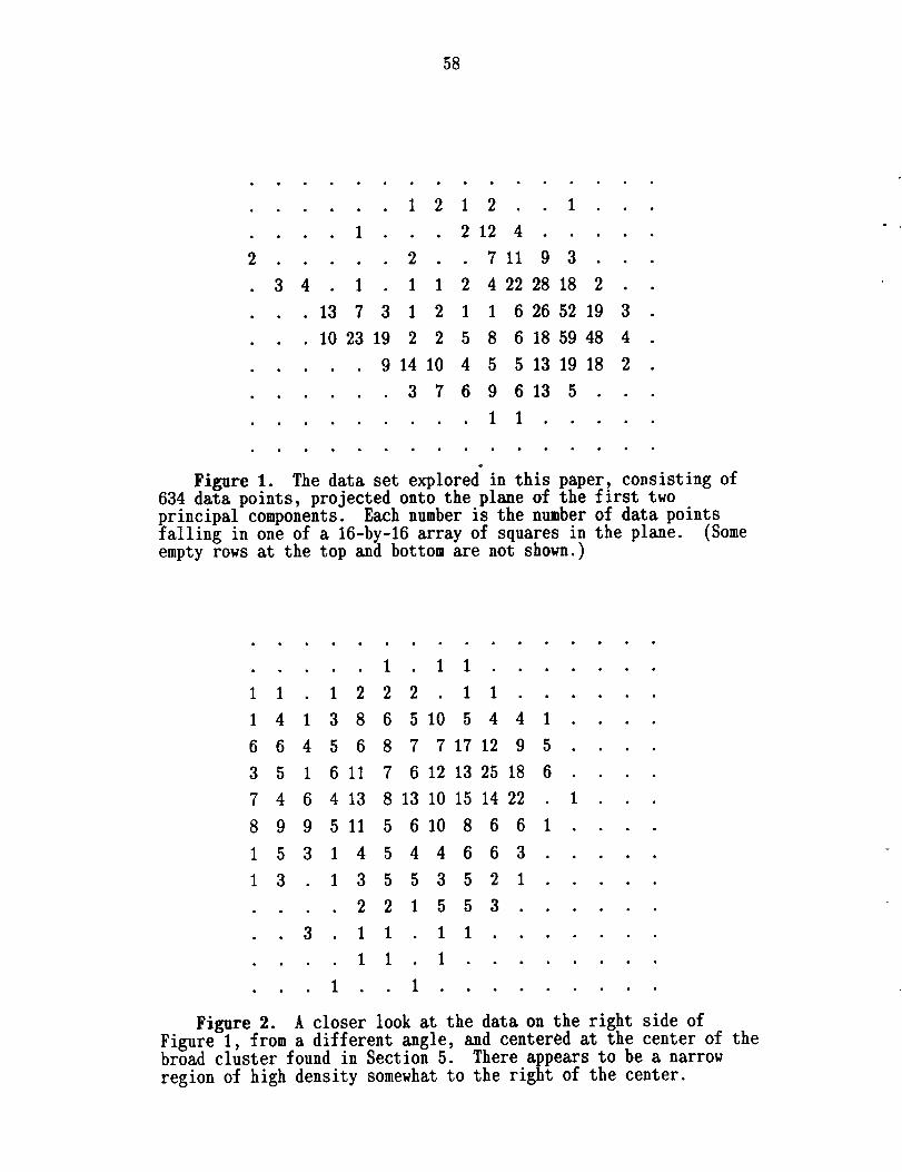
58

I

3 4 . 1

1 2 1 2 . 1

• 2 12 4

2 . 7 11 9 3 . .

1 1 2 4 22 28 18 2 .

• 13 7 3 1 2 1 1 6 26 52 19 3

I0 23 19 2 2 5 8 6 18 59 48 4

• 9 14 I0 4 5 5 13 19 18 2

• • 3 7 6 9 6 13 5

• . • I I •

Figure I. The data set explored in this paper, consisting of

634 data points, projected onto the plane of the first two

principal components. Each number is the number of data points

falling in one of a 16-by-16 array of squares in the plane. (Some

empty rows at the top and bottom are not shown.)

• I 1 1 . .

1 1 1 2 2 2 1 1 .

1 4 1 3 8 6 5 10 5 4 4 1

6 6 4 5 6 8 7 7 17 12 9 5

3 5 1 6 11 7 6 12 13 25 18 6

7 4 6 4 13 8 13 10 15 14 22 I

8 9 9 5 11 5 610 8 6 6 1

1 5 3 1 4 5 4 4 6 6 3

1 3 1 3 5 5 3 5 2 1

2 2 1 5 5 3 .

3 1 I I 1 .

1 I . I

• 1 . I . . •

Figure 2. A closer look at the data on the right side of

Figure 1, from a different angle, and centered at the center of thebroad cluster found in Section 5. There appears to be a narrow

region of high density somewhat to the right of the center.