User Guide (Windows and Macintosh)chem-is-try.us/class/ap/supplement/odyssey_v4/USER GUIDE...1 WORKING WITH Odyssey: THE ESSENTIALS 1.1 Welcome to Odyssey Odyssey is a content-rich

WAVEFUNCTION

Wavefunction, Inc.18401 Von Karman Avenue, Suite 370

Irvine, CA 92612 U.S.A.www.wavefun.com

Wavefunction, Inc., Japan Branch Office3-5-2, Kouji-machi, Suite 608

Chiyoda-ku, Tokyo, Japan [email protected] • www.wavefun.com/japan

User Guide (Windows and Macintosh)

Copyright © 2012 by Wavefunction, Inc.

All rights reserved in all countries. No part of this book may be reproduced in any form or by any electronic or mechanical means including information storage and retrieval systems without permission in writing from the publisher, except by a reviewer who may quote brief passages in a review.

ISBN 1-890661-39-2

Printed in the United States of America

CONTENTS

1. Working with Odyssey: The Essentials

1.1 Welcome to Odyssey .................................................................1 1.2 Manipulating Molecular Samples .................................................1 1.3 Working with Odyssey Content ................................................2

2. Working with Odyssey: The Complete Manual

2.1 General Operation .........................................................................5 2.1.1 Screen Layout ...................................................................5 2.1.2 Odyssey Icons ...............................................................5 2.1.3 Toolbar ..............................................................................6 2.1.4 Tabs ...................................................................................7 2.1.5 Mouse Functions ...............................................................7 2.1.6 Page Refresh/Reload .........................................................9 2.1.7 Working Without the Text Panel* ......................................9 2.1.8 Projector Friendly Colors* ................................................9 2.1.9 Hiding the Status Bar ......................................................10 2.1.10 Full Screen Mode ............................................................10 2.1.11 Annotating .......................................................................10 2.1.12 Print Text Preview ...........................................................10 2.1.13 Printing ............................................................................10 2.1.14 Periodic Table .................................................................11 2.1.15 Right Clicks/Short-Cut Menus ........................................12 2.1.16 Copy and Paste ................................................................12 2.1.17 Instructor Content* ..........................................................12 2.2 Simulations and Samples ............................................................13 2.2.1 Starting and Stopping Simulations..................................13 2.2.2 Sequences of “Frames” ...................................................13 2.2.3 Switching Samples ..........................................................14 2.2.4 Moving a Selected Molecule within a Sample ...............14 2.2.5 Changing Chirality ..........................................................15

i

* Instructor’s Edition only

ii

2.2.6 Saving Samples ...............................................................15 2.2.7 Saving Screenshots of Samples ......................................16 2.3 Visualization ...............................................................................16 2.3.1 Styles ...............................................................................16 2.3.2 Hydrogen Bonds .............................................................19 2.3.3 Lone Pairs .......................................................................19 2.3.4 Dipole Arrows .................................................................19 2.3.5 Collisions ........................................................................19 2.3.6 Reactive Events ...............................................................20 2.3.7 Trails ...............................................................................20 2.3.8 Velocities .........................................................................20 2.3.9 Clipping Feature ..............................................................20 2.3.10 Charge Labels .................................................................21 2.3.11 Molecular Properties as a Color Value ............................21 2.3.12 Ribbon Displays ..............................................................22 2.3.13 Electron Density Displays ...............................................22 2.3.14 Centering and Resizing ...................................................23 2.3.15 Comparing Two Samples ................................................23 2.4 Properties ....................................................................................23 2.4.1 Measuring Physical Properties ........................................23 2.4.2 Changing System Parameters .........................................24 2.4.3 Changing Slider Limits ...................................................25 2.5 Plotting ........................................................................................25 2.5.1 Requesting Plots..............................................................25 2.5.2 XY Plots ..........................................................................26 2.5.3 Customizing XY Plots ....................................................29 2.5.4 Moving the Plot Legend ..................................................30 2.5.5 Speed, Kinetic Energy, and Dipole Distributions ...........30 2.6 Building Your Own Samples.......................................................31 2.6.1 General Building .............................................................31 2.6.2 Entry-Level Builder ........................................................34 2.6.3 Advanced Builder ...........................................................34 2.6.4 Solid Builder ...................................................................35 2.6.5 Peptide Builder ................................................................35 2.6.6 Nucleotide Builder ..........................................................36 2.6.7 Bulk Sample Builder .......................................................36 2.6.8 Adding Labels .................................................................38 2.6.9 Changing Chirality While Building ................................38 2.6.10 Energy Minimization ......................................................38 2.6.11 Name Structure ...............................................................39 2.6.12 Evaluate Structure ...........................................................39

2.7 Preferences ..................................................................................39 2.7.1 Setting the Text Size .......................................................39 2.7.2 Physical Units .................................................................40 2.7.3 Boundary Display Style ..................................................40 2.7.4 Hydrogen Bonds Style ....................................................41 2.7.5 Color Preferences ............................................................41 2.7.6 Reduced Graphics for Slower Machines .........................41 2.7.7 “Expert” Setting* .............................................................42 2.7.8 Systematic and Common Names ....................................43 2.7.9 Dipole Orientation ..........................................................44 2.7.10 Sound Effects ..................................................................44 2.8 Using Odyssey with Other Programs, Files, and Documents .44 2.8.1 Reading PDB, XYZ, SMILES, ChemDraw, and ISIS/Draw Files ...............................................................44 2.8.2 Compatibility with Wavefunction’s spartan ...............45 2.8.3 Using Odyssey with PowerPoint .................................45 2.8.4 Hyperlinking Individual Samples ...................................46 2.8.5 Hyperlinking Labs or Stockroom Pages/Windows** .......46 2.8.6 Hyperlinking Labs or Stockroom Pages/Macintosh*** ....47 2.8.7 Hyperlinking the Home Page ..........................................48 2.8.8 Suppressing the Windows Security Dialog** ..................49 2.8.9 Saving Odyssey Pictures .............................................50

3. Scientific Background

3.1 Molecules in Motion: The Basic Idea Behind Dynamic Simulations .................................................................................51 3.2 Calculation of Molecular Interactions ........................................53 3.3 Why Do Molecules of Liquids Sometimes Disappear? ..............55 3.4 Rigid Molecules and the Speed of Simulations ..........................56 3.5 Do the Calculated Properties Reproduce Experimental Data? ...56 3.6 Does Odyssey Assume Ideal Gas Behavior? ...........................57 3.7 Gravity in Odyssey ..................................................................57 3.8 Condensing Gases .......................................................................58 3.9 Liquids Won’t Freeze ..................................................................58 3.10 Density Doesn’t Change When Melting .....................................58 3.11 Molecules Don’t Dissociate ........................................................58 3.12 Ions Don’t Dissolve Across an Interface.....................................59 3.13 Identification of Hydrogen Bonds ...............................................59 3.14 Calculation of Enthalpies, Entropies, and Free Energies ............60

iii

* Instructor’s Edition only ** Windows only *** Macintosh only

4. Teaching Usage

4.1 Simulating the Liquid-Vapor Transition .....................................62 4.2 Incorporating Simulations into Presentations and Classwork ....62 4.3 Can Odyssey Be Used with Interactive Whiteboards? ............63 4.4 Annotating Pages ........................................................................63

5. Computer Questions and Troubleshooting

5.1 Graphics Performance .................................................................64 5.2 Running on Battery .....................................................................64 5.3 Graphics Hardware Acceleration* ...............................................64 5.4 Windows Operating System Requirements* ...............................65 5.5 Macintosh Operating System Requirements** ............................65 5.6 Differences Between Pre-Built and User-Built Samples ............65 5.7 Problems with Collision or Velocity Highlighting ......................65 5.8 Vapor Molecules Don’t Seem to Move Fast Enough ..................66 5.9 Creating File Associations* .........................................................66 5.10 Suppressing the “Blocked Content” Message Bar when67 Printing PDF-Formatted Worksheets* .........................................67 5.11 Opening Saved Models with “Drag and Drop” ..........................67 5.12 Importing From Other Modeling Programs ................................67 5.13 Uninstalling the Windows Version* ............................................68

Index ..........................................................................................................69

iv

* Windows only ** Macintosh only

1

WORKING WITH Odyssey: THE ESSENTIALS

1.1 Welcome to Odyssey

Odyssey is a content-rich learning and simulation environment for molecular science. The software is designed to be used in two ways:

• Web-Style Browsing. Simply navigate through “pages” and follow “links”—No learning curve!

• Menu-Driven. Explore and visualize molecular systems with Odyssey’s powerful, yet easy-to-use graphical interface.

The next few pages explain everything you need to know to get started.

1.2 Manipulating Molecular samples

• Start Odyssey via its icon on the desktop or in the “Programs” menu (Windows) or via the Applications folder (Macintosh). Odyssey opens to its home page.

• To maximize screen size, click on the “Maximize” icon in the upper right hand corner of the page (Windows) or upper left corner (Macintosh).

• Click on Molecular Stockroom.

• Choose any of the topics.

2

• With a molecular sample displayed, verify the following mouse functions:

• Click and drag with the left mouse button to rotate the sample.

• Click and drag with the right mouse button to translate the model.

• Use the mouse scroll wheel to zoom in and out. (If your mouse does not have a scroll wheel, hold SHIFT and then right-click and drag.)

• You can start a physics-based simulation by clicking on the icon below the sample. Click on the icon again in order to stop the simulation.

• Exit by clicking on the “Close” icon for the page (in the Windows version, the icon appears on the right hand side of the tab). Closing the page takes you back to the Molecular Stockroom page.

• Click on HOME (the far left tab) to go back to Odyssey’s home page.

1.3 Working with Odyssey Content

• From Odyssey’s intial page, click on Molecular Labs.

• Choose one of the topics that is of interest to you.

3

• The text is interspersed with blocks of “radio buttons” and other webpage-style controls. Clicking on these controls will trigger sample and visualization changes—try this out.

• Close the experiment by clicking on the “Close” icon for the page (in the Windows version, the icon appears on the right hand side of the tab). This takes you back to the Molecular Labs page.

• Choose another topic and try out the webpage-style controls.

• Without closing this page, go back to the Molecular Labs page by clicking on the LABS tab.

• Choose another topic.

4

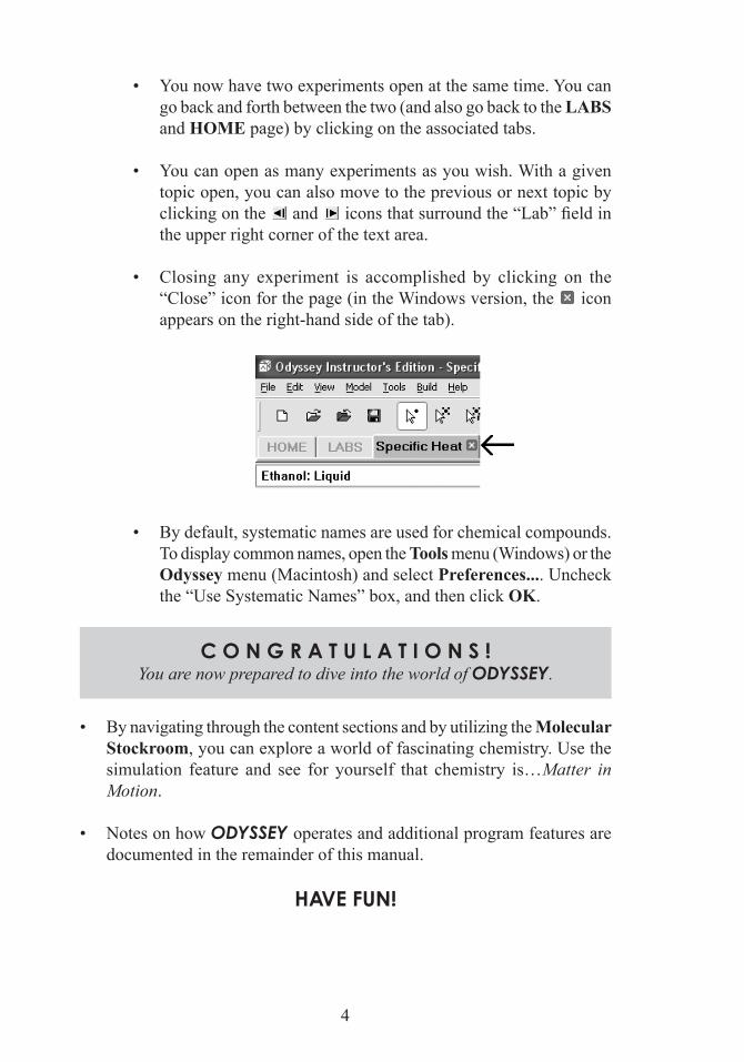
• You now have two experiments open at the same time. You can go back and forth between the two (and also go back to the LABS and HOME page) by clicking on the associated tabs.

• You can open as many experiments as you wish. With a given topic open, you can also move to the previous or next topic by clicking on the and icons that surround the “Lab” field in the upper right corner of the text area.

• Closing any experiment is accomplished by clicking on the “Close” icon for the page (in the Windows version, the icon appears on the right-hand side of the tab).

• By default, systematic names are used for chemical compounds. To display common names, open the Tools menu (Windows) or the Odyssey menu (Macintosh) and select Preferences.... Uncheck the “Use Systematic Names” box, and then click OK.

C O N G R A T U L A T I O N S !You are now prepared to dive into the world of Odyssey.

• By navigating through the content sections and by utilizing the Molecular Stockroom, you can explore a world of fascinating chemistry. Use the simulation feature and see for yourself that chemistry is…Matter in Motion.

• Notes on how Odyssey operates and additional program features are documented in the remainder of this manual.

HAVE FUN!

5

WORKING WITH Odyssey:THE COMPLETE MANUAL

2.1 General Operation

2.1.1 screen Layout

To change the size of the tiles for the Sample, Text, Properties, and Plots/Build/Cell areas:

• Position cursor on boundary between two tiles, click, and drag.

2.1.2 Odyssey Icons

Simulations/Sequences: Properties:

Start Add Property to List

Stop Remove Property from List

Step Forward Hide Properties Panel

Step Reverse

Change Frame

6

Experiments:

Next Experiment

Previous Experiment

Text:

Page Refresh

Notes

Close Experiment or Stockroom Page Hide Instructor Comments and Answer Key*

Plots:

Add Plot Edit Plot

Remove Plot Clear Plot (Erase Datapoints)

Record Datapoint Hide Plots Panel

Other:

Properties Table Projector Friendly Colors*

Plots Pane Hide Text Panel*

Electrons Periodic Table

Compare Clear Answers and

Snapshot

2.1.3 toolbar

To display a toolbar with icons for commonly used operations:

• From the View menu, select Toolbar.

Build:

Build Mode Add Delete Make Bond Break Bond Simulation Cell Minimize Set Labels Evaluate Structure Name Structure Molecular Formula


Annotations

7

The size of the toolbar icons can be changed:

• From the Tools menu (Windows) or from the Odyssey menu (Macintosh), select Preferences.

• Choose among Text Only, Small Icons, Medium Icons, or Large Icons.

Note: In the Macintosh version, a page with a molecular sample must be open for the menu item to be available. In the Windows version, the toolbar can be (temporarily) moved to anywhere on the screen by dragging the “ridge” at its extreme left end.

2.1.4 tabs

Odyssey employs the tabbed interface of newer web browsers:

• Whenever you open an item in Home, Molecular Labs or in the Molecular Stockroom, a new tab is created. You can go back and forth between tabs as desired.

• Generally, as many experiments/samples as desired can be simultaneously open.

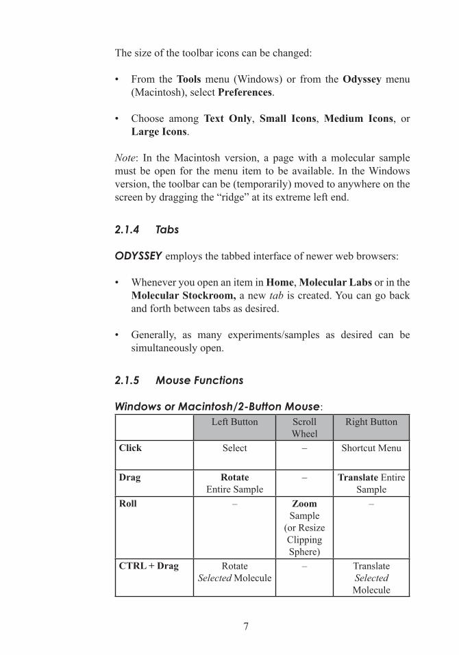
2.1.5 Mouse Functions

Windows or Macintosh/2-Button Mouse:Left Button Scroll

WheelRight Button

Click Select – Shortcut Menu

Drag Rotate Entire Sample

– Translate Entire Sample

Roll – Zoom Sample

(or Resize Clipping Sphere)

–

CTRL + Drag Rotate Selected Molecule

– Translate Selected Molecule

8

CTRL + Double- Click2

+ Double- Click3

Invert Stereocenter

– –

SPACE BAR + Drag

Rotate Selected Bond1

– Stretch Selected Bond1

In Build Mode Only:Click Perform Build

Action– –

Double-Click Insert New – –1 Red wrap-around arrow indicates selection 2 Windows 3 Macintosh

Less Important:SHIFT + Drag4 Z-Axis Rotate of

Entire Sample– Zoom Sample (or

Resize Clipping Sphere)

Left Button + Right Button + Drag

Define Area (Style Changes Only)

4 Drag up and down

Macintosh/1-Button Mouse:Click SelectCTRL + Click Shortcut MenuDrag Rotate Entire Sample + Drag Translate Entire SampleSHIFT + + Drag1 Zoom Sample

(or Resize Clipping Sphere)CTRL + Drag Rotate Selected MoleculeCTRL + + Drag Translate Selected Molecule + Double-Click Invert StereocenterSPACE BAR + Drag Rotate Selected Bond2

SPACE BAR + + Drag3 Stretch Selected Bond2

In Build Mode Only:Click Perform Build ActionDouble-Click Insert New

Less Important (all models)4:SHIFT + Drag1 Z-Axis Rotate of Entire Sample1 Drag up and down 2 Red wrap-around arrow indicates selection 3 First depress SPACE BAR, then depress 4 “Define Area” (for style changes) is not available

9

2.1.6 page refresh/reload

Click on the icon next to the page title for a full refresh of an experiment. The action refreshes all samples of the current experiment. (Experiments in other tabs are unaffected by a refresh.)

A Reload option is also available in the shortcut (right-click) menu when the cursor is within the text area. However, the effect of this reload is limited: It only refreshes the HTML of the current page, i.e., it does not refresh the molecular samples.

2.1.7 Working Without the text panel*

To hide the text panel of the current page (the toolbar must be shown):

• Click on the icon.

The setting will be applied to all pages in the current session (but will not carry over to the next session).

2.1.8 projector Friendly Colors*

To switch to a background color scheme that is more suitable for classroom projection than the default black background color (the toolbar must be shown):

• Click on the icon.

The setting is applied throughout the current session. Future sessions, however, will start with the normal (black background) color scheme.

2.1.9 Hiding the status Bar

The status bar at the bottom of the window can be temporarily hidden:

• In the View menu, uncheck Status Bar.


10

2.1.10 Full screen Mode

Odyssey can be put into presentation-style full screen mode:

• From the View menu, select Full Screen.

To exit full screen mode:

• In the View menu, deselect Full Screen.

2.1.11 annotating

To annotate an Odyssey page:

• Click on the icon at the top of the text panel. This opens a Notes page that accepts any “text” that is entered.

• Return to the originating page by clicking on the SAVE+CLOSE link at the bottom of the Notes page.

The annotations for a given page are retained by the computer and will be shown whenever you return to the Notes page later.

2.1.12 print text preview

Printable text items can be previewed:

• Choose Print Text Preview in the File menu.

2.1.13 printing

Printing of Sample Snapshots:

• From the File menu, select Print Sample Image....

Printing of Plots:

• Select the plot (it has a red border around it if selected).

• From the File menu, select Print Active Plot....

11

Printing of Text Panel:

• From the File menu, select Print Text....

Printing the Properties Table:

Use the computer’s screen-capture facility (many machines have a special “Print Screen” key):

• Paste the screen shot into any picture editing program.

• Using the editing features of the picture editing program, crop the screenshot around the Table of Properties.

• Print the cropped picture directly from the picture editing program.

Printing of the Entire Screen:

• Use the screen-capture facility of your computer—many machines have a special “Print Screen” key.

• Paste the screen shot into any picture editing program.

• Print directly from the picture editing program.

2.1.14 periodic table

To display a periodic table of the elements:

• From the Tools menu, select Periodic Table . . .

The periodic table can be displayed with the following color overlays:

• Default: Odyssey atom colors

• Coloration by standard state (gas, liquid, or solid)

• Coloration by metallic character (metallic, semimetallic, or nonmetallic character)

12

• Coloration by valence electron configuration (s/p/d/f blocks; noble gases)

2.1.15 right-Clicks/short-Cut Menus

To access short-cut menus (“contextual” menus):

• Right-click (shortcut menus are available in the sample and text areas)

2.1.16 Copy and paste

The clipboard is enabled (in the Edit menu, select one of three Copy options). This allows for easy export of pictures and data to Word documents, PowerPoint presentations, etc.:

• Screenshots can be retrieved from the sample area: Use Copy Sample Image

• Text strings can be retrieved from the text area: Use Copy Selected Text

• Plots can be retrieved from the plots area: click on the plot, then select Copy Active Plot

2.1.17 Instructor Content*

For any individual page, the visibility of instructor comments and the answer key can be toggled on and off by clicking on the icon at the top of the text panel.

To automatically show the instructor comments for all pages:

• From the Tools menu, (Windows) or the Odyssey menu (Macintosh), select Preferences...

• Check Show Instructor Content by Default.


13

2.2 simulations and samples

2.2.1 starting and stopping simulations

Most molecular samples can be subjected to molecular dynamics simulations (= physical simulations in time):

• Use the / button below the molecular sample in order to initiate and stop the simulations.

• Use the button in order to advance in small time increments.

• Use the button in order to go backwards in time in small increments.

The choice of time step reflects the size of the system as well as expectations regarding the accuracy of such simulations. For large, user-built systems (>50 atoms) that have bonded hydrogen atoms, the timestep is initially set to 1 fs. For large user-built systems that contain no hydrogens, the time step is initially set to 2 fs and for user-built monatomic systems (such as noble gases), it is set to 5 fs. If simulations seem to progress with an occasional “slow-down” of all particle motion, this is due to automatic adjustments in the simulation procedure.

Note: The default time steps of user-built systems are chosen to allow for efficient simulations that advance quickly. For greater accuracy, and particularly to better resolve intramolecular vibrations, smaller time steps need to be chosen.

2.2.2 sequences of “Frames”

Some samples (particularly those with “surfaces”) can be viewed in a sequence that is not related to physical time:

• Use the / button below the sample to start and stop an animation of these sequences. Note that what is shown is not a physical simulation, but a simple animation of a number of prerecorded “frames”.

• Use the button to move one frame ahead in the sequence.

14

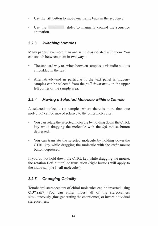
• Use the button to move one frame back in the sequence.

• Use the slider to manually control the sequence animation.

2.2.3 switching samples

Many pages have more than one sample associated with them. You can switch between them in two ways:

• The standard way to switch between samples is via radio buttons embedded in the text.

• Alternatively–and in particular if the text panel is hidden–samples can be selected from the pull-down menu in the upper left corner of the sample area.

2.2.4 Moving a selected Molecule within a sample

A selected molecule (in samples where there is more than one molecule) can be moved relative to the other molecules:

• You can rotate the selected molecule by holding down the CTRL key while dragging the molecule with the left mouse button depressed.

• You can translate the selected molecule by holding down the CTRL key while dragging the molecule with the right mouse button depressed.

If you do not hold down the CTRL key while dragging the mouse, the rotation (left button) or translation (right button) will apply to the entire sample (= all molecules).

2.2.5 Changing Chirality

Tetrahedral stereocenters of chiral molecules can be inverted using Odyssey. You can either invert all of the stereocenters simultaneously (thus generating the enantiomer) or invert individual stereocenters:

15

• To invert all of the stereocenters simultaneously, right click any of the atoms and choose Invert Molecule Chirality.

• To invert just one stereocenter, right click on the stereocenter and choose Invert Atom Chirality. Alternatively, double-click on the stereocenter while holding down the CTRL key (Windows or the key (Macintosh).

Note: Only tetrahedral stereocenters can be inverted, not octahedral stereocenters.

2.2.6 saving samples

The currently displayed sample can always be saved as an .xodydata file into locations outside of the Odyssey folder (the Odyssey folder is Read Only in order to preserve the integrity of the software):

• From the File menu, select Save Sample As....

• Navigate to the desired location, select a filename, and save the file.

• The saved sample is shown in a new tab.

The following restriction applies when saving samples:

• “Surface” information (Orbitals, Electron Density Distributions, Electrostatic Potentials, Polarity Maps) is not saved.

For export to Wavefunction’s program spartan, samples can be saved in the .spinput format. Note that all “simulation cell-specific” information (such as the bounding box) is lost when saving in this format.

For exporting to other programs, the SMILES connectivity format can be used. You must have the Instructor’s Edition and be in Expert Mode (See 2.7.7) to save in the SMILES format. Note that for charged species, the entire molecular charge will be assigned to a single atom.

16

2.2.7 saving screenshots of samples

Screenshots of molecular samples can be saved:

• From the File menu, select Save Sample Image As...

• Choose a file name and one of the following file types:

.jpg (compressed) - Windows and Macintosh

.png (compressed, no loss) - Windows and Macintosh

.bmp (uncompressed) - Windows only

• Save the graphics file to the desired location.

Tip: For best resolution, zoom in prior to saving the screenshot. In the Instructor’s Edition, you can furthermore hide the text panel using the corresponding toolbar icon.

The clipboard (Edit→Copy Sample Image) can also be used to export pictures.

2.3 Visualization

2.3.1 styles

Molecular samples can be displayed in a variety of styles that are best illustrated using an example:

• On the Molecular Stockroom page, find “Hydrogen Peroxide” (depending on the version of Odyssey either on its own page or as part of the Hydrogen Oxides page). Choose Hydrogen Peroxide as an Aqueous Solution.

17

• Try out the five styles, all available in the Style menu:

• The appearance of individual atoms can be customized:

• From the Edit menu, choose Select Atom (which is, incidentally, the default).

• Click on any atom. The atom becomes highlighted. From the Style menu, choose the desired style (e.g., Ball and Wire).

• Click on the background to deselect the atoms.

• The appearance of molecules can also be customized:

• From the Edit menu, choose Select Molecule.

• Click on one atom from one of the molecules (e.g., water). All atoms of the selected molecule become highlighted. From the Style menu, choose the desired style (e.g., Space Filling).


18

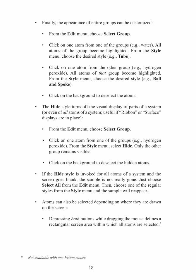
• Finally, the appearance of entire groups can be customized:

• From the Edit menu, choose Select Group.

• Click on one atom from one of the groups (e.g., water). All atoms of the group become highlighted. From the Style menu, choose the desired style (e.g., Tube).

• Click on one atom from the other group (e.g., hydrogen peroxide). All atoms of that group become highlighted. From the Style menu, choose the desired style (e.g., Ball and Spoke).


• The Hide style turns off the visual display of parts of a system (or even of all atoms of a system; useful if “Ribbon” or “Surface” displays are in place):

• From the Edit menu, choose Select Group.

• Click on one atom from one of the groups (e.g., hydrogen peroxide). From the Style menu, select Hide. Only the other group remains visible.

• Click on the background to deselect the hidden atoms.

• If the Hide style is invoked for all atoms of a system and the screen goes blank, the sample is not really gone. Just choose Select All from the Edit menu. Then, choose one of the regular styles from the Style menu and the sample will reappear.

• Atoms can also be selected depending on where they are drawn on the screen:

• Depressing both buttons while dragging the mouse defines a rectangular screen area within which all atoms are selected.*

* Not available with one-button mouse.

19

2.3.2 Hydrogen Bonds

To turn on hydrogen bond display (if such bonds are present in the sample):

• From the Style menu, select Hydrogen Bonds.

2.3.3 Lone pairs

To display a schematic representation of lone pairs (where applicable):

• From the Style menu, select Lone Pairs.

Note: The schematic visualization of lone pairs is not always available. Lone pairs are never available for noble gas-like unbonded atoms or ions.

2.3.4 dipole arrows

To turn on the display of molecular dipoles (if dipoles are present in the sample):

• From the Style menu, select Dipole Arrows.

Dipoles can be turned on selectively:

• Use Select Molecule or Select Group in the Edit menu (see the “Styles” section above for a demonstration of the “Select” feature) prior to turning on the dipole display.

2.3.5 Collisions

Display of collisions via “halos” can be turned on for gases, provided the physical density of the gas is not too large:

• From the Style menu, select Collisions, and then choose what type of collisions to display. The choices are Molecule-Molecule, Molecule-Wall, All or None.

20

2.3.6 reactive events

When reactions are allowed in the system, Odyssey can highlight the active reactions to make them easier to find.

• From the Style menu, select Reactive Events to toggle the highlighting of reactions.

2.3.7 trails

Molecular trails or “trajectories” can be graphically traced:

• From the Style menu, select Trails.

Trails can be turned on selectively:

• Use Select Molecule or Select Group in the Edit menu (see the “Styles” section above for a demonstration of the “Select” feature) prior to turning on the trails display.

2.3.8 Velocities

Molecular velocities can be displayed graphically for systems with low enough densities:

• From the Style menu, select Velocities.

Velocities can be turned on selectively:

• Use Select Molecule or Select Group in the Edit menu (see the “Styles” section above for a demonstration of the “Select” feature) prior to turning on the velocities display.

Note: This attribute is not available for higher density samples.

2.3.9 Clipping Feature

The display of many molecular samples can be greatly simplified by only displaying atoms that are close to a user-set “center.”

21

Using the clipping feature requires two steps:

• Setting the Clipping Center:

Right-click on an atom, and select Set Clipping Center.

• Choosing a Clipping Sphere Radius:

Select the clipping sphere by clicking on the sphere (selection is indicated by a color change). Use the usual zoom-in/zoom-out functionality to adjust the size of the clipping sphere (use the scroll wheel or drag the mouse with the right-mouse-button + SHIFT key depressed). Click on the background when done.

Once a clipping center has been set, the use of clipping can be toggled from the menu bar:

• From the Style menu, select Clipping.

2.3.10 Charge Labels

To turn on the display of charge labels:

• From the Style menu, select Charge Labels, and then choose either Net (Ionic) or Partial (Atomic).

2.3.11 Molecular properties as a Color Value

Molecules can be colored according to their instantaneous kinetic energy, dipole moment or instantaneous binding energy (the bonding energy of a molecule and the energy of interaction of a given particle with all its neighbors).

• From the Style menu, select Color by Property.

• In the submenu, choose from Translational Kinetic Energy, Binding Energy, Dipole Moment or None.

The color scale ranges from blue through white to red:

• Blue: small kinetic energy / very negative binding energy / small dipole moment magnitude

22

• White: intermediate values

• Red: large kinetic energy / less negative (or positive) binding energy / large dipole moment magnitude

As the simulation progresses, the numerical limits for defining the color scale are generally held constant. The range is never reduced; it is expanded if a smaller minimum or larger maximum is encountered. To display a particular range of values, open the Style menu, select Color by Property and then choose Customize.... If you click on the User-Defined check box, you can then set the low and high values used for the coloration. Each of the three properties has its own range.

2.3.12 ribbon displays

Proteins and nucleic acids that contain explicit residue information (this includes samples that have been built with Odyssey’s Peptide or Nucleotide builder as well as PDB files from the Protein Data Bank) can be displayed as “Ribbon” models with a visual indicator for the backbone of the molecule:

• From the Style menu, select Ribbons (if the entry does not appear in the menu, then the underlying file does not contain the necessary residue information), then choose what type of ribbon to display. The choices are Monochrome, By Secondary Structure, By Strand, and By Residue.

Note: Odyssey uses hidden data to determine the ribbon information. For some files (such as those that have been heavily modified) this information is unavailable and Odyssey cannot display the ribbons needed to highlight the backbone.

2.3.13 electron density displays

For systems with up to 30 atoms, Odyssey is capable of calculating a variety of electronic “surfaces”:

• Electron Density Surfaces, both for a high density isovalue (Inner Surface) and a low density isovalue (Outer Surface)

• Polarity Maps (Electrostatic Potential Maps)

23

To generate surfaces and change their appearance:

• From the Electrons menu, select the name of the surface, e.g., Polarity Map.

• In the lower half of the menu, choose among Solid, Transparent, Mesh, or Dots.

2.3.14 Centering and resizing

To center molecular samples:

• From the Edit menu, select Center.

To resize molecular samples:

• From the Edit menu, select Resize.

2.3.15 Comparing two samples

Two samples can be shown side-by-side for the purpose of comparing them:

• From the View menu (or using the Compare icon), select Side-by-Side. If you are on a page with multiple samples, you can pick one of them from the list. If there is no list (or if the list does not include what is desired), select Search for more systems... Use the search box to identify the desired sample, then click OK.

• To facilitate comparisons where samples are “shown on the same footing,” the second sample is initially displayed with the zoom setting and style taken from the first sample. You may have to zoom in or out in order to get the desired view.

• One of the two samples always has the focus―it is indicated via a red frame. You change the focus by simply clicking on the sample’s background.

• A sample can even be compared “to itself” (unless it was built from scratch). What this means is that a copy of the first sample is created. After creation of the copy, the two samples exist independently and can be manipulated separately.

24

By default, only one sample at a time (the one with the red frame around it) can be subjected to simulations. However, the two samples can also be synchronized and run at the same time:

• From the View menu (or using the Compare icon), select Synchronize: The two Stop/Go simulation buttons below the two samples get replaced by one such button in the middle.

Synchronization only applies to the simulation capability―any visualization changes still only apply to the sample with the focus.

2.4 properties

2.4.1 Measuring physical properties

To query the numerical values of physical properties:

• From the View menu, select Properties.

• From the Add Property menu (in the lower left corner), select the desired property, such as Atom→Electronegativity.

• If a selection is required, then this is indicated in the column to the right of the properties list; e.g., adding Mole Fraction to the list necessitates a Select Group action.

Additional properties are added to the panel via the “ ” button.

• If a property is added to the table, its numerical value will instantly be displayed (if it is a “system” property that does not require any selection and if the value is available without further need for simulation).

• Selections apply to the active property at any given time: You make a property “active” (property field background turns red to indicate selection) by selecting it in the list.

• If a property value is “Pending,” then a simulation is required in order to calculate its value. The calculated number is filled in automatically as soon as it becomes available. When applicable, a

25

proper selection (such as two atoms for a distance measurement) must have been made.

Some properties have both averaged and instantaneous values. To change between these, first select the property by clicking on its name. If that property can be changed between averaged and instantaneous, a button ( ) will appear to the right of the property name. Clicking on this button will let you choose between Averaged and Not Averaged.

Only properties that apply to the given molecular sample are displayed, e.g., the entry Mole Fraction is absent for one-component systems or individual molecules.

To delete or hide property information:

• Any individual property can be removed from the list by selecting it (which makes it the active property) and by then clicking on the icon to the right of “ .”

• The entire “Properties” panel can be hidden by clicking on the icon (“local close button”) in the upper right hand corner of

the panel. The operation only hides the panel, i.e., it does not erase the property information.

2.4.2 Changing system parameters

System parameters of bulk matter samples can often be changed. For these properties, a slider will appear when you select the property. The property can be changed by adjusting the slider, even while the simulation is in progress. (In the Windows version only, the value can also be changed with vertical spinners.) Some of the properties that can be changed are:

• Temperature:

Add Thermodynamics→Temperature to the list of properties.

• Volume:

Add Thermodynamics→Volume to the list of properties.

26

• Number of Molecules/Atoms in One-Component Systems:

Add System→Total Number of Molecules (or System→Total Number of Atoms if monoatomic) to the list of properties.

• System Composition in Multi-Component Systems:

Add Composition→Number of Molecules (or Composition →Number of Atoms if monoatomic) to the list of properties. Then select any group.

Note: In two-dimensional systems, Area replaces volume.

2.4.3 Changing slider Limits

Built-in limits for temperature, volume, and composition sliders can be overwritten by explicitly requesting a property value outside of the default range:

• Click the numerical value field for the property and enter your desired value (excluding units).

Note: The limits of the corresponding slider are updated to include the newly requested value.

2.5 plotting

2.5.1 requesting plots

Odyssey can generate numerous types of XY plots. In addition, Odyssey reports three kinds of histograms (for the molecular speeds, molecular kinetic energies, and dipole moments).

To request a plot:

• From the View menu, select Plots.

• Individual plots are added to the panel via the “ ” button. You can add as many plots to the plots panel as you wish.

27

To clear a plot (= erase the data points):

• Click on the icon at the top of the plots panel.

To delete or hide plots:

• Any plot can be removed from the “Plots” panel by selecting it (= making it the active plot) and then clicking on the icon to the right of “ .”

• The entire “Plots” panel can be hidden by clicking on the icon (“local close button”) in the upper right hand corner of the panel. The operation only hides the panel, i.e., it does not erase the plot data.

2.5.2 Xy plots

Most plots are obtained by actively recording measurements as a simulation is in progress or by following the time evolution of a selected property over the course of a similation. Examples include:

• Total Energy as a function of Temperature

• Potential Energy as a function of Time

• Entropy as a function of Temperature

More complicated plots that incorporate data from multiple samples can also be generated (see Advanced options below).

To generate an XY Plot (once the plot pane is up, see preceeding section):

• In the Plots panel, select the “ ” button.

Examplesof XY Plots

28

• From the list, select XY Plot….

• Select the property for the X Axis and select the property for the Y Axis.

• You can choose Use Average and What to plot (the value, 1/value, log(value)) or use the defaults.

• Additional options can be invoked by clicking Advanced. Depending on the sample and X/Y properties chosen, the following may be available:

• “Allow for multiple curves, with one curve for each sample”

This option will generate a plot with multiple curves. Each curve corresponds to a sample and recording data will add datapoints to the curve for the selected sample. The sample can be changed by either choosing among the samples in the text or by using the drop-down menu above the sample. Only available for experiments with multiple samples.

• “Different samples are datapoints in a single curve”

This option generates a plot with each sample corresponding to a single datapoint. The record button is not active. If you choose this plot type, you may need to run each sample briefly to get that sample’s datapoint to appear. The datapoint for the current sample is shown in yellow. As you run any of the samples, the datapoint that corresponds to that sample will move as the property values change. This is only available for experiments with multiple samples.

Example of a plot where

different samples are datapoints in a

single curve

29

• “Allow for multiple curves that differ in the following parameter”

This option generates a plot that can have multiple curves. After choosing this option, you must select a property from the list. All of the datapoints that you record with the same value of this parameter will be in one curve. If you change the parameter property, the new datapoints you record will be in a separate curve on the same plot.

Odyssey automatically assigns different symbols for datapoints of different parameter values.

• “One curve”

This option will generate a plot where each datapoint that is recorded is placed in a single curve. This is only available for experiments that have a single sample.

• Click Next.

• Choose among Scatter Plot, Linear Fit, Point-to-Point, and Smoothed Fit.

• If the axis property requires a selection, a rectangle will appear near the axis label. Click on this rectangle (to make it active) and then select the desired entities in the model.

While the simulation is in progress, click on the icon (“Record”) in order to generate datapoints. Typically this is done while systematically varying one of the two properties (such as Temperature or Volume). The record button does not “light up” until sufficient data have been accumulated to allow for measurement. This may take several seconds or more for a given simulation.

Example of an XY plot with a parameter

30

Odyssey autoscales the X and Y axis ranges based on the minimum and maximum values that are encountered. If one of the limits exceeds the previous value, the range is updated.

Note: The resolution of plots with “Time” as the independent variable is not sufficient to capture extremely fast fluctuations, such as the potential energy (or intramolecular geometry) of hydrogen-containing flexible molecules.

2.5.3 Customizing Xy plots

To change the title, curve fit, or plotting function of a plot:

• Make the plot “active” by clicking on it.

• Bring up the “Plot Edit” panel by clicking on the icon at the top of the plots panel.

• Several items can be customized:

• Plot Title

• Labels for the X and Y Axis

• Grid Lines for the X and Y Axis

• Explicit Range for the X and Y Axis

• Curve Fit of None, Point-to-Point, Smoothed Fit, or Linear Fit.

• Plotting function (e.g. X, 1/X, log(X))

2.5.4 Moving the plot Legend

To move the legend of plots (e.g., in order to expose datapoints “hidden” behind the legend):

• Position the cursor on the legend, click, and drag.

2.5.5 speed, Kinetic energy, and dipole distributions

Three kinds of histograms can be generated:

31

• Speed Distribution: A histogram showing the probability of encountering speed values.

• Translational Kinetic Energy Distribution: A histogram showing the probability of encountering translational kinetic energy values.

• Dipole Distribution: A histogram showing the probability of encountering dipole moment values.

To generate a histogram:

• From the View menu, select Plots.

• From the list of “Plots” (upper left corner of the Plots panel), select either Speed Distribution, Translat. Kinetic Energy Distribution, or Dipole Distribution.

The appearance of a histogram can be customized:

• Make the histogram “active” by clicking on it.

• Bring up the “Plot Edit” panel by clicking on the icon at the top of the plots panel.

• Items available for customization include:

• The histogram Title.

• The histogram Style: Bar or Line.

• The Samples setting: The default is Single. If set to Multiple, histograms for multiple samples (then automatically forced to be in the Line style) can be shown in the same plot.

Example of a Histogram

(Speed Distribution)

32

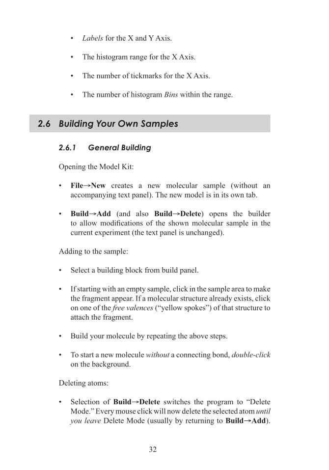
• Labels for the X and Y Axis.

• The histogram range for the X Axis.

• The number of tickmarks for the X Axis.

• The number of histogram Bins within the range.

2.6 Building your Own samples

2.6.1 General Building

Opening the Model Kit:

• File→New creates a new molecular sample (without an accompanying text panel). The new model is in its own tab.

• Build→Add (and also Build→Delete) opens the builder to allow modifications of the shown molecular sample in the current experiment (the text panel is unchanged).

Adding to the sample:

• Select a building block from build panel.

• If starting with an empty sample, click in the sample area to make the fragment appear. If a molecular structure already exists, click on one of the free valences (“yellow spokes”) of that structure to attach the fragment.

• Build your molecule by repeating the above steps.

• To start a new molecule without a connecting bond, double-click on the background.

Deleting atoms:

• Selection of Build→Delete switches the program to “Delete Mode.” Every mouse click will now delete the selected atom until you leave Delete Mode (usually by returning to Build→Add).

33

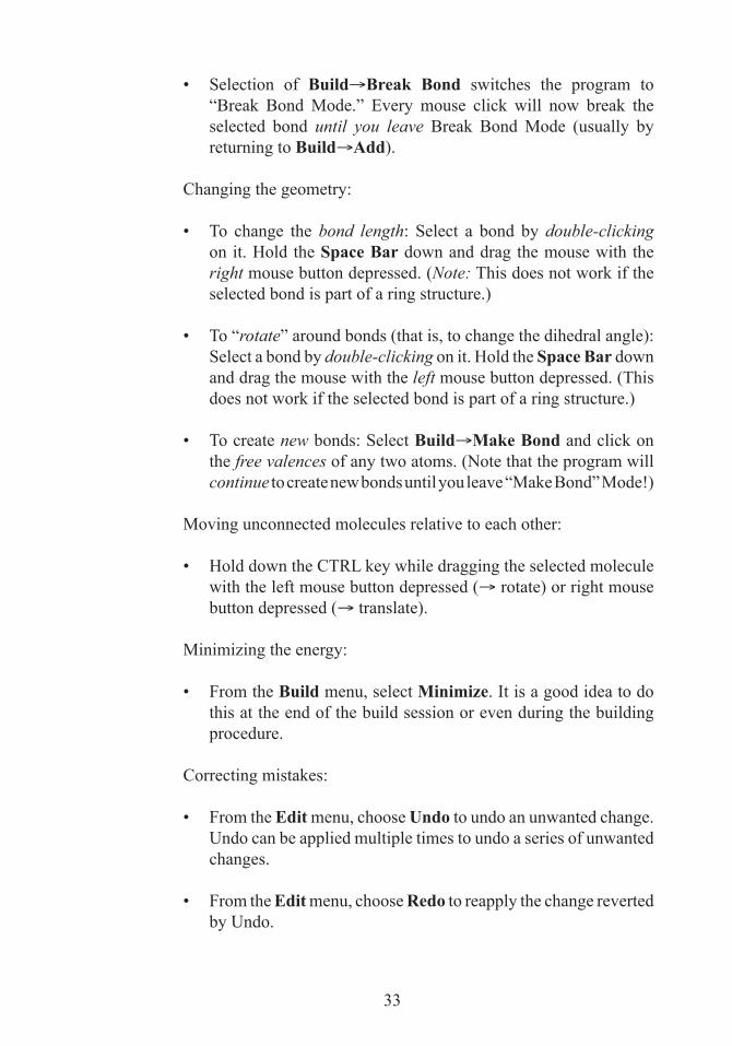
• Selection of Build→Break Bond switches the program to “Break Bond Mode.” Every mouse click will now break the selected bond until you leave Break Bond Mode (usually by returning to Build→Add).

Changing the geometry:

• To change the bond length: Select a bond by double-clicking on it. Hold the Space Bar down and drag the mouse with the right mouse button depressed. (Note: This does not work if the selected bond is part of a ring structure.)

• To “rotate” around bonds (that is, to change the dihedral angle): Select a bond by double-clicking on it. Hold the Space Bar down and drag the mouse with the left mouse button depressed. (This does not work if the selected bond is part of a ring structure.)

• To create new bonds: Select Build→Make Bond and click on the free valences of any two atoms. (Note that the program will continue to create new bonds until you leave “Make Bond” Mode!)

Moving unconnected molecules relative to each other:

• Hold down the CTRL key while dragging the selected molecule with the left mouse button depressed (→ rotate) or right mouse button depressed (→ translate).

Minimizing the energy:

• From the Build menu, select Minimize. It is a good idea to do this at the end of the build session or even during the building procedure.

Correcting mistakes:

• From the Edit menu, choose Undo to undo an unwanted change. Undo can be applied multiple times to undo a series of unwanted changes.

• From the Edit menu, choose Redo to reapply the change reverted by Undo.

34

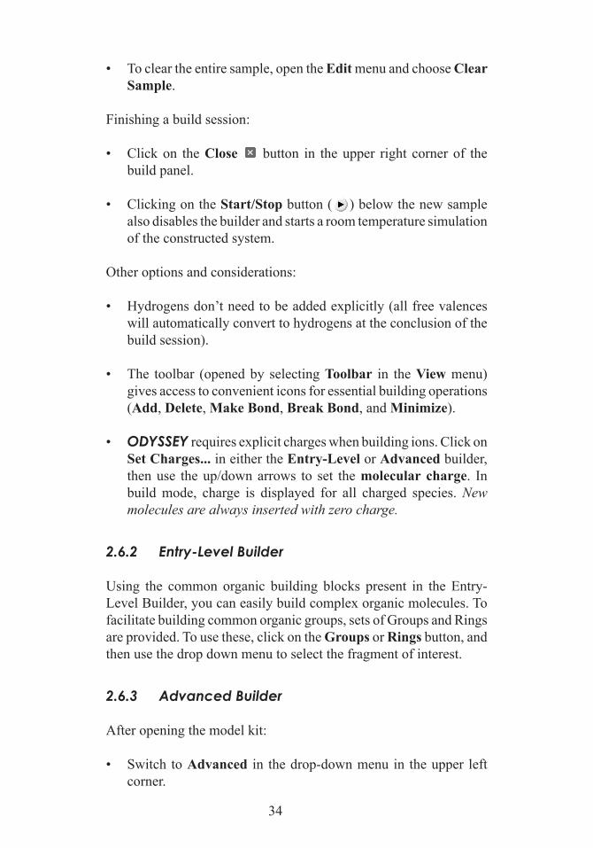
• To clear the entire sample, open the Edit menu and choose Clear Sample.

Finishing a build session:

• Click on the Close button in the upper right corner of the build panel.

• Clicking on the Start/Stop button ( ) below the new sample also disables the builder and starts a room temperature simulation of the constructed system.

Other options and considerations:

• Hydrogens don’t need to be added explicitly (all free valences will automatically convert to hydrogens at the conclusion of the build session).

• The toolbar (opened by selecting Toolbar in the View menu) gives access to convenient icons for essential building operations (Add, Delete, Make Bond, Break Bond, and Minimize).

• Odyssey requires explicit charges when building ions. Click on Set Charges... in either the Entry-Level or Advanced builder, then use the up/down arrows to set the molecular charge. In build mode, charge is displayed for all charged species. New molecules are always inserted with zero charge.

2.6.2 entry-Level Builder

Using the common organic building blocks present in the Entry-Level Builder, you can easily build complex organic molecules. To facilitate building common organic groups, sets of Groups and Rings are provided. To use these, click on the Groups or Rings button, and then use the drop down menu to select the fragment of interest.

2.6.3 advanced Builder

After opening the model kit:

• Switch to Advanced in the drop-down menu in the upper left corner.

35

• Select an Element from the drop-down periodic table (argon is the default).

• Select one of 12 different types of Coordination (the number and orientation of covalent bonds)

• To change the bond order: Select one of the four Bond Order icons, then double-click on any existing bond. (The second bond type is for “partial double” or aromatic bonds.)

• To declare non-zero charges of built molecules, click on Set Charges. In the subsequent dialog, use the up/down arrows to adjust the molecular charge for each molecule for which you need a non-zero charge.

Other options and considerations:

• The atom types can be changed at any time—simply select a new Element from the drop-down periodic table and double-click on the atom(s) to be changed. (This does not change the number of valences.)

• Building of coordination compounds is facilitated with special building blocks from the Ligands drop-down menu at the bottom of the build panel.

2.6.4 solid Builder

Odyssey’s molecular builder includes a number of prototypical solid structure types. After opening the model kit, switch to Solid (drop-down menu in the upper left corner).

• In the drop-down menu in the Solid panel, pick one of four crystal types: Ionic Solids, Metallic Solids, Molecular Solids, or Covalent Network Solids.

• Select one of the types in the list displayed. Click in the sample area to make the solid structure appear.

• You can change the number of replications of the basic cell with the Replication fields. (A reasonable default is provided

36

that is big enough to be interesting but small enough to simulate effectively.)

• For many of the solid types, you can also change the atom types and the charges. For example, there are several different solids that have the same structure as Sodium Chloride. (“Sodium Chloride Type” is available in the Ionic Solids section.) Both NaCl and CaO have this structure, but to build CaO, you would need to change Na to Ca and change Cl to O, then make sure that the charges are +2 and -2, respectively. For known structures the correct cell size is used, otherwise a rough estimate is used.

Note: 1) If the “start” button below the sample is faded out, the structure cannot be subjected to simulation. 2) The dimensions of the solid unit cell can be changed with the Solids tab of the Simulation Cell Builder.

2.6.5 peptide Builder

After opening the model kit, switch to Peptide in the drop-down menu in the upper left corner.

• There are three different options for building peptides: Single Amino Acid, α Helix, and β Sheet. You can choose between these using the radio buttons choices at the bottom of the peptide builder.

• For the Single Amino Acid selection, the chosen amino acid is displayed and can be inserted by clicking (or double-clicking for non-empty samples) on the background.

• For α Helix and β Sheet, clicking the amino acids adds them to the sequence panel. The amino acid sequence can be inserted by clicking (or double-clicking for non-empty samples) on the background. The sequence panel can be cleared by clicking the Clear button.

2.6.6 nucleotide Builder

After opening the model kit, switch to Nucleotide in the drop-down menu in the upper left corner.

37

• There are five different options for building nucleotides: Single Nucleotide (DNA), Single Nucleotide (RNA), DNA (Double Strand), DNA-RNA, and RNA (Single Strand). You can choose between these using the radio buttons at the bottom of the nucleotide builder.

• For the Single Nucleotide selections, the chosen nucleotide is displayed and can be inserted into an empty sample by clicking on the background. (You can only insert with the Nucleotide Builder into empty samples. To clear the sample, open the Edit menu and select Clear Sample.)

• For the three strand selections, clicking on the nucleotide adds them to the sequence panel. The sequence panel can be cleared with the Clear button. The nucleotide sequence can be inserted into an empty sample by clicking on the background.

2.6.7 Bulk sample Builder

To build bulk samples that are confined to containers with rigid walls (appropriate for gases):

• Use the molecule builder to build one molecule of each component of a mixture. (It does not matter how the molecules are spatially arranged.)

• From the Build menu, select Simulation Cell. By default, the molecule is in Vacuum at room temperature. (The Temperature can be explicitly declared in a textbox.)

• Switch to the Gas tab for building samples of gas. Declare the desired Temperature and Pressure in textboxes at the top of the cell build panel.

• Declare the desired number of molecules using the textbox that is labeled with the empirical formula of the molecule. For multicomponent mixtures, more than one textbox is present.

• The ratio of the simulation cell side lengths (aspect ratio) can be set at the bottom of the cell build panel (Cell Ratio). The default is for a cubic cell.

38

• Click on Apply to initiate the creation of the simulation cell. A progress bar will be displayed that indicates the progress of the build operation.

To build bulk samples that use periodic boundary conditions (appropriate for liquids and solutions):

• Start similarly to building gases, but switch to the Liquid tab after bringing up the Simulation Cell build panel. Declare the desired Temperature and Density at the top of the panel. Declare the desired number of molecules using the textbox(es) that is (are) labeled with the empirical formula(s) of the molecule(s).

• The ratio of the simulation cell side lengths can be set at the bottom of the cell build panel (Cell Ratio). The default is for a cubic cell.

• By default, periodic boundary conditions will be used for all three dimensions. Use the drop-down Periodic Boundary Conditions menu at the bottom of the panel to limit the periodicity to less than three dimensions; rigid walls will be used instead. (If you request rigid walls for all three dimensions, the resulting sample will have three rigid walls, like a gas sample.)

• Click on Apply to initiate the creation of the simulation cell. A progress bar will be displayed that indicates the progress of the build operation.

• If the simulation cell building step does not finish after a few minutes, then Abort and repeat with a set of “less challenging” system conditions.

To change the temperature and/or density of existing solid samples (retrieved from the stockroom or built with the Solid builder):

• Switch to the Solid tab after bringing up the Cell build panel.

2.6.8 adding Labels

Labels (as many as desired) can be attached to all samples:

• Select Build→New Label (or click on corresponding toolbar icon), then double-click on the background. Add any text.

39

• To edit an existing label, select Build→Edit a Label, double-click on the label and edit the text. Or right-click on the label and select Edit Label.

• To move an existing label, select the label and hold down the CTRL key while dragging the label with the right mouse button depressed.

• To delete a label, right-click on it and select Delete Label.

2.6.9 Changing Chirality While Building

Tetrahedral stereocenters of chiral molecules can be inverted by double-clicking on the stereocenter while holding down the CTRL key (Windows) or the key (Macintosh).

You can also invert stereocenters by right clicking: choose Invert Molecule Chirality (will invert all stereocenters simultaneously) or Invert Atom Chirality (will invert just the selected stereocenter).

2.6.10 energy Minimization

To minimize the energy of a sample:

• From the Build menu, select Minimize.

Systems with a boundary (typically gases, liquids, or solids) are minimized at constant volume.

For some samples, the energy minimizer and the dynamics option are deliberately disabled. If you really must minimize the energy of such a system, you can still do so after saving the sample as a new file.

2.6.11 name structure

To find the name of a molecule or system:

• From the Build menu, select Name.

If it can, Odyssey will report the name of the molecule(s). Molecules with more than 200 atoms cannot be named. For many

40

common molecules, Odyssey will display both the systematic name and the common name.

2.6.12 evaluate structure

Odyssey contains a facility to evaluate the chemical reasonableness of user-built or pre-built structures. To use this feature:

• From the Build menu, select Validity.

Odyssey will produce a list of questionable bonding centers, or will report that the model seems reasonable.

Note: Structures with more than 2,000 atoms cannot be evaluated.

2.7 preferences

2.7.1 setting the text size

The text size can be altered independent of the screen resolution:

• From the View menu, select Zoom Text→Zoom In (or →Zoom Out).

The program will remember your choice in future sessions.

2.7.2 physical Units

Odyssey uses the following default settings for property units in the Properties panel and in Plots:

Length: nm/pm

Temperature: °C

Pressure: atm

Energy: kJ/mol

41

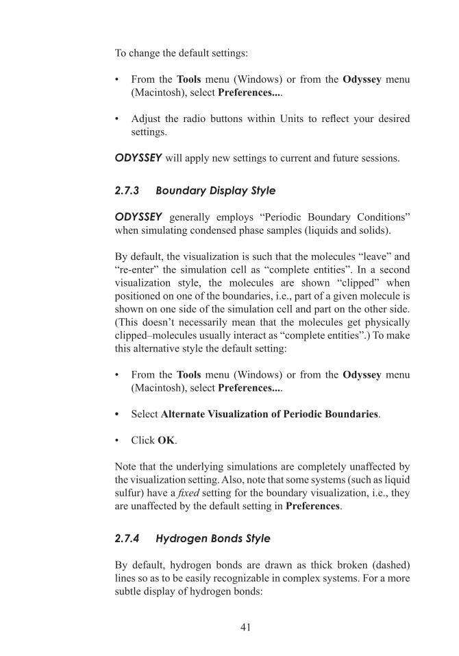
To change the default settings:

• From the Tools menu (Windows) or from the Odyssey menu (Macintosh), select Preferences....

• Adjust the radio buttons within Units to reflect your desired settings.

Odyssey will apply new settings to current and future sessions.

2.7.3 Boundary display style

Odyssey generally employs “Periodic Boundary Conditions” when simulating condensed phase samples (liquids and solids).

By default, the visualization is such that the molecules “leave” and “re-enter” the simulation cell as “complete entities”. In a second visualization style, the molecules are shown “clipped” when positioned on one of the boundaries, i.e., part of a given molecule is shown on one side of the simulation cell and part on the other side. (This doesn’t necessarily mean that the molecules get physically clipped–molecules usually interact as “complete entities”.) To make this alternative style the default setting:


• Select Alternate Visualization of Periodic Boundaries.

• Click OK.

Note that the underlying simulations are completely unaffected by the visualization setting. Also, note that some systems (such as liquid sulfur) have a fixed setting for the boundary visualization, i.e., they are unaffected by the default setting in Preferences.

2.7.4 Hydrogen Bonds style

By default, hydrogen bonds are drawn as thick broken (dashed) lines so as to be easily recognizable in complex systems. For a more subtle display of hydrogen bonds:

42


• Uncheck Emphasize Hydrogen Bonds.

• Click OK.

2.7.5 Color preferences

The default colors of the background and atom types can be set by the user:

• From the Edit menu, select Color. Select either the background or an atom of the desired chemical element.

• Adjust the mix of the three primary colors as desired (or click on Default for a reset).

• Close the dialog by clicking on .

Note that the color settings are global, i.e., they affect the display of all samples once the change has been made.

2.7.6 reduced Graphics for slower Machines

The graphical resolution sample can be set to lower quality whenever a given model is dynamically updated (either through mouse-induced rotation or via a physical simulation). This can help speed up the program when used with low performance graphics cards.

To change the graphics performance setting:


• Check (select) Reduced Graphics for Slower Machines.

• Click OK.

43

2.7.7 “expert” setting*

The “Expert” Setting is for Odyssey users that are familiar with the details of molecular dynamics simulations. If selected, the following queries are enabled by default:

Properties Panel:

• Potential Energy • Pressure

• Intermolecular Energy • PV/nRT (Compression Factor)

• Total Energy • Dihedral Angle

Plots:

• Radial Pair Distribution Function

“Expert” users are also able to save samples in the SMILES connectivity format for export to other programs.

To enable the “Expert” setting:


• Check (select) Expert.

• Click OK.

When in Expert mode, the Tools menu includes an Expert Keywords... option. It gives access to an input field where keywords for simulations can be set explicitly, such as:

• TIME_STEP=0.5 - use a fixed time step of 0.5 femtosec

• NVT - use an ensemble where the number of particles, the volume, and the temperature are held constant

• NVE - use an ensemble where the number of particles, the volume, and the energy are held constant

* Instructor’s Edition Only

44

• BOX - enclose the system in a container

• PBC - use periodic boundary conditions

• CUT_OFF=7.0 - evaluate electrostatic interactions up to a distance of 7.0 Angstrom

• SHAKE_BOND - constrain the bond lengths to their equilibrium values

• TEMP_MIN=100.0 - set the minimum allowed temperature to 100 K

• TEMP_MAX=1000.0 - set the minimum allowed temperature to 1000 K

• VOLUME_MIN=10.0 - set the maximum allowed volume to 10% of the initial volume

• VOLUME_MAX=500.0 - set the maximum allowed volume to 500% of the initial volume

Note: These and other keywords are only intended for true expert users, i.e., users who are intimately familiar with the technology of molecular-level simulations. Typical users of Odyssey will never need to declare or alter any keywords.

2.7.8 systematic and Common names

Molecules can be shown using their common names or their systematic (generally IUPAC) names. To change between the two, open the Preferences panel: From the Tools menu (Windows) or from the Odyssey menu (Macintosh), choose Preferences.... Then check or uncheck the “Use Systematic Names” option. Click the OK button to save your choice.

2.7.9 dipole Orientation

Samples with dipoles can either be displayed with the arrow pointing from positive to negative or from negative to positive (the latter is the IUPAC default). To change between these two settings, open the Preferences panel (from the Tools menu (Windows) or from the

45

Odyssey menu (Macintosh), choose Preferences...). Then check or uncheck the “Dipoles Negative to Positive (IUPAC)” option. Click the OK button to save your choice.

2.7.10 sound effects

The user can control whether a sound effect is generated whenever one of the Style→Collisions options is selected and two molecules collide.


• Check (or uncheck) Play Sounds.

2.8 Using Odyssey with Other programs, Files, and documents

2.8.1 reading pdB, XyZ, sMILes, Chemdraw, and IsIs/draw Files

Odyssey imports standard PDB files: (.pdb), XYZ files (.xyz), SMILES string files (.smi), ChemDraw files (.cdx), and ISIS/Draw files (.skc)

• Use the Open... dialog in the File menu.

2.8.2 Compatibility with Wavefunction’s spartan

Odyssey → spartan:

• Samples must be saved in the .spinput format before they can be opened with spartan. All atomic coordinates are fully recognized. However, “simulation cell-specific” information (such as the bounding box) is lost.

spartan → Odyssey:

• Files of type .spartan can be opened with Odyssey. Structural data and visualization features are fully recognized.

46

Minor differences in the display may exist; also note that Odyssey and spartan may use different default colors for many atom types.

• “Surface” data (Electron Densities, Potentials, Orbitals) can only be preserved in the Instructor’s Edition and then only by saving an entire lab in the .odylab format.

• If quantum mechanical calculations have been run on the file, Odyssey will use the calculated atomic charges (scaled so that each molecule has a whole number charge).

• For .spartan files that contain just one system, molecular dynamics will be available. For .spartan files with more than one system, molecular dynamics will not be available. Instead, a “Frameslider” will be present (see section 2.2.2 for information about Framesliders).

2.8.3 Using Odyssey with powerpoint

Odyssey can be seamlessly hyperlinked in PowerPoint presentations. You have the choice among the following possibilities:

• Hyperlinking individual samples (no accompanying text included)

• Hyperlinking experiments or stockroom pages

• Hyperlinking Odyssey’s home page.

The subsequent items provide corresponding instructions.

Note: When you run PowerPoint and use Odyssey hyperlinks, it is useful to open Odyssey beforehand (this makes the opening of simulations faster). It is not necessary to close Odyssey when moving from hyperlink to hyperlink since one copy of the program will be used for all of the linked simulations.

2.8.4 Hyperlinking Individual samples

• Save the sample that you want to hyperlink as an .xodydata file in a folder of your choice. Note that “surface” data such as

47

electron densities, potentials, and orbitals) will be lost (→ link through the initial page to access such samples).

• Creating the hyperlinks in PowerPoint:

• Windows: Use the “Hyperlink” attribute and navigate to the location of your saved .xodydata file.

• Macintosh: Use the “Action Settings” attribute (i.e., do not use the “Hyperlink” attribute). In the drop-down menu for “Hyperlink to”, select “Other File...” and navigate to the location of your saved .xodydata file.

• See Section 2.8.8 if you want to avoid the standard “security dialog” when opening hyperlinked .xodydata files.*

2.8.5 Hyperlinking Labs or stockroom pages/Windows*

Odyssey experiments (teaching units) can be hyperlinked into PowerPoint presentations. The following restriction applies:

• The hyperlink must refer to an ‘.odyssey’ file in its original location in the Odyssey folder. A copy of the file somewhere else will not do.

To create hyperlinks for Odyssey experiments, do the following:

• Find the ‘.odyssey’ file for your desired topic:

1. First find the Odyssey folder. In most cases, it is installed in the ‘Program Files→Wavefunction’ folder of ‘Local Disk (C:).’

For the teaching units, you will have to locate the correct .odyssey file for your desired topic by searching among the files in the “html” folder (the general organization is similar to that of an introductory chemistry textbook).

2. For stockroom models, you will have to find the correct .odyssey file in the “archive” folder. For example, the path for the ‘.odyssey’ file that is associated with “Liquid Water” is (depending on the version of the program) either:

* Windows Only

48

archive→Inorganic!Hydrogen Oxides.odyssey

or

archive→XCompounds!Water.odyssey

• See Section 2.8.8 if you want to avoid the standard “security dialog” when opening hyperlinked .odyssey files.

2.8.6 Hyperlinking Labs or stockroom pages/Macintosh*

To use PowerPoint hyperlinks to samples, labs, or stockroom pages, you need to go through the following steps once:

• Download the following file: “http://downloads.wavefun.com/MakeOdysseyHyperlinkFolder.sh”.

• Open a Terminal window.

• Type “sh ” (i.e., “sh” and a space)

• Drag MakeOdysseyHyperlinkFolder.sh into the terminal window.

• Drag Odyssey .app from its permanent location (usually the “Applications” folder) into the terminal window.

• Make sure that the terminal window is selected, then press the Return key.

The preceeding steps create a new alias Odyssey Hyperlinks side by side with the Odyssey application. In PowerPoint, you can now create hyperlinks for individual Odyssey files by using this alias:

• Whenever you wish to hyperlink an experiment or stockroom page (.odyssey), navigate through the Odyssey Hyperlinks alias to the desired file.

• If the Odyssey application is in its customary location in the “Applications” folder, you may have to manually edit each hyperlink path (in PowerPoint’s “Edit Hyperlink...” dialog) so as to start with file://localhost/Applications/...

* Macintosh Only

49

2.8.7 Hyperlinking the Home page

If you link to Odyssey’s initial page, you can access any lab and/or sample, via that hyperlink:

• In your PowerPoint slide, select the object that you wish to hyperlink.

• Right-click and select Action Settings.

• Select Run Program and browse for the name of the Odyssey executable:

• Windows: The executable in the Odyssey folder is either “OdysseyCollegeStudent.exe” (Student Edition) or “OdysseyCollegeInstructor.exe” (Instructor’s Edition) or an equivalent name for other versions of the program. In most cases, you will find the Odyssey folder in the “Program Files→Wavefunction” folder.

• Macintosh: The executable is either “Odyssey College X.X Student.app” (Student Edition) or “Odyssey College X.X Instructor.app” (Instructor’s Edition) or an equivalent name for other versions of the program. In most cases, you will find the file in the “Applications” folder.

Clicking on the object in the PowerPoint slide (when in presentation mode) will take you to the initial page of Odyssey. You can go wherever you wish from there.

2.8.8 suppressing the Windows security dialog*

To suppress the “Security Dialog” when hyperlinking into PowerPoint (all of the actions are required):

• Open PowerPoint.

• Select Tools→Options…

• Select Security tab.

* Windows Only

50

• Click on Macro Security…

• Select Low as the security setting.

• Click OK.

• Click OK.

• Close PowerPoint.

• Open any folder.

• Go to Tools→Folder Options…

• Select File Types tab.

• Scroll to and select the XODYDATA extension.

• Click on Advanced.

• Uncheck Confirm open after download.

• Click OK.

• Click OK.

• Close the open folder.

2.8.9 saving Odyssey pictures

Screenshots of samples can be saved in a variety of formats that allow for inclusion in other documents (Microsoft Word files, Web Pages, etc.):

• From the File menu, select Save Sample Image As....

• Choose a file name and one of the following file types:

.jpg (compressed) - Windows and Macintosh

.png (compressed, no loss) - Windows and Macintosh

51

.bmp (uncompressed) - Windows only

• Save the graphics file to the desired location.

Tip: For best resolution, zoom in prior to saving the screenshot. In the Instructor’s Edition, you can furthermore hide the text panel using the corresponding toolbar icon.

The clipboard (Edit→Copy Sample Image) can also be used to export pictures.

52

SCIENTIFIC BACKGROUND

3.1 Molecules in Motion: the Basic Idea Behind dynamic simulations

Odyssey’s simulations are very different from the simulations you may have encountered in other science media products. The motion of molecules does not arise because a human designer used a software tool to create an animation. Instead, Odyssey uses the basic laws of nature in order to represent molecular matter. The motion of molecules is an outcome of applying these laws, very much like the forces of gravity determine how the planets in the solar system move. In short, there is no “movie” file anywhere in Odyssey.

Suppose you want to simulate liquid water. When you load an Odyssey page with liquid water as the sample, you retrieve from a file the positions and velocities of water molecules in a simulation cell at an arbitrary moment in time. The following picture symbolizes the “start configuration”—for simplicity we represent water molecules as single spheres:

In order to perform a simulation, Odyssey must do several things:

1. Calculate the forces acting between the molecules—this is done using a set of rules that were developed by chemists and other scientists in years of laborious research. While partly empirical, the rules are based on a strict physical analysis of the forces that act between atoms.

The arrows in the following picture represent the computer’s knowledge of the forces acting on the molecules:

53

2. Next, Odyssey applies a formula that has been known since 1686! Newton’s Second Law states that the force acting on an object and the object’s acceleration are proportional:

F = m • a

Since we already know the force acting on a given water molecule (see above) and since the mass of a water molecule is well-known, we can now calculate the molecule’s acceleration. Knowing the molecule’s acceleration, however, amounts to being able to predict where it will move to and what its new velocity will be! More formally, this is called solving the “equations of motion,” and it is really no different than predicting the trajectory and velocity of a satellite that is fired off into space (all we need to know are the “initial conditions”).

If we apply this procedure to all water molecules in the simulation cell (in fact, it is applied to all molecules at once), we get the next snapshot of our system, or the next “time step”:

Molecular dynamics. In order to sustain a full-fledged simulation, all that is required is to repeat the same steps, again...and again…and again:

54

When you watch a simulation of liquid water in Odyssey, the computer is calculating “time steps”. (The program actually makes several steps between screen updates.) The steps are separated by approximately 10-15 sec of physical time—a very short time indeed! Typically, the computer calculates several thousand time steps during a simulation (up to hundreds of thousands of steps for some systems).

In the “start configuration” as well as at any time thereafter, each molecule has not only a position, but also a certain velocity. In fact, where the molecule will move to in the next step is affected by both the force acting on the molecule and its velocity. The molecule’s velocity is updated step after step, just like its position.

3.2 Calculation of Molecular Interactions

For each sample, Odyssey calculates the energy of interaction between the atoms that are present, regardless of whether the sample is an isolated molecule or a bulk phase with many molecules. The “potential function” is very complicated–there are many hundreds of parameters for the elements and valence states encountered in chemical compounds. At least conceptually, however, the potential function can be thought of containing the following main terms:

• Intermolecular attractive energy: an energy term that represents van der Waals forces (dispersion forces) between non-bonded atoms.

• Intermolecular repulsive energy: a steeply repulsive energy term for steric interactions at short distance that makes a close “overlap” of non-bonded atoms very unlikely.

• Coulomb energy (both inter- and intramolecular): energy term due to the assignment of “effective charges” to all the atoms of a molecule; at the intermolecular level, this energy represents charge-charge, charge-dipole, and dipole-dipole interactions.

repulsion

attraction

r

+

–

–

–

+

+

55

• Repulsive interactions between the molecules of the system and the confining walls (if there are any).

• Intramolecular energy of bond-stretching: the spring-like energy that it takes to distort a bond from its equilibrium bond distance. Note: This energy term (and sometimes also the following one) does not vary over time if Odyssey keeps the molecular geometry rigid.

• Intramolecular energy of angle-bending: the energy that it takes to distort any three bonded atoms from their preferred bond angle.

• Intramolecular energy of rotation around dihedral angles: a periodic function that describes the relative energies of the var ious “staggered” and “eclipsed” conformations of any four consecutively bonded atoms.

There are other terms, but essentially, it is the sum of these energies that yields the total energy of a given system. Calculation of the derivatives of the total energy with respect to the coordinates of all atoms yields the intermolecular forces that are at the heart of the algorithm that takes the system from one time step to the next (→Chapter 3.1). As the energy depends on the coordinates of all atoms in the system, the calculation must be repeated even when only a single atom moves.

• • • • •

•••

••

56

3.3 Why do Molecules of Liquids sometimes disappear?

When you carry out a simulation of a gas in Odyssey, you see molecules moving inside a container. That impression is perfectly appropriate: The molecules are confined by rigid “walls” from which they bounce off again and again as the simulation evolves.

However, when you carry out a simulation of a liquid the situation is somewhat different. You may notice that some molecules or atoms seem to leave the simulation cell, i.e., when close to one of the boundaries they often seem to be “gone” a few moments later. If you look carefully you will also notice the opposite, namely “new” molecules or atoms that seem to enter the simulation cell. Superficially, this coming and going is often perceived as a slight “flicker” at the simulation cell boundaries.

Why does this happen? The answer is that there really aren’t any “boundaries” when Odyssey simulates a liquid or solid—despite the obvious presence of a simulation cell! The trick is called periodic boundary conditions, and it is the approach which allows us to simulate true bulk matter (i.e., not a few molecules of liquid water, but the substance you get from the tap) even when we only have a very small simulation cell to work with.

Essentially, the simulation cell “wraps around” in each of the three dimensions. An easy way to visualize this wrapping around is to imagine that our simulation cell is surrounded by a set of identical replicas:

If a molecule in the center cell moves, then all its “copies” in the replica cells move at the same time—a perfectly coordinated motion.

57

Focus on the highlighted molecule. If the molecule “leaves” the central simulation cell towards the right, the molecule’s replica enters at the same time from the left. In effect, we have allowed the molecule to cross the system boundary while not losing anything—the system density remains perfectly constant.

The huge advantage of this approach is that there are no walls in the system that can interfere with the calculated bulk properties. Just think of a glass of water: The vast majority of the ~1023 molecules in the glass are not close to any of the container walls. Periodic boundary conditions allow us to accomplish the same in a simulation. In effect, the cell boundaries become a device for organizing the simulation rather than a representation of an actual container.

3.4 rigid Molecules and the speed of simulations

If you monitor the intramolecular bond distances during an Odyssey simulation, you may notice that often they do not change. Why? Keeping the molecules partially rigid is a common device for “speeding up” the simulations; it allows for using a larger physical time step than would otherwise be possible.

The rigidity is an excellent approximation of the real physical situation for very stiff hydrogen-containing bonds. More generally, it is of relatively little consequence for many calculated properties.

3.5 do the Calculated properties reproduce experimental data?

In many cases, there is qualitative agreement between calculated and experimentally measured properties. Particularly “trends” (such as variation with atomic mass, variation with dipole moment, or variation with temperature) are often predicted correctly. Predictions that are quantitatively correct are rare as the program employs models that are computationally inexpensive and therefore imperfect.

While not very common, outright failures also occur. However, it should be kept in mind that the presence of failures and limitations is a defining characteristic of all models—not only scientific models, but also models anywhere else. The pedagogical value of models

58

derives from their ability to be experimented with, not from being perfect replacements of the “real thing.”

3.6 does Odyssey assume Ideal Gas Behavior?

Odyssey never assumes ideal gas behavior. Gas molecules are always modeled as particles of finite volume that exhibit non-negligible interactions (if sufficiently close).

Nevertheless, ideal gas behavior will be observed in many situations, namely whenever the physical conditions happen to closely correspond to the assumptions that are implicit in the Ideal Gas Law.

3.7 Gravity in Odyssey

You may have noticed that if you turn a partially filled simulation cell “upside down”, the liquid doesn’t flow to the bottom. The reason for this at first glance strange behavior is not the omission of the Earth’s gravitational field (it is easy to include), but the fact that gravitational forces are so weak that they do not make a difference on the time scale of molecular simulations. Much longer simulations (and macroscopic sample sizes) would be needed to observe gravity-driven flow.

Incidentally, even macroscopic samples can behave the way molecular samples behave in Odyssey. All that is needed is an environment where the effects of gravity are not noticeable–as is the case for any orbiting spacecraft. One could well say that Odyssey conveys an idea of what handling substances on the International Space Station would feel like!

A familiar phenomenon that crucially depends on the presence of gravitational forces is the formation of “neat” interfaces. In Odyssey, you will in fact find models of immiscible liquids that show fairly straight interfaces, but this is only because they have been set up to show the “expected” pattern.

59

3.8 Condensing Gases

Given sufficient simulation time and a sufficiently low temperature, samples of gas will eventually show condensation. However, the condensation will happen via the formation of irregular molecular clusters rather than through the formation of a “neat” horizontal interface. The reason for this is the insignificance of gravitational forces on the time scale of molecular simulations.

3.9 Liquids Won’t Freeze

Odyssey focuses on real simulations of physical phenomena, rather than on cartoon-style animations. While the freezing transition can be simulated, it is very hard to do and requires sample sizes and time scales that lie beyond the scope of Odyssey.

3.10 density doesn’t Change When Melting

Odyssey performs its simulations with unit cells of constant volume. The user has to manually adjust the volume in order to represent changes in density:

• From the View menu, select Properties....

• From the Add Property menu, select first System → Density and then Thermodynamics → Volume.

• Adjust the volume with the provided slider so as to reach the desired density.

Alternatively, the Build → Simulation Cell → Liquid tab can be used for density adjustments.

3.11 Molecules don’t dissociate

Although Odyssey is capable of simulating the breaking and forming of covalent bonds, such systems require careful preparation and a thorough description of the reaction. Odyssey itself is not

60

capable of deducing possible reactions. Unless the system has been set up beforehand to include reactions, chemical change with breaking of covalent bonds cannot happen.

3.12 Ions don’t dissolve across an Interface

While Odyssey is capable of representing a large variety of physical and chemical processes, the program cannot directly carry out real-time simulations when the time scale of the process in question does not fit within the typical picosecond (10–12 sec) time range that is accessible to the program.

The process of dissolving an ionic solid falls into this category. In principle, ions may well break away from the solid, but the process is an extremely “rare event” and in practice will not be observed.

3.13IdentificationofHydrogen Bonds

ODYSSEY identifies a hydrogen bond when an atom with an attached hydrogen is close to another atom and all of the following criteria are satisfied:

• The partnering atoms must involve a known hydrogen bond donor and a known hydrogen bond acceptor. Oxygen, nitrogen, and fluorine are the most important formers of hydrogen bonds, but not necessarily in all valence states. In liquid water, for example, sp3 oxygen acts as both a donor and an acceptor of hydrogen bonds. The sp2 oxygen of carbonyl groups, on the other hand, can only act as an acceptor and must pair up with some other donor if it is to form a hydrogen bond.

• The distance between the hydrogen atom and the acceptor atom must fall within a range of 122-260 pm.

• Overtly bent hydrogen bonds are excluded by requiring that the angle ∠ (hydrogen atom-donor atom-acceptor atom) is smaller than a set value. For example, for oxygen and nitrogen this angle is 30°.

61

3.14 Calculation of enthalpies, entropies, and Free energies

For select compounds under a certain set of conditions (temperature, pressure, and phase), ODYSSEY calculates several thermodynamic functions:

Enthalpy:

In order to allow for an intuitive interpretation of the thermodynamic consequences of temperature and phase changes, ODYSSEY adopts a unique reference state for enthalpies. The displayed values (from empirical formulas that represent best fits of experimental data) are always relative to the elements in their standard states at 25°C. Note that this is different from what is implicit in many thermodynamic tables:

• If thermodynamic tables give standards heats of formation as a function of temperature, the assumed reference state is temperature dependent (because the enthalpy of formation of the stable phase of an element is by definition zero for all temperatures).

• If thermodynamic tables give (H°-H°298) data, then the implied reference state changes from phase to phase and from substance to substance.

ODYSSEY refrains from working with varying reference states.

Entropy:

ODYSSEY displays standard entropies. The algorithm used depends on the complexity of the given system and involves combinations of analytical statistical thermodynamic theory and empirical formulas (with the latter representing best fits of experimental data).

Free Energy:

In order to allow for an intuitive interpretation of the thermodynamic consequences of temperature and phase changes, ODYSSEY adopts a unique reference state for free energies. The displayed values (calculated from the underlying enthalpy and entropy data) are always

62

relative to the elements in their standard states at 25°C. Note that this is different from what is implicit in many thermodynamic tables:

• If thermodynamic tables give standard free energies as a function of temperature, the assumed reference state is temperature dependent (because the free energy of the stable phase of an element is by definition zero for all temperatures).

• If thermodynamic tables give (G° - G°298) data, then the implied reference state changes from phase to phase and from substance to substance.

ODYSSEY refrains from working with varying reference states.

63

TEACHING USAGE

4.1 simulating the Liquid-Vapor transition

The liquid-vapor transition can easily be simulated for many systems:

• Retrieve a sample of liquid from the Molecular Stockroom, or build one yourself using the Model Kit (you will need to know the density of the desired liquid).

• From the View menu, select Properties....

• From the Add Property menu, select first Thermodynamics → Temperature and then Thermodynamics → Volume.

• Start the simulation.

• Overwrite the Volume Field by a number that is at least 100 times bigger than the number shown.

• Resize the view of the simulation cell: Edit → Resize.

• To speed up the process of evaporation, click on “Temperature” and increase its value with the slider provided.

4.2 Incorporating simulations into presentations and Classwork

To incorporate Odyssey simulations into lectures, laboratory experiments, and homework assignments:

• Make the corresponding molecular sample (normally an .xodydata file) available on a computer that has Odyssey installed.

• Run the corresponding simulation live and use the visualization and system manipulation features of the Odyssey interface.

64

See Section 2.8.3 for help on linking Odyssey simulations directly in PowerPoint.

Note: Since Odyssey is organized around the paradigm of live, interactive simulations, corresponding “movies” cannot be saved.

4.3 Can Odyssey Be Used with Interactive Whiteboards?

Odyssey is well suited for classrooms that are equipped with Smartboards or other interactive whiteboards.

4.4 annotating pages

All Odyssey pages can be individually annotated:

• Click on the “document” icon (looks like a piece of notebook paper) at the top of the text panel. This opens a Notes page that accepts any text that is entered.

• Return to the originating page by clicking on the SAVE+CLOSE link at the bottom of the Notes page.

The annotations for a given Experiment or Stockroom entry are retained by the computer and will be shown whenever you return to the corresponding Notes page later.

65

COMPUTER QUESTIONS AND TROUBLESHOOTING

5.1 Graphics performance

If the graphics performance is unsatisfactory when using the “Space-Filling” style:

• In the Tools menu (Windows) or Odyssey menu (Macintosh), select Preferences.

• Check Reduced Graphics for Slower Machines. Click OK.

5.2 running on Battery

If the graphics performance is unsatisfactory when running on battery:

• In the Tools menu (Windows) or Odyssey menu (Macintosh), select Preferences.

• Check Reduced Graphics for Slower Machines. Click OK.

On some computers, you may notice a certain “jumpiness” of the simulations while running on battery. This is due to repeated and automatic cycling of the processor between different clock speeds. Changing the power management setting of your machine to “Presentation” is likely to remedy this problem.

5.3 Graphics Hardware acceleration*

Try to lower the “Graphics Hardware Acceleration” if Odyssey crashes immediately after installation:

• Go to Start Menu→Settings→Control Panel→Display→ Settings→Advanced→Troubleshoot.

* Windows only

66

• Set the “Hardware Acceleration Slider” to the highest setting that still allows the program to run properly.

5.4 Windows Operating system requirements

Odyssey requires Windows 7, Windows Vista, or Windows XP. The program will not run under Windows 98 or Windows ME.

5.5 Macintosh Operating system requirements

Odyssey requires Mac OS X 10.7 Lion, Mac OS X 10.6 Snow Leopard, or Mac OS X 10.5 Leopard. Only Intel chips are supported.

5.6 differences Between pre-Built and User-Built samples

When building molecules and bulk phase samples from scratch, Odyssey draws on a set of all-purpose rules and parameters (since the structure space of chemistry is huge and the computer obviously doesn’t exactly know what you are after). Pre-built samples in Odyssey, on the other hand, are often defined with custom settings that help with improving the general quality of the model.

As a consequence, user-built samples will occasionally not “behave as well” as the pre-built samples. However, it is rare for a user-built sample to behave completely differently.

5.7 problems with Collision or Velocity Highlighting

The “Collisions” and “Velocities” attributes (in the Style menu) are only available for samples whose density is not too high (this protects the computer from problems such as being overwhelmed by collision counting in higher density samples). A rule of thumb is that letting the pressure drop to less than ~10 atm (use Build → Simulation Cell → Gas) will make the attributes available.

67

5.8 Vapor Molecules don’t seem to Move Fast enough

When comparing gases with liquids or solids, the molecular motion in the former often appears to be “slow” rather than fast. Why is that?

In order to facilitate observations of a wide variety of systems, Odyssey autoscales the size of the simulation cell to the screen size regardless of the physical state of the substance. As gas phase simulation cells are typically much bigger than condensed phase simulation cells (compare the “1 nanometer lines” in the corners of the simulation cells), the net motion in the gas phase is in fact much faster than the net motion in the liquid phase.

5.9 Creating File associations*

Before you can hyperlink an Odyssey file into a PowerPoint presentation, you may have to register the .xodydata file extension with the Windows operating system (in this way PowerPoint will know that it needs to start Odyssey when encountering hyperlinks to .xodydata files):

1. Try to directly open the .xodydata file by double clicking on its icon. If Odyssey starts up and the model displays, you don’t need to do anything else.

2. If Odyssey doesn’t start up, right-click on the .xodydata file and select Open With…, and then select Choose Program. In the resulting dialog, navigate to the Odyssey folder and select “OdysseyCollegeStudent.exe” (Student Edition) or a similarly named executable for other versions of the program. In most cases, you will find the Odyssey folder in the ‘Program Files→Wavefunction’ folder of ‘Local Disk (C:)’. Check the “Always Open With This Program” option (this creates a registry entry).

3. Open the file, then close Odyssey.

* Windows only

68

Any file of the type .xodydata can now be hyperlinked into PowerPoint slides via the ‘Hyperlink’ attribute. All features of the Odyssey interface (simulation control icons, etc.) are fully available.

5.10 suppressing the “Blocked Content” Message Bar when printing pdF-Formatted Worksheets*

• Open Internet Explorer.

• Select Tools → Internet Options....

• Select Advanced tab.

• Scroll to Security section.

• Check Allow active content to run in files on My Computer.

• Close Internet Explorer.

5.11 Opening saved Models with “drag and drop”

All Odyssey files (.xodydata or .odyssey) and also all .spartan files can be opened by dragging the file onto the desktop shortcut created by the installer.

5.12 Importing From Other Modeling programs

Odyssey reads .pdb files (generated by most other modeling programs and also the file format of many databases) as well as .spartan files (generated by Wavefunction’s program spartan). In addition, it reads ChemDraw, ISIS/Draw, XYZ and SMILES files. Use File → Open in order to import an external file or use “Drag and Drop”.

* Windows only

69

5.13 Uninstalling the Windows Version

To uninstall the Windows version of Odyssey:

• Use the Uninstall shortcut in the Odyssey program group that is found in Start → All Programs.

If the Uninstall shortcut in the Odyssey program group is not available:

• Use the Start Menu → Control Panel → Add or Remove Programs dialog.

70

A

Abort Simulation Cell Building ..38Activation ..............................2,4,73Adding Labels .............................38Adding Molecules ..................32,34Adding Plots................................26Advanced Builder .......................34α-Helix ........................................36Alternate Visualization ................41Amino Acid Sequence .................36Angle-Bending ............................55Animations .............................13,52Annotating ..............................10,64Answer Key ...........................18,19Area Select ..................................18Aspect Ratio ................................37Atom Color .................................42Attractive Energy ........................54Averaged Values ..........................25

B

Background Color .......................42Ball and Spoke Style ..............17,18Ball and Wire Style .....................17Bar-Style (Histograms) ...............31Battery .........................................65β-Sheet ........................................36Binding Energy ...........................21Bins (Histograms) .......................32Blocked Content ..........................68BMP Files ..............................16,51Bond Length Changes .................33Bond Order ..................................35

INDEX

Bond-Stretching ..........................55Boundary Conditions ........38,41,56Boundary Display Style ..............41Breaking Bonds ......................33,34Building.......................................32Build Menu .............32,33,37,38,39Bulk Sample Builder ..............36,37

C

Cell Builder .......................36,37,38Cell Ratio ...............................37,38Centering .....................................23Changing Atomic Charges ..........36Changing Composition ...............26Changing Molecular Charges......34Changing Slider Limits ...............26Changing System Parameters .....25Changing Temperature ................25Changing the Geometry ..............33Changing the Number of Molecules ....................................26Changing Volume ........................25Charge Labels .............................21ChemDraw .............................45,68Chirality .................................14,39Clearing Plots ..............................27Clipping Feature ..........................20Clipping Sphere Radius ..............21Collisions ...............................19,66Color by Property ...................21,22Common Names .......................4,44Comparing Samples ....................23Compatibility with spartan .....45

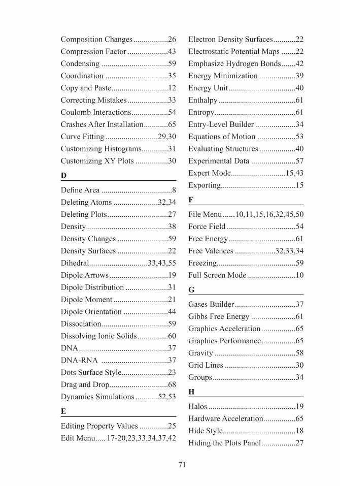
71

Composition Changes .................26Compression Factor ....................43Condensing .................................59Coordination ...............................35Copy and Paste ............................12Correcting Mistakes ....................33Coulomb Interactions ..................54Crashes After Installation ............65Curve Fitting ..........................29,30Customizing Histograms .............31Customizing XY Plots ................30

D

Define Area ...................................8Deleting Atoms ......................32,34Deleting Plots ..............................27Density ........................................38Density Changes .........................59Density Surfaces .........................22Dihedral .............................33,43,55Dipole Arrows .............................19Dipole Distribution .....................31Dipole Moment ...........................21Dipole Orientation ......................44Dissociation .................................59Dissolving Ionic Solids ...............60DNA ............................................37DNA-RNA .................................37Dots Surface Style .......................23Drag and Drop .............................68Dynamics Simulations ...........52,53

E

Editing Property Values ..............25Edit Menu ..... 17-20,23,33,34,37,42

Electron Density Surfaces ...........22Electrostatic Potential Maps .......22Emphasize Hydrogen Bonds .......42Energy Minimization ..................39Energy Unit .................................40Enthalpy ......................................61Entropy ........................................61Entry-Level Builder ....................34Equations of Motion ...................53Evaluating Structures ..................40Experimental Data ......................57Expert Mode ...........................15,43Exporting .....................................15

F

File Menu ......10,11,15,16,32,45,50Force Field ..................................54Free Energy .................................61Free Valences ....................32,33,34Freezing .......................................59Full Screen Mode ........................10

G

Gases Builder ..............................37Gibbs Free Energy ......................61Graphics Acceleration .................65Graphics Performance .................65Gravity ........................................58Grid Lines ...................................30Groups .........................................34

H

Halos ...........................................19Hardware Acceleration ................65Hide Style ....................................18Hiding the Plots Panel .................27

72

Hiding the Properties Panel ........25Hiding the Text Panel ....................9Histograms ..................................30Hydrogen Bonds ....................19,60Hydrogen Bonds Style ................41Hyperlinking ...........46,47,48,49,67

I

Icons ..............................................5Ideal Gas Behavior ......................58Importing ................................45,68Instantaneous Values ...................25Instructor Comments ...................12Interactive Whiteboards ..............64Ionic Solids .................................35ISIS/Draw ...................................68IUPAC Names ..........................4,44

J

JPG Files ................................16,50

K

Keywords ....................................43

L

Labels for Plot Axes ...............30,32Length Unit .................................40Ligands Menu .............................35Linear Fit ................................29,30Line Style (Histograms) ..............31Liquids Builder ...........................38Liquid-Vapor Transition ..............63Lone Pairs ...................................19

M

Making Bonds ........................33,34Measuring Properties ..................24

Melting ........................................59Mesh Surface Style .....................23Metallic Solids ............................35Minimization .....................33,34,39Molecular Charge ........................34Molecular DynamicsSimulations .......................13,52,53Molecular Interactions ................54Molecular Labs .......................2,3,7Molecular Solids .........................35Molecular Stockroom .........2,4,7,16Molecular Trails ..........................20Molecule-Molecule Collisions ....19Molecule-Wall Collisions ...........19Mouse Functions ...........................7Movies....................................52,64Moving a Selected Molecule .14,33Moving Labels ............................39Moving the Plot Legend ..............30

N

Naming Structures ......................39Newton’s Law .............................53Notes ......................................10,64Nucleotide Builder .................22,36Number of Molecule Changes ....26

OOctahedral Stereocenters ............15Odyssey Menu ...................... 41-45Operating System Requirements .66

P

Pair Distribution Function...........43Parameter Plots ...........................29PDB Files ...............................45,68

73

Peptide Builder .......................22,36Periodic BoundaryConditions .........................38,41,56Periodic Table .............................11Physical Properties ......................24Physical Units .............................40Pictures of Models ......................50Plot Legend .................................30Plots.........................10,12,26,31,43PNG Files ...............................16,50Point-to-Point .........................29,30Potential Energy ..........................43PowerPoint ...................46,48,49,64Preferences ............... 4,12,40-45,65Presentation Mode ........................9Pressure ..................................37,43Pressure Unit ...............................40Printing ........................................10Print Preview ...............................10Projector Friendly Colors ..............9Properties ....................................24Properties as a Color Value ....21,22Properties Panel ..........................43Properties Table ...........................11

R

Radial Pair Distribution Function ......................................43Radio Buttons............3,14,36,37,41Range of Plots ........................30,32Reactions ................................20,60Reactive Events ...........................20Recording of Data Points ............29Redo ............................................33Reduced Graphics ..................42,65

Refresh ..........................................9Replications .................................35Resizing .......................................23Ribbons .......................................22Rigid Geometry ......................55,57Rings ...........................................34RNA ............................................37Rotating Around Bonds............8,33

S

Samples Setting (Histograms) .....31Saving Samples ...........................15Scatter Plot .............................29,30Screen Layout ...............................5Screenshots ............................12,16Scroll Wheel ..........................2,7,21Select Atom/Molecule/Group/All.................................17,18,19,20,24Sequences of Frames ...................13Set Clipping Center .....................21Show Comments by Default .......12Single Amino Acid ......................36Single Nucleotide ........................37Slider ......................................14,25Smartboards ................................64SMILES ............................15,45,68Smoothed Fit ..........................29,30Solid Builder ...............................35Solid Surface Style ......................23Space Filling Style ......................17Speed Distribution ......................31Speeds .........................................20spinput ....................................15,45Starting Simulations ...............13,34Status Bar ......................................9

74

Step Forward .................................5Step Reverse ..................................5Stereocenters .....................14,15,39Stopping Simulations .............13,34Styles ...........................................16Surfaces .......................................22Switching Samples ......................14Synchronizing Simulations .........24

T

Tabs ............................................4,7Temperature ...........................37,38Temperature Changes ..................25Temperature Unit ........................40Tetrahedral Stereocenters ............14Text Panel .................................9,11Text Size ......................................40Time Plots ...................................30Time Step ..........................13,43,54Title of Plots ...........................30,31Toolbar .....................................6,34Tools Menu .............. 4,11,12,41-45Total Energy ................................43Trails ...........................................20Trajectories ..................................20Translational Kinetic Energy ......21Translational Kinetic EnergyDistribution .................................31Transparent Surface Style ...........23Troubleshooting ..........................65Tube Style ..............................17,18

U

Undo ............................................33Uninstalling .................................69

Units ............................................40

V

Vacuum Conditions .....................37van der Waals Forces ..................54Velocities ................................20,66View Menu ........6,7,10,24,26,31,34Volume Changes .........................25

W

Walls.............................37,55,56,57Webpage-Style Controls ...............3Windows Security Dialog ...........49Wire Style ...................................17

X

XY Plots ......................................27XY Plots with a Parameter ..........29XYZ Files...............................45,68

Y

Yellow Spokes .............................32

Z

Zoom .....................................7,8,21

Zoom Text ...................................39