Use Predictor Corrector Scheme - ECMWF

357

On the use of apredictor-corrector scheme tocouple the dynamics with the

physical parametrizations in theECMWF model

M. J. P. Cullen and D. J. Salmond

Research Department

Submitted for publication in Q. J. Roy. Met. Soc.

January 2002

For additional copies please contact

The LibraryECMWFShinfield ParkReadingRG2 [email protected]

Series: ECMWF Technical Memoranda

A full list of ECMWF Publications can be found on our web site under:http://www.ecmwf.int/pressroom/publications/

c©Copyright 2002

European Centre for Medium Range Weather ForecastsShinfield Park, Reading, RG2 9AX, England

Literary and scientific copyrights belong to ECMWF and are reserved in all countries. This publicationis not to be reprinted or translated in whole or in part without the written permission of the Director.Appropriate non-commercial use will normally be granted under the condition that reference is madeto ECMWF.

The information within this publication is given in good faith and considered to be true, but ECMWFaccepts no liability for error, omission and for loss or damage arising from its use.

http://www.ecmwf.int/pressroom/publications/

On the use of a predictor-corrector scheme to couple the dynamics with the physical parametrizations . . .

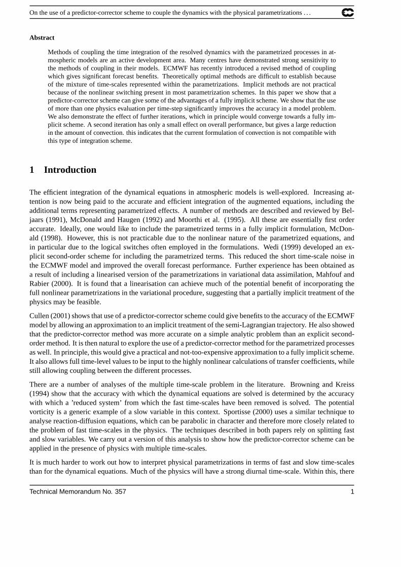
Abstract

Methods of coupling the time integration of the resolved dynamics with the parametrized processes in at-mospheric models are an active development area. Many centres have demonstrated strong sensitivity tothe methods of coupling in their models. ECMWF has recently introduced a revised method of couplingwhich gives significant forecast benefits. Theoretically optimal methods are difficult to establish becauseof the mixture of time-scales represented within the parametrizations. Implicit methods are not practicalbecause of the nonlinear switching present in most parametrization schemes. In this paper we show that apredictor-corrector scheme can give some of the advantages of a fully implicit scheme. We show that the useof more than one physics evaluation per time-step significantly improves the accuracy in a model problem.We also demonstrate the effect of further iterations, which in principle would converge towards a fully im-plicit scheme. A second iteration has only a small effect on overall performance, but gives a large reductionin the amount of convection. this indicates that the current formulation of convection is not compatible withthis type of integration scheme.

1 Introduction

The efficient integration of the dynamical equations in atmospheric models is well-explored. Increasing at-tention is now being paid to the accurate and efficient integration of the augmented equations, including theadditional terms representing parametrized effects. A number of methods are described and reviewed by Bel-jaars (1991), McDonald and Haugen (1992) and Moorthi et al. (1995). All these are essentially first orderaccurate. Ideally, one would like to include the parametrized terms in a fully implicit formulation, McDon-ald (1998). However, this is not practicable due to the nonlinear nature of the parametrized equations, andin particular due to the logical switches often employed in the formulations. Wedi (1999) developed an ex-plicit second-order scheme for including the parametrized terms. This reduced the short time-scale noise inthe ECMWF model and improved the overall forecast performance. Further experience has been obtained asa result of including a linearised version of the parametrizations in variational data assimilation, Mahfouf andRabier (2000). It is found that a linearisation can achieve much of the potential benefit of incorporating thefull nonlinear parametrizations in the variational procedure, suggesting that a partially implicit treatment of thephysics may be feasible.

Cullen (2001) shows that use of a predictor-corrector scheme could give benefits to the accuracy of the ECMWFmodel by allowing an approximation to an implicit treatment of the semi-Lagrangian trajectory. He also showedthat the predictor-corrector method was more accurate on a simple analytic problem than an explicit second-order method. It is then natural to explore the use of a predictor-corrector method for the parametrized processesas well. In principle, this would give a practical and not-too-expensive approximation to a fully implicit scheme.It also allows full time-level values to be input to the highly nonlinear calculations of transfer coefficients, whilestill allowing coupling between the different processes.

There are a number of analyses of the multiple time-scale problem in the literature. Browning and Kreiss(1994) show that the accuracy with which the dynamical equations are solved is determined by the accuracywith which a ’reduced system’ from which the fast time-scales have been removed is solved. The potentialvorticity is a generic example of a slow variable in this context. Sportisse (2000) uses a similar technique toanalyse reaction-diffusion equations, which can be parabolic in character and therefore more closely related tothe problem of fast time-scales in the physics. The techniques described in both papers rely on splitting fastand slow variables. We carry out a version of this analysis to show how the predictor-corrector scheme can beapplied in the presence of physics with multiple time-scales.

It is much harder to work out how to interpret physical parametrizations in terms of fast and slow time-scalesthan for the dynamical equations. Much of the physics will have a strong diurnal time-scale. Within this, there

Technical Memorandum No. 357 1


are much faster time-scales, such as those involved in the generation of precipitation. Some of the physicalprocesses will be strongly coupled to dynamical time-scales; for instance latent heat release will be closelycoupled to vertical motion. In the dynamical equations, the natural split is between the potential vorticitycontrolled dynamics as ’slow’ and the inertio-gravity waves as ’fast’. This can only be illustrative, as on somescales the inertio-gravity wave frequency is less then the diurnal frequency which is a main time-scale for thephysics. However, by making such a scale separation, we can clarify the options for time integration of thephysics.

We apply the predictor-corrector integration of the physics to the current version of the ECMWF model. Thismodel is part of the IFS (Integrated Forecasting System) developed jointly with Meteo-France. The currentimplementation at ECMWF uses the two-time-level semi-Lagrangian integration scheme, Temperton et al.(2001). Recent developments to the parametrizations are described by Gregory et al. (2000). We show howeach of the current parametrizations can be interfaced with the predictor-corrector scheme. However, we alsoshow that there could be advantages if there was more consistency between the formulations of the differentschemes.

2 Time Integration schemes for dynamics and parametrizations

2.1 Analysis of schemes with multiple time-scales

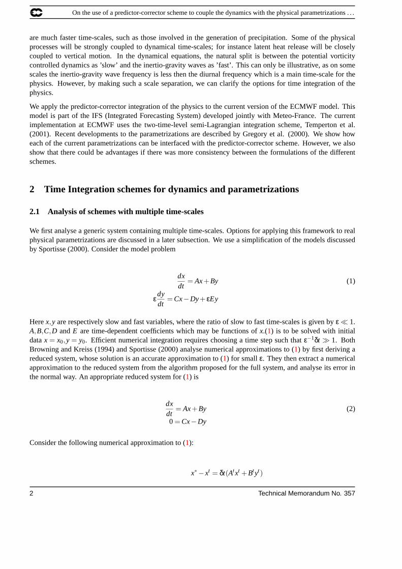
We first analyse a generic system containing multiple time-scales. Options for applying this framework to realphysical parametrizations are discussed in a later subsection. We use a simplification of the models discussedby Sportisse (2000). Consider the model problem

dxdt

= Ax+By (1)

εdydt

= Cx−Dy+ εEy

Herex,y are respectively slow and fast variables, where the ratio of slow to fast time-scales is given byε� 1.A,B,C,D andE are time-dependent coefficients which may be functions ofx.(1) is to be solved with initialdatax = x0,y = y0. Efficient numerical integration requires choosing a time step such thatε−1δt � 1. BothBrowning and Kreiss (1994) and Sportisse (2000) analyse numerical approximations to (1) by first deriving areduced system, whose solution is an accurate approximation to (1) for smallε. They then extract a numericalapproximation to the reduced system from the algorithm proposed for the full system, and analyse its error inthe normal way. An appropriate reduced system for (1) is

dxdt

= Ax+By (2)

0 = Cx−Dy

Consider the following numerical approximation to (1):

x∗−xt = δt(Atxt +Btyt)

2 Technical Memorandum No. 357


y∗−yt = ε−1δt(C∗x∗−D∗y∗+ εEtyt) (3)

xt+δt −xt =12

δt(Atxt +A∗x∗+Btyt +B∗y∗)

yt+δt −yt = ε−1δt(Ct+δtxt+δt −Dt+δtyt+δt + εE∗y∗

)This implies the following numerical approximation to the reduced system, eq. (2):

x∗−xt = δt(Atxt +Btyt)0 = C∗x∗−D∗y∗ (4)

xt+δt −xt =12

δt(Atxt +A∗x∗+Btyt +B∗y∗)

0 = Ct+δtxt+δt −Dt+δtyt+δt

Substituting fory in terms ofx, the final update ofx becomes

xt+δt −xt =12

δt(Atxt +A∗x∗+(BD−1C)txt +(BD−1C)∗x∗) (5)

We see that this is simply a predictor-corrector approximation to the evolution equation forx derived from (2),and is thus second order accurate. According to Sportisse (2000), we can therefore expect it to be second orderaccurate in practice for approximations to (1) with δt � ε.

2.2 Comparison of integration schemes for a problem with multiple time-scales

We illustrate with a simple example. The problem to be solved is

dxdt

= cos(t + .4y) (6)

dydt

= C(x−y(1+ .5sin(3x)))

Here,C is a constant chosen much greater than 1. The coefficients are chosen to introduce nonlinearity, but thecoefficients in the equation for the fast variable only depend on the slow variable. The reduced system for (6)replaces the second equation by the diagnostic relation

0 = x−y(1+ .5sin(3x)) (7)

We compare the following schemes:

i) Simple split

xt+δt −xt = δtcos(t + .4yt) (8)

yt+δt −yt = Cδt(xt+δt −yt+δt(1+ .5sin(3xt+δt))



This scheme is only first order accurate inx.

(ii) Predictor-corrector with implicit solution for y

x∗−xt = δtcos(t + .4yt)y∗−yt = Cδt(x∗−y∗(1+ .5sin(3x∗)) (9)

xt+δt −xt =12

δt(cos(t +δt + .4y∗)+cos(t + .4yt))

yt+δt −yt = Cδt(xt+δt −yt+δt(1+ .5sin(3xt+δt))

This scheme follows the form of (4) and is thus second-order accurate in thex equation.

(iii) Predictor-corrector with analytic solution for y

This scheme is illustrated because it is the natural method of integrating the ECMWF prognostic cloud scheme.The equation fory is solved analytically, assuming thatx is constant during the time-step.

x∗−xt = δtcos(t + .4yt)

y∗ = ytexp(−Cδt(1+ .5sin(3x∗)))+x∗ (1−exp(−Cδt(1+ .5sin(3x∗)))

(1+ .5sin(3x∗)(10)

xt+δt −xt =12

δt(cos(t +δt + .4y∗)+cos(t + .4yt))

yt+δt = ytexp(−Cδt(1+ .5sin(3xt+δt)))+xt+δt

(1−exp(−Cδt(1+ .5sin(3xt+δt))

)(1+ .5sin(3xt+δt)

(iv) Extrapolated second-order scheme

We calculate a provisional tendency using (8) at each step:.

xo−xt−δt = δtcos(t−δt + .4yt−δt)yo−yt−δt = Cδt (xo−yo(1+ .5sin(3xo)) (11)

x∗−xt = δtcos(t + .4yt)y∗−yt = Cδt (x∗−y∗(1+ .5sin(3x∗))

and then achieve a second-order accurate tendency by the standard extrapolation:

xt+δt −xt =12

(3(x∗−xt)− (xo−xt−δt)

)(12)

yt+δt −yt =12

(3(x∗−xt)− (yo−yt−δt)

)This scheme only requires one evaluation of the nonlinear functions per time-step.



0.0 10.0 20.0 30.0 40.0t

−6.0

−4.0

−2.0

0.0

2.0

x

Slow variable

ReferenceSimple splitPredictor−correctorAnalytic predictor−correctorExtrapolated

0.0 10.0 20.0 30.0 40.0t

−6.0

−4.0

−2.0

0.0

2.0

y

Fast variable

ReferenceSimple splitPredictor−correctorAnalytic predictor−correctorExtrapolated

0.0 10.0 20.0 30.0 40.0t

−4.0

−3.0

−2.0

−1.0

0.0

1.0

x

Slow variable−short timestep

ReferenceSimple splitExtrapolated

Figure 1: Graphs ofx (top) andy (middle) against time for schemes (8) to (13) using time-step 0.66. Bottomgraph is ofx against time for schemes (8),(12) only with time-step 0.33. For details see text.



We illustrate results for this problem with initial datax = y = 0 andC = 50. The reference solution is providedusing scheme (9) with a time-step of 0.066. Results for schemes (8) to (12) with a time-step of 0.66 are shownin Fig. 1. Results for schemes (8) and (12) with a time-step of 0.33 are also shown.

The results show that, early in the integration, the extrapolated scheme (12) is much the furthest from the ref-erence, and the other schemes are all quite close. This is somewhat surprising, because scheme (8) should onlybe first order accurate while the extrapolated scheme is second-order accurate. However, beyond time 15, theerrors in scheme (8) become as large as scheme (12). There is little to choose between schemes (9) and (10)in predicting the slow variable. However, scheme (10) is less good at predicting the fast variable. Experimentswith the time-step reduced to 0.33 show that the errors in schemes (8) and (12) become comparable to thoseof scheme (9) and (10) with the longer time-step. Table 1 shows that reducing the time-step by a factor of 2reduces the errors by more than the factor of 4 expected for first order accuracy and, in the case of schemes(9) and (12), by more than the factor of 16 expected for second-order accuracy. In terms of overall efficiency,scheme (12) is slightly ahead of the two predictor-corrector schemes since the gain in accuracy from reducingthe time-step is more than that given by the more accurate schemes.

Table 1: Mean square differences from the reference integration of the slow variable averaged over time 0 to40.Time-step Scheme (i) Scheme (ii) Scheme (iii) Scheme (iv)0.66 1.392 0.245 0.270 6.570.33 0.194 0.011 0.027 0.107

2.3 Interaction of parametrized forcing with the large-scale flow

In the previous subsection we illustrated the performance of different time integration schemes using a sim-ple analytic problem. In this subsection, we use another simple model to illustrate how ’real’ dynamics andparametrizations can be written in terms of multiple time-scales. The standard approach for the resolved dynam-ics is to treat inertio-gravity waves as ’fast’ and potential vorticity controlled ’balanced’ dynamics as ’slow’. Wetherefore use a simple balanced model with physics to illustrate which aspects of the parametrizations coupleto the slow time-scale and which form part of the ’fast’ dynamics.

In reality the situation is much more complex. The distinction between ’fast’ and ’slow’ dynamics becomesblurred on small vertical scales, where the inertio-gravity wave speed is no more than a typical advectionvelocity. Not all ’slow’ parametrized effects couple to the balanced flow. For instance, the large-scale diurnalforcing couples most strongly to tidal motions. Similarly, some physics is much faster than the ’fast’ dynamics;for instance, the physical processes within clouds excited by an internal gravity wave train act much faster thanthe time-scale of the waves themselves.

We use a semi-geostrophic model as a simple illustrative model. This is chosen as an example because a numberof published solutions with physics are available, and the formulation of the model in primitive variables is well-suited to the inclusion of parametrized effects. Examples are given by Cullen et al. (1987) and Shutts et al.(1988). Similar conclusions would probably result from using any other model of purely balanced flow.

Following Hoskins (1975), the semi-geostrophic equations can be written in Cartesian coordinates(x,y,z),wherez is a function of pressure, as



DDt

(ug,vg)+(

∂p∂x

,∂p∂y

)+(− f v, f u) = 0

DθDt

= 0

DDt≡ ∂

∂t+u.∇ (13)

∇.u = 0

( f vg,− f ug,gθ/θ0) = ∇p

Here,u = (u,v,w) is the velocity, the suffixg denotes the geostrophic value,θ is the potential temperature withreference valueθ0, p the geopotential,f the Coriolis parameter, assumed constant, andg the acceleration dueto gravity. As discussed by Cullen et al. (1987), one of the features of this model is that the solution is requiredto be statically, symmetrically and inertially stable at all times, in addition to the geostrophic and hydrostaticbalance requirement. If forcing is applied to a stable state, geostrophic balance is maintained by the generationof an ageostrophic circulation. However, if forcing is applied to a marginally stable state, the response will takethe form of dry mixing. This view can be formalised by writing the semi-geostrophic equations in the form ofSchubert (1985). WriteUag for the column vector with components(u−ug,v−vg,w). Then

QUag+∂∂t

∇p = H (14)

∇.u = 0

( f vg,− f ug,gθ/θ0) = ∇p

where

Q =

f vgx+ f 2 f vgy f vgz

− f ugx f 2− f ugy − f ugz

gθx/θ0 gθy/θ0 gθz/θ0

(15)

and

H =

− f ug ·∇vg

f ug ·∇ug

−gug ·∇θ/θ0

. (16)

We can eliminate the geostrophic pressure tendency from (14) to obtain an equation forUag:

∇× (QUag) = ∇×H (17)

This is a generalised omega equation, and can be considered as a reduced equation for the full primitive equa-tions in the sense of (2) and Browning and Kreiss (1994). It shows that the atmosphere responds to the forcingH by an ageostrophic circulationUag. The amplitude of the response is determined by the ’potential vorticity’matrix Q, being largest in the directions whereQ has the smallest eigenvalues. IfQ has a zero eigenvalue, theageostrophic transport is achieved by mixing over the extent of the region whereQ has a zero eigenvalue.



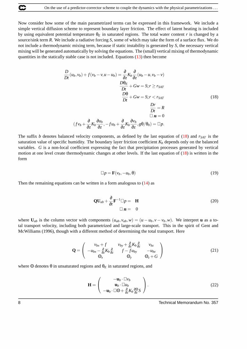
Now consider how some of the main parametrized terms can be expressed in this framework. We include asimple vertical diffusion scheme to represent boundary layer friction. The effect of latent heating is includedby using equivalent potential temperatureθE in saturated regions. The total water contentr is changed by asource/sink termR. We include a radiative forcingS, some of which may take the form of a surface flux. We donot include a thermodynamic mixing term, because if static instability is generated byS, the necessary verticalmixing will be generated automatically by solving the equations. The (small) vertical mixing of thermodynamicquantities in the statically stable case is not included. Equations (13) then become

DDt

(ub,vb)+ f (vb−v,u−ub) =∂∂z

Kb∂∂z

(ub−u,vb−v)

DθE

Dt+Gw= S; r ≥ rSAT

DθDt

+Gw= S; r < rSAT (18)

DrDt

= R

∇.u = 0

( f vb +∂∂z

Kb∂ub

∂z,− f ub +

∂∂z

Kb∂vb

∂z,gθ/θ0) = ∇p.

The suffix b denotes balanced velocity components, as defined by the last equation of (18) and rSAT is thesaturation value of specific humidity. The boundary layer friction coefficientKb depends only on the balancedvariables. G is a non-local coefficient expressing the fact that precipitation processes generated by verticalmotion at one level create thermodynamic changes at other levels. If the last equation of (18) is written in theform

∇p = F(vb,−ub,θ) (19)

Then the remaining equations can be written in a form analogous to (14) as

QUab+∂∂t

F−1∇p = H (20)

∇.u = 0

whereUab is the column vector with components(uab,vab,w) = (u− ub,v− vb,w). We interpretu as a to-tal transport velocity, including both parametrized and large-scale transport. This in the spirit of Gent andMcWilliams (1996), though with a different method of determining the total transport. Here

Q =

vbx+ f vby+ ∂∂zKb

∂∂z vbz

−ubx− ∂∂zKb

∂∂z f − f uby −ubz

Θx Θy Θz+G

(21)

whereΘ denotesθ in unsaturated regions andθE in saturated regions, and

H =

−ub ·∇vb

ub ·∇ub

−ub ·∇Θ+ ∂∂zKb

∂Θ∂z S

. (22)



Figure 2: Fluid element pictures showing a vertical cross-section of a frontal zone with moisture. Left: thehatched elements are moist. Right: the striped elements have been cooled by precipitation falling from theconvecting hatched elements.

We can then derive a generalised omega equation

∇× (FQUab) = ∇× (FH) (23)

Equation (23) shows that the unbalanced wind is a response to the forcingH which includes advection by thebalanced wind and the thermal forcing. The magnitude of the response again depends on the potential vorticitymatrix Q. We can see from (21) that the effect of friction is to increase the positive definiteness ofQ, and thusreduce the amplitude of the response to forcing. The effect of latent heating is to increase the response. IfQ has a region with zero eigenvalues, the response to forcing will take the form of dry mixing, moist mixing(shallow convection), or immediate penetrative convection according to the nature of the current state. Theoverall ageostrophic circulation includes the net transport due to the mixing or convection. An example ofthe penetrative convection case is shown in Fig. 2, generated by the code used in Shutts et al.(1988). Thedata represent a low-level frontal discontinuity. The evolution is driven by a large-scale deformation fieldwhich compresses the vertical cross-section illustrated. The hatched elements in the boundary layer are moist,and potentially unstable. In the left-hand picture, the deformation drives ascent at the front, which results inseveral elements convecting to a new equilibrium level. The right-hand picture shows the effect of including thecooling effect of the resulting precipitation, an example of the termG in (18). The descent of elements underthe convecting elements causes enhanced low-level convergence which increases the amount of convection.However, the total mass exchange is still determined by having to maintain geostrophic balance against theeffect of the large-scale convergence. This total transport is the unbalanced circulationUab that appears in (20).

Following the methods of the previous subsection, we now suppose that (20) acts as a reduced system for thefull equations including physics. A key property of this equation is that the total unbalanced circulation isuniquely determined by the large-scale forcing. In a primitive equation model, the vertical motion, boundarylayer mixing coefficients, and convective mass fluxes are all separate variables. There is thus a possibility thatthe same overall mass transport can be achieved by many different combinations of resolved and parametrizedtransports. This can be avoided if the parametrized transports are functions of ’slow’ variables only, so that thetotal transport needed to maintain large-scale balance is then made up by resolved vertical motion. However,



if the parametrized fluxes depend on the large-scale vertical motion, or the horizontal divergence, there is adanger of multiple solutions and unstable feedback loops. Some other, more detailed requirements are listedbelow:

i) The boundary layer vertical diffusion of momentum must be implemented in a way that maintains Ekmanbalance (last equation of (18)) as a limit solution. The current ECMWF implementation, Beljaars (1991)includes this.

ii) The effect of large-scale latent heating should be incorporated in a way that is consistent with the effectof vertical motion on the dry air. This is achieved at ECMWF by averaging the increments from the cloudscheme, which are largely driven by the local vertical motion, along the trajectory in the same way as theexplicit dynamics, Wedi (1999).

iii) The parametrized transports should be determined implicitly. This can be partly achieved in the predictor-corrector scheme, which is a first iteration towards a fully implicit scheme.

2.4 Implementation of a predictor-corrector algorithm using the current ECMWF parametriza-tions

We now seek to apply the principles of the previous two subsections to the current ECMWF parametrizations.Details of these parametrizations are set out in Gregory (2000) and references therein, together with ECMWFinternal documentation available on request.

All the parametrizations contain fast processes, but the final increment obtained from each parametrizationscheme should only vary on a slow time-scale, which is well-resolved by the model time-step. We use schemes(9) or (10) to integrate fast and slow processes, and use the structure of (20) to guide the separation of time-scales. The resulting scheme has to be more complex than (9) or (10) because of the presence of fast time-scalesin the resolved dynamics. Essentially the procedure has to be carried through twice, though only two evaluationsof each function are needed in each predictor-corrector time-step. The general procedure is:

i) The first and third equations of (9) or (10) are used to estimate increments from the dynamics and radiation.

ii) The second and fourth equations of (9) or (10) are then used to integrate the vertical diffusion, gravity wavedrag, cloud and (ideally) convection. However, an implicit form of the ECMWF convection scheme is notcurrently available.

iii) These increments are then combined with the resolved dynamics, using the first and third equations.

iv) The fast dynamics is accounted for by using the second and fourth equations to solve for the vertical motion.

Care is required in applying this procedure with semi-Lagrangian advection. Consider the simple equation

DuDt

= U +V (24)

whereU andV are large, so thatu is a fast variable and the reduced equation isU +V = 0. Then the naturalimplicit scheme is

ut+δta −ut

d =12

δt((U +V)t

d +(U +V)t+δta

)(25)

The form of this equation suggests that we treatµ≡ U +V as a slow variable, which we have to estimate



separately at timet and timet + δt. The overall scheme will then be second-order accurate for the reducedsystem, as required. If we assume thatU is given, but thatV depends onu, these estimates can be made bysolving

(uo−ut)a = δt(U +Vo)a (26)

(uO−ut+δt)a = uOa −ut

d = δt(U +VO)a

for uoa,u

Oa respectively, and settingµt

a = (δt)−1(uo−ut)a,µt+δta = (δt)−1(uO−ut+δt)a. The replacement ofut+δt

aby ut

d follows because all the contributions toDu/Dt are accounted for inU +V. The implicit scheme (25) isthen approximated by the predictor-corrector scheme as above. Equation (26) respects the formulation of theparametrizations, represented byV, as calculations at single columns of grid-points.

We illustrate this first with the scheme used for the vertical diffusion of theu component of the wind:

(uo−ut)a = δt

(U t +

∂∂z

Ktb

∂uo

∂z

)a

u∗a−utd =

12

δt((uo−ut)d +(uo−ut)a +other physics+Pu∗a

)(27)

uOa −ut

d = δt

(U∗+

∂∂z

K∗b∂uO

∂z

)a

ut+δta −ut

d =12

δt((uo−ut)d +(uO

a −utd)+other physics+Put+δt

a

)Here,U denotes increments from the resolved dynamics and/or other parametrized processes (calculated in step(i)), andP represents the semi-implicit part of the model (calculated in step (iv)). This scheme approximatesthe reduced equation

U +∂∂z

K∂u∂z

= 0 (28)

In this paper,U only includes increments from the resolved dynamics so that, in the formulation illustrated in(18), we would haveU =− ∂p

∂x + f v. We implement the gravity wave drag scheme in the same way, since partof that scheme represents low level drag due to unresolved hills. The equivalent term toU now includes thevertical diffusion increments, to prevent possible double-counting.

Similar equations to (27) represent the thermodynamic equation in the boundary layer. The first equation takesthe form for the dry case

θo−θt = Wt +∂∂z

Ktb

∂θo

∂z(29)

In (20), we expect that any instability generated by the source termSwill have to be compensated by verticalmixing, so that the termW needs to include radiative and surface flux terms. Since the resolved dynamics inthe ECMWF model expresses conservation ofθ along trajectories, it does not contribute toW.

The prognostic cloud scheme takes the form of evolution equations of the formDlDt = C−Dl for cloud water,l ,

and cloud amount. Here,C,D are respectively the rate of generation of cloud water and the rate of destruction



by precipitation.C is dominated by a term proportional to the vertical motion and is associated with latentheat release. We can write this as a source termLw in the thermodynamic equation, withL being the locallatent heat (water or ice). The cloud sink termDl generates a (non-local) source termV in the thermodynamicequation associated with evaporation of precipitation. The thermodynamic equation can thus be written asDθDt = L(C)w+V(Dl). The cloud liquid water and thermodynamic equations are integrated as follows:

za−zd =12

δt(wtd +wt

a)

l∗d = l tdexp(−Dtdδt)+

Ctd

Dtd(1−exp(−Dt

dδt))

Lt = L(Ct),Vt = V(Dt l t)

θ∗a−θtd =

12

δt(Lt

dwtd +Lt

awta +Vt

d +Vta +Pθ∗a

)(30)

zt+δta −zt

d =12

δt(wtd +w∗a)

lOa = l tdexp(−D∗aδt)+

C∗aD∗a

(1−exp(−D∗aδt))

θt+δta −θt

d =12

δt(

Ltdwt

d +L∗aw∗a +Vtd +V∗a +Pθt+δt

a

)where the equations for calculating the vertical coordinatezd of the departure point from the vertical velocityare included to demonstrate the overall structure, andP represents the semi-implicit correction. The reducedequation approximated by this scheme is

C = Dl (31)DθDt

= Lw+V(Dl)

Using the first of these equations and the fact thatC is largely a function ofw, the second equation can bewritten asDθE

Dt = V(w), whereV is a non-local function ofw. This is consistent with (21). The scheme (30)thus implies a second-order accurate approximation to (31) as desired.

The equations solved in the convection scheme take the form

uc−ut =1ρ

δt∂∂z

(Mup(uup−u)+Mdown(udown−u)) (32)

There are similar equations for the other model variables. The mass-fluxesMup,Mdown are complex nonlinearfunctions of the atmospheric state.u represents an environmental value ofu, while uup andudownare updraughtand downdraught values. This scheme is formulated explicitly, so has to be integrated differently from the otherparametrizations. The natural method consistent with the predictor-corrector scheme for the resolved dynamicsis

u∗−ut =12

δt

[U t +

1ρt

∂∂z

(Mt

up(utup−ut)+Mt

down(utdown−ut)

)]d+



12

δt

[U t +

1ρt

∂∂z

(Mt

up(utup−ut)+Mt

down(utdown−ut)

)]a+δtPu∗ (33)

ut+δt −ut =12

δt

[U t +

1ρt

∂∂z

(Mt

up(utup−ut)+Mt

down(utdown−ut)

)]d+

12

δt

[U∗+

1ρ∗

∂∂z

(M∗

up(u∗up−u∗)+M∗

down(u∗down−u∗)

)]a+δtPut+δt

whereU andP play the same role as in (27). This allows the explicit vertical motion to combine with theconvective environmental mass flux in achieving a total vertical transport(w+Mup+Mdown) of each variable,though there is still an inconsistency between the semi-Lagrangian treatment of the resolved dynamics and theflux form treatment of the convective transports. The use of a predictor-corrector scheme gives the opportunityfor an implicit adjustment of the convective mass flux.

We note that this formulation assumes that the mass fluxesM are slow variables, with the same time scaleas the explicit vertical motion. However,M is actually chosen to allow instability in the model profile to beremoved rapidly, and would thus be more naturally formulated as a fast process like the vertical diffusion. Thiswould require a change in the formulation of the convection scheme to allow the fast changes due to convectionto balance the other processes which create instability, giving an equation of the form (24). Such a schemewould give behaviour closer to the balanced solution illustrated in Fig. 2 and be more consistent with the otherparametrizations.

3 Examples of performance

The analysis of the previous section shows that a more accurate time integration of the combined dynamics andparametrizations can be obtained using the predictor-corrector approach. However, the overall performanceof the combined system depends also on the formulation of the parametrization schemes, and so the cost-effectiveness of the predictor-corrector scheme cannot be judged until the parametrizations have been optimisedto work within this context. The results shown in this paper are direct comparisons between the operationalextrapolated scheme of Wedi (1999) and the predictor-corrector scheme. They use a version of the model withTL511 horizontal resolution and 60 levels (Cycle 23R4) tested on a set of 14 cases distributed between August1998 and December 1999. The analyses were reruns of the operational analyses using a TL511 model. Thesecases formed the second set used by Cullen (2001). The forecasts were run with both the operational 15-minute time-step and a 20-minute time-step, to see if the improved accuracy of the predictor-corrector schemereduces the sensitivity to the time-step and, in particular, would allow a longer time-step. The cases were alsorun using a second iteration of the predictor-corrector scheme. If the predictor-corrector scheme is iterated toconvergence, the limit scheme would be a centred fully-implicit scheme. By comparing the results from oneand two iterations, we can see if convergence is occurring, and, if so, estimate the benefit that could be obtainedfrom a fully implicit scheme. Non-convergence of the iteration would suggest that there are undesirable featuresof the model formulation.

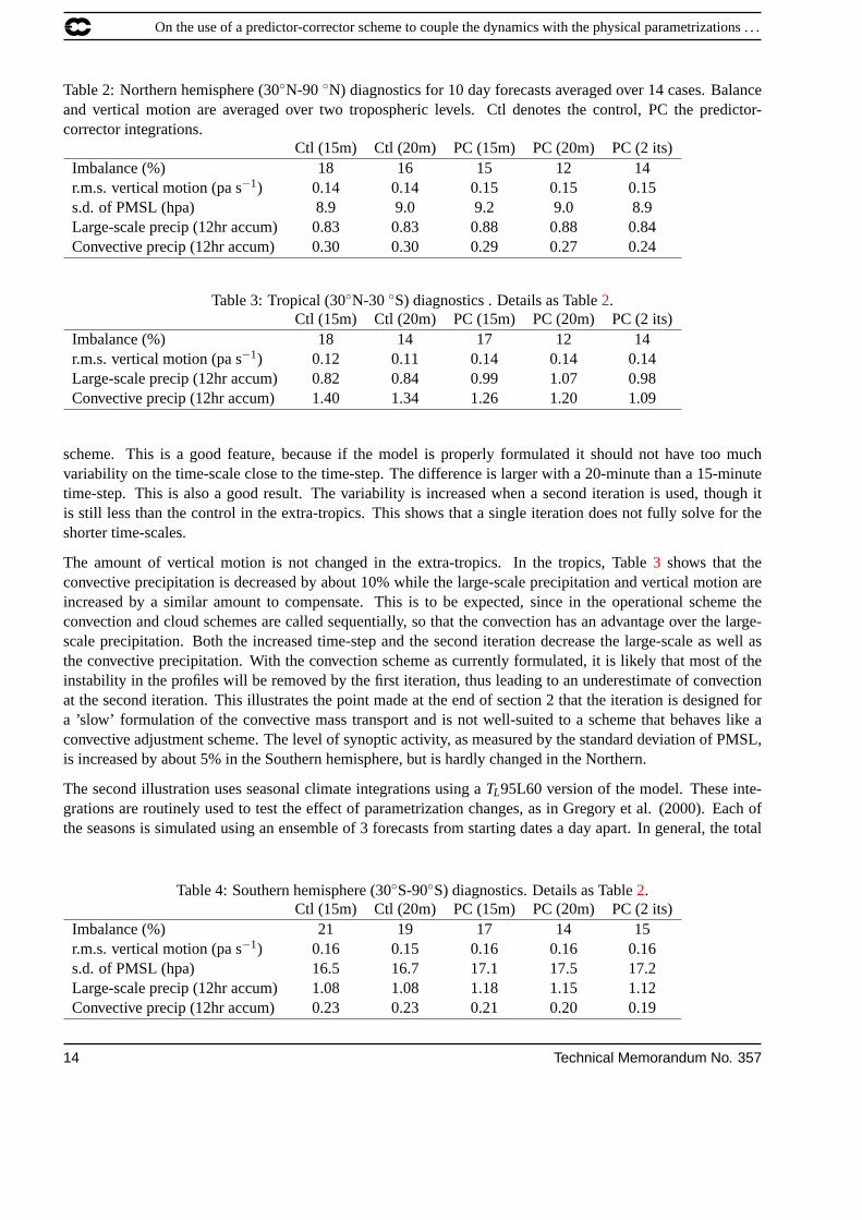
Tables2-4 shows the averaged statistics obtained over the 14 cases. The diagnostics chosen are those that areexpected to be the most sensitive to model changes. We show the effect of increasing the time-step from 15to 20 minutes in both the operational scheme and the predictor-corrector scheme; also the effect of the seconditeration of the predictor-corrector scheme with a 20 minute time-step. The ’imbalance’ statistic measures theratio of the r.m.s. second time differenceDt+δt −2Dt +Dt−δt to the r.m.s. divergence itself. It is rescaled by afactor 9/16 for the 20 minute time-step so that the two time-steps can be compared as second time derivatives.

Tables2 and4 show that the short time variability of the divergence is reduced by using the predictor-corrector



Table 2: Northern hemisphere (30◦N-90 ◦N) diagnostics for 10 day forecasts averaged over 14 cases. Balanceand vertical motion are averaged over two tropospheric levels. Ctl denotes the control, PC the predictor-corrector integrations.

Ctl (15m) Ctl (20m) PC (15m) PC (20m) PC (2 its)Imbalance (%) 18 16 15 12 14r.m.s. vertical motion (pa s−1) 0.14 0.14 0.15 0.15 0.15s.d. of PMSL (hpa) 8.9 9.0 9.2 9.0 8.9Large-scale precip (12hr accum) 0.83 0.83 0.88 0.88 0.84Convective precip (12hr accum) 0.30 0.30 0.29 0.27 0.24

Table 3: Tropical (30◦N-30 ◦S) diagnostics . Details as Table2.Ctl (15m) Ctl (20m) PC (15m) PC (20m) PC (2 its)

Imbalance (%) 18 14 17 12 14r.m.s. vertical motion (pa s−1) 0.12 0.11 0.14 0.14 0.14Large-scale precip (12hr accum) 0.82 0.84 0.99 1.07 0.98Convective precip (12hr accum) 1.40 1.34 1.26 1.20 1.09

scheme. This is a good feature, because if the model is properly formulated it should not have too muchvariability on the time-scale close to the time-step. The difference is larger with a 20-minute than a 15-minutetime-step. This is also a good result. The variability is increased when a second iteration is used, though itis still less than the control in the extra-tropics. This shows that a single iteration does not fully solve for theshorter time-scales.

The amount of vertical motion is not changed in the extra-tropics. In the tropics, Table3 shows that theconvective precipitation is decreased by about 10% while the large-scale precipitation and vertical motion areincreased by a similar amount to compensate. This is to be expected, since in the operational scheme theconvection and cloud schemes are called sequentially, so that the convection has an advantage over the large-scale precipitation. Both the increased time-step and the second iteration decrease the large-scale as well asthe convective precipitation. With the convection scheme as currently formulated, it is likely that most of theinstability in the profiles will be removed by the first iteration, thus leading to an underestimate of convectionat the second iteration. This illustrates the point made at the end of section 2 that the iteration is designed fora ’slow’ formulation of the convective mass transport and is not well-suited to a scheme that behaves like aconvective adjustment scheme. The level of synoptic activity, as measured by the standard deviation of PMSL,is increased by about 5% in the Southern hemisphere, but is hardly changed in the Northern.

The second illustration uses seasonal climate integrations using aTL95L60 version of the model. These inte-grations are routinely used to test the effect of parametrization changes, as in Gregory et al. (2000). Each ofthe seasons is simulated using an ensemble of 3 forecasts from starting dates a day apart. In general, the total

Table 4: Southern hemisphere (30◦S-90◦S) diagnostics. Details as Table2.Ctl (15m) Ctl (20m) PC (15m) PC (20m) PC (2 its)

Imbalance (%) 21 19 17 14 15r.m.s. vertical motion (pa s−1) 0.16 0.15 0.16 0.16 0.16s.d. of PMSL (hpa) 16.5 16.7 17.1 17.5 17.2Large-scale precip (12hr accum) 1.08 1.08 1.18 1.15 1.12Convective precip (12hr accum) 0.23 0.23 0.21 0.20 0.19



precipitation is increased by about 1%, but the convective precipitation is reduced by almost 10%, consistentwith the high resolution results shown above. The results for the Northern hemisphere winter are shown inFig.3. The ITCZ is shifted southwards over the East Pacific and the total rainfall is increased over the Atlanticand near the dateline. Southern Africa and an area to the east of Australia are drier. The western parts of thesub-tropical oceans in the southern hemisphere are wetter. The Northern hemisphere storm-tracks are displacedsouthwards. In the Northern hemisphere summer (not shown), the ITCZ is again more intense near the dateline.It is displaced southwards over the Atlantic abut northwards north of Australia. Western Europe and centraland eastern North America are wetter. The southern hemisphere storm-track is displaced northward in theAustralian sector. Verification against GPCP data (not shown) indicates that the differences form a significantfraction of the difference between model and climatology in a number of places, showing that the effects aresignificant. However, the level of agreement between model and climatology is not very different between thetwo sets of integrations.

The third illustration shows the convective rainfall prediction for an area in the tropics. We compare the oper-ational scheme with the predictor-corrector scheme and the predictor-corrector scheme with a second iteration.All integrations use a 20 minute time-step. The results shown in Fig. 4 are a 24 hour accumulation betweenT+12 and T+36 of a forecast starting from 10 August 1999. The overall patterns are similar, since sufficienttime has not elapsed to allow the large-scale patterns to diverge. The predictor-corrector scheme gives smootherfields in regions where the total convective amounts are small. This is consistent with the exclusion of the re-solved dynamics from the termW in equation (29). The second iteration reduces the amount of convectionsubstantially, especially over the ocean in the eastern half of the area shown. The reason is again the way theconvection is formulated, as discussed at the end of section 2.

We finally illustrate the effect of the scheme on Northern hemisphere performance using scatter plots of theanomaly correlation of 7-day forecasts of the 500hpa geopotential. The choice of day 7 is to allow the changesto the model to become clear, as short-range forecast errors are usually dominated by the analysis. However,there is still substantial deterministic skill at this time range. The results are shown in Fig. 5. The change fromthe operational scheme to the predictor-corrector scheme produces on average a positive impact. The spreadis quite large, so that the difference is only statistically significant at the 5% level. Results from other time-ranges (not shown) show that the predictor-corrector scheme is worse at day 3, but that statistically significantimprovements are also obtained at 1000hpa at day 5. A proper assessment of the effect on 3-day forecastscannot be made without performing a data assimilation experiment.

The effect of changing the time-step is much smaller than the change of scheme if measured in terms of spreadof impacts. This is true whether the operational or the predictor-corrector scheme is used. The operationalscheme is slightly more sensitive to the change in time-step, as indicated by the significance test. Results fromother time ranges show that the increased time-step gives significantly worse results at day 3 in both the controland predictor-corrector experiments. In the control experiment, there are significant improvements as well asdeteriorations at later times. In the predictor-corrector experiment there are no further significant impacts tillday 9.

The second iteration has a larger effect than changing the time-step, though not as large as the replacement ofthe operational scheme by the predictor-corrector scheme. The effect is consistently good at day 3 (not shown),removing the deterioration of the predictor-corrector against the control at this time mentioned above. At day 7,the effect is not consistently good or bad and so does not suggest that a fully converged scheme would performbetter than a single iteration.



60°S�

60°S

30°S 30°S�

0°�

0°

30°N 30°N�

60°N�

60°N

135°W�

135°W 90°W

90°W 45°W

45°W 0°

0° 45°E

45°E 90°E

90°E 135°E�

135°E

0.2�

1

2�

3�

5�

8�

16

32�

60°S

60°S

30°S 30°S

0°�

0°

30°N 30°N

60°N

60°N

135°W�

135°W 90°W

90°W 45°W

45°W 0°

0° 45°E

45°E 90°E

90°E 135°E�

135°E

-16

-8

-2

-0.5

0.5�

2�

8�

16

60°S�

60°S

30°S 30°S�

0°�

0°

30°N 30°N�

60°N�

60°N

135°W�

135°W 90°W

90°W 45°W

45°W 0°

0° 45°E

45°E 90°E

90°E 135°E�

135°E

-16

-8

-2

-0.5

0.5

2�

8�

16

Figure 3: 3-month mean precipitation for Northern hemisphere winter. Forecasts used mean of 3 simulations foreach season. Top: predictor-corrector, middle: difference predictor-corrector minus control, bottom: differencein convective precipitation predictor-corrector minus control. Units are mm/day. Contours as shown on eachpanel.



Figure 4: 24 hour accumulation between T+12 and T+36 of convective precipitation for forecasts startingfrom 10 August 1999. Contours at 1,2,4,8,16,32,64mm. Top: control, middle: predictor-corrector, bottom:predictor-corrector with 2 iterations.



168 HOUR FORECASTS

AREA=N.HEM TIME=12 DATE=19980825/...

ANOMALY CORRELATION FORECAST

500 hPa GEOPOTENTIAL (%)

100 90 80 70 60 50 40 30 20 10

Impphys100

90

80

70

60

50

40

30

20

10

CT

L

Impphys is BETTER than CTL at the 5.0% level (t test)Impphys is BETTER than CTL at the 10.0% level (sign test)

14 CASES

MEAN

MAGICS 6.3 styx - nac Fri Dec 7 14:43:31 2001 Verify SCOCAT

168 HOUR FORECASTS




100 90 80 70 60 50 40 30 20 10

control 20m100

90

80

70

60

50

40

30

20

10

con

tro

lcontrol 20m is WORSE than control at the 10.0% level (t test)

14 CASES

MEAN

MAGICS 6.3 styx - nac Thu Oct 11 15:44:59 2001 Verify SCOCAT

168 HOUR FORECASTS




100 90 80 70 60 50 40 30 20 10

Impphys 20m100

90

80

70

60

50

40

30

20

10

Imp

ph

ys

14 CASES

MEAN

MAGICS 6.3 styx - nac Thu Dec 27 11:19:03 2001 Verify SCOCAT

168 HOUR FORECASTS




100 90 80 70 60 50 40 30 20 10

Impphys 2 its100

90

80

70

60

50

40

30

20

10

Imp

ph

ys

14 CASES

MEAN

MAGICS 6.3 styx - nac Thu Dec 27 11:11:59 2001 Verify SCOCAT

Figure 5: Scatter plots of anomaly correlations (percent) of 500hpa height over the Northern hemisphere for 14test cases. Top left: Predictor-corrector scheme plotted against the control (15 minute time-step).Top right: 20minute time-step control plotted against 15 minute time-step control. Bottom left: 20 minute predictor-correctorplotted against 15 minute predictor-corrector. Bottom right: Predictor-corrector with 2 iterations plotted againstsingle iteration (15 minute time-step).



4 Discussion

We have shown that the predictor-corrector scheme is competitive in accuracy for given cost for a simpleproblem with multiple time-scales. We have also shown that, because parametrized processes form an integralpart of the equations describing large-scale balance, it is desirable to determine the parametrized transportsimplicitly, along with the resolved transports. The predictor-corrector scheme provides a framework for doingthis which may give it an advantage over single-step schemes with a shorter time-step.

We illustrate an implementation using current ECMWF parametrization schemes. It is clear that the replace-ment of the operational scheme by the predictor-corrector scheme has a significant impact on large-scale perfor-mance, which demonstrates that the integration of resolved and parametrized inputs to a model is an importantarea to get right. In general, large-scale scores in the Northern hemisphere are improved and others are neutral.The short-time variability is reduced. The results with a second iteration show that the results from a singleiteration are still some way from those that would be obtained by a fully implicit scheme. A major factor inthis is that the convection scheme is not well-suited to this framework. A different formulation of convectionis required if this sort of integration scheme is to perform at its best. More generally, better performance of aniterative scheme needs parametrizations which vary smoothly with input data, as already found desirable fordata assimilation applications.

Acknowledgements

The authors wish to thank many colleagues at ECMWF, particularly Christian Jakob, with help and explana-tions of the parametrization code and supply of diagnostic programmes. The integrations shown in Fig.2 wereperformed by M.W.Holt.

References

Beljaars,A.C.M. (1991): Numerical schemes for parametrizations;Proc. ECMWF seminar on ’Numericalmethods in atmospheric models, 308-334.

Browning,G. and Kreiss,H-O. (1994): Splitting methods for problems with different time-scales;Mon. WeatherRev., 122, 2614-2622.

Cullen,M.J.P. (2001): Alternative implementations of the semi-Lagrangian semi-implicit scheme in the ECMWFmodel;Quart. J. Roy. Meteorol. Soc., 127, 2787-2802.

Cullen,M.J.P., Norbury,J., Purser,R.J. and Shutts,G.J. (1987): Modelling the quasi-equilibrium dynamics of theatmosphere;Quart. J. Roy. Meteorol. Soc., 113, 735-758.

Gent,P.R. and McWilliams,J.C. (1996): Eliassen-Palm fluxes and the momentum equation in non-eddy-resolvingocean circulation models;J.Phys. Oceanog., 26, 2539-2546.

Gregory,D., Morcrette,J.-J., Jakob,C., Beljaars,A.,C.,M. and Stockdale,T. (2000): Revision of convection, ra-diation and cloud schemes in the ECMWF Integrated Forecasting System;Quart. J. Roy. Meteorol. Soc., 126,1685-1710.

Hoskins,B.J. (1975): The geostrophic momentum approximation and the semi-geostrophic equations;J. Atmos.Sci., 32, 233-242.



MacDonald,A. and Haugen,J. (1992): A two-time-level, three dimensional, semi-Lagrangian, semi-implicit,limited area, grid-point model of the primitive equations;Mon. Weather Rev., 120, 2603-2621.

MacDonald,A. (1998): The origin of noise in semi-Lagrangian integrations;Proc. ECMWF seminar on ’Recentdevelopments in numerical methods for atmospheric modelling, 308-334.

Mahfouf,J.-F. and Rabier,F. (2000): The ECMWF operational implementation of four-dimensional variationaldata assimilation. II: Experimental results with improved physics;Quart. J. Roy. Meteorol. Soc., 126, 1171-1190.

Moorthi,S., Higgins,R.W. and Bates,J.R. (1995): A global multilevel atmospheric model using a vector semi-Lagrangian finite-difference scheme. Part II: version with physics;Mon. Weather Rev., 123, 1523-1541.

Schubert,W.H. (1985): Semi-geostrophic theory;J. Atmos. Sci., 42, 1770-1772.

Shutts,G.J., Cullen,M.J.P. and Chynoweth,S. (1988): Geometric models of balanced semi-geostrophic flow;Ann. Geophysicae, 6(5),493-500.

Sportisse, B. (2000): An analysis of operator splitting techniques in the stiff case;J. Comput. Phys., 161,140-168.

Temperton,C., Hortal,M. and Simmons,A.J. (2001): A two-time-level semi-Lagrangian global spectral model;Quart. J. Roy. Meteorol. Soc., 127, 111-128.

Wedi,N.P. (1999): The numerical coupling of the physical parametrizations to the ”dynamical” equations in aforecast model;ECMWF Tech. Memo., no. 274..


Documents

Use Predictor Corrector Scheme - ECMWF